THE CLASSICAL VERSION OFSTOKES’ THEOREM REVISITED

STEEN MARKVORSEN#

Abstract. Using only fairly simple and elementary considera-tions - essentially from first year undergraduate mathematics - weshow how the classical Stokes’ theorem for any given surface andvector field in R3 follows from an application of Gauss’ divergencetheorem to a suitable modification of the vector field in a tubularshell around the given surface. The two stated classical theoremsare (like the fundamental theorem of calculus) nothing but shad-ows of the general version of Stokes’ theorem for differential formson manifolds. The main points in the present paper, however, isfirstly that this latter fact usually does not get within reach forstudents in first year calculus courses and secondly that calculustextbooks in general only just hint at the correspondence alludedto above. Our proof that Stokes’ theorem follows from Gauss’ di-vergence theorem goes via a well known and often used exercise,which simply relates the concepts of divergence and curl on thelocal differential level. The rest of the paper uses only integrationin 1, 2, and 3 variables together with a ’fattening’ technique forsurfaces and the inverse function theorem.

1. Introduction

One of the most elegant and useful results concerning vector fieldsin R3, is the classical version of Stokes’ theorem. It is one of thoseimportant results, which is so nicely molded from analysis, calculus,geometry, and linear algebra that it forms a solid basis for and indeedan integral part of the final fireworks and climax of first year under-graduate mathematics education. At the same time Stokes’ theorempoints forward into a wealth of deep applications in electromagnetism,in fluid dynamics, and in mathematics itself, to mention but a few ofthe most significant fields of applications. Such results serve as indis-pensable bootstraps for university students en masse - be they studentsof engineering, of physics, of biology, of chemistry, of mathematics, etc.;see e.g. [FLS], [She].

2000 Mathematics Subject Classification. Primary 26.Key words and phrases. Stokes’ theorem, Gauss’ divergence theorem, level sur-

faces, gradient flow, shells, undergraduate mathematics, didactics, visualization.#The author would like to thank the Learning Lab DTU for kind hospitality, for

rewarding discussions on didactics, and for technical and financial support.1

2 S. MARKVORSEN

It is the purpose of this paper to facilitate the presentation, i.e.the undergraduate teaching, of Stokes’ theorem by suggesting and un-folding a proof, which shows that it is a direct consequence of Gauss’divergence theorem. In the process there are also a few other useful in-sights and geometric observations to be (re)visited. The first pertinentobservation is the following quotation from [C] concerning the historyof Stokes’ theorem (see also [K] p. 790):

The history of Stokes’ Theorem is clear but very com-plicated. It was first given by Stokes without proof -as was necessary - since it was given as an examina-tion question for the Smith’s Prize Examination of thatyear [1854]! Among the candidates for the prize wasMaxwell, who later traced to Stokes the origin of thetheorem, which by 1870 was frequently used. On thissee George Gabriel Stokes, Mathematical and PhysicalPapers, vol. V (Cambridge, England, 1905), 320–321.See also the important historical footnote which indi-cates that Kelvin in a letter of 1850 was the first whoactually stated the theorem, although others as Amperehad employed ”the same kind of analysis ... in particularcases.”

M. J. Crowe, [C] p. 147.

Gauss’ divergence theorem is of the same calibre as Stokes’ theorem.They are both members of a family of results which are concerned with’pushing the integration to the boundary’. The eldest member of thisfamily is the following:

Theorem 1.1 (Fundamental theorem of calculus). Let f be a conti-nuous function on R. Then the function

A(x) =

∫ x

0

f(u) du

is differentiable with

(1.1) A′(x) = f(x) ,

and moreover, if F (x) is any (other) function satisfying F ′(x) = f(x),then

(1.2)

∫ b

a

f(u) du = F (b)− F (a) .

The message of this theorem is that two fundamental problems - thatof finding a function whose derivative is a given function and that offinding the average of a given function - have a common solution. It isalso the first result which displays - in equation (1.2) - the astoundingsuccess of ’pushing the integration to the boundary’. Compare with

STOKES’ THEOREM 3

the main ’actors’ of the present paper, Theorems 1.3 and 1.4 below.

The divergence theorem is not - conceptually speaking - ’far’ fromthe fundamental theorem of calculus. Most textbook proofs of thedivergence theorem covers only the special setting of a domain whoseboundary consists of the graphs of two functions, each of two variables.This enables in fact a direct proof in this special case via Theorem 1.1,see [EP] pp. 1058–1059. Stokes’ theorem is a little harder to grasp,even locally, but follows also in the corresponding setting (for graphsurfaces) from Gauss’ theorem for planar domains, see [EP] pp. 1065–1066.

This approach suggests indirectly that the full classical Stokes’ theo-rem (for general surfaces) should follow directly from Gauss’ divergencetheorem (for general domains). The main part of the present paper willbe devoted to a proof following this idea.

The most compact as well as the most general form of Stokes’ theo-rem reads as follows (see e.g. [Mu] p. 353, [G], [doC] pp. 60 ff., [Spi]p. 124):

Theorem 1.2 (Stokes’ theorem, general version). Let ω denote a dif-ferential (k − 1)−form on a compact orientable manifold Ωk. Supposethat Ω has a smooth and compact boundary ∂Ω with the induced orien-tation, and let dω denote the differential of ω. Then

(1.3)

∫

Ω

dω =

∫

∂Ω

ω .

This statement contains as corollaries both Gauss’ divergence theo-rem for domains in R3, and Stokes’ theorem for surfaces in R3. See e.g.[Mu] pp. 319–320. As mentioned above it is these latter theorems - notthe general version of Stokes’ theorem - that will be the main concernin this paper. Here are the statements:

Theorem 1.3 (Gauss’ divergence theorem). Let Ω denote a compactdomain in R3 with piecewise smooth boundary ∂Ω and outward pointingunit normal vector field n∂Ω on ∂Ω. Let V be a vector field in R3.Then

(1.4)

∫

Ω

div(V) dµ =

∫

∂Ω

V · n∂Ω dν .

Theorem 1.4 (Stokes’ theorem, classical version). Let F denote acompact, orientable, regular and smooth surface with piecewise smoothboundary ∂F and unit normal vector field nF . Let V be a vector fieldin R3. Then

(1.5)

∫

F

curl(V) · nF dµ =

∫

∂F

V · e∂F dσ .

4 S. MARKVORSEN

When calculating the right hand side, i.e. the tangential curve integral(the circulation of V) along the boundary ∂F , the orientation e∂F ofthe boundary must be chosen so that the cross product e∂F × nF at theboundary points away from the surface.

Outline of paper . In section 2 we recall the connection between curland divergence which was alluded to in the abstract. In the followingsections we then set up the notation and the results needed in orderto make this presentation reasonably self contained on the level of firstyear undergraduate mathematics. The main goal is to relate integrationover the shell extension of a given surface with the integration alongthe boundary surfaces of this extension. The proof of Stokes’ theoremis finally completed in section 8.

2. A bridge between divergence and curl

We begin by stating a connection between divergence and curl.

Observation 2.1 (Exercise). Let V(x, y, z) and W(x, y, z) denotetwo smooth vector fields in R3. Then the following identity holds true:

(2.1) div(V ×W) = curl(V) ·W + V · curl(W) .

In particular, if W is a gradient field for some smooth function ψ(x, y, z)in R3, i.e. W = grad(ψ) , we get from curl(grad(ψ)) = 0 :

(2.2) div(V × grad(ψ)) = curl(V) · grad(ψ) .

Using Gauss’ divergence theorem we ’lift’ this connection to the in-tegral level as follows:

Theorem 2.2. Let ψ(x, y, z) denote a smooth function in R3 and letV(x, y, z) be a vector field. Let Ω denote a compact domain in R3

with piecewise smooth boundary ∂Ω and outward pointing unit normalvector field n∂Ω on ∂Ω. Then we have the following

(2.3)

∫

Ω

div(V × grad(ψ)) dµ =

∫

∂Ω

(V × grad(ψ)) · n∂Ω dν .

Using equation (2.2) we therefore also have

(2.4)

∫

Ω

curl(V) · grad(ψ) dµ =

∫

∂Ω

(n∂Ω ×V) · grad(ψ) dν ,

In particular we get the total rotation vector (the so-called total’vorticity vector’ of fluid dynamics) of the vector field V in Ω :

Corollary 2.3.∫

Ω

curl(V) dµ =

∫

∂Ω

n∂Ω ×V dν .

STOKES’ THEOREM 5

Proof. This follows directly from equation (2.4) by choosing, in turn,ψ(x, y, z) = x, ψ(x, y, z) = y, and ψ(x, y, z) = z, so that grad(ψ)is successively one of the respective constant vectors (1, 0, 0), (0, 1, 0),and (0, 0, 1).

¤

3. The surface, the boundary, and the normal field

We parametrize a given surface F by a smooth regular map r froma compact domain D (with boundary ∂D) in the (u, v)−plane into R3:

F : r(u, v) = (x(u, v), y(u, v), z(u, v)) ∈ R3 , (u, v) ∈ D ⊂ R2 ,

where x(u, v), y(u, v), and z(u, v) are smooth functions of the parame-ters u and v.

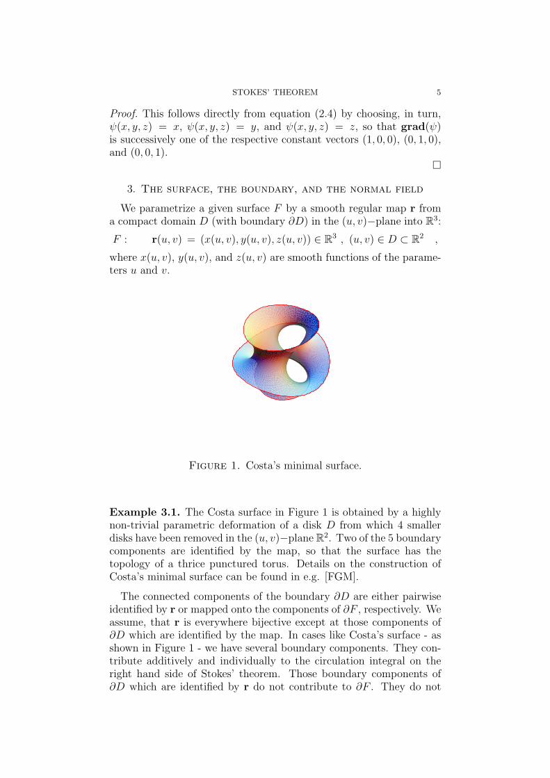
Figure 1. Costa’s minimal surface.

Example 3.1. The Costa surface in Figure 1 is obtained by a highlynon-trivial parametric deformation of a disk D from which 4 smallerdisks have been removed in the (u, v)−plane R2. Two of the 5 boundarycomponents are identified by the map, so that the surface has thetopology of a thrice punctured torus. Details on the construction ofCosta’s minimal surface can be found in e.g. [FGM].

The connected components of the boundary ∂D are either pairwiseidentified by r or mapped onto the components of ∂F , respectively. Weassume, that r is everywhere bijective except at those components of∂D which are identified by the map. In cases like Costa’s surface - asshown in Figure 1 - we have several boundary components. They con-tribute additively and individually to the circulation integral on theright hand side of Stokes’ theorem. Those boundary components of∂D which are identified by r do not contribute to ∂F . They do not

6 S. MARKVORSEN

contribute to the Stokes circulation integral either because the relevantintegrals cancel each other away. For ease of presentation and withoutlack of generality we therefore assume, that D is simply connected withonly one connected boundary component ∂D which is mapped onto ∂Fvia the map r.

A given single boundary component ∂D is parametrized as followsin the (u, v)−plane:

∂D : d(θ) = (u(θ), v(θ)) ∈ ∂D ⊂ R2 , θ ∈ I ⊂ R ,

where u(θ) and v(θ) are piecewise smooth functions of θ. The boundaryof F is then

∂F : b(θ) = r(d(θ)) = r(u(θ), v(θ)) ∈ R3 .

The Jacobians of the maps r and b are, respectively:

(3.1) Jacobir(u, v) = ‖r′u × r′v‖ , and

(3.2) Jacobib(θ) = ‖b′θ‖ .

The regularity of r is expressed by

Jacobir(u, v) > 0 for all (u, v) ∈ D .

This implies in particular, that there is a well defined unit normalvector nF = n(u, v) at each point of F :

(3.3) n(u, v) =r′u × r′v‖r′u × r′v‖

for all (u, v) ∈ D .

4. The shell fattening and a nice gradient

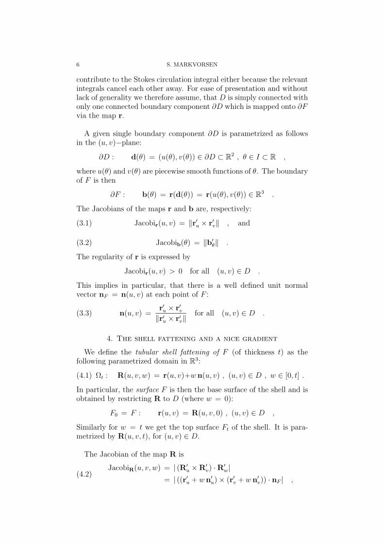
We define the tubular shell fattening of F (of thickness t) as thefollowing parametrized domain in R3:

(4.1) Ωt : R(u, v, w) = r(u, v)+w n(u, v) , (u, v) ∈ D , w ∈ [0, t] .

In particular, the surface F is then the base surface of the shell and isobtained by restricting R to D (where w = 0):

F0 = F : r(u, v) = R(u, v, 0) , (u, v) ∈ D ,

Similarly for w = t we get the top surface Ft of the shell. It is para-metrized by R(u, v, t), for (u, v) ∈ D.

The Jacobian of the map R is

(4.2)JacobiR(u, v, w) = | (R′

u ×R′v) ·R′

w|= | ((r′u + w n′u)× (r′v + w n′v)) · nF | ,

STOKES’ THEOREM 7

x y

z

x y

z

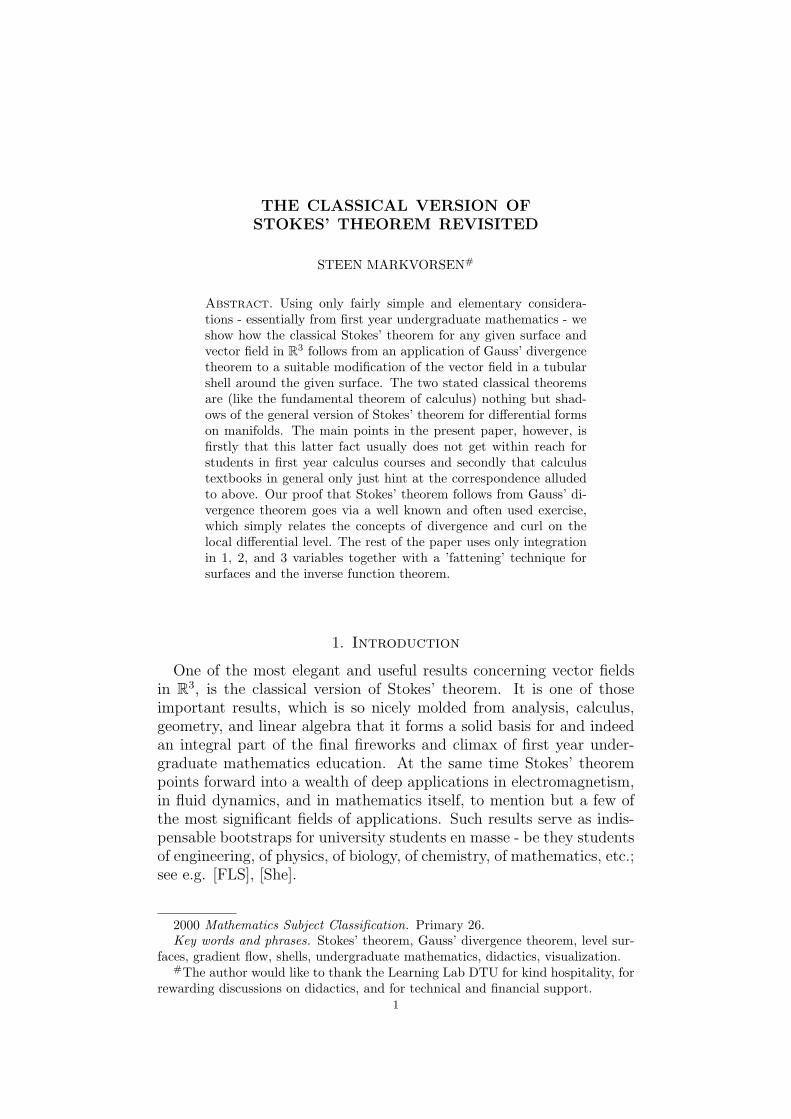
Figure 2. Two shell fattenings.

so that, since nF is a unit vector field parallel to r′u × r′v along F , weget in particular (for w = 0):

(4.3)

JacobiR(u, v, 0) = | (r′u × r′v) · nF |= ‖r′u × r′v‖= Jacobir(u, v) > 0 .

The map R is regular and bijective on D × [0, t] - provided t is suf-ficiently small. Indeed, since JacobiR(u, v, 0) > 0, this claim followsfrom the continuity of JacobiR(u, v, w) and the compactness of D.

The value of w considered as a function in Ωt ⊂ R3 is a smoothfunction of the coordinates (x, y, z) . However intuitively reasonablethis claim may seem, the precise argument goes via the inverse functiontheorem, which we state here for completeness - in its global form,without proof:

Theorem 4.1. Let Q denote an open set in Rn and let f : Q → Rn de-note a smooth bijective map with Jacobif (x) > 0 for all x ∈ Q. Thenthe inverse map f−1 : f(Q) → Q is also smooth with Jacobif−1(y) > 0for all y ∈ f(Q).

Hence, when t is sufficiently small, w is a smooth function of (x, y, z);let us call it h(x, y, z), (x, y, z) ∈ Ωt. This function then has a non-vanishing gradient, grad(h)(x, y, z), which is orthogonal to the levelsurfaces of h. In particular, grad(h) is orthogonal to the top surfaceFt of the shell Ωt, where h = t and it is orthogonal to the base surfaceF0 = F , where h = 0.

In fact, at the base surface, the field grad(h) is precisely equal tothe unit normal vector field nF . To see this we only need to show thatit has unit length: Let (u0, v0) denote a given point in D and considerthe restriction of h to the straight line r(u0, v0) + w n(u0, v0), wherew ∈ [0, t]. Let us denote r0 = r(u0, v0) and n0 = n(u0, v0). The chain

8 S. MARKVORSEN

rule then gives

(4.4)

1 = | d

dwh(r0 + w n0) |

= |n0 · grad(h)(r0 + w n0) |= ‖grad(h)(r0 + w n0) ‖ ,

so that, at the surface F , for w = 0, we have ‖grad(h)(r0)‖ = 1 andtherefore in total, as claimed above:

(4.5) grad(h)|F = nF ,

Remark 4.2. The function h(x, y, z) is in fact the Euclidean distancefrom the point (x, y, z) in Ωt to the surface F .

5. Integration in the shell

For any given smooth function f(x, y, z) defined in Ωt the integral off over that domain is:

(5.1)

∫

Ωt

f dµ

=

∫ t

0

(∫

D

f(R(u, v, w)) JacobiR(u, v, w) du dv

)dw .

The derivative of this integral with respect to the thickness t of theshell Ωt is, at t = 0, the surface integral over F :

Lemma 5.1.

(5.2)

(d

dt

)

|t=0

∫

Ωt

f dµ =

∫

F

f dν .

Proof. This follows directly from the fundamental theorem of calculus,Theorem 1.1, equation (1.1):

(5.3)

(d

dt

)

|t=0

∫

Ωt

f dµ

=

(d

dt

)

|t=0

∫ t

0

(∫

D

f(R(u, v, w)) JacobiR(u, v, w) du dv

)dw

=

∫

D

f(R(u, v, 0)) JacobiR(u, v, 0) du dv

=

∫

D

f(r(u, v)) Jacobir(u, v) du dv

=

∫

F

f dν .

¤

STOKES’ THEOREM 9

6. The wall

The shell Ωt has a boundary ∂Ωt which consists of the top levelsurface Ft, the base level surface F = F0 and a ’cylindrical wall’ surfaceWt of height t. See Figure 2. This latter component of the boundaryis simply obtained by restricting the map R to ∂D × [0, t] as follows:

Wt : B(θ, w) = R(u(θ), v(θ), w)

= r(u(θ), v(θ)) + w n(u(θ), v(θ))

= b(θ) + w n(d(θ)) , θ ∈ I , w ∈ [0, t] .

The Jacobian of this map is thus

(6.1)JacobiB(θ, w) = ‖B′

θ ×B′w‖

= ‖(b′θ + w (n d)′θ)× nF‖ ,

so that, since nF is a unit normal to the surface F and hence also tothe boundary ∂F (parametrized by b), we get in particular:

(6.2) JacobiB(θ, 0) = ‖b′θ × nF‖ = ‖b′θ‖ = Jacobib(θ) .

7. Integration along the wall

For any given smooth function g(x, y, z) defined on Wt the integralof g over that surface is

(7.1)

∫

Wt

g dν =

∫ t

0

(∫

I

g(B(θ, w)) JacobiB(θ, w) dθ

)dw .

The derivative of this integral with respect to the height t of the wallWt is, at t = 0, the line integral over ∂F :

Lemma 7.1.

(7.2)

(d

dt

)

|t=0

∫

Wt

g dν =

∫

∂F

g dσ .

Proof. This follows again from the fundamental theorem of calculus,Theorem 1.1, equation (1.1):

(7.3)

(d

dt

)

|t=0

∫

Wt

g dν

=

(d

dt

)

|t=0

∫ t

0

(∫

I

g(B(θ, w)) JacobiB(θ, w) dθ

)dw

=

∫

I

g(B(θ, 0)) JacobiB(θ, 0) dθ

=

∫

I

g(b(θ)) Jacobib(θ) dθ

=

∫

∂F

g dσ .

¤

10 S. MARKVORSEN

x

yz

x

yz

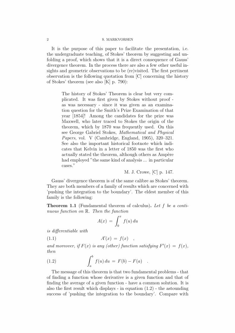
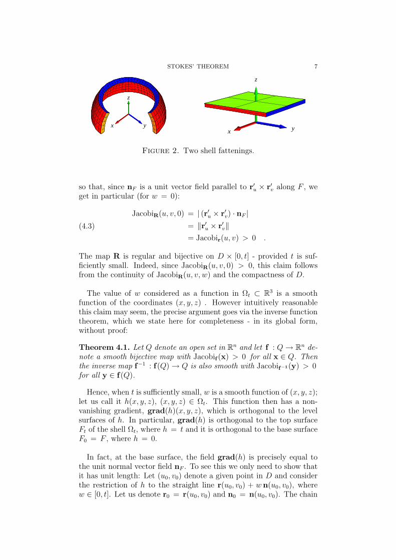
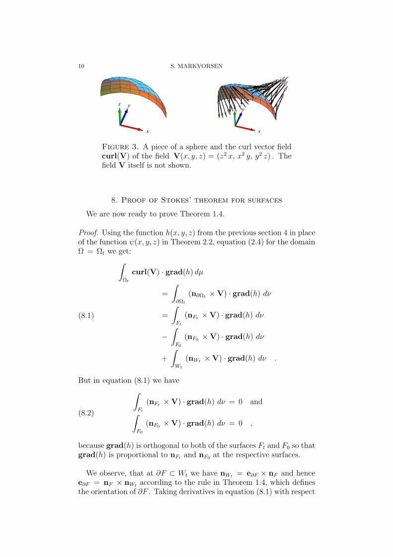
Figure 3. A piece of a sphere and the curl vector fieldcurl(V) of the field V(x, y, z) = (z2 x, x2 y, y2 z) . Thefield V itself is not shown.

8. Proof of Stokes’ theorem for surfaces

We are now ready to prove Theorem 1.4.

Proof. Using the function h(x, y, z) from the previous section 4 in placeof the function ψ(x, y, z) in Theorem 2.2, equation (2.4) for the domainΩ = Ωt we get:

(8.1)

∫

Ωt

curl(V) · grad(h) dµ

=

∫

∂Ωt

(n∂Ωt ×V) · grad(h) dν

=

∫

Ft

(nFt ×V) · grad(h) dν

−∫

F0

(nF0 ×V) · grad(h) dν

+

∫

Wt

(nWt ×V) · grad(h) dν .

But in equation (8.1) we have

(8.2)

∫

Ft

(nFt ×V) · grad(h) dν = 0 and

∫

F0

(nF0 ×V) · grad(h) dν = 0 ,

because grad(h) is orthogonal to both of the surfaces Ft and F0 so thatgrad(h) is proportional to nFt and nF0 at the respective surfaces.

We observe, that at ∂F ⊂ Wt we have nWt = e∂F × nF and hencee∂F = nF × nWt according to the rule in Theorem 1.4, which definesthe orientation of ∂F . Taking derivatives in equation (8.1) with respect

STOKES’ THEOREM 11

y

x

z

yx

z

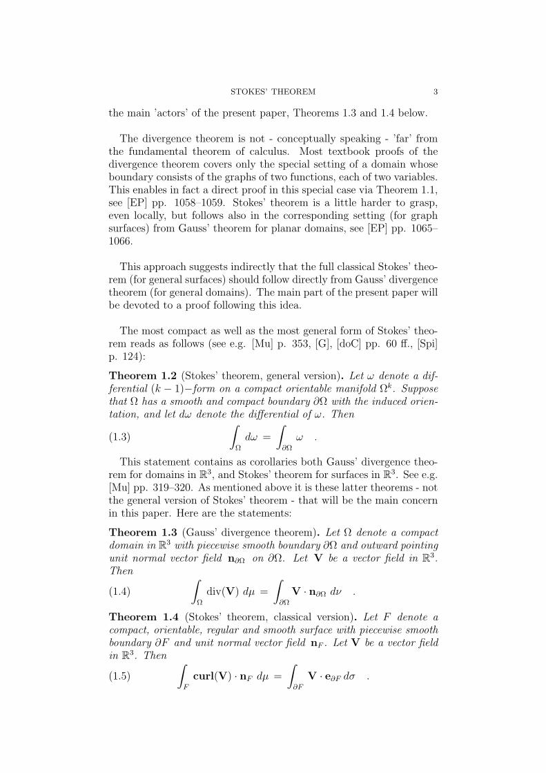
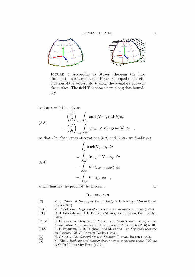
Figure 4. According to Stokes’ theorem the fluxthrough the surface shown in Figure 3 is equal to the cir-culation of the vector field V along the boundary curve ofthe surface. The field V is shown here along that bound-ary.

to t at t = 0 then gives:

(8.3)

(d

dt

)

|t=0

∫

Ωt

curl(V) · grad(h) dµ

=

(d

dt

)

|t=0

∫

Wt

(nWt ×V) · grad(h) dν ,

so that - by the virtues of equations (5.2) and (7.2) - we finally get

(8.4)

∫

F

curl(V) · nF dν

=

∫

∂F

(nWt ×V) · nF dσ

=

∫

∂F

V · (nF × nWt) dσ

=

∫

∂F

V · e∂F dσ ,

which finishes the proof of the theorem. ¤

References

[C] M. J. Crowe, A History of Vector Analysis, University of Notre DamePress (1967).

[doC] M. P. doCarmo, Differential Forms and Applications, Springer (1994).[EP] C. H. Edwards and D. E. Penney, Calculus, Sixth Edition, Prentice Hall

(2002).[FGM] H. Ferguson, A. Gray, and S. Markvorsen, Costa’s minimal surface via

Mathematica, Mathematica in Education and Research, 5 (1996) 5–10.[FLS] R. P. Feynman, R. B. Leighton, and M. Sands, The Feynman Lectures

on Physics, Vol. II, Addison Wesley (1965).[G] H. Grunsky, The General Stokes’ Theorem, Pitman, Boston (1983).[K] M. Kline, Mathematical thought from ancient to modern times, Volume

2, Oxford University Press (1972).

12 S. MARKVORSEN

[Mu] J. R. Munkres, Analysis on Manifolds, Perseus Books Group (1997).[P] H. Pleym, Maple worksheets for Calculus, CD-ROM attachment to [EP],

Prentice Hall (2002).[She] J. A. Shercliff, Vector fields; Vector analysis developed through its ap-

plication to engineering and physics, Cambridge University Press, Cam-bridge (1977).

[Spi] M. Spivak, Calculus on Manifolds, Perseus Books Group (1965).

Department of Mathematics and Learning Lab DTU, Technical Uni-versity of Denmark, Building 303 and 101, DK-2800 Lyngby Denmark.

E-mail address: S.Markvorsen@mat.dtu.dk