Highlights

The skill and origin-mix of immigration to the OECD has evolved over time; especially, the last wave of immigration in the post-crisis period (2010-2015) is different in terms of skill and origin structure from the previous waves.

We explore the welfare implication of this changing structure for native OECD citizens in terms of wages, employment, fiscal (i.e., public spending and taxes) and market size effects (i.e., the increased economies of scale and variety in consumption) brought about by immigration.

We calibrate a general equilibrium model for 20 selected OECD member states.

Results show that the welfare effects of immigration are very heterogeneous across skill groups, countries of destination, and immigration waves; while the last wave of immigration is less skilled and brings about lower benefits overall, the differences across immigration cohorts are small relative to the difference across receiving countries.

The Changing Structure of Immigration to the OECD: What Welfare Effects

on Member Countries?

No 2018-09 – June Working Paper

Michał Burzyńskia, Frédéric Docquierb & Hillel Rapoportc

* We investigate the welfare implications of two pre-crisis immigration waves (1991– 2000 and 2001–2010) and of the post-crisis wave (2011–2015) for OECD native citizens. To do so, we develop a general equilibrium model that accounts for the main channels of transmission of immigration shocks – the employment and wage effects, the fiscal effect, and the market size effect – and for the interactions between them. We parameterize our model for 20 selected OECD member states. We find that the three waves induce positive effects on the real income of natives, however the size of these gains varies considerably across countries and across skill groups. In relative terms, the post-crisis wave induces smaller welfare gains compared to the previous ones. This is due to the changing origin mix of immigrants, which translates into lower levels of human capital and smaller fiscal gains. However, differences across cohorts explain a tiny fraction of the highly persistent, cross-country heterogeneity in the economic benefits from immigration.a University of Luxembourg, Luxembourg.b FNRS and IRES, Université catholique de Louvain, Belgium.c Paris School of Economics, Université Paris 1 Panthéon-Sorbonne and CEPII, France.

CEPII Working Paper The Changing Structure of Immigration to the OECD

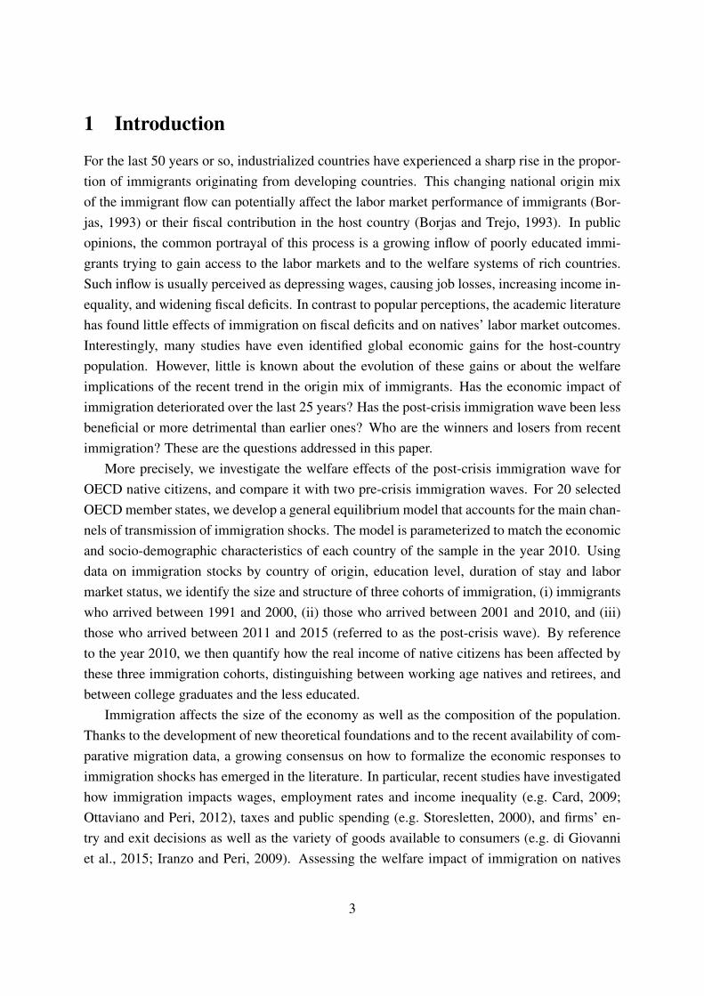
Abstract We investigate the welfare implications of two pre-crisis immigration waves (1991–2000 and 2001–2010) and of the post-crisis wave (2011–2015) for OECD native citizens. To do so, we develop a general equilibrium model that accounts for the main channels of transmission of immigration shocks – the employment and wage effects, the fiscal effect, and the market size effect – and for the interactions between them. We parameterize our model for 20 selected OECD member states. We find that the three waves induce positive effects on the real income of natives, however the size of these gains varies considerably across countries and across skill groups. In relative terms, the post-crisis wave induces smaller welfare gains compared to the previous ones. This is due to the changing origin mix of immigrants, which translates into lower levels of human capital and smaller fiscal gains. However, differences across cohorts explain a tiny fraction of the highly persistent, cross-country heterogeneity in the economic benefits from immigration.

KeywordsImmigration, Welfare, Crisis, Inequality, General Equilibrium.

JELC68, F22, J24.

CEPII (Centre d’Etudes Prospectives et d’Informations Internationales) is a French institute dedicated to producing independent, policy-oriented economic research helpful to understand the international economic environment and challenges in the areas of trade policy, competitiveness, macroeconomics, international finance and growth.

CEPII Working PaperContributing to research in international economics

© CEPII, PARIS, 2018

All rights reserved. Opinions expressed in this publication are those of the author(s) alone.

Editorial Director: Sébastien Jean

Production: Laure Boivin

No ISSN: 1293-2574

CEPII20, avenue de SégurTSA 1072675334 Paris Cedex 07+33 1 53 68 55 00www.cepii.frPress contact: presse@cepii.fr

Working Paper

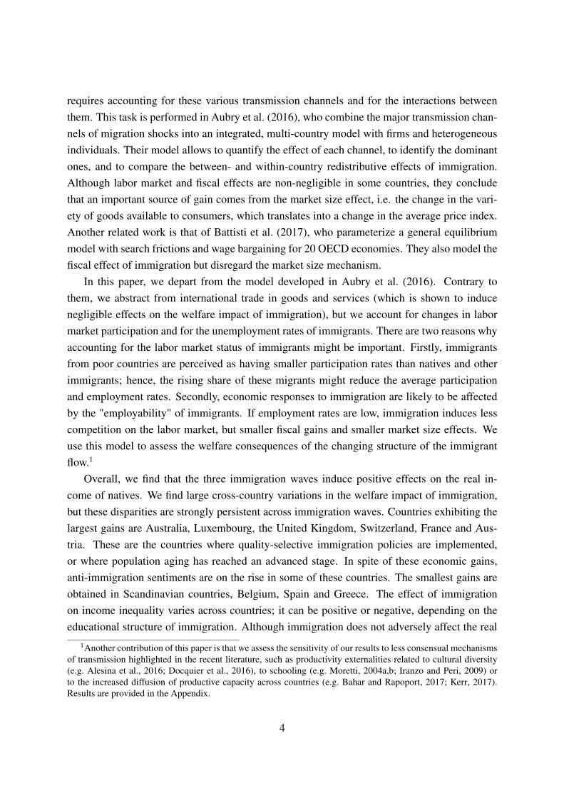
1 Introduction

For the last 50 years or so, industrialized countries have experienced a sharp rise in the propor-tion of immigrants originating from developing countries. This changing national origin mixof the immigrant flow can potentially affect the labor market performance of immigrants (Bor-jas, 1993) or their fiscal contribution in the host country (Borjas and Trejo, 1993). In publicopinions, the common portrayal of this process is a growing inflow of poorly educated immi-grants trying to gain access to the labor markets and to the welfare systems of rich countries.Such inflow is usually perceived as depressing wages, causing job losses, increasing income in-equality, and widening fiscal deficits. In contrast to popular perceptions, the academic literaturehas found little effects of immigration on fiscal deficits and on natives’ labor market outcomes.Interestingly, many studies have even identified global economic gains for the host-countrypopulation. However, little is known about the evolution of these gains or about the welfareimplications of the recent trend in the origin mix of immigrants. Has the economic impact ofimmigration deteriorated over the last 25 years? Has the post-crisis immigration wave been lessbeneficial or more detrimental than earlier ones? Who are the winners and losers from recentimmigration? These are the questions addressed in this paper.

More precisely, we investigate the welfare effects of the post-crisis immigration wave forOECD native citizens, and compare it with two pre-crisis immigration waves. For 20 selectedOECD member states, we develop a general equilibrium model that accounts for the main chan-nels of transmission of immigration shocks. The model is parameterized to match the economicand socio-demographic characteristics of each country of the sample in the year 2010. Usingdata on immigration stocks by country of origin, education level, duration of stay and labormarket status, we identify the size and structure of three cohorts of immigration, (i) immigrantswho arrived between 1991 and 2000, (ii) those who arrived between 2001 and 2010, and (iii)those who arrived between 2011 and 2015 (referred to as the post-crisis wave). By referenceto the year 2010, we then quantify how the real income of native citizens has been affected bythese three immigration cohorts, distinguishing between working age natives and retirees, andbetween college graduates and the less educated.

Immigration affects the size of the economy as well as the composition of the population.Thanks to the development of new theoretical foundations and to the recent availability of com-parative migration data, a growing consensus on how to formalize the economic responses toimmigration shocks has emerged in the literature. In particular, recent studies have investigatedhow immigration impacts wages, employment rates and income inequality (e.g. Card, 2009;Ottaviano and Peri, 2012), taxes and public spending (e.g. Storesletten, 2000), and firms’ en-try and exit decisions as well as the variety of goods available to consumers (e.g. di Giovanniet al., 2015; Iranzo and Peri, 2009). Assessing the welfare impact of immigration on natives

3

requires accounting for these various transmission channels and for the interactions betweenthem. This task is performed in Aubry et al. (2016), who combine the major transmission chan-nels of migration shocks into an integrated, multi-country model with firms and heterogeneousindividuals. Their model allows to quantify the effect of each channel, to identify the dominantones, and to compare the between- and within-country redistributive effects of immigration.Although labor market and fiscal effects are non-negligible in some countries, they concludethat an important source of gain comes from the market size effect, i.e. the change in the vari-ety of goods available to consumers, which translates into a change in the average price index.Another related work is that of Battisti et al. (2017), who parameterize a general equilibriummodel with search frictions and wage bargaining for 20 OECD economies. They also model thefiscal effect of immigration but disregard the market size mechanism.

In this paper, we depart from the model developed in Aubry et al. (2016). Contrary tothem, we abstract from international trade in goods and services (which is shown to inducenegligible effects on the welfare impact of immigration), but we account for changes in labormarket participation and for the unemployment rates of immigrants. There are two reasons whyaccounting for the labor market status of immigrants might be important. Firstly, immigrantsfrom poor countries are perceived as having smaller participation rates than natives and otherimmigrants; hence, the rising share of these migrants might reduce the average participationand employment rates. Secondly, economic responses to immigration are likely to be affectedby the "employability" of immigrants. If employment rates are low, immigration induces lesscompetition on the labor market, but smaller fiscal gains and smaller market size effects. Weuse this model to assess the welfare consequences of the changing structure of the immigrantflow.1

Overall, we find that the three immigration waves induce positive effects on the real in-come of natives. We find large cross-country variations in the welfare impact of immigration,but these disparities are strongly persistent across immigration waves. Countries exhibiting thelargest gains are Australia, Luxembourg, the United Kingdom, Switzerland, France and Aus-tria. These are the countries where quality-selective immigration policies are implemented,or where population aging has reached an advanced stage. In spite of these economic gains,anti-immigration sentiments are on the rise in some of these countries. The smallest gains areobtained in Scandinavian countries, Belgium, Spain and Greece. The effect of immigrationon income inequality varies across countries; it can be positive or negative, depending on theeducational structure of immigration. Although immigration does not adversely affect the real

1Another contribution of this paper is that we assess the sensitivity of our results to less consensual mechanismsof transmission highlighted in the recent literature, such as productivity externalities related to cultural diversity(e.g. Alesina et al., 2016; Docquier et al., 2016), to schooling (e.g. Moretti, 2004a,b; Iranzo and Peri, 2009) orto the increased diffusion of productive capacity across countries (e.g. Bahar and Rapoport, 2017; Kerr, 2017).Results are provided in the Appendix.

4

income of less educated natives, it increases the income gap with college graduates in a majorityof countries (especially in Scandinavian countries, Belgium, Spain and Greece).

Turning our attention to the evolution of these gains, our analysis reveals that the changingorigin mix is a good predictor of the changing educational structure of the immigrant popula-tion. This implies that the structure of dyadic migrant inflows is highly persistent over time.However, with a few exceptions, the correlation between dyadic and source-country character-istics is limited. This means that (i) the actual "education mix" of immigrant flows is affected bythe origin mix through dyadic self-selection patterns, and (ii) these dyadic differences in self-selection are highly persistent across immigrant waves. They presumably vary with enduringdestination characteristics such as immigration policy, geography, language, colonial ties, wageand industry structures, etc. Selection along labor market preferences is driven by a subset ofthese characteristics as well as by labor market institutions. As far as welfare implications areconcerned, we find no evidence of systematic changes across the two pre-crisis immigrationwaves. On the contrary, the post-crisis wave induces smaller welfare gains compared to theearlier ones. This is because post-crisis immigrants are relatively less educated than formerimmigrants. They earn less and induce smaller fiscal gains. With the exception of Portugal, thisresult applies to all 20 OECD countries under investigation. The inequality impact has slightlyintensified after the crisis, but not in all countries. These phenomena can be attributed to thecombined effect of the changing origin mix and of self-selection. However, as stated above,these welfare changes induced by the origin mix are limited and much smaller than those in-duced by highly persistent self-selection patterns. In other words, over the last 25 years, thewelfare responses to the changing origin mix have been limited.

The remainder of the paper is organized as follows. Section 2 provides stylized facts on thechanging size and structure of immigration as well as on the process of migrants’ self-selection.Section 3 describes the theoretical model and the calibration strategy. Quantitative results arediscussed in Section 4. Finally, Section 5 concludes.

2 Origin mix and self-selection: stylized facts

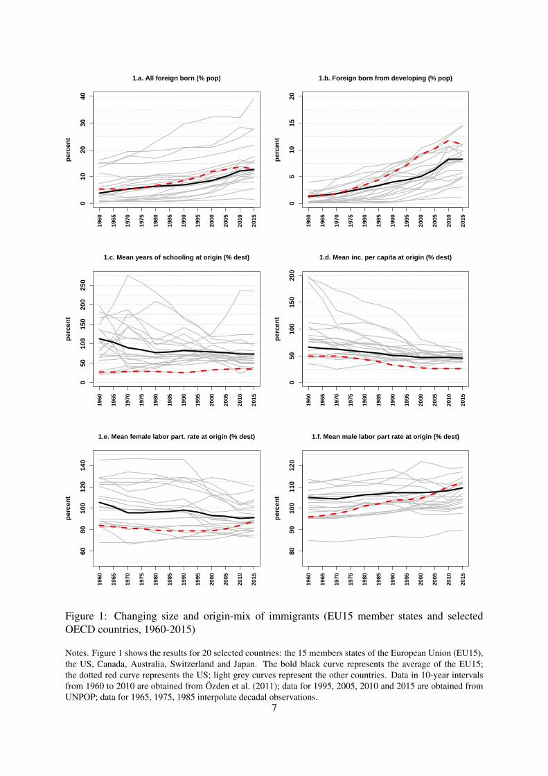
Immigration has become a first-order political issue in virtually all industrialized countries. Thisis partly due to the fact that the size and structure of immigration have considerably evolvedover the last half century. This is illustrated in Figure 1, which depicts immigration trendsto 20 selected OECD countries, namely the 15 members of the European Union (EU15), theUS, Canada, Australia, Switzerland and Japan. Exploiting bilateral migration data from Özdenet al. (2011) and from United Nations (2014), Figure 1.a shows that the share of the foreign-born population increased in all high-income countries between 1960 and 2015; on average, itincreased from 4.6 to 11.0 percent (+6.4 percentage points). Figure 1.b shows that this change is

5

totally explained by the inflow of immigrants from developing countries, whose average sharein the total population increased from 1.5 to 7.9 percent (once again, +6.4 percentage points).In spite of limited differences across countries, an increasing share of the population of OECDmember states is originating from countries that are economically, geographically and culturallymore distant. In the US (red bold curve), the population share of immigrants from developingcountries increased by 9.6% (1.3 times the change in the total immigration rate); in the EU15(black bold curve), it increased by 7.1% (83% of the total change). The growth rate of the totalstock of immigrants has been curbed by the recent crisis. However, the crisis has affected bothinflows from rich and from poor countries.

In this context, the rising concerns about immigration are legitimate. Developing countriesexhibit lower productivity levels, lower levels of human capital, and lower labor market par-ticipation rates (mostly due to lower female participation rates). The changing origin mix ofimmigrant flows is thus usually associated with a decrease in their average skill level, produc-tivity, and participation rate. Figures 1.c to 1.f provide the mean gaps in schooling, income, andlabor market participation between origin and destination countries, as proxied by the ratio ofthe (weighted) mean level observed in migrants’ origin countries to the mean level observed inthe destination country. A ratio above 100 percent means that the average immigrant is orig-inating from a country with more schooling, higher income per capita or higher participationrates; a ratio below 100 percent means that immigrants have observable characteristics asso-ciated with lower productivity. Between 1960 and 2015, the schooling ratio decreased in themajority of countries (except in the US, Australia, Canada, Switzerland, and to a lesser extentJapan, Belgium and Portugal). It increased from 27 to 35 in the US; it decreased from 112 to 73in the EU15 (see Figure 1.c). Over the same period, the income ratio decreased in all countries.It declined from 50 to 26 in the US and from 66 to 46 in the EU15 (see Figure 1.d). Finally,while males’ participation rates are usually greater at origin (see Figure 1.f), females’ participa-tion rates declined in virtually all countries (except in the US and in Japan). It increased from84 to 88 in the US, and decreased from 105 to 91 in the EU15 (see Figure 1.e).

Under neutral selection, the changing origin mix of immigrant flows would result in largechanges in the educational structure, productivity and labor market performance of immigrants.Natives’ views reflect these presumptions. For example, the 2014 edition of the TransatlanticTrends on Immigration reveals that about 60 percent of European citizens view emigration andimmigration as a problem and not as an opportunity. Such concerns are particularly importantregarding immigrants from developing countries; 56 percent of Europeans expressed concernsabout non-EU immigration, while only 43 percent perceive intra-EU migration as a problem.Public opinions are partly governed by non-economic reasons such as the perceived negativeeffects of immigration on social cohesiveness, national identity, crime, terrorism, etc. However,attitudes towards immigration are systematically correlated with two major economic concerns:

6

010

2030

40

perc

ent

1.a. All foreign born (% pop)

1960

1965

1970

1975

1980

1985

1990

1995

2000

2005

2010

2015

05

1015

20

perc

ent

1.b. Foreign born from developing (% pop)

1960

1965

1970

1975

1980

1985

1990

1995

2000

2005

2010

2015

050

100

150

200

250

perc

ent

1.c. Mean years of schooling at origin (% dest)

1960

1965

1970

1975

1980

1985

1990

1995

2000

2005

2010

2015

050

100

150

200

perc

ent

1.d. Mean inc. per capita at origin (% dest)

1960

1965

1970

1975

1980

1985

1990

1995

2000

2005

2010

2015

6080

100

120

140

perc

ent

1.e. Mean female labor part. rate at origin (% dest)

1960

1965

1970

1975

1980

1985

1990

1995

2000

2005

2010

2015

8090

100

110

120

perc

ent

1.f. Mean male labor part rate at origin (% dest)

1960

1965

1970

1975

1980

1985

1990

1995

2000

2005

2010

2015

Figure 1: Changing size and origin-mix of immigrants (EU15 member states and selectedOECD countries, 1960-2015)

Notes. Figure 1 shows the results for 20 selected countries: the 15 members states of the European Union (EU15),the US, Canada, Australia, Switzerland and Japan. The bold black curve represents the average of the EU15;the dotted red curve represents the US; light grey curves represent the other countries. Data in 10-year intervalsfrom 1960 to 2010 are obtained from Özden et al. (2011); data for 1995, 2005, 2010 and 2015 are obtained fromUNPOP; data for 1965, 1975, 1985 interpolate decadal observations.

7

the perceived adverse labor market effects of immigration, and its fiscal effects. The EuropeanSocial Survey data for the year 2014 show that only 26 percent of European respondents be-lieve that immigrants contribute positively to public finances, and only 35.9 percent think thatimmigrants contribute to create new jobs for natives.2

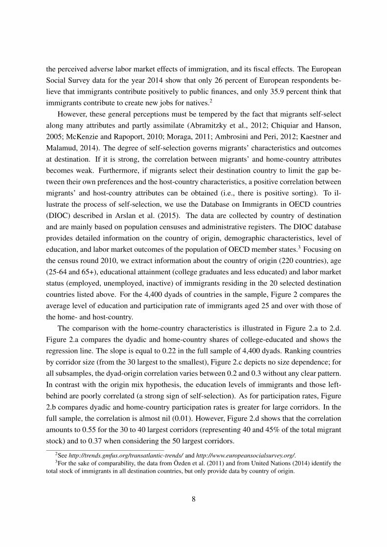
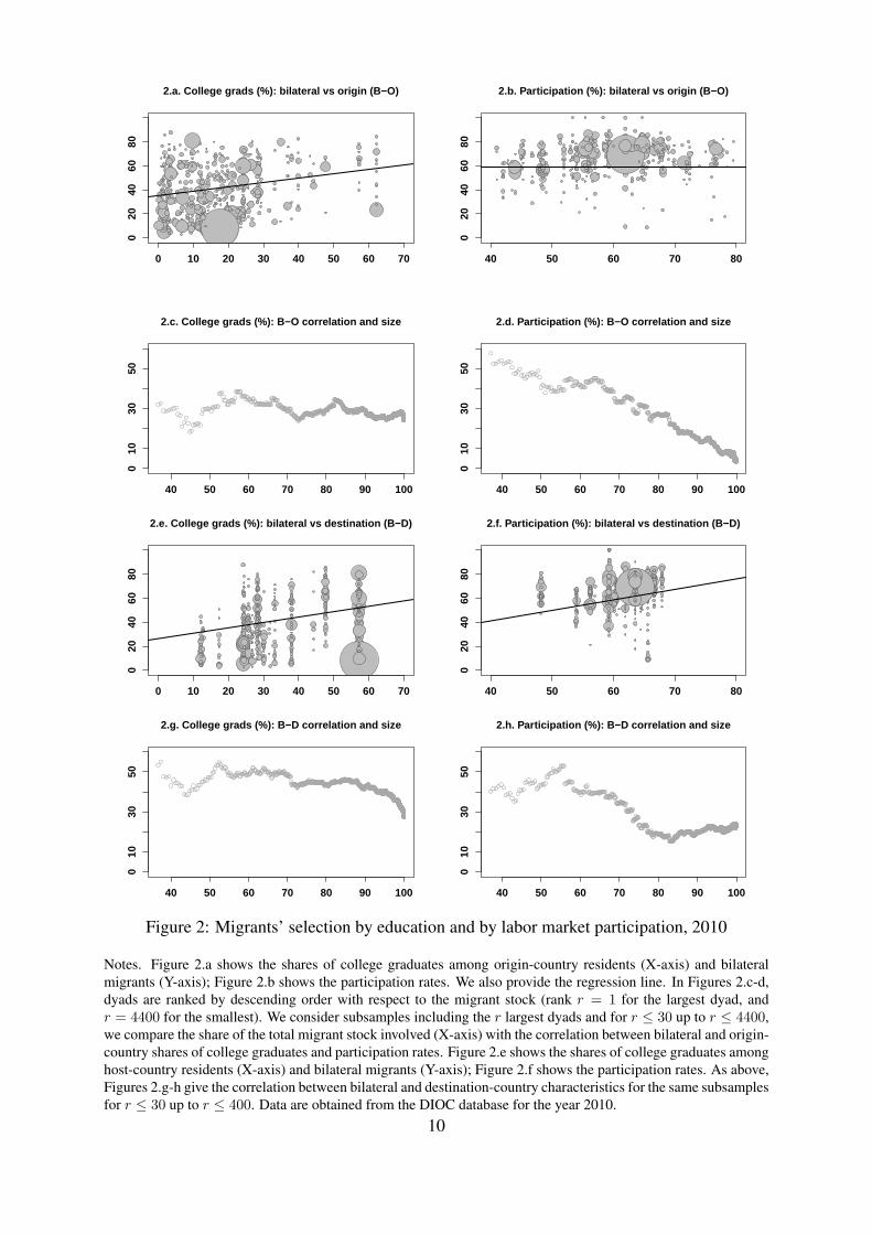
However, these general perceptions must be tempered by the fact that migrants self-selectalong many attributes and partly assimilate (Abramitzky et al., 2012; Chiquiar and Hanson,2005; McKenzie and Rapoport, 2010; Moraga, 2011; Ambrosini and Peri, 2012; Kaestner andMalamud, 2014). The degree of self-selection governs migrants’ characteristics and outcomesat destination. If it is strong, the correlation between migrants’ and home-country attributesbecomes weak. Furthermore, if migrants select their destination country to limit the gap be-tween their own preferences and the host-country characteristics, a positive correlation betweenmigrants’ and host-country attributes can be obtained (i.e., there is positive sorting). To il-lustrate the process of self-selection, we use the Database on Immigrants in OECD countries(DIOC) described in Arslan et al. (2015). The data are collected by country of destinationand are mainly based on population censuses and administrative registers. The DIOC databaseprovides detailed information on the country of origin, demographic characteristics, level ofeducation, and labor market outcomes of the population of OECD member states.3 Focusing onthe census round 2010, we extract information about the country of origin (220 countries), age(25-64 and 65+), educational attainment (college graduates and less educated) and labor marketstatus (employed, unemployed, inactive) of immigrants residing in the 20 selected destinationcountries listed above. For the 4,400 dyads of countries in the sample, Figure 2 compares theaverage level of education and participation rate of immigrants aged 25 and over with those ofthe home- and host-country.

The comparison with the home-country characteristics is illustrated in Figure 2.a to 2.d.Figure 2.a compares the dyadic and home-country shares of college-educated and shows theregression line. The slope is equal to 0.22 in the full sample of 4,400 dyads. Ranking countriesby corridor size (from the 30 largest to the smallest), Figure 2.c depicts no size dependence; forall subsamples, the dyad-origin correlation varies between 0.2 and 0.3 without any clear pattern.In contrast with the origin mix hypothesis, the education levels of immigrants and those left-behind are poorly correlated (a strong sign of self-selection). As for participation rates, Figure2.b compares dyadic and home-country participation rates is greater for large corridors. In thefull sample, the correlation is almost nil (0.01). However, Figure 2.d shows that the correlationamounts to 0.55 for the 30 to 40 largest corridors (representing 40 and 45% of the total migrantstock) and to 0.37 when considering the 50 largest corridors.

2See http://trends.gmfus.org/transatlantic-trends/ and http://www.europeansocialsurvey.org/.3For the sake of comparability, the data from Özden et al. (2011) and from United Nations (2014) identify the

total stock of immigrants in all destination countries, but only provide data by country of origin.

8

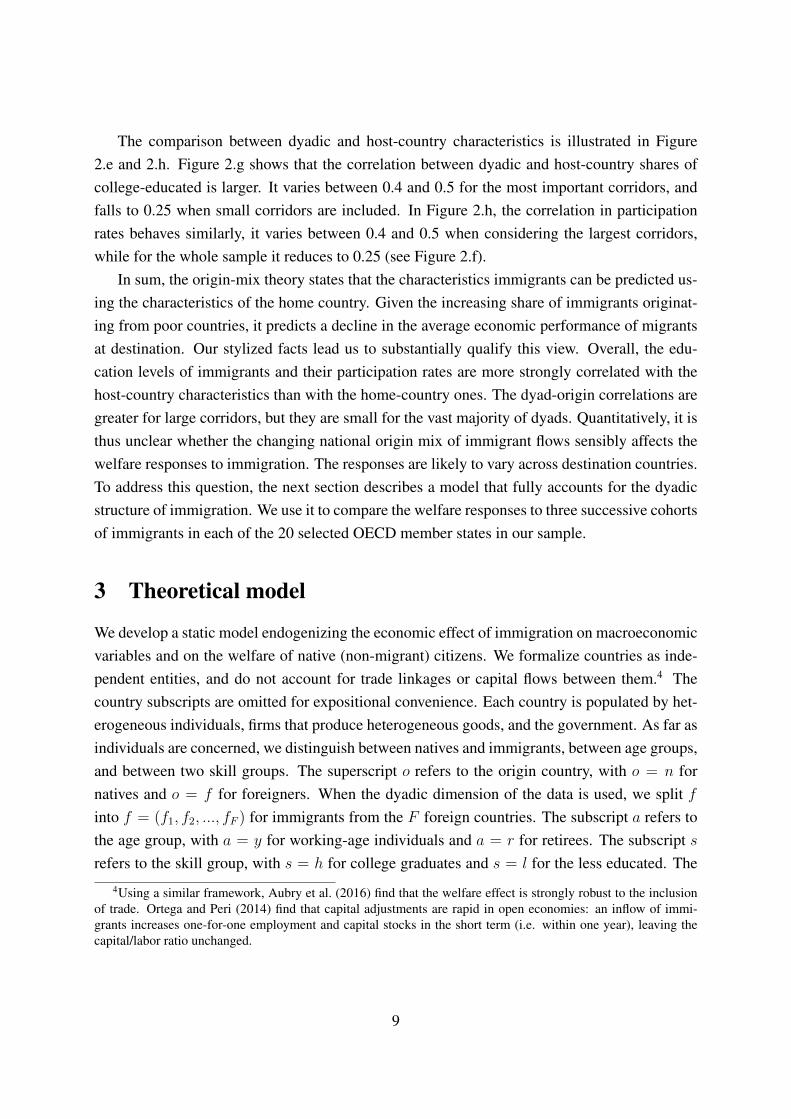
The comparison between dyadic and host-country characteristics is illustrated in Figure2.e and 2.h. Figure 2.g shows that the correlation between dyadic and host-country shares ofcollege-educated is larger. It varies between 0.4 and 0.5 for the most important corridors, andfalls to 0.25 when small corridors are included. In Figure 2.h, the correlation in participationrates behaves similarly, it varies between 0.4 and 0.5 when considering the largest corridors,while for the whole sample it reduces to 0.25 (see Figure 2.f).

In sum, the origin-mix theory states that the characteristics immigrants can be predicted us-ing the characteristics of the home country. Given the increasing share of immigrants originat-ing from poor countries, it predicts a decline in the average economic performance of migrantsat destination. Our stylized facts lead us to substantially qualify this view. Overall, the edu-cation levels of immigrants and their participation rates are more strongly correlated with thehost-country characteristics than with the home-country ones. The dyad-origin correlations aregreater for large corridors, but they are small for the vast majority of dyads. Quantitatively, it isthus unclear whether the changing national origin mix of immigrant flows sensibly affects thewelfare responses to immigration. The responses are likely to vary across destination countries.To address this question, the next section describes a model that fully accounts for the dyadicstructure of immigration. We use it to compare the welfare responses to three successive cohortsof immigrants in each of the 20 selected OECD member states in our sample.

3 Theoretical model

We develop a static model endogenizing the economic effect of immigration on macroeconomicvariables and on the welfare of native (non-migrant) citizens. We formalize countries as inde-pendent entities, and do not account for trade linkages or capital flows between them.4 Thecountry subscripts are omitted for expositional convenience. Each country is populated by het-erogeneous individuals, firms that produce heterogeneous goods, and the government. As far asindividuals are concerned, we distinguish between natives and immigrants, between age groups,and between two skill groups. The superscript o refers to the origin country, with o = n fornatives and o = f for foreigners. When the dyadic dimension of the data is used, we split finto f = (f1, f2, ..., fF ) for immigrants from the F foreign countries. The subscript a refers tothe age group, with a = y for working-age individuals and a = r for retirees. The subscript srefers to the skill group, with s = h for college graduates and s = l for the less educated. The

4Using a similar framework, Aubry et al. (2016) find that the welfare effect is strongly robust to the inclusionof trade. Ortega and Peri (2014) find that capital adjustments are rapid in open economies: an inflow of immi-grants increases one-for-one employment and capital stocks in the short term (i.e. within one year), leaving thecapital/labor ratio unchanged.

9

0 10 20 30 40 50 60 70

020

4060

80

2.a. College grads (%): bilateral vs origin (B−O)

40 50 60 70 80

020

4060

80

2.b. Participation (%): bilateral vs origin (B−O)

40 50 60 70 80 90 100

010

3050

2.c. College grads (%): B−O correlation and size

40 50 60 70 80 90 100

010

3050

2.d. Participation (%): B−O correlation and size

0 10 20 30 40 50 60 70

020

4060

80

2.e. College grads (%): bilateral vs destination (B−D)

40 50 60 70 80

020

4060

80

2.f. Participation (%): bilateral vs destination (B−D)

40 50 60 70 80 90 100

010

3050

2.g. College grads (%): B−D correlation and size

40 50 60 70 80 90 100

010

3050

2.h. Participation (%): B−D correlation and size

Figure 2: Migrants’ selection by education and by labor market participation, 2010

Notes. Figure 2.a shows the shares of college graduates among origin-country residents (X-axis) and bilateralmigrants (Y-axis); Figure 2.b shows the participation rates. We also provide the regression line. In Figures 2.c-d,dyads are ranked by descending order with respect to the migrant stock (rank r = 1 for the largest dyad, andr = 4400 for the smallest). We consider subsamples including the r largest dyads and for r ≤ 30 up to r ≤ 4400,we compare the share of the total migrant stock involved (X-axis) with the correlation between bilateral and origin-country shares of college graduates and participation rates. Figure 2.e shows the shares of college graduates amonghost-country residents (X-axis) and bilateral migrants (Y-axis); Figure 2.f shows the participation rates. As above,Figures 2.g-h give the correlation between bilateral and destination-country characteristics for the same subsamplesfor r ≤ 30 up to r ≤ 400. Data are obtained from the DIOC database for the year 2010.

10

demographic size of these groups is denoted byN oa,s and is assumed to be exogenous.5 As far as

firms are concerned, there is a mass B of firms that operate on a monopolistically competitivemarket with a fixed cost of entry, each of them produces a differentiated good. The governmenttaxes income and consumption to finance redistributive transfers, unemployment benefits andpublic consumption.

In line with the recent literature, four channels of transmission of immigration shocks aretaken into consideration in the benchmark model: the employment effect, the wage effect, thefiscal effect, and the market size effect. Additional and less consensual channels are investigatedin the robustness analysis in the Appendix. We model the labor market effects as in Ottavianoand Peri (2012), the fiscal effect as in Storesletten (2000), the market-size effect as in Krugman(1980). We account for the age structure of immigration to match the fiscal features of eacheconomy. In addition, we account for the difference in employment rates between immigrantsand natives by introducing heterogeneity in the disutility of labor and in unemployment rates.Note that these could as well reflect differential access to jobs due to discrimination. The datareveal that differences in employment rates are mainly governed by differences in participationrates. This motivates our choice to endogenize participation rates and to assume, for simplicity,that active workers spend an exogenous fraction of their active time in unemployment (due,for example, to exogenous job destruction and finding rates).6 Accounting for immigrants’employment is important as it governs the intensity of the competition with natives on the labormarket and well as the size of fiscal and market size effects.

In this section, we describe the preferences and the technology used to endogenize individ-uals’ and firms’ decisions in Sections 3.1 and 3.2. We then characterize the monopolisticallycompetitive equilibrium in Section 3.4. Finally, we explain our parameterization strategy inSection 3.5.

3.1 Individuals

The preferences of a representative individual in the age group a = (y, r), of education levels = (h, l) and from origin country o = (n, f) are described by the following utility function:

Uoa,s = Coa,s −

φoa,s(1− γoa,s)1+η

1 + η. (1)

5In the real world, the population structure in general, and immigration rates in particular, depend on the stateof the economy. As we are interested in the "causal" impact of immigration on the welfare of natives, our strategyconsists of (i) endogenizing the state of the economy as a function of the size and structure of immigration, (ii)calibrating our model using observed immigration data, and (iii) using counterfactual no-immigration scenarios toquantify the welfare impact of immigration.

6Note that Battisti et al. (2017) use a different model with exogenous participation rates and endogenous un-employment rates. In the sensitivity analysis in Appendix, we show that our results are robust to alternativeunemployment assumptions.

11

Utility is a linear function of a composite consumption aggregate, Coa,s (discussed below) and

depends negatively on the endogenous amount of time spent on the labor market, 1 − γoa,s.Hence, the supply of labor in the group (o, a, s) is defined as (1 − γoa,s)N o

a,s. The parameter ηis the inverse of the elasticity of labor supply to labor income; it is common to all individuals.The parameter φoa,s captures the disutility of participating in the labor market (i.e. disutility ofworking or of searching for a job). It varies by age group, by education level and by countryof origin. We assume φor,s = ∞ for all retirees, implying that retirees are inactive and onlyconsume the transfers received from the government. As far as working age individuals areconcerned, we calibrate φoy,s so as to match the observed participation rate in ech dyadic group.Hence, the model allows to capture differences in participation rate across skill groups andacross natives and immigrants from a specific origin country; these differences are assumedto be due to the heterogeneity in cultural traits or social norms between countries, and to thecultural selection of immigrants.

In addition, we assume that consumers have a preference for variety. This means that theutility from consumption does not only depend on the quantity of goods consumed; it alsoincreases with the variety of goods. Remember there is a mass B of varieties available forconsumption. Following Krugman (1980), the utility of consumption is described by a CESutility function over the continuum of varieties:

Coa,s =

[∫ B

0

coa,s(i)ε−1ε di

] εε−1

, (2)

where coa,s(i) stands for the quantity of variety i ∈ [0, B] produced in the country and consumedby an individual of type (a, o, s). Varieties are imperfect substitutes, characterized by a constantelasticity of substitution equal to ε > 1.

In each destination country, working age immigrants in a given skill group are perfectlysubstitutable workers from the firm’s perspective. They have identical marginal productivitylevels and earn identical wages per hour worked, wfs ,∀f = (f1, f2, ..., fF ), which usually differsfrom the native’s wage rate, wns . At each moment in time, active workers face exogenousjob separation and finding rates, implying that they spend an exogenous fraction 1 − uos oftheir active time in employment, and the remaining fraction uos in unemployment (searchingfor a job). Working and searching induce the same disutility. Job separation and finding ratesdiffer across natives and immigrants, but are homogeneous among immigrants (i.e., ufs , ∀f =

{f1, f2, ..., fF}, and uns for natives). During each unemployment spell, active workers receiveunemployment benefits, bos, that are assumed to be proportional to their wage rate. We write bos =

δwos where δ captures the replacement rate of the national unemployment insurance scheme.Finally, the government allocates group-specific transfers to each group of individuals, T oa,s,that do not depend on the labor market status. In practice, T oa,s includes redistributive transfers

12

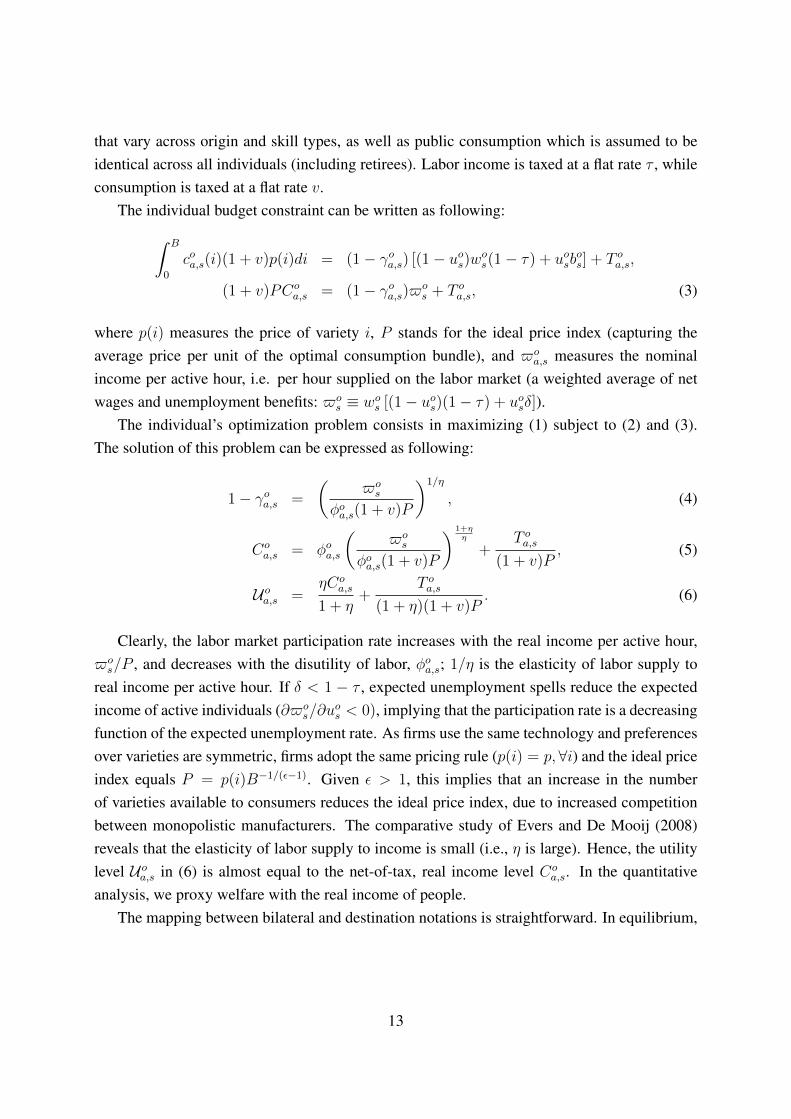
that vary across origin and skill types, as well as public consumption which is assumed to beidentical across all individuals (including retirees). Labor income is taxed at a flat rate τ , whileconsumption is taxed at a flat rate v.

The individual budget constraint can be written as following:∫ B

0

coa,s(i)(1 + v)p(i)di = (1− γoa,s) [(1− uos)wos(1− τ) + uosbos] + T oa,s,

(1 + v)PCoa,s = (1− γoa,s)$o

s + T oa,s, (3)

where p(i) measures the price of variety i, P stands for the ideal price index (capturing theaverage price per unit of the optimal consumption bundle), and $o

a,s measures the nominalincome per active hour, i.e. per hour supplied on the labor market (a weighted average of netwages and unemployment benefits: $o

s ≡ wos [(1− uos)(1− τ) + uosδ]).The individual’s optimization problem consists in maximizing (1) subject to (2) and (3).

The solution of this problem can be expressed as following:

1− γoa,s =

($os

φoa,s(1 + v)P

)1/η

, (4)

Coa,s = φoa,s

($os

φoa,s(1 + v)P

) 1+ηη

+T oa,s

(1 + v)P, (5)

Uoa,s =ηCo

a,s

1 + η+

T oa,s(1 + η)(1 + v)P

. (6)

Clearly, the labor market participation rate increases with the real income per active hour,$os/P , and decreases with the disutility of labor, φoa,s; 1/η is the elasticity of labor supply to

real income per active hour. If δ < 1 − τ , expected unemployment spells reduce the expectedincome of active individuals (∂$o

s/∂uos < 0), implying that the participation rate is a decreasing

function of the expected unemployment rate. As firms use the same technology and preferencesover varieties are symmetric, firms adopt the same pricing rule (p(i) = p, ∀i) and the ideal priceindex equals P = p(i)B−1/(ε−1). Given ε > 1, this implies that an increase in the numberof varieties available to consumers reduces the ideal price index, due to increased competitionbetween monopolistic manufacturers. The comparative study of Evers and De Mooij (2008)reveals that the elasticity of labor supply to income is small (i.e., η is large). Hence, the utilitylevel Uoa,s in (6) is almost equal to the net-of-tax, real income level Co

a,s. In the quantitativeanalysis, we proxy welfare with the real income of people.

The mapping between bilateral and destination notations is straightforward. In equilibrium,

13

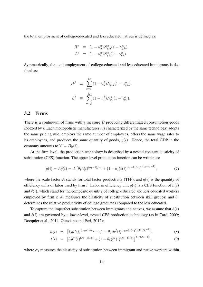
the total employment of college-educated and less educated natives is defined as:

Hn ≡ (1− unh)Nny,h(1− γny,h),

Ln ≡ (1− unl )Nny,l(1− γny,l).

Symmetrically, the total employment of college-educated and less educated immigrants is de-fined as:

Hf ≡fF∑o=f1

(1− ufh)Noy,h(1− γoy,h),

Lf ≡fF∑o=f1

(1− ufl )Noy,l(1− γoy,l).

3.2 Firms

There is a continuum of firms with a measure B producing differentiated consumption goodsindexed by i. Each monopolistic manufacturer i is characterized by the same technology, adoptsthe same pricing rule, employs the same number of employees, offers the same wage rates toits employees, and produces the same quantity of goods, y(i). Hence, the total GDP in theeconomy amounts to Y = By(i).

At the firm level, the production technology is described by a nested constant elasticity ofsubstitution (CES) function. The upper-level production function can be written as:

y(i) = Aq(i) = A[θ1h(i)(σ1−1)/σ1 + (1− θ1)`(i)(σ1−1)/σ1

]σ1/(σ1−1), (7)

where the scale factor A stands for total factor productivity (TFP), and q(i) is the quantity ofefficiency units of labor used by firm i. Labor in efficiency unit q(i) is a CES function of h(i)

and `(i), which stand for the composite quantity of college-educated and less educated workersemployed by firm i; σ1 measures the elasticity of substitution between skill groups; and θ1

determines the relative productivity of college graduates compared to the less educated.To capture the imperfect substitution between immigrants and natives, we assume that h(i)

and `(i) are governed by a lower-level, nested CES production technology (as in Card, 2009;Docquier et al., 2014; Ottaviano and Peri, 2012):

h(i) =[θ2h

n(i)(σ2−1)/σ2 + (1− θ2)hf (i)(σ2−1)/σ2]σ2/(σ2−1)

, (8)

`(i) =[θ2`

n(i)(σ2−1)/σ2 + (1− θ2)`f (i)(σ2−1)/σ2]σ2/(σ2−1)

, (9)

where σ2 measures the elasticity of substitution between immigrant and native workers within

14

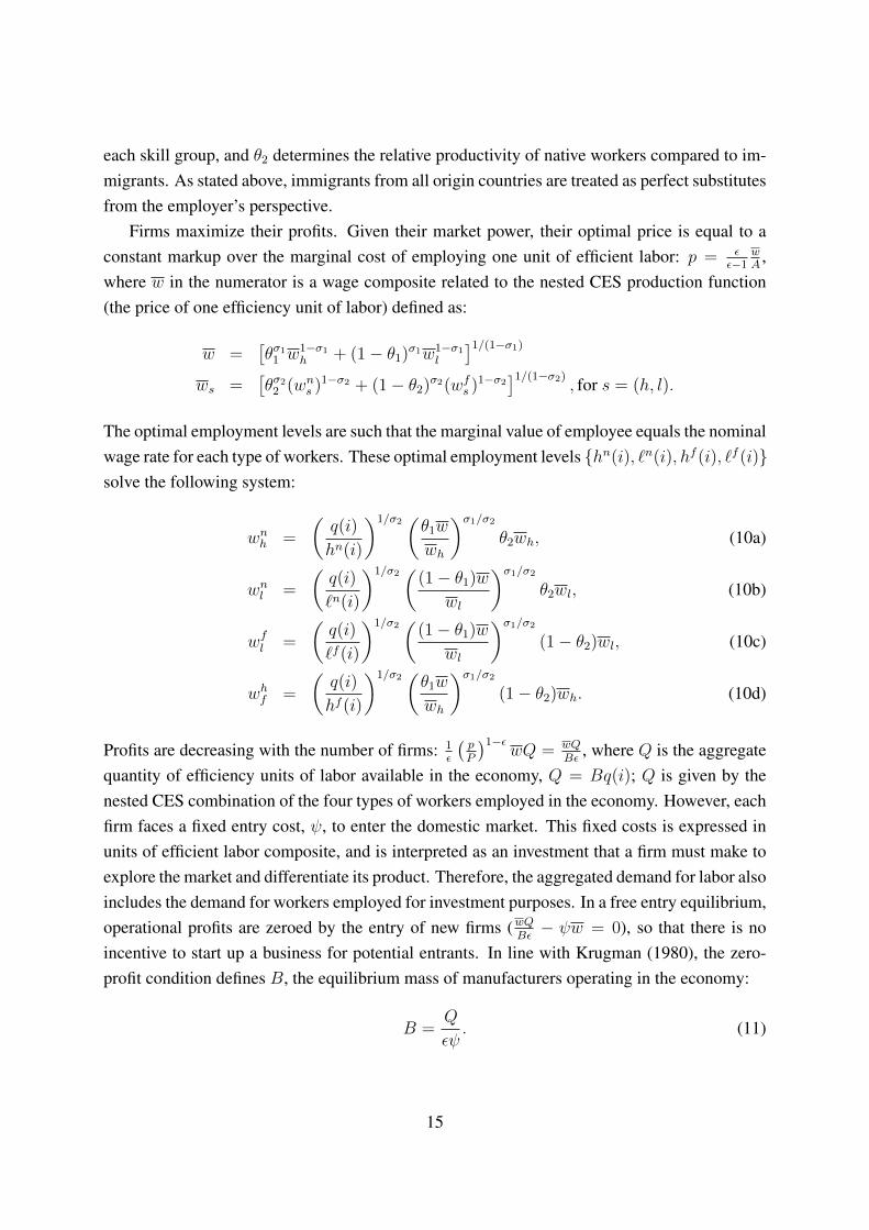
each skill group, and θ2 determines the relative productivity of native workers compared to im-migrants. As stated above, immigrants from all origin countries are treated as perfect substitutesfrom the employer’s perspective.

Firms maximize their profits. Given their market power, their optimal price is equal to aconstant markup over the marginal cost of employing one unit of efficient labor: p = ε

ε−1wA

,where w in the numerator is a wage composite related to the nested CES production function(the price of one efficiency unit of labor) defined as:

w =[θσ11 w

1−σ1h + (1− θ1)σ1w1−σ1

l

]1/(1−σ1)ws =

[θσ22 (wns )1−σ2 + (1− θ2)σ2(wfs )1−σ2

]1/(1−σ2), for s = (h, l).

The optimal employment levels are such that the marginal value of employee equals the nominalwage rate for each type of workers. These optimal employment levels {hn(i), `n(i), hf (i), `f (i)}solve the following system:

wnh =

(q(i)

hn(i)

)1/σ2 (θ1wwh

)σ1/σ2θ2wh, (10a)

wnl =

(q(i)

`n(i)

)1/σ2 ((1− θ1)wwl

)σ1/σ2θ2wl, (10b)

wfl =

(q(i)

`f (i)

)1/σ2 ((1− θ1)wwl

)σ1/σ2(1− θ2)wl, (10c)

whf =

(q(i)

hf (i)

)1/σ2 (θ1wwh

)σ1/σ2(1− θ2)wh. (10d)

Profits are decreasing with the number of firms: 1ε

(pP

)1−εwQ = wQ

Bε, where Q is the aggregate

quantity of efficiency units of labor available in the economy, Q = Bq(i); Q is given by thenested CES combination of the four types of workers employed in the economy. However, eachfirm faces a fixed entry cost, ψ, to enter the domestic market. This fixed costs is expressed inunits of efficient labor composite, and is interpreted as an investment that a firm must make toexplore the market and differentiate its product. Therefore, the aggregated demand for labor alsoincludes the demand for workers employed for investment purposes. In a free entry equilibrium,operational profits are zeroed by the entry of new firms (wQ

Bε− ψw = 0), so that there is no

incentive to start up a business for potential entrants. In line with Krugman (1980), the zero-profit condition defines B, the equilibrium mass of manufacturers operating in the economy:

B =Q

εψ. (11)

15

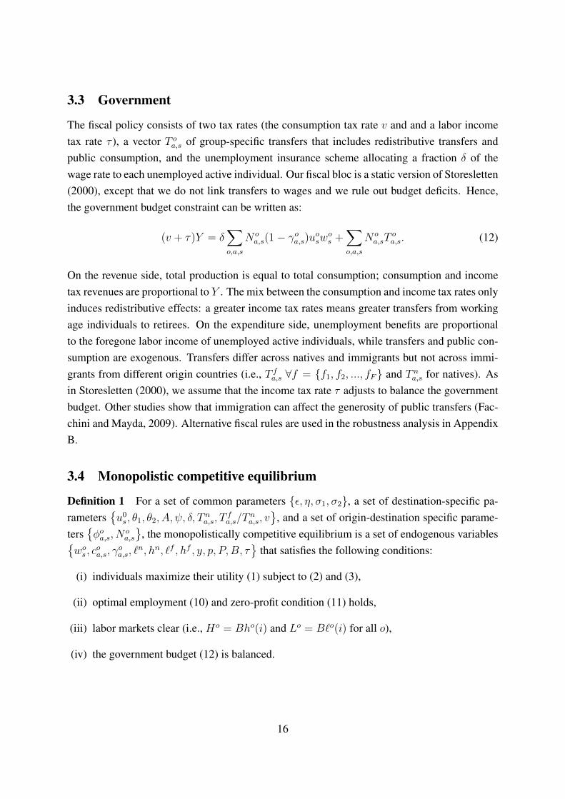
3.3 Government

The fiscal policy consists of two tax rates (the consumption tax rate v and and a labor incometax rate τ ), a vector T oa,s of group-specific transfers that includes redistributive transfers andpublic consumption, and the unemployment insurance scheme allocating a fraction δ of thewage rate to each unemployed active individual. Our fiscal bloc is a static version of Storesletten(2000), except that we do not link transfers to wages and we rule out budget deficits. Hence,the government budget constraint can be written as:

(v + τ)Y = δ∑o,a,s

N oa,s(1− γoa,s)uoswos +

∑o,a,s

N oa,sT

oa,s. (12)

On the revenue side, total production is equal to total consumption; consumption and incometax revenues are proportional to Y . The mix between the consumption and income tax rates onlyinduces redistributive effects: a greater income tax rates means greater transfers from workingage individuals to retirees. On the expenditure side, unemployment benefits are proportionalto the foregone labor income of unemployed active individuals, while transfers and public con-sumption are exogenous. Transfers differ across natives and immigrants but not across immi-grants from different origin countries (i.e., T fa,s ∀f = {f1, f2, ..., fF} and T na,s for natives). Asin Storesletten (2000), we assume that the income tax rate τ adjusts to balance the governmentbudget. Other studies show that immigration can affect the generosity of public transfers (Fac-chini and Mayda, 2009). Alternative fiscal rules are used in the robustness analysis in AppendixB.

3.4 Monopolistic competitive equilibrium

Definition 1 For a set of common parameters {ε, η, σ1, σ2}, a set of destination-specific pa-rameters

{u0s, θ1, θ2, A, ψ, δ, T

na,s, T

fa,s/T

na,s, v

}, and a set of origin-destination specific parame-

ters{φoa,s, N

oa,s

}, the monopolistically competitive equilibrium is a set of endogenous variables{

wos , coa,s, γ

oa,s, `

n, hn, `f , hf , y, p, P,B, τ}

that satisfies the following conditions:

(i) individuals maximize their utility (1) subject to (2) and (3),

(ii) optimal employment (10) and zero-profit condition (11) holds,

(iii) labor markets clear (i.e., Ho = Bho(i) and Lo = B`o(i) for all o),

(iv) the government budget (12) is balanced.

16

3.5 Parameterization

Our model is parameterized to match the economic and socio-demographic characteristics of 20OECD member states (EU15 countries, the US, Australia, Canada, Japan and Switzerland) inthe year 2010. This implies matching the population structure (by age, by education, by origin),income per capita and income disparities between groups of workers, labor markets outcomes,and fiscal data. This section describes the data sources used for parameterizing the model, anddiscusses the calibration strategy. Table 1 summarizes the calibration outcomes.

Population data (N oa,s) – In line with Section 2, we use the Database on Immigrants in

OECD countries (DIOC) described in Arslan et al. (2015). For each OECD member state, thedatabase covers the census round 2010 and documents the structure of the population by countryof origin, by age, by education level, by duration of stay, and by labor market status. We firstclassify individuals by country of origin (220 countries). Immigrants reporting ex-USSR, ex-Yugoslavia or ex-Czechoslovakia as their origin country are assumed to originate from Russia,Serbia and the Czech Republic, respectively. Immigrants who did not report their origin countryare distributed proportionately to observations. Then, we define the college-educated group asindividuals who have at least one year of college education or a bachelor degree (ISCED code5). Those with no education and with pre-primary, primary or secondary education completedare defined as the less educated. We classify individuals who did not report their education levelas low-skilled. As for the age structure, we defined individuals aged 25 to 64 as the workingaged group; those aged 65 and over form the retiree population. Individuals who did not reporttheir age are assumed to belong to the working age group.

Labor force data (γoa,s, uos) – An important feature of the DIOC database is that it includes

data on the labor market status. For each origin country and each skill group, we identify theproportions of inactive, active-employed, and active-unemployed individuals aged 25 to 64. Wecan thus identify the number of employed, unemployed and inactive individuals for each skillgroup and for each country of origin.

Income data (Y,wos) – In the model, labor is the only factor of production. Hence, thenational income is equal to the national gross domestic product (GDP). Aggregate income dataare taken from OECD.Stat database; we use the level of GDP in PPP value. By definition, totalincome is the sum of wages earned by native and immigrant workers. Data on the wage ratiobetween college-educated and less educated workers are taken from the Education at Glance2012 report of the OECD; we use them as a proxy for wh/wl. Data on the wage ratio betweennative and immigrant workers are obtained from Büchel and Frick (2005) and from Docquieret al. (2014); we use them as a proxy for wns /w

fs . Using these wage ratios, employment levels

and GDP data, we can proxy the wage rate and labor income of each group.Fiscal data (v, τ, T na,s) – Comparable aggregate data on public finances are obtained from

17

the Annual National Accounts harmonized by the OECD. This database reports aggregate publicrevenues and public expenditures by broad category, as percentage of GDP. We use to identifythe consumption tax rate (v) as well as the ratio of public expenditure to GDP, which is equalto v + τ in our model. We also identify the amount of public consumption and treat it asa homogeneous transfer to all residents (as a part of T oa,s). Redistributive transfers are alsoincluded in T oa,s. In line with Aubry et al. (2016), we use the Social Expenditure Database(SOCX) of the OECD to decompose social protection expenditures, and the European UnionStatistics on Income and Living Conditions (EU-SILC, provided by Eurostat) to disaggregateeducation and social protection transfers received by the natives; we identify transfers to nativesby education level and by age group. We add these transfers to public consumption per capitaand use it as a proxy for T na,s. Finally, we also collect data on the share of unemploymentbenefits in GDP.

Calibration of common parameters (ε, σ1, σ2, η) – The model includes four common param-eters for which a consensus range of values can be found in the existing literature; benchmarkvalues are reported in the top panel of Table 1. The elasticity of substitution between varietiesof goods is estimated in the range of 3 to 8.4 by Feenstra (1994). We assume ε = 7 as a bench-mark value, which means that the model predicts conservative market size effects. As far aselasticities of substitution between groups of worker are concerned (σ1 and σ2), we follow Ot-taviano and Peri (2012) and use σ1 = 2 and σ2 = 20. Finally, we use η = 10, which impliesan elasticity of labor supply to income of 0.1, as in Evers and De Mooij (2008). We consideralternative levels in the robustness analysis (see Section B in the Appendix).

Country-specific parameters – The model also includes other parameters that vary acrosscountries to match observed economic and socio-demographic characteristics. These parame-ters capture the cross-country disparities in productivity, in fiscal policies and in labor marketinstitutions. We use all the degrees of freedom of the data to identify these parameters, dis-tinguishing between 10 sets of country-specific parameters and calibrating them to match 10sets of moments (as summarized in the bottom panel of Table 1). Consequently, our model isexactly identified. Preferences differ across types of individual. The parameter governing thedisutility of labor, φoa,s, is allowed to vary by dyad of country and by skill group. Using (4), itis calibrated to match the observed participation rate, 1− γoa,s. We obtain a matrix of 220× 20

parameters. The average level is 67% greater than the disutility parameter of American non-migrants. Exogenous unemployment rates are directly available from the DIOC data (with amean of 9.5%).

Technological parameters are also allowed to vary across countries. The firms’ preferencesfor workers are calibrated to match the wage ratios between workers. Hence, θ1 is set to matchdata on wh/wl, while θ2 matches data on wns /w

fs . The mean levels of θ1 and θ2 exceed 0.5. This

determines the aggregate quantity of labor in efficiency unit. The TFP level, A, is then chosen

18

to match the observed level of GDP in PPP value. The mean level of A is 10.5% smaller thanthe US level. As for the fixed cost of entry, ψ, we equalize it with the number of days requiredto set up a business, available from the OECD.Stat database and normalized by the US level.The scale of this variable has no impact on our results. The mean level is 43.5% greater thanthe US level.

As far as fiscal parameters are concerned, we calibrate the replacement rate δ to match theobserved share of unemployment benefits in GDP. Regarding the other public transfers, theSOCX and SILC data allow us to identify the transfer profile by age and by education levelfor natives and immigrants. However, the data for immigrants are less precise due to smallsample problems. We jointly rescale the transfers to natives T na,s and calibrate the immigrant-to-native ratio of public transfers, T fa,s/T

na,s, to match two moments: the observed share of

public expenditures in GDP, and the estimated fiscal contribution of immigrants as percentageof GDP. We thus assume that the age and skill profiles of immigrants and natives are differentbut proportional. On average, T na,s amounts to 32.1% of income per capita, and immigrantsreceive 6.6% more than natives sharing similar characteristics. As immigrants earn less thanthe natives and pay less tax, their fiscal contritution is smaller within each age and educationcell. However, recent immigrants are younger than natives and contribute positively to publicfinances. Contrary to Battisti et al. (2017), accounting for the age structure of the immigrantpopulation helps us capturing the fiscal impact of the recent immigration waves. Cross-countryestimations of the fiscal impact of the total stock of immigrants are taken from OECD (2013),Tab 3.7. The consumption tax rates is extracted from the OECD Annual National Accountsdatabase. Hence, by definition, the equilibrium income tax rate τ can be computed from (12)and matches the share of public expenditures in GDP.

4 Results

Focusing on 20 selected OECD countries, our goal is to quantify the impact of three recent im-migration waves on the welfare of the native population (proxied by the net-of-tax, real incomelevel), and to characterize the role of the changing structure of immigration flows. In the realworld, migration decisions are endogenous and depend, among other factors, on the real incomeat destination and on the size of migration costs. To proxy the "causal" impact of immigrationon the welfare of natives, we proceed as in laboratory experiments and simulate the welfareresponses to "out-of-equilibrium" migration counterfactuals. Our strategy follows di Giovanniet al. (2015) or Aubry et al. (2016). Firstly, we start from the calibrated model, which takesthe observed/equilibrium size and structure of the immigrant population in 2010 as given. Sec-ondly, we identify the size and structure of three cohorts of immigrants: those who arrivedbetween 2001 and 2010, those who arrived between 1991 and 2000 and who were still living

19

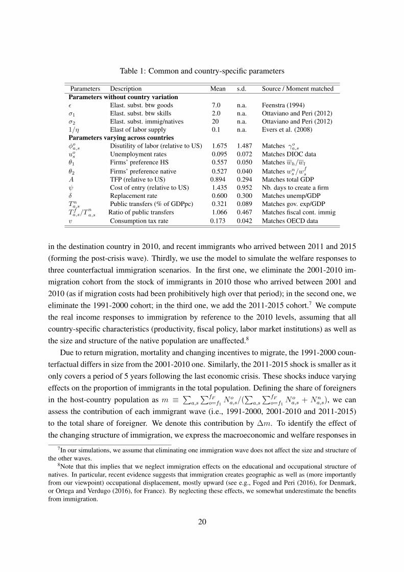
Table 1: Common and country-specific parameters

Parameters Description Mean s.d. Source / Moment matchedParameters without country variationε Elast. subst. btw goods 7.0 n.a. Feenstra (1994)σ1 Elast. subst. btw skills 2.0 n.a. Ottaviano and Peri (2012)σ2 Elast. subst. immig/natives 20 n.a. Ottaviano and Peri (2012)1/η Elast of labor supply 0.1 n.a. Evers et al. (2008)Parameters varying across countriesφoa,s Disutility of labor (relative to US) 1.675 1.487 Matches γoa,suos Unemployment rates 0.095 0.072 Matches DIOC dataθ1 Firms’ preference HS 0.557 0.050 Matches wh/wl

θ2 Firms’ preference native 0.527 0.040 Matches wns /w

fs

A TFP (relative to US) 0.894 0.294 Matches total GDPψ Cost of entry (relative to US) 1.435 0.952 Nb. days to create a firmδ Replacement rate 0.600 0.300 Matches unemp/GDPTna,s Public transfers (% of GDPpc) 0.321 0.089 Matches gov. exp/GDPT fa,s/T

na,s Ratio of public transfers 1.066 0.467 Matches fiscal cont. immig

v Consumption tax rate 0.173 0.042 Matches OECD data

in the destination country in 2010, and recent immigrants who arrived between 2011 and 2015(forming the post-crisis wave). Thirdly, we use the model to simulate the welfare responses tothree counterfactual immigration scenarios. In the first one, we eliminate the 2001-2010 im-migration cohort from the stock of immigrants in 2010 those who arrived between 2001 and2010 (as if migration costs had been prohibitively high over that period); in the second one, weeliminate the 1991-2000 cohort; in the third one, we add the 2011-2015 cohort.7 We computethe real income responses to immigration by reference to the 2010 levels, assuming that allcountry-specific characteristics (productivity, fiscal policy, labor market institutions) as well asthe size and structure of the native population are unaffected.8

Due to return migration, mortality and changing incentives to migrate, the 1991-2000 coun-terfactual differs in size from the 2001-2010 one. Similarly, the 2011-2015 shock is smaller as itonly covers a period of 5 years following the last economic crisis. These shocks induce varyingeffects on the proportion of immigrants in the total population. Defining the share of foreignersin the host-country population as m ≡

∑a,s

∑fFo=f1

N oa,s/(

∑a,s

∑fFo=f1

N oa,s + Nn

a,s), we canassess the contribution of each immigrant wave (i.e., 1991-2000, 2001-2010 and 2011-2015)to the total share of foreigner. We denote this contribution by ∆m. To identify the effect ofthe changing structure of immigration, we express the macroeconomic and welfare responses in

7In our simulations, we assume that eliminating one immigration wave does not affect the size and structure ofthe other waves.

8Note that this implies that we neglect immigration effects on the educational and occupational structure ofnatives. In particular, recent evidence suggests that immigration creates geographic as well as (more importantlyfrom our viewpoint) occupational displacement, mostly upward (see e.g., Foged and Peri (2016), for Denmark,or Ortega and Verdugo (2016), for France). By neglecting these effects, we somewhat underestimate the benefitsfrom immigration.

20

relative terms by dividing all effects by ∆m; we thus report semi-elasticities of macroeconomicvariables and welfare to immigration. For each type of native individual in the year 2010, thesemi-elasticity of real income to immigration can be expressed as:

∆Cna,s/C

na,s

∆m=

(Cna,s

)With Mig

−(Cna,s

)Without Mig

∆m(Cna,s

)Without Mig

. (13)

The relative change in real income is expressed as percentage deviation from the no-migrationcounterfactual (i.e., after eliminating the 1991-2000 or 2001-2010 pre-crisis waves in the firsttwo experiments, or before adding the 2011-2015 post-crisis wave in the third experiment).Hence, a positive deviation implies a welfare gain due to the immigration wave, while a nega-tive deviation implies a welfare loss. The same expression is used when discussing the effecton any extensive macroeconomic variable (in USD). When describing the effect on intensivevariables (i.e., a variable which does depend on the volume of the system, such as the tax rate,the (un)employment rate, the proportion of college graduates, the support ratio, etc.), we simplydivide the numerator of the expression above by ∆m.

The model accounts for four interdependent mechanisms of transmission. Two of themwork through the labor market. Firstly, immigration affects the size and structure of the laborforce. The greater the employment rate of immigrants, the larger the labor supply shock. Thelatter induces responses in nominal wages. The skill structure of immigration determines whowins and who loses among natives. Other things being equal, immigration also induces a wagesurplus for natives (i.e., the wage gains for the winners exceed the wage losses for the losers);the size of this wage surplus is small in this type of model (Borjas, 1995). Secondly, wageresponses affect the participation rates of natives and former immigrants. Thirdly, immigrationaffects the amounts of public revenues and expenditures. If it induces a fiscal gain, immigrationreduces the equilibrium tax rate; otherwise, the tax rate increases. In our experiments, immi-gration usually generates a fiscal gain. Given the transfer profiles by age and by skill group, thefiscal contribution of immigrants increases with their education level and with their employmentrate. Fourthly, immigration increases the total demand for goods and services, which supportsentrepreneurship and the number of varieties available to consumers. Hence, the ideal priceindex decreases. General equilibrium interdependencies result from the fact that responses innominal wages, tax rates and prices affect labor-market participation rates and vice versa. Thereal income of working-age natives is affected by wages, taxes, prices, and labor supply deci-sions. Native retirees, on the other hand, are assumed to receive no labor income, to pay notaxes, and to be affected only through the market size channel (i.e., by the price response toimmigration).

In this section, we first describe the three immigration waves in Section (4.1). We then

21

discuss the macroeconomic effects of immigration in Section (4.2). Section (4.3) describes thewelfare and inequality implications for the native population.

4.1 Immigration cohorts

We describe the effects of the counterfactuals on socio-demographic variables, i.e. on thepopulation size, on the proportion of college graduates in the working age population, h ≡∑

oNoy,h/

∑o,sN

oy,s, and on the support ratio defined as the ratio of working age residents to

population: s ≡∑

o,sNoy,s/

∑o,a,sN

oa,s.

The first counterfactual consists of eliminating immigrants who arrived between 2001 and2010. Data on immigrants by duration of stay, by origin country and by education level areavailable from the DIOC database. The same database can be used to characterize the secondcounterfactual, which consists in eliminating immigrants who arrived between 1991 and 2000.These cohorts are not perfectly comparable: immigrants arrived between 1991 and 2000 areolder and had more opportunities to return to their home country. Hence, the remaining mem-bers of this cohort in the year 2010 can be more or less educated than those of the next cohortfor other reasons than the changing origin mix. This must be kept in mind when comparing thetwo pre-crisis waves.

As for the third counterfactual, data on the 2011-15 inflow by education level are not avail-able. We use the United Nations data and compute the growth rates of dyadic immigrant stocksbetween 2010 and 2015. We apply these growth rates to the stock of working age immigrantsin 2010, and assume that the additional immigrants have the same education level as migrantsfrom the same origin country arrived between 2001 and 2010. Hence, in the third experiment,the effect of immigration on human capital is totally governed by the changing origin mix of themigrant inflows after the crisis. In the Appendix, we show that this method is highly relevant topredict the skill structure of immigration of past immigrant waves. This is because the dyadiceducation structure is very stable across cohorts. This does not fully guarantee that it is identi-cally relevant to predict the structure of the post-crisis wave, but it mitigates concerns about theunavailability of education data for the latter cohort. We also assume that all adult immigrantsfrom these three waves belong to the working age population.

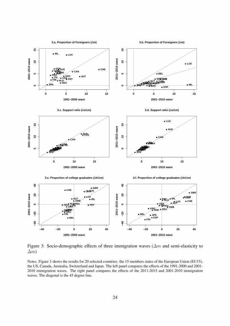
Figure 3 characterizes the socio-demographic effects of these three immigration waves. Theleft panel (Fig 3.a, 3.c and 3.e) compares the effect of the 1991-2000 wave on the horizontalaxis with that of the 2001-2010 wave on the vertical axis. The right panel (Fig 3.b, 3.d and 3.f)compares the effect of the 2001-2010 wave on the horizontal axis with that of the 2011-2015wave on the vertical axis. The 45-degree line allows visualizing which wave dominates.

Figures 3.a and 3.b depict the size of the shocks (∆m). Comparing 1991-2000 with 2001-2010, the average shock sizes equal 3.7 and 5.1 percentage points, respectively. The 2001-

22

2010 wave is larger in 11 countries, including France, Belgium, the United Kingdom, Australiaand Sweden. Changes are drastic in Ireland and Luxembourg. On the contrary, the 1991-2000waves dominates in 8 countries, including Switzerland, Germany, Austria and, to a lesser extent,Canada and the United States. Comparing 2001-2010 with 2011-2015, the average shock sizesequal 5.1 and 1.6 percentage points, respectively (the latter corresponds to a 3.2 p.p. shock overa decade). Overall, Figure 3.b shows that the pre- and post-crisis trends are very similar; thismeans that most observations are close to the 22.5-degree line (i.e., the 5-year shock of 2011-2015 is slightly smaller than half the 10-year shock of 2001-2010). Exceptions are Belgiumand Luxembourg, where the post-crisis migration inflows are larger, and Ireland, where theyare smaller. Remember that in equation (13), we neutralize the size of the shock (∆m) wheninterpreting its welfare implications, in order to highlight the role of the changing structure ofimmigration.

Figures 3.c and 3.d depict the effect on the support ratio (∆s/∆m). Changes in the agestructure govern the fiscal responses to migration. By definition, the semi-elasticity is equalto the ratio of retirees to population and is independent of the size and structure of immigra-tion. Hence, the effect of immigration is greater in countries with older populations (such asGermany, Luxembourg, Austria, Italy or Sweden), and smaller in countries with younger pop-ulations (such as Canada, United States, Australia, Ireland). Hence, immigration increases thesupport ratio everywhere, and particularly in countries where the median age of the nativepopulation is low. This effect does not vary across immigrant cohorts.

As far as the education level is concerned, it varies with the origin mix and with the degreeof self-selection of immigrants. The latter is affected by (unmodelled) dyadic and destinationcharacteristics such as the immigration policy, linguistic proximity, colonial links, geographicdistances, the industry structure, etc. Figures 3.e and 3.f depict the effect of immigration onthe proportion of college graduates (∆h/∆m). Changes in human capital govern the produc-tivity and inequality responses to migration. The two figures show a remarkable persistenceacross immigration waves. Countries where immigration increases human capital include Aus-tralia, Canada and the United Kingdom (i.e., countries conducting quality-selective immigrationpolicies) as well as Luxembourg. On the contrary, immigration reduces human capital in Scan-dinavia, Belgium or Greece. Between 2001 and 2010, immigration increases human capital inSwitzerland and decreases it in Portugal. Figure 3.f shows that most observations are locatedbelow the 45◦ line, implying that, with very few exceptions, the post-crisis immigration waveis relatively less educated than the previous one. This potentially affects their market size andfiscal impacts of immigration.

23

0 5 10 15

05

1015

1991−2000 wave

2001

−201

0 w

ave

AUS

AUT

BEL CANCHE

DEU

DNK

ESP

FIN

FRA

GBR

GRC

IRL

ITA

JPN

LUX

NLDPRT

SWE

USA

3.a. Proportion of Foreigners ( ∆m)

0 5 10 15

05

1015

2001−2010 wave

2011

−201

5 w

ave

AUSAUT

BEL

CANCHE

DEUDNK

ESP

FIN FRA GBR

GRC IRLITAJPN

LUX

NLDPRT

SWE

USA

3.b. Proportion of Foreigners ( ∆m)

5 10 15

510

15

1991−2000 wave

2001

−201

0 w

ave

AUS

AUTBEL

CAN

CHE

DEUDNKESPFINFRAGBR

GRC

IRL

ITAJPN

LUX

NLDPRTSWE

USA

3.c. Support ratio ( ∆s/∆m)

5 10 15

510

15

2001−2010 wave

2011

−201

5 w

ave

AUS

AUTBEL

CAN

CHE

DEUDNKESPFIN

FRAGBRGRC

IRL

ITAJPN

LUX

NLDPRT

SWE

USA

3.d. Support ratio ( ∆s/∆m)

−40 −20 0 20 40

−40

−20

020

40

1991−2000 wave

2001

−201

0 w

ave

AUS

AUT

BEL

CANCHE

DEU

DNKESP

FIN

FRA

GBR

GRC

IRL

ITA

JPN

LUX

NLD PRT

SWE

USA

3.e. Proportion of college graduates ( ∆h/∆m)

−40 −20 0 20 40

−40

−20

020

40

2001−2010 wave

2011

−201

5 w

ave

AUS

AUT

BEL

CANCHE

DEUDNK

ESPFIN

FRA

GBR

GRC

IRL

ITA

JPN

LUXNLDPRT

SWEUSA

3.f. Proportion of college graduates ( ∆h/∆m)

Figure 3: Socio-demographic effects of three immigration waves (∆m and semi-elasticity to∆m)

Notes. Figure 3 shows the results for 20 selected countries: the 15 members states of the European Union (EU15),the US, Canada, Australia, Switzerland and Japan. The left panel compares the effects of the 1991-2000 and 2001-2010 immigration waves. The right panel compares the effects of the 2011-2015 and 2001-2010 immigrationwaves. The diagonal is the 45 degree line.

24

4.2 Macroeconomic effects

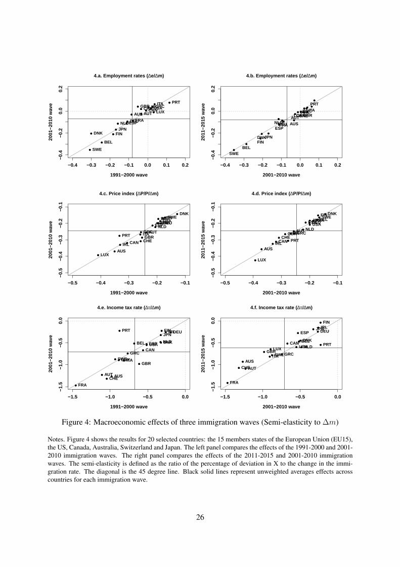
Figure 4 characterizes the macroeconomic effects of the three immigration waves. We focuson the average employment rate, the income tax rate and the average price index. As before,the left panel (Figures 4.a, 4.c and 4.e) compares the effect of the 1991-2000 wave with thatof the 2001-2010 wave. The right panel (Figures 4.b, 4.d and 4.f) compares the effect of the2001-2010 wave with that of the 2011-2015 wave.9

Figures 4.a and 4.b depict the aggregate employment effects of immigration. These effectsmostly depend on the average disutility of labor and induced participation rates of immigrantsand, to a lesser extent, on the endogenous labor-market participation responses of the natives.There are a few countries where immigration increases the average employment rates (e.g.,the poorer countries of Europe). On the contrary, immigration reduces employment rates incountries where immigrants exhibit higher disutility for labor (such as Scandinavian countriesand Belgium). The comparison between cohorts reveals very small differences. In particular,despite its lower level of education, the 2011-2015 wave induces very similar effects comparedto the pre-crisis waves. This is because the correlation between the employment and humancapital levels of immigrants is limited in the data (around 0.5). Hence, employment responsesare very persistent across immigration waves: the degradation of immigrant’s human capitalafter the crisis has small effects on the employment response to immigration, as evidenced fromFigure 4.b.

Figures 4.c and 4.d illustrate the market size effect of immigration. Using a conservativeelasticity of substitution between goods (ε = 7), we obtain non negligible effects on the averageprice index. On average, increasing the immigration share by one percentage point reducesthe average price level by 0.24% in 1991-2000 and in 2001-2010. A similar magnitude of themarket size effect can be observed for the 2011-2015 period. The price elasticity to migrationdepends on changes in human capital and employment rates. Again, these figures show a strongpersistence over immigration waves. Countries where market size effects are large are Australia,Canada, Luxembourg, Ireland. The effect is smaller in Scandinavian countries and Belgium.Remember the market size mechanism is the only channel through which native retirees areeconomically affected by immigration (due to the fixed-benefit fiscal rule). Figure 4.c and 4.dthus depict the impact of immigration on the real income of retirees; this effect is positive in allcountries and across all waves.

The fiscal impact of immigration is described in Figures 4.e and 4.f. Remember that for eachcountry, our model is calibrated to match the estimated fiscal contribution of the total stock ofimmigrants. The latter contribution is the sum of the fiscal costs induced by old immigrants andthe fiscal gains induced by younger immigrants. In our experiments, recent immigration flows

9For detailed country-specific results, please consult Table C2.

25

−0.4 −0.3 −0.2 −0.1 0.0 0.1 0.2

−0.4

−0.2

0.0

0.2

1991−2000 wave

2001

−201

0 w

ave

AUS AUT

BEL

CANCHE

DEU

DNK

ESP

FIN

FRA

GBR GRCIRLITA

JPN

LUX

NLD

PRT

SWE

USA

4.a. Employment rates ( ∆e/∆m)

−0.4 −0.3 −0.2 −0.1 0.0 0.1 0.2

−0.4

−0.2

0.0

0.2

2001−2010 wave

2011

−201

5 w

ave

AUSAUT

BEL

CANCHE

DEU

DNK

ESP

FIN

FRA

GBRGRCIRLITA

JPN

LUX

NLD

PRT

SWE

USA

4.b. Employment rates ( ∆e/∆m)

−0.5 −0.4 −0.3 −0.2 −0.1

−0.5

−0.4

−0.3

−0.2

−0.1

1991−2000 wave

2001

−201

0 w

ave

AUS

AUT

BEL

CAN CHE

DEU

DNK

ESP

FINFRA

GBRGRC

IRL

ITA

JPN

LUX

NLD

PRT

SWEUSA

4.c. Price index ( ∆P/P/∆m)

−0.5 −0.4 −0.3 −0.2 −0.1

−0.5

−0.4

−0.3

−0.2

−0.1

2001−2010 wave

2011

−201

5 w

ave

AUS

AUT

BEL

CANCHE

DEU

DNK

ESP

FINFRA

GBRGRC

IRL

ITA

JPN

LUX

NLD

PRT

SWE

USA

4.d. Price index ( ∆P/P/∆m)

−1.5 −1.0 −0.5 0.0

−1.5

−1.0

−0.5

0.0

1991−2000 wave

2001

−201

0 w

ave

AUSAUT

BEL

CAN

CHE

DEU

DNKESP

FIN

FRA

GBR

GRC

IRL

ITA

JPN

LUX

NLD

PRT

SWE

USA

4.e. Income tax rate ( ∆τ/∆m)

−1.5 −1.0 −0.5 0.0

−1.5

−1.0

−0.5

0.0

2001−2010 wave

2011

−201

5 w

ave

AUS

AUT

BELCAN

CHE

DEU

DNK

ESP

FIN

FRA

GBRGRC

IRL

ITA

JPN

LUX NLD PRT

SWE

USA

4.f. Income tax rate ( ∆τ/∆m)

Figure 4: Macroeconomic effects of three immigration waves (Semi-elasticity to ∆m)

Notes. Figure 4 shows the results for 20 selected countries: the 15 members states of the European Union (EU15),the US, Canada, Australia, Switzerland and Japan. The left panel compares the effects of the 1991-2000 and 2001-2010 immigration waves. The right panel compares the effects of the 2011-2015 and 2001-2010 immigrationwaves. The semi-elasticity is defined as the ratio of the percentage of deviation in X to the change in the immi-gration rate. The diagonal is the 45 degree line. Black solid lines represent unweighted averages effects acrosscountries for each immigration wave.

26

make the population younger. Although immigrants receive higher transfers than natives shar-ing similar characteristics, young immigrants generate a positive contribution to public finances.On average, increasing the immigration share by one percentage point reduces the income taxrate by 0.67 percentage point in 1991-2000, by 0.71 percentage point in 2001-2010, and by 0.62percentage point in 2011-2015. The fiscal impact is strongly persistent across waves; its sizeis governed by fiscal policy and by the age structure of the population. Countries exhibitinglarge fiscal gains are France, Switzerland and Austria (i.e., countries where population aginghas reached an advanced stage or where immigrants receive relatively less transfers). Countrieswhere fiscal gains are consistently smaller are Canada, Germany, the United States (i.e., coun-tries where the population is younger or where immigrants receive relatively more transfers). Inthe majority of countries, the decrease in the average education level of post-crisis immigrantsresults in smaller fiscal gains for natives.

4.3 Welfare and inequality effects

We now aggregate the transmission channels and compute the welfare implications of immi-gration for the natives. As stated above, we use the net-of-tax, real income level as a proxyfor utility. Figure 5 gives the effect on the average real income of working age natives, and theeffect on the real income ratio between young college-educated natives and the less educated.The latter inequality response is essentially governed by the wage effect of immigration: theincome ratio increases if immigrants are less educated than working age natives, and decreasesotherwise. The wage effect is slightly amplified by changes in labor market participation rates.On the contrary, these labor market responses have limited effects on the average real incomeof natives because the immigration wage surplus per se is small (Borjas, 1995). Hence, the av-erage income response is mostly governed by the fiscal and market size effects of immigration,which affect all working age natives with the same intensity. The left panel (Figures 5.a and5.c) compares the effect of the 1991-2000 wave on the horizontal axis with that of the 2001-2010 wave on the vertical axis. The right panel (Figures 5.b and 5.d) compares the effect of the2001-2010 wave on the horizontal axis with that of the 2011-2015 wave on the vertical axis.

Figures 5.a and 5.b show that immigration always increases the real income of workingage natives. In addition, cross-country disparities in the average welfare gain are stronglypersistent across immigration waves. The largest immigration gains are obtained in Australia,Austria, France, Luxembourg, Switzerland and the United Kingdom. The smallest gains areobserved in Scandinavian countries, Germany, Belgium, Spain and the United States. Thelatter set of countries exhibit smaller fiscal and market size gains from immigration. The 2001-2010 immigration wave induces very similar effects as the 1991-2000 one, although the gainincreases for Swiss and British natives, and decreases for the Portuguese. On the contrary,

27

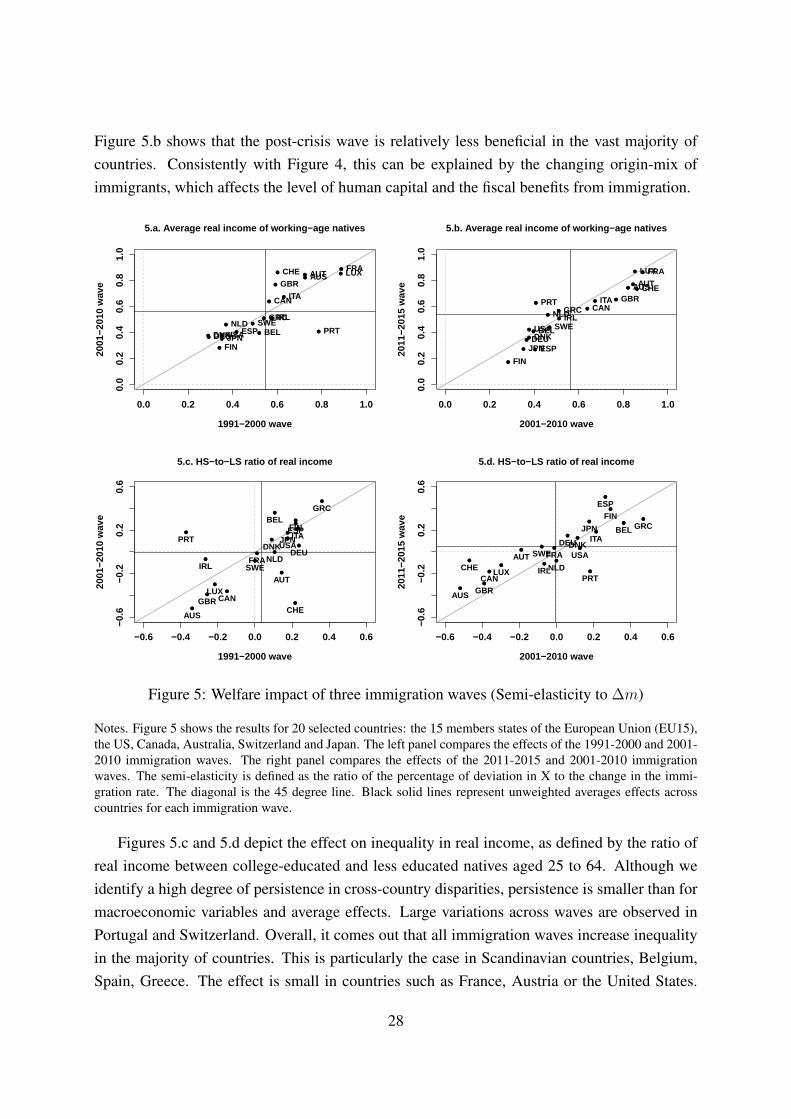
Figure 5.b shows that the post-crisis wave is relatively less beneficial in the vast majority ofcountries. Consistently with Figure 4, this can be explained by the changing origin-mix ofimmigrants, which affects the level of human capital and the fiscal benefits from immigration.

0.0 0.2 0.4 0.6 0.8 1.0

0.0

0.2

0.4

0.6

0.8

1.0

1991−2000 wave

2001

−201

0 w

ave

AUSAUT

BEL

CAN

CHE

DEUDNK ESP

FIN

FRA

GBR

GRCIRL

ITA

JPN

LUX

NLDPRT

SWEUSA

5.a. Average real income of working−age natives

0.0 0.2 0.4 0.6 0.8 1.0

0.0

0.2

0.4

0.6

0.8

1.0

2001−2010 wave

2011

−201

5 w

ave AUSAUT

BEL

CAN

CHE

DEUDNKESP

FIN

FRA

GBRGRCIRL

ITA

JPN

LUX

NLDPRT

SWEUSA

5.b. Average real income of working−age natives

−0.6 −0.4 −0.2 0.0 0.2 0.4 0.6

−0.6

−0.2

0.2

0.6

1991−2000 wave

2001

−201

0 w

ave

AUS

AUT

BEL

CANCHE

DEUDNK

ESPFIN

FRA

GBR

GRC

IRL

ITAJPN

LUX

NLD

PRT

SWE

USA

5.c. HS−to−LS ratio of real income

−0.6 −0.4 −0.2 0.0 0.2 0.4 0.6

−0.6

−0.2

0.2

0.6

2001−2010 wave

2011

−201

5 w

ave

AUS

AUT

BEL

CANCHE

DEUDNK

ESP

FIN

FRA

GBR

GRC

IRL

ITAJPN

LUX NLDPRT

SWE USA

5.d. HS−to−LS ratio of real income

Figure 5: Welfare impact of three immigration waves (Semi-elasticity to ∆m)

Notes. Figure 5 shows the results for 20 selected countries: the 15 members states of the European Union (EU15),the US, Canada, Australia, Switzerland and Japan. The left panel compares the effects of the 1991-2000 and 2001-2010 immigration waves. The right panel compares the effects of the 2011-2015 and 2001-2010 immigrationwaves. The semi-elasticity is defined as the ratio of the percentage of deviation in X to the change in the immi-gration rate. The diagonal is the 45 degree line. Black solid lines represent unweighted averages effects acrosscountries for each immigration wave.

Figures 5.c and 5.d depict the effect on inequality in real income, as defined by the ratio ofreal income between college-educated and less educated natives aged 25 to 64. Although weidentify a high degree of persistence in cross-country disparities, persistence is smaller than formacroeconomic variables and average effects. Large variations across waves are observed inPortugal and Switzerland. Overall, it comes out that all immigration waves increase inequalityin the majority of countries. This is particularly the case in Scandinavian countries, Belgium,Spain, Greece. The effect is small in countries such as France, Austria or the United States.

28

Immigration decreases inequality in countries where migrants are positively selected such asLuxembourg, Australia, Canada and the United Kingdom. This being said, the impact on thereal income of low-skilled natives is almost always positive, as the fiscal and market size effectsdominate labor market effects. The only exceptions are Spain, Japan and Greece after the 2011-2015 wave, where the semi-elasticity of income to migration is negative but virtually nil (the lossis smaller than 0.1%). Figure 5.d shows that the post-crisis cohort induces more inegalitarian(or less egalitarian) effects than the pre-crisis cohort in two thirds of the countries. The oppositeeffect is found in the rest of the sample.

Overall, the key findings of our analysis are that (i) the last three waves of immigrationhave not deteriorated the real income of the native population, (ii) that the distribution of thegains vary across countries and across skill groups as a function of the structure of immigration,(iii) that these redistributive effects are strongly persistent over time, and (iv) that the post-crisisimmigration waves is less beneficial for natives than the previous ones, and more inegalitarian inthe majority of countries (keeping in mind that its skill structure is not directly observable, but isestimated). In the Appendix, we show that the results of the benchmark model are highly robustto the choice of parameters, to the inclusion of technological externalities, and to alternativefiscal rules.

5 Concluding remarks

Despite large changes in the number and in the origin-mix of immigrants, little is known aboutthe evolution of their welfare impact on the native populations in the OECD member states.This paper compares the welfare implications of two pre-crisis immigration waves (1991–2000and 2001–2010) to those of the post-crisis wave (2011–2015). Our analysis relies on a generalequilibrium model that accounts for the main channels of transmission of immigration shocks– the employment and wage effects, the fiscal effect, and the market size effect – and for theinteractions between them. Focusing on 20 selected OECD member states, we find that thethree waves induce positive effects on the real income of natives, although the size of thesegains varies across countries and across skill groups. For example, we estimate that increasingthe immigrant share in the total population by one percentage point raises the average incomeof natives by 0.5% in the OECD member states. However, this effect varies between 0.3% inFinland and 0.9% in Luxembourg. As far as income inequality is concerned, the same inflowof immigrants increases the ratio of real income between college graduates and the less edu-cated by 0.5% in Greece, and decreases it by 0.5% in Australia. These average welfare gainand inequality effects are strongly persistent across immigration waves. In relative terms, thepost-crisis wave induces smaller welfare gains compared to the previous ones (on average, -0.02% for each percentage point of immigration). This is due to the changing origin-mix of

29

immigrants, which translates into lower levels of human capital and smaller fiscal gains. Thisoverall result applies to all OECD countries and to all categories of native citizens. However,differences across cohorts explain a tiny fraction of the highly persistent, cross-country hetero-geneity in the economic benefits from immigration. This heterogeneity is presumably governedby enduring destination characteristics such as the immigration policy, the wage structure, orthe industry structure. This implies that the economic consequences of the changing origin mixof immigrants should not be overestimated.

ReferencesAbramitzky, R., Boustan, J., and Eriksson, K. (2012). Europe’s tired, poor, huddled masses:

Self-selection and economic outcomes in the age of mass migration. American EconomicReview, 102(5):1832–1856.

Alesina, A., Harnoss, J., and Rapoport, H. (2016). Birthplace diversity and economic prosperity.Journal of Economic Growth, pages 1–32.

Ambrosini, J. and Peri, G. (2012). The determinants and the selection of mexico-us migrants.World Economy, 35(2):111–151.

Anderson, J. E., Larch, M., and Yotov, Y. V. (2016). Trade liberalization, growth, and fdi: Astructural estimation framework.

Arslan, C., Dumont, J.-C., Kone, Z., Moullan, Y., Özden, c., Parsons, C., and Xenogiani, T.(2015). A new profile of migrants in the aftermath of the recent economic crisis. OECDSocial, Employment and Migration Working Papers, (160).

Aubry, A., Burzynski, M., and Docquier, F. (2016). The welfare impact of global migration inoecd countries. Journal of International Economics, 101:1–21.

Bahar, D. and Rapoport, H. (2017). Migration, knowledge diffusion and the comparative ad-vantage of nations. Economic Journal, forthcoming.

Battisti, M., Felbermayr, G., Peri, G., and Poutvaara, P. (2017). Immigration, search and redis-tribution: A quantitative assessment of native welfare. Journal of the European EconomicAssociation.

Borjas, G. J. (1993). Immigration policy, national origin, and immigrant skills: A comparison ofcanada and the united states. In: Small Differences that Matter: Labor Markets and IncomeMaintenance in Canada and the United States, D. Card and R.B. Freeman (eds.), Universityof Chicago Press.

Borjas, G. J. (1995). The economic benefits from immigration. Journal of Economic Perspec-tives, 9(2):3–22.

30

Borjas, G. J. and Trejo, S. J. (1993). National origin and immigrant welfare recipiency. Journalof Public Economics, 50(3):325–344.

Büchel, F. and Frick, J. R. (2005). Immigrants economic performance across Europe-doesimmigration policy matter? Population Research and Policy Review, 24(2):175–212.

Card, D. (2009). Immigration and inequality. American Economic Review, 99(2):1–21.

Chiquiar, D. and Hanson, G. (2005). International migration, self-selection and the distribu-tion of wages: Evidence from mexico and the united states. Journal of Political Economy,113(2):239–281.

de la Croix, D. and Docquier, F. (2012). Do brain drain and poverty result from coordinationfailures? Journal of Economic Growth, 17(1):1–26.

di Giovanni, J., Levchenko, A. A., and Ortega, F. (2015). A global view of cross-border migra-tion. Journal of the European Economic Association, 13(1):168–202.

Docquier, F., Ozden, Ç., and Peri, G. (2014). The labour market effects of immigration andemigration in oecd countries. Economic Journal, 124(579):1106–1145.

Docquier, F., Turati, R., Valette, J., and Vasilakis, C. (2016). Multiculturalism and growth:Skill-specific evidence from the post-world war II period. IRES Discussion Papers, (28).

Evers, M. and De Mooij, R Van Vuuren, D. (2008). The wage elasticity of labour supply: asynthesis of empirical estimates. De Economist, 156(1):25–43.

Facchini, G. and Mayda, A. M. (2009). Does the welfare state affect individual attitudes towardimmigrants? evidence across countries. The Review of Economics and Statistics, 91(2):295–314.

Feenstra, R. C. (1994). New product varieties and the measurement of international prices.American Economic Review, 84(1):157–177.

Felbermayr, G. J., Jung, B., and Toubal, F. (2010). Ethnic networks, information, and interna-tional trade: Revisiting the evidence. Annals of Economics and Statistics/Annales dâAZE-conomie et de Statistique, pages 41–70.

Felbermayr, G. J. and Toubal, F. (2012). Revisiting the trade-migration nexus: Evidence fromnew oecd data. World Development, 40(5):928–937.

Feyrer, J. (2009). Trade and income–exploiting time series in geography.

Foged, M. and Peri, G. (2016). Immigrants’ effect on native workers: New analysis on longitu-dinal data. American Economic Journal: Applied Economics, 8(2):1–34.

Iranzo, S. and Peri, G. (2009). Migration and trade: Theory with an application to the eastern–western european integration. Journal of International Economics, 79(1):1–19.

31

Javorcik, B. S., Özden, Ç., Spatareanu, M., and Neagu, C. (2011). Migrant networks and foreigndirect investment. Journal of Development Economics, 94(2):231–241.

Kaestner, R. and Malamud, O. (2014). Self-selection and international migration: New evidencefrom mexico. Review of Economics and Statistics, 96(1):78–91.

Kerr, W. R. (2017). Heterogeneous technology diffusion and ricardian trade patterns. WorldBank Economic Review.

Krugman, P. (1980). Scale economies, product differentiation, and the pattern of trade. Ameri-can Economic Review, pages 950–959.

Kugler, M. and Rapoport, H. (2007). International labor and capital flows: Complements orsubstitutes? Economics Letters, 94(2):155–162.

McKenzie, D. and Rapoport, H. (2010). Self-selection patterns in mexico-us migration: the roleof migration networks. Review of Economics and Statistics, 92(4):811–821.

Moraga, J. F.-H. (2011). New evidence on emigrant selection. Review of Economics andStatistics, 93(1):72–96.

Moretti, E. (2004a). Estimating the social return to higher education: evidence from longitudi-nal and repeated cross-sectional data. Journal of Econometrics, 121(1):175–212.

Moretti, E. (2004b). Workers’ education, spillovers, and productivity: evidence from plant-levelproduction functions. American Economic Review, 94(3):656–690.

OECD (2013). The fiscal impact of immigration in oecd countries. International MigrationOutlook.

Ortega, F. and Peri, G. (2014). Openness and income: The roles of trade and migration. Journalof International Economics, 92(2):231–251.

Ortega, J. and Verdugo, G. (2016). Moving up or down? immigration and the selection ofnatives across occupations and locations. Working Paper, UniversitÃl’ Paris 1 PanthÃl’on-Sorbonne.

Ottaviano, G. I. and Peri, G. (2012). Rethinking the effect of immigration on wages. Journal ofthe European Economic Association, 10(1):152–197.

Özden, Ç., Parsons, C. R., Schiff, M., and Walmsley, T. L. (2011). Where on earth is every-body? the evolution of global bilateral migration 1960–2000. World Bank Economic Review,25(1):12–56.

Parsons, C. R. and Vézina, P.-L. (2017). Migrant networks and trade: The vietnamese boatpeople as a natural experiment. Economic Journal, forthcoming.

Steingress, W. (2015). The causal impact of migration on us trade: Evidence from a naturalexperiment. IZA Working Paper, (9058).

32

Storesletten, K. (2000). Sustaining fiscal policy through immigration. Journal of PoliticalEconomy, 108(2):300–323.

United Nations (2014). United nations global migration database (ungmd). United NationsDepartment of Economic and Social Affairs Population Division.

33

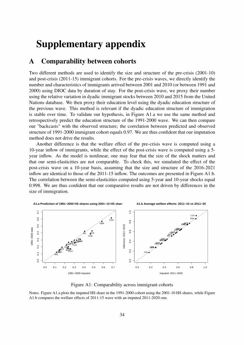
Supplementary appendixA Comparability between cohortsTwo different methods are used to identify the size and structure of the pre-crisis (2001-10)and post-crisis (2011-15) immigrant cohorts. For the pre-crisis waves, we directly identify thenumber and characteristics of immigrants arrived between 2001 and 2010 (or between 1991 and2000) using DIOC data by duration of stay. For the post-crisis wave, we proxy their numberusing the relative variation in dyadic immigrant stocks between 2010 and 2015 from the UnitedNations database. We then proxy their education level using the dyadic education structure ofthe previous wave. This method is relevant if the dyadic education structure of immigrationis stable over time. To validate our hypothesis, in Figure A1.a we use the same method andretrospectively predict the education structure of the 1991-2000 wave. We can then compareour "backcasts" with the observed structure; the correlation between predicted and observedstructure of 1991-2000 immigrant cohort equals 0.97. We are thus confident that our imputationmethod does not drive the results.

Another difference is that the welfare effect of the pre-crisis wave is computed using a10-year inflow of immigrants, while the effect of the post-crisis wave is computed using a 5-year inflow. As the model is nonlinear, one may fear that the size of the shock matters andthat our semi-elasticities are not comparable. To check this, we simulated the effect of thepost-crisis wave on a 10-year basis, assuming that the size and structure of the 2016-2021inflow are identical to those of the 2011-15 inflow. The outcomes are presented in Figure A1.b.The correlation between the semi-elasticities computed using 5-year and 10-year shocks equal0.998. We are thus confident that our comparative results are not driven by differences in thesize of immigration.

0.0 0.1 0.2 0.3 0.4 0.5 0.6 0.7

0.0

0.1

0.2

0.3

0.4

0.5

0.6

0.7

1991−2000 imputed

1991

−20

00 d

ata

AUS

AUT

BEL

CAN

CHE

DEUDNK

ESPFIN

FRA

GBR

GRC

IRL

ITA

JPNLUXNLD

PRT

SWEUSA

A1.a Prediction of 1991−2000 HS shares using 2001−10 HS shares

0.0 0.2 0.4 0.6 0.8 1.0

0.0

0.2

0.4

0.6

0.8

1.0

imputed: 2011−2020

refe

renc

e: 2

011−

2015

AUSAUT

BEL

CAN

CHE

DEUDNK

ESP

FIN

FRA

GBR

GRCIRL

ITA

JPN

LUX

NLD

PRT

SWEUSA

A1.b Average welfare effects: 2011−15 vs 2011−20

Figure A1: Comparability across immigrant cohorts

Notes. Figure A1.a plots the imputed HS share in the 1991-2000 cohort using the 2001-10 HS shares, while FigureA1.b compares the welfare effects of 2011-15 wave with an imputed 2011-2020 one.

34

B Robustness checksIn this section, we investigate whether the conclusions of the benchmark analysis are robust tothe choice of parameters, to the inclusion of technological externalities, to the fiscal rule used tobalanced the government budget constraint, and to the characteristics of immigrants. Focusingon the effect of the 2001-2010 wave, we assess the sensitivity of its impact on the average levelof real income and on income inequality. Figure B2 depicts the results obtained under ninevariants of the benchmark model.

Sensitivity to elasticities. In Figures B2.a and B2.b, we consider alternative levels for threeelasticities, namely for the elasticity of substitution between goods in the utility function (ε = 4instead of 7), for the elasticity of substitution between immigrant and native workers in produc-tion (σ2 = 50 instead of 20), and for the inverse of the elasticity of labor supply to labor income(η = 5 instead of 10).10 For these three variants, we recalibrate the TFP (A) and the disutilityof labor (φ) to match observed GDP levels and participation rates in 2010, and simulate theno-migration counterfactual.

Figure B2.a shows that the average welfare impact of immigration is one and a half timesgreater when the elasticity of substitution between goods equals 4, and 1.2 times greater whenlabor market participation rates are more elastic to labor income. Increasing the elasticity ofsubstitution between immigrant and native workers to 50 has a minor impact on our results. Inall variants, the correlation with the benchmark results exceeds 0.99. As far as the inequalityimpact is concerned, results are almost independent on the choice of elasticity (see Figure B2.b).Hence, the welfare effects depicted in Figure 5 are highly robust to the choice of elasticities.

Sensitivity to externalities. In Figures B2.c and B2.d, we account for three TFP externalities.The first one is a schooling externality; it assumes that the elasticity of TFP to the proportion ofcollege graduates in the labor force is equal to 0.3, in line with de la Croix and Docquier (2012)or Aubry et al. (2016). The second one is a diversity externality; it assumes that the semi-elasticity of TFP to birthplace diversity is equal to 0.2, as in Alesina et al. (2016) or Ortega andPeri (2014). The third one is a diaspora externality which captures the effect of migration ontrade and FDI, and the resulting effect of trade and FDI on TFP. Although our model does notaccount for trade and FDI, we directly model the TFP externality due to the presence of migrantdiasporas. A first strand of literature has identified a causal impact of migration on trade andFDI, with respective elasticities of 0.1 and 0.2.11 Another strand has identified a causal effectof trade and FDI on TFP, with respective elasticities of 0.3 and 0.01 (see Anderson et al., 2016;Feyrer, 2009). Combining these findings gives an elasticity of TFP to migration of 0.035. For

10An additional robustness check has been run to validate our assumption about identical elasticities of substi-tution between natives and migrants in both of the skill groups considered. Following Ottaviano and Peri (2012),we set the above-mentioned parameter to 14 in the group of high-school dropouts. We find that the welfare effectfor the low-skilled immigrants is more pronounced (the difference with the benchmark is below 1.5 p.p.), whilethe rest of worker types are unaffected.

11On migration and trade, see for example Iranzo and Peri (2009), Felbermayr et al. (2010), Felbermayr andToubal (2012) and, for studies exploiting natural experiments, Parsons and Vézina (2017) and Steingress (2015).On migration and FDI, see Kugler and Rapoport (2007) and Javorcik et al. (2011).

35

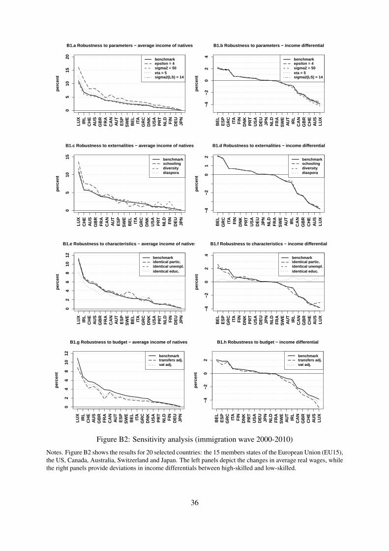
05

1015

20

perc

ent

B1.a Robustness to parameters − average income of natives

LUX

IRL

CH

EA

US

GB

RF

RA

CA

NA

UT

ES

PS

WE

BE

LIT

AG

RC

DN

KU

SA

PR

TN

LD FIN

DE

UJP

N

benchmarkepsilon = 4sigma2 = 50eta = 5sigma2(LS) = 14

−4−2

02

4

perc

ent

B1.b Robustness to parameters − income differential

BE

LE

SP

GR

CIT

AF

IND

NK

PR

TU

SA

DE

UJP

NN

LDF

RA

SW

EA

UT

IRL

CA

NG

BR

CH

EA

US

LUX

benchmarkepsilon = 4sigma2 = 50eta = 5sigma2(LS) = 14

05

1015

perc

ent

B1.c Robustness to externalities − average income of natives

LUX

CH

EA

US

GB

RF

RA

CA

NA

UT

ES

PS

WE

BE

LIT

AG

RC

DN

KU

SA

PR

TN

LD FIN

DE

UJP

N

benchmarkschoolingdiversitydiaspora

−4−2

01

2

perc

ent

B1.d Robustness to externalities − income differential

BE

LG

RC

ITA

FIN

DN

KP

RT

US

AD

EU

JPN

NLD

FR

AS

WE

AU

TIR

LC

AN

GB

RC

HE

AU

SLU

X

benchmarkschoolingdiversitydiaspora

02

46

810

12

perc

ent

B1.e Robustness to characteristics − average income of natives

LUX

IRL

CH

EA

US

GB

RF

RA

CA

NA

UT

ES

PS

WE

BE

LIT

AG

RC

DN

KU

SA

PR

TN

LD FIN

DE

UJP

N

benchmarkidentical partic.identical unempl.identical educ.

−4−2

02

4

perc

ent

B1.f Robustness to characteristics − income differential

BE

LE

SP

GR

CIT

AF

IND

NK

PR

TU

SA

DE

UJP

NN

LDF

RA

SW

EA

UT

IRL

CA

NG

BR

CH

EA

US

LUX

benchmarkidentical partic.identical unempl.identical educ.

02

46

810

12

perc

ent

B1.g Robustness to budget − average income of natives

LUX

IRL

CH

EA

US

GB

RF

RA

CA

NA

UT

ES

PS

WE

BE

LIT

AG

RC

DN

KU

SA

PR

TN

LD FIN

DE

UJP

N

benchmarktransfers adj.vat adj.

−4−2

02

perc

ent

B1.h Robustness to budget − income differential

BE

LE

SP

GR

CIT

AF

IND

NK

PR

TU

SA

DE

UJP

NN

LDF

RA

SW

EA

UT

IRL

CA

NG

BR

CH

EA

US

LUX

benchmarktransfers adj.vat adj.

Figure B2: Sensitivity analysis (immigration wave 2000-2010)

Notes. Figure B2 shows the results for 20 selected countries: the 15 members states of the European Union (EU15),the US, Canada, Australia, Switzerland and Japan. The left panels depict the changes in average real wages, whilethe right panels provide deviations in income differentials between high-skilled and low-skilled.

36

these three variants, we calibrate the scale factors of the TFP function to match the GDP levelsin 2010, and simulate the no-migration counterfactual.

Figure 6.c shows that the schooling externality significantly increases the gain from immi-gration in countries attracting college-educated migrants (such as Australia, Luxembourg, theUnited Kingdom and Switzerland) while it reduces the gain in Spain, Belgium and Greece.Birthplace diversity quantitatively matters only in newer immigration countries such as Ireland,Portugal and Finland. At the estimated elasticity levels, the diaspora externality has negligibleeffects on the results. Results for inequality are almost independent on the inclusion of exter-nalities (see Figure B2.d). Again, the welfare effects depicted on Figure 5 are highly robust toTFP externalities.

Sensitivity to immigrants’ characteristics. In Figures B2.e and B2.f, we consider three al-ternative distributions of characteristics of immigrant workers. We first assume that all im-migrants have the same disutility of labor as natives (same φ’s). We then assume they haveidentical unemployment rate as natives (same u’s). Finally, we assume identical skill structuresfor the immigrant and native populations (same h’s). For these three variants, we simulate thenew hypothetical benchmark for 2010 (keeping other parameters constant), and simulate theno-migration counterfactuals.

Figure B2.e shows that the average welfare gain from immigration is highly robust to labormarket characteristics of immigrants. Imposing the same disutility of labor (governing partic-ipation rates) or the same unemployment rate as native workers marginally affects the results,with the exception of Scandinavian countries and Belgium. Inequality responses are also robustto labor market characteristics. This is in line with the fact that changes in employment ratesin the post-crisis period hardly affected the welfare impact of immigration. On the contrary,equalizing immigrants’ and natives’ levels of schooling reduces the gains from immigrationin "selective" countries (Figure B2.e), and neutralizes the inequality responses to immigration(Figure B2.f). This confirms that the level of human capital of immigrants affects the macroe-conomic and welfare responses to immigration; the degradation of immigrant’s human capitalafter the crisis is responsible for smaller welfare gains.

Sensitivity to the fiscal rule. In our benchmark model, we assume that the income tax rateadjusts to balance the government budget constraint. We consider two alternative fiscal rules,using the consumption tax rate or the amount of public transfers as the adjustment variable.Figures B2.g and B2.h show that the average welfare gain from immigration is highly robustto the fiscal rule. Slightly smaller gains are obtained when public transfers or consumption taxrates are used to adjust the budget. This is because the fiscal gain is now shared between youngand old natives.

37

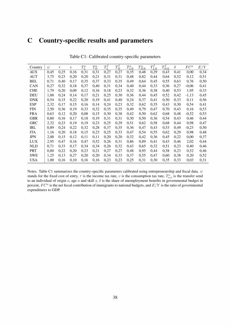
C Country-specific results and parameters

Table C1: Calibrated country-specific parameters

Country ψ τ v TnL Tn

H T fL T f

H TnLR Tn

HR T fLR T f

HR δ FCn E/YAUS 0,45 0,25 0,16 0,31 0,31 0,27 0,27 0,35 0,48 0,29 0,43 0,41 0,00 0,34AUT 3,75 0,23 0,20 0,20 0,21 0,31 0,31 0,48 0,82 0,44 0,64 0,52 0,12 0,51BEL 0,71 0,40 0,17 0,35 0,37 0,33 0,35 0,49 0,64 0,45 0,55 0,63 0,76 0,50CAN 0,27 0,32 0,18 0,37 0,40 0,31 0,34 0,40 0,44 0,33 0,36 0,27 -0,06 0,41CHE 1,79 0,20 0,09 0,12 0,16 0,18 0,23 0,32 0,36 0,38 0,40 0,53 1,95 0,33DEU 1,88 0,24 0,14 0,17 0,21 0,25 0,30 0,36 0,44 0,45 0,52 0,42 -1,13 0,45DNK 0,54 0,15 0,22 0,20 0,19 0,41 0,40 0,24 0,37 0,41 0,50 0,33 0,11 0,56ESP 2,32 0,17 0,15 0,16 0,14 0,24 0,23 0,32 0,62 0,35 0,43 0,30 0,54 0,41FIN 2,50 0,36 0,19 0,33 0,32 0,35 0,35 0,49 0,79 0,47 0,70 0,43 0,16 0,53FRA 0,63 0,12 0,20 0,08 0,15 0,30 0,38 0,42 0,50 0,62 0,68 0,48 -0,52 0,53GBR 0,80 0,16 0,17 0,18 0,19 0,31 0,31 0,30 0,50 0,36 0,54 0,43 0,46 0,44GRC 2,32 0,23 0,19 0,19 0,23 0,25 0,29 0,51 0,62 0,58 0,68 0,44 0,98 0,47IRL 0,89 0,24 0,22 0,32 0,28 0,37 0,35 0,36 0,47 0,43 0,53 0,49 -0,23 0,50ITA 1,16 0,20 0,18 0,15 0,23 0,25 0,33 0,47 0,54 0,55 0,62 0,29 0,98 0,48JPN 2,00 0,15 0,12 0,11 0,11 0,20 0,20 0,32 0,42 0,36 0,45 0,22 0,00 0,37LUX 2,95 0,47 0,16 0,47 0,52 0,26 0,31 0,86 0,89 0,41 0,43 0,46 2,02 0,44NLD 0,71 0,33 0,17 0,34 0,34 0,26 0,32 0,43 0,65 0,32 0,51 0,23 0,40 0,46PRT 0,80 0,22 0,20 0,23 0,21 0,27 0,27 0,48 0,95 0,44 0,58 0,23 0,52 0,46SWE 1,25 0,13 0,27 0,20 0,20 0,34 0,33 0,37 0,55 0,47 0,60 0,38 0,20 0,52USA 1,00 0,16 0,10 0,16 0,16 0,23 0,23 0,25 0,31 0,30 0,35 0,33 0,03 0,31

Notes. Table C1 summarizes the country-specific parameters calibrated using entrepreneurship and fiscal data. ψstands for the fixed cost of entry, τ is the income tax rate, v is the consumption tax rate, T o

s,a is the transfer sendto an individual of origin o, age a and skill s, δ is the share of unemployment benefits in governmental budget inpercent, FCn is the net fiscal contribution of immigrants to national budgets, andE/Y is the ratio of governmentalexpenditures to GDP.

38

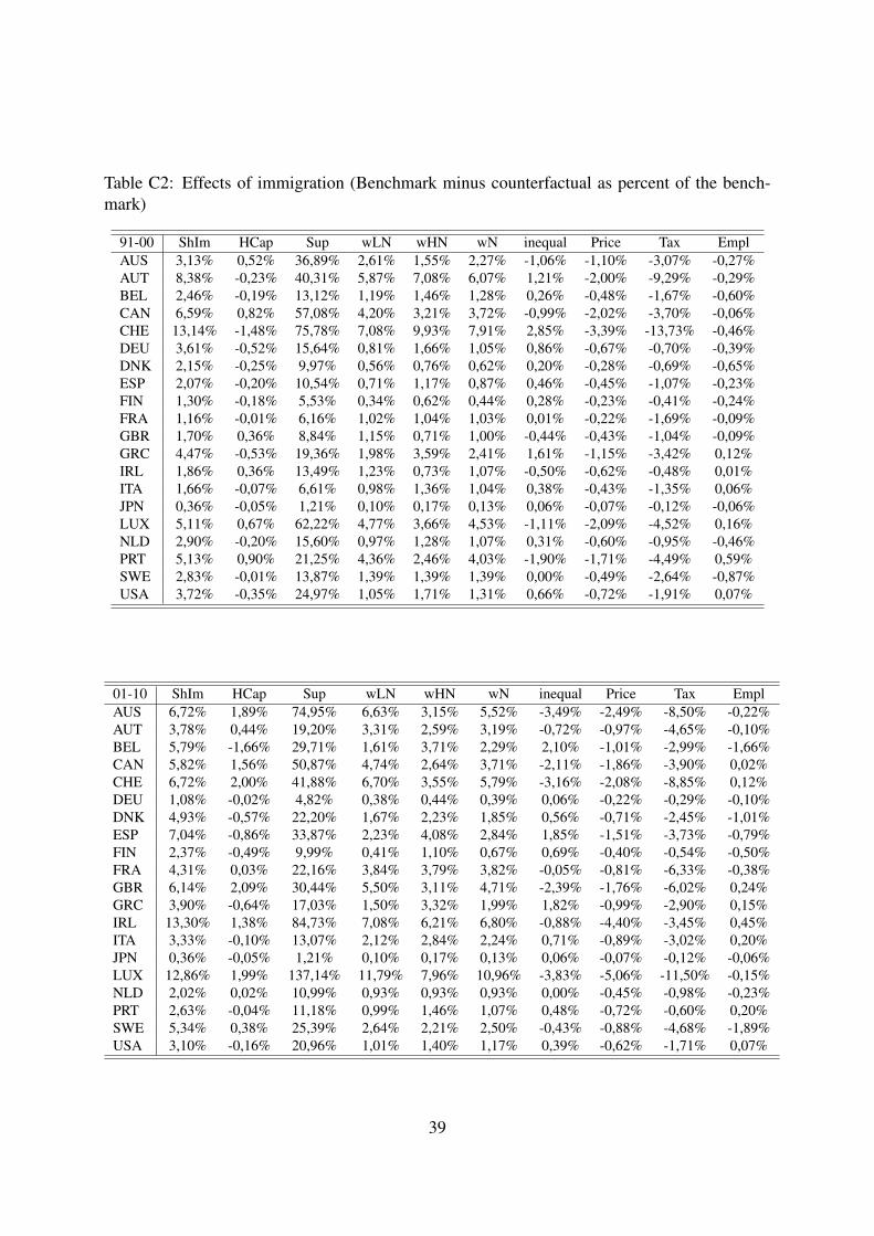
Table C2: Effects of immigration (Benchmark minus counterfactual as percent of the bench-mark)

91-00 ShIm HCap Sup wLN wHN wN inequal Price Tax EmplAUS 3,13% 0,52% 36,89% 2,61% 1,55% 2,27% -1,06% -1,10% -3,07% -0,27%AUT 8,38% -0,23% 40,31% 5,87% 7,08% 6,07% 1,21% -2,00% -9,29% -0,29%BEL 2,46% -0,19% 13,12% 1,19% 1,46% 1,28% 0,26% -0,48% -1,67% -0,60%CAN 6,59% 0,82% 57,08% 4,20% 3,21% 3,72% -0,99% -2,02% -3,70% -0,06%CHE 13,14% -1,48% 75,78% 7,08% 9,93% 7,91% 2,85% -3,39% -13,73% -0,46%DEU 3,61% -0,52% 15,64% 0,81% 1,66% 1,05% 0,86% -0,67% -0,70% -0,39%DNK 2,15% -0,25% 9,97% 0,56% 0,76% 0,62% 0,20% -0,28% -0,69% -0,65%ESP 2,07% -0,20% 10,54% 0,71% 1,17% 0,87% 0,46% -0,45% -1,07% -0,23%FIN 1,30% -0,18% 5,53% 0,34% 0,62% 0,44% 0,28% -0,23% -0,41% -0,24%FRA 1,16% -0,01% 6,16% 1,02% 1,04% 1,03% 0,01% -0,22% -1,69% -0,09%GBR 1,70% 0,36% 8,84% 1,15% 0,71% 1,00% -0,44% -0,43% -1,04% -0,09%GRC 4,47% -0,53% 19,36% 1,98% 3,59% 2,41% 1,61% -1,15% -3,42% 0,12%IRL 1,86% 0,36% 13,49% 1,23% 0,73% 1,07% -0,50% -0,62% -0,48% 0,01%ITA 1,66% -0,07% 6,61% 0,98% 1,36% 1,04% 0,38% -0,43% -1,35% 0,06%JPN 0,36% -0,05% 1,21% 0,10% 0,17% 0,13% 0,06% -0,07% -0,12% -0,06%LUX 5,11% 0,67% 62,22% 4,77% 3,66% 4,53% -1,11% -2,09% -4,52% 0,16%NLD 2,90% -0,20% 15,60% 0,97% 1,28% 1,07% 0,31% -0,60% -0,95% -0,46%PRT 5,13% 0,90% 21,25% 4,36% 2,46% 4,03% -1,90% -1,71% -4,49% 0,59%SWE 2,83% -0,01% 13,87% 1,39% 1,39% 1,39% 0,00% -0,49% -2,64% -0,87%USA 3,72% -0,35% 24,97% 1,05% 1,71% 1,31% 0,66% -0,72% -1,91% 0,07%

01-10 ShIm HCap Sup wLN wHN wN inequal Price Tax EmplAUS 6,72% 1,89% 74,95% 6,63% 3,15% 5,52% -3,49% -2,49% -8,50% -0,22%AUT 3,78% 0,44% 19,20% 3,31% 2,59% 3,19% -0,72% -0,97% -4,65% -0,10%BEL 5,79% -1,66% 29,71% 1,61% 3,71% 2,29% 2,10% -1,01% -2,99% -1,66%CAN 5,82% 1,56% 50,87% 4,74% 2,64% 3,71% -2,11% -1,86% -3,90% 0,02%CHE 6,72% 2,00% 41,88% 6,70% 3,55% 5,79% -3,16% -2,08% -8,85% 0,12%DEU 1,08% -0,02% 4,82% 0,38% 0,44% 0,39% 0,06% -0,22% -0,29% -0,10%DNK 4,93% -0,57% 22,20% 1,67% 2,23% 1,85% 0,56% -0,71% -2,45% -1,01%ESP 7,04% -0,86% 33,87% 2,23% 4,08% 2,84% 1,85% -1,51% -3,73% -0,79%FIN 2,37% -0,49% 9,99% 0,41% 1,10% 0,67% 0,69% -0,40% -0,54% -0,50%FRA 4,31% 0,03% 22,16% 3,84% 3,79% 3,82% -0,05% -0,81% -6,33% -0,38%GBR 6,14% 2,09% 30,44% 5,50% 3,11% 4,71% -2,39% -1,76% -6,02% 0,24%GRC 3,90% -0,64% 17,03% 1,50% 3,32% 1,99% 1,82% -0,99% -2,90% 0,15%IRL 13,30% 1,38% 84,73% 7,08% 6,21% 6,80% -0,88% -4,40% -3,45% 0,45%ITA 3,33% -0,10% 13,07% 2,12% 2,84% 2,24% 0,71% -0,89% -3,02% 0,20%JPN 0,36% -0,05% 1,21% 0,10% 0,17% 0,13% 0,06% -0,07% -0,12% -0,06%LUX 12,86% 1,99% 137,14% 11,79% 7,96% 10,96% -3,83% -5,06% -11,50% -0,15%NLD 2,02% 0,02% 10,99% 0,93% 0,93% 0,93% 0,00% -0,45% -0,98% -0,23%PRT 2,63% -0,04% 11,18% 0,99% 1,46% 1,07% 0,48% -0,72% -0,60% 0,20%SWE 5,34% 0,38% 25,39% 2,64% 2,21% 2,50% -0,43% -0,88% -4,68% -1,89%USA 3,10% -0,16% 20,96% 1,01% 1,40% 1,17% 0,39% -0,62% -1,71% 0,07%

39

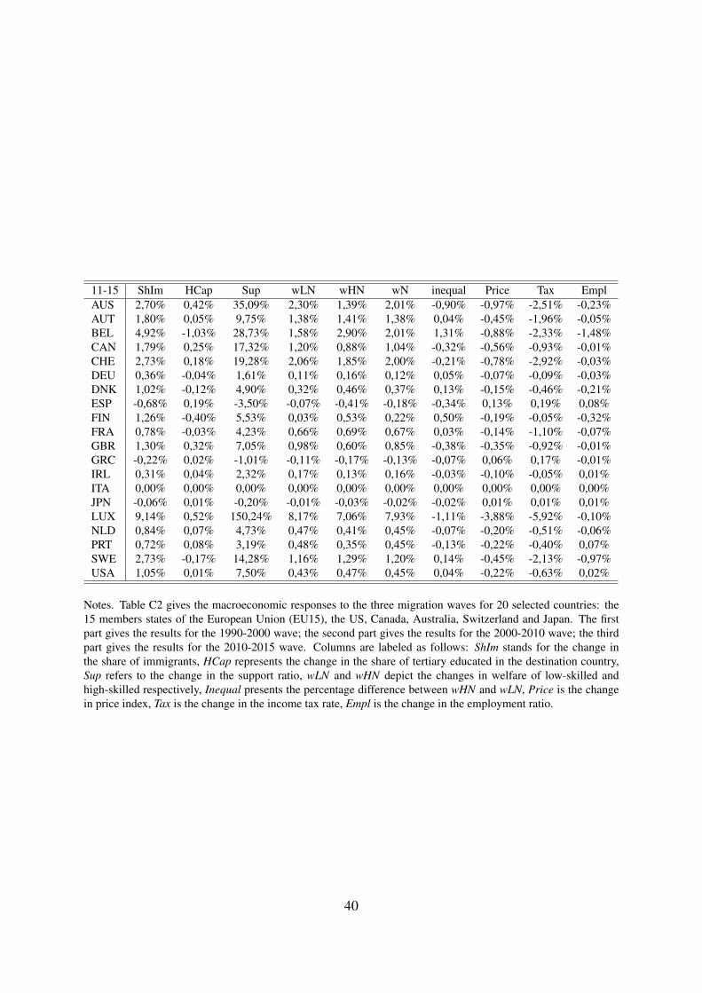
11-15 ShIm HCap Sup wLN wHN wN inequal Price Tax EmplAUS 2,70% 0,42% 35,09% 2,30% 1,39% 2,01% -0,90% -0,97% -2,51% -0,23%AUT 1,80% 0,05% 9,75% 1,38% 1,41% 1,38% 0,04% -0,45% -1,96% -0,05%BEL 4,92% -1,03% 28,73% 1,58% 2,90% 2,01% 1,31% -0,88% -2,33% -1,48%CAN 1,79% 0,25% 17,32% 1,20% 0,88% 1,04% -0,32% -0,56% -0,93% -0,01%CHE 2,73% 0,18% 19,28% 2,06% 1,85% 2,00% -0,21% -0,78% -2,92% -0,03%DEU 0,36% -0,04% 1,61% 0,11% 0,16% 0,12% 0,05% -0,07% -0,09% -0,03%DNK 1,02% -0,12% 4,90% 0,32% 0,46% 0,37% 0,13% -0,15% -0,46% -0,21%ESP -0,68% 0,19% -3,50% -0,07% -0,41% -0,18% -0,34% 0,13% 0,19% 0,08%FIN 1,26% -0,40% 5,53% 0,03% 0,53% 0,22% 0,50% -0,19% -0,05% -0,32%FRA 0,78% -0,03% 4,23% 0,66% 0,69% 0,67% 0,03% -0,14% -1,10% -0,07%GBR 1,30% 0,32% 7,05% 0,98% 0,60% 0,85% -0,38% -0,35% -0,92% -0,01%GRC -0,22% 0,02% -1,01% -0,11% -0,17% -0,13% -0,07% 0,06% 0,17% -0,01%IRL 0,31% 0,04% 2,32% 0,17% 0,13% 0,16% -0,03% -0,10% -0,05% 0,01%ITA 0,00% 0,00% 0,00% 0,00% 0,00% 0,00% 0,00% 0,00% 0,00% 0,00%JPN -0,06% 0,01% -0,20% -0,01% -0,03% -0,02% -0,02% 0,01% 0,01% 0,01%LUX 9,14% 0,52% 150,24% 8,17% 7,06% 7,93% -1,11% -3,88% -5,92% -0,10%NLD 0,84% 0,07% 4,73% 0,47% 0,41% 0,45% -0,07% -0,20% -0,51% -0,06%PRT 0,72% 0,08% 3,19% 0,48% 0,35% 0,45% -0,13% -0,22% -0,40% 0,07%SWE 2,73% -0,17% 14,28% 1,16% 1,29% 1,20% 0,14% -0,45% -2,13% -0,97%USA 1,05% 0,01% 7,50% 0,43% 0,47% 0,45% 0,04% -0,22% -0,63% 0,02%

Notes. Table C2 gives the macroeconomic responses to the three migration waves for 20 selected countries: the15 members states of the European Union (EU15), the US, Canada, Australia, Switzerland and Japan. The firstpart gives the results for the 1990-2000 wave; the second part gives the results for the 2000-2010 wave; the thirdpart gives the results for the 2010-2015 wave. Columns are labeled as follows: ShIm stands for the change inthe share of immigrants, HCap represents the change in the share of tertiary educated in the destination country,Sup refers to the change in the support ratio, wLN and wHN depict the changes in welfare of low-skilled andhigh-skilled respectively, Inequal presents the percentage difference between wHN and wLN, Price is the changein price index, Tax is the change in the income tax rate, Empl is the change in the employment ratio.

40