The changing dynamics of short-run output adjustment

Munich Personal RePEc Archive

The changing dynamics of short-run

output adjustment

Ertürk, Korkut Alp and Mendieta-Muñoz, Ivan

Department of Economics, University of Utah, Department of

Economics, University of Utah

5 June 2018

Online at https://mpra.ub.uni-muenchen.de/87409/

MPRA Paper No. 87409, posted 14 Jun 2018 21:38 UTC

1

THE CHANGING DYNAMICS OF SHORT-RUN

OUTPUT ADJUSTMENT

Korkut Alp Ertürk. Department of Economics, University of Utah. Office 240,

Building 73, 332 South 1400 East, Salt Lake City, Utah 84112, USA. Email:

[email protected]

Ivan Mendieta-Muñoz. Department of Economics, University of Utah. Office

213, Building 73, 332 South 1400 East, Salt Lake City, Utah 84112, USA. Email:

[email protected]

June 5, 2018

Abstract

Much of macroeconomic theorizing rests on assumptions that define the short-run output

adjustment of a mass-production economy. The demand effect of investment on output, assumed

much faster than its supply effect, works through employment expanding pari passu with changes

in capacity utilization while productivity remains constant. Using linear Structural VAR and Time-

Varying Parameter Structural VAR models, we document important changes in the short-run

output adjustment in the USA. The link between changes in employment, capacity utilization and

investment has weakened, while productivity became more responsive following demand shifts

caused by investment since the early 1990s.

JEL Classification: B50, E10, E32.

Keywords: changes in short-run output adjustment, capacity utilization, employment, mass-

production economy, post-Fordism.

2

1. Introduction

The paper discusses if some of macroeconomists’ theoretical priors still retain their relevance

today, presenting evidence that suggests they no longer might. The rise of mass production

economy in the manufacturing industry at the turn of the previous century had shaped many of the

building blocks of macroeconomic theorizing. However, not only manufacturing has shrunk

relative to other sectors in terms of its share of output (and in absolute terms in terms of

employment), but also its organization of production in advanced countries such as the USA has

long been transformed, altering the link between employment and output. When it comes to the

modality of this link, fixed productivity and variable capacity utilization/employment are,

according to Edward J. Nell’s succinct formulation, the defining characteristics of mass production

(Aglietta, 1979; Nell, 1992; Piore and Sable, 1984), which differ from the so-called craft system

with its fixed capacity utilization/employment and variable productivity. Ever since Piore and

Sable’s (1984) seminal work, it is commonly recognized that the rise of information technologies

may have revived the work pattern of a craft economy, and a large literature discusses the effect

this had on the rise of flexible specialization and employment (post-Fordism, for short).1

The present paper focuses on the implications of the latter for the short-run output

adjustment in the US economy. Using linear Structural Vector Autoregressive models and Time-

Varying Parameter Structural Vector Autoregressive models, we present evidence that the link

macroeconomists take for granted between changes in employment, capacity utilization and

investment has become weaker since the early 1990s; while productivity appears to have become

more responsive to demand shifts caused by investment. The results point out that the output

1See, among others, Jessop (1995, 2005) and Amin (1995) for a useful reader on post-Fordism. Closer to our paper

is discussions of Nell’s transformational growth in connection with business cycle dynamics –see, Nell & Phillips

(1995) and Ertürk (2004) for a formalization.

3

adjustment characteristic of the mass production system has lost some of its importance while that

depicting the craft production system has become more relevant.

Our contribution is also related to two strands of literature. First, the recent literature on

“jobless recoveries” (Burger & Schwartz, 2018; Chen & Cui, 2017; DeNicco & Laincz, 2018;

Panovska, 2017) has pointed out that the past three recoveries in the USA have been markedly

different from most postwar recoveries prior to 1990. In each successive episode, not only

employment continued to decline even as output began to revive but also permanent job losses

over temporary layoffs were higher. Although there is consensus in the literature regarding the

change in the dynamics of employment, there is no general consensus on the cause of jobless

recoveries. Several explanations for this change in the relationship between labor market variables

and output have been proposed in the theoretical literature, such as shifts across sectors and

occupations, employment overhang, changes in the persistence and amplitude in the output cycle,

and changes in the nature of the labor market, where demand shocks are absorbed on the intensive

margin (hours worked) or by using more flexible labor inputs.

Second, the observed weakening relationship between employment and output has also

raised questions about the stability of Okun’s Law. During the three most recent US recessions

and the Great Recession, the unemployment rate became much more sensitive to output growth

and output gap fluctuations than employment (Owyang and Sekhposyan, 2012; Elsby et al.,

2010). Different explanations have focused on aggressive job cutting by firms in part because of

deunionization and the diminished bargaining power of workers (Berger, 2012; Gordon, 2010),

changing industry composition (Basu & Foley, 2013), and labor reallocation (Garin et al., 2013).

Yet another view emphasized shifts in productivity growth (Daly & Hobjin, 2010) and the effect

of technological change on job polarization (Jaimovich & Siu, 2012; Siu and Jaimovich, 2015).

4

Although not inconsistent with any of these, our paper focuses more narrowly on whether

(or to what extent) the changing organization of work has blurred the distinction between fixed

and variable costs, lowering the importance of short-run output adjustments based on capacity

utilization variations and raising the one based on productivity fluctuations.

The following discussion is organized in three sections. Section 2 gives a conceptual

overview of craft and mass production systems and discusses the effect that the rise of mass

production had on the traditional conceptualization of output adjustment. Section 3 shows that the

empirical evidence supporting the conventional view of output adjustment based on the link

between employment, capacity utilization and investment has significantly weakened; while the

short-run responsiveness of productivity to investment has increased. The paper ends with a brief

conclusion presented in Section 4.

2. Craft and mass production systems

In a craft economy production is to order, and current costs are largely fixed. Work tends to be

specialized and requires teamwork. Being indispensable, each crew member needs to be present

for production to take place, which makes start-up and shut-down costs significant. The product is

customized (and thus non-standard) and few (if any) economies of scale exist. The system is highly

versatile in the face of shifts in demand and relative prices, and works well in the production of

non-standard, customized goods. However, craftsmen need a long time to acquire the prerequisite

level of skills, and thus can be a bottleneck in production. The dependence on teamwork is also a

constraint on output, with rising adjustment and coordination costs and diminishing returns that

quickly set in when the scale of production is increased (Nell, 1992).

5

Historically, these drawbacks gave an impetus to the switch to producing standardized

goods which were cheaper, although often inferior, substitutes for custom crafted goods. The cost

advantage was achieved by scale economies made possible by breaking down each complex task

performed by skilled workers to a series of routine tasks that could be performed by low skill

workers (Sokoloff, 1984). This also paved the way for the eventual introduction of machinery

since a mechanical arm could replace an organic one more easily if it performed a simple,

routinized task (Sherwood, 1985; MacKenzie, 1983). The new labor process inflexibly paired low

skills with routine tasks, replacing the fluid pairing of complex skills with variable tasks under the

craft economy. As a pre-designed sequence of routinized sub-tasks could become the unifying

thread of production, skilled craftsmen ceased to be indispensable. The resulting decrease in

requisite skill level in production made workers easily replaceable and the transformation of the

labor process eventually culminated in the rise of mass production and the modern assembly line.2

Unlike in a craft economy, economies of scale conferred competitive advantage on large

firms in mass production. The competitive pressures to better exploit it raised the minimum scale

of fixed investment over time, which meant increasingly long gestation periods before new plants

and equipment could begin operation. This in turn produced an inflexible structure of production

that became the soft belly of the system as the stable economic conditions that defined the “Golden

Age” began to unravel. The economic uncertainties of the 1970s –price volatility and increasingly

unpredictable fluctuations in consumer demand– raised the risk of large scale fixed investments.

As markets became more contingent and consumer demand more uncertain, the premium on

flexibility increased, undermining mass production. Economies scope became increasingly more

2Nevertheless, craft system was never completely superseded since mass production also had the effect of raising the

demand for a new breed of craftsmen such as engineers, designers and managers. The standardized goods that were

produced by low skill workers required product-specific, specialized machinery, which could not be mass produced

themselves.

6

important as competitive advantage accrued to those who could adjust their product mix swiftly

under rapidly changing conditions. Eventually, globalization carried off much of the old mass

production industries to developing countries leaving the “rustbelt” in its wake, while the diffusion

of information technologies had a radical effect on the labor process throughout the economy.

Even though little remains of the old mass production economy today, our idea of how short-run

output adjustment works still dates back from the time of its rise.

The importance of scale economies under mass production implied no natural size of

operations for firms and gave rise to oligopolistic markets. With firms building plants with reserve

capacity to administer prices, output, employment, and capacity utilization tended to vary pari

passu in response to changes in demand as labor productivity remained constant. Output moved

with demand as any change in autonomous spending gave rise to induced spending in the same

direction, while long gestation periods meant that the supply effect of fixed investment could safely

be ignored in the short run. Arguably, it was these patterns that tightly linked output adjustment to

changes in employment that moved with capacity utilization, responding to the demand shifts from

fixed investment.

Consider the equation that sets output equal to the product of labor productivity (𝜋) times

the quantity of labor employed (𝑁). Since by definition 𝜋 = 𝑌/𝑁, then

𝑌 = 𝜋𝑁 ……… (1)

It follows that the rate of change of output, d𝑌, is equal to:

d𝑌 = 𝜋d𝑁 + 𝑁d𝜋 ……… (2)

In the craft economy, output adjustment is based on variations in productivity where employment

remains mainly constant, which suggests that d𝑁 = 0. Therefore:

7

d𝑌 = 𝑁d𝜋 ……… (3)

By contrast, in a mass production economy, output adjustment is based on variations in

employment where productivity remains fixed. In other words, d𝜋 = 0, which gives:

d𝑌 = 𝜋d𝑁 ……… (4)

Capacity utilization (𝑣) plays an important role in this alternative specification. Again, by

definition, we have:

𝑌 = 𝑌𝑌∗ = 𝑣𝑌∗ ……… (5)

where 𝑌∗ is potential output. The change in output is now equal to:

d𝑌 = 𝑣d𝑌∗ + 𝑌∗d𝑣 ……… (6)

In mass production economy, the relatively long gestation period of fixed investments

conceptually defines the “short period” as the period long enough when the supply effect of

investment on capital stock –and thus on potential output– can be ignored, so that d𝑌∗ = 0 and

d𝑌 = 𝑌∗d𝑣 ……… (7)

Yet a third relation for changes in output is given by the Keynesian multiplier, tying it to shifts in

investment:

d𝑌 = 1𝑠 d𝐼 ……… (8)

where 𝑠 is the propensity to save/invest, and d𝐼 is the rate of change of saving/investment.

Putting all three together gives the conventional idea of short-run output adjustment that

characterizes the mass production system, where employment moves with changes in capacity

8

utilization that respond to autonomous shifts in aggregate demand. Therefore, combining equations

(4), (7) and (8) we have:

𝜋d𝑁 = 𝑌∗d𝑣 = 1𝑠 d𝐼

d𝑁 = 𝑌∗𝜋 d𝑣 = 1𝑠 d𝐼 ……… (9)

The underlying assumption in this conception is that both labor productivity and potential output

are invariant in the short run with respect to changes in investment. But, it is plausible that neither

assumption is as relevant today as it once was. At least in some sectors such as the manufacturing

industry, the prevalence of large fixed investments with long gestations periods might have

markedly decreased with the declining importance of economies scale.

If nimble firms that flexibly specialize in niche production are nearly as prevalent as

commonly argued in the post-Fordism literature, one would reasonably expect smaller scale

investments with shorter gestation periods on average and thus a shortening of the period long

enough when capacity can be safely assumed constant. Moreover, with much of technological

change embedded in new investment (as is especially the case with information technologies) the

effects on labor productivity can be discernible relatively quickly. Thus, the short run demand

effect of fixed investment might increasingly blend with its supply effect on capacity output and

productivity within the short period.3 This suggests an alternative form of output adjustment where

variable productivity rather than capacity utilization variations become important in a way that

3Although this cannot be pursued here, in related work we observe significant divergence across different sectors in

terms of their modality of output adjustment since the 1990s.

9

resembles the characteristic of a craft economy. Using equations (3), (6) and (8), this alternative

type of adjustment can be expressed as4:

d𝜋 = 𝑣𝑁 d𝑌∗ = 1𝑠 d𝐼 ……… (10) The evidence we present for the aggregate economy in the next section shows that the links

between investment and capacity utilization and between capacity utilization and employment

appear to have significantly weakened, and that the short run link between investment and

productivity has become stronger.

3. Empirical evidence

We estimate linear Structural Vector Autoregressive (SVAR) models and Time-Varying

Parameter SVAR (TVP-SVAR) models over different subperiods in order to study the changing

effects of investment on capacity utilization; capacity utilization on employment; and investment

on productivity. We focus on the interactions between the variables by presenting the Impulse-

response Functions (IRFs) derived from the identification strategies described in Section 3.2.

3.1 Data

Our data ranges from 1967Q1 until 2017Q4. The quarterly series were extracted from the National

Income and Product Accounts (NIPA) produced by the Bureau of Economic Analysis (BEA); the

Federal Reserve Database (Fed); the Federal Reserve Bank of St. Louis Economic Database

(FRED); and the Bureau of Labor Statistics (BLS).5

4Note that equation (10) uses the assumption that d𝑣 = 0 from equation (6) to represent the characteristics of a craft

economy. 5We also estimated the models without considering the end of sample instability generated by the Great Recession

and subsequent recovery. The results for the period 1967Q1-2007Q3 show even stronger responses of the relevant

10

The investment rate (𝑖𝑡) corresponds to the ratio of Private Fixed Investment to GDP (both

extracted from Table 1.1.5. Gross Domestic Product, NIPA). The capacity utilization rate (𝑣𝑡)

corresponds to the Fed’s total industry capacity utilization rate (extracted from Table G.17.

Industrial Production and Capacity Utilization).6 The employment rate corresponds to the civilian

employment rate (𝑛𝑡), defined as defined as 100 − 𝑢𝑡, where 𝑢𝑡 corresponds to the percent civilian

unemployment rate (extracted from the FRED database, UNRATE series).7 Finally, productivity

(𝜋𝑡) refers to the natural log of output per worker employed of the US business sector (extracted

from the BLS database).8

Figure 1 below plots the 𝑣𝑡 and 𝑖𝑡 series; and Figure 2 shows the 𝑛𝑡 and 𝑣𝑡 series. With

respect to the former, it is possible to observe that before the recessions of the early 1980s both

the 𝑣𝑡 and 𝑖𝑡 series tended to move together, but the relationship seems to have weakened since

then. The same holds true for the relationship between 𝑛𝑡 and 𝑣𝑡: before the crisis of the early

1990s, the 𝑛𝑡 and 𝑣𝑡 series tended to drop simultaneously during recessions and to increase during

expansions and were almost perfectly synchronized; however, the correlation between these

variables has become less pronounced since then.

relationships studied. Thus, although the Great Recession seems to have slightly modified the relevant correlations,

the overall patterns do not revert to early sample estimates. These results are available on request. 6We deem that the measure of 𝑣𝑡 published by the Fed captures more adequately the concept of capacity utilization

that we are interested in since it refers to the percentage of resources used by corporations and factories to produce

goods in manufacturing, mining, and electric and gas utilities for all facilities located in the USA (excluding those in

U.S. territories). As a robustness check, however, we also report the results obtained using a measure of 𝑣𝑡 constructed

using the Hamilton (2018) filter. These results are presented in Section 3.4. 7We also used the 𝑛𝑡 for prime-age workers (ages 25-54, extracted from the FRED database, LREM25TTUSM156S

series). The results obtained corroborate the main findings and are available on request. 8Strictly speaking, the constructed indicator of productivity corresponds to a measure of output per job since we

divided the business sector’s output indicator (PRS84006043 series) by the business sector’s employment indicator (PRS84006013 series) provided by the BLS. We tried to measure productivity as output per worker (instead of output

per hour) to avoid the possible effects on hours worked. Nevertheless, the results obtained using the business sector’s output per hour as a measure of productivity also corroborate the main findings (once again, these results are available

on request).

11

[INSERT FIGURE 1 ABOUT HERE]


3.2 SVAR models

The short-run output adjustment associated with the mass production system (MPS) can be studied

by presenting the dynamic interactions between 𝑖𝑡, 𝑣𝑡, and 𝑛𝑡. On the other hand, the short-run

output adjustment that depicts the craft production system (CPS) can be studied by presenting the

interactions between 𝑖𝑡, 𝑣𝑡, and 𝜋𝑡. We compare the IRFs obtained from both models over different

subperiods.

First, we carried out different unit root tests to study the order of integration of the series,

finding that the 𝑖𝑡, 𝑣𝑡, and 𝑛𝑡 are stationary processes, that is, 𝐼(0); and that 𝜋𝑡 is a non-stationary

series integrated of order 1, that is, 𝐼(1).9 Hence, in order to estimate Vector Autoregressive

(VAR) models in which the variables have the same order of integration we included 𝑖𝑡, 𝑣𝑡, and 𝑛𝑡 for the MPS; and 𝑖𝑡, 𝑣𝑡, and Δ𝜋𝑡 for the CPS (where Δ denotes the first differences).10

The estimated VAR models adopted the following general form:

y𝑡 = C0 + ∑C𝑖y𝑡−𝑖𝑝𝑖−1 + 𝑢𝑡 ……… (11)

Ay𝑡 = A0 + ∑A𝑖y𝑡−𝑖𝑝𝑖−1 + B𝜀𝑡 ……… (12)

where equation (11) represents the reduced-form VAR and equation (12) shows the SVAR model;

and 𝑢𝑡 and 𝜀𝑡 are white-noise vector processes with 𝑢𝑡~𝑁(0, 𝐼) and 𝜀𝑡~𝑁(0, Σ), respectively. The

vector y𝑡 contains either 𝑖𝑡, 𝑣𝑡 and 𝑛𝑡 to characterize the short-run output adjustment associated

9A full description of the results obtained from the different unit root tests is available on request. 10Specifically, we considered Δ𝜋𝑡 = 100 ∗ (𝜋𝑡 − 𝜋𝑡−1).

12

with the MPS or 𝑖𝑡, 𝑣𝑡 and Δ𝜋𝑡 to characterize the short-run output adjustment of the CPS. This

leads to the well-known identification problem for both cases: recovering the SVAR models in

equation (12) from the estimated reduced-form models shown in equation (11).

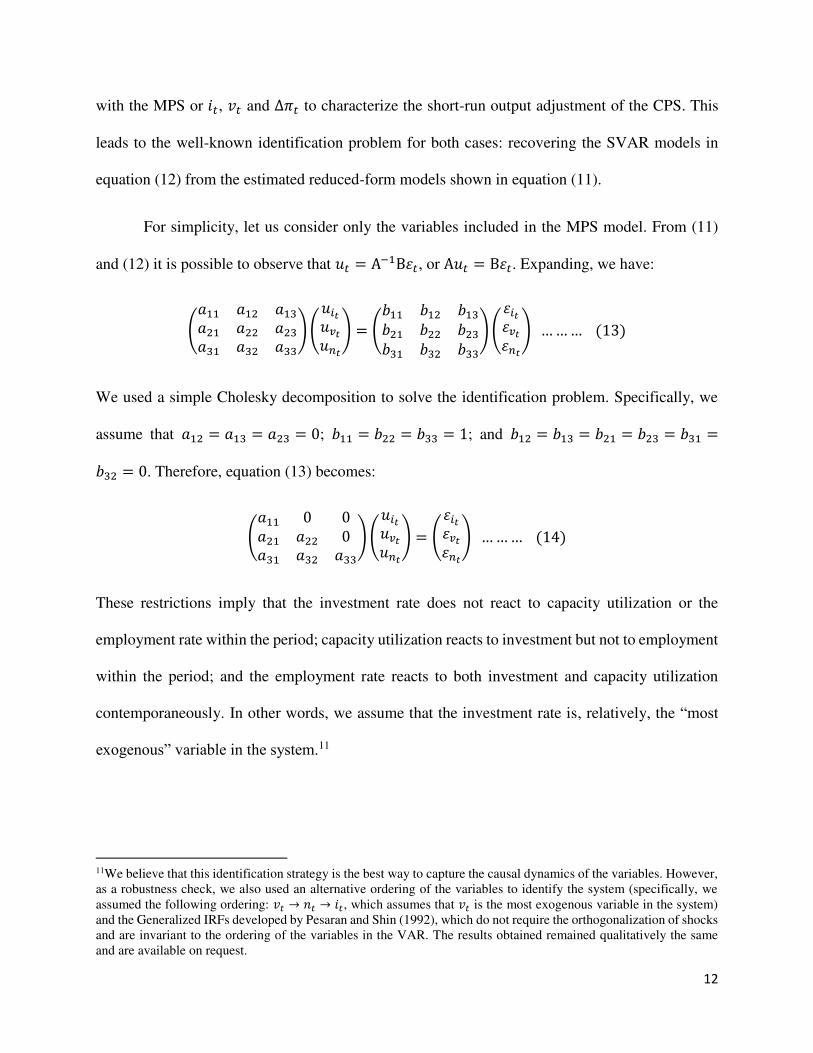
For simplicity, let us consider only the variables included in the MPS model. From (11)

and (12) it is possible to observe that 𝑢𝑡 = A−1B𝜀𝑡, or A𝑢𝑡 = B𝜀𝑡. Expanding, we have:

(𝑎11 𝑎12 𝑎13𝑎21 𝑎22 𝑎23𝑎31 𝑎32 𝑎33)(𝑢𝑖𝑡𝑢𝑣𝑡𝑢𝑛𝑡) = (𝑏11 𝑏12 𝑏13𝑏21 𝑏22 𝑏23𝑏31 𝑏32 𝑏33)(𝜀𝑖𝑡𝜀𝑣𝑡𝜀𝑛𝑡) ……… (13)

We used a simple Cholesky decomposition to solve the identification problem. Specifically, we

assume that 𝑎12 = 𝑎13 = 𝑎23 = 0; 𝑏11 = 𝑏22 = 𝑏33 = 1; and 𝑏12 = 𝑏13 = 𝑏21 = 𝑏23 = 𝑏31 =𝑏32 = 0. Therefore, equation (13) becomes:

(𝑎11 0 0𝑎21 𝑎22 0𝑎31 𝑎32 𝑎33)(𝑢𝑖𝑡𝑢𝑣𝑡𝑢𝑛𝑡) = (𝜀𝑖𝑡𝜀𝑣𝑡𝜀𝑛𝑡) ……… (14)

These restrictions imply that the investment rate does not react to capacity utilization or the

employment rate within the period; capacity utilization reacts to investment but not to employment

within the period; and the employment rate reacts to both investment and capacity utilization

contemporaneously. In other words, we assume that the investment rate is, relatively, the “most

exogenous” variable in the system.11

11We believe that this identification strategy is the best way to capture the causal dynamics of the variables. However,

as a robustness check, we also used an alternative ordering of the variables to identify the system (specifically, we

assumed the following ordering: 𝑣𝑡 → 𝑛𝑡 → 𝑖𝑡, which assumes that 𝑣𝑡 is the most exogenous variable in the system)

and the Generalized IRFs developed by Pesaran and Shin (1992), which do not require the orthogonalization of shocks

and are invariant to the ordering of the variables in the VAR. The results obtained remained qualitatively the same

and are available on request.

13

Likewise, we also employed a similar identification strategy for the variables included in

the CPS model:

(𝑎11 0 0𝑎21 𝑎22 0𝑎31 𝑎32 𝑎33)( 𝑢𝑖𝑡𝑢𝑣𝑡𝑢Δ𝜋𝑡) = ( 𝜀𝑖𝑡𝜀𝑣𝑡𝜀Δ𝜋𝑡) ……… (15)

The restrictions imposed in (15) imply that the investment rate does not react to capacity

utilization or productivity contemporaneously; capacity utilization reacts to investment but not to

productivity within the period; and that productivity reacts to both investment and capacity

utilization within the period.

To summarize, the key difference between equations (14) and (15) is the inclusion of Δ𝜋𝑡 instead of 𝑛𝑡, which allows us to distinguish between the short-run adjustment characteristic of the

CPS and MPS, respectively. With respect to the MPS, our main interest consists in evaluating if

the responses of 𝑣𝑡 to 𝑖𝑡 shocks and of 𝑛𝑡 to 𝑣𝑡 shocks have decreased over time. Regarding the

CPS, we are interested in testing if the response of 𝑣𝑡 to 𝑖𝑡 shocks has decreased over time and if

the response of Δ𝜋𝑡 to 𝑖𝑡 shocks has increased over time.

3.3 Results

The SVAR models that depict the MPS and the CPS were estimated over two different subsamples,

1967Q1-1992Q3 and 1992Q4-2017Q4. We selected these two periods because each one of them

contains approximately 50% of the observations of the whole sample. More importantly, we

corroborated the appropriateness of this sample splitting approach using a Likelihood Ratio test,

thus testing for the presence of a structural break in the VAR models.

Following Lütkepohl (2006), the Likelihood Ratio statistic (𝜆LR) can be constructed as

follows: 𝜆LR = 2 ∗ (𝜆U − 𝜆R), where 𝜆U is the log-likelihood obtained from the unrestricted VAR

(sum of the log-likelihoods estimated from the VAR models considering two different periods,

14

1967Q1-1992Q3 and 1992Q4-2014Q4) and 𝜆R is the log-likelihood obtained from the restricted

VAR (obtained from the VAR model considering only one period, 1967Q1-2014Q4). Under the

null hypothesis that the dataset can be represented by a single VAR (that is, there is no structural

change)12, the 𝜆LR has an asymptotic 𝜒2-distribution with degrees of freedom (𝑚) equal to the

number of linearly independent restrictions.13 If 𝜆LR > 𝜒2(𝑚) then the null hypothesis is rejected.

Table 1 below summarizes the results. It is possible to observe that the null hypothesis of

no structural change is rejected at the 5% level for the VAR models that depict both the MPS and

the CPS. Hence, there is evidence of a structural break in the VAR models, and it is appropriate to

divide the sample into two subperiods.

[INSERT TABLE 1 ABOUT HERE]

Figures 3 and 4 below present the most relevant IRFs for both periods. The former presents the

results for the MPS, and the latter presents the ones obtained from the CPS.14



With respect to short-run output adjustment characteristic of the MPS, it is possible to

observe that the response of 𝑣𝑡 to 𝑖𝑡 shocks is considerable lower in the second period. In the same

vein, the response of 𝑛𝑡 to 𝑣𝑡 shocks is also lower during the period 1992Q4-2017Q4 than during

the period 1967Q1-1992Q3.

12In brief, this approach tests the null hypothesis that all coefficients are time-invariant against the alternative that the

white-noise covariance matrix is time invariant while the rest of the coefficients vary across subsamples (see

Lütkepohl, 2006). 13Therefore, 𝑚 = (𝑠 − 1)𝑘(𝑘𝑝 + 1), where 𝑠 is the number of subperiods considered, and 𝑘 and 𝑝 are the number of

variables and the number of lags included in the restricted VAR, respectively. 14A complete report showing the different responses of all variables to all shocks in the respective systems is available

on request.

15

On the other hand, from the short-run output adjustment associated with the CPS it is

possible to observe that the response of 𝑣𝑡 to 𝑖𝑡 shocks is also lower in the second period and the

response of 𝜋𝑡 to 𝑖𝑡 shocks is both statistically significant and larger during the period 1992Q4-

2017Q4 compared to the period 1967Q1-1992Q3.

In order to summarize the main findings, Figure 5 compares only the mean responses

(without confidence intervals) of the variables for both periods.


The main results can be summarized as follows. From the MPS we can conclude that: 1) a

1 percentage point shock to 𝑖𝑡 increased 𝑣𝑡 by approximately 0.49 percentage points during the

period 1967Q1-1992Q3 and by approximately 0.25 percentage points during the period 1992Q4-

2017Q4; and 2) a 1 percentage point shock to 𝑣𝑡 increased 𝑛𝑡 by approximately 0.18 percentage

points during the period 1967Q1-1992Q3 and by approximately 0.09 percentage points during the

period 1992Q4-2017Q4.

On the other hand, the results for the CPS show that a 1 percentage point shock to 𝑖𝑡 increased 𝑣𝑡 by approximately 0.55 percentage points during the period 1967Q1-1992Q3 and by

approximately 0.21 percentage points during the period 1992Q4-2017Q4. More importantly, the

contemporaneous response of Δ𝜋𝑡 to a 1 percentage point shock to 𝑖𝑡 is statistically non-significant

in the first period; however, during the period 1992Q4-2017Q4 the response of Δ𝜋𝑡 to 𝑖𝑡 becomes

statistically significant: a 1 percentage point shock to 𝑖𝑡 increased productivity growth by

approximately 0.15 percentage points.

As an alternative to estimating linear VAR models over two different subsamples, we also

performed the estimation of TVP-SVAR models developed by Primiceri (2005) and Del Negro

and Primiceri (2015). One of the main advantages of this methodology is that it represents a

16

multivariate time series technique with both time-varying parameters and time-varying covariance

matrix of the additive innovations. This is done by allowing the model parameters and the entire

variance covariance matrix of the shocks to evolve smoothly over time. The drifting coefficients

allows us to capture possible non-linearities or time-variation in the lag structure of the model;

whereas the multivariate stochastic volatility is meant to capture possible heteroskedasticity of the

shocks and non-linearities in the simultaneous relations among the variables of the model.15

Figure 6 summarizes the most important IRFs for both the MPS and CPS models.16 The

TVP-SVAR models generate IRFs at every single data point, so reporting the full set becomes a

challenge. The dates chosen for the comparison were 1977Q3 (1978Q3) for the MPS (for the CPS)

and 2004Q4, which approximately correspond to middle dates between the first and last NBER

trough and peak dates included: 1975Q1-1980Q1 and 2001Q4-2007Q4.17


It is possible to observe that the results obtained from the TVP-SVARs corroborate the

ones obtained from the linear SVARs. With respect to the MPS, the response of 𝑣𝑡 to a 1 percentage

point increase in 𝑖𝑡 was 0.31 percentage points in 1977Q3 and 0.25 percentage points in 2004Q4;

and the response of 𝑛𝑡 to a 1 percentage point increase in 𝑣𝑡 was 0.11 in 1977Q3 and 0.10 in

2004Q4. Regarding the CPS, a 1 percentage point increase in 𝑖𝑡 increased 𝑣𝑡 by around 0.30

15Appendix A contains a description of the most important technical aspects of TVP-SVAR models. 16For simplicity, Figure 5 only reports a summary of the IRFs. A more complete set of results is presented in Appendix

B. Figures B.1 and B.2 report the stochastic volatility parameters and the IRFs together with their respective

confidence intervals for the MPS; and Figures B.3 and B.4 show the results for the CPS. It is worth noting that the

stochastic volatility coefficients estimated for both models show a clear downward trend, which corroborates one of

the findings of the literature on the Great Moderation (that is, a reduction in the volatility of business cycle

fluctuations).

17Note that the first 10 years of observations are “not available” because these are used for the initialization of the prior (see Appendix A). Note also that, with respect to the CPS, less observations are available because of the use of

the first-differences of the log of productivity. Therefore, we selected the one-year later date, 1978Q3, instead of

1977Q3. It is also worth mentioning that experiments with different dates for the MPS and CPS over the periods

1975Q1-1980Q1 and 2001Q4-2007Q4 give very similar conclusions.

17

percentage points and had no significant effect on Δ𝜋𝑡 in 1978Q3; whereas it increased 𝑣𝑡 by

around 0.19 percentage points and had a statistically significant effect on Δ𝜋𝑡 of approximately

0.06 percentage points in 2004Q4 (after one quarter).

Hence, it is possible to say that the responses of 𝑣𝑡 to 𝑖𝑡 and of 𝑛𝑡 to 𝑣𝑡 have decreased

since the early 1990s and that the response of Δ𝜋𝑡 to 𝑖𝑡 has increased since then. In other words,

the short-run output adjustment characteristic of the MPS has become less important and the one

characteristic of the CPS has become more relevant.

3.4 Robustness of results

As an alternative to the Fed’s 𝑣𝑡, we also used a measure of 𝑣𝑡 constructed as 100 ∗ (𝑦𝑡 − 𝑦𝑡∗),

where 𝑦𝑡 corresponds to the natural log of Real GDP (extracted from the FRED database, GDPC1

series) and 𝑦𝑡∗ corresponds to the natural log of the trend component of 𝑦𝑡 obtained using the

method proposed by Hamilton (2018). Hamilton (2018) has recently criticized the use of the

Hodrick and Prescott (1997) and has developed an alternative methodology that consists in using

simple forecasts of the series to remove the cyclical component.18 Therefore, the 𝑦𝑡∗ series

corresponds to a smoothed estimate of 𝑦𝑡 generated using the fitted values from a regression of the

latter on 4 lagged values of 𝑦𝑡 back-shifted by two years (that is, 8 observations in quarterly data)

and a constant: 𝑦𝑡 = 𝛽0 + 𝛽1𝑦𝑡−8 + 𝛽2𝑦𝑡−9 + 𝛽3𝑦𝑡−10 + 𝛽3𝑦𝑡−11 + 𝑒𝑡, where 𝑒𝑡 denotes the

residuals of this regression.

18The use of the Hodrick-Prescott filter has been criticized by Hamilton (2018) because: 1) it produces series with

spurious dynamic relations that have no basis in the underlying data-generating process; 2) filtered values at the end

of the sample are very different from those in the middle and are also characterized by spurious dynamics; and 3) a

statistical formalization of the problem typically produces values for the smoothing parameter vastly at odds with

common practice.

18

Figure 7 below plots the two different measures of 𝑣𝑡, and we also compare them with a

measure of utilization generated considering 𝑦𝑡∗ as the trend component obtained from the Hodrick

and Prescott filter (1997).19 Although the three measures of 𝑣𝑡 present similar movements over

the business cycle, only the Fed’s measure of 𝑣𝑡 and the one generated using Hamilton’s method

present a statistically significant downward trend.20 Given the drawbacks associated with the

Hodrick-Prescott filter, we only report the results obtained using Hamilton’s method.21


Figure 8 summarizes the most important results obtained from the linear SVAR models for

the periods 1967Q1-1992Q3 and 1992Q4-2017Q4; and Figure 9 presents the IRFs obtained from

the TVP-SVARs.22 It is possible to observe that both the SVAR and TVP-SVAR models show that

the response of 𝑣𝑡 to 𝑖𝑡 is lower in the second period compared to the first period. This result takes

place both in the MPS and CPS models. The contemporaneous response of 𝑛𝑡 to 𝑣𝑡 is lower in the

second period when the MPS is considered, although its response is statistically significantly

higher during two more quarters according to the linear SVAR models. Finally, with respect to the

CPS model, the response of Δ𝜋𝑡 to a 1 percentage point increase in 𝑖𝑡 is statistically significant in

the second period during approximately two quarters (one quarter) when the SVAR (when the

19The 𝑦𝑡∗ series obtained using Hamilton’s method and the Hodrick-Prescott filter (in which the smoothing parameter

was selected to be 1600 since we have quarterly data) were generated for the period 1948Q1-2017Q4, but we only

considered the period 1967Q1-2017Q4 to compare them with the Fed’s measure of 𝑣𝑡. 20This is corroborated by different unit root tests, which show that the Fed’s 𝑣𝑡 and the one constructed using

Hamilton’s method are trend stationary series, and the 𝑣𝑡 derived from the use of the Hodrick-Prescott filter is simply

a stationary series. (Results are available on request). 21The results obtained using the Hodrick-Prescott filter are also available on request. In brief, the main results are also

corroborated when we used this filtering technique, the only exception being the response of productivity to investment

shocks. 22We only present the mean responses of the relevant variables and refer to the significance of the estimates without

presenting the respective confidence intervals. A full report that also includes the latter is available on request.

19

TVP-SVAR) model was used; and it was found to be statistically non-significant during the first

period.



Hence, although less drastic, the results obtained using this alternative measure of 𝑣𝑡

corroborate the ones derived from the use of the Fed’s measure of 𝑣𝑡. The short-run adjustment

characteristic of the MPS has lost some of its importance since the early 1990s, and the output

adjustment characteristic of the CPS has gained importance since then.

4 Conclusions

The traditional idea of short period output adjustment rests on the assumption that the demand

effect of investment is almost immediate while its supply effect comes much later. In an economy

not constrained by full employment or capacity, output response to demand stimuli during this

short period is thought to derive from employment that expands pari passu with changes in

capacity utilization while productivity remains constant. These ideas, which remain foundational

for much contemporary macroeconomic theorizing, characteristically define a mass production

economy.

In this paper, we hypothesized that the eclipse of mass production in advanced economies

such as the USA is what lies at the bottom of the widely observed weakened link between

employment and output since the early 1990s. Asking whether the link between changes in

employment, capacity utilization and investment has changed over time, we empirically

investigated the effect of mass production system’s decline on short run output adjustment. Using

linear Structural Vector Autoregressive models and Time-Varying Parameter Structural Vector

20

Autoregressive models, we found that capacity utilization variations have become progressively

less sensitive while productivity became more responsive to demand shifts caused by investment

since the early 1990s. These results point out an important change in the short-run output

adjustment for the US economy, thus suggesting that the one associated with a mass production

economy has weakened and the one characteristic of a craft production system has become more

relevant.

Our findings might be capturing not only economy wide behavioural changes, but also

compositional effects caused by increased sectoral differences, which we have not examined in

this paper. We hope that our paper will inspire other researchers to study if and how short-run

output adjustment might have diverged across different sectors of the economy.

21

65

70

75

80

85

90

12

14

16

18

20

22

70 75 80 85 90 95 00 05 10 15

Capacity utilization rate (Federal Reserve; left axis)

Investment rate (right axis)

Figure 1. USA, 1967Q1-2017Q4. Capacity utilization and investment rates. (Shaded areas

indicate NBER recession dates.)

88

90

92

94

96

98

65

70

75

80

85

90

70 75 80 85 90 95 00 05 10 15

Employment rate (left axis)

Capacity utilization rate (Federal Reserve; right axis)

Figure 2. USA, 1967Q1-2017Q4. Employment and capacity utilization rates. (Shaded areas

indicate NBER recession dates.)

22

Table 1. Likelihood ratio tests for structural breaks in the VAR modelsa

𝜆s1b 𝜆s2b 𝜆Ub 𝜆Rb 𝜆LRb 𝜒2(𝑚)b

VAR models for the

mass production

system (including 𝑖𝑡, 𝑛𝑡 and 𝑣𝑡)

-109.83 23.58 -86.25 -131.43 90.36 54.57

VAR models for the

craft production

system (including 𝑖𝑡, 𝑛𝑡 and Δ𝜋𝑡) -239.41

-102.75

-342.16 -405.24 126.15 54.57

Notes: aThe optimal lag length for the VAR models was selected according to the Schwarz

information criterion. However, most of these models presented serial correlation problems

at the 5% level, so it was necessary to increase the number of lags. The restricted VARs

both for the mass and craft production systems included 4 lags. The unrestricted VAR for

the mass production system included 2 and 4 lags in the first and second periods,

respectively. The unrestricted VAR for the craft production system included 3 and 6 lags in

the first and second periods, respectively. b𝜆s1: Log-likelihood for the first period, 1967Q1-

1992Q3; 𝜆s2: Log-likelihood for the second period, 1992Q4-2017Q4; 𝜆U = 𝜆s1 + 𝜆s2: Log-

likelihood for the unrestricted VAR; 𝜆R: Log-likelihood of the restricted VAR; 𝜆LR = 2 ∗(𝜆U − 𝜆R): Likelihood ratio statistic; 𝜒2(𝑚): Critical value of the 𝜒2 distribution at the 5%

level with 𝑚 = (𝑠 − 1)𝑘(𝑘𝑝 + 1) = 39 degrees of freedom, where 𝑠 = 2, 𝑘 = 3 and 𝑝 =4 denote the number of subperiods considered, and the number of variables and lags in the

restricted VAR, respectively.

23

-0.8

-0.4

0.0

0.4

0.8

1.2

2 4 6 8 10 12 14 16 18 20

-.2

.0

.2

.4

2 4 6 8 10 12 14 16 18 20

(a) Response of 𝑣𝑡 to an 𝑖𝑡 shock, (b) Response of 𝑛𝑡 to a 𝑣𝑡 shock,

period 1967Q1-1992Q3 period 1967Q1-1992Q3

-0.5

0.0

0.5

1.0

1.5

2 4 6 8 10 12 14 16 18 20

-.4

-.2

.0

.2

.4

2 4 6 8 10 12 14 16 18 20

(c) Response of 𝑣𝑡 to an 𝑖𝑡 shock, (d) Response of 𝑛𝑡 to a 𝑣𝑡 shock,


Figure 3. Impulse-response functions obtained from the SVAR models that represent the mass

production system’s short-run output adjustment. The VARs for the periods 1967Q1-1992Q3

and 1992Q4-2017Q4 included 2 and 4 lags, respectively. These VAR models did not present

problems of serial correlation at the 5% level. The estimated VAR for the period 1992Q4-

2017Q4 included an exogenous trend since it was found to be jointly significant according to a

Wald coefficient test. Notation: 𝑣𝑡 = capacity utilization rate; 𝑖𝑡 = investment rate; and 𝑛𝑡 =

employment rate. Dotted lines are the 95% confidence intervals generated via 2,000 Monte Carlo

simulations

24

-0.5

0.0

0.5

1.0

1.5

1 2 3 4 5 6 7 8 9 10

-.2

.0

.2

.4

1 2 3 4 5 6 7 8 9 10

(a) Response of 𝑣𝑡 to an 𝑖𝑡 shock, (b) Response of Δ𝜋𝑡 to an 𝑖𝑡 shock,


-0.5

0.0

0.5

1.0

2 4 6 8 10 12 14 16 18 20

-.3

-.2

-.1

.0

.1

.2

.3

2 4 6 8 10 12 14 16 18 20

(c) Response of 𝑣𝑡 to an 𝑖𝑡 shock, (d) Response of Δ𝜋𝑡 to an 𝑖𝑡 shock,


Figure 4. Impulse-response functions obtained from the SVAR models that represent the craft

production system’s short-run output adjustment. The VARs for the periods 1967Q1-1992Q3

and 1992Q4-2017Q4 included 3 and 6 lags, respectively. These VAR models did not present

problems of serial correlation at the 5% level. The estimated VAR for the period 1992Q4-

2017Q4 included an exogenous trend since it was found to be jointly significant according to a

Wald coefficient test. Notation: 𝑣𝑡 = capacity utilization rate; 𝑖𝑡 = investment rate; and Δ𝜋𝑡 =

first differences of the natural log of productivity. Dotted lines are the 95% confidence intervals

generated via 2,000 Monte Carlo simulations

25

(a) Responses of 𝑣𝑡 to an 𝑖𝑡 shock, (b) Responses of 𝑛𝑡 to a 𝑣𝑡 shock,

mass production system (Figure 3) mass production system (Figure 3)

(c) Responses of 𝑣𝑡 to an 𝑖𝑡 shock, (d) Responses of Δ𝜋𝑡 to an 𝑖𝑡 shock,

craft production system (Figure 4) craft production system (Figure 4)

Figure 5. Summary of the impulse-response functions presented in Figures 3 and 4. Straight

lines are the mean responses for the period 1967Q1-1992Q3. Dotted lines are the mean responses

for the period 1992Q4-2017Q4. Notation: 𝑣𝑡 = capacity utilization rate; 𝑖𝑡 = investment rate; 𝑛𝑡 = employment rate; and Δ𝜋𝑡 = first differences of the natural log of productivity.

26

-.2

.0

.2

.4

.6

.8

2 4 6 8 10 12 14 16 18 20.00

.05

.10

.15

.20

.25

.30

2 4 6 8 10 12 14 16 18 20


mass production system mass production system

-.2

.0

.2

.4

.6

.8

2 4 6 8 10 12 14 16 18 20-.03

-.02

-.01

.00

.01

.02

.03

.04

.05

.06

2 4 6 8 10 12 14 16 18 20


craft production system craft production system

Figure 6. Summary of the impulse-response functions for the TVP-SVAR models. Straight lines

are the mean responses in 1977Q3 (mass production system) or 1978Q3 (craft production

system). Dotted lines are the mean responses in 2004Q4. Notation: 𝑣𝑡 = capacity utilization rate; 𝑖𝑡 = investment rate; 𝑛𝑡 = employment rate; and Δ𝜋𝑡 = first differences of the natural log of

productivity.

27

65

70

75

80

85

90

-5

0

5

10

15

70 75 80 85 90 95 00 05 10 15

Federal Reserve (left axis)

Hamilton filter (right axis)

Hodrick-Prescott filter (right axis)

Figure 7. USA, 1967Q1-2017Q4. Capacity utilization rates. (Shaded areas indicate NBER

recession dates.)

28



(c) Responses of 𝑣𝑡 to an 𝑖𝑡 shock, (d) Response of Δ𝜋𝑡 to an 𝑖𝑡 shock,


Figure 8. Summary of the impulse-response functions for the SVAR models using the measure

of 𝑣𝑡 derived from Hamilton’s filter. Straight lines are the mean responses for the period

1967Q1-1992Q3. Dotted lines are the mean responses for the period 1992Q4-2017Q4. The

estimated VARs for the period 1992Q4-2017Q4 included an exogenous trend since it was found

to be jointly significant according to a Wald coefficient test. Notation: 𝑣𝑡 = capacity utilization

rate; 𝑖𝑡 = investment rate; 𝑛𝑡 = employment rate; and Δ𝜋𝑡 = first differences of the natural log

of productivity.

29

-.2

.0

.2

.4

.6

.8

2 4 6 8 10 12 14 16 18 20.00

.05

.10

.15

.20

.25

2 4 6 8 10 12 14 16 18 20



-.2

.0

.2

.4

.6

.8

2 4 6 8 10 12 14 16 18 20-.04

.00

.04

.08

.12

2 4 6 8 10 12 14 16 18 20



Figure 9. Summary of the impulse-response functions for the TVP-SVAR models using the

measure of 𝑣𝑡 derived from Hamilton’s filter. Straight lines are the mean responses in 1977Q3

(mass production system) or 1978Q3 (craft production system). Dotted lines are the mean

responses for 2004Q4. Notation: 𝑣𝑡 = capacity utilization rate; 𝑖𝑡 = investment rate; 𝑛𝑡 =

employment rate; and Δ𝜋𝑡 = first differences of the natural log of productivity.

30

Acknowledgements

We are grateful to Minqui Li, Codrina Rada, Rudiger von Arnim, and seminar participants at the

University of Utah for helpful comments on a previous version of this paper. All errors are the

authors’ responsibility.

31

References

Aglietta, M. (1979). A Theory of Capitalist Regulation: The US Experience. London: Verso.

Amin, A. (1994). (Ed.) Post-Fordism: A Reader. Oxford: Blackwell Publishers.

Basu, D. & Foley, D. (2013). Dynamics of output and employment in the US economy. Cambridge

Journal of Economics, 37, 1077-1106.

Berger, D. (2012). Countercyclical Restructuring and Jobless Recoveries. Society for Economic

Dynamics, 2012 Meeting Papers, No. 1179.

Burger, J. & Schwartz, J. (2018). Jobless recoveries: Stagnation or structural change? Economic

Inquiry, 56, 709-723.

Chen. L. & Cui, Z. (2017). Jobless recovery and structural change: A VAR approach. South Asian

Journal of Macroeconomics and Public Finance, 6, 1-26.

Daly, M. & B. Hobijn (2010). Okun’s law and unemployment surprise of 2009. Federal Reserve

Bank of San Francisco Economic Letter, March 8, 1-4.

Del Negro, M. & Primiceri, G. (2015). Time varying structural vector autoregressions and

monetary policy: A corrigendum. Review of Economic Studies, 82, 1342-1342.

DeNicco, J. & Laincz, C. (2018). Jobless recovery: A time series look at the United States. Atlantic

Economic Journal, 46, 3-25.

Elsby, M., Hobijn, B & Şahin, A. (2010). The labor market in the Great Recession. Brookings

Papers on Economic Activity, 41, 1-69.

Ertürk, K. (2004). Transformational growth and the changing nature of the business cycle. In

Argyrous, G., Mongiovi, G. & Forstater, M. (Eds.) Growth, Distribution and Effective

https://ideas.repec.org/s/red/sed012.html

32

Demand. Alternatives to Economic Orthodoxy: Essays in Honor of Edward J. Nell. New

York: M. E. Sharpe, pp. 23-34.

Garin, J., Pries, M. & Sims, E. (2013). Reallocation and the changing nature of economic

fluctuations. University of Notre Dame, Mimeo.

Gordon, R. J. (2010). Okun’s Law and Productivity Innovations. American Economic Review,

Papers & Proceedings, 100, 11-15.

Hamilton, J. (2018). Why you should never use the Hodrick-Prescott filter. Review of Economics

and Statistics. Forthcoming.

Hodrick, R. & Prescott, E. (1997). Postwar U.S. business cycles: An empirical investigation.

Journal of Money, Credit, and Banking, 29, 1-16.

Jaimovich, N. & Siu, H. (2012). The trend is the cycle: Job polarization and jobless recoveries.

NBER Working Paper, No. 18334.

Jessop, B. (1995). The regulation approach, governance and post-Fordism: Alternative

perspectives on economic and political change? Economy and Society, 24, 307-333.

Jessop, B. (2005). Fordism and post-Fordism: A critical reformulation. In Storper, M. & Scott,

A.J. (Eds). Pathways to Industrialization and Regional Development. London: Routledge,

pp. 42-62.

Lütkepohl, H. (2006). New Introduction to Multiple Time Series Analysis. Berling, Heidelberg:

Springer-Verlag.

MacKenzie, D. (1983). Marx and the Machine. Technology and Culture, 25, 473-502.

33

Nell, E.J. (1992). Transformational Growth and Effective Demand. Economics After the Capital

Critique. New York: New York University Press.

Nell, E.J. & Phillips, T.F. (1995). Transformational growth and the business cycle. Eastern

Economic Journal, 21, 125-146.

Nell, E.J. (1998). Stages in the development of the business cycle. In Hagemann, H. and Kurz, H.

(Eds). Political economics in retrospect: Essays in memory of Adolph Lowe. Cheltenham:

Edward Elgar, pp. 131-154.

Owyang, M. & Sekhposyan, T. (2012). Okun’s law over the business cycle: Was the Great

Recession all that different? Federal Reserve Bank of St. Louis Review, 94, 399-418.

Panovska, I. (2017). What explains the recent jobless recoveries? Macroeconomic Dynamics, 21,

708-732.

Pesaran, H. & Shin, Y. (1998). Generalized impulse response analysis in linear multivariate

models. Economics Letters, 58, 17-29.

Primiceri, G. (2005). Time varying structural vector autoregressions and monetary policy. Review

of Economic Studies, 72, 821-852.

Piore, M.J. & Sabel, C. (1984). The Second Industrial Divide: Possibilities for Prosperity. New

York: Basic Books.

Sherwood, J. (1985). Engels, Marx, Malthus, and the machine. American Historical Review, 90,

837-865.

Siu, H. & Jaimovich, N. (2015). Jobless recoveries. Next - Third Way Fresh Thinking, April 8, 5-

23.

34

Sokoloff, K. (1984). Was the transition from the artisanal shop to the nonmechanized factory

associated with gains in efficiency? Evidence from the U.S. manufacturing censuses of

1820 and 1850. Explorations in Economic History, 21, 351-382.

35

Appendix A. Econometric details: Time-varying parameter structural vector autoregressive

(TVP-SVAR) models

Consider the following VAR model:

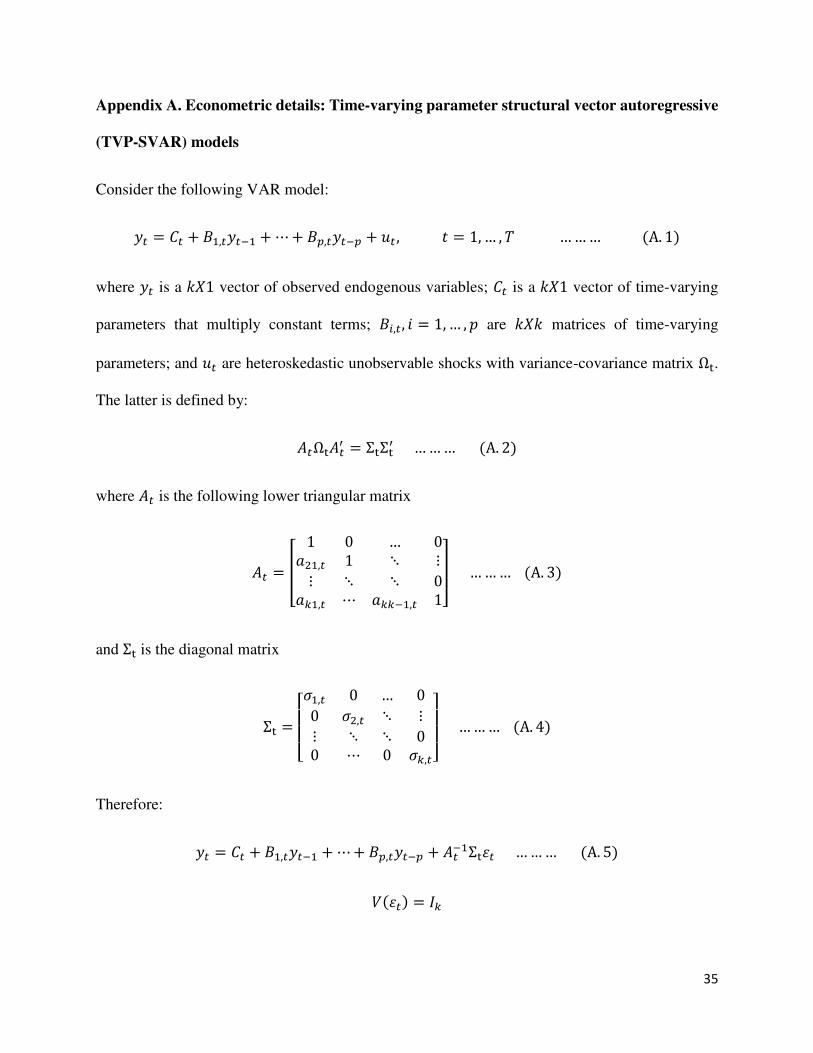
𝑦𝑡 = 𝐶𝑡 + 𝐵1,𝑡𝑦𝑡−1 + ⋯+ 𝐵𝑝,𝑡𝑦𝑡−𝑝 + 𝑢𝑡 , 𝑡 = 1,… , 𝑇 ……… (A. 1)

where 𝑦𝑡 is a 𝑘𝑋1 vector of observed endogenous variables; 𝐶𝑡 is a 𝑘𝑋1 vector of time-varying

parameters that multiply constant terms; 𝐵𝑖,𝑡, 𝑖 = 1,… , 𝑝 are 𝑘𝑋𝑘 matrices of time-varying

parameters; and 𝑢𝑡 are heteroskedastic unobservable shocks with variance-covariance matrix Ωt. The latter is defined by:

𝐴𝑡Ωt𝐴𝑡′ = ΣtΣt′ ……… (A. 2)

where 𝐴𝑡 is the following lower triangular matrix

𝐴𝑡 = [ 1 0 … 0𝑎21,𝑡 1 ⋱ ⋮⋮ ⋱ ⋱ 0𝑎𝑘1,𝑡 ⋯ 𝑎𝑘𝑘−1,𝑡 1] ……… (A. 3)

and Σt is the diagonal matrix

Σt = [ 𝜎1,𝑡 0 … 00 𝜎2,𝑡 ⋱ ⋮⋮ ⋱ ⋱ 00 ⋯ 0 𝜎𝑘,𝑡]

……… (A. 4)

Therefore:

𝑦𝑡 = 𝐶𝑡 + 𝐵1,𝑡𝑦𝑡−1 + ⋯+ 𝐵𝑝,𝑡𝑦𝑡−𝑝 + 𝐴𝑡−1Σt𝜀𝑡 ……… (A. 5)

𝑉(𝜀𝑡) = 𝐼𝑘

36

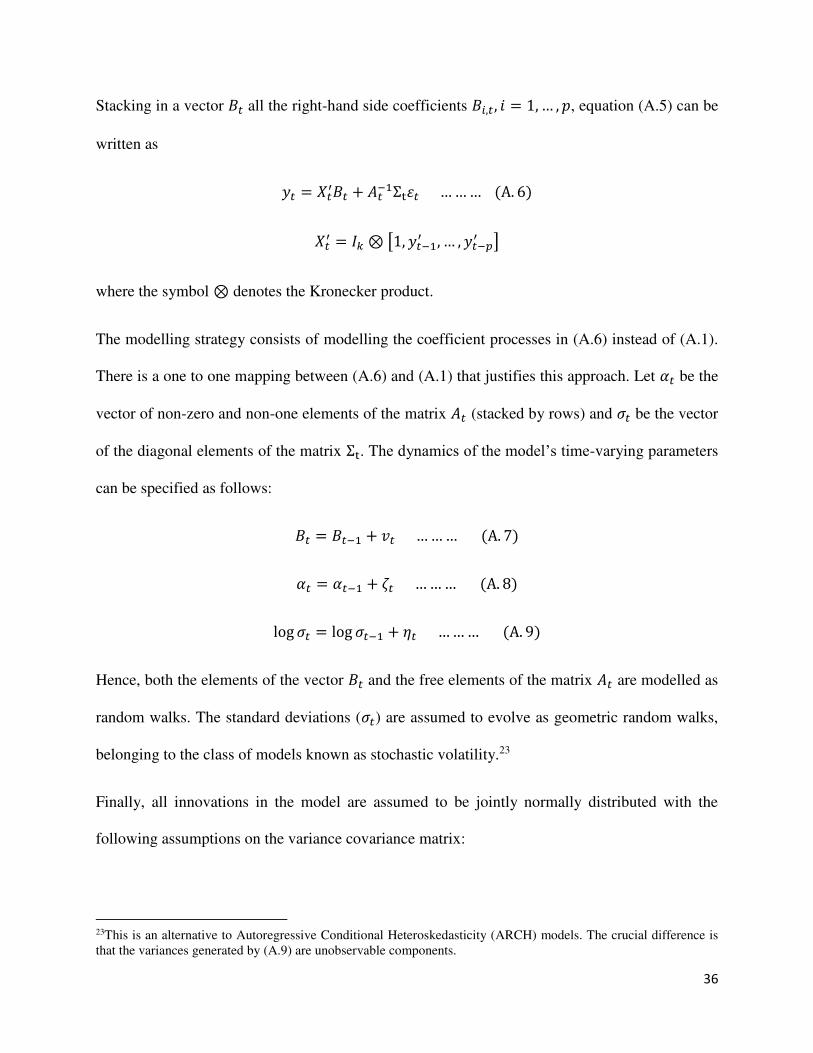
Stacking in a vector 𝐵𝑡 all the right-hand side coefficients 𝐵𝑖,𝑡, 𝑖 = 1,… , 𝑝, equation (A.5) can be

written as

𝑦𝑡 = 𝑋𝑡′𝐵𝑡 + 𝐴𝑡−1Σt𝜀𝑡 ……… (A. 6)

𝑋𝑡′ = 𝐼𝑘 ⊗ [1, 𝑦𝑡−1′ , … , 𝑦𝑡−𝑝′ ] where the symbol ⊗ denotes the Kronecker product.

The modelling strategy consists of modelling the coefficient processes in (A.6) instead of (A.1).

There is a one to one mapping between (A.6) and (A.1) that justifies this approach. Let 𝛼𝑡 be the

vector of non-zero and non-one elements of the matrix 𝐴𝑡 (stacked by rows) and 𝜎𝑡 be the vector

of the diagonal elements of the matrix Σt. The dynamics of the model’s time-varying parameters

can be specified as follows:

𝐵𝑡 = 𝐵𝑡−1 + 𝑣𝑡 ……… (A. 7)

𝛼𝑡 = 𝛼𝑡−1 + 𝜁𝑡 ……… (A. 8)

log 𝜎𝑡 = log 𝜎𝑡−1 + 𝜂𝑡 ……… (A. 9)

Hence, both the elements of the vector 𝐵𝑡 and the free elements of the matrix 𝐴𝑡 are modelled as

random walks. The standard deviations (𝜎𝑡) are assumed to evolve as geometric random walks,

belonging to the class of models known as stochastic volatility.23

Finally, all innovations in the model are assumed to be jointly normally distributed with the

following assumptions on the variance covariance matrix:

23This is an alternative to Autoregressive Conditional Heteroskedasticity (ARCH) models. The crucial difference is

that the variances generated by (A.9) are unobservable components.

37

𝑉 = ([𝜀𝑡𝑣𝑡𝜁𝑡𝜂𝑡]) = [𝐼𝑘 0 0 00 𝑄 0 00 0 𝑆 00 0 0 𝑊] ……… (A. 10)

where 𝐼𝑘 is a 𝑘-dimensional identity matrix, and 𝑄, 𝑆 and 𝑊 are positive definite matrices.

The models that depict the mass production and craft production systems were estimated following

the standard procedures outlined by Del Negro and Primiceri (2015) and Primiceri (2005). First,

we used the Gibbs sampling approach for the posterior numerical evaluation of the parameters of

interest. Second, we employed two lags for the estimation of all models. Third, the simulations

were based on 10,000 iterations of the Gibbs sample, discarding the first 2,000 for convergence.

Finally, the first 10 years (40 observations, because we used quarterly data) were used to calibrate

the prior distributions.

38

Appendix B. Complete set of results obtained from the TVP-SVAR models

.0

.1

.2

.3

.4

.5

1980 1985 1990 1995 2000 2005 2010 2015

Investment rate equation

0.0

0.4

0.8

1.2

1.6

2.0

1980 1985 1990 1995 2000 2005 2010 2015

Capacity utilization rate equation

.00

.04

.08

.12

.16

.20

.24

1980 1985 1990 1995 2000 2005 2010 2015

Employment rate equation

Figure B.1. Posterior means (blue straight lines) with 68% confidence intervals (blue dotted

lines) of the standard deviations of each equation in the TVP-SVAR model for the mass

production system (Shaded areas indicate NBER recession dates.)

39

-0.4

-0.2

0.0

0.2

0.4

0.6

0.8

1.0

2 4 6 8 10 12 14 16 18 20-.05

.00

.05

.10

.15

.20

.25

.30

.35

2 4 6 8 10 12 14 16 18 20

(a) Response of 𝑣𝑡 to an 𝑖𝑡 shock, 1977Q3 (b) Response of 𝑛𝑡 to a 𝑣𝑡 shock, 1977Q3

-0.4

-0.2

0.0

0.2

0.4

0.6

0.8

1.0

2 4 6 8 10 12 14 16 18 20-.08

-.04

.00

.04

.08

.12

.16

.20

.24

.28

.32

2 4 6 8 10 12 14 16 18 20

(c) Response of 𝑣𝑡 to an 𝑖𝑡 shock, 2004Q4 (d) Response of 𝑛𝑡 to a 𝑣𝑡 shock, 2004Q4

Figure B.2. Impulse-response functions obtained from the TVP-SVAR model that represents the

mass production system’s short-run output adjustment. Notation: 𝑣𝑡 = capacity utilization rate; 𝑖𝑡 = investment rate; and 𝑛𝑡 = employment rate. Dotted lines are the 68% confidence intervals

40

.0

.1

.2

.3

.4

.5

.6

1980 1985 1990 1995 2000 2005 2010 2015

Investment rate equation

0.0

0.4

0.8

1.2

1.6

2.0

1980 1985 1990 1995 2000 2005 2010 2015

Capacity utilization rate equation

0.0

0.2

0.4

0.6

0.8

1.0

1.2

1.4

1980 1985 1990 1995 2000 2005 2010 2015

Productivity growth equation

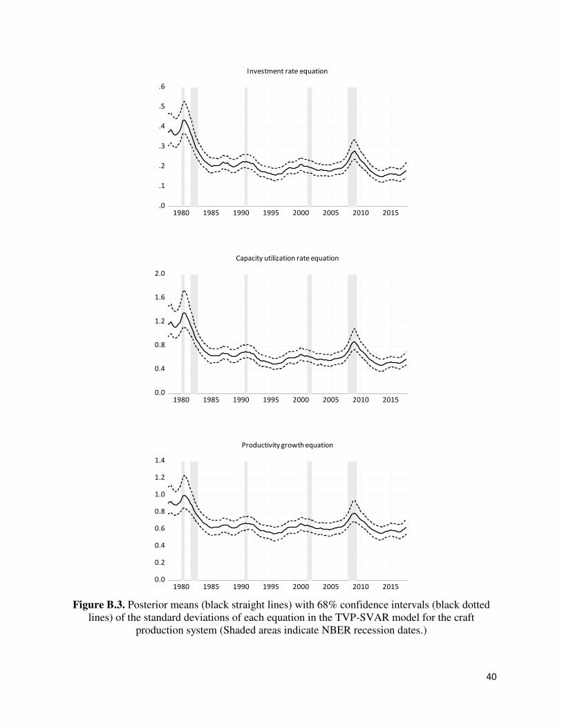
Figure B.3. Posterior means (black straight lines) with 68% confidence intervals (black dotted

lines) of the standard deviations of each equation in the TVP-SVAR model for the craft

production system (Shaded areas indicate NBER recession dates.)

41

-0.4

-0.2

0.0

0.2

0.4

0.6

0.8

1.0

2 4 6 8 10 12 14 16 18 20-.12

-.08

-.04

.00

.04

.08

.12

2 4 6 8 10 12 14 16 18 20

(a) Response of 𝑣𝑡 to an 𝑖𝑡 shock, 1978Q3 (b) Response of Δ𝜋𝑡 to an 𝑖𝑡 shock, 1978Q3

-.4

-.2

.0

.2

.4

.6

.8

2 4 6 8 10 12 14 16 18 20-.08

-.04

.00

.04

.08

.12

2 4 6 8 10 12 14 16 18 20

(c) Response of 𝑣𝑡 to an 𝑖𝑡 shock, 2004Q4 (d) Response of Δ𝜋𝑡 to an 𝑖𝑡 shock, 2004Q4

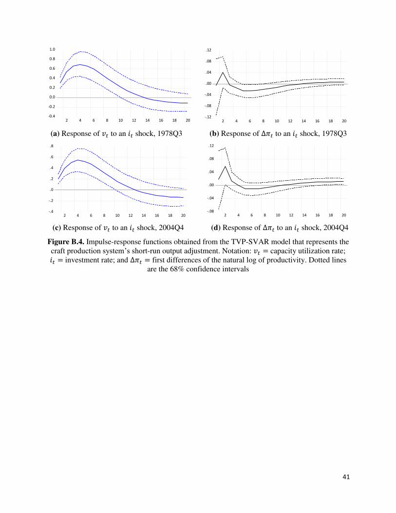
Figure B.4. Impulse-response functions obtained from the TVP-SVAR model that represents the

craft production system’s short-run output adjustment. Notation: 𝑣𝑡 = capacity utilization rate; 𝑖𝑡 = investment rate; and Δ𝜋𝑡 = first differences of the natural log of productivity. Dotted lines

are the 68% confidence intervals

Documents

The changing dynamics of short-run output adjustment