1

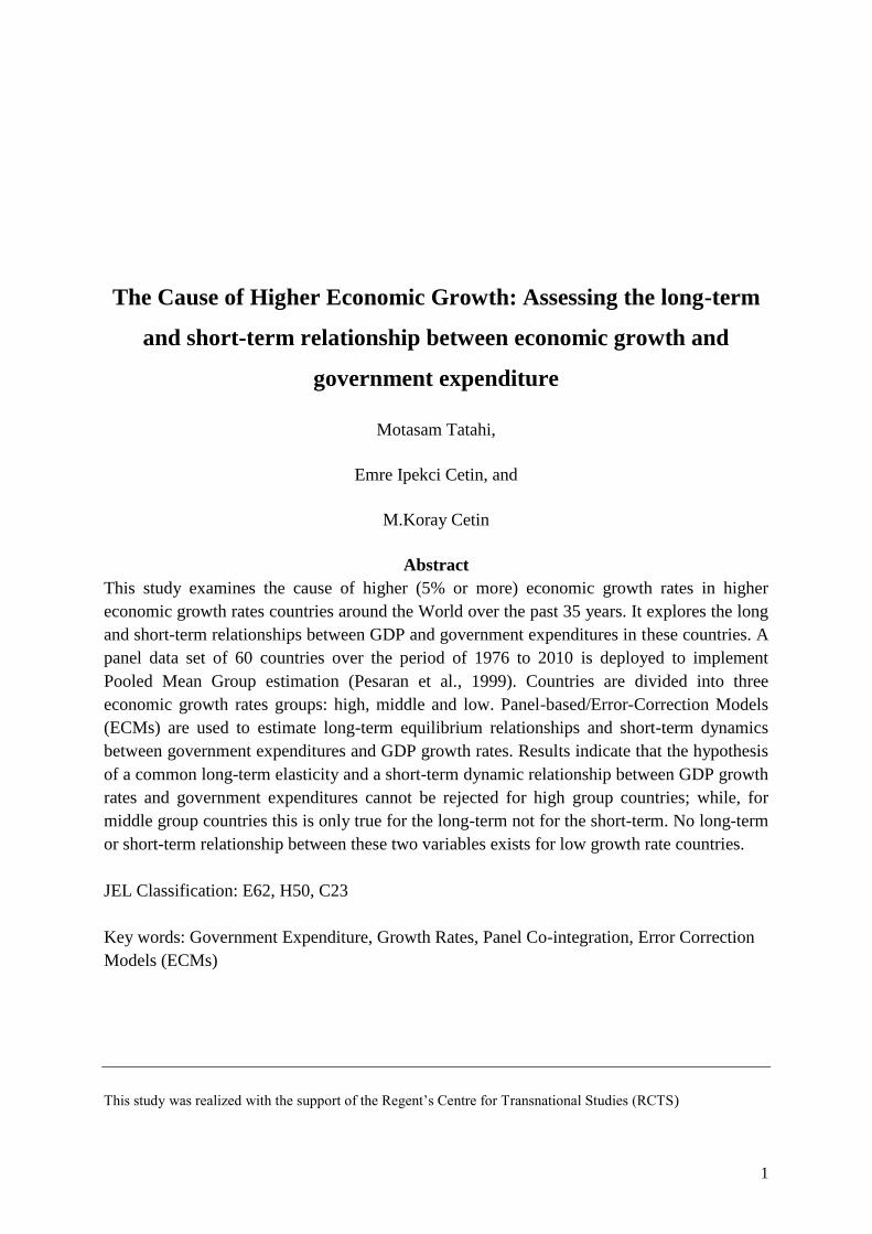
The Cause of Higher Economic Growth: Assessing the long-term

and short-term relationship between economic growth and

government expenditure

Motasam Tatahi,

Emre Ipekci Cetin, and

M.Koray Cetin

Abstract

This study examines the cause of higher (5% or more) economic growth rates in higher

economic growth rates countries around the World over the past 35 years. It explores the long

and short-term relationships between GDP and government expenditures in these countries. A

panel data set of 60 countries over the period of 1976 to 2010 is deployed to implement

Pooled Mean Group estimation (Pesaran et al., 1999). Countries are divided into three

economic growth rates groups: high, middle and low. Panel-based/Error-Correction Models

(ECMs) are used to estimate long-term equilibrium relationships and short-term dynamics

between government expenditures and GDP growth rates. Results indicate that the hypothesis

of a common long-term elasticity and a short-term dynamic relationship between GDP growth

rates and government expenditures cannot be rejected for high group countries; while, for

middle group countries this is only true for the long-term not for the short-term. No long-term

or short-term relationship between these two variables exists for low growth rate countries.

JEL Classification: E62, H50, C23

Key words: Government Expenditure, Growth Rates, Panel Co-integration, Error Correction

Models (ECMs)

This study was realized with the support of the Regent’s Centre for Transnational Studies (RCTS)

2

1. Introduction

The aim of this study is to investigate the cause of achieving higher economic growth rates

(higher than 5%) in countries with higher growth rates around the World over a period of 35

years (1976-2010). The achievement of 5 or more than 5% growth is thought to be linked to

government expenditures. I.e. high growth rates of 5 or more than 5% cannot be achieved

without higher government expenditures. To determine the cause of higher economic growth,

the links between economic growth and government expenditures are examined.

The main focus of this study lies in the dynamic properties of the relationship between these

two variables. Specifically, the aim of this study is to answer the following questions: Is

government expenditure linked to 5% or more growth output through a stable long-term

relationship? How important is the speed at which expenditure adjusts to the level of

potential output predicted in the long-run?

In two major respects, advanced knowledge of the dynamic relationship between government

expenditure and GDP need to be considered. Firstly, this knowledge improves our

understanding of long-term, structural, and public finance issues. It could, particularly, help

in assessing the impacts on expenditures and, subsequently, on deficits arising from a

structural deceleration in growth (e.g. associated with ageing populations or a decline in TFP

growth); or equally, from an improvement in growth potential (e.g. related to structural

reforms). Secondly, a more thorough understanding of the dynamic relationship between

government expenditure and GDP aids in our conception of policy-relevant issues over a

short to medium-term horizon.

It has been argued by many studies, that the key to attaining a benchmark against which to

evaluate the stance of expenditure policy and, in turn, the stance of overall fiscal policy, is to

dispose of a reliable amount of the structural relationship between government expenditure

and potential output. Understanding what neutral expenditure policy would comprise of is

necessary in order to judge whether expenditure policy is expansionary or contractionary.

However, no clear a-priori explanation exists for what expenditure policy concerns, despite a

broad consensus that a neutral revenues policy is such that government revenues move

together with output, to an extent depending on structural factors such as the degree of

progression of the tax system and the responsiveness of various tax bases with respect to

output (the output elasticity of revenues).

A benchmark for neutral expenditure policy, based on empirical evidence, can be formulated

by estimating the long-term relationship between government expenditure and GDP.

Estimates of the speed at which government expenditures adjust to GDP in the long-run,

following a shock in economic activity, would also prove useful for policy-making.

Government expenditure is assumed to be the main determinant of GDP growth. In other

words, an increase or a decrease in government expenditure is assumed to have positive or

3

negative effects on GDP growth, respectively. Three panel data sets of three group countries,

including 60 countries in total, are deployed over a period of 35 years from 1976-2010.

In this study, an attempt is made to use pure data. In particular, non-cyclical, adjusted

government expenditure and GDP data is used to determine what causes a 5% or more

growth rate. A panel dimension of this data set is utilised in a way that: (i) improves the

command of statistical tests for analysing the dynamic properties of macroeconomic series

through panel unit root and co-integration tests; and in a way that (ii) attains country-specific

information on adjustment dynamics by means of pooled mean group estimation (MPG).

We use Pooled Mean Group (PMG) estimators that allow for country-specific adjustment

coefficients in long-term panel estimation (Pesaran, Shin, and Smith (1999)). Nowadays,

PMG estimates are frequently used in applied econometric works. For example, we can point

to the analysis of institutional effects on innovation and growth (OECD (2001)); modelling

the Euro area demand of money (Golinelli and Pastorello,2002); the analysis of wealth effects

on the consumption function (Barrel and Davis, 2004); exploring the impact of policies on

fertility rates (D’Addio and Mira D’Ercole, 2005); explaining how to identify the

determinants of sovereign risks in gold standard (Cameron and Tan, 2006); analysing the link

between fiscal policies and trade balance (Funke and Nickel, 2006); and, analysing the effects

of financial intermediation on economic activity (Loayza and Ranciere, 2006).

Panel unit-root tests are performed to assess whether or not the variables we use in this

analysis are stationary. Then the existence of a long-term relationship between variables is

verified using the residual-based Pedroni (1999) panel co-integration tests. Granger (1986)

and Engle and Granger (1987) proposed models known as the Error Correction Models

(ECMs) which we found useful as a more comprehensive method of causality testing when

variables are co-integrated (Chang, 2002).The ECM model provides more information

because through its application it is possible to estimate both short and long-run effects.

According to Granger (1986), the Error-Correction Models produce better short-run forecasts

and provide the short-run dynamics necessary to obtain long-run equilibrium (Ekanayake,

1999).

The empirical analysis in the remainder of the paper proceeds as follows. After the literature

review in the second section, the methodology and data are discussed in the third section. This

is proceeding by the fourth section in which the empirical results of our analysis are presented

as follows: firstly, a description of the data set of government expenditure and potential

output is inspected by means of graphical analysis. Secondly, panel unit root tests are

performed to assess whether the variables we used in the analysis were stationary. Thirdly, the

existence of a long-term relationship between primary expenditure and potential output is

verified by means of the residual-based Pedroni (2000) panel co-integration tests. Fourthly,

the dynamic relationship between government expenditure and GDP is analysed empirically

by means of testing an error correction mechanism (ECM) with the PMG estimator.

The last section is devoted to concluding remarks.

4

2. The Literature Review

The question of whether government expenditure affects economic growth has attracted

considerable interest amongst economists and policy makers all over the world. Empirical

studies in this area seem to be moving in two directions; towards the effects of government

expenditure on economic growth, and towards how such growth can affect government

spending in the economy.

Two theoretical approaches have debated the relationship between GDP and government

expenditure. One perceived government expenditure to be an essential part of aggregate

demand in the economy, through which the fluctuation of GDP was determined. This

perception, which dominated during the 1950s and the 1960s, is now mainly referred to John

Maynard Keynes and his followers. The second theoretical approach was Wagner’s Law (a

principle named after the German economist Adolph Wagner, 1835–1917). According to

Wagner’s Law, the development of an industrial economy will be accompanied by an

increased share of public expenditure in gross national product.

In the first theoretical approach, causality runs from government spending to economic

growth, whilst in the latter law postulates that causality runs in the opposite direction (Abu-

Bader and Abu-Qarn, 2003). Following Keynes approach, public expenditure is seen as an

exogenous factor to be used as a policy instrument to influence growth. On the other hand,

Wagner argues that expenditure is an endogenous factor or an outcome, not a cause, of

growth in national income (Ansari Et al., 1997).

The relationship between government expenditure and economic growth has been tackled

from various angles by empirical literature. One angle investigates the determinants of

government size across countries, concentrating on alternative explanations such as

per-capita income (e.g., Peltzman (1980), Borcherding (1985)), the relative price of

government-provided goods and services (Baumol, 1967), demographic structures (Heller

and Diamond, 1990), and the size of (Alesina and Wacziarg ,1998) or the degree of openness

in the economy (Rodrik, 1998). Moreover, a growing strand of research aims at clarifying

cross-country structural differences in the size of government on the basis of political

fundamentals that shape the extent of deficit bias related to free-riding in government

expenditure provisions and governments’ myopia (Persson and Tabellini, 1999; Persson et

al., 2000; Milesi-Ferretti et al., 2002). It has also been shown that the way budgetary

processes are structured affects the fiscal performance of countries (e.g. Von Hagen and

Harden (1995), Hallerberg et al. (2001)).

This empirical literature also demonstrates a connection between expenditure and economic

growth over time. Some of it aims to describe long-term tendencies in history (Tanzi and

Scuckencht, 2000). Other parts of it concentrate more heavily on empirical estimations of the

elasticity of government expenditure with respect to output; often overtly aiming to

empirically test “Wagner’s Law”. For example, hypothesising that government expenditure

5

increases disproportionally to economic activity. The fundamental notion here being that,

generally, goods and services provided by the government sector - including redistribution

via transfers and the activities of public enterprises - have income elasticity greater than one,

i.e. are superior goods.

Initial analyses interpreted government expenditure as regressive to GDP without taking

dynamic properties into account (e.g., Ram, 1987). Later, test specifications were

implemented by taking non-stationarity and co-integration into account. As a result, a more

structured modelling of expenditure dynamics was enabled, introducing the distinction

between a long-term relationship and short-term adjustment (Kolluri et al., 2000; Akitoby

and Cinyabuguma, 2004; Wahab, 2004). For example, implementing cross-country analyses

allowed for dynamic specifications.

In some studies increasing government expenditure has had a positive effect on economic

growth (Singh and Sahni, 1984; Ram, 1986, Holmes and Hutton, 1990). While, in other

studies increasing government expenditure has had a negative effect on economic growth in

many developed and less-developed countries (Landau, 1983, 1986; Barth et al., 1990).

Ram (1986) found no consistent causal pattern between government expenditures and

economic growth based on his study of 63 developed and developing countries. His findings

were similar to those of Ahsan et al. (1989), which assessed US data, and those of Conte and

Darrat (1988), which analysed OECD countries’ data from 1960 to 1984. Similarly, Conte

and Darrat (1988) also found no consistent causality between the two variables.

Other studies have looked at the effect of government expenditures on economic growth using

different approaches. For example, Cheng and Lai (1997) examined the causality between

government expenditure and economic growth along with money supply using South Korean

data from1954 to 1994. In their study they found that there is bidirectional causality between

government expenditures and economic growth in South Korea.

Ghali (1999) studied the causal relationships between government expenditures and economic

growth in ten OECD countries using a quarterly data set which covered the period from

1970:1 to 1994:3. His results supported the Keynesian view.

Al-Faris (2002), examined the nature of the relationship between economic growth and public

expenditure in the Gulf Cooperation Council (GCC) using annual data from 1970 to 1997 in

the context of Wagner’s Law and Keynesian theory. This empirical investigation did not

support the hypothesis of public expenditure causing national income as proposed by

Keynesian theory.

Wahab (2004) assessed annual government expenditure and GDP time series data from 1950

to 2000 in OECD countries. He found that when the economy grows at or above trend-

growth, government expenditure tends to increase, and when economic growth slows and

6

moves to below trend-growth, growth in government expenditure declines more than

proportionately with a slowing economy.

Arpaia and Turrini (2008) estimated the long and short-run relations between government

expenditure and potential output across EU countries. They used a sample comprising of 15

EU countries over a period of 34 years (1970-2003). Their hypothesis of a common long-term

elasticity existing between cyclically-adjusted primary expenditure and potential output close

to unity could not be rejected. Despite long-run elasticity decreasing considerably over the

decades and being significantly higher than unity in catching-up countries, in fast-ageing

countries, in low-debt countries, and in countries with weak numerical rules for the control of

government spending.

Wu et al. (2010) re-examined the causal relationship between government expenditure and

economic growth in 182 countries from 1950 to 2004. Wu’s empirical results strongly

supported both Wagner’s Law and the hypothesis that government spending is helpful for

enhancing economic growth regardless of how variables are measured. When countries were

disaggregated by income levels and a degree of corruption, their results confirmed a bi-

directional causality between government activities and economic growth.

Dandan (2011) investigated the impact of public expenditures on economic growth using time

series data in Jordan from 1990 to 2006. His study found that government expenditure at the

aggregate level can have positive impacts on the growth of GDP; this being compatible with

Keynesian theory.

Ray and Ray (2012) empirically assessed the connection between government developmental

expenditure and economic growth in India using annual data from 1961-62 to 2009-10. In

their assessment, the Granger causality test confirmed the absence of any kind of short-run

causality between economic growth and developmental expenditures. Their error correction

estimates proved that developmental expenditures and GDP growth are mutually causal.

Together, these empirical studies emphasise three distinctive results. First, there is a

bidirectional causal relationship between government expenditure and economic growth.

Second, economic growth acts as a causal engine in the fluctuation of government

expenditure. Third, while causal movement from government expenditures to economic

growth is emphasised, the results of such long and short-run relationships is mixed.

3. Methodology and data

3.1. Empirical approaches

Our target is to exploit both time series and cross-sectional (i.e. across countries) data - thus,

improving the statistical properties of estimates when the number of observations over time

is based on annual data and the size of a taken sample becomes limited. When a smaller

sample size is used, this becomes a matter of consideration in the estimation and testing

7

process of stochastic properties in time series data. It may lead to low power stationarity and

co-integration tests. To avoid such outcomes, recent literature on non-stationary panel data

has concluded that inference on the time series properties of data can be improved upon

when applying integration and co-integration tests to a whole panel rather than to each unit

separately; see for instance Banerjee (1999), Baltagi and Kao (2000), Phillips and Moon

(1999a), and Smith (2000).

In order to avoid spurious regressions when time series data is deployed, the following three

steps are considered: i) we check whether or not the series are stationary; ii) we check

whether or not a co-integration relationship exists between the series when they are not

stationary, iii) when a co-integration relationship exists between series, we use Error

Correction Models (ECMs) to analyse the long-term relationship between variables jointly

with short-term adjustment towards long-term equilibrium.

3.2. Panel unit root tests

Whether or not all units are stationary with the same autoregressive coefficient across

units (the homogeneous alternative hypothesis) remains to be determined. This suggests

that in all countries, the relevant variable must congregate towards its average at the same

speed (Levin, Lin and Chu (2002) - LLC hereafter - and Breitung (2000)). It is therefore

necessary to test the null unit root hypothesis against its homogeneous alternative,

stationarity.

An Augmented Dickey-Fuller (ADF) regression of the type below should be performed for

tests which allow heterogeneous serial-correlated errors, country-specific fixed effects and

country specific deterministic trends.

∆𝑦𝑖𝑡 = 𝛿𝑖𝜏 + ∅𝑖𝑦𝑖𝑡−1 + 𝛽𝑖𝑗

𝑝𝑖

𝑗

∆𝑦𝑖𝑡−𝑗 + ∈𝑖𝑡 (1)

where yit is GDP in our case, i denotes panel units (countries in our case), t is time, τ is a

common trend across countries, pi is the country specific lag order, and ϵit are stochastic

errors.

Panel unit root tests require two conditions; one condition being cross-sectional data

independence. These tests are applied to demeaned data in order to meet this first condition.

This means that if countries are equally affected by common factors (i.e. aggregate

disturbances common to all), then demeaning the data permits one to eliminate cross-sectional

dependence. The second required condition is that data should be free of deterministic trends.

This means that if a country encounters specific deterministic trends, a unit root hypothesis

test on OLS de-trended should be performed (Phillips and Moon, 1999b). Tests are therefore

performed on demeaned and OLS de-trended data.

8

The null (H0) and alternative (H1) hypotheses are set up as follows:

𝐻0: ∅𝑖 = 0; 𝐻1: ∅𝑖 = ∅ < 0

This hypothesis testing will be carried out based on the 5% level of significance. If the

probability of the Augmented Dickey-Fuller (ADF) test is smaller than the 5% level of

significance, the null hypothesis will be rejected in favour of the alternative hypothesis.

3.3. Panel co-integration tests

The next step involves showing idiosyncratic error terms are independent across units in each

panel, i.e., conflicts in one unit do not spread to other units. However, as Banerjee et al.

(2004) noted, the existence of co-integration between some units in the panel may still exist

and there is the issue of possibly having multiple co-integration vectors.

Residual-based tests of the no co-integration null hypothesis developed by Pedroni (1995,

1997, and 1999) are employed. These tests permit country-specific short-term dynamics and

long-term relationships, and are carried out on the residuals of a static regression.

These tests are based on the following regression:

𝑒𝑖𝑡 = 𝛼𝑖 + 𝜃𝑖𝑦𝑖𝑡 + 𝑢𝑖𝑡 (2)

Where eit is the log of government expenditure, yit is the log of potential GDP in country i and

year t, uit is a stochastic residual and αi is the country specific intercept. The elasticity of

expenditure to output, θi, is allowed to vary across individual countries. The two variables are

co-integrated if the linear combination of I (1) variables is stationary. This implies that

deviations of one variable from the path prescribed by the co-integration relationship are

transitory (i.e. without memory). A long-term relationship exists between the variable in this

case, and temporary deviations can be modelled using an error correction mechanism (ECM).

Two types of tests need to be considered in order to find which one is more powerful. The

first type is called the Within Dimension Approach test. This test based on panels including:

panel v-statistic, panel p-statistic, panel PP-statistic, and panel ADF-statistic. These statistics

pool the autoregressive coefficients across different members for unit root tests on the

estimated residuals. The second test is based on the Between-Dimension Approach, which

includes group p-statistics, group PP-statistics, and group ADF-statistics. These statistics are

based on estimators that simply average the estimated coefficients for each member

individually (Lee, 2005; Apergis et al., 2010).

We restrict our analysis to panel ADF and group ADF Pedroni co-integration tests. Our

approaches are similar to the one by Pedroni (1997) for the studies of the small sample

9

properties of these tests. In terms of power, Pedroni (1997) showed that panel ADF tests (that

obtained pooling along the within dimension) perform better than other tests.

The null hypothesis of no cointegration between the series will be tested against the

alternative of they are cointegrated. The null hypothesis will be rejected in favour of the

alternative hypothesis if the probability of the ADF test is less than the level of significance of

5%.

3.4. Error Correction Models (ECMs)

The Error Correction Models (ECMs) is found plausible for this analysis. It is a

comprehensive method of causality testing when variables are co-integrated. Panel unit-root

tests and panel co-integration tests need to be performed before running the ECMs model. We

need to make sure whether or not the variables are stationary, and the existence of a long-term

relationship between variables is verified using the residual-based Pedroni (1999) method. We

follow the model proposed by Granger (1986) and Engle and Granger (1987) for the first

time.

The advantage of using an error correction specification is that, on the one hand it allows for

testing short-run relationships through lagged, differenced explanatory variables and, on the

other hand, for testing long-run relationships through lagged, error correction terms (Verma

and Arora, 2010).

A general dynamic specification can be represented by an auto-regressive distributed lag

model of order pi and qi, ARDL (pi, qi):

𝑒𝑖𝑡 = 𝜆𝑖𝑗 𝑒𝑖𝑡 .𝑗

𝑝𝑖

𝑗=1

+ 𝛿𝑖𝑗 𝑦𝑖𝑡 .𝑗

𝑞𝑖

𝑗=0

+ 𝜇𝑖 + 𝑢𝑖𝑡 (3)

where μi is an unobserved country-specific effect and uit is the error term.

The ARDL (pi, qi) can be rewritten in the following error correction model form:

Δ𝑒𝑖𝑡 = 𝜙𝑖 𝑒𝑖𝑡−1 + 𝛽𝑖

𝜙𝑖𝑦𝑖𝑡 + 𝜆𝑖𝑗

∗ Δ𝑒𝑖𝑡 .𝑗 + 𝛿𝑖𝑗∗

𝑞𝑖

𝑗=0

𝑝𝑖−1

𝑗−1

Δ𝑦𝑖𝑡 .𝑗 + 𝜇𝑖 + 𝑢𝑖𝑡 (4)

𝑤ℎ𝑒𝑟𝑒 𝜙𝑖 = − 1 − 𝜆𝑖𝑗

𝑝𝑖

𝑗=1

; 𝛽𝑖 = 𝛿𝑖𝑗

𝑞𝑖

𝑗=𝑜

; 𝜆𝑖𝑗∗ = − 𝜆𝑖𝑘 ; 𝛿𝑖𝑗

∗

𝑝𝑖

𝑘=𝑗+1

= − 𝛿𝑖𝑘

𝑝

𝑘=𝑗+1

When the ARDL (pi, qi) is stable, means error correcting, the adjustment coefficient ϕi should

be negative and less than 1 in absolute value. In this case, the long-run relationship is defined

by:

10

𝑒𝑖𝑡 = − 𝛽𝑖

′

𝜙𝑖 𝑦𝑖𝑡 + 𝜂𝑖𝑡

where ηit is a stationary process.

In the equilibrium, trend expenditure and potential output are connected to each other, with a

long-term elasticity of by

𝜃𝑖 = − 𝛽𝑖

𝜙𝑖

The ECM in equation (4) can be estimated in two different ways:

1. Traditional time series models do not take cross-country correlations in the data into

account. Dynamic fixed effect models, which control for country fixed effects, impose

the same coefficients for all countries. Unless the slope coefficients are identical,

pooling produces inconsistent estimates of the parameters value, as shown by Pesaran

and Smith (1995). In order to tackle this issue, a Mean Group estimator (MG),

consisting of estimating the coefficient of each cross-section and then taking an

average of them has been proposed by Pesaran and Smith (1995). The MG estimator,

however, does not account for the fact that some of the parameters may be the same

across countries; implying that its estimates are likely to be inefficient and strongly

affected by the presence of outliers, particularly in small samples.

2. Pesaran, Shin and Smith (1999) have proposed the Pooled Mean Group Estimator

(PMG) as an intermediate choice between imposing slope homogeneity and no

restrictions. This estimator combines the characteristics of other pooled estimators (the

fixed effect estimator in particular) with that of the mean group estimator.

Both short and long-run dynamics are treated differently by the PMG estimator. The short-

run dynamics are able to vary across countries; whereas, long-run effects must remain the

same. In the event of data having complex, country-specific, short-term dynamics that cannot

be captured, imposing the same lag structure on all countries using the PMG estimator is

appropriate. Furthermore, since it does not impose any restrictions on short-term coefficients,

the PMG provides important information on country-specific speed convergence values

which move towards the long-term relationship linking government expenditure and

potential output.

3.5. Data

Primary government expenditure is taken into account, rather than exploring the link between

economic activity and different government expenditure subcategory definitions. This broad

expenditure aggregate is employed for two reasons. Firstly, government deficit and debt, and

ultimately the overall sustainability of public finances are effectively determined by overall

government expenditure. Secondly, as found in other studies such as those of Kolluri et al.

11

(2000) and Akitoby et al. (2004), using various government expenditure categories separately

via the estimation of dynamic equations does not produce a significantly different relation to

economic activity across different types of expenditure.

In this study, business cycle adjustments have not been considered in the data of the two

variables, because the benefit of using a structural nature analysis is greater than analysing

business cycle rotations. Not considering business cycle adjustments is justifiable so long as

sample sizes are big enough.

The bottom line is that government expenditure and potential output are interconnected in

such a way that the former reacts to changes in the latter. This makes the public sector

subject to change when the size of the economy is modified. Changes in government

expenditure are presumed to affect aggregate demand, in turn changing the level of GDP. It

is still difficult to distinguish whether government expenditure affects GDP or vice-versa.

However, since this relationship is not a direct relationship and it changes through aggregate

demand, which is mostly influenced by government expenditures, at least in emerging and

developing countries, GDP, therefore, acts as a function of government expenditures (Kneller

et al., 1999; Levine and Renelt, 1992; Nijkamp and Poot, 2004).

To investigate the relationship between GDP and government expenditures, we use annual

data from 1976 to 2010 for 60 countries. Yearly observations of GDP growth rates, GDP as a

total figure and specific country government expenditures were obtained from the online

resource of the United Nations. Estimation periods were determined by the availability of

adequate data on all variables. Below are the data explanations and sources of each variable:

GDP Growth (Annual %): Annual percentage growth rates of GDP at market prices based on

constant local currency came from the EconStats web page, the World DataBank, and OECD

StatExtracts.

GDP (current US$): GDP at purchasers' prices is the sum of gross value added by all resident

producers in the economy plus any product taxes and minus any subsidies not included in the

value of the products. It is calculated without making deductions for the depreciation of

fabricated assets or for the depletion and degradation of natural resources. Data is represented

in current U.S. dollars. Dollar figures for GDP are converted from domestic currencies using

single year official exchange rates. For a few countries where the official exchange rate does

not reflect the rate effectively applied to actual foreign exchange transactions, an alternative

conversion factor is used. Data found from the EconStats web page, the World DataBank, and

OECD StatExtracts.

GEX (constant price: 2000 US$): General government final consumption expenditure

(formerly general government consumption) includes all government current expenditures for

purchases of goods and services (including compensation of employees). It also includes most

expenditure on national defence and security, but excludes government military expenditures

that are part of government capital formation. Data found from the EconStats web page, the

World DataBank, and OECD StatExtracts.

12

4. Empirical results

Countries have been split into three groups based on their annual growth rates over the

aforementioned period. The first group consists of countries having GDP annual growth rates

15 or more than 15 times bigger than 5% from 1976 to 2010. The second group consists of

countries having GDP annual growth rates 15 or more than 15 times bigger than 3% for the

same period. The last group is comprised of countries having GDP annual growth rates

smaller than 3% from 1976 to 2010. These groups are referred to as high, middle and low

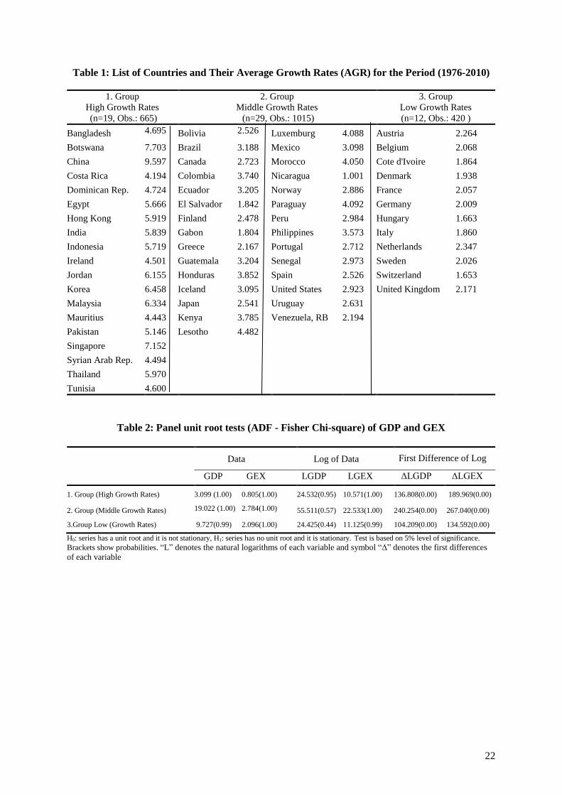
growth rate countries. As Table 1 shows, group one consists of 19 countries, group two

consists of 29 and group three of 12 countries, respectively. Table 1 gives a list of countries in

each group, as well as their average growth rates for the period from 1976 to 2010.

Put Table 1 about here

Table 1 shows that China (AGR = 9.597) was the country with the highest average growth

rate for 35 years, while Nicaragua (AGR= 1.001) was the country with the lowest average

growth rate. Though, while Nicaragua had the lowest average growth rate, it was still

included in the second group because it had a GDP annual growth rate which was at least 15

times bigger than 3% for the period from 1976 to 2010.

4.1. Graphical analysis

Prefixes L and Δ are used to indicate whether the data is in natural logarithms or in the first

difference form, respectively.

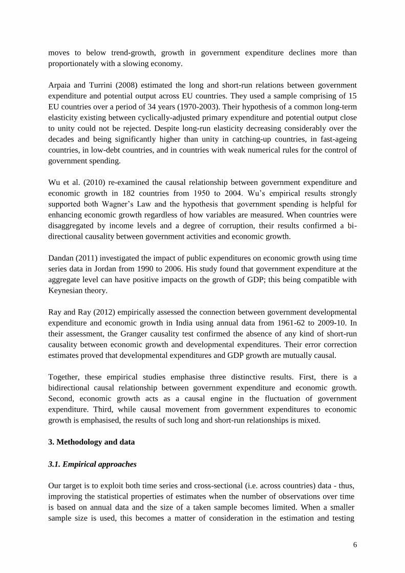
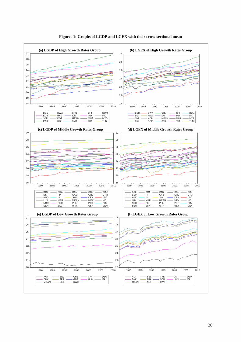
Figures 1 contain six graphs of each group’s variable based on a particular form of the natural

logarithms (L) data of GDP and GEX. All the graphs are trended and they are not stationary.

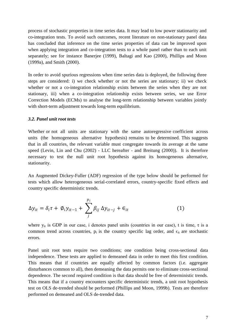
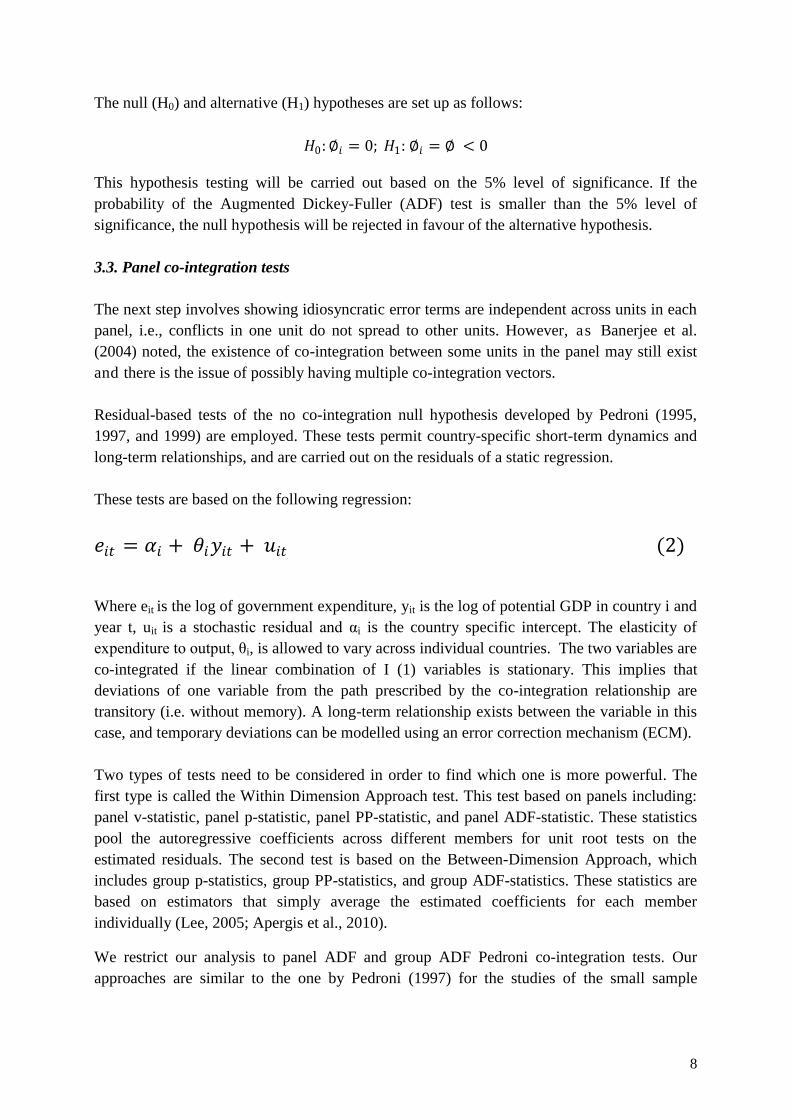
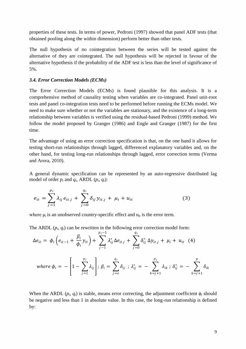
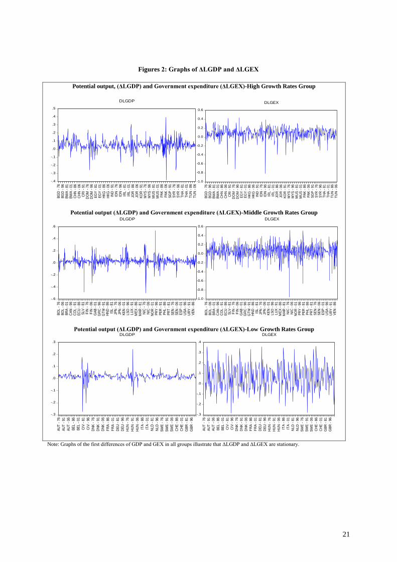
Figures 2 show graphs of two variables, ΔLGDP and ΔLGEX, in high, middle and low

growth rate countries. Graphs illustrate that first differences of GDP and GEX in all groups

are stationary because they cross the zero lines frequently.

4.2. Panel Unit Root Tests

Before implementing the short and long-run relationships between our two panel data sets of

Gross Domestic Product (GDP) and Government Expenditures (GEX), Panel Unit-Root Tests

were performed to assess whether or not the variables used in this study are stationary. The

result of the ADF tests is shown below in Table 2.

Put Table 2 about here

Probabilities of the ADF tests are presented in the brackets. Probabilities less than 0.05 means

the null hypothesis of the panel data is not stationary can be rejected in favour of the

alternative hypothesis of the panel data is stationary. The first differences of the two

13

variables’ panel data (ΔLGDP and ΔLGEX) of all groups are stationary as the probabilities

are less than the 5% significance level.

4.3. Panel Co-integration Test

The Unit Root Tests showed that the panel data sets are not stationary and they are I (1). They

will be stationary if we take the first differences of the panel data. The question that needs to

be addressed now is whether a long-term equilibrium relationship exists amongst the variables

(Chang, 2002). The existence of such a long-term relationship between Gross Domestic

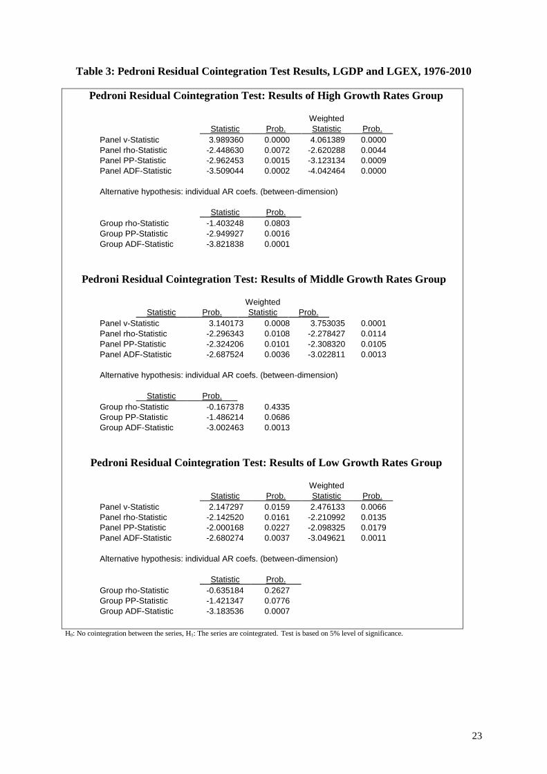
Product (GDP) and Government Expenditures (GEX) can be verified using residual-based

Pedroni (1999) Panel Co-integration Tests. These test results are reported in Table 3.

Put Table 3 about here

We conclude that primary expenditure and potential output are co-integrated on the basis of

the overall evidence, and provided that group ADF, which allows for a more general

structure of the residual correlation under the null hypothesis, is also the most effective test

(Pedroni, 1997). These results are based on the fact that the probabilities of the ADF tests are

all less than the 5% level of significance.

We proceed with modelling an error correction mechanism, which allows country-specific

and short-term coefficients, having established that government expenditure is co-

integrated with potential output.

4.4. Pooled Mean Group ECM estimation

Pooled Mean Group (PMG) estimates require disturbances to be independently distributed

across units and over time with zero mean and constant variance. We model cross-sectional

dependence assuming the existence of observable common components in the residual,

following Pesaran et al. (1999). This is captured by group, aggregate, potential output, which

is assumed to have an impact on government expenditures that will differ across countries.

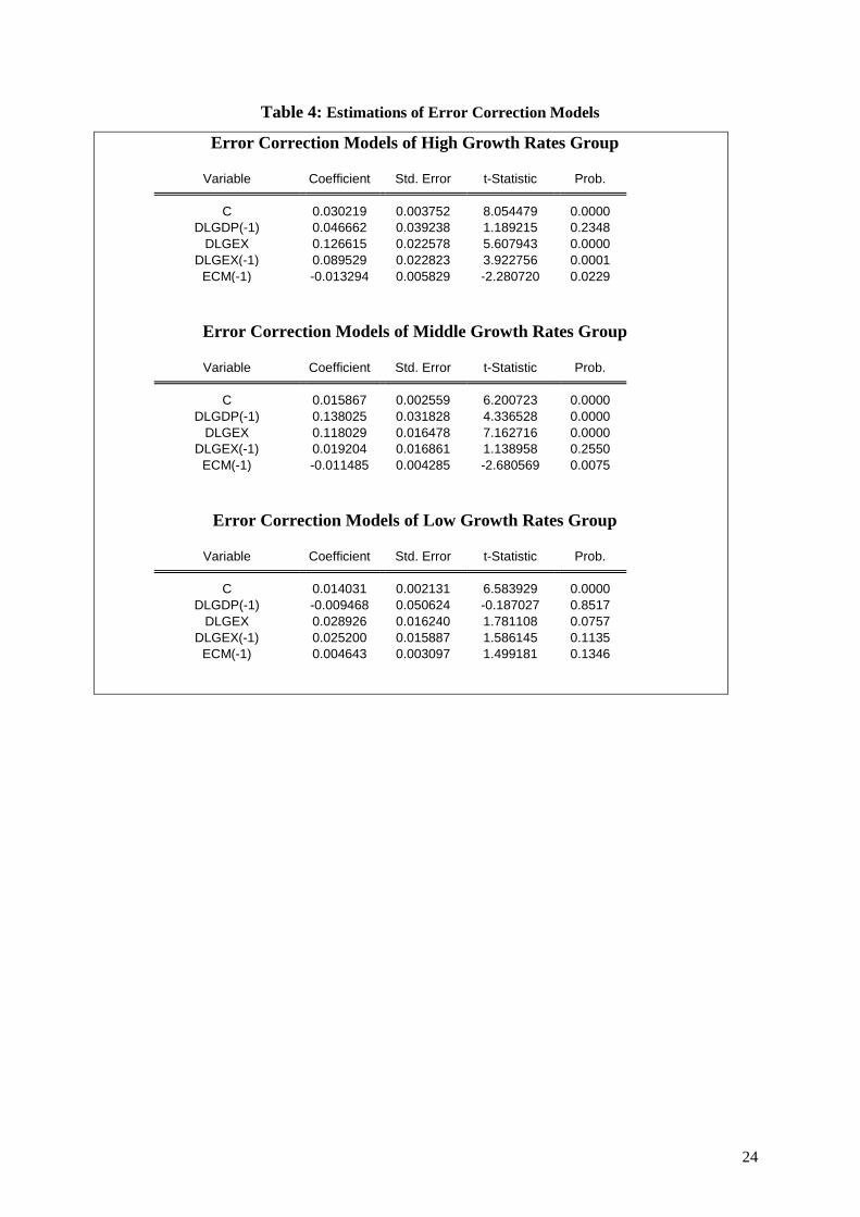
PMG estimates of the ECM are reported in Table 4.

Put Table 4 about here

The empirical evidence for the High Growth Rates Group, the result presented in the part one of

the Table 4, shows the coefficient of DLGEX (-1) is positive, 0.089529, and the obtained

probability is, 0.0001. The latter result proves that the coefficient of DLGEX (-1) is

statistically different from zero as the probability is less than the 5% level of significance. The

ECM (-1) coefficient is negative and less than one, -0.013294, and the probability of this

coefficient is, 0.0229. Since the probability is less than the 5% level of significance, the ECM

(-1) is statistically different from zero.

14

A negative and less than one error correction coefficient, and being statistically different

from zero, imply that any deviation in government expenditure from the value predicted by

the long-run relationship with potential output triggers a change in the opposite direction in

government expenditure for the high growth rates group. The average value of the error

correction coefficient of government expenditure, -0.013, implies an adjustment speed of

about less than 1 year.

From these results, it can be concluded that government expenditures have had significant

effects on GDP growth rates in the short-run as well as in the long-run in countries

experiencing high growth rates (more than 5%) for 15 or more than 15 years.

The results for the Middle Growth Rates Group, presented in the second part of the Table 4,

show the coefficient of DLGEX (-1) is positive, 0.019204, and the calculated probability is,

0.2550. The latter result proves that the coefficient of DLGEX (-1) is not statistically different

from zero as the probability is not smaller than the 5% level of significance. The ECM (-1)

coefficient is negative and less than one, -0.011485, and the probability of this coefficient is

0.0075. Since the probability is less than the 5% level of significance, the ECM (-1) is

statistically different from zero.

A negative and less than one error correction coefficient, and being statistically different

from zero, imply that any deviation in government expenditure from the value predicted by

the long-run relationship with potential output triggers a change in the opposite direction in

government expenditure for the middle growth rates group. The average value of the error

correction coefficient of government expenditure, -0.011, implies an adjustment speed of

about less than 1 year.

From these results, it can be concluded that government expenditures have had significant

effects on GDP growth rates in the long-run only, not having any affects in the short-run in

countries experiencing middle growth rates (more than 3%) for 15 or more than 15 years.

The results for Low Growth Rates Group, as it is shown in the third part of the Table 4, display

the coefficient of DLGEX (-1) is positive, 0.025200, and the calculated probability is, 0.1135.

The latter result proves that the coefficient of DLGEX (-1) is not statistically different from

zero since the probability is not smaller than the 5% level of significance. The ECM (-1)

coefficient is not negative but it is less than one, 0.004643. The probability of this coefficient

is 0.1346. Since the probability is not less than the 5% level of significance, the ECM (-1) is

not statistically different from zero.

From these results, it can be concluded that government expenditures have not had significant

effects on GDP growth rates in the long-run only as well as in the short-run in countries

experiencing low growth rates (less than 3%) for 15 or more than 15 years.

These results imply explicitly that without high government expenditures higher than 5%

15

economic growth rates cannot be achieved in the short-run as well as in the long-run.

Furthermore, the results found verify that the low economic growth rate links with low

government expenditures. High government expenditures are essential for high economic

growth rates.

5. Concluding remarks

An estimation of the long and short-term relations between government expenditure and

potential output for high, middle and low growth rate countries around the world has been

given throughout this paper. The aim of this study was to determine what causes 5% or more

economic growth over time and across countries.

Estimating a dynamic relationship between the two variables turns out to be possible

using the Pooled Mean Group (PMG) estimator (Pesaran, Shin, and Smith (1999)). This

procedure allows one to combine the accuracy of estimates by pooling data from cross-

country dimensions; while, at the same time, limiting the risk of estimate inconsistencies

associated with the possible heterogeneity of regression coefficients across countries. The

PMG enacts a common long-term elasticity for all countries, while allowing for country-

specific short-term elasticities.

Results show that the assumption of a common long-run elasticity is the case for the data of

all country groups and is below unity. Group country-specific short-term elasticities imply

on average a speed of adjustment of government expenditure to potential output of about

1 year.

This study assumed that government expenditure is the main determinant of high economic

growth. Panel co-integration tests revealed that government expenditure and potential

output in high growth rate countries are linked by a stable long-term relationship.

For middle growth rate countries, the long-run relationship between government expenditure

and potential output was found to be statistically significant; while, the short-run relationship

was found to be statistically insignificant.

For low economic growth rate countries neither long-run nor short-run relationship between

government expenditure and potential output were found to be statistically significant.

What is found shows explicitly that high economic growth achievement is severely linked to

government expenditure. Governments of countries that reached at least 15 times economic

growth rates of 5% or more have spent more than countries that have achieved 3-5%

economic growth rates, called ‘middle growth rate countries’, and less than 3% economic

growth rates, called ‘low growth rate countries’.

As economic growth theories and empirical studies have established, economic growth is

linked to many economic factors, such as aggregate demand in the short-run, factors of

production in between, and factors like education and government economic policy in the

16

long-run. However, as this study shows, the achievement of higher than 5% economic growth

rates is tied to government expenditures.

References

Abu-Bader S. and Abu-Qarn A.S., (2003), “Government Expenditures, Military Spending and

Economic Growth: Causality Evidence from Egypt, Israel, and Syria”, Journal of Policy Modelling,

25, 567–583.

Ahsan S., Kwan A. and Sahni B., (1989), “Causality between Government Consumption Expenditures

and National Income: OECD Countries”, Public Finance, 44(2), pp. 204-224.

Akitoby, B. and Cinyabuguma, M., (2004), “Sources of growth in the Democratic Republic of the

Congo: a Cointegration Approach”, IMF working paper, 04/114. Washington DC: International

monetary fund.

Alesina, A., and R. Wacziarg, (1998), “Openness, Country Size, and Government”, Journal of Public

Economics, 49, 305-21.

Al-Faris A.F., (2002), “Public Expenditure and Economic Growth in the Gulf Cooperation Council

Countries”, Applied Economics, 34(9), 1187-1193.

Ansari M.I., Gordon D.V. and Akuamoah C., (1997), “Keynes versus Wagner: Public Expenditure and

National Income for Three African Countries”, Applied Economics, 29, 543-550.

Apergis N., Dincer O.C. and Payne J.E., (2010), “The Relationship between Corruption and Income

Inequality in U.S. States: Evidence from a Panel Cointegration and Error Correction Model”, Public

Choice, 145, 125–135.

Arpaia A and Turrini A., (2008), “Government Expenditure and Economic Growth in the EU: Long-

run Tendencies and Short-term Adjustment, European Economy”, Economic Papers 300, Directorate

General Economic and Monetary Affairs, European Commission.

Baltagi, B. H. and Kao, C., (2000), “Non Stationary Panels, Cointegration in Panels, and Dynamic

Panels: a Survey” in B. Baltagi (ed.), Advances in Econometrics, Vol. 15: Non-stationary Panels,

Panel Cointegration, and Dynamic Panels, Amsterdam: JAI Press

Banerjee, A., (1999), “Panel Unit Roots and Cointegration: an Overview” Oxford Bulletin of

Economics and Statistics, Special Issue.

Banerjee, A., Marcellino, M. and Osbat C., (2004), “Some Cautions on the Use of Panel Methods for

Integrated Series of Macroeconomic Data” Econometrics Journal, 7, 322-340.

Barrell, R. and Davis E.P., (2004), “Consumption, Financial and Real Wealth in the G-5”, Discussion

Paper No. 232, National Institute of Economic and Social Research, London.

Barth, J., Keleher, R., and Russek, F., (1990), “The Scale of Government and Economic Activity”,

The Southern Business and Economic Journal, 142-83.

Baumol, W. (1967), “Macroeconomics of Unbalanced Growth: The Anatomy of Urban Crisis”,

American Economic Review, vol. 57, pp. 415-426.

Borcherding, T.E., (1985), “The Causes of Government Expenditure Growth: a Survey of the US

Evidence”, Journal of Public Economics, vol. 28, pp. 359-382.

17

Breitung, J., (2000), “The Local Power of Some Unit Root Tests for Panel Data,” in B. Baltagi (ed.),

Advances in Econometrics, Vol. 15: Non-stationary Panels, Panel Cointegration, and Dynamic Panels,

Amsterdam: JAI Press, p. 161–178.

Cameron G., Gai P. and Tan K. Y., (2006), “Sovereign Risk in the Classical Gold Standard Era”,

Working Paper 11, Australian National University - Centre for Applied Macroeconomic Analysis.

Chang, T., (2002), “An Econometric Test for Wagner's Law for Six Countries Based on Cointegration

and Error Correction Modelling Techniques”, Applied Economics, 34, 1157-1169.

Cheng B.S., Lai T.W., (1997), “Government Expenditures and Economic Growth in South Korea: A

VAR Approach”, Journal of Economic Development, 22(1), 11-24.

Conte M. A., Darrat A.F., (1988), “Economic Growth and the Expanding Public Sector: A Re-

examination”, The Review of Economics and Statistics, 70(2), 322-330.

D’Addio, A., and Mira D’Ercole, M., (2005), “Policies, Institutions and Fertility Rates: A Panel Data

Analysis in OECD Countries”, OECD Economic Studies, 41.

Dandan M.M., (2011), “Government Expenditures and Economic Growth in Jordan”, International

Conference on Economics and Finance Research (IPEDR), Vol.4, 467-470, IACSIT Press, Singapore.

Ekanayake E.M., (1999), “Exports and Economic Growth in Asian Developing Countries:

Cointegration and Error-Correction Models”, Journal of Economic Development, 24(2), 43-56.

Engle, R. F., and Granger C. W. J., (1987), “Cointegration and Error Correction: Representation,

Estimation, and Testing”, Econometrica, 55, 251-76.

Funke, K. and Nickel, C., (2006), “Does fiscal policy matter for the trade account? A panel

Cointegration Study”, ECB Working Paper, 620.

Ghali K.H., (1999), “Government Size and Economic Growth: Evidence from a Multivariate

Cointegration Analysis”, Applied Economics, 31(8), 975-987.

Golinelli, R. and Pastorello S., (2002,) “Modelling the Demand for M3 in the Euro Area”, The

European Journal of Finance, 8, 371-401

Granger, C.W.J., (1986), “Developments in the Study of Cointegrated Economic Variables”, Oxford

Bulletin of Economics and Statistics, 48, 213-228.

Guellec, D. and B. van Pottelsberghe de la Potterie. (2001), “R&D and Productivity Growth: Panel

Data Analysis of 16 OECD Countries”, OECD Economic Studies, No. 33, 2001/II.

Halleberg, M., Strauch, R. and Von Hagen, J., (2001), “The Use and Effectiveness of Budgetary Rules

and Norms in EU Member States”, Report prepared for the Dutch Ministry of Finance by the Institute

of European Integration Studies.

Heller, P. S., and Diamond J., (1990), “International Comparison of Government Expenditure

Revisited: the Developing Countries 1975-1986”, IMF Occasional Paper, 69.

Holmes, J. M. and Hutton P.A., (1990), “On the Causal Relationship between Government

Expenditures and National Income”, The Review of Economics and Statistics, 72(1), pp. 87-95.

18

Kneller, R., Bleaney M. F. and Gemmell N., (2004), “Fiscal Policy and Growth: Evidence from

OECD Countries”, Journal of Public Economics, 74, 171-190.

Kolluri, B.R., Panik M. J. and Wahab M.S., (2000), “Government Expenditure and Economic Growth:

Evidence from G7 Countries”, Applied Economics, 32, 1059-1068.

Landau D., (1983), “Government Expenditure and Economic Growth: A Cross-Country Study”,

Southern Economic Journal, 49(3), 783-792.

Landau D., (1986), “Government and Economic Growth in the Less Developed Countries: An

Empirical Study for 1960-1980”, Economic Development and Cultural Change, 35(1), 35-75.

Lee C.C., (2005), “Energy Consumption and GDP in Developing Countries: A Cointegrated Panel

Analysis”, Energy Economics, 27, 415– 427.

Levin A., Lin, C.-F. and Chu C.-S.J., (2002), “Unit Roots Tests in panel Data: Asymptotics and Finite

Sample Properties”, Journal of Econometrics, 108, 1-24.

Levine, R., and D. Renelt, (1992), “A Sensitivity Analysis of Cross-Country Growth Regressions”,

American Economic Review, 82, 942-963.

Loayza, N. and Ranciere, R., (2006), “Financial Development, Financial Fragility, and Growth”

Journal of Money, Credit, and Banking, 38,.1051-1076.

Milesi Ferretti, G.M., Perotti R. and Rostagno M., (2002), “Electoral Systems and Public Spending”,

Quarterly Journal of Economics, 117, 609-656.

Nijkamp, P., and Poot J., (2004), “Meta-analysis of the Effect of Fiscal Policy on Long-run

Growth”, European Journal of European Economy, 20, 91, 124.

Pedroni, P., (1995), “Panel Cointegration; Asymptotic and Finite Sample Properties of Pooled Time

Series Tests, with an Application to the PPP Hypothesis”, Indiana University working papers in

economics, 95-013

Pedroni, P., (1997), “On the Role of Cross Sectional Dependency in Panel Unit Root and Panel

Cointegration Exchange Rate Studies”, Working paper, Indiana University.

Pedroni, P., (1999), “Critical Values for Cointegration Tests in Heterogeneous Panels with Multiple

Regressors”, Oxford Bulletin of Economics and Statistics, 61(S1), 653-670.

Peltzman, S.^, (1980), “The Growth of Government”, The Journal of Law and Economics, 23, 209–

289.

Persson, T., and Tabellini G., (1999), “The Size and Scope of Government: Comparative Policies with

Rational Politicians”, European Economic Review, 63, 699-735.

Perotti, R., (2002), “Estimating the Effects of Fiscal Policy in OECD countries”, ECB Working Paper,

168.

Persson, T., Roland G. and Tabellini G., (2000), “Comparative Politics and Public Finance.” Journal

of Political Economy, 108, 1121-1161.

Pesaran, M. H. and Smith, R., (1995), “Estimating Long-run Relationship from Dynamic

Heterogeneous Panel”, Journal of Econometrics, 68, 79-113.

19

Pesaran, M. H., Shin, Y. and Smith, R., (1999), “Pooled Mean Group Estimator of Dynamic

Heterogeneous Panels”, Journal of the American Statistical Association, Vol 94 pp.621-634.

Phillips, P.C.B. and Moon, H. R., (1999a), “Non-stationary Panel Data Analysis: An Overview of

Some Recent Developments”, Cowles Foundation Discussion Papers, 1221, Cowles Foundation, Yale

University.

Phillips, P.C.B. and Moon, H. R., (1999b), “Linear Regression Limit Theory for Non-stationary Panel

Data”, Econometrica, 67, 1057-1112.

Ram R., (1986), “Government Size and Economic Growth: A New Framework and Some Evidence

from Cross-Section and Time-Series Data”, American Economic Review, 76(1), 191-203.

Ram, R., (1987), “Wagner’s Hypothesis in Time-Series and Cross-Section Perspectives: Evidence

from ‘Real’ Data for 115 Countries”, Review of Economics and Statistics, 69, 194-204.

Ray S. and Ray I.A., (2012), “On the Relationship between Government’s Developmental Expenditure

and Economic Growth in India: A Cointegration Analysis”, Advances in Applied Economics and

Finance, 1(2), 86- 94.

Rodrik, D., (1998), “Why do more open economies have bigger governments?”, Journal of Political

Economy, 151, 997-1032.

Singh B. and Sahni B.S., (1984), “Causality between Public Expenditure and National Income”, The

Review of Economics and Statistics, 66(4), 630-644.

Smith R.P., (2000), “Estimation and Inference with Non-Stationary Panel Time-Series Data”,

Department of Economics, Birbeck College, London.

Tanzi, V. and Schuknecht L., (2000), Public Spending in the 20th Century: A Global Perspective,

Cambridge University Press, Cambridge.

Von Hagen J. and Harden I.J., (1995), “Budget Processes and Commitment to Fiscal Discipline”,

European Economic Review, 39(3), 771-779.

Verma S. and Arora R., (2010), “Does the Indian Economy Support Wagner’s Law? An Econometric

Analysis”, Eurasian Journal of Business and Economics, 3 (5), 77-91.

Wahab, M., (2004) “Economic Growth and Government Expenditure: Evidence from a New Test

Specification”, Applied Economics, 36, 2125-2135.

Wu S.Y., Tang J.H., Lin E.S., (2010), “The Impact of Government Expenditure on Economic

Growth: How Sensitive to the Level of Development?”, Journal of Policy Modelling, 32, 804–817.

20

Figures 1: Graphs of LGDP and LGEX with their cross-sectional mean

(a) LGDP of High Growth Rates Group (b) LGEX of High Growth Rates Group

18

20

22

24

26

28

30

1980 1985 1990 1995 2000 2005 2010

BGD BWA CHN CRI DOMEGY HKG IDN IND IRL

JOR KOR MEAN MUS MYS

PAK SGP SYR THA TUN

(c) LGDP of Middle Growth Rates Group (d) LGEX of Middle Growth Rates Group

16

18

20

22

24

26

28

30

1980 1985 1990 1995 2000 2005 2010

BOL BRA CAN COL ECUESP FIN GAB GRC GTM

HND ISL JPN KEN LSO

LUX MAR MEAN MEX NIC

NOR PER PHL PRT PRY

SEN SLV URY USA VEN

18

20

22

24

26

28

30

32

1980 1985 1990 1995 2000 2005 2010

BOL BRA CAN COL ECUESP FIN GAB GRC GTM

HIND ISL JPN KEN LSO

LUX MAR MEAN MEX NIC

NOR PER PHL PRT PRY

SEN SLV URY USA VEN

(e) LGDP of Low Growth Rates Group (f) LGEX of Low Growth Rates Group

20

21

22

23

24

25

26

27

1980 1985 1990 1995 2000 2005 2010

AUT BEL CHE CIV DEU

DNK FRA GBR HUN ITA

MEAN NLD SWE

22

23

24

25

26

27

28

29

1980 1985 1990 1995 2000 2005 2010

AUT BEL CHE CIV DEU

DNK FRA GBR HUN ITA

MEAN NLD SWE

18

19

20

21

22

23

24

25

26

27

1980 1985 1990 1995 2000 2005 2010

BGD BWA CHN CRI DOMEGY HKG IDN IND IRL

JOR KOR MEAN MUS MYS

PAK SGP SYR THA TUN

21

Figures 2: Graphs of ΔLGDP and ΔLGEX

Potential output, (ΔLGDP) and Government expenditure (ΔLGEX)-High Growth Rates Group

-.4

-.3

-.2

-.1

.0

.1

.2

.3

.4

.5

BG

D -

76

BG

D -

96

BW

A -

81

BW

A -

01

CH

N -

86

CH

N -

06

CR

I -

91

DO

M -

76

DO

M -

96

EG

Y -

81

EG

Y -

01

HK

G -

86

HK

G -

06

IND

- 9

1ID

N -

76

IDN

- 9

6IR

L -

81

IRL -

01

JOR

- 8

6JO

R -

06

KO

R -

91

MY

S -

76

MY

S -

96

MU

S -

81

MU

S -

01

PA

K -

86

PA

K -

06

SG

P -

91

SY

R -

76

SY

R -

96

TH

A -

81

TH

A -

01

TU

N -

86

TU

N -

06

DLGDP

-1.0

-0.8

-0.6

-0.4

-0.2

0.0

0.2

0.4

0.6

BG

D -

76

BG

D -

96

BW

A -

81

BW

A -

01

CH

N -

86

CH

N -

06

CR

I -

91

DO

M -

76

DO

M -

96

EG

Y -

81

EG

Y -

01

HK

G -

86

HK

G -

06

IND

- 9

1ID

N -

76

IDN

- 9

6IR

L -

81

IRL -

01

JOR

- 8

6JO

R -

06

KO

R -

91

MY

S -

76

MY

S -

96

MU

S -

81

MU

S -

01

PA

K -

86

PA

K -

06

SG

P -

91

SY

R -

76

SY

R -

96

TH

A -

81

TH

A -

01

TU

N -

86

TU

N -

06

DLGEX

Potential output (ΔLGDP) and Government expenditure (ΔLGEX)-Middle Growth Rates Group

-.6

-.4

-.2

.0

.2

.4

.6

BO

L -

76

BO

L -

06

BR

A -

01

CA

N -

96

CO

L -

91

EC

U -

86

SL

V -

81

FIN

- 7

6F

IN -

06

GA

B -

01

GR

C -

96

GT

M -

91

HN

D -

86

ISL

- 8

1JP

N -

76

JPN

- 0

6K

EN

- 0

1L

SO

- 9

6L

UX

- 9

1M

EX

- 8

6M

AR

- 8

1N

IC -

76

NIC

- 0

6N

OR

- 0

1P

RY

- 9

6P

ER

- 9

1P

HL -

86

PR

T -

81

SE

N -

76

SE

N -

06

ES

P -

01

US

A -

96

UR

Y -

91

VE

N -

86

DLGDP

-1.0

-0.8

-0.6

-0.4

-0.2

0.0

0.2

0.4

0.6

BO

L -

76

BO

L -

06

BR

A -

01

CA

N -

96

CO

L -

91

EC

U -

86

SL

V -

81

FIN

- 7

6F

IN -

06

GA

B -

01

GR

C -

96

GT

M -

91

HN

D -

86

ISL

- 8

1JP

N -

76

JPN

- 0

6K

EN

- 0

1L

SO

- 9

6L

UX

- 9

1M

EX

- 8

6M

AR

- 8

1N

IC -

76

NIC

- 0

6N

OR

- 0

1P

RY

- 9

6P

ER

- 9

1P

HL -

86

PR

T -

81

SE

N -

76

SE

N -

06

ES

P -

01

US

A -

96

UR

Y -

91

VE

N -

86

DLGEX

Potential output (ΔLGDP) and Government expenditure (ΔLGEX)-Low Growth Rates Group

-.3

-.2

-.1

.0

.1

.2

.3

AU

T -

76

AU

T -

91

AU

T -

06

BE

L -

86

BE

L -

01

CIV

- 8

1

CIV

- 9

6

DN

K -

76

DN

K -

91

DN

K -

06

FR

A -

86

FR

A -

01

DE

U -

81

DE

U -

96

HU

N -

76

HU

N -

91

HU

N -

06

ITA

- 8

6

ITA

- 0

1

NLD

- 8

1

NLD

- 9

6

SW

E -

76

SW

E -

91

SW

E -

06

CH

E -

86

CH

E -

01

GB

R -

81

GB

R -

96

DLGDP

-.3

-.2

-.1

.0

.1

.2

.3

.4

AU

T -

76

AU

T -

91

AU

T -

06

BE

L -

86

BE

L -

01

CIV

- 8

1

CIV

- 9

6

DN

K -

76

DN

K -

91

DN

K -

06

FR

A -

86

FR

A -

01

DE

U -

81

DE

U -

96

HU

N -

76

HU

N -

91

HU

N -

06

ITA

- 8

6

ITA

- 0

1

NLD

- 8

1

NLD

- 9

6

SW

E -

76

SW

E -

91

SW

E -

06

CH

E -

86

CH

E -

01

GB

R -

81

GB

R -

96

DLGEX

Note: Graphs of the first differences of GDP and GEX in all groups illustrate that ΔLGDP and ΔLGEX are stationary.

22

Table 1: List of Countries and Their Average Growth Rates (AGR) for the Period (1976-2010)

1. Group

High Growth Rates

(n=19, Obs.: 665)

2. Group

Middle Growth Rates

(n=29, Obs.: 1015)

3. Group

Low Growth Rates

(n=12, Obs.: 420 )

Bangladesh 4.695 Bolivia 2.526 Luxemburg 4.088 Austria 2.264

Botswana 7.703 Brazil 3.188 Mexico 3.098 Belgium 2.068

China 9.597 Canada 2.723 Morocco 4.050 Cote d'Ivoire 1.864

Costa Rica 4.194 Colombia 3.740 Nicaragua 1.001 Denmark 1.938

Dominican Rep. 4.724 Ecuador 3.205 Norway 2.886 France 2.057

Egypt 5.666 El Salvador 1.842 Paraguay 4.092 Germany 2.009

Hong Kong 5.919 Finland 2.478 Peru 2.984 Hungary 1.663

India 5.839 Gabon 1.804 Philippines 3.573 Italy 1.860

Indonesia 5.719 Greece 2.167 Portugal 2.712 Netherlands 2.347

Ireland 4.501 Guatemala 3.204 Senegal 2.973 Sweden 2.026

Jordan 6.155 Honduras 3.852 Spain 2.526 Switzerland 1.653

Korea 6.458 Iceland 3.095 United States 2.923 United Kingdom 2.171

Malaysia 6.334 Japan 2.541 Uruguay 2.631

Mauritius 4.443 Kenya 3.785 Venezuela, RB 2.194

Pakistan 5.146 Lesotho 4.482

Singapore 7.152

Syrian Arab Rep. 4.494

Thailand 5.970

Tunisia 4.600

Table 2: Panel unit root tests (ADF - Fisher Chi-square) of GDP and GEX

Data Log of Data First Difference of Log

GDP GEX LGDP LGEX ΔLGDP ΔLGEX

1. Group (High Growth Rates) 3.099 (1.00) 0.805(1.00) 24.532(0.95) 10.571(1.00) 136.808(0.00) 189.969(0.00)

2. Group (Middle Growth Rates) 19.022 (1.00) 2.784(1.00) 55.511(0.57) 22.533(1.00) 240.254(0.00) 267.040(0.00)

3.Group Low (Growth Rates) 9.727(0.99) 2.096(1.00) 24.425(0.44) 11.125(0.99) 104.209(0.00) 134.592(0.00)

H0: series has a unit root and it is not stationary, H1: series has no unit root and it is stationary. Test is based on 5% level of significance.

Brackets show probabilities. “L” denotes the natural logarithms of each variable and symbol “Δ” denotes the first differences

of each variable

23

Table 3: Pedroni Residual Cointegration Test Results, LGDP and LGEX, 1976-2010

Pedroni Residual Cointegration Test: Results of High Growth Rates Group

Weighted

Statistic Prob. Statistic Prob.

Panel v-Statistic 3.989360 0.0000 4.061389 0.0000

Panel rho-Statistic -2.448630 0.0072 -2.620288 0.0044

Panel PP-Statistic -2.962453 0.0015 -3.123134 0.0009

Panel ADF-Statistic -3.509044 0.0002 -4.042464 0.0000

Alternative hypothesis: individual AR coefs. (between-dimension)

Statistic Prob.

Group rho-Statistic -1.403248 0.0803

Group PP-Statistic -2.949927 0.0016

Group ADF-Statistic -3.821838 0.0001

Pedroni Residual Cointegration Test: Results of Middle Growth Rates Group

Weighted

Statistic Prob. Statistic Prob.

Panel v-Statistic 3.140173 0.0008 3.753035 0.0001

Panel rho-Statistic -2.296343 0.0108 -2.278427 0.0114

Panel PP-Statistic -2.324206 0.0101 -2.308320 0.0105

Panel ADF-Statistic -2.687524 0.0036 -3.022811 0.0013

Alternative hypothesis: individual AR coefs. (between-dimension)

Statistic Prob.

Group rho-Statistic -0.167378 0.4335

Group PP-Statistic -1.486214 0.0686

Group ADF-Statistic -3.002463 0.0013

Pedroni Residual Cointegration Test: Results of Low Growth Rates Group

Weighted

Statistic Prob. Statistic Prob.

Panel v-Statistic 2.147297 0.0159 2.476133 0.0066

Panel rho-Statistic -2.142520 0.0161 -2.210992 0.0135

Panel PP-Statistic -2.000168 0.0227 -2.098325 0.0179

Panel ADF-Statistic -2.680274 0.0037 -3.049621 0.0011

Alternative hypothesis: individual AR coefs. (between-dimension)

Statistic Prob.

Group rho-Statistic -0.635184 0.2627

Group PP-Statistic -1.421347 0.0776

Group ADF-Statistic -3.183536 0.0007

H0: No cointegration between the series, H1: The series are cointegrated. Test is based on 5% level of significance.

24

Table 4: Estimations of Error Correction Models

Error Correction Models of High Growth Rates Group

Variable Coefficient Std. Error t-Statistic Prob. C 0.030219 0.003752 8.054479 0.0000

DLGDP(-1) 0.046662 0.039238 1.189215 0.2348

DLGEX 0.126615 0.022578 5.607943 0.0000

DLGEX(-1) 0.089529 0.022823 3.922756 0.0001

ECM(-1) -0.013294 0.005829 -2.280720 0.0229

Error Correction Models of Middle Growth Rates Group

Variable Coefficient Std. Error t-Statistic Prob. C 0.015867 0.002559 6.200723 0.0000

DLGDP(-1) 0.138025 0.031828 4.336528 0.0000

DLGEX 0.118029 0.016478 7.162716 0.0000

DLGEX(-1) 0.019204 0.016861 1.138958 0.2550

ECM(-1) -0.011485 0.004285 -2.680569 0.0075

Error Correction Models of Low Growth Rates Group

Variable Coefficient Std. Error t-Statistic Prob. C 0.014031 0.002131 6.583929 0.0000

DLGDP(-1) -0.009468 0.050624 -0.187027 0.8517

DLGEX 0.028926 0.016240 1.781108 0.0757

DLGEX(-1) 0.025200 0.015887 1.586145 0.1135

ECM(-1) 0.004643 0.003097 1.499181 0.1346