Embed Size (px)
Citation preview


The Buddhist who understood (your) Desire
It’s not the consumers’ job to know what they want.

Engineering Issues
• Crawling– Connectivity Serving
• Web-scale infrastructure– Commodity Computing/Server Farms– Map-Reduce Architecture– How to exploit it for
• Efficient Indexing• Efficient Link analysis
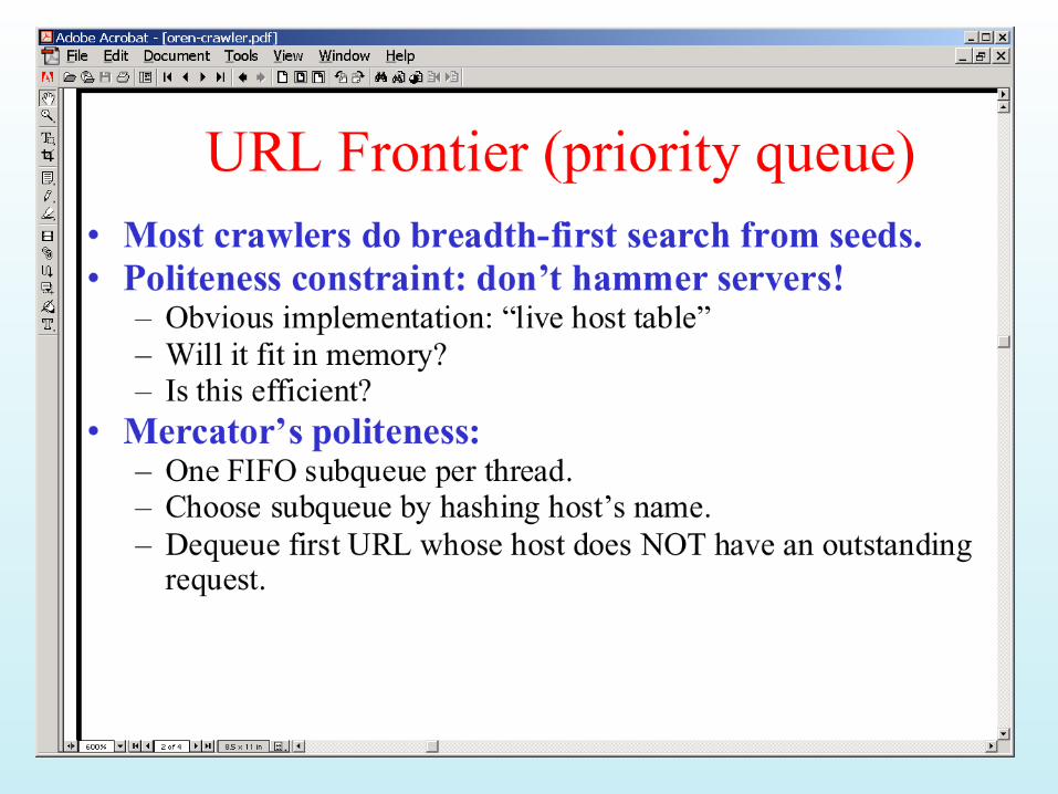
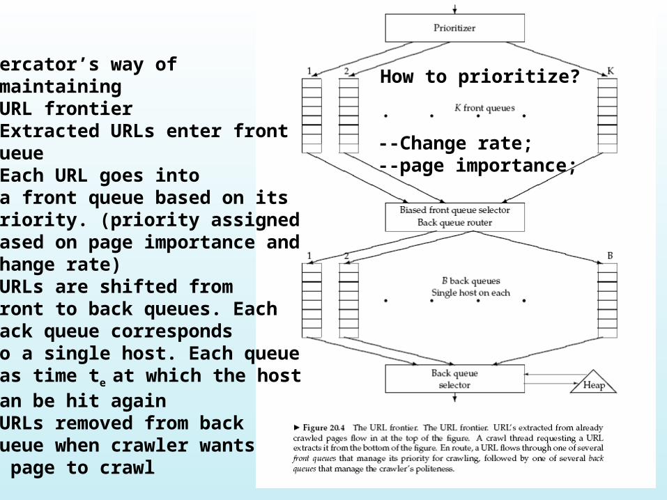
Mercator’s way of maintaining URL frontierExtracted URLs enter frontqueueEach URL goes into a front queue based on itsPriority. (priority assignedBased on page importance andChange rate)URLs are shifted fromFront to back queues. EachBack queue correspondsTo a single host. Each queueHas time te
at which the host Can be hit againURLs removed from backQueue when crawler wantsA page to crawl
How to prioritize?
--Change rate;--page importance;
Robot (4)
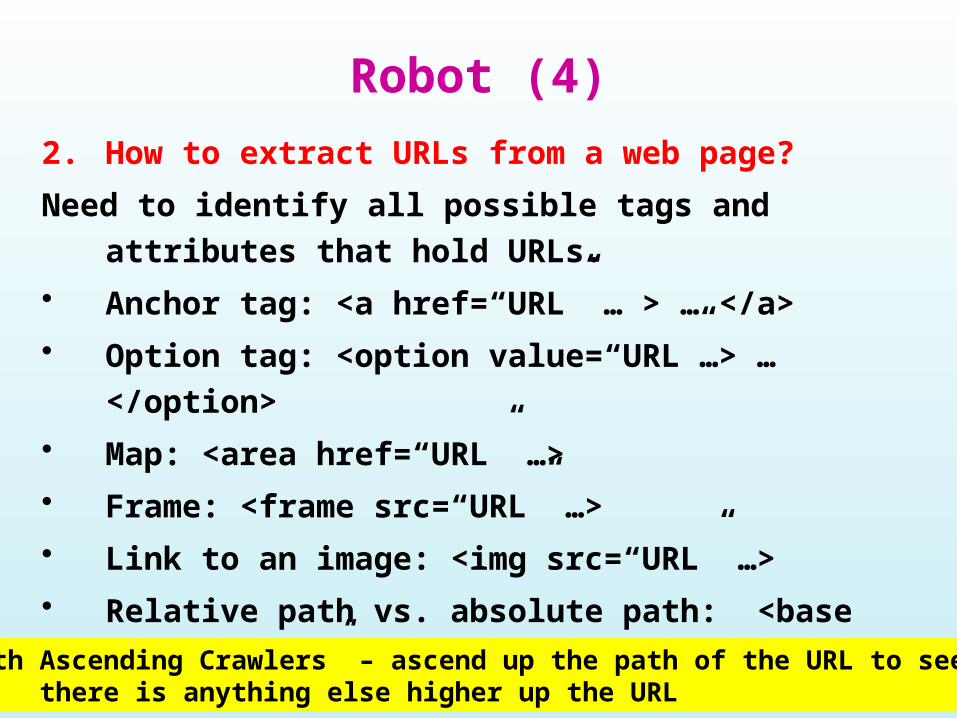
2. How to extract URLs from a web page?
Need to identify all possible tags and attributes that hold
URLs.
• Anchor tag: <a href=“URL” … > … </a>
• Option tag: <option value=“URL”…> … </option>
• Map: <area href=“URL” …>
• Frame: <frame src=“URL” …>
• Link to an image: <img src=“URL” …>
• Relative path vs. absolute path: <base href= …>
“Path Ascending Crawlers” – ascend up the path of the URL to see if there is anything else higher up the URL
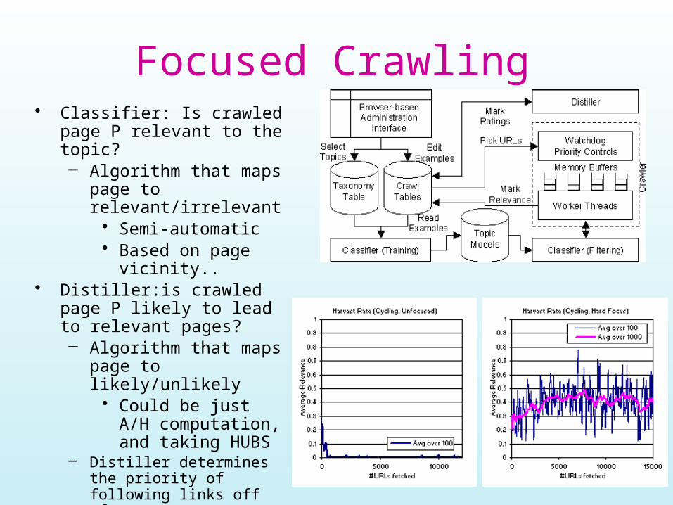
Focused Crawling• Classifier: Is crawled page P
relevant to the topic?– Algorithm that maps page
to relevant/irrelevant• Semi-automatic• Based on page
vicinity..• Distiller:is crawled page P
likely to lead to relevant pages?– Algorithm that maps page
to likely/unlikely• Could be just A/H
computation, and taking HUBS
– Distiller determines the priority of following links off of P

Connectivity Server..
• All the link-analysis techniques need information on who is pointing to who– In particular, need the back-link information
• Connectivity server provides this. It can be seen as an inverted index– Forward: Page id id’s of forward links– Inverted: Page id id’s of pages linking to it

What is the best way to exploit all these machines?
• What kind of parallelism?– Can’t be fine-grained– Can’t depend on shared-memory (which
could fail)– Worker machines should be largely
allowed to do their work independently– We may not even know how many (and
which) machines may be available…

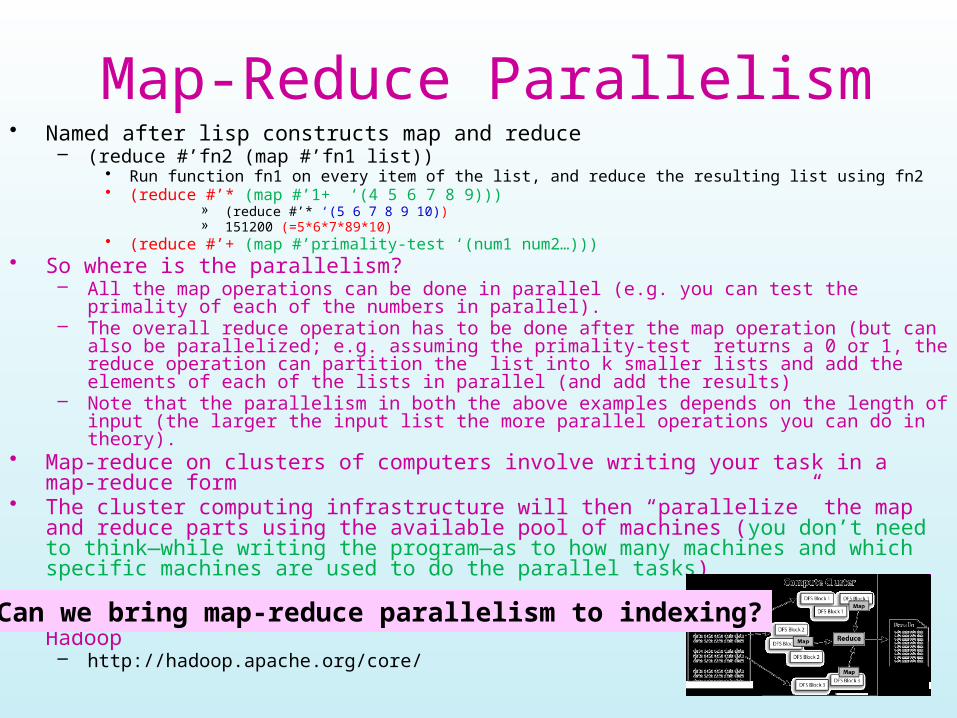
Map-Reduce Parallelism• Named after lisp constructs map and reduce
– (reduce #’fn2 (map #’fn1 list))• Run function fn1 on every item of the list, and reduce the resulting list using fn2• (reduce #’* (map #’1+ ‘(4 5 6 7 8 9)))
» (reduce #’* ‘(5 6 7 8 9 10))» 151200 (=5*6*7*89*10)
• (reduce #’+ (map #’primality-test ‘(num1 num2…)))• So where is the parallelism?
– All the map operations can be done in parallel (e.g. you can test the primality of each of the numbers in parallel).
– The overall reduce operation has to be done after the map operation (but can also be parallelized; e.g. assuming the primality-test returns a 0 or 1, the reduce operation can partition the list into k smaller lists and add the elements of each of the lists in parallel (and add the results)
– Note that the parallelism in both the above examples depends on the length of input (the larger the input list the more parallel operations you can do in theory).
• Map-reduce on clusters of computers involve writing your task in a map-reduce form• The cluster computing infrastructure will then “parallelize” the map and reduce parts using the
available pool of machines (you don’t need to think—while writing the program—as to how many machines and which specific machines are used to do the parallel tasks)
• An open source environment that provides such an infrastructure is Hadoop – http://hadoop.apache.org/core/
Qn: Can we bring map-reduce parallelism to indexing?
MapReduce
These slides are from Rajaram & Ullman
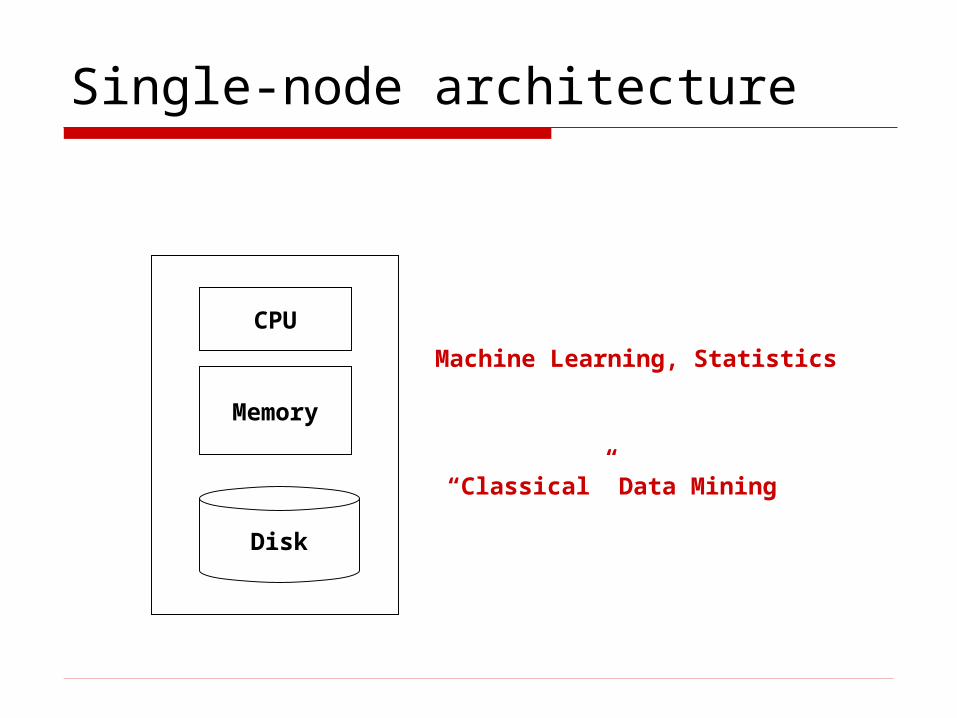
Single-node architecture
Memory
Disk
CPU
Machine Learning, Statistics
“Classical” Data Mining
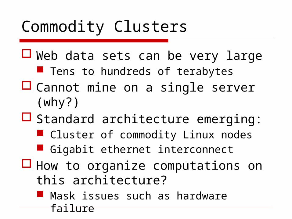
Commodity Clusters
Web data sets can be very large Tens to hundreds of terabytes
Cannot mine on a single server (why?) Standard architecture emerging:
Cluster of commodity Linux nodes Gigabit ethernet interconnect
How to organize computations on this architecture? Mask issues such as hardware failure
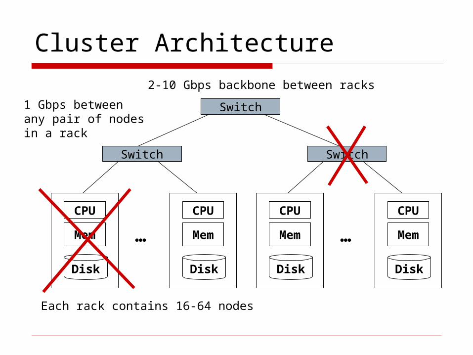
Cluster Architecture
Mem
Disk
CPU
Mem
Disk
CPU
…
Switch
Each rack contains 16-64 nodes
Mem
Disk
CPU
Mem
Disk
CPU
…
Switch
Switch1 Gbps between any pair of nodesin a rack
2-10 Gbps backbone between racks
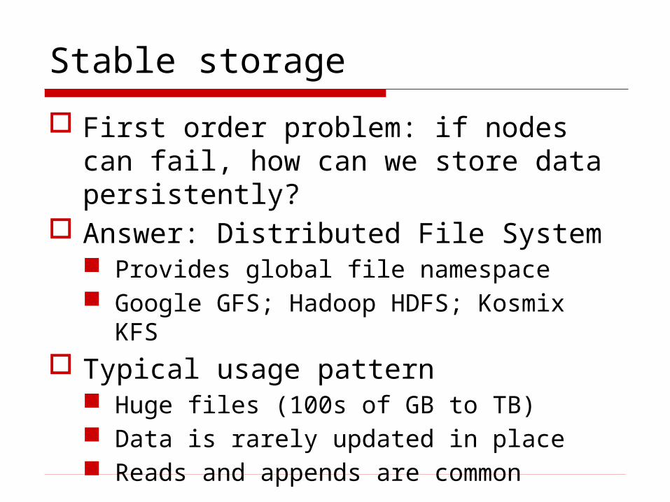
Stable storage
First order problem: if nodes can fail, how can we store data persistently?
Answer: Distributed File System Provides global file namespace Google GFS; Hadoop HDFS; Kosmix KFS
Typical usage pattern Huge files (100s of GB to TB) Data is rarely updated in place Reads and appends are common
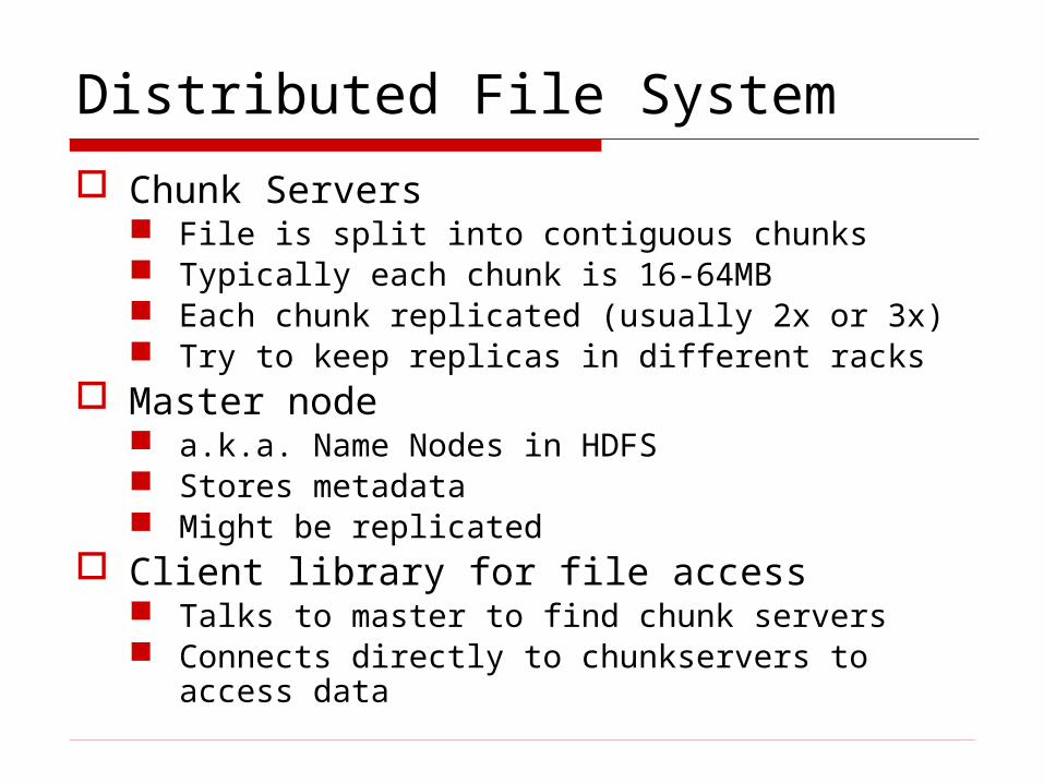
Distributed File System
Chunk Servers File is split into contiguous chunks Typically each chunk is 16-64MB Each chunk replicated (usually 2x or 3x) Try to keep replicas in different racks
Master node a.k.a. Name Nodes in HDFS Stores metadata Might be replicated
Client library for file access Talks to master to find chunk servers Connects directly to chunkservers to access data
Warm up: Word Count
We have a large file of words, one word to a line
Count the number of times each distinct word appears in the file
Sample application: analyze web server logs to find popular URLs
Word Count (2)
Case 1: Entire file fits in memory Case 2: File too large for mem, but all
<word, count> pairs fit in mem Case 3: File on disk, too many distinct
words to fit in memory sort datafile | uniq –c
Word Count (3)
To make it slightly harder, suppose we have a large corpus of documents
Count the number of times each distinct word occurs in the corpus words(docs/*) | sort | uniq -c where words takes a file and outputs the
words in it, one to a line The above captures the essence of
MapReduce Great thing is it is naturally parallelizable
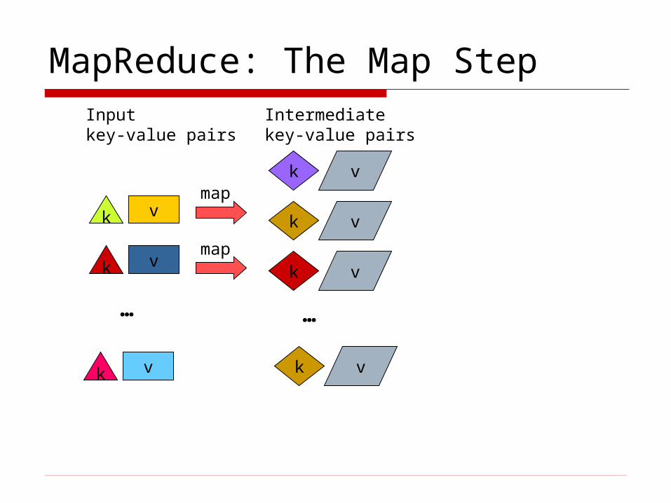
MapReduce: The Map Step
vk
k v
k v
mapvk
vk
…
k vmap
Inputkey-value pairs
Intermediatekey-value pairs
…
k v
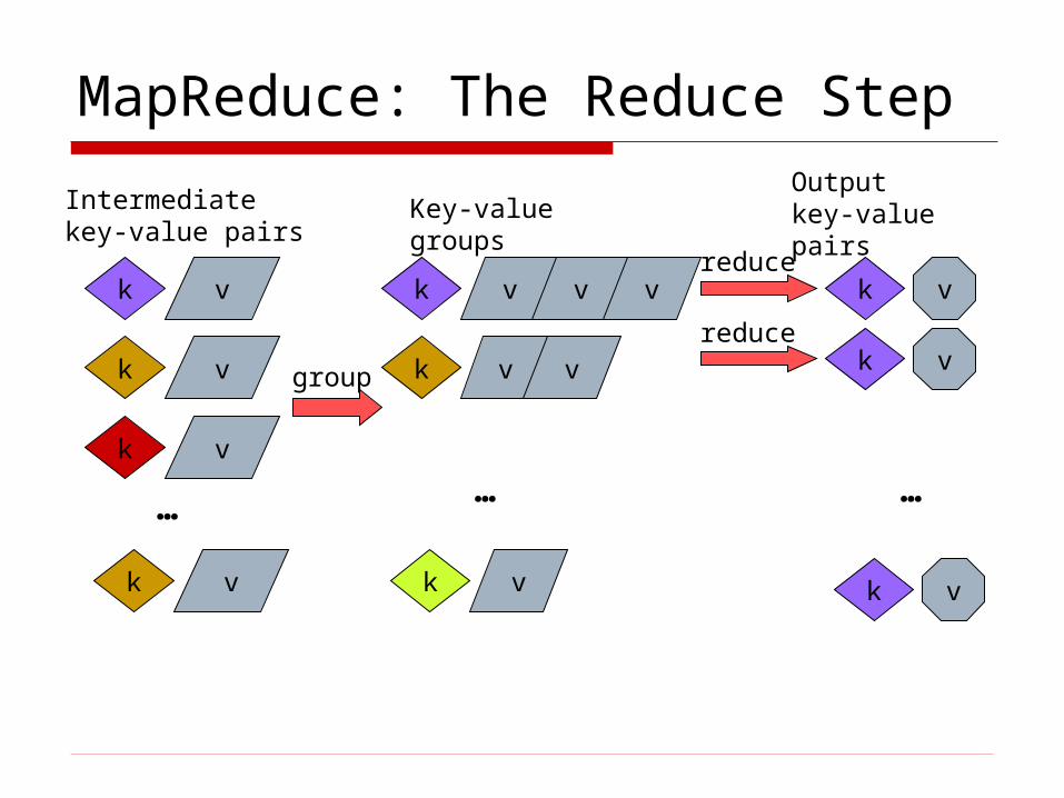
MapReduce: The Reduce Step
k v
…
k v
k v
k v
Intermediatekey-value pairs
group
reduce
reduce
k v
k v
k v
…
k v
…
k v
k v v
v v
Key-value groupsOutput key-value pairs
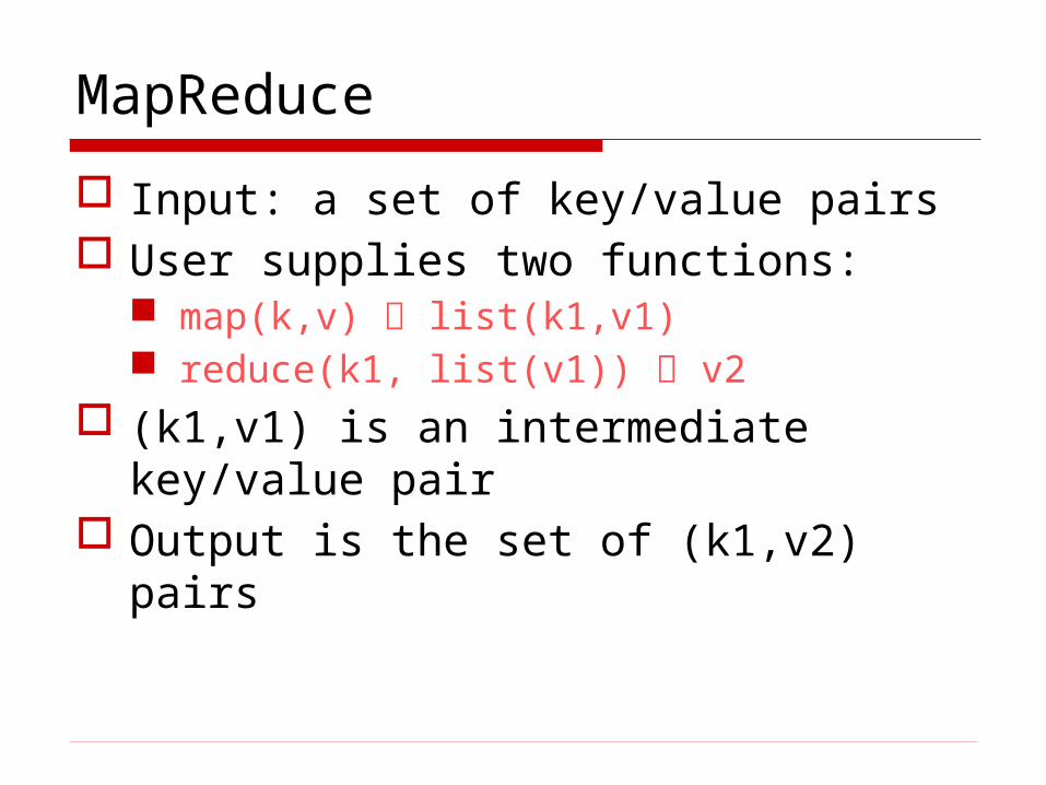
MapReduce
Input: a set of key/value pairs User supplies two functions:
map(k,v) list(k1,v1) reduce(k1, list(v1)) v2
(k1,v1) is an intermediate key/value pair
Output is the set of (k1,v2) pairs
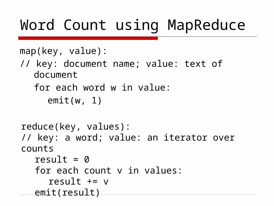
Word Count using MapReduce
map(key, value):// key: document name; value: text of document
for each word w in value:emit(w, 1)
reduce(key, values):// key: a word; value: an iterator over counts
result = 0for each count v in values:
result += vemit(result)
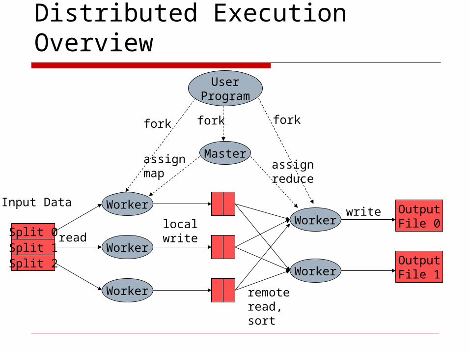
Distributed Execution Overview User
Program
Worker
Worker
Master
Worker
Worker
Worker
fork fork fork
assignmap
assignreduce
readlocalwrite
remoteread,sort
OutputFile 0
OutputFile 1
write
Split 0Split 1Split 2
Input Data
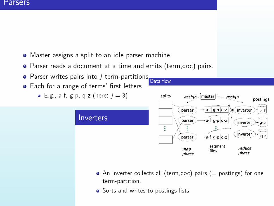
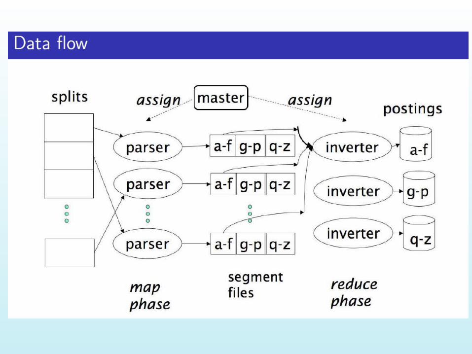
Data flow
Input, final output are stored on a distributed file system Scheduler tries to schedule map tasks
“close” to physical storage location of input data
Intermediate results are stored on local FS of map and reduce workers
Output is often input to another map reduce task
Coordination
Master data structures Task status: (idle, in-progress, completed) Idle tasks get scheduled as workers
become available When a map task completes, it sends the
master the location and sizes of its R intermediate files, one for each reducer
Master pushes this info to reducers Master pings workers periodically to
detect failures
Failures
Map worker failure Map tasks completed or in-progress at
worker are reset to idle Reduce workers are notified when task is
rescheduled on another worker Reduce worker failure
Only in-progress tasks are reset to idle Master failure
MapReduce task is aborted and client is notified
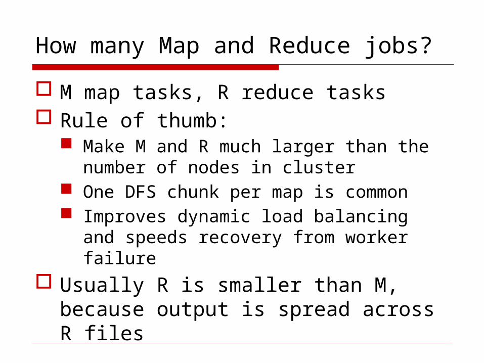
How many Map and Reduce jobs?
M map tasks, R reduce tasks Rule of thumb:
Make M and R much larger than the number of nodes in cluster
One DFS chunk per map is common Improves dynamic load balancing and
speeds recovery from worker failure Usually R is smaller than M, because
output is spread across R files
Reading
Jeffrey Dean and Sanjay Ghemawat,
MapReduce: Simplified Data Processing on Large Clusters
http://labs.google.com/papers/mapreduce.html
Sanjay Ghemawat, Howard Gobioff, and Shun-Tak Leung, The Google File System
http://labs.google.com/papers/gfs.html
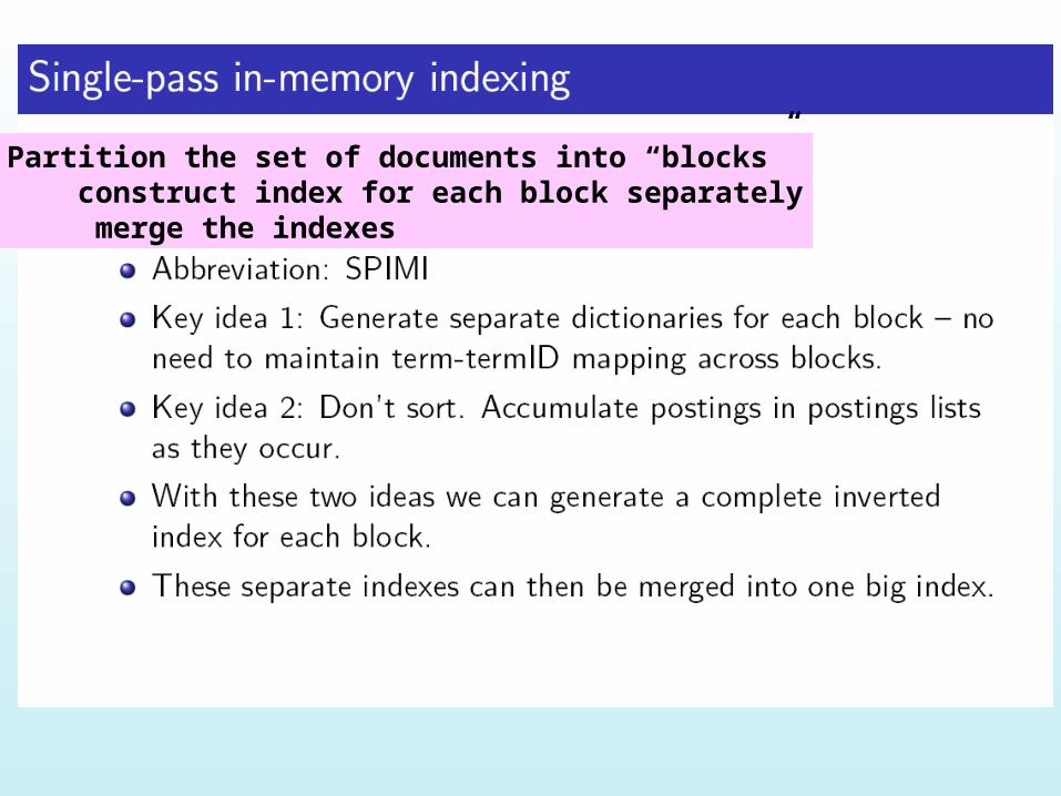
Partition the set of documents into “blocks” construct index for each block separately merge the indexes
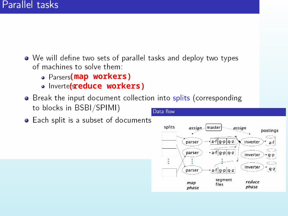
(map workers)(reduce workers)
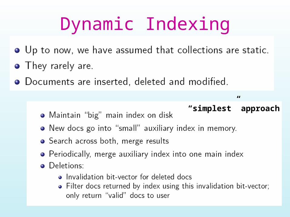
Dynamic Indexing
“simplest” approach

Efficient Computation of Pagerank
How to power-iterate on the web-scale matrix?
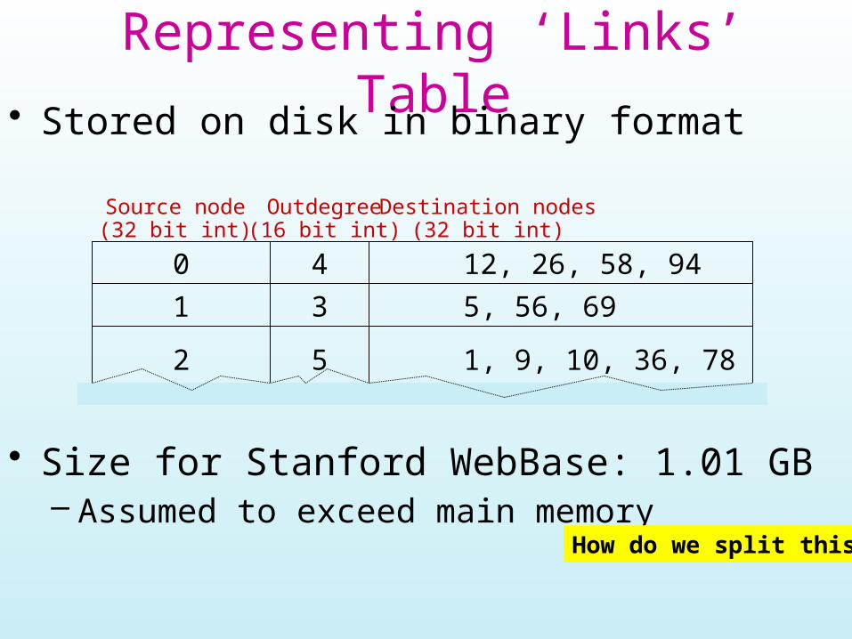
Representing ‘Links’ Table• Stored on disk in binary format
• Size for Stanford WebBase: 1.01 GB– Assumed to exceed main memory
0
1
2
4
3
5
12, 26, 58, 94
5, 56, 69
1, 9, 10, 36, 78
Source node(32 bit int)
Outdegree(16 bit int)
Destination nodes(32 bit int)
How do we split this?
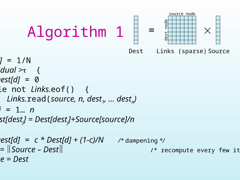
Algorithm 1 =
Dest Links (sparse) Source
source node
dest
nod
e
s Source[s] = 1/Nwhile residual > { d Dest[d] = 0 while not Links.eof() { Links.read(source, n, dest1, … destn) for j = 1… n Dest[destj] = Dest[destj]+Source[source]/n } d Dest[d] = c * Dest[d] + (1-c)/N /* dampening */
residual = Source – Dest /* recompute every few iterations */
Source = Dest}
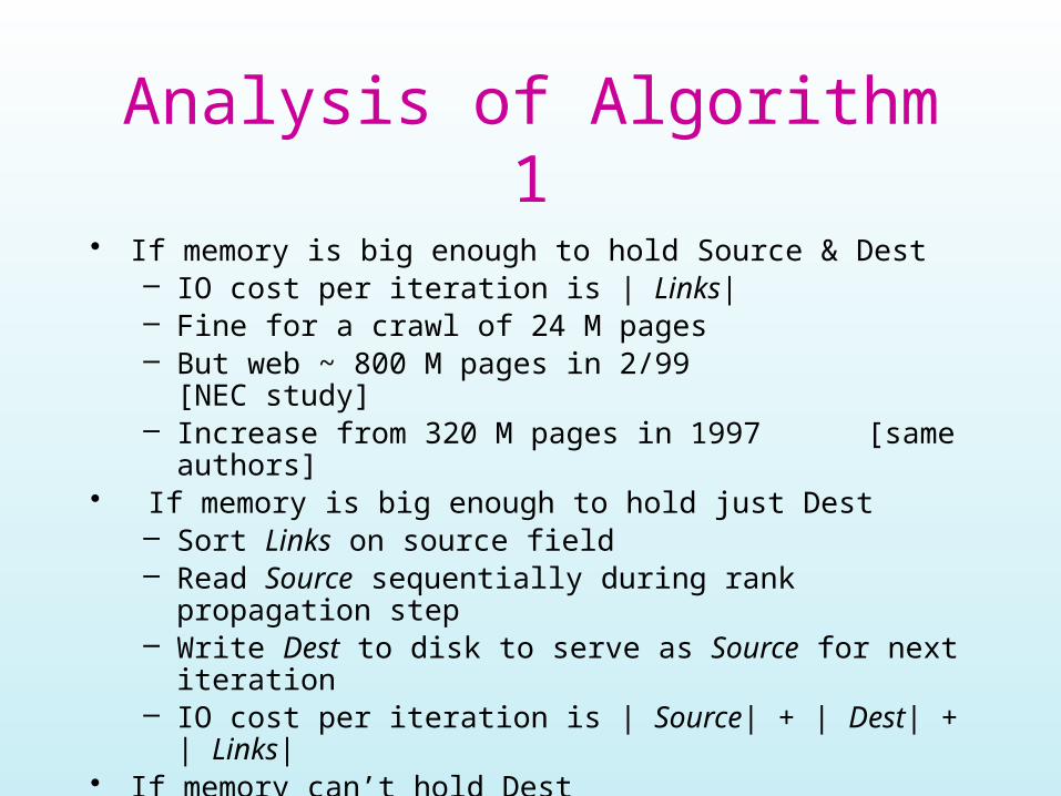
Analysis of Algorithm 1
• If memory is big enough to hold Source & Dest– IO cost per iteration is | Links|– Fine for a crawl of 24 M pages– But web ~ 800 M pages in 2/99 [NEC study]– Increase from 320 M pages in 1997 [same authors]
• If memory is big enough to hold just Dest– Sort Links on source field– Read Source sequentially during rank propagation step– Write Dest to disk to serve as Source for next iteration– IO cost per iteration is | Source| + | Dest| + | Links|
• If memory can’t hold Dest– Random access pattern will make working set = | Dest| – Thrash!!!
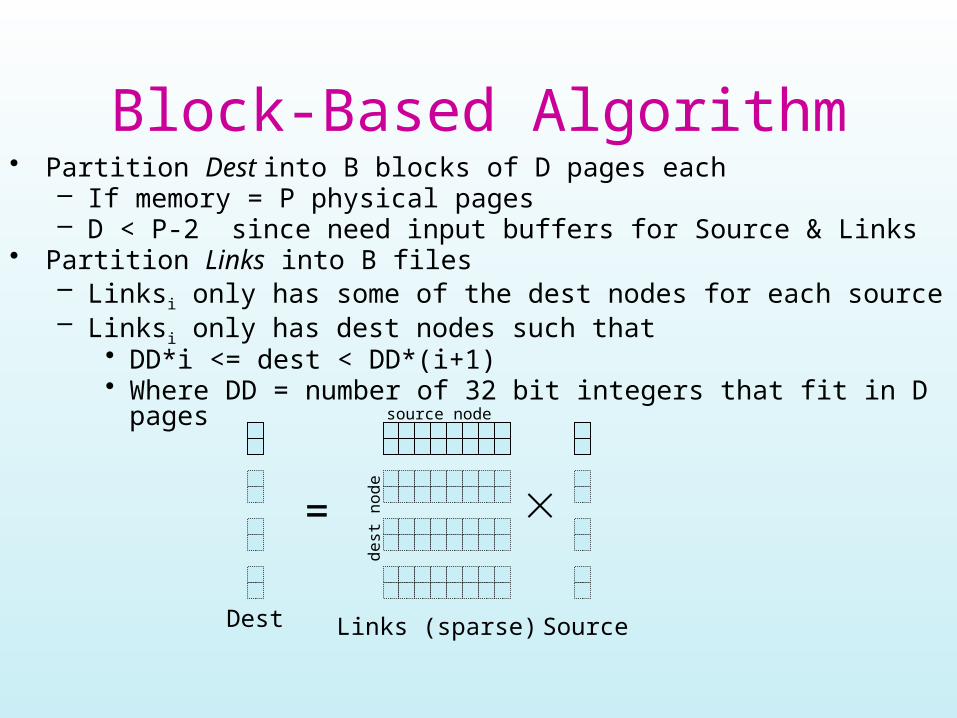
Block-Based Algorithm• Partition Dest into B blocks of D pages each
– If memory = P physical pages– D < P-2 since need input buffers for Source & Links
• Partition Links into B files– Linksi only has some of the dest nodes for each source– Linksi only has dest nodes such that
• DD*i <= dest < DD*(i+1)• Where DD = number of 32 bit integers that fit in D pages
=
Dest Links (sparse) Source
source node
dest
nod
e
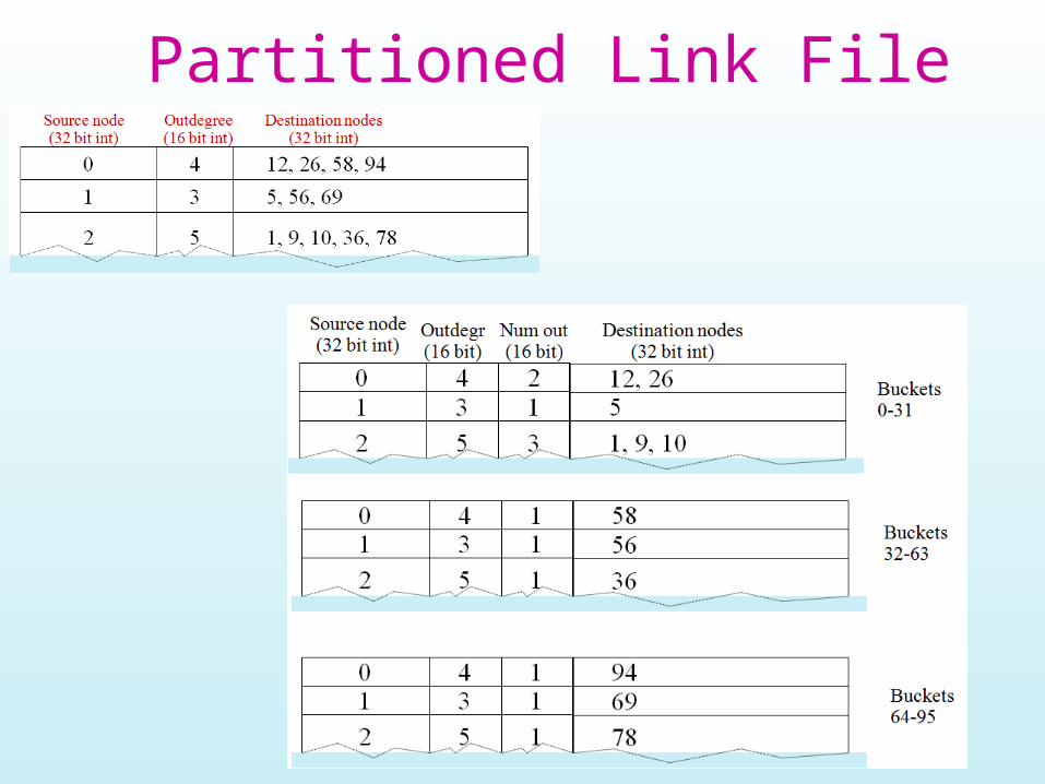
Partitioned Link File
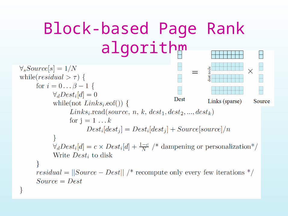
Block-based Page Rank algorithm
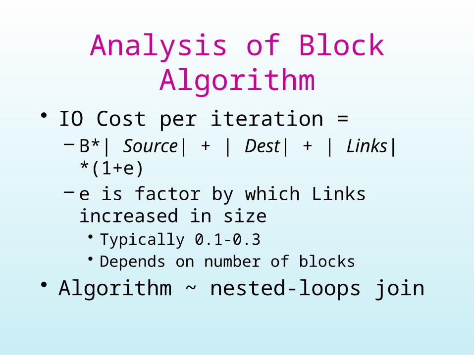
Analysis of Block Algorithm
• IO Cost per iteration = – B*| Source| + | Dest| + | Links|*(1+e)– e is factor by which Links increased in size
• Typically 0.1-0.3• Depends on number of blocks
• Algorithm ~ nested-loops join
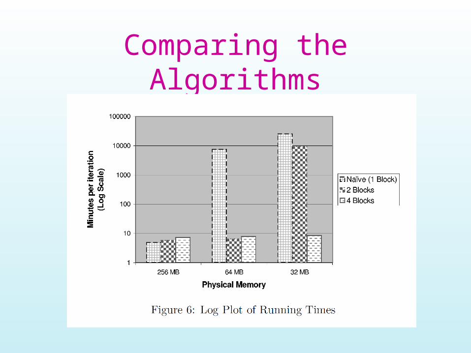
Comparing the Algorithms
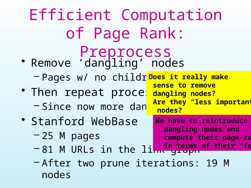
Efficient Computation of Page Rank: Preprocess
• Remove ‘dangling’ nodes– Pages w/ no children
• Then repeat process– Since now more danglers
• Stanford WebBase– 25 M pages– 81 M URLs in the link graph– After two prune iterations: 19 M nodes
Does it really make sense to remove dangling nodes? Are they “less important” nodes?
We have to reintroduce dangling nodes and compute their page ranks in terms of their “fans”
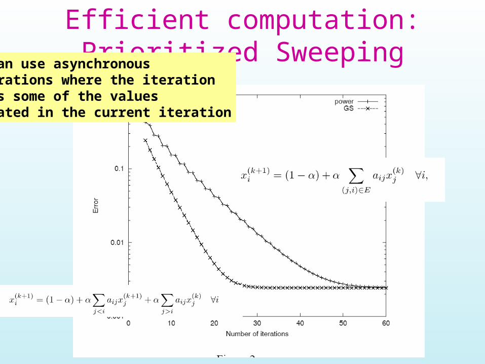
Efficient computation: Prioritized SweepingWe can use asynchronous
iterations where the iteration uses some of the values updated in the current iteration

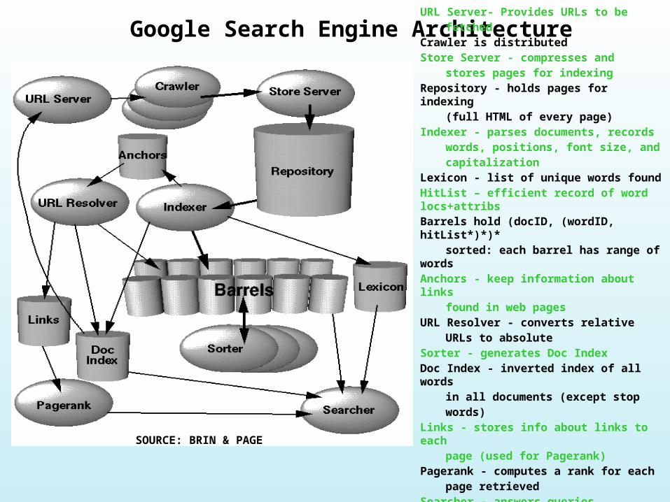
Google Search Engine Architecture
SOURCE: BRIN & PAGE
URL Server- Provides URLs to befetched
Crawler is distributedStore Server - compresses and
stores pages for indexingRepository - holds pages for indexing
(full HTML of every page)Indexer - parses documents, records
words, positions, font size, andcapitalization
Lexicon - list of unique words foundHitList – efficient record of word locs+attribsBarrels hold (docID, (wordID, hitList*)*)*
sorted: each barrel has range of wordsAnchors - keep information about links
found in web pagesURL Resolver - converts relative
URLs to absoluteSorter - generates Doc IndexDoc Index - inverted index of all words
in all documents (except stopwords)
Links - stores info about links to eachpage (used for Pagerank)
Pagerank - computes a rank for eachpage retrieved
Searcher - answers queries
Major Data Structures
• Big Files– virtual files spanning multiple file systems– addressable by 64 bit integers– handles allocation & deallocation of File
Descriptions since the OS’s is not enough– supports rudimentary compression
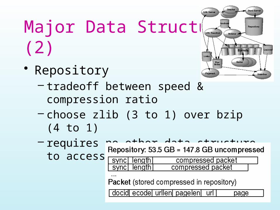
Major Data Structures (2)
• Repository– tradeoff between speed & compression
ratio– choose zlib (3 to 1) over bzip (4 to 1)– requires no other data structure to access
it
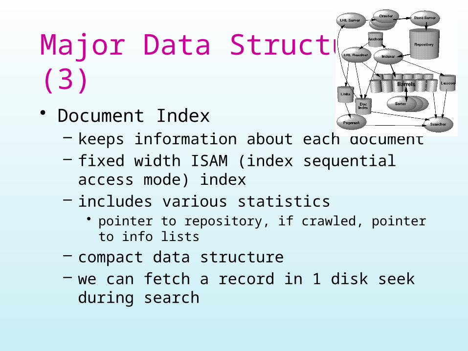
Major Data Structures (3)
• Document Index– keeps information about each document– fixed width ISAM (index sequential access mode)
index– includes various statistics
• pointer to repository, if crawled, pointer to info lists
– compact data structure– we can fetch a record in 1 disk seek during search
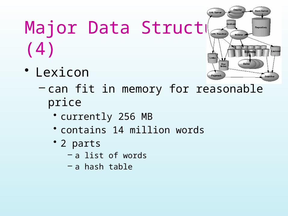
Major Data Structures (4)
• Lexicon– can fit in memory for reasonable price
• currently 256 MB• contains 14 million words• 2 parts
– a list of words– a hash table
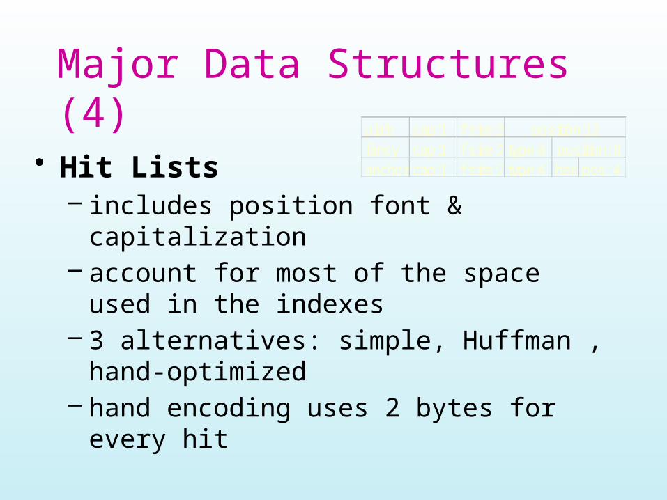
Major Data Structures (4)
• Hit Lists– includes position font & capitalization– account for most of the space used in the
indexes– 3 alternatives: simple, Huffman , hand-
optimized– hand encoding uses 2 bytes for every hit
f size:3cap:1plaintype:4f size:7cap:1fancy
pos: 4hash:4type:4f size:7cap:1anchor
position:12position: 8
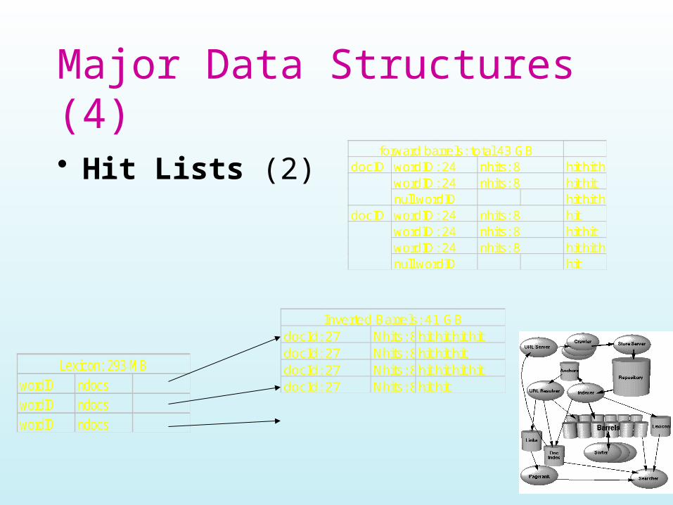
Major Data Structures (4)
• Hit Lists (2) hit hit hitdocIDhit hithit hit hithitdocIDhit hithit hit hithit
nhits: 8wordID: 24
wordID: 24 nhits: 8
nhits: 8
nhits: 8wordID: 24null wordID
forward barrels: total 43 GB
null wordID
nhits: 8wordID: 24
wordID: 24
ndocswordIDndocswordIDndocswordID
Lexicon: 293 MB
Nhits: 8Nhits: 8Nhits: 8Nhits: 8hit hit
Inverted Barrels: 41 GBhit hit hit hithit hit hithit hit hit hit
docId: 27docId: 27docId: 27docId: 27
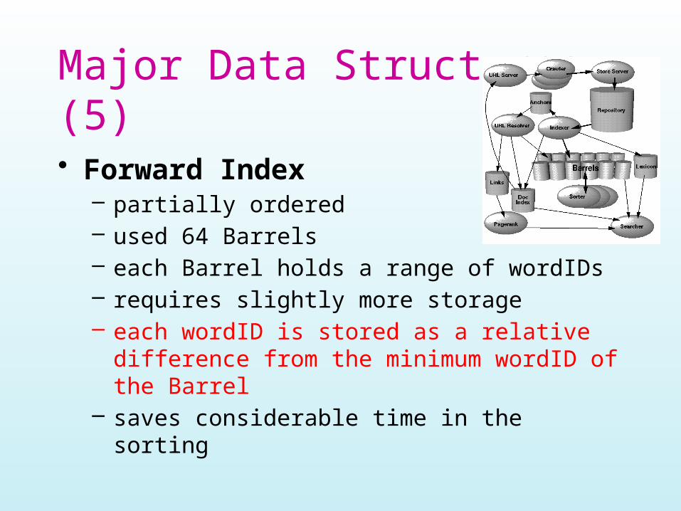
Major Data Structures (5)
• Forward Index– partially ordered– used 64 Barrels– each Barrel holds a range of wordIDs– requires slightly more storage– each wordID is stored as a relative difference from
the minimum wordID of the Barrel– saves considerable time in the sorting
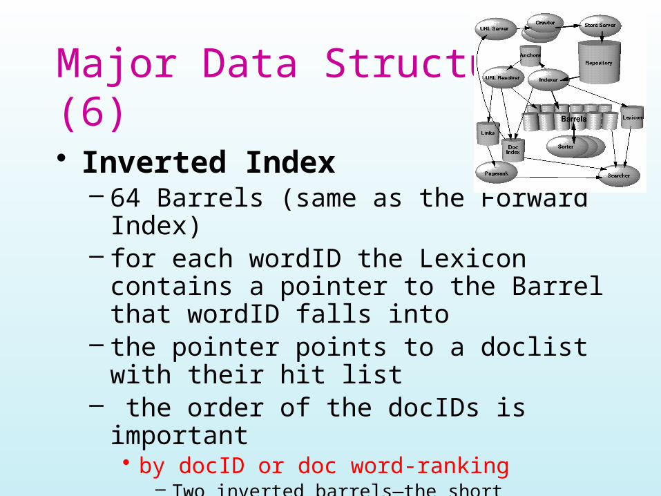
Major Data Structures (6)
• Inverted Index– 64 Barrels (same as the Forward Index)– for each wordID the Lexicon contains a
pointer to the Barrel that wordID falls into– the pointer points to a doclist with their hit
list– the order of the docIDs is important
• by docID or doc word-ranking– Two inverted barrels—the short barrel/full barrel
Major Data Structures (7)
• Crawling the Web– fast distributed crawling system– URLserver & Crawlers are implemented in phyton– each Crawler keeps about 300 connection open– at peek time the rate - 100 pages, 600K per second– uses: internal cached DNS lookup
– synchronized IO to handle events– number of queues
– Robust & Carefully tested
Major Data Structures (8)
• Indexing the Web– Parsing
• should know to handle errors– HTML typos– kb of zeros in a middle of a TAG– non-ASCII characters– HTML Tags nested hundreds deep
• Developed their own Parser– involved a fair amount of work– did not cause a bottleneck
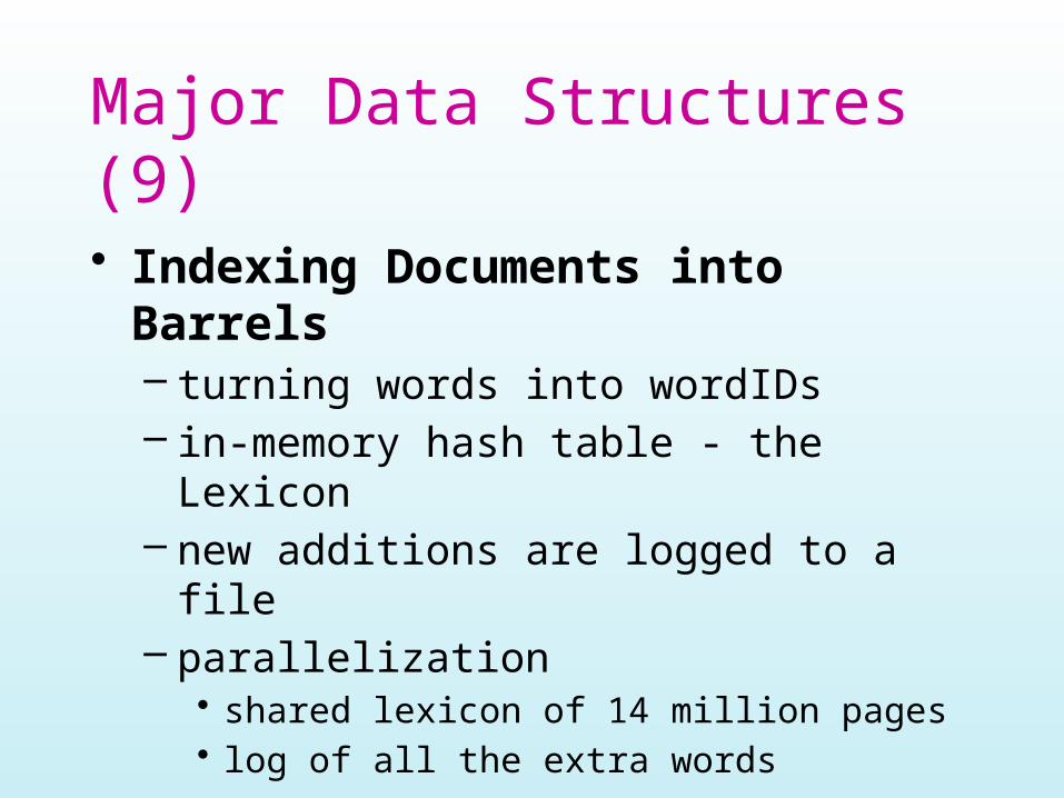
Major Data Structures (9)
• Indexing Documents into Barrels– turning words into wordIDs– in-memory hash table - the Lexicon– new additions are logged to a file– parallelization
• shared lexicon of 14 million pages• log of all the extra words
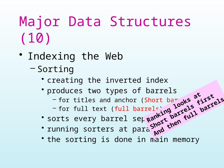
Major Data Structures (10)
• Indexing the Web– Sorting
• creating the inverted index• produces two types of barrels
– for titles and anchor (Short barrels)– for full text (full barrels)
• sorts every barrel separately• running sorters at parallel• the sorting is done in main memory
Ranking looks at
Short barrels first
And then full barrels
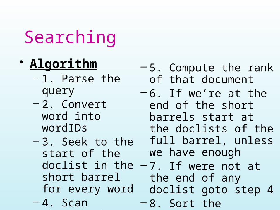
Searching• Algorithm
– 1. Parse the query– 2. Convert word
into wordIDs– 3. Seek to the start
of the doclist in the short barrel for every word
– 4. Scan through the doclists until there is a document that matches all of the search terms
– 5. Compute the rank of that document
– 6. If we’re at the end of the short barrels start at the doclists of the full barrel, unless we have enough
– 7. If were not at the end of any doclist goto step 4
– 8. Sort the documents by rank return the top K• (May jump here after 40k
pages)
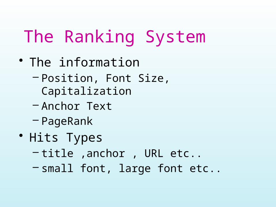
The Ranking System• The information
– Position, Font Size, Capitalization– Anchor Text– PageRank
• Hits Types– title ,anchor , URL etc..– small font, large font etc..
The Ranking System (2)
• Each Hit type has it’s own weight– Counts weights increase linearly with counts at first
but quickly taper off this is the IR score of the doc– (IDF weighting??)
• the IR is combined with PageRank to give the final Rank
• For multi-word query– A proximity score for every set of hits with a
proximity type weight• 10 grades of proximity
Feedback
• A trusted user may optionally evaluate the results
• The feedback is saved• When modifying the ranking function we
can see the impact of this change on all previous searches that were ranked
Results
• Produce better results than major commercial search engines for most searches
• Example: query “bill clinton”– return results from the “Whitehouse.gov”– email addresses of the president– all the results are high quality pages– no broken links– no bill without clinton & no clinton without bill
Storage Requirements
• Using Compression on the repository• about 55 GB for all the data used by the
SE• most of the queries can be answered by
just the short inverted index• with better compression, a high quality
SE can fit onto a 7GB drive of a new PC
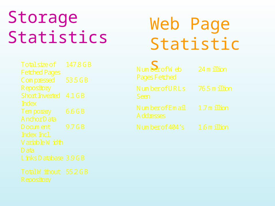
Storage Statistics
Total size ofFetched Pages
147.8 GB
CompressedRepository
53.5 GB
Short InvertedIndex
4.1 GB
TemporaryAnchor Data
6.6 GB
DocumentIndex Incl.Variable WidthData
9.7 GB
Links Database 3.9 GB
Total WithoutRepository
55.2 GB
Web Page Statistics
Number of WebPages Fetched
24 million
Number of URLsSeen
76.5 million
Number of EmailAddresses
1.7 million
Number of 404’s 1.6 million
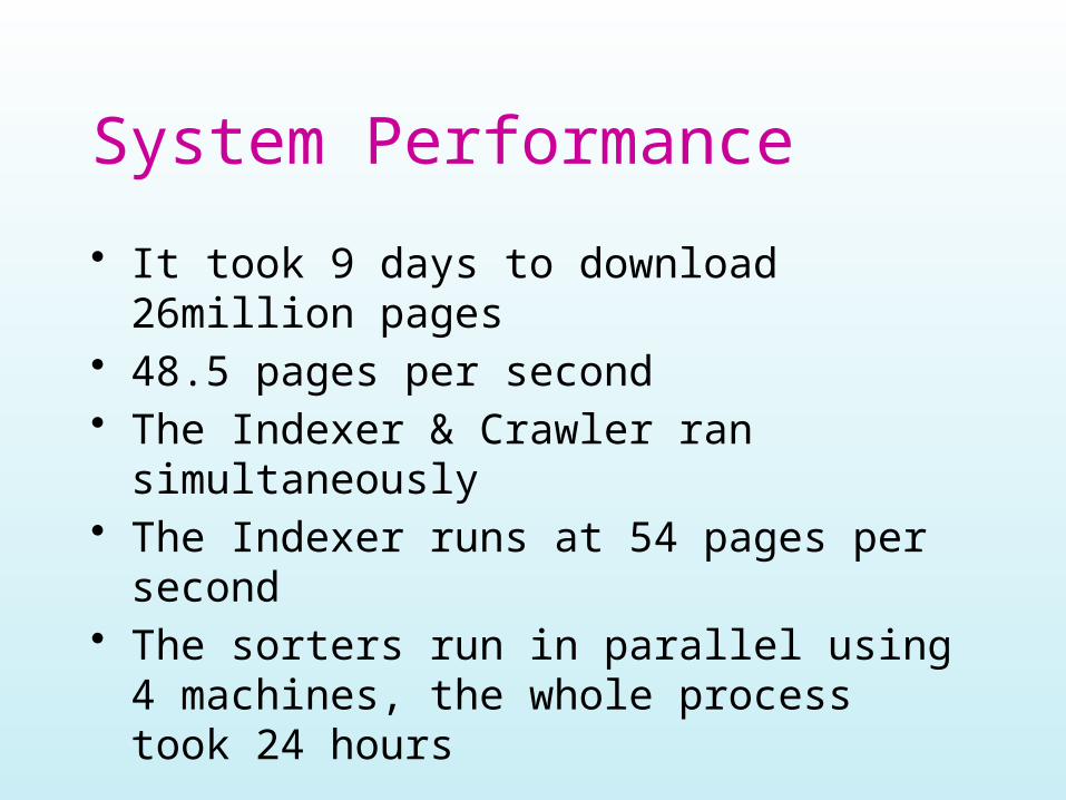
System Performance
• It took 9 days to download 26million pages• 48.5 pages per second• The Indexer & Crawler ran simultaneously• The Indexer runs at 54 pages per second• The sorters run in parallel using 4 machines,
the whole process took 24 hours