Embed Size (px)
Citation preview
THE BOND MARKET’S q∗
THOMAS PHILIPPON
I propose an implementation of the q-theory of investment using bond pricesinstead of equity prices. Credit risk makes corporate bond prices sensitive to futureasset values, and q can be inferred from bond prices. With aggregate U.S. data,the bond market’s q fits the investment equation six times better than the usualmeasure of q, it drives out cash flows, and it reduces the implied adjustment costsby more than an order of magnitude. Theoretical interpretations for these resultsare discussed.
I. INTRODUCTION
In his 1969 article, James Tobin argued that “the rate ofinvestment—the speed at which investors wish to increase thecapital stock—should be related, if to anything, to q, the valueof capital relative to its replacement cost” (Tobin 1969, p. 21).Tobin also recognized, however, that q must depend on “expecta-tions, estimates of risk, attitudes towards risk, and a host of otherfactors,” and he concluded that “it is not to be expected that theessential impact of [. . . ] financial events will be easy to measurein the absence of direct observation of the relevant variables (q inthe models).” The quest for an observable proxy for q was thereforerecognized as a crucial objective from the very beginning.
Subsequent research succeeded in integrating Tobin’s ap-proach with the neoclassical investment theory of Jorgenson(1963). Lucas and Prescott (1971) proposed a dynamic model ofinvestment with convex adjustment costs, and Abel (1979) showedthat the rate of investment is optimal when the marginal cost ofinstallment is equal to q − 1. Finally, Hayashi (1982) showed that,under perfect competition and constant returns to scale, marginalq (the market value of an additional unit of capital divided byits replacement cost) is equal to average q (the market valueof existing capital divided by its replacement cost). Because av-erage q is observable, the theory became empirically relevant.
∗This paper was first circulated under the title “The y-Theory of Investment.”I thank Robert Barro (the editor), three anonymous referees, Daron Acemoglu,Mark Aguiar, Manuel Amador, Luca Benzoni, Olivier Blanchard, Xavier Gabaix,Mark Gertler, Simon Gilchrist, Bob Hall, Guido Lorenzoni, Sydney Ludvigson,Pete Kyle, Lasse Pedersen, Christina Romer, David Romer, Ivan Werning, ToniWhited, Jeff Wurgler, Egon Zakrajsek, and seminar participants at NYU, MIT, theSED 2007, London Business School, Ente Einaudi (Rome), University of Salerno,Toulouse University, Duke University, and the NBER Summer Institutes 2006 and2007. Peter Gross provided excellent research assistance.
C© 2009 by the President and Fellows of Harvard College and the Massachusetts Institute ofTechnology.The Quarterly Journal of Economics, August 2009
1011
at New
York U
niversity School of Law
on September 11, 2013
http://qje.oxfordjournals.org/D
ownloaded from
1012 QUARTERLY JOURNAL OF ECONOMICS
Unfortunately, its implementation proved disappointing. The in-vestment equation fits poorly, leaves large unexplained residualscorrelated with cash flows, and implies implausible parameters forthe adjustment cost function (see Summers [1981] for an early con-tribution, and Hassett and Hubbard [1997] and Caballero [1999]for recent literature reviews).
Several theories have been proposed to explain this failure.Firms could have market power, and might not operate underconstant returns to scale. Adjustment costs might not be convex(Dixit and Pindyck 1994; Caballero and Engle 1999). Firms mightbe credit-constrained (Fazzari, Hubbard, and Petersen 1988;Bernanke and Gertler 1989). Finally, there could be measurementerrors and aggregation biases in the capital stock or the rate ofinvestment. None of these explanations is fully satisfactory, how-ever. The evidence for constant returns and price-taking seemsquite strong (Hall 2003). Adjustment costs are certainly not con-vex at the plant level, but it is not clear that it really matters in theaggregate (Thomas 2002; Hall 2004), although this is still a con-troversial issue (Bachmann, Caballero, and Engel 2006). Gomes(2001) shows that Tobin’s q should capture most of investmentdynamics even when there are credit constraints. Heterogeneityand aggregation do not seem to create strong biases (Hall 2004).
In fact, an intriguing message comes out of the more recentempirical research: the market value of equity seems to be the cul-prit for the empirical failure of the investment equation. Gilchristand Himmelberg (1995), following Abel and Blanchard (1986),use VARs to forecast cash flows and to construct q, and they findthat it performs better than the traditional measure based onequity prices. Cumins, Hasset, and Oliner (2006) use analysts’forecasts instead of VAR forecasts and reach similar conclusions.Erickson and Whited (2000, 2006) use GMM estimators to purgeq from measurement errors. They find that only 40% of observedvariations are due to fundamental changes, and, once again, thatmarket values contain large “measurement errors.”
Applied research has therefore reached an uncomfortable sit-uation, where the benchmark investment equation appears to besuccessful only when market prices are not used to construct q.This is unfortunate, because Tobin’s insight was precisely to linkobserved quantities and market prices. The contribution of thispaper is to show that a market-based measure of q can be con-structed from corporate bond prices and that this measure per-forms much better than the traditional one.
at New
York U
niversity School of Law
on September 11, 2013
http://qje.oxfordjournals.org/D
ownloaded from
THE BOND MARKET’S q 1013
Why would the bond market’s q perform better than the usualmeasure? There are several possible explanations, two of whichare discussed in details in this paper. The first explanation isthat total firm value includes the value of growth options, thatis, opportunities to expand into new areas and new technologies.With enough skewness, these growth options end up affectingequity prices much more than bond prices. If, in addition, thesegrowth options are unrelated to existing operations, they do notaffect current capital expenditures. As a result, bond prices aremore closely related to the existing technology’s q, while equityprices reflect organizational rents.
A second possible explanation is that the bond market is lesssusceptible to bubbles than the equity market. In fact, there isempirical and theoretical support for the idea that mispricing ismore likely to happen when returns are positively skewed. Bar-beris and Huang (2007) show that cumulative prospect theorycan explain how a positively skewed security becomes overpriced.Brunnermeier, Gollier, and Parker (2007) argue that preferencefor skewness arises endogenously because investors choose tobe optimistic about the states associated with the most skewedArrow–Debreu securities. Empirically, Mitton and Vorkink (2007)document that underdiversification is largely explained by thefact that investors sacrifice mean–variance efficiency for higherskewness exposure. These insights, combined with the work ofStein (1996) and Gilchrist, Himmelberg, and Huberman (2005)showing why rational managers might not react (or, at least, notmuch) to asset bubbles, provide another class of explanations.1
Of course, even if we accept the idea that bond prices aresomehow more reliable than equity prices, it is far from obviousthat it is actually possible to use bond prices to construct q. Thecontribution of this paper is precisely to show how one can do so,by combining the insights of Black and Scholes (1973) and Merton(1974) with the approach of Abel (1979) and Hayashi (1982). Inthe Black–Scholes–Merton model, debt and equity are seen asderivatives of the underlying assets. In the simplest case, themarket value of corporate debt is a function of its face value, asset
1. Other rational explanations can also be proposed. These explanations typ-ically involve different degrees of asymmetric information, market segmentation,and heterogeneity in adjustment costs and stochastic processes. For instance, firmsmight be reluctant to use equity to finance capital expenditures, because of ad-verse selection, in which case the bond market might provide a better measure ofinvestment opportunities (Myers 1984). It is much too early at this stage to takea stand on which explanations are most relevant.
at New
York U
niversity School of Law
on September 11, 2013
http://qje.oxfordjournals.org/D
ownloaded from
1014 QUARTERLY JOURNAL OF ECONOMICS
volatility, and asset value. But one can also invert the function,so that, given asset volatility and the face value of debt, one canconstruct an estimate of asset value from observed bond prices.I extend this logic to the case where asset value is endogenouslydetermined by capital expenditures decisions.
As in Hayashi (1982), I assume constant returns to scale,perfect competition, and convex adjustment costs. There are notaxes and no bankruptcy costs, so the Modigliani–Miller theoremholds, and real investment decisions are independent from cap-ital structure decisions.2 Firms issue long-term, coupon-payingbonds as in Leland (1998), and the default boundary is endoge-nously determined to maximize equity value, as in Leland and Toft(1996). There are two crucial differences between my model andthe usual asset pricing models. First, physical assets change overtime. Under constant returns to scale, however, I obtain tractablepricing formulas, where the usual variables are simply scaled bythe book value of assets. Thus, book leverage plays the role of theface value of principal outstanding, and q plays the role of totalasset value. The second difference is that cash flows are endoge-nous, because they depend on adjustment costs and investmentdecisions.
I model an economy with a continuum of firms hit by aggre-gate and idiosyncratic shocks. Even though default is a discreteevent at the firm level, the aggregate default rate is a continuousfunction of the state of the economy. To build economic intuition,I consider first a simple example with one-period debt, constantrisk-free rates, and i.i.d. firm-level shocks. I find that, to first or-der (i.e., for small aggregate shocks), Tobin’s q is a linear functionof the spread of corporate bonds over government bonds. The sen-sitivity of q to bond spreads depends on the risk-neutral defaultrate, just like the delta of an option in the Black–Scholes formula.In the general case, I choose the parameters of the model to matchaggregate and firm level dynamics, estimated with postwar U.S.data. Given book leverage and idiosyncratic volatility, the modelproduces a nonlinear mapping from bond prices to q.
I then use the theoretical mapping to construct a time se-ries for q based on the relative prices of corporate and govern-ment bonds, taking into account trends in book leverage and
2. One could introduce taxes and bankruptcy costs if one wanted to derive anoptimal capital structure, but this is not the focus of this paper. See Hackbarth,Miao, and Morellec (2006) for such an analysis, with a focus on macroeconomicrisk.
at New
York U
niversity School of Law
on September 11, 2013
http://qje.oxfordjournals.org/D
ownloaded from
THE BOND MARKET’S q 1015
idiosyncractic risk, as well as changes in real risk-free rates. Thisbond market’s q fits the investment equation quite well with post-war aggregate U.S. data. The R2 is around 60%, cash flows becomeinsignificant, and the implied adjustment costs are more than anorder of magnitude smaller than with the usual measure of q. Thefit is as good in levels as in differences. The theoretical predictionsfor the roles of leverage and volatility are supported by the data,as well as the nonlinearities implied by the model.
Using simulations, I find that the predictions of the model arerobust to specification errors, as well as to taxes and bankruptcycosts. The theoretical predictions for firm level dynamics areconsistent with the empirical results of Gilchrist and Zakrajsek(2007), who show that firm-specific interest rates forecast firm-level investment.
The remainder of the paper is organized as follows. Section IIpresents the setup of the model. Section III uses a simple exam-ple to build economic intuition. Section IV presents the numericalsolution for the general case. Section V presents the evidence foraggregate U.S. data. Section VI discusses the theoretical inter-pretations of the results. Section VII discusses the robustness ofthe results to various changes in the specification of the model.Section VIII concludes.
II. MODEL
II.A. Firm Value and Investment
Time is discrete and runs from t = 0 to ∞. The productiontechnology has constant returns to scale and all markets are per-fectly competitive. All factors of production, except physical capi-tal, can be freely adjusted within each period. Physical capital ispredetermined in period t and, to make this clear, I denote it bykt−1. Once other inputs have been chosen optimally, the firm’s prof-its are therefore equal to ptkt−1, where pt is the exogenous profitrate in period t. Let the function �(kt−1, kt) capture the total costof adjusting the level of capital from kt−1 to kt. For convenience,I include depreciation in the function �, and I assume that it ishomogeneous of degree one, as in Hayashi (1982).3
3. For instance, the often-used case of quadratic adjustment costs correspondsto �(kt, kt+1) = kt+1 − (1 − d)kt + 0.5γ2(kt+1 − kt)2/kt, where d is the depreciationrate, and γ2 is a constant that pins down the curvature of the adjustment costfunction.
at New
York U
niversity School of Law
on September 11, 2013
http://qje.oxfordjournals.org/D
ownloaded from
1016 QUARTERLY JOURNAL OF ECONOMICS
Let rt be the one-period real interest rate, and let Eπ [.] denoteexpectations under the risk-neutral probability measure π .4 Thestate of the firm at time t is characterized by the endogenousstate variable kt and a vector of exogenous state variables ωt,which follows a Markov process under π . The profit rate and therisk-free rate are functions of ωt. The value of the firm solves theBellman equation,
V (kt−1, ωt) = maxkt≥0
{p(ωt)kt−1 − �(kt−1, kt) + Eπ [V (kt, ωt+1) |ωt]
1 + r(ωt)
}.
(1)
Because the technology exhibits constant returns to scale, it isconvenient to work with the scaled value function,
vt ≡ Vt
kt−1.(2)
Similarly, define the growth of k as xt ≡ kt/kt−1. After dividing bothsides of equation (1) by kt−1, and using the shortcut notation ω′ forωt+1, we obtain
v(ω) = maxx≥0
{p(ω) − γ (x) + x
1 + r(ω)Eπ [v(ω′)|ω]
},(3)
where γ is the renormalized version of �. The function γ
is assumed to be convex and to satisfy limx→0 γ (x) = ∞ andlimx→∞ γ (x) = ∞. The optimal investment rate x(ω) solves
∂γ
∂x(x(ω)) = q(ω) ≡ Eπ [v(ω′)|ω]
1 + r(ω).(4)
Equation (4) defines the q-theory of investment: it says that themarginal cost of investment is equal to the expected discountedmarginal product of capital. The most important practical issue isthe construction of the right-hand side of equation (4).
II.B. Measuring q
The value of the firm is the value of its debt plus the value ofits equity. Let Bt be the market values of the bonds outstanding
4. This is equivalent to using a pricing kernel, but it simplifies the notationsand the algebra. If m′ is the pricing kernel between states ω and ω′, then forany random variable z′, E[m′z′|ω] = Eπ [z′|ω]/(1 + r(ω)). It is crucial to account forrisk premia in any case. Berndt et al. (2005) show that objective probabilities ofdefault are much smaller than risk-adjusted probabilities of default. Lettau andLudvigson (2002) also emphasize the role of time-varying risk premia.
at New
York U
niversity School of Law
on September 11, 2013
http://qje.oxfordjournals.org/D
ownloaded from
THE BOND MARKET’S q 1017
at the end of period t, and define bt as the value scaled by end-of-period physical assets
bt ≡ Bt
kt.(5)
Similarly, let e (ω) be the ex-dividend value of equity, scaled byend-of-period assets. Then q is simply
q(ω) = e(ω) + b(ω).(6)
The most natural way to test the q-theory of investment is there-fore to use equation (6) to construct the right-hand side of equa-tion (4). Unfortunately, it fits poorly in practice (Summers 1981;Hassett and Hubbard 1997; Caballero 1999). Equation (6) hasbeen estimated using aggregate and firm-level data, in levels orin first differences, with or without debt on the right-hand side.It leaves large unexplained residuals correlated with cash flows,and it implies implausible values for the adjustment cost functionγ (x).
As argued in the Introduction, there are potential explana-tions for this empirical failure, but none is really satisfactory.Moreover, a common finding of the recent research is that “mea-surement errors” in equity seem to be responsible for the failure ofq-theory (Gilchrist and Himmelberg 1995; Erickson and Whited2000, 2006; Cumins, Hasset, and Oliner 2006). I do not attempt inthis paper to explain the meaning of these “measurement errors.”I simply argue that, even if equity prices do not provide a goodmeasure of q, it is still possible to construct another one usingobserved bond prices.
II.C. Corporate Debt
I assume that there are no taxes and no deadweight lossesfrom financial distress. The Modigliani–Miller theorem impliesthat leverage policy does not affect firm value or investment.Leverage does affect bond prices, however, and I must specify debtdynamics before I can use bond prices to estimate q. The modelused here belongs to the class of structural models of debt withendogenous default boundary. In this class of models, default ischosen endogenously to maximize equity value (see Leland [2004]for an illuminating discussion).
There are many different types of long-term liabilities, andmy goal here is not to study all of them, but rather to focus on
at New
York U
niversity School of Law
on September 11, 2013
http://qje.oxfordjournals.org/D
ownloaded from

1018 QUARTERLY JOURNAL OF ECONOMICS
a tractable model of long-term debt. To do so, I use a version ofthe exponential model introduced in Leland (1994), and used byLeland (1998) and Hackbarth, Miao, and Morellec (2006), amongothers. In this model, the firm continuously issues and retiresbonds. Specifically, a fraction φ of the remaining principal is calledat par every period. The retired bonds are replaced by new ones. Tounderstand the timing of cash flows, consider a bond with couponc and principal normalized to 1, issued at the end of period t. Thepromised cash flows for this particular bond are as follows:
t + 1 t + 2 . . . τ . . .
c + φ (1 − φ)(c + φ) . . . (1 − φ)τ−t−1(c + φ) . . .
Let τ−1 be the sum of the face values of all the bonds outstandingat the beginning of period τ . I use the index τ − 1 to make clearthat this variable, just like physical capital, is predetermined atthe beginning of each period. The timing of events in each periodis the following:
1. The firm enters period τ with capital kτ−1 and total facevalue of outstanding bonds τ−1.
2. The state variable ωτ is realized. The value of the firm isthen Vτ = vτ kτ−1, defined in equations (1) and (3).
(a) If equity value falls to zero, the firm defaults and thebond holders recover Vτ .
(b) Otherwise, the bond holders receive cash flows(c + φ) τ−1.
3. At the end of period τ , the capital stock is kτ , the facevalue of the bonds (including newly issued ones) is τ , andtheir market value is Bτ = bτ kτ . New issuances representa principal of τ − (1 − φ) τ−1.
In Leland (1994) and Leland (1998), book assets are constant,because there is no physical investment, and the firm simplychooses a constant face value . In my setup, the correspondingassumption is that the firm chooses a constant book leverage ra-tio. In the theoretical analysis, I therefore maintain the followingassumption:
ASSUMPTION. Firms keep a constant book leverage ratio: ψ ≡t/kt.
A bond issued at the end of period t has a remaining facevalue of (1 − φ)τ−t−1 at the beginning of period τ . In case of default
at New
York U
niversity School of Law
on September 11, 2013
http://qje.oxfordjournals.org/D
ownloaded from
THE BOND MARKET’S q 1019
during period τ , all bonds are treated similarly and the bondissued at time t receives (1 − φ)τ−t−1Vτ /τ−1. Because all out-standing bonds are treated similarly in case of default, we cancharacterize the price without specifying when this principal wasissued. The following proposition characterizes the debt pricingfunction.
PROPOSITION 1. The scaled value of corporate debt solves the equa-tion
b(ω) = 11 + r(ω)
Eπ [min{(c + φ)ψ + (1 − φ)b(ω′); v(ω′)}|ω].(7)
Proof. See Appendix.
The intuition behind equation (7) is relatively simple. De-fault happens when equity value falls to zero, that is, whenv − (c + φ)ψ − (1 − φ)b = 0. There are no deadweight losses andbondholders simply recover the value of the company. When thereis no default, bondholders receive the cash flows (c + φ)ψ and theyown (1 − φ) remaining bonds. A few special cases are worth point-ing out. Short-term debt corresponds to φ = 1 and c = 0, and thepricing function is simply
bshort(ω) = 11 + r(ω)
Eπ [min(ψ ; v(ω′))|ω].(8)
The main difference between short- and long-term debt is thepresence of the pricing function b on both sides of equation (7),whereas it appears only on the left-hand side in equation (8). Aperpetuity corresponds to φ = 0, and, more generally, 1/φ is theaverage maturity of the debt. The value of a default-free bondwith the same coupon and maturity structure would be
bfree(ω) = (c + φ)ψ + (1 − φ)Eπ [bfree(ω′)|ω]1 + r(ω)
.(9)
With a constant risk-free rate, bfree is simply equal to (c + φ)ψ/
(φ + r).
III. SIMPLE EXAMPLE
This section presents a simple example in order to build intu-ition for the more general case. The specific assumptions made inthis section, and relaxed later, are that the risk-free rate is con-stant; firms issue only short-term debt; and idiosyncratic shocks
at New
York U
niversity School of Law
on September 11, 2013
http://qje.oxfordjournals.org/D
ownloaded from
1020 QUARTERLY JOURNAL OF ECONOMICS
are i.i.d. Let us first decompose the state ω into its aggregate com-ponent s, and its idiosyncratic component η. The aggregate statefollows a discrete Markov chain over the set [1, 2, . . . , S], and itpins down the aggregate profit rate a (s), as well as the conditionalrisk-neutral expectations. The profit rate of the firm depends onthe aggregate state and on the idiosyncratic shock:
p(s, η) = a(s) + η.(10)
The shocks η are independent over time, and distributed accord-ing to the density function ζ (.). Because idiosyncratic profitabilityshocks are i.i.d., the value function is additive and can be writtenv(s, η) = v(s) + η. I assume that s and η are such that v(s, η) is al-ways positive, so that firms never exit. Tobin’s q is the same forall firms, and I normalize the mean of η to zero; therefore,
q(s) = Eπ [v(s′)|s]1 + r
.(11)
Let v ≡ Eπ [v(s)] be the unconditional risk-neutral average assetvalue, and define q ≡ v/(1 + r). All the firms choose the same in-vestment rate in this simple example. This will not be true in thegeneral model with persistent idiosyncratic shocks.
We can write the value of the aggregate portfolio of corporatebonds by integrating (8) over idiosyncratic shocks:
b(s) = 11 + r
Eπ
[ψ +
∫ ψ−v(s′)
−∞(v(s′) + η′ − ψ)ζ (η′) dη′|s
].(12)
In equation (12), ψ is the promised payment, and the integralmeasures credit losses. Let δ be the default rate estimated at therisk-neutral average value
δ ≡∫ ψ−v
−∞ζ (η′) dη′.(13)
Let b ≡ (ψ + ∫ ψ−v
−∞ (v + η′ − ψ)ζ (η′) dη′)/(1 + r) be the correspond-ing price for the aggregate bond portfolio. Using (13) and (11), wecan write (12) as
b(s) − b = δ(q(s) − q) + Eπ [o(v′)]1 + r
,(14)
where o(v′) ≡ ∫ ψ−v′
ψ−v(v′ + η′ − ψ)ζ (η′) dη′ is first-order small, in the
sense that o(v) = 0 and ∂o/∂v′ = 0 when evaluated at v. When
at New
York U
niversity School of Law
on September 11, 2013
http://qje.oxfordjournals.org/D
ownloaded from
THE BOND MARKET’S q 1021
aggregate shocks are small, so that v stays relatively close to v,Eπ [o(v′)] is negligible.
Equation (14) is the equivalent of the Black–Scholes–Mertonformula, applied to Tobin’s q. The value of the option (debt) de-pends on the value of the underlying (q), and the delta of theoption is the probability of default. If this probability is exactlyzero, bond prices do not contain information about q. The fact thatthe sensitivity of b to q is given by δ is intuitive. Indeed, b respondsto q precisely because a fraction δ of firms default on average eachperiod. A one-unit move in aggregate q therefore translates intoa δ move in the price of a diversified portfolio of bonds.
To make equation (14) empirically relevant, we need to ex-press it in terms of bond yields. All the prices we have discussed sofar are in real terms, but, in practice, we observe nominal yields.Let r$ be the nominal risk-free rate, and let y$ be the nominalyield on corporate bonds. With short-term debt, the market valueis equal to the nominal face value divided by 1 + y$. Under the as-sumption we have made in this section, and neglecting the termsthat are first-order small, a simple manipulation of equation (14)leads to the following proposition.
PROPOSITION 2. To a first-order approximation, Tobin’s q is a linearfunction of the relative yields of corporate and governmentbonds,
qt ≈ ψ
δ(1 + r)1 + r$
t
1 + y$t
+ constant,(15)
where r is the real risk-free rate, ψ is average book leverage,and δ is the risk-neutral default rate.
The proposition sheds light on existing empirical studies, suchas Bernanke (1983), Stock and Watson (1989), and Lettau andLudvigson (2002), showing that the spread of corporate bonds overgovernment bonds predicts future output.5 This finding is consis-tent with q-theory, because the proposition shows that corporatebond spreads are, to first order, proportional to Tobin’s q.
5. In the proposition, I use the relative bond price (the ratio) instead of thespread (the difference) because this is more accurate when inflation is high. Theapproximation of small aggregate shocks made in this section refers to real shocks,but does not require average inflation to be small.
at New
York U
niversity School of Law
on September 11, 2013
http://qje.oxfordjournals.org/D
ownloaded from
1022 QUARTERLY JOURNAL OF ECONOMICS
IV. LONG-TERM DEBT AND PERSISTENT IDIOSYNCRATIC SHOCKS
I now consider the case of long-term debt and persistent firm-level shocks. The goal is to obtain a mapping from bond yieldsto Tobin’s q that extends the simple case presented above. Asin the previous section, let s denote the aggregate state and letη denote the idiosyncratic component of the profit rate, definedin equation (10). With persistent idiosyncratic shocks, Tobin’s qand the investment rate depend on both s and η, and the valuefunction is no longer additively separable. There is no closed-formsolution for bond prices, and the approximation of Proposition 2is cumbersome because of the fixed point problem in equation (7).I therefore turn directly to numerical simulations. I maintain fornow the assumptions of a constant risk-free rate r and of constantbook leverage ψ . I use a quadratic adjustment cost function:
γ (x) = γ1x + 0.5γ2x2.(16)
With this functional form, the investment equation is simplyx = (q − γ1) /γ2. Idiosyncratic profitability is assumed to follow anAR(1) process:
ηt = ρηηt−1 + σηεηt .(17)
Similarly, I specify aggregate dynamics as
at − a = ρa(at−1 − a) + σaεat .(18)
The shocks {εηt }η∈[0,1] and εa
t follow independent normal distribu-tions with zero mean and unit variance. The results discussedbelow are based on the following parameters:
r ψ φ γ1 γ2 ρη ση ρa σa a/r c3% 0.45 0.1 1 10 0.47 14% 0.7 4.5% 0.925 4.3%
Book leverage is set to 0.45 and average debt maturity to tenyears (φ = 0.1), based on Leland (2004), who uses these values asbenchmarks for Baa bonds. The parameter γ1 is irrelevant andis normalized to one in this section. There is much disagreementabout the parameter γ2 in the literature. Shapiro (1986) estimatesa value of around 2.2 years, and Hall (2004) finds even smalleradjustment costs.6 On the other hand, Gilchrist and Himmelberg
6. Shapiro (1986) estimates between 8 and 9 using quarterly data, whichcorresponds to 2 to 2.2 at annual frequencies.
at New
York U
niversity School of Law
on September 11, 2013
http://qje.oxfordjournals.org/D
ownloaded from
THE BOND MARKET’S q 1023
(1995) find values of around twenty years, and estimates frommacro data are often implausibly high (Summers 1981). I pick avalue of γ2 = 10 years, which is in the middle of the set of exist-ing estimates. It turns out, however, that the mapping from bondyields to q is not very sensitive to this parameter. The parametersof equations (17) and (18) are calibrated using U.S. firm and aggre-gate data, as explained in Section V. Finally, the coupon rate c ischosen so that bonds are issued at par value, as in Leland (1998).
We can now use the model to understand the relationshipbetween bond prices and Tobin’s q. The main idea of the paperis to use the price of corporate bonds relative to Treasury to con-struct a measure of q. The model is simulated with the parame-ters just described. The processes (17) and (18) are approximatedwith discrete-state Markov chains using the method in Tauchen(1986). The investment rate x (s, η) and the value of the firm valuev (s, η) are obtained by solving the dynamic programming prob-lem in equation (3). Equation (7) is then used to compute the bondpricing function b (s, η). The aggregate bond price b (s) and the ag-gregate corporate yield y (s) are obtained by integrating over theergodic distribution of η.
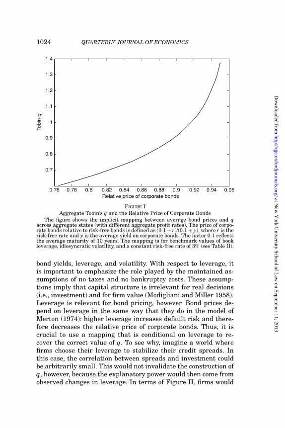
Figure I presents the main result. It shows the model-impliedaggregate q (s) as a function of the model-implied average relativebond price (φ + r) / (φ + y (s)). Figure I is generated by consideringall the possible values of the aggregate state variable s. Tobin’s q isan increasing and convex function of the relative price of corporatebonds. Figure I therefore extends Proposition 2 to the case oflong-term debt, persistent firm-level shocks, and large aggregateshocks.
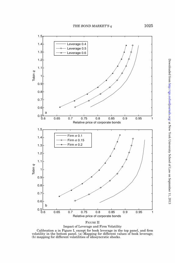
The mapping from bond yields to Tobin’s q is conditional onthe calibrated parameters, in particular on book leverage and id-iosyncratic volatility. Figure II shows the comparative statics withrespect to book leverage (ψ) and firm volatility (ση). The compar-ative statics is intuitive. For a given value of q, an increase inleverage leads to more credit risk and lower bond prices, so themapping shifts left when leverage increases. Similarly, for a givenvalue of q, an increase in idiosyncratic volatility increases creditrisk, and the mapping shifts left when volatility increases. In thiscase, the slope and the curvature of the mapping also change,and the intuition is given by Proposition 2: idiosyncratic volatilityincreases the delta of the bond with respect to q.
In the next section, mappings like the ones displayed inFigure II are used to construct a new measure of q from observed
at New
York U
niversity School of Law
on September 11, 2013
http://qje.oxfordjournals.org/D
ownloaded from
1024 QUARTERLY JOURNAL OF ECONOMICS
0.9
1
1.1
1.2
1.3
1.4
Tobin
q
0.76 0.78 0.8 0.82 0.84 0.86 0.88 0.9 0.92 0.94 0.96
0.7
0.8
Relative price of corporate bonds
FIGURE IAggregate Tobin’s q and the Relative Price of Corporate Bonds
The figure shows the implicit mapping between average bond prices and qacross aggregate states (with different aggregate profit rates). The price of corpo-rate bonds relative to risk-free bonds is defined as (0.1 + r)/(0.1 + y), where r is therisk-free rate and y is the average yield on corporate bonds. The factor 0.1 reflectsthe average maturity of 10 years. The mapping is for benchmark values of bookleverage, idiosyncratic volatility, and a constant risk-free rate of 3% (see Table II).
bond yields, leverage, and volatility. With respect to leverage, itis important to emphasize the role played by the maintained as-sumptions of no taxes and no bankruptcy costs. These assump-tions imply that capital structure is irrelevant for real decisions(i.e., investment) and for firm value (Modigliani and Miller 1958).Leverage is relevant for bond pricing, however. Bond prices de-pend on leverage in the same way that they do in the model ofMerton (1974): higher leverage increases default risk and there-fore decreases the relative price of corporate bonds. Thus, it iscrucial to use a mapping that is conditional on leverage to re-cover the correct value of q. To see why, imagine a world wherefirms choose their leverage to stabilize their credit spreads. Inthis case, the correlation between spreads and investment couldbe arbitrarily small. This would not invalidate the construction ofq, however, because the explanatory power would then come fromobserved changes in leverage. In terms of Figure II, firms would
at New
York U
niversity School of Law
on September 11, 2013
http://qje.oxfordjournals.org/D
ownloaded from
THE BOND MARKET’S q 1025
0.6 0.65 0.7 0.75 0.8 0.85 0.9 0.95 10.5
0.6
0.7
0.8
0.9
1
1.1
1.2
1.3
1.4
1.5To
bin
q
Relative price of corporate bonds
Leverage 0.4
Leverage 0.5
Leverage 0.6
0.6 0.65 0.7 0.75 0.8 0.85 0.9 0.95 10.5
0.6
0.7
0.8
0.9
1
1.1
1.2
1.3
1.4
1.5
Tobin
q
Relative price of corporate bonds
Firm σ 0.1
Firm σ 0.15
Firm σ 0.2
a
b
FIGURE IIImpact of Leverage and Firm Volatility
Calibration a in Figure I, except for book leverage in the top panel, and firmvolatility in the bottom panel. (a) Mapping for different values of book leverage;(b) mapping for different volatilities of idiosyncratic shocks.
at New
York U
niversity School of Law
on September 11, 2013
http://qje.oxfordjournals.org/D
ownloaded from
1026 QUARTERLY JOURNAL OF ECONOMICS
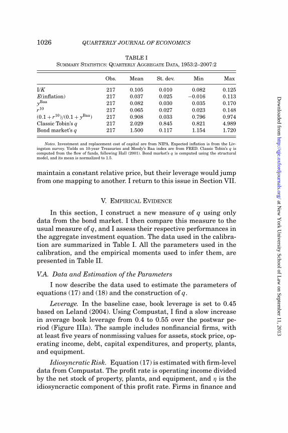
TABLE ISUMMARY STATISTICS: QUARTERLY AGGREGATE DATA, 1953:2–2007:2
Obs. Mean St. dev. Min Max
I/K 217 0.105 0.010 0.082 0.125E(inflation) 217 0.037 0.025 −0.016 0.113yBaa 217 0.082 0.030 0.035 0.170r10 217 0.065 0.027 0.023 0.148(0.1 + r10)/(0.1 + yBaa) 217 0.908 0.033 0.796 0.974Classic Tobin’s q 217 2.029 0.845 0.821 4.989Bond market’s q 217 1.500 0.117 1.154 1.720
Notes. Investment and replacement cost of capital are from NIPA. Expected inflation is from the Liv-ingston survey. Yields on 10-year Treasuries and Moody’s Baa index are from FRED. Classic Tobin’s q iscomputed from the flow of funds, following Hall (2001). Bond market’s q is computed using the structuralmodel, and its mean is normalized to 1.5.
maintain a constant relative price, but their leverage would jumpfrom one mapping to another. I return to this issue in Section VII.
V. EMPIRICAL EVIDENCE
In this section, I construct a new measure of q using onlydata from the bond market. I then compare this measure to theusual measure of q, and I assess their respective performances inthe aggregate investment equation. The data used in the calibra-tion are summarized in Table I. All the parameters used in thecalibration, and the empirical moments used to infer them, arepresented in Table II.
V.A. Data and Estimation of the Parameters
I now describe the data used to estimate the parameters ofequations (17) and (18) and the construction of q.
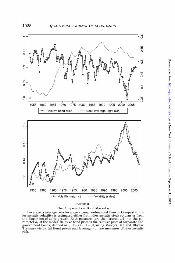
Leverage. In the baseline case, book leverage is set to 0.45based on Leland (2004). Using Compustat, I find a slow increasein average book leverage from 0.4 to 0.55 over the postwar pe-riod (Figure IIIa). The sample includes nonfinancial firms, withat least five years of nonmissing values for assets, stock price, op-erating income, debt, capital expenditures, and property, plants,and equipment.
Idiosyncratic Risk. Equation (17) is estimated with firm-leveldata from Compustat. The profit rate is operating income dividedby the net stock of property, plants, and equipment, and η is theidiosyncractic component of this profit rate. Firms in finance and
at New
York U
niversity School of Law
on September 11, 2013
http://qje.oxfordjournals.org/D
ownloaded from
THE BOND MARKET’S q 1027
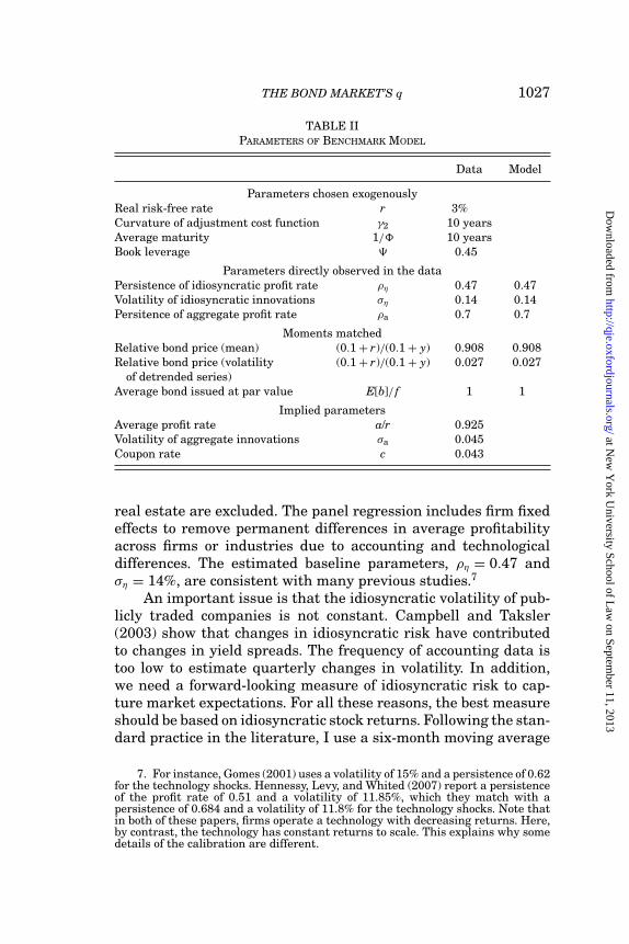
TABLE IIPARAMETERS OF BENCHMARK MODEL
Data Model
Parameters chosen exogenouslyReal risk-free rate r 3%Curvature of adjustment cost function γ2 10 yearsAverage maturity 1/� 10 yearsBook leverage 0.45
Parameters directly observed in the dataPersistence of idiosyncratic profit rate ρη 0.47 0.47Volatility of idiosyncratic innovations ση 0.14 0.14Persitence of aggregate profit rate ρa 0.7 0.7
Moments matchedRelative bond price (mean) (0.1 + r)/(0.1 + y) 0.908 0.908Relative bond price (volatility (0.1 + r)/(0.1 + y) 0.027 0.027
of detrended series)Average bond issued at par value E[b]/ f 1 1
Implied parametersAverage profit rate a/r 0.925Volatility of aggregate innovations σa 0.045Coupon rate c 0.043
real estate are excluded. The panel regression includes firm fixedeffects to remove permanent differences in average profitabilityacross firms or industries due to accounting and technologicaldifferences. The estimated baseline parameters, ρη = 0.47 andση = 14%, are consistent with many previous studies.7
An important issue is that the idiosyncratic volatility of pub-licly traded companies is not constant. Campbell and Taksler(2003) show that changes in idiosyncratic risk have contributedto changes in yield spreads. The frequency of accounting data istoo low to estimate quarterly changes in volatility. In addition,we need a forward-looking measure of idiosyncratic risk to cap-ture market expectations. For all these reasons, the best measureshould be based on idiosyncratic stock returns. Following the stan-dard practice in the literature, I use a six-month moving average
7. For instance, Gomes (2001) uses a volatility of 15% and a persistence of 0.62for the technology shocks. Hennessy, Levy, and Whited (2007) report a persistenceof the profit rate of 0.51 and a volatility of 11.85%, which they match with apersistence of 0.684 and a volatility of 11.8% for the technology shocks. Note thatin both of these papers, firms operate a technology with decreasing returns. Here,by contrast, the technology has constant returns to scale. This explains why somedetails of the calibration are different.
at New
York U
niversity School of Law
on September 11, 2013
http://qje.oxfordjournals.org/D
ownloaded from
1028 QUARTERLY JOURNAL OF ECONOMICS
0.3
50.4
0.4
50.5
0.5
50.6
0.8
0.8
50.9
0.9
51
1955 1960 1965 1970 1975 1980 1985 1990 1995 2000 2005
Relative bond price Book leverage (right axis)
0.1
20.1
40.1
60.1
8
1955 1960 1965 1970 1975 1980 1985 1990 1995 2000 2005
Volatility (returns) Volatility (sales)
a
b
FIGURE IIIThe Components of Bond Market q
Leverage is average book leverage among nonfinancial firms in Compustat. Id-iosyncratic volatility is estimated either from idiosyncratic stock returns or fromthe dispersion of sales growth. Both measures are then translated into the pa-rameter ση of the model. Relative bond price is the relative price of corporate andgovernment bonds, defined as (0.1 + r)/(0.1 + y), using Moody’s Baa and 10-yearTreasury yields. (a) Bond prices and leverage; (b) two measures of idiosyncraticrisk.
at New
York U
niversity School of Law
on September 11, 2013
http://qje.oxfordjournals.org/D
ownloaded from
THE BOND MARKET’S q 1029
of the monthly cross-sectional standard deviation of individualstock returns. I scale this new measure to have a sample mean of14% to obtain σ
ηt , a time-varying estimate of idiosyncratic risk. As
a robustness check, I also consider the cross-sectional standarddeviation of the growth rate of sales, measured from Compustat,as a measure of volatility that avoids using stock returns.8 Thetwo measures of σ
ηt are presented in Figure IIIb.
Aggregate Bond Prices. Moody’s Baa index, denoted yBaat ,
is the main measure of the yield on risky corporate debt. Moody’sindex is the equal weighted average of yields on Baa-rated bondsissued by large nonfinancial corporations.9 Following the litera-ture, the 10-year treasury yield is used as the benchmark risk-freerate. Both r10
t and yBaat are obtained from FRED.10
For equation (18), using annual NIPA data on corporate prof-its and the stock of nonresidential capital over the postwar period,I estimate ρa = 0.7. The parameters a and σa cannot be cali-brated with historical aggregate profit rates because they mustcapture risk-adjusted values, not historical ones.11 Instead, themodel must be consistent with observed bond prices. Three pa-rameters are thus not directly observed in the data: these are c(the coupon rate), a, and σa. Their values are inferred by match-ing empirical and simulated moments. The empirical momentsare the mean and standard deviation of the price of Baa bonds
8. The dispersion of sales growth is not a perfect measure either, becausepermanent differences in growth rates would make dispersion positive even ifthere is no risk. There are other ways to define idiosyncratic risk at the firm level,but they produce similar trends. See Comin and Philippon (2005) for a comparisonof various measures of firm volatility. See also Campbell et al. (2001) and Daviset al. (2006) for evidence on privately held companies.
9. To be included in the index, a bond must have a face value of at least 100million, an initial maturity of at least 20 years, and most importantly, a liquidsecondary market. Beyond these characteristics, Moody’s has some discretion onthe selection of the bonds. The number of bonds included in the index varies from75 to 100 in any given year. The main advantages of Moody’s measure are that it isavailable since 1919, and that it is broadly representative of the U.S. nonfinancialsector, because Baa is close to the median among rated companies.
10. Federal Reserve Economic Data: http://research.stlouisfed.org/fred2/. Theissue with using the ten-year treasury bond is that it incorporates a liquiditypremium relative to corporate bonds. To adjust for this, it is customary to usethe LIBOR/swap rate instead of the treasury rate as a measure of risk-free rate(see Duffie and Singleton [2003] and Lando [2004]), but these rates are only avail-able for relatively recent years. I add 30 basis points to the risk-free rate to adjustfor liquidity (see Almeida and Philippon [2007] for a discussion of this issue).
11. Note that, in theory, the same applies to ρa, because persistence underthe risk-neutral measure can be different from persistence under the physicalmeasure. In practice, however, the difference for ρa is much smaller than for a orσa. I therefore take the historical persistence to be a good approximation of therisk neutral persistence. Section VII shows that the model is robust to variousassumptions regarding aggregate dynamics.
at New
York U
niversity School of Law
on September 11, 2013
http://qje.oxfordjournals.org/D
ownloaded from
1030 QUARTERLY JOURNAL OF ECONOMICS
relative to Treasuries, defined as (φ + r$t )/(φ + y$
t ), where y$ is theyield on Baa corporate bonds and r$ is the yield on governmentbonds. The final requirement is that the average bond be issuedat par. The three parameters c, a, and σa are chosen simultane-ously to match the par-value requirement and the two empiricalmoments. The parameters inferred from the simulated momentsare c = 4.3%, a/r = 0.925, and σa = 4.5%.
Expected Inflation and Real Rate. The Livingston survey isused to construct expected inflation, and the yield on the ten-yeartreasury to construct the ex ante real interest rate, rreal
t .
Creating qbond. The model described in Section IV constructsq from the relative price of corporate bonds, conditional on thebaseline values for the risk-free rate, book leverage, and idiosyn-cratic risk. As I have just explained, the risk-free rate, book lever-age, and idiosyncratic volatility move over time. Therefore, qbond
is a function of four observed inputs: average book leverage ψt,average idiosyncratic volatility σ
ηt , the ex ante real rate rreal
t , andthe relative price of corporate bonds
qbondt = F
(φ + r10
t
φ + yBaat
; σ ηt ; ψt; rreal
t
).(19)
Figure III displays the three main components: leverage, volatil-ity, and the relative price. In theory, the dynamics of the fourinputs must be jointly specified to construct the mapping ofequation (19). Quantitatively, however, it turns out that one canestimate mappings with respect to (φ + r10
t )/(φ + yBaat ) assuming
constant values for the other three parameters, as I did in Fig-ure II. For the risk-free rate, this follows from a well-known fact inthe bond pricing literature: risk-free rate dynamics plays a negli-gible role in fitting corporate spreads. For σ
ηt and ψt, the historical
series are so persistent that there is little difference between themapping assuming a constant value and the mapping conditionalon the same value in the time-varying model.12
Classic Measure of Tobin’s q. The usual measure of Tobin’s qis constructed from the flow of funds as in Hall (2001). The usual
12. To check this, I construct an extended Markov model where all the pa-rameters follow AR(1) processes calibrated from the data. I then create mappingsconditional on each realization of the parameters and I compare them to the map-pings from Figure II. I find that the discrepancies are small for volatility andinvisible for book leverage and the risk-free rate. Detailed results and figures areavailable upon request.
at New
York U
niversity School of Law
on September 11, 2013
http://qje.oxfordjournals.org/D
ownloaded from
THE BOND MARKET’S q 1031
34
51
2
1955 1960 1965 1970 1975 1980 1985 1990 1995 2000 2005
Usual q Bond q
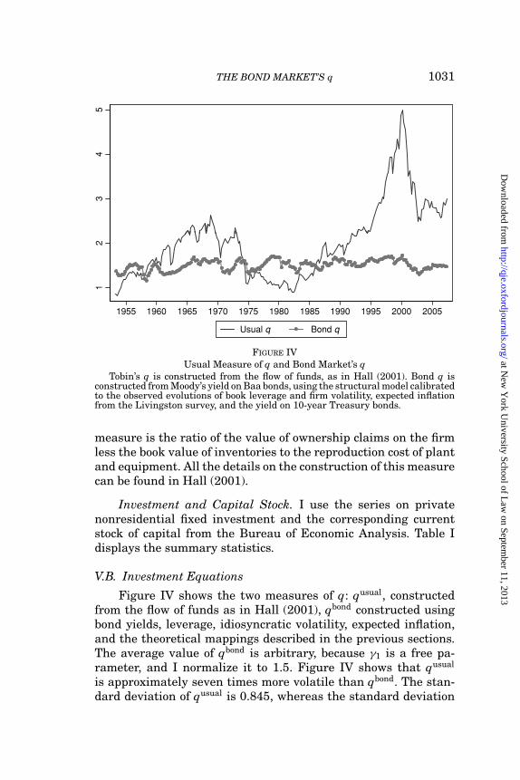
FIGURE IVUsual Measure of q and Bond Market’s q
Tobin’s q is constructed from the flow of funds, as in Hall (2001). Bond q isconstructed from Moody’s yield on Baa bonds, using the structural model calibratedto the observed evolutions of book leverage and firm volatility, expected inflationfrom the Livingston survey, and the yield on 10-year Treasury bonds.
measure is the ratio of the value of ownership claims on the firmless the book value of inventories to the reproduction cost of plantand equipment. All the details on the construction of this measurecan be found in Hall (2001).
Investment and Capital Stock. I use the series on privatenonresidential fixed investment and the corresponding currentstock of capital from the Bureau of Economic Analysis. Table Idisplays the summary statistics.
V.B. Investment Equations
Figure IV shows the two measures of q: qusual, constructedfrom the flow of funds as in Hall (2001), qbond constructed usingbond yields, leverage, idiosyncratic volatility, expected inflation,and the theoretical mappings described in the previous sections.The average value of qbond is arbitrary, because γ1 is a free pa-rameter, and I normalize it to 1.5. Figure IV shows that qusual
is approximately seven times more volatile than qbond. The stan-dard deviation of qusual is 0.845, whereas the standard deviation
at New
York U
niversity School of Law
on September 11, 2013
http://qje.oxfordjournals.org/D
ownloaded from
1032 QUARTERLY JOURNAL OF ECONOMICS
34
5q
0.1
0.1
10
.12
0.1
3I/
K
12
0.0
80
.09
1955 1960 1965 1970 1975 1980 1985 1990 1995 2000 2005
I/K Usual q
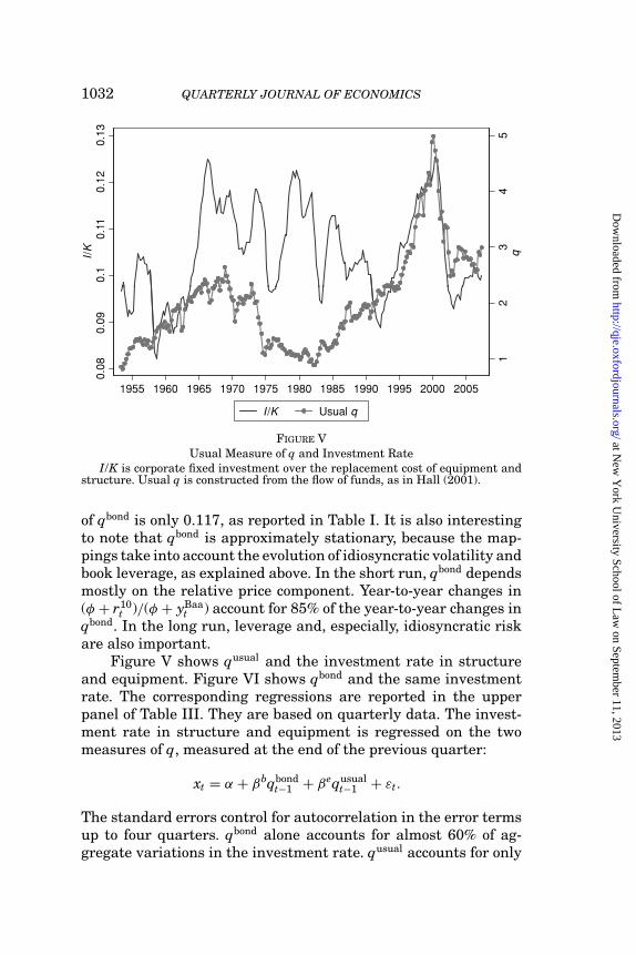
FIGURE VUsual Measure of q and Investment Rate
I/K is corporate fixed investment over the replacement cost of equipment andstructure. Usual q is constructed from the flow of funds, as in Hall (2001).
of qbond is only 0.117, as reported in Table I. It is also interestingto note that qbond is approximately stationary, because the map-pings take into account the evolution of idiosyncratic volatility andbook leverage, as explained above. In the short run, qbond dependsmostly on the relative price component. Year-to-year changes in(φ + r10
t )/(φ + yBaat ) account for 85% of the year-to-year changes in
qbond. In the long run, leverage and, especially, idiosyncratic riskare also important.
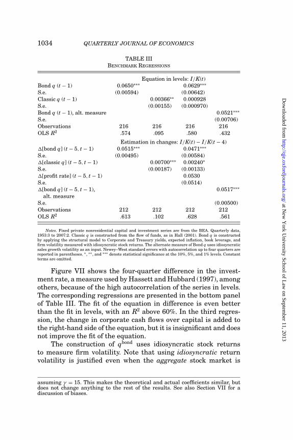
Figure V shows qusual and the investment rate in structureand equipment. Figure VI shows qbond and the same investmentrate. The corresponding regressions are reported in the upperpanel of Table III. They are based on quarterly data. The invest-ment rate in structure and equipment is regressed on the twomeasures of q, measured at the end of the previous quarter:
xt = α + βbqbondt−1 + βequsual
t−1 + εt.
The standard errors control for autocorrelation in the error termsup to four quarters. qbond alone accounts for almost 60% of ag-gregate variations in the investment rate. qusual accounts for only
at New
York U
niversity School of Law
on September 11, 2013
http://qje.oxfordjournals.org/D
ownloaded from
THE BOND MARKET’S q 1033
1.4
1.5
1.6
1.7
1.8
Bo
nd
q
0.1
0.1
10
.12
0.1
3I/
K
1.1
1.2
1.3
0.0
80
.09
1955 1960 1965 1970 1975 1980 1985 1990 1995 2000 2005
I/K Bond q
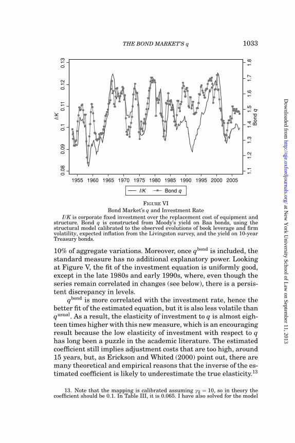
FIGURE VIBond Market’s q and Investment Rate
I/K is corporate fixed investment over the replacement cost of equipment andstructure. Bond q is constructed from Moody’s yield on Baa bonds, using thestructural model calibrated to the observed evolutions of book leverage and firmvolatility, expected inflation from the Livingston survey, and the yield on 10-yearTreasury bonds.
10% of aggregate variations. Moreover, once qbond is included, thestandard measure has no additional explanatory power. Lookingat Figure V, the fit of the investment equation is uniformly good,except in the late 1980s and early 1990s, where, even though theseries remain correlated in changes (see below), there is a persis-tent discrepancy in levels.
qbond is more correlated with the investment rate, hence thebetter fit of the estimated equation, but it is also less volatile thanqusual. As a result, the elasticity of investment to q is almost eigh-teen times higher with this new measure, which is an encouragingresult because the low elasticity of investment with respect to qhas long been a puzzle in the academic literature. The estimatedcoefficient still implies adjustment costs that are too high, around15 years, but, as Erickson and Whited (2000) point out, there aremany theoretical and empirical reasons that the inverse of the es-timated coefficient is likely to underestimate the true elasticity.13
13. Note that the mapping is calibrated assuming γ2 = 10, so in theory thecoefficient should be 0.1. In Table III, it is 0.065. I have also solved for the model
at New
York U
niversity School of Law
on September 11, 2013
http://qje.oxfordjournals.org/D
ownloaded from
1034 QUARTERLY JOURNAL OF ECONOMICS
TABLE IIIBENCHMARK REGRESSIONS
Equation in levels: I/K(t)Bond q (t − 1) 0.0650∗∗∗ 0.0629∗∗∗S.e. (0.00594) (0.00642)Classic q (t − 1) 0.00366∗∗ 0.000928S.e. (0.00155) (0.000970)Bond q (t − 1), alt. measure 0.0521∗∗∗S.e. (0.00706)Observations 216 216 216 216OLS R2 .574 .095 .580 .432
Estimation in changes: I/K(t) − I/K(t − 4)�[bond q] (t − 5, t − 1) 0.0515∗∗∗ 0.0471∗∗∗S.e. (0.00495) (0.00584)�[classic q] (t − 5, t − 1) 0.00700∗∗∗ 0.00240∗S.e. (0.00187) (0.00133)�[profit rate] (t − 5, t − 1) 0.0530S.e. (0.0514)�[bond q] (t − 5, t − 1), 0.0517∗∗∗
alt. measureS.e. (0.00500)Observations 212 212 212 212OLS R2 .613 .102 .628 .561
Notes. Fixed private nonresidential capital and investment series are from the BEA. Quarterly data,1953:3 to 2007:2. Classic q is constructed from the flow of funds, as in Hall (2001). Bond q is constructedby applying the structural model to Corporate and Treasury yields, expected inflation, book leverage, andfirm volatility measured with idiosyncratic stock returns. The alternate measure of Bond q uses idiosyncraticsales growth volatility as an input. Newey–West standard errors with autocorrelation up to four quarters arereported in parentheses. ∗ , ∗∗ , and ∗∗∗ denote statistical significance at the 10%, 5%, and 1% levels. Constantterms are omitted.
Figure VII shows the four-quarter difference in the invest-ment rate, a measure used by Hassett and Hubbard (1997), amongothers, because of the high autocorrelation of the series in levels.The corresponding regressions are presented in the bottom panelof Table III. The fit of the equation in difference is even betterthan the fit in levels, with an R2 above 60%. In the third regres-sion, the change in corporate cash flows over capital is added tothe right-hand side of the equation, but it is insignificant and doesnot improve the fit of the equation.
The construction of qbond uses idiosyncratic stock returnsto measure firm volatility. Note that using idiosyncratic returnvolatility is justified even when the aggregate stock market is
assuming γ = 15. This makes the theoretical and actual coefficients similar, butdoes not change anything to the rest of the results. See also Section VII for adiscussion of biases.
at New
York U
niversity School of Law
on September 11, 2013
http://qje.oxfordjournals.org/D
ownloaded from

THE BOND MARKET’S q 1035
00.0
10.0
2–
0.0
2–
0.0
1
1955 1960 1965 1970 1975 1980 1985 1990 1995 2000 2005time
Change in I /K from t –4 to t Predicted with lagged bond q
FIGURE VIIFour-Quarter Changes in Investment Rate, Actual and Predicted
I/K is corporate fixed investment over the replacement cost of equipment andstructure. Bond q is constructed from Moody’s yield on Baa bonds, using thestructural model calibrated to the observed evolutions of book leverage and firmvolatility, expected inflation from the Livingston survey, and the yield on 10-yearTreasury bonds.
potentially mispriced. Mispricing across firms is limited by thepossibility of arbitrage. In the aggregate, however, arbitrage ismuch more difficult. There is therefore no inconsistency in usingthe idiosyncratic component of stock returns to measure idiosyn-cratic risk, although acknowledging that the aggregate stockmarket can sometimes be over valued.
Nonetheless, one might be concerned about the use of eq-uity returns here, and I have repeated the calibration usingthe standard deviation of sales growth as a measure of volatil-ity. The results, in the last column of Table III, are somewhatweaker than with the benchmark model. The reason is that salesvolatility is a lagging indicator of idiosyncratic risk. Hilscher(2007) shows that the bond market is actually forward-lookingfor volatility. As a result, using a measure of volatility thatlags the true information—and all accounting measures do—creates a specification error. This matters less for the equa-tion in changes because of the smaller role of volatility in thatequation.
at New
York U
niversity School of Law
on September 11, 2013
http://qje.oxfordjournals.org/D
ownloaded from
1036 QUARTERLY JOURNAL OF ECONOMICS
The conclusions from this empirical section are the following:• With aggregate U.S. data, qbond fits the investment equation
well, both in levels and in differences.• The estimated elasticity of investment to qbond is 18 times
higher than the one estimated with qusual.• Corporate cash flows do not have significant explanatory
power once qbond is included in the regression.
V.C. Further Evidence
The evidence presented above is based on the construction ofqbond in equation (19). In this section, I provide evidence on theexplanatory power of the components separately, and on the roleof nonlinearities in the model. I also test the predictive power ofthe model. The results are in Tables IV and V.
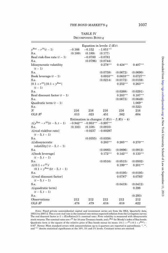
Explanatory Power of Individual Components. The econo-metric literature has studied the predictive power of defaultspreads for real economic activity.14 Table IV shows the explana-tory power of the components of qbond, in levels and in four-quarterdifferences.
Consider first the top part of Table IV, for the regressions inlevel. Column (1) shows that the Baa spread, by itself, has no ex-planatory power for investment. The explanatory power appearsonly when idiosyncratic volatility and leverage are also included,in Column (3). These factors have not been used in the empiricalliterature. Their empirical importance provides support for thetheory developed in this paper.
In addition, notice that even when all the components areentered linearly, the explanatory power is only 45%. By contrast,the qbond has an R2 of 57.4% with one degree of freedom instead offour. This shows that the nonlinearities are important in the levelequation, as explained below.
For the equation in four-quarter differences, the spread by it-self has significant explanatory power. This is what one wouldexpect, because the low-frequency movements in leverage andvolatility matter less in these regressions. Nonetheless, leverageand volatility are still highly significant. The unrestricted linear
14. Bernanke (1983) notes that the spread of Baa over treasury went “from 2.5percent during 1929–30 to nearly 8 percent in the mid-1932” and shows that thespread was a useful predictor of industrial production growth. Using monthly datafrom 1959 to 1988, Stock and Watson (1989) find that the spread between commer-cial paper and Treasury bills predicts output growth. Some of these relationshipsare unstable over time (see Stock and Watson [2003] for a survey).
at New
York U
niversity School of Law
on September 11, 2013
http://qje.oxfordjournals.org/D
ownloaded from
THE BOND MARKET’S q 1037
TABLE IVDECOMPOSING BOND q
Equation in levels: I/K(t)yBaa − r10(t − 1) −0.166 −0.152 −1.051∗∗∗
S.e. (0.189) (0.189) (0.177)Real risk-free rate (t − 1) −0.0700 −0.0781S.e. (0.0796) (0.0744)Idiosyncratic volatility 0.278∗∗∗ 0.424∗∗∗ 0.407∗∗∗
(t − 1)S.e. (0.0759) (0.0672) (0.0690)Book leverage (t − 1) 0.0910∗∗∗ 0.0633∗∗∗ 0.0727∗∗∗
S.e. (0.0214) (0.0172) (0.0159)[0.1 + r10]/[0.1 + yBaa] 0.252∗∗∗ 0.263∗∗∗
(t − 1)S.e. (0.0268) (0.0291)Real discount factor (t − 1) 0.203∗∗∗ 0.187∗∗∗
S.e. (0.0673) (0.0649)Quadratic term (t − 1) 1.069∗∗
S.e. (0.522)N 216 216 216 216 216OLS R2 .013 .023 .451 .582 .604
Estimation in changes: I/K(t) − I/K(t − 4)�[yBaa − r10](t − 5, t − 1) −0.942∗∗∗ −0.953∗∗∗ −0.997∗∗∗
S.e. (0.103) (0.108) (0.0910)�[real riskfree rate] −0.0237 −0.00297
(t − 5, t − 1)S.e. (0.0355) (0.0338)�[idiosyncratic 0.283∗∗∗ 0.265∗∗∗ 0.270∗∗∗
volatility] (t − 5, t − 1)S.e. (0.0885) (0.0896) (0.0912)�[book leverage] 0.172∗∗∗ 0.142∗∗∗ 0.133∗∗∗
(t − 5, t − 1)S.e. (0.0516) (0.0515) (0.0502)�[(0.1 + r10)/ 0.199∗∗∗ 0.201∗∗∗
(0.1 + yBaa)](t − 5, t − 1)S.e. (0.0195) (0.0195)�[real discount factor] 0.0787∗ 0.0765∗
(t − 5, t − 1)S.e. (0.0419) (0.0412)�[quadratic term] 0.398
(t − 5, t − 1)S.e. (0.293)Observations 212 212 212 212 212OLS R2 .478 .479 .618 .618 .622
Notes. Fixed private nonresidential capital and investment series are from the BEA. Quarterly data,1953:3 to 2007:2. The ex ante real rate is the nominal rate minus expected inflation from the Livingston survey.The real discount factor is (1 + E[inflation])/(1+nominal rate). Firm volatility is measured with idiosyncraticstock returns. The nominal rates are r10 for 10-year Treasury bonds, and yBaa for Moody’s index of Baa bonds.Quadratic term is the square of the relative price of Baa bonds minus its mean: [(0.1 + r10)/(0.1 + yBaa) −0.9]2. Newey–West standard errors with autocorrelation up to 4 quarters are reported in parentheses. ∗, ∗∗ ,and ∗∗∗ denote statistical significance at the 10%, 5% and 1% levels. Constant terms are omitted.
at New
York U
niversity School of Law
on September 11, 2013
http://qje.oxfordjournals.org/D
ownloaded from
1038 QUARTERLY JOURNAL OF ECONOMICS
TA
BL
EV
PR
ED
ICT
IVE
RE
GR
ES
SIO
NS,
ON
EQ
UA
RT
ER
AH
EA
D:M
AX
IMU
ML
IKE
LIH
OO
DE
ST
IMA
TIO
NO
FA
UT
OR
EG
RE
SS
IVE
MO
DE
L
Gro
wth
rate
ofG
row
thra
teof
Gro
wth
rate
ofpr
ivat
en
onre
side
nti
alfi
xed
inve
stm
ent
con
sum
ptio
nre
side
nti
alin
vest
men
t
�[b
ond
q](t
−1)
0.14
8∗∗∗
0.16
0∗∗∗
0.16
1∗∗∗
0.01
190.
0279
S.e.
(0.0
231)
(0.0
251)
(0.0
247)
(0.0
0917
)(0
.041
7)�
log[
real
GD
P]
(t−
1)0.
710∗
∗∗0.
760∗
∗∗0.
797∗
∗∗0.
169∗
∗∗−0
.162
S.e.
(0.1
82)
(0.1
99)
(0.2
00)
(0.0
585)
(0.3
46)
�[c
lass
icQ
](t
−1)
0.01
300.
0097
6∗∗∗
0.04
01∗∗
S.e.
(0.0
0955
)(0
.002
79)
(0.0
184)
AR
(1)
0.39
6∗∗∗
0.33
7∗∗∗
0.13
10.
0996
0.02
060.
511∗
∗∗S.
e.(0
.077
8)(0
.083
2)(0
.093
5)(0
.092
8)(0
.083
2)(0
.054
3)O
bser
vati
ons
215
215
215
215
215
215
R2
ofO
LS
.398
.341
.430
.443
.149
.335
Not
es.M
axim
um
like
lih
ood
esti
mat
ion
ofco
effi
cien
tsan
dst
anda
rder
rors
,ass
um
ing
AR
(1)m
odel
.Th
eR
2is
for
the
corr
espo
ndi
ng
OL
Sre
gres
sion
wit
hla
gged
depe
nde
nt
vari
able
onth
eri
ght-
han
dsi
de.F
ixed
priv
ate
non
resi
den
tial
inve
stm
ent
seri
esis
from
the
BE
A.Q
uar
terl
yda
ta,1
953:
3to
2007
:2.B
ond
qis
con
stru
cted
byap
plyi
ng
the
stru
ctu
ral
mod
elto
Cor
pora
tean
dT
reas
ury
yiel
ds,e
xpec
ted
infl
atio
n,b
ook
leve
rage
,an
dfi
rmvo
lati
lity
mea
sure
dw
ith
idio
syn
crat
icst
ock
retu
rns.
Con
stan
tte
rms
are
omit
ted.
at New
York U
niversity School of Law
on September 11, 2013
http://qje.oxfordjournals.org/D
ownloaded from
THE BOND MARKET’S q 1039
model has an R2 of 61.6%, compared to 61.3% for the bond qmodel. This suggests that, also as expected, nonlinear effects arenot crucial for the specification in changes.
Nonlinear Effects. There are several nonlinear effects in themodel. Consider equation (4): Tobin’s q has two components, thereal discount factor and the expected risk-neutral value of capital,Eπ [v(ω′)|ω]. This letter item is a function of the relative price ofcorporate bonds, as shown in Figures I and II. Thus, the modelsuggests the use of the relative price (φ + r10
t )/(φ + yBaat ) instead
of the spread yBaat − r10
t . When rates are stable, the differencebetween the spread and the relative price is negligible. In thedata, however, the level of nominal rates changes a lot. A givenchange in the spread has a larger impact on the relative pricewhen rates are low than when they are high.
Column (4) provides strong support for this first nonlinearity.The relative price does much better than the spread in the levelregression.15 The R2 increases from 45.1% to 58.2% because of thenonlinear correction.
A second nonlinearity comes from the mapping of Figure I.Tobin’s q is a convex function of the relative bond price. Column(5) shows that this effect is significant, but it only increases theR2 by 2 percentage points.
The last column of Table IV can also be compared to the firstcolumn of Table III. In level, the structural model has a fit of57.4%. The unrestricted nonlinear model has a fit of 60.4%. In astatistical sense, the difference is significant, but in an economicsense, it does not appear very important. In differences, the re-spective performances are 61.3% and 62.2%. These results supportthe restrictions imposed by the theory.
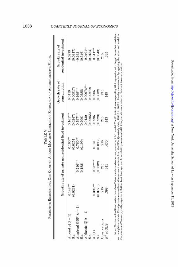
Predictive Regressions. Table V reports the results from pre-dictive regressions of the growth rate of three macroeconomic vari-ables: real corporate investment, real consumption expenditures,and real residential investment. In each case, I run two separateregressions. I estimate an AR(1) model by maximum likelihood toobtain the correct coefficients and standard errors. I also run anOLS regression with the lagged dependent variable on the RHSto get a sense of the R2 of the simple linear regression.
15. Note that, in theory, this could also apply to the real discount factor:(1 + E[inflation])/(1 + r$) is not the same as E[inflation] − r$ when nominal shocksare large. Empirically, this nonlinearity seems to matter much less, probably be-cause the real rate is not as volatile as the Baa yield.
at New
York U
niversity School of Law
on September 11, 2013
http://qje.oxfordjournals.org/D
ownloaded from

1040 QUARTERLY JOURNAL OF ECONOMICS
The first column shows that qbond is a very significant pre-dictor of corporate investment growth. It predicts better than the“accelerator” model based on lagged output growth (column (2)).While lagged output growth still has significant marginal fore-casting power, it increases the R2 by only 3 percentage points(column (3)). In addition, the coefficient on qbond actually goes up.Column (4) shows that qusual has no predictive power for corporateinvestment.16
The last two columns focus on consumption and residentialinvestment. Although qbond is the best predictor of corporate in-vestment, it does not predict housing or consumption. qusual, on theother hand, does not predict corporate investment, but it does pre-dict housing and (to some extent) consumption. These results aresuggestive of wealth effects from the equity market. They are con-sistent with the results of Hassett and Hubbard (1997) but clearlyinconsistent with the usual implementation of the q-theory.
The conclusions from this empirical section are the following:• All the components identified by the theory (bond spreads,
volatility, leverage, risk-free rate) are statistically and eco-nomically significant.
• The fit of the restricted structural model is almost as goodas the fit of the unrestricted regressions.
• The nonlinearities of the model (relative price instead ofspreads, convexity of mapping) are important for the levelregressions.
• The bond market predicts future corporate investment well,whereas the equity market has no marginal predictivepower.
VI. THEORETICAL EXPLANATIONS
The results so far show that it is possible to link corporateinvestment and asset prices, using the corporate bond marketand modern asset pricing theory. They do not explain why theusual approach fails, however. This section sheds some light onthis complex question.
16. Fama (1981) shows that stock prices have little forecasting power foroutput. Cochrane (1996) finds a significant correlation between stock returns andthe growth rate of the aggregate capital stock, but Hassett and Hubbard (1997)argue that it is driven by the correlation with residential investment, not corporateinvestment. In any case, I find that the bond market’s q outperforms the usualmeasure both in differences and in levels.
at New
York U
niversity School of Law
on September 11, 2013
http://qje.oxfordjournals.org/D
ownloaded from
THE BOND MARKET’S q 1041
It is important to recognize that a satisfactory explanationmust address two related but distinct issues:
1. Why is qusual more volatile than qbond?2. Why does qbond fit the investment equation better?I consider two explanations.17 The first explanation is based
on growth options and the distinction between average andmarginal q. The second explanation is based on mispricing in theequity market. I chose these explanations because they provideuseful benchmarks. They are not mutually exclusive, and theyare not the only possible explanations.
VI.A. Growth Option Interpretation
Suppose that, in addition to the value process in equation (3),the firm also has a growth option of value Gt. Total firm value isthen
Vt = vtkt−1 + Gt.(20)
Consider for simplicity the example of Section III, with short-termdebt and a constant risk-free rate. The value of short-term debt is
Bt = 11 + r
Eπt [min(t; vt+1kt + Gt+1)].(21)
Let Gt be a binary variable. Gt = GH, with risk-neutral probabilityλt−1 and GL otherwise. The following proposition states that agrowth option with enough skewness can explain why qbond fitsbetter than qusual.
PROPOSITION 3. Consider the model of equations (20) and (21). Bychoosing λt and GL small enough, and GH large enough, the fitof the investment equation can be arbitrarily good for qbond,and arbitrarily poor for qusual.
Proof. See the Appendix.
The intuition behind Proposition 3 is straightforward. A smallprobability of a large positive shock has a large impact on eq-uity prices, and almost no impact on bond prices. Because growthoptions do not depend on the capital stock, news about the likeli-hood of these future shocks does not affect investment. In essence,
17. For a investigation of whether the same pricing kernel can price bondsand stocks, see Chen, Collin-Dufresne, and Goldstein (forthcoming).
at New
York U
niversity School of Law
on September 11, 2013
http://qje.oxfordjournals.org/D
ownloaded from
1042 QUARTERLY JOURNAL OF ECONOMICS
growth options drive wedges between bond and equity prices, andbetween marginal and average q.
What are the possible interpretations of these shocks? Thesimplest one is that firms earn organizational rents. Think of alarge industrial corporation with outstanding organizational cap-ital. This firm will be able to seize new opportunities if and whenthey arrive. This might happen through mergers and acquisitionsor through internal development of new lines of business. Invest-ing more in the current business and current technology does notimprove this option value.18
To summarize, the rational interpretation proposes the fol-lowing answers to the two questions posed at the beginning ofthis section:
1. Why is qusual more volatile than qbond? Because growthoptions affect stocks much more than bonds.
2. Why does qbond fit the investment equation better? Becausegrowth options are unrelated to current capital expendi-tures.
The example given is obviously extreme, but the lesson is ageneral one. It is not difficult to come up with a story where cur-rent capital expenditures are well explained by the bond market,whereas firm creation, IPOs, and perhaps R&D, are better ex-plained by the equity market. A complete understanding of thesejoint dynamics is an important topic for future research.
VI.B. Mispricing Interpretation
Stein (1996) analyzes capital budgeting in the presence ofsystematic pricing errors by investors, assuming that managershave rational expectations. He emphasizes three crucial aspectsof capital budgeting in such a world: (i) the true NPV of invest-ment, (ii) the gains from trading mispriced securities, and (iii) thecosts of deviating from an optimal capital structure in order toachieve (i) and (ii). For the purpose of my paper, the most impor-tant result is that when capital structure is not a constraint, andwhen managers have long horizons, real investment decisions arenot influenced by mispricing (Stein 1996, Proposition 3).
18. Some other expenditures could be complement with the option value.These could include R&D and reorganizations. At the aggregate level, one mightthink that new options were realized by new firms. This would explain why IPOsare correlated with the equity market (Jovanovic and Rousseau 2001). For a modelof growth option at the firm level, see Abel and Eberly (2005).
at New
York U
niversity School of Law
on September 11, 2013
http://qje.oxfordjournals.org/D
ownloaded from
THE BOND MARKET’S q 1043
Gilchrist, Himmelberg, and Huberman (2005) consider amodel where mispricing comes from heterogeneous beliefs andshort sales constraints. They show that increases in dispersionof investor opinion cause stock prices to rise above their funda-mental values. This leads to an increase in q, share issues, andreal investment. The main difference from Stein (1996) is thatthey assume that investors do not overvalue cash held in the firm.This assumption rules out the separation of real and financialdecisions: managers who seek to exploit mispricing must altertheir investment decisions and Proposition 3 in Stein (1996) doesnot hold. However, Gilchrist, Himmelberg, and Huberman (2005)show that even large pricing errors need not have large effectson investment. Thus, it is possible to explain the fact that invest-ment does not react much to equity mispricing, even when thestrict dichotomy of Stein (1996)’s Proposition 3 fails.
Neither Stein (1996) nor Gilchrist, Himmelberg, and Huber-man (2005) consider the role of bonds and stocks separately, so itappears that the story is still incomplete. It turns out, however,that recent work in behavioral finance has shown that skewedassets are more likely to be mispriced (Barberis and Huang 2007;Brunnermeier, Gollier, and Parker 2007; Mitton and Vorkink2007). A direct implication is that mispricing is more likely toappear in the equity market than in the bond market. Of course,mispricing can also happen in the bond market. Piazzesi andSchneider (2006), for instance, analyze the consequences for assetprices of disagreement about inflation expectations.
To summarize, the behavioral interpretation proposes the fol-lowing answers to the two questions posed at the beginning of thissection:
1. Why is qusual more volatile than qbond? Because mispric-ing is more likely in the equity market than in the bondmarket.
2. Why does qbond fit the investment equation better? Becausemanagers do not react (much) to mispricing.
The growth option and mispricing interpretations are not mu-tually exclusive. In fact, the term Gt in equation (20) is the mostlikely to be mispriced. The rational and behavioral explanationssimply rely on different critical assumptions. In the rational case,Gt must not depend on k, otherwise investment would respond.In the behavioral story, it is important that managers have longhorizons.
at New
York U
niversity School of Law
on September 11, 2013
http://qje.oxfordjournals.org/D
ownloaded from
1044 QUARTERLY JOURNAL OF ECONOMICS
VII. THEORETICAL ROBUSTNESS
The beauty of the standard q theory is its parsimony. Be-yond the assumptions of constant returns and convex costs, it isextremely versatile. In equation (4), the sources of variations inq(ω) include changes in the term structure of risk-free rates, cashflow news that has aggregate, industry, and firm components, andchanges in risk premia that separate the market value Eπ [v′] fromthe objective expectation E[v′]. These multidimensional shockscan be combined in arbitrary ways, and yet their joint impacton investment can be summarized by one real number. Unfor-tunately, the standard approach fails. The previous section haspresented two explanations for this failure, as well as for the (rel-ative) success of the new approach.
The new approach, however, is not as model-free as the stan-dard approach. The mappings of Figures I and II are constructedunder specific assumptions regarding firm and aggregate dynam-ics. The goal of this section is to study the theoretical robustnessof the new approach. To do so, I focus on three issues:
• Is there an exact mapping at the firm level, similar to theone in Figure I, for aggregate q? The answer turns out to beno, but qbond is still a useful measure.
• Suppose that aggregate dynamics does not follow a sim-ple autoregressive process under the risk neutral measure.Would the misspecified mapping of Figure I still deliver agood fit? Yes.
• What happens when the Modigliani–Miller assumptions donot hold? If anything, the model seems to work better inthis case.
VII.A. Firm-Level Mappings
I first study the extent to which the aggregate mapping ofFigure II applies at the firm level. Figure VIII and the left partof Table VI report the results based on a simulated panel of fiftyyears and 100 firms, using the benchmark model with the param-eters in Table II.
To get an exact mapping, there must be a monotonic relation-ship between asset value and bond prices. This is typically thecase when there is only one dimension of heterogeneity. In the topleft panel of Table VI, the R2 for the aggregate regression is 1 andthe estimated elasticity is exactly equal to 1/γ2 (0.1, because γ2 iscalibrated to 10 years). At the firm level, there are two sources of
at New
York U
niversity School of Law
on September 11, 2013
http://qje.oxfordjournals.org/D
ownloaded from
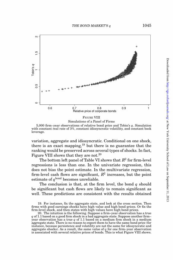
THE BOND MARKET’S q 1045
11.5
2T
ob
in's
q0
0.5
0.6 0.7 0.8 0.9 1Relative price of corporate bonds
FIGURE VIIISimulations of a Panel of Firms
5,000 firm–year observations of relative bond price and Tobin’s q. Simulationwith constant real rate of 3%, constant idiosyncratic volatility, and constant bookleverage.
variation, aggregate and idiosyncratic. Conditional on one shock,there is an exact mapping,19 but there is no guarantee that theranking would be preserved across several types of shocks. In fact,Figure VIII shows that they are not.20
The bottom left panel of Table VI shows that R2 for firm-levelregressions is less than one. In the univariate regression, thisdoes not bias the point estimate. In the multivariate regression,firm-level cash flows are significant, R2 increases, but the pointestimate of qbond becomes unreliable.
The conclusion is that, at the firm level, the bond q shouldbe significant but cash flows are likely to remain significant aswell. These predictions are consistent with the results obtained
19. For instance, fix the aggregate state, and look at the cross section. Thenfirms with good earnings shocks have high value and high bond prices. Or fix thefirm-level shock, and then states with high values have high bond prices.
20. The intuition is the following. Suppose a firm–year observation has a trueq of 1.1 based on a good firm shock in a bad aggregate state. Suppose another firm–year observation has a true q of 1.1 based on a medium firm shock in a mediumaggregate state. There is no reason to expect them to have the same bond price (forinstance, because persistence and volatility are not the same for idiosyncratic andaggregate shocks). As a result, the same value of q for one firm–year observationis associated with several relative prices of bonds. This is what Figure VIII shows.
at New
York U
niversity School of Law
on September 11, 2013
http://qje.oxfordjournals.org/D
ownloaded from
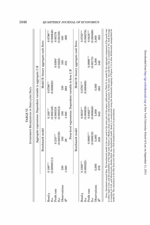
1046 QUARTERLY JOURNAL OF ECONOMICS
TA
BL
EV
II N
VE
ST
ME
NT
RE
GR
ES
SIO
NS
INS
IMU
LA
TE
DD
AT
A
Agg
rega
tere
gres
sion
s:D
epen
den
tva
riab
leis
aggr
egat
eI/
K
Ben
chm
ark
mod
elM
odel
B:b
inar
yag
greg
ate
cash
flow
s
Bon
dq
0.10
0∗∗∗
0.10
0∗∗∗
0.07
99∗∗
∗0.
0796
∗∗∗
S.e.
(0.0
0000
111)
(0.0
0014
8)(0
.000
623)
(0.0
0064
8)P
rofi
tra
te0.
210∗
∗∗−0
.000
318
0.03
94∗
0.00
176
S.e.
(0.0
0015
9)(0
.000
312)
(0.0
222)
(0.0
0158
)O
bser
vati
ons
100
100
100
100
100
100
R2
1.00
0.9
81.
000
.994
.031
.995
Fir
m-l
evel
regr
essi
ons:
Dep
ende
nt
vari
able
isfi
rmI/
K
Ben
chm
ark
mod
elM
odel
B:b
inar
yag
greg
ate
cash
flow
s
Bon
dq
0.10
00∗∗
∗0.
0610
∗∗∗
0.07
91∗∗
∗0.
0703
∗∗∗
S.e.
(0.0
0052
5)(0
.000
638)
(0.0
0040
8)(0
.000
276)
Pro
fit
rate
0.09
93∗∗
∗0.
0482
∗∗∗
0.08
98∗∗
∗0.
0434
∗∗∗
S.e.
(0.0
0061
9)(0
.000
649)
(0.0
0173
)(0
.000
498)
Obs
erva
tion
s5,
000
5,00
05,
000
5,00
05,
000
5,00
0R
2.8
79.8
38.9
43.8
83.3
49.9
53
Not
es.S
imu
late
dan
nu
alda
ta.T
he
ben
chm
ark
mod
elis
the
one
use
din
the
mai
npa
rtof
the
pape
r,ca
libr
ated
inT
able
II.I
nm
odel
B,t
he
aggr
egat
eco
mpo
nen
tof
the
profi
tra
teis
eith
erh
igh
orlo
w,a
nd
the
prob
abil
ity
ofth
eh
igh
stat
efo
llow
sa
Mar
kov
chai
nu
nde
rth
eri
sk-n
eutr
alm
easu
re.I
nbo
thca
ses,
the
risk
-fre
era
teis
con
stan
tat
3%,b
ook
leve
rage
isco
nst
ant
at0.
45,
and
idio
syn
crat
icsh
ocks
foll
owth
ebe
nch
mar
km
odel
.B
ond
qis
con
stru
cted
usi
ng
the
ben
chm
ark
map
pin
gof
Fig
ure
I(i
tis
thu
sde
libe
rate
lym
issp
ecifi
edfo
rm
odel
B).
Th
esi
mu
lati
onis
for
fift
yfi
rms
and
100
year
s.O
LS
stan
dard
erro
rsar
ein
pare
nth
eses
.
at New
York U
niversity School of Law
on September 11, 2013
http://qje.oxfordjournals.org/D
ownloaded from
THE BOND MARKET’S q 1047
by Gilchrist and Zakrajsek (2007) with a large panel data setof firm-level bond prices. They regress the investment rate on afirm-specific measure of the cost of capital, based on firm-levelbond yields and industry-specific prices for capital. They find astrong negative relationship between the investment rate and thecorporate yields, and they also find that qusual and cash flowsremain significant.
There are other explanations for the discrepancy between mi-cro and macro results. Returns to scale might be decreasing at thelevel of an individual firm, even though they are constant for theeconomy as a whole. This could explain why cash flows are signif-icant in the micro data but not in the macro data. Finally, to theextent that mispricing explains some of the discrepancy betweenqusual and qbond, the results are consistent with the argument inLamont and Stein (2006) that there is more mispricing at theaggregate level than at the firm level.
VII.B. Robustness to Model Misspecifications
I now turn to the issue of the specification of aggregate dynam-ics. The mapping in Figure I assumes that aggregate dynamics fol-low an AR(1) process. This is a restrictive assumption, especiallyunder the risk-neutral measure.21 A second model is thereforeused to check the robustness of the results. Model B (described inthe Appendix) is meant to be the polar opposite to the benchmarkmodel as far as aggregate dynamics are concerned (idiosyncraticshocks are unchanged). This model captures two important ideas.First, cash flows might have a short- and a long-run component,the long-run one being more relevant for valuation and invest-ment. Second, holding constant the objective distribution of cashflows, changes in the market price of risk (due to changes in riskaversion or conditional volatilities) affect the risk-neutral likeli-hood of good and bad states. In both cases, aggregate cash flowswould not summarize the aggregate state. This model is empir-ically relevant because Vuolteenaho (2002) shows that much ofthe volatility at the firm level reflects cash-flow news, whereasdiscount rate shocks are much more important in the aggregate.
I simulate a panel similar to the one discussed above (fiftyyears, 100 firms). I then use the mapping of Figure I to construct
21. Moreover, this assumption implies that the current aggregate profit rateis a sufficient statistic for the current aggregate state, which is clearly unrealistic.This can be seen in the simulated aggregate regressions where aggregate cashflows have an R2 of .98 (Table VI, column (2)).
at New
York U
niversity School of Law
on September 11, 2013
http://qje.oxfordjournals.org/D
ownloaded from
1048 QUARTERLY JOURNAL OF ECONOMICS
q. The model is therefore misspecified because the benchmarkmapping is used to construct qbond in a world where aggregatedynamics are substantially different from the benchmark.
The first result in Table VI is that the model retains most ofits explanatory power. qbond is a reliable predictor even when themodel is misspecified. The R2 is still close to one, at 99.4%. Theonly issue is the bias in the estimated coefficient, which overesti-mates adjustment costs by about 20%.
The second important message of Table VI is that cash flowsare not reliable in the aggregate regression. In model B, cashflows have no explanatory power for aggregate investment. Atthe firm level, cash flows remain significant, as expected, becausefirm-level dynamics is the same as in the benchmark model.
VII.C. Bankruptcy Costs and Leverage
The benchmark model is built under the assumptions of notaxes and no bankruptcy costs (Modigliani and Miller 1958).22 Inow study how qbond performs if there are taxes and bankruptcycosts. To focus on the crucial issues and to avoid heavy notations,I consider here a simple one-period example. Investment takesplace at the beginning of the period, and returns are realized atthe end. The risk-free rate is normalized to zero. Profits are taxedat a flat rate, payments to bondholders are deductible, and thereare bankruptcy costs. The details of the model are described inthe Appendix.
Figure IX shows the mappings for different values of distresscosts (in the range of values consistent with empirical estimates).Distress costs do not appear to invalidate the approach taken inthis paper. The shape of the mapping is similar across the variousmodels.23 If anything, higher bankruptcy costs make the mappingfrom relative bond prices to q more linear, and thus easier toestimate empirically.
VIII. CONCLUSION
This paper has shown that it is possible to construct Tobin’sq using bond prices, by bringing the insights of Black and Scholes
22. In such a world, capital structure is irrelevant, and arbitrary changes inleverage are possible without affecting investment. This issue was discussed atthe end of Section IV.
23. The fact that one mapping is higher than another on average is irrelevantbecause it relates only to the average value of q.
at New
York U
niversity School of Law
on September 11, 2013
http://qje.oxfordjournals.org/D
ownloaded from
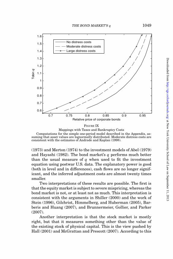
THE BOND MARKET’S q 1049
1
1.1
1.2
1.3
1.4
1.5
1.6T
obin
q
No distress costs
Moderate distress costs
Large distress costs
0.7 0.75 0.8 0.85 0.9 0.95
0.6
0.7
0.8
0.9
Relative price of corporate bonds
FIGURE IXMappings with Taxes and Bankruptcy Costs
Computations for the simple one-period model described in the Appendix, as-suming that asset values are lognormally distributed. Moderate distress costs areconsistent with the estimates of Andrade and Kaplan (1998).
(1973) and Merton (1974) to the investment models of Abel (1979)and Hayashi (1982). The bond market’s q performs much betterthan the usual measure of q when used to fit the investmentequation using postwar U.S. data. The explanatory power is good(both in level and in differences), cash flows are no longer signif-icant, and the inferred adjustment costs are almost twenty timessmaller.
Two interpretations of these results are possible. The first isthat the equity market is subject to severe mispricing, whereas thebond market is not, or at least not as much. This interpretation isconsistent with the arguments in Shiller (2000) and the work ofStein (1996), Gilchrist, Himmelberg, and Huberman (2005), Bar-beris and Huang (2007), and Brunnermeier, Gollier, and Parker(2007).
Another interpretation is that the stock market is mostlyright, but that it measures something other than the value ofthe existing stock of physical capital. This is the view pushed byHall (2001) and McGrattan and Prescott (2007). According to this
at New
York U
niversity School of Law
on September 11, 2013
http://qje.oxfordjournals.org/D
ownloaded from
1050 QUARTERLY JOURNAL OF ECONOMICS
view, firms accumulate and decumulate large stocks of intangiblecapital. If the payoffs from intangible capital were highly skewed,then they could affect equity prices more than bond prices, andthis could explain the results presented in this paper. The diffi-culty of this theory, of course, is that it rests on a stock of intangiblecapital that we cannot readily measure (see Atkeson and Kehoe[2005] for a plant-level analysis).
Looking back at Figure IV, it is difficult to imagine a satisfac-tory answer that does not mix the two theories. Moreover, thesetheories are not as contradictory as they appear, because the factthat intangible capital is hard to measure increases the scope fordisagreement and mispricing. One can hope that future researchwill be able to reconcile the two explanations.
APPENDIX
A. Proof of Proposition 1
Let θτ be the marginal default rate during period τ . Let �t,τ
be the cumulative default rate in periods t + 1 up to τ − 1. Inother words, if a bond has not defaulted at time t, the probabilitythat it enters time τ > t is 1 − �t,τ . Thus, by definition, �t,t+1 = 0and the default rates satisfy the recursive structure: 1 − �t,τ =(1 − θt+1)
(1 − �t+1,τ
). The value at the end of period t of one unit
of outstanding principal is
b1t = Eπ
t
[ ∞∑τ=t+1
(1 − �t,τ )(1 − φ)τ−t−1
(1 + rt,τ )τ−t((1 − θτ )(c + φ)
+ θτ Vτ /τ−1)].(22)
Similarly, and just to be clear, the price of one unit of principal atthe end of t + 1 is
b1t+1 = Eπ
t+1
[ ∞∑τ=t+2
(1 − �t+1,τ )(1 − φ)τ−t−2
(1 + rt+1,τ )τ−t−1((1 − θτ )(c + φ)
+ θτ Vτ /τ−1)].(23)
at New
York U
niversity School of Law
on September 11, 2013
http://qje.oxfordjournals.org/D
ownloaded from
THE BOND MARKET’S q 1051
Using the recursive structure of � and the law of iterated expec-tations, we can substitute (23) into (22) and obtain
b1t = 1
1 + rtEπ
t [(1 − θt+1)(c + φ) + θt+1Vt+1/t]
+ 1 − φ
1 + rtEπ
t
[(1 − θt+1)b1
t+1
].(24)
Default happens when equity value reaches zero, that is, when
Vt < t−1(φ + c + (1 − φ)b1
t
).
Therefore, the pricing function satisfies
b1t = 1
1 + rtEπ
t
[min
{φ + c + (1 − φ)b1
t+1; Vt+1/t}]
.(25)
Now recall that b1t is the price of one unit of outstanding capital.
Let us define bt as the value of bonds outstanding at the end oftime t, scaled by end-of-period physical assets,
bt ≡ ψb1t ,(26)
where book leverage was defined in the main text as ψ ≡ t/kt,and assumed to be constant. Multiplying both sides of (25) by ψ ,we obtain
bt = 11 + rt
Eπt [min{(φ + c)ψ + (1 − φ)bt+1; vt+1}].
In recursive form, and with constant book leverage, this leads toequation (7).
Note that if book leverage were state-contingent, the firstterm in the min function would simply be (φ + c)ψt + (1 − φ)bt+1ψt
ψt+1.
B. Proof of Proposition 3
Assume that GH > . We can then write the debt pricingformula (21) as
Bt = 11 + r
{(1 − λt)Eπ
t
[min
(t; vt+1kt + GL)] + λtt
}.(27)
at New
York U
niversity School of Law
on September 11, 2013
http://qje.oxfordjournals.org/D
ownloaded from
1052 QUARTERLY JOURNAL OF ECONOMICS
Taking the limit in equation (27) as λt → 0 and GL → 0, it is clearthat
Bt = 11 + r
Eπt [min(t; vt+1kt)].
This is the same pricing formula we used earlier, and we havealready seen that one can construct a sufficient statistic for in-vestment in this case. On the other hand, the market value of eq-uity moves when it is revealed that Gt = GH . It is always possibleto increase the variance of the shocks by increasing GH . Becausethese shocks are uncorrelated with investment, the explanatorypower of the traditional measure can become arbitrarily small.
Note that in a growing economy, it would make sense to indexthe growth option on aggregate TFP to obtain a model with abalanced growth path.
C. Model B
In this model, the conditional distribution of cash flows fol-lows a Markov process. Aggregate cash flows can be either high,aH , or low, aL, and the risk-neutral probability of observing a highcash flow is state-dependent:
Pr(a = aH) = f (s).
State s follows a four-state Markov process under the risk-neutralmeasure. The complete aggregate state is (s, a). There are there-fore eight possible aggregate states: four states for s and two for a.The persistence in the aggregate time series comes from the per-sistence in s. Conditional on s, aggregate cash flows are i.i.d. Thetransition matrix of s is chosen to match the empirical momentsin Table II. Firm-level dynamics η are given by equation (17) asin the benchmark model.
D. Distress Costs
This is a one-period model. Without taxes or bankruptcy costs,the program of the firm is
maxk
Eπ [vk] − k − γ k2/2,(28)
where k is investment and v is a random variable. Optimal invest-ment is
k = (q − 1)/γ,(29)
at New
York U
niversity School of Law
on September 11, 2013
http://qje.oxfordjournals.org/D
ownloaded from
THE BOND MARKET’S q 1053
where q ≡ Eπ [v]. Now assume that profits are taxed at rate τ ,that payments to bondholders are deductible, and that there areproportional bankruptcy costs ϕ. In case of default, a value ϕvk islost. The firm is financed with debt and equity, and let ψ be bookleverage. It is then straightforward to see that (29) still holds, butthe definition of q must be adjusted to
q ≡ (1 − τ )Eπ [v] + τ Eπ [min(ψ, v)] − ϕEπ [v1v<ψ ].(30)
The first term is the unlevered q. The second term captures thetax benefits of debt. The last term captures bankruptcy costs. Thevalue of debt (relative to book assets) is
b = Eπ [min(ψ, v)] − ϕEπ [v1v<ψ ].(31)
Equity is e = E[(1 − τ )(v − ψ)1v>ψ ]. Finally, optimal leveragesolves the program
maxψ
τ
∫ ∞
0min(ψ, v) dH(v) − ϕ
∫ ψ
0vdH(v),(32)
where H(.) is the cumulative distribution of v, and h(.) the asso-ciated density. The first term measures the tax benefits of debt,whereas the second term measures the deadweight losses fromfinancial distress. The first-order condition for optimal leverage is
τ
∫ ∞
ψ
dH(v) = ϕψh(ψ).(33)
I assume that v is lognormally distributed with volatility 0.75.In the benchmark case, I use ϕ = 0.2 and a lognormal mean of−0.2. These parameters yield values consistent with the evidencein Andrade and Kaplan (1998) and Almeida and Philippon (2007).Andrade and Kaplan (1998) estimate losses around 10%–15% offirm value one-year before bankruptcy. The parameter ϕ appliesto ex post losses, and these happen when v turns out to be low. Avalue of 20% implies that the deadweight losses relative to initialfirm value are around 10%. To be consistent with a book leverageof 0.5, equation (33) implies that τ = 11.5%. This is consistentwith Graham (2000).
The benchmark case is therefore chosen so that leverage isoptimal (on average, not state by state) and distress costs areconsistent with empirical estimates. To create Figure IX, I simu-late the model with different values of the mean of the lognormal
at New
York U
niversity School of Law
on September 11, 2013
http://qje.oxfordjournals.org/D
ownloaded from
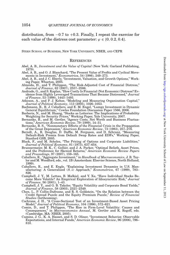
1054 QUARTERLY JOURNAL OF ECONOMICS
distribution, from −0.7 to +0.3. Finally, I repeat the exercise foreach value of the distress cost parameter: ϕ ∈ {0, 0.2, 0.4}.
STERN SCHOOL OF BUSINESS, NEW YORK UNIVERSITY, NBER, AND CEPR
REFERENCES
Abel, A. B., Investment and the Value of Capital (New York: Garland Publishing,1979).
Abel, A. B., and O. J. Blanchard, “The Present Value of Profits and Cyclical Move-ments in Investment,” Econometrica, 54 (1986), 249–273.
Abel, A. B., and J. C. Eberly, “Investment, Valuation, and Growth Options,” Work-ing Paper, Wharton, 2005.
Almeida, H., and T. Philippon, “The Risk-Adjusted Cost of Financial Distress,”Journal of Finance, 62 (2007), 2557–2586.
Andrade, G., and S. Kaplan, “How Costly Is Financial (Not Economic) Distress? Ev-idence from Highly Leveraged Transactions That Became Distressed,” Journalof Finance, 53 (1998), 1443–1493.
Atkeson, A., and P. J. Kehoe, “Modeling and Measuring Organization Capital,”Journal of Political Economy, 113 (2005), 1026–1053.
Bachmann, R., R. J. Caballero, and E. M. Engel, “Lumpy Investment in DynamicGeneral Equilibrium,” Cowles Foundation Discussion Paper 1566, 2006.
Barberis, N., and M. Huang, “Stocks as Lotteries: The Implications of ProbabilityWeighting for Security Prices,” Working Paper, Yale University, 2007.
Bernanke, B., and M. Gertler, “Agency Costs, Net Worth and Business Fluctua-tions,” American Economic Review, 79 (1989), 14–31.
Bernanke, B. S., “Nonmonetary Effects of the Financial Crisis in the Propagationof the Great Depression,” American Economic Review, 73 (1983), 257–276.
Berndt, A., R. Douglas, D. Duffie, M. Ferguson, and D. Schranz, “MeasuringDefault-Risk Premia from Default Swap Rates and EDFs,” Working Paper,Stanford GSB, 2005.
Black, F., and M. Scholes, “The Pricing of Options and Corporate Liabilities,”Journal of Political Economy, 81 (1973), 637–654.
Brunnermeier, M. K., C. Gollier, and J. A. Parker, “Optimal Beliefs, Asset Prices,and the Preference for Skewed Returns,” American Economic Review Papersand Proceedings, 97 (2007), 159–165.
Caballero, R., “Aggregate Investment,” in Handbook of Macroeconomics, J. B. Tay-lor and M. Woodford, eds., vol. 1B (Amsterdam: Elsevier Science, North Holland,1999).
Caballero, R., and E. Engle, “Explaining Investment Dynamics in U.S. Man-ufacturing: A Generalized (S, s) Approach,” Econometrica, 67 (1999), 783–826.
Campbell, J. Y., M. Lettau, B. Malkiel, and Y. Xu, “Have Individual Stocks Be-come More Volatile? An Empirical Exploration of Idiosyncratic Risk,” Journalof Finance, 56 (2001), 1–43.
Campbell, J. Y., and G. B. Taksler, “Equity Volatility and Corporate Bond Yields,”Journal of Finance, 58 (2003), 2321–2349.
Chen, L., P. Collin-Dufresne, and R. S. Goldstein, “On the Relation between theCredit Spread Puzzle and the Equity Premium Puzzle,” Review of FinancialStudies (forthcoming).
Cochrane, J. H., “A Cross-Sectional Test of an Investment-Based Asset PricingModel,” Journal of Political Economy, 104 (1996), 572–621.
Comin, D., and T. Philippon, “The Rise in Firm-Level Volatility: Causes andConsequences,” in Macroeconomics Annual, M. Gertler and K. Rogoff, eds.(Cambridge, MA: NBER, 2005).
Cumins, J. G., K. A. Hasset, and S. D. Oliner, “Investment Behavior, ObservableExpectations, and Internal Funds,” American Economic Review, 96 (2006), 796–810.
at New
York U
niversity School of Law
on September 11, 2013
http://qje.oxfordjournals.org/D
ownloaded from
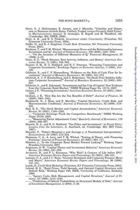
THE BOND MARKET’S q 1055
Davis, S., J. Haltiwanger, R. Jarmin, and J. Miranda, “Volatility and Disper-sion in Business Growth Rates: Publicly Traded versus Privately Held Firms,”in Macroeconomics Annual, D. Acemoglu, K. Rogoff, and M. Woodford, eds.(Cambridge, MA: NBER, 2006).
Dixit, A. K., and R. S. Pindyck, Investment under Uncertainty (Princeton, NJ:Princeton University Press, 1994).
Duffie, D., and K. J. Singleton, Credit Risk (Princeton, NJ: Princeton UniversityPress, 2003).
Erickson, T., and T. M. Whited, “Measurement Error and the Relationship betweenInvestment and Q,” Journal of Political Economy, 108 (2000), 1027–1057.
——, “On the Accuracy of Different Measures of Q,” Financial Management, 35(2006), 5–33.
Fama, E. F., “Stock Returns, Real Activity, Inflation, and Money,” American Eco-nomic Review, 71 (1981), 545–565.
Fazzari, S. M., R. G. Hubbard, and B. C. Petersen, “Financing Constraints andCorporate Investment,” Brookings Papers on Economic Activity, 1 (1988), 141–195.
Gilchrist, S., and C. P. Himmelberg, “Evidence on the Role of Cash Flow for In-vestment,” Journal of Monetary Economics, 36 (1995), 541–572.
Gilchrist, S., C. P. Himmelberg, and G. Huberman, “Do Stock Price Bubbles Influ-ence Corporate Investment?” Journal of Monetary Economics, 52 (2005), 805–827.
Gilchrist, S., and E. Zakrajsek, “Investment and the Cost of Capital: New Evidencefrom the Corporate Bond Market,” NBER Working Paper No. 13174, 2007.
Gomes, J. F., “Financing Investment,” American Economic Review, 91 (2001), 1263–1285.
Graham, J. R., “How Big Are the Tax Benefits of Debt?” Journal of Finance, 55(2000), 1901–1941.
Hackbarth, D., J. Miao, and E. Morellec, “Capital Structure, Credit Risk, andMacroeconomic Conditions,” Journal of Financial Economics, 82 (2006), 519–550.
Hall, R. E., “The Stock Market and Capital Accumulation,” American EconomicReview, 91 (2001), 1185–1202.
——, “Corporate Earnings Track the Competitive Benchmark,” NBER WorkingPaper 10150, 2003.
——, “Measuring Factor Adjustment Costs,” Quarterly Journal of Economics, 119(2004), 899–927.
Hassett, K. A., and R. G. Hubbard, “Tax Policy and Investment,” in Fiscal Policy:Lessons from the Literature, A. Auerbach, ed. (Cambridge, MA: MIT Press,1997).
Hayashi, F., “Tobin’s Marginal q and Average q: A Neoclassical Interpretation,”Econometrica, 50 (1982), 213–224.
Hennessy, C. A., A. Levy, and T. M. Whited, “Testing Q Theory with FinancingFrictions,” Journal of Financial Economics, 83 (2007), 691–717.
Hilscher, J., “Is the Corporate Bond Market Foward Looking?” Working Paper,Brandeis University, 2007.
Jorgenson, D. W., “Capital Theory and Investment Behavior,” American EconomicReview, 53 (1963), 247–259.
Jovanovic, B., and P. L. Rousseau, “Why Wait? A Century of Life before IPO,”American Economic Review Papers and Proceedings, 91 (2001), 336–341.
Lamont, O. A., and J. C. Stein, “Investor Sentiment and Corporate Finance: Microand Macro,” American Economic Review Papers and Proceedings, 96 (2006),147–151.
Lando, D., Credit Risk Modeling (Princeton, NJ: Princeton University Press, 2004).Leland, H. E., “Bond Prices, Yield Spreads, and Optimal Capital Structure with
Default Risk,” Working Paper 240, IBER, University of California, Berkeley,1994.
——, “Agency Costs, Risk Management, and Capital Structure,” Journal of Fi-nance, 53 (1998), 1213–1243.
——, “Predictions of Default Probabilities in Structural Models of Debt,” Journalof Investment Management, 2 (2004), 5–20.
at New
York U
niversity School of Law
on September 11, 2013
http://qje.oxfordjournals.org/D
ownloaded from
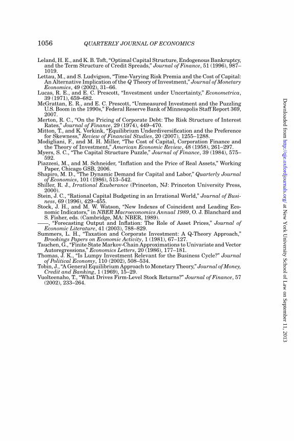
1056 QUARTERLY JOURNAL OF ECONOMICS
Leland, H. E., and K. B. Toft, “Optimal Capital Structure, Endogenous Bankruptcy,and the Term Structure of Credit Spreads,” Journal of Finance, 51 (1996), 987–1019.
Lettau, M., and S. Ludvigson, “Time-Varying Risk Premia and the Cost of Capital:An Alternative Implication of the Q Theory of Investment,” Journal of MonetaryEconomics, 49 (2002), 31–66.
Lucas, R. E., and E. C. Prescott, “Investment under Uncertainty,” Econometrica,39 (1971), 659–682.
McGrattan, E. R., and E. C. Prescott, “Unmeasured Investment and the PuzzlingU.S. Boom in the 1990s,” Federal Reserve Bank of Minneapolis Staff Report 369,2007.
Merton, R. C., “On the Pricing of Corporate Debt: The Risk Structure of InterestRates,” Journal of Finance, 29 (1974), 449–470.
Mitton, T., and K. Vorkink, “Equilibrium Underdiversification and the Preferencefor Skewness,” Review of Financial Studies, 20 (2007), 1255–1288.
Modigliani, F., and M. H. Miller, “The Cost of Capital, Corporation Finance andthe Theory of Investment,” American Economic Review, 48 (1958), 261–297.
Myers, S. C., “The Capital Structure Puzzle,” Journal of Finance, 39 (1984), 575–592.
Piazzesi, M., and M. Schneider, “Inflation and the Price of Real Assets,” WorkingPaper, Chicago GSB, 2006.
Shapiro, M. D., “The Dynamic Demand for Capital and Labor,” Quarterly Journalof Economics, 101 (1986), 513–542.
Shiller, R. J., Irrational Exuberance (Princeton, NJ: Princeton University Press,2000).
Stein, J. C., “Rational Capital Budgeting in an Irrational World,” Journal of Busi-ness, 69 (1996), 429–455.
Stock, J. H., and M. W. Watson, “New Indexes of Coincident and Leading Eco-nomic Indicators,” in NBER Macroeconomics Annual 1989, O. J. Blanchard andS. Fisher, eds. (Cambridge, MA: NBER, 1989).
——, “Forecasting Output and Inflation: The Role of Asset Prices,” Journal ofEconomic Literature, 41 (2003), 788–829.
Summers, L. H., “Taxation and Corporate Investment: A Q-Theory Approach,”Brookings Papers on Economic Activity, 1 (1981), 67–127.
Tauchen, G., “Finite State Markov-Chain Approximations to Univariate and VectorAutoregressions,” Economics Letters, 20 (1986), 177–181.
Thomas, J. K., “Is Lumpy Investment Relevant for the Business Cycle?” Journalof Political Economy, 110 (2002), 508–534.
Tobin, J., “A General Equilibrium Approach to Monetary Theory,” Journal of Money,Credit and Banking, 1 (1969), 15–29.
Vuolteenaho, T., “What Drives Firm-Level Stock Returns?” Journal of Finance, 57(2002), 233–264.
at New
York U
niversity School of Law
on September 11, 2013
http://qje.oxfordjournals.org/D
ownloaded from