University of Melbourne

School of Mathematics and Statistics

The Blockchain Propagation Process: a Machine

Learning and Matrix Analytic Approach

Aapeli Vuorinen

supervised byProfessor Peter Taylor

A thesis submitted for the degree of

Master of Science

May 17, 2019

Abstract

Blockchain, spearheaded by the Bitcoin cryptocurrency, is a novel, emerging technology that allows adistributed network of users to synchronise and maintain a decentralised, global ledger of transactionswith no central control or authority. One key part of this technology is the process by which blocks andtransactions propagate through the underlying network of users, allowing them to come to a consensuson the state of the ledger and advance the blockchain. In this thesis, we explored the propagationprocess for Bitcoin within the mathematical framework of matrix analytic processes by performing anobservational experiment to collect data and fitting phase-type distributions to this dataset.

It is well known that the propagation delay of blocks is a key limiting factor in the efficiency andscalability of blockchain technology. It is imperative that the network reaches an overall consensuson the current state of the chain of blocks at regular epochs. If blocks propagate faster through thenetwork, then this happens faster and the time between blocks can be decreased. This means thatthe blockchain can then process more events as well as verify those events faster. Additionally, recentwork on a strategy known as selfish-mining has shown that adversarial miners can take advantage ofthis delay to inflate their share of mining rewards.

We set out to model the block propagation process of Bitcoin blocks. To do so, we set up a dis-tributed, large-scale observational experiment by creating a global data collection system for observingthe block propagation process. We collected data on the propagation patterns of 14810 blocks over 5months from November 2018 until March 2019, and created a novel tool for observing the blockchainfrom several geographically diverse locations.

We fitted Coxian phase-type distributions of a varying number of phases to the data and performedmodel selection, finally choosing a model with p = 4 phases. We used a variant of the EM-algorithmoriginally introduced by Asmussen, and made improvements to the computational run-time of thealgorithm. We present the final parameter estimates of our model and discuss the merits and short-comings of this approach.

This thesis makes three contributions. The first is an open dataset of Bitcoin block propagationdata which we have cleaned and pre-processed to include additional covariates extracted from theblockchain. We present a short exploratory data analysis of patterns in the dataset in Part III. Oursecond contribution is a phase-type model for the block propagation delay, which we discuss in PartII. Finally, we have made an incremental improvement to the EM-algorithm for fitting phase-typedistributions by parallelising it and reducing its memory footprint, which is particularly useful forvery large, “big data” datasets. We also believe that our exposition describing the Bitcoin ecosystemin Part I is of value.

We have created an accompanying website at https://bitcoin.aapelivuorinen.com/, whichcontains complementary material, the cleaned dataset, the source code for data collection, and ourimproved phase-type fitting algorithm.

1

Acknowledgments

I wish to express my gratitude towards Peter Taylor for his patient, inspiring supervision, and forproviding me with direction when I needed it through insightful comments and criticism.

I would like to thank my good friend and mentor, Yoni Nazarathy for his continuous encouragement,support, and guidance over the past years, both in mathematics and in life.

Finally, I would like to thank the friends and family who supported me through this endeavour.

2

Contents

Abstract 1

Acknowledgments 2

1 Introduction 51.1 Outline of the thesis . . . . . . . . . . . . . . . . . . . . . . . . . . . . . . . . . . . . . . . . . . . . . . . 7

I Bitcoin 8

2 Overview of the Bitcoin ecosystem 92.1 Overview of cryptographic primitives . . . . . . . . . . . . . . . . . . . . . . . . . . . . . . . . . . . . . . 10

2.1.1 Digital signatures . . . . . . . . . . . . . . . . . . . . . . . . . . . . . . . . . . . . . . . . . . . . . 102.1.2 Cryptographically hash functions . . . . . . . . . . . . . . . . . . . . . . . . . . . . . . . . . . . . 102.1.3 Proof-of-work schemes . . . . . . . . . . . . . . . . . . . . . . . . . . . . . . . . . . . . . . . . . . 112.1.4 Merkle trees . . . . . . . . . . . . . . . . . . . . . . . . . . . . . . . . . . . . . . . . . . . . . . . . 12

2.2 The structure of the blockchain . . . . . . . . . . . . . . . . . . . . . . . . . . . . . . . . . . . . . . . . . 122.2.1 Addresses and wallets . . . . . . . . . . . . . . . . . . . . . . . . . . . . . . . . . . . . . . . . . . 122.2.2 Transactions . . . . . . . . . . . . . . . . . . . . . . . . . . . . . . . . . . . . . . . . . . . . . . . 132.2.3 Blocks and the mining process . . . . . . . . . . . . . . . . . . . . . . . . . . . . . . . . . . . . . 132.2.4 51 % attacks and double spending . . . . . . . . . . . . . . . . . . . . . . . . . . . . . . . . . . . 162.2.5 Application-Specific Integrated Circuits . . . . . . . . . . . . . . . . . . . . . . . . . . . . . . . . 172.2.6 Mining pools . . . . . . . . . . . . . . . . . . . . . . . . . . . . . . . . . . . . . . . . . . . . . . . 172.2.7 The block size limit and SegWit transactions . . . . . . . . . . . . . . . . . . . . . . . . . . . . . 18

2.3 The Bitcoin protocol . . . . . . . . . . . . . . . . . . . . . . . . . . . . . . . . . . . . . . . . . . . . . . . 182.3.1 Protocol messages . . . . . . . . . . . . . . . . . . . . . . . . . . . . . . . . . . . . . . . . . . . . 182.3.2 Nodes and peers . . . . . . . . . . . . . . . . . . . . . . . . . . . . . . . . . . . . . . . . . . . . . 182.3.3 Peer discovery . . . . . . . . . . . . . . . . . . . . . . . . . . . . . . . . . . . . . . . . . . . . . . 192.3.4 Control messages: version/verack, ping/pong, getaddr/addr . . . . . . . . . . . . . . . . . . . . 192.3.5 Data messages: inv, getdata, tx, block, getheaders/headers . . . . . . . . . . . . . . . . . . . . 192.3.6 The transaction propagation process . . . . . . . . . . . . . . . . . . . . . . . . . . . . . . . . . . 202.3.7 The block propagation process . . . . . . . . . . . . . . . . . . . . . . . . . . . . . . . . . . . . . 20

3 Data collection and the bitcoin-crawler 213.1 Overview . . . . . . . . . . . . . . . . . . . . . . . . . . . . . . . . . . . . . . . . . . . . . . . . . . . . . 213.2 The bitcoin-crawler . . . . . . . . . . . . . . . . . . . . . . . . . . . . . . . . . . . . . . . . . . . . . . 213.3 The global data collection system . . . . . . . . . . . . . . . . . . . . . . . . . . . . . . . . . . . . . . . . 233.4 Blockchain data and mining pools . . . . . . . . . . . . . . . . . . . . . . . . . . . . . . . . . . . . . . . 233.5 Cleaning of nonsensical data . . . . . . . . . . . . . . . . . . . . . . . . . . . . . . . . . . . . . . . . . . . 24

4 The dataset 254.1 Overview of the dataset . . . . . . . . . . . . . . . . . . . . . . . . . . . . . . . . . . . . . . . . . . . . . 254.2 Accompanying website and source code . . . . . . . . . . . . . . . . . . . . . . . . . . . . . . . . . . . . 27

II Mathematical modelling 28

5 Mathematical preliminaries 295.1 Continuous time Markov chains . . . . . . . . . . . . . . . . . . . . . . . . . . . . . . . . . . . . . . . . . 295.2 Phase-type distributions . . . . . . . . . . . . . . . . . . . . . . . . . . . . . . . . . . . . . . . . . . . . . 31

5.2.1 Examples of phase-type distributions . . . . . . . . . . . . . . . . . . . . . . . . . . . . . . . . . . 325.2.2 Coxian distributions . . . . . . . . . . . . . . . . . . . . . . . . . . . . . . . . . . . . . . . . . . . 33

5.3 The expectation-maximisation algorithm . . . . . . . . . . . . . . . . . . . . . . . . . . . . . . . . . . . . 335.4 Fitting phase-type distributions to data . . . . . . . . . . . . . . . . . . . . . . . . . . . . . . . . . . . . 355.5 Properties of the algorithm . . . . . . . . . . . . . . . . . . . . . . . . . . . . . . . . . . . . . . . . . . . 375.6 Akaike’s Information Criterion . . . . . . . . . . . . . . . . . . . . . . . . . . . . . . . . . . . . . . . . . 385.7 MapReduce . . . . . . . . . . . . . . . . . . . . . . . . . . . . . . . . . . . . . . . . . . . . . . . . . . . . 38

3

6 Computational aspects of phase-type fitting 396.1 The integral ΓΓΓ . . . . . . . . . . . . . . . . . . . . . . . . . . . . . . . . . . . . . . . . . . . . . . . . . . 39

6.1.1 The EMpht.c program . . . . . . . . . . . . . . . . . . . . . . . . . . . . . . . . . . . . . . . . . . 406.1.2 The EMpht.jl program . . . . . . . . . . . . . . . . . . . . . . . . . . . . . . . . . . . . . . . . . . 416.1.3 Uniformisation methods . . . . . . . . . . . . . . . . . . . . . . . . . . . . . . . . . . . . . . . . . 41

6.2 Our program . . . . . . . . . . . . . . . . . . . . . . . . . . . . . . . . . . . . . . . . . . . . . . . . . . . 436.3 Computation of the conditional expectations . . . . . . . . . . . . . . . . . . . . . . . . . . . . . . . . . 43

7 Phase-type fits to propagation delays 447.1 Method . . . . . . . . . . . . . . . . . . . . . . . . . . . . . . . . . . . . . . . . . . . . . . . . . . . . . . 457.2 Model selection . . . . . . . . . . . . . . . . . . . . . . . . . . . . . . . . . . . . . . . . . . . . . . . . . . 457.3 Discussion . . . . . . . . . . . . . . . . . . . . . . . . . . . . . . . . . . . . . . . . . . . . . . . . . . . . . 46

7.3.1 Basic statistics . . . . . . . . . . . . . . . . . . . . . . . . . . . . . . . . . . . . . . . . . . . . . . 477.3.2 Interval-censoring and censoring of the tail . . . . . . . . . . . . . . . . . . . . . . . . . . . . . . 487.3.3 Interpretation as propagation delay . . . . . . . . . . . . . . . . . . . . . . . . . . . . . . . . . . . 487.3.4 Further extensions . . . . . . . . . . . . . . . . . . . . . . . . . . . . . . . . . . . . . . . . . . . . 48

III Exploratory Data Analysis and Further Questions 50

8 Patterns in the dataset 518.1 Inter-arrival times of blocks . . . . . . . . . . . . . . . . . . . . . . . . . . . . . . . . . . . . . . . . . . . 518.2 Difference between timestamp in the block header and the arrival time . . . . . . . . . . . . . . . . . . . 528.3 Empty and full blocks, size and weight . . . . . . . . . . . . . . . . . . . . . . . . . . . . . . . . . . . . . 538.4 Block size and number of transactions . . . . . . . . . . . . . . . . . . . . . . . . . . . . . . . . . . . . . 558.5 Empty blocks and mining pools . . . . . . . . . . . . . . . . . . . . . . . . . . . . . . . . . . . . . . . . . 558.6 Causes of delay . . . . . . . . . . . . . . . . . . . . . . . . . . . . . . . . . . . . . . . . . . . . . . . . . . 568.7 Delay and location . . . . . . . . . . . . . . . . . . . . . . . . . . . . . . . . . . . . . . . . . . . . . . . . 58

Conclusion 62

IV Appendices 63

A Maximum likelihood estimators for transition rates and initialisation probabilities of a Markovchain 64

B Computation of conditional expectations 66

C Computations for the integral ΓΓΓ as the exponential of a block matrix 69

4

Chapter 1

Introduction

Bitcoin, conceived by Nakamoto in 2008 [1], is a decentralised electronic payment system that intro-

duced the concept of a blockchain. Often referred to as a cryptocurrency, Bitcoin relies on asymmetric

cryptography to manage addresses which act as containers for Bitcoins, and to authorise transactions

from one such address to another using digital signatures. These transactions are broadcasted onto

a public network where several entities operate as “miners”; working to bundle these transactions

together into blocks in exchange for a reward. Miners continuously work on solving a computation-

ally difficult problem, and each time a miner finds a solution to the problem, a new block is mined.

The difficulty of this computational problem, known as the proof-of-work, is regularly adjusted so

that blocks occur on average every ten minutes. Each block references the last block in the chain,

constructing a succession of blocks known as the blockchain.

Outside of the research community, Bitcoin has seen high uptake due to its innovative, decentralised

design which renders control by any entity impossible, and the ideals of distributed self-governance

in the absence of trust that it represents. However, its exchange rate has been a source of intense

speculation and coupled with its high volatility, slow transaction times, and high fees, the ability

of Bitcoin to act as a currency or stable store of value is limited. In addition, a lack of control by

regulatory authorities has led to a surge of Bitcoin’s use in illicit transactions, which in turn drives it

further away from legitimate industry.

Nonetheless, as it matures, blockchain technology continues to draw increased interest from the

technology sector, with several startups and established enterprises alike exploring blockchain tech-

nology as a solution to their business needs. Technical problems still exist with tying together the

boundary between real world events and the self-governing blockchain, as well as in scalability and ef-

ficiency. Several iterations of blockchains have been proposed and created since Bitcoin, implementing

new and exciting features such as smart contracts, allowing intricate custom logic to be implemented

on a blockchain.

Blockchain itself, an inventive human construct, has given rise to a multitude of interesting phe-

nomena, attracting researchers from many fields to study it from several perspectives and approaches.

Research on the emerging behaviour and properties of blockchain lies at the intersection of several

communities, including the applied probability and modelling community, the game theoretic com-

munity, the networking and topology inference community, as well as the distributed systems and

database community within computer science. These areas often overlap, giving rise to fruitful dis-

cussions between different communities and cultivating cross collaboration across fields of research. A

unique property of blockchain is that the full history of transactions and events that were accepted

into the ledger are readily available, which opens up further avenues for research.

5

From a probabilistic modelling perspective, the blockchain structure and the processes underlying

its construction present several interesting questions to be studied. This includes the block arrival

process which is modelled in [2], and double spending attacks as modelled in [3]. Other extensions

exploring the behaviour of systems similar to blockchain have been proposed, such as those where

the rate of blocks being produced is much higher than the rate at which the network can propagate

those nodes to every node to reach a consensus, leading to a random tree structure instead of one

resembling a chain with occasional branches.

The incentives underpinning the mining process, coupled with the rare yet considerable reward for

mining a block, make the process an interesting construct to study from the angle of game theory.

One interesting model for miner behaviour is the selfish-mine strategy introduced in [4], and further

studied by Gobel et al. under the presence of propagation delay in [5]; who show that miners can inflate

their share of mining rewards using this strategy. Others have studied the behaviour of mining pools,

groups of miners who band together share the burden and rewards in order to reduce the variance

in the revenue of their mining operations. In [6], the authors examine the dynamics of mining pools

the framework of cooperative game theory. The reward from mining blocks will eventually disappear,

presumably as miners should be rewarded from transaction fees. The implications of having blocks

without an intrinsic reward are studied in [7].

The control packets and the structure of the ad-hoc, peer-to-peer network underlying blockchains

are fundamentally different from those of other pre-existing networks such as the internet. This

provides an exciting challenge for the networking community in attempting to infer the topology of

the network. Much research has been done on revealing the topology of the underlying network using

both active and passive methods; for instance, a method exploiting the Bitcoin protocol was developed

in [8], in [9] inference was performed using a Bayesian approach, and in [10] a timing analysis based

method was developed. It is a rapidly evolving field, with the Bitcoin protocol being continuously

adjusted to counteract each new inference technique soon after it is published.

Finally, blockchain is studied by the distributed systems and databases community in computer

science, who are mainly interested in the scalability and efficiency of the system as a database and

distributed system. The work in this field ranges from modelling blockchain as a distributed system as

in [11], to proposing new consensus protocols to overcome the limitations of the current proof-of-work

solutions. Several authors have studied Byzantine fault-tolerance as an alternative, see [12] for an

overview of recent developments. Approaches to overcome scalability issues in blockchain currently

consist of two major branches: using sharding to distribute the blockchain across the network as

in [13], and using off-chain transaction networks to reduce the amount of data stored on the main

network. The Lightning network currently in development for Bitcoin is an example of the latter.

The aim of this work is to explore aspects of the block propagation process of Bitcoin, in particular,

the structure of delays, and the time taken for the network to reach consensus. To this end, we

performed a large-scale observational experiment and collected data on the propagation patterns of

14810 blocks between November 2018 and March 2019. We then fitted several phase-type models to

this data, discussing the fits and producing an estimate of the delay distribution. In the last part,

we have also made an effort to further explore the collected data and open up new research questions

that may be investigated using it, by performing an exploratory data analysis.

The contributions of this thesis are threefold. Firstly, we created both a tool and an open, high

quality dataset for studying the Bitcoin network. Secondly, we produced estimates and fits of the prop-

agation delay using phase-type distributions. Finally, we made a small improvement to the algorithm

for fitting phase-type distributions by increasing its performance for extremely large datasets.

6

1.1 Outline of the thesis

We begin in Part I by discussing the concepts underlying Bitcoin, and the system we developed to

observe the propagation process. Chapter 2 provides a thorough explanation of the Bitcoin ecosystem

and in Chapters 3 and 4 we explain our data collection and cleaning methodology, and give an overview

of the dataset. We hope that Part I is of value to a general audience.

In Part II we perform our mathematical modelling. In Chapter 5 we introduce the concept of

phase-type distributions and develop the theory of maximum likelihood parameter estimation for this

family of distributions using the EM-algorithm, while also discussing model selection using Akaike’s

information criterion and the MapReduce paradigm for data processing. Furthermore, in Chapter

6 we survey recent literature and new improvements on fitting phase-type distributions. Finally, in

Chapter 7 we present our phase-type fits and discuss the various ways of extending the model.

Part III consists of a further exploration of the dataset from a less rigorous perspective through

an exploratory data analysis. We present some interesting patterns we observed and discuss further

research questions that could be investigated from this data.

7

Part I

Bitcoin

8

Chapter 2

Overview of the Bitcoin ecosystem

Bitcoin is an electronic payment system introduced in 2008 in [1] and implemented several months

later in 2009 as the Bitcoin reference client [14]. It is interesting for its decentralised design which

allows it to operate without a central clearing house or a universally trusted authority. This is achieved

through a novel and technically creative incentive structure which ties together each entity taking part

in the Bitcoin community allowing it to follow a set of predefined rules while operating autonomously.

Bitcoin itself is comprised of two parts. The first consists of the blockchain data structure, a

distributed ledger of transactions, as well as the rules guiding its evolution dictating how the ledger

advances. These rules are known as the consensus rules. The second part is the network protocol

which allows users on the network to transmit this information between one another, and keep the

blockchain synchronised between users. Computers connected to the network are referred to as nodes,

and two computers connected to each other are called peers of each other. This thesis touches on both

aspects of Bitcoin, and in some sense, it can be seen as studying the intersection and interplay of the

two.

When a new block is mined or a new transaction is created, the information contained in it must

be transmitted by the underlying network protocol to all the nodes in the network. However, this

process is not instantaneous due to processing and network delays, which leads to a propagation delay:

the time between when a new object is introduced to the network and when it reaches a given node.

We call the time at which a new block is mined the block arrival time, or if talking about a particular

location, then the block arrival time refers to the time at which the block was first observed at that

location.

The propagation delay is extremely important. In the case of a newly mined block, an increased

delay leads to the network as a whole taking longer to reach consensus. Due to the nature of the

blockchain, it is not enough for a block to be mined for it to be immutably in the chain. As shown by

Nakamoto in the original Bitcoin paper [1], the probability of an adversary who wishes to overwrite

the blockchain succeeding drops off exponentially with the number of blocks that they are trying to

overwrite. One should therefore only consider a transaction or block permanently confirmed after it

is several blocks deep in the blockchain. This means that it takes several times the block inter-arrival

time for a transaction to be processed. This hinders the scalability and adoption of blockchain, as a

blockchain system with a long block inter-arrival time can include fewer transactions per unit time

and takes a longer time to process each transaction.

With an increased propagation delay, certain types of predictable delays may make topology infer-

ence tractable, allowing well-funded adversaries to correlate transactions with nodes on the network,

corroding the pseudonymity of Bitcoin users. In a sense, imperfections in the underlying network

9

protocol may leak information about the users of the Bitcoin ecosystem built on top of it.

This chapter is largely based on the source code of the Bitcoin reference client in [14], as well as

the author’s experience with blockchain and Bitcoin.

2.1 Overview of cryptographic primitives

This section gives an overview of the cryptographic primitives and ideas used in Bitcoin. The system

relies heavily on asymmetric cryptography through elliptic curve cryptography to sign and verify

transactions; and on cryptographically secure hash functions for its proof-of-work feature. The latter

is additionally used in a special structure called a Merkle tree, also discussed in this section.

2.1.1 Digital signatures

Elliptic curve cryptography is a central building block of Bitcoin. It allows users to securely and

independently sign a transaction when they wish to transfer Bitcoins, proving that they authorised it,

akin to the purpose of real-world signatures on cheques. These elliptic curve digital signatures exploit

properties of groups defined on elliptic curves over Galois fields to construct a scheme for digitally

signing a piece of binary data using asymmetric key pairs; that is, pairs of keys consisting of a private

and a public component. As we only give a high-level overview of the primitives, interested readers

are referred to [15] and [16] for a thorough introduction to elliptic curve cryptosystems and [17] for

details on the elliptic curve parameters used in Bitcoin.

An asymmetric cryptographic scheme consists of two routines, one for signing data and one for

verifying a signature. These routines require the use of an asymmetric key pair, consisting of a private

key to be safeguarded by the user, and the public key against which a signature is verified. The

private key consists of a randomly generated number, from which the public key is derived. The

signing routine can be seen as a function which takes as its inputs a private key and binary data to

be signed and outputs a digital signature. The verification routine on the other hand takes a digital

signature, binary data, and a public key and returns a binary value indicating whether the signature

matches the data and public key or not.

Asymmetric cryptosystems are generally constructed by way of a trapdoor function: a function

that is easy to compute given either the public key or the private key, and easy to invert given

the private key, but whose inverse is intractable unless one possesses also the private key. In the

case of elliptic curve cryptography, the underlying trapdoor function is the discrete logarithm on the

Galois field at hand [15]. Importantly, the security of these cryptosystems relies on it really being

difficult to compute the inverse of the trapdoor function without the private key, which relies on

the assumption that P 6= NP ; one of the major unsolved problems in theoretical computer science.

Furthermore, if P = NP , then this inverse can be computed in polynomial time, breaking most

asymmetric cryptosystems in use.

2.1.2 Cryptographically hash functions

Bitcoin uses cryptographically secure hashing extensively in its proof-of-work construct and the way it

refers to objects. A general hash function is any function that takes an arbitrary length binary string

and outputs a fixed size binary string. Hash functions are used in several areas of computer science

such hash tables and non-cryptographic checksums, where one generally hopes they are fast and that

values rarely map to the same output. Cryptographic hash functions1 are a subset of hash functions

1Again, the theoretical existence of such functions relies on P 6= NP .

10

that make them appropriate for use in cryptography by having the following additional properties:

1. the input is completely uncorrelated to the output, so even a small change in the input completely

scrambles the output;

2. given an arbitrary hash, it is computationally infeasible to find an input that matches this hash;

and

3. it is computationally infeasible to find two inputs with the same hash.

These functions are useful in the verification and attestation of information. For instance, suppose

we had a large blob of data that needed to be transferred from one location to another. Computing a

cryptographic hash of the content before and after the transfer would then provide us with a convenient

way of verifying that each bit was correct, meaning we only need to verify n bits for a hash of length

n instead of all the bits in the data. A common use of hashing is in signing full documents: digitally

signing long binary documents tends to be extremely slow if not impossible, so instead the document

is cryptographically hashed, and that short binary string is signed instead.

Most objects referred to in Bitcoin are identified by the hashes of their contents, a property known

as content-addressability. For instance, a transaction has a canonical encoding as a certain binary

string, and so instead of having some form of transaction number or other reference, transactions

are referred to by the hash of their canonical encoding. Similarly, a block has a canonical encoding,

and so each block is also referred to by its hash. This referencing method only works because it is

computationally infeasible to create a new transaction or block with the same hash. The hashing

algorithm used in Bitcoin for content-addressability is the double SHA-256 hash.

2.1.3 Proof-of-work schemes

The first property of cryptographic hash functions means that the output should be completely ran-

dom. That is, the output for any set of distinct inputs should be uniformly and independently

distributed over the possible outputs of that hash function (a binary string of fixed length n can be

identified with a non-negative integer between 0 and 2n − 1).

We can use this property to construct a “proof-of-work” scheme. Suppose we would like another

user to prove that they have performed a certain amount of work before accepting some data from

them; for instance to fight email spam. We may proceed as follows: the user first takes the hash of

their data and affixes to it a random binary string called a nonce. They then compute some predefined

cryptographic hash of this concatenated data, which is some integer between 0 and 2n − 1. If this

result is lower than some predefined difficulty threshold, then we accept the data. Otherwise, we

require that the user changes the nonce and repeats the computation until producing a valid hash.

By altering the difficulty threshold, we can adjust the expected number of computations that the user

must perform before producing acceptable data, hence probabalistically “proving” that they have

performed a certain amount of work. An additional advantage of this is that we do not even need to

receive the data from the user in order to decide whether they satisfied the proof-of-work requirement.

Rather, we need only receive and check the hash of a short binary string, an inexpensive computation,

after which we can instruct the user to transmit to us the whole data.

This idea of proof-of-work was introduced in [18] in 1997 and has been adopted for a variety of

uses such as email spam protection. It is central in the Bitcoin mining process where it acts to limit

the rate at which blocks are mined as well as to randomly allocate blocks to miners, discussed later

in Section 2.2.3.

11

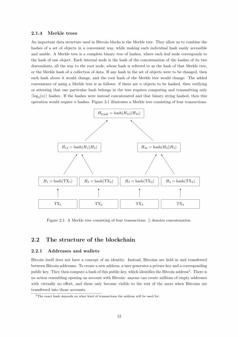
2.1.4 Merkle trees

An important data structure used in Bitcoin blocks is the Merkle tree. They allow us to combine the

hashes of a set of objects in a convenient way, while making each individual hash easily accessible

and usable. A Merkle tree is a complete binary tree of hashes, where each leaf node corresponds to

the hash of one object. Each internal node is the hash of the concatenation of the hashes of its two

descendants, all the way to the root node, whose hash is referred to as the hash of that Merkle tree,

or the Merkle hash of a collection of data. If any hash in the set of objects were to be changed, then

each hash above it would change, and the root hash of the Merkle tree would change. The added

convenience of using a Merkle tree is as follows: if there are n objects to be hashed, then verifying

or attesting that one particular hash belongs in the tree requires computing and transmitting only

dlog2(n)e hashes. If the hashes were instead concatenated and that binary string hashed, then this

operation would require n hashes. Figure 2.1 illustrates a Merkle tree consisting of four transactions.

Hroot = hash(H12||H34)

H12 = hash(H1||H2) H34 = hash(H3||H4)

H1 = hash(TX1) H2 = hash(TX2) H3 = hash(TX3) H4 = hash(TX4)

TX1 TX2 TX3 TX4

Figure 2.1: A Merkle tree consisting of four transactions. || denotes concatenation.

2.2 The structure of the blockchain

2.2.1 Addresses and wallets

Bitcoin itself does not have a concept of an identity. Instead, Bitcoins are held in and transferred

between Bitcoin addresses. To create a new address, a user generates a private key and a corresponding

public key. They then compute a hash of this public key, which identifies the Bitcoin address2. There is

no action resembling opening an account with Bitcoin: anyone can create millions of empty addresses

with virtually no effort, and these only become visible to the rest of the users when Bitcoins are

transferred into those accounts.

2The exact hash depends on what kind of transactions the address will be used for.

12

A user will generally have a Bitcoin wallet: a collection of Bitcoin addresses for different uses.

There exist several programs that manage Bitcoin wallets and will automatically generate and manage

multiple addresses for receiving and sending Bitcoins. This is partly for increased privacy, but also to

protect the user in the case of an unforeseeable break or improper implementation of the cryptographic

primitives used by Bitcoin3.

2.2.2 Transactions

When a user wishes to transfer Bitcoins from their wallet to another wallet they create a transaction

object. This transaction object is essentially an instruction to move Bitcoins from one address to

another, and is cryptographically signed with the private key corresponding to the sending address4.

This allows anyone with the complete transaction data to verify that this transaction was indeed

authorised by the user controlling that address: they will need to extract the public key, signature,

and sending address from the transaction, then cryptographically verify that the signature corresponds

to that public key and that the public key corresponds to the sending address. Transactions often

also include a transaction fee, which incentivises miners to include them in new blocks, discussed in

Section 2.2.3.

This cryptographical signing of transactions makes it possible to prove that a user authorised the

transfer of Bitcoins from their address to some other address without a central authority like a bank;

however, this does not stop that user from sending out a transaction spending Bitcoins they do not

really have or from sending a given Bitcoin multiple times, known as double spending5. To overcome

these two issues, there must exist some globally accessible ledger of all past transactions. In Bitcoin,

this ledger is the blockchain.

2.2.3 Blocks and the mining process

To prevent Bitcoins from being created out of thin air and to prevent double spending, Bitcoin

employs a decentralised database known as the blockchain which contains a full ledger of all confirmed

transactions. This database is incrementally updated through a process known as mining, discussed

in Section 2.2.3.

A block is a data structure containing two sections: a header and the data itself. The data section

consists of a list of transactions assembled in a Merkle tree whose hash is included in the header. The

header contains four pieces of information of interest to us: the hash of the last block in the chain, the

hash the Merkle tree of transactions in the block, the approximate timestamp at which the block was

mined, and an arbitrary integer called a nonce which is related to the mining process6. See Figure 2.2

for a simplified illustration of the block structure. Ignoring for the moment some additional fields in

the block header7, the hash is essentially calculated as

3The public key of a Bitcoin address need not be made public to the network until Bitcoins are spent, only a hashis made public. If a break in the elliptic curve cryptography were to be found, it would require the public key whichwould be hidden using this method.

4In reality, the underlying Bitcoin system uses a concept of inputs and outputs, which are manipulated by scriptsthrough a simple stack-based, non-Turing complete programming language. Transactions are hence a collection ofscripts that unlock inputs to create new “unspent” outputs. This is largely an artefact of the evolution of Bitcoin, andin practice, the vast majority of scripts adhere to a small set of standard formats.

5It is possible to create a type of digital currency without a blockchain that does not allow creating coins out of thinair; however, this is still prone to double spending. This idea is actually discussed in the original whitepaper [1] andprecedes Bitcoin.

6The block header also contains nBits, a measure of the mining difficulty, and nVersion, the block version, which isused in updates to the Bitcoin rules and protocol.

7The actual hash is hash(nVersion||hashPrevBlock||hashMerkleRoot||nTime||nBits||nNonce).

13

Hn = hash(Hn−1||Hroot||Timestamp||Nonce), (2.1)

where Hn is the hash of block n, Hroot is the hash of the Merkle tree of transactions as in

Figure 2.1, and || indicates concatenation. Figures 2.3 and 2.4 illustrate this relationship and how the

blockchain emerges from it.

Header

Block hash

Hash of previous block

Timestamp

Nonce

Merkle hash of data (Hroot)

Data

TX1

TX2

TX3

TX4

...

Figure 2.2: The simplified block data structure

Block n− 1

Block hash

Hash of block n− 2

...

Block n

Block hash

Hash of block n− 1

...

Figure 2.3: Links in the blockchain

Block n− 3 Block n− 2 Block n− 1 Block n

Figure 2.4: The blockchain

In order to mine valid blocks a miner must operate a full Bitcoin node. A full node is a server

that maintains a current copy of the full blockchain and validates new blocks as it receives them from

the network, conjoining them to its own replica of the chain. Without doing this, transactions that

it creates might be invalid due to being based on an outdated view of the balances of addresses. In

addition, blocks it mines will not be on the longest chain of blocks and will therefore be rejected by

other nodes on the network. For mining, the node needs to also receive and keep track of all currently

14

unconfirmed transactions being broadcasted onto the network in what is known as the memory pool,

or mempool.

Now to mine Bitcoins, the miner assembles a block template; a data structure identical to a block

but without a valid proof-of-work. To do this, it combines together a set of unconfirmed transactions

from its memory pool whose combined size is under the predefined size limit of a block. Ostensibly the

miner will choose transactions that maximise its reward from the transaction fees, incentivising users

to add higher fees into their transactions to receive priority service. Then to turn this block template

into a valid block, the miner attempts to find a proof-of-work hash, whose difficulty is defined by the

current mining difficulty. If the miner finds a valid hash, then it should swiftly attempt to broadcast

the newly mined block forward and get it propagated to the whole network before someone else finds

another block (unless attempting a selfish-mine strategy, or similar).

The mining difficulty is deterministically adjusted approximately every two weeks8 using the block

timestamps of the latest blocks in order to keep the arrival rate of new blocks being mined approxi-

mately constant at one new block every 10 minutes.

To incentivise miners to perform this work in validating transactions and advancing the blockchain,

miners are entitled to a block reward for finding a new block. When a miner successfully mines a

new block, they may include a transaction transferring new Bitcoins equivalent to the current block

reward to any addresses of their choosing. This transaction is called the coinbase transaction and

occurs first in each block. Currently this reward is at 12.5 Bitcoins per block and is set to half every

210000 blocks (which corresponds to approximately 4 years), until eventually being set to zero once

a total of 21 million Bitcoins have been mined. This incentive in turn means that there is economic

competition in providing the service, and there tends to be a large number of competing miners active

at any given time. The coinbase transaction contains an empty input that can be almost arbitrary9

and is commonly used by miners to include their mining signature, a string which advertises the miner

that mined that block.

According to the Bitcoin rules, miners should always mine on the longest chain they are aware

of. The length of a chain of blocks is given by the amount of chainwork on that chain: the expected

number of hashes required to produce the blocks in the current chain10. Not mining on top of this

longest chain would cause the blocks of the miner to not have as much chainwork as the longest chain,

and according to consensus rules, would be dropped by any other miners, effectively wasting the effort

of the miner mining on the wrong chain. This incentivises miners to quickly validate new blocks as

they receive them, and to mine on the longest chain.

Validating blocks is a simple process whereby a node verifies that the block contains a valid proof-

of-work, that the block header is correct, and that each transaction included in the block is valid

and correctly signed. The verification of digital signatures is the most computationally intensive in

comparison to the other verification tasks.

When two miners happen to find blocks at almost the same time, a fork in the blockchain can

occur, whereby a portion of the network believes that one of the blocks represents the current longest

chain of blocks, while another part of the network believes another block makes up the longest chain.

This is illustrated in Figure 2.5. This happens when a miner mines a block on the stale chain before

it learns about a new block, an artefact of the block propagation delay. In the case of a fork, each

8The mining difficulty is adjusted every 2016 blocks, which corresponds to 2 weeks if blocks occur every 10 minutes.9The latest version of the protocol requires this input to contain the block height, in order to stop two coinbase

transactions from being identical and hence having the same transaction hash, but other than that, this input scriptcan be arbitrary.

10To illustrate, suppose we had a list of integers between 0 and 264 − 1. One can compute the expected number ofindependent uniform random variables on the integers from 0 to 264 − 1 that need to be sampled to realise a list ofintegers which is uniformly bounded by the original list.

15

Block n− 2 Block n− 1

Block n

Block n′

Figure 2.5: A fork in the blockchain

miner will mine on the block they received first, ignoring other blocks at the same height. Eventually,

another miner will find a block on one of the branches and propagate it across the network, at which

point the miners mining on the wrong chain will see a longer chain, and switch to that chain, resolving

the fork. The leftover block is known as an orphan. This is illustrated in Figure 2.6.

Block n− 2 Block n− 1

Block n

Block n′ Block n+ 1

Figure 2.6: Resolution of a fork in the blockchain with the orphan block shaded

Forks can occur for other reasons as well, such as the selfish-mine strategy introduced in [4] and

explored further in [5] under the effects of propagation delay. In such a case, an adversarial miner

mines blocks on top of the longest chain, but instead of advertising new blocks as it finds them, hides

them and mines a longer, private chain. When that node then observes that the rest of the network

has mined another block, they reveal the next block in their private chain and attempt to quickly

flood the network with it. If they have superior infrastructure and can perform this faster than the

other node takes to propagate through the network, they can have their block be accepted instead of

the one mined by the rest of the network. This way, the adversarial miner gets a head start on new

blocks in their private chain, and can inflate their share of the rewards.

The mining process can be seen in two different ways. As one interpretation, it is a process whereby

a node is selected at random to process the next batch of transactions; with the probability of finding a

block being proportional to the processing power that that node contributes to the network. Another

interpretation of this process is that of a literal mining process, where any node doing work finds a

block (which grants them a reward) with some low probability, depending on how much effort is put

into the mining activity. However, the process is not equivalent to real mining, as the probability of

finding a block is adjusted periodically to make sure the total number of blocks is kept approximately

constant over time, despite fluctuations in total mining power.

2.2.4 51 % attacks and double spending

Controlling the mining process does not give the miner the ability to transfer arbitrary Bitcoins

between addresses. However, if one entity is able to dominate the mining process, they are able to

delay or even deny the confirmation of any transactions of their choosing, simply by not including

them in blocks. They may also engage in attacks known as double spending.

One version of double spending is when a miner with a sufficiently large proportion of mining

power creates a transaction and allows it to be confirmed, then takes possession of a good or service

paid for by that transaction; but immediately mines another block at the same height as the previous

block without that transaction. If they have a sufficiently large proportion of the hashing power on

16

the network, they can keep on producing blocks on top of this later block until it eventually takes

over the main blockchain, effectively erasing the transaction previously confirmed11. This is generally

known as a 51 % attack, referring to the fact that one entity requires over 50 % of mining power

to perpetually sustain this kind of attack on the blockchain. In the event of one entity controlling

the majority of mining power, they could always keep mining their own chain that would stay the

longest, and ignore any other blocks found by others, in practice keeping the network continuously

under their control. However, an entity need not control the majority of hashing power to succeed

with high probability in replacing a block; controlling the majority of hashing power just means that

they eventually succeed every time.

2.2.5 Application-Specific Integrated Circuits

Once a block template has been assembled and its corresponding header computed, the operation of

finding a small enough hash to satisfy the proof-of-work requirement is a fairly straightforward oper-

ation. It requires having the binary data for the header, computing a cryptographic hash, comparing

this to a threshold, and repeating this process while slightly modifying the header each time. Origi-

nally this work was done on commodity central processing units (CPU) found in desktop computers.

However, given the embarrassingly parallel12 nature of the hashing problem, it was soon discovered

that this was an ideal computation to be performed on a graphics processing unit (GPU), and soon

the rate at which a commodity GPU could compute hashes surpassed that of CPUs by several orders

of magnitude.

In the past few years, there has been increased work in offloading this computation to dedicated

hardware with circuits specifically engineered for the task. These application-specific integrated cir-

cuits (ASIC) drastically reduce the cost and energy requirements per hash, by removing a large portion

of hardware overhead. Due to the high research and development cost, as well as a high unit cost

associated with such dedicated hardware, the technology is developed by a handful of advanced com-

panies with the expertise to develop such technology and the capital to amortise these costs into their

operation. Even though this hardware is sold to the rest of the mining community, some fear that

this centralises control of the mining process. Some newer cryptocurrencies attempt to dwarf the de-

velopment of ASICs and force people to use commodity processors by introducing hashing algorithms

that cannot be easily computed via dedicated circuitry. This can be done, for instance by making a

hashing algorithm memory-hard, so that the proof-of-work requires large amounts of memory to be

quickly computed, or by making the proof-of-work space-hard, requiring for instance that the hash

accommodate information from a large number of random blocks in the history of the blockchain, so

that a device without the full blockchain cannot quickly compute it.

2.2.6 Mining pools

Due to the extremely low probability of finding a small enough hash to qualify for a new block, and

the historically ever-increasing aggregate hashing power of the network, the probability of finding a

block on any given piece of mining hardware over the lifetime of that hardware is small. In order to

reduce this risk, a number of mining pools have formed. These pools band together and aggregate

the hashing power from several miners, then share the rewards in order to reduce the variance in

11Generally the adversary will confirm into this alternate blockchain another transaction spending the same outputs,in order to make sure that transaction cannot be confirmed into the blockchain at any future time.

12In computer science, a problem is called embarrassingly parallel if it is trivial to perform that problem in parallelwhile introducing almost no overhead.

17

their mining operations13. This however, increases centralisation and means that these mining pools

generally control large proportions of mining power, often up to a third of the network. This is a

worrying fact, as mining pools are rarely run with much transparency and the entities controlling the

pool often get to single-handedly choose what gets accepted into a block and what does not.

2.2.7 The block size limit and SegWit transactions

In late 2017, an update called SegWit, or segregated witness, was activated on the Bitcoin network

to somewhat alleviate scalability issues as well as some security issues. Before this, the block size

limit for Bitcoin was defined to be one million bytes, and was measured as the size of the serialised

block. The SegWit update introduced an additional data section called “witness data” which is not

needed in determining the validity of certain parts of transactions, and thus can be discarded in some

cases. Due to this, the block size is now computed differently, in particular, parts of a transaction

that belong to the segregated witness data count for only one quarter of the size of normal data, and

a new unit, called a “weight” unit (or “weight byte”) was introduced. For normal transactions and

non-segregated witness data, one byte of data is equal to four weight units, whereas for segregated

witness data, one byte counts for only one weight unit. The block limit was also redefined and is now

4 million weight units.

2.3 The Bitcoin protocol

This section outlines the general Bitcoin protocol, but some details are specific to the Bitcoin Core

client as at version 0.17.1 [14].

2.3.1 Protocol messages

The Bitcoin network is an ad-hoc, peer-to-peer, decentralised network. Each entity willing to partic-

ipate in the mining or verification of transactions must operate a full node. The network protocol

is comprised of several short messages, transmitted on top of raw TCP sockets, by default on port

8333. These messages are preceded by a short message start sequence, followed by the message name,

the message data, and a checksum. There is only one class of messages, so there is no protocol-level

distinction between control messages and data messages. The protocol is a broadcast protocol: once

a transaction or block has been received by a computer, it attempts to quickly broadcast that object

to each of its peers that are missing it.

2.3.2 Nodes and peers

A computer connected to the Bitcoin network is called a node of the network. Two nodes that are

connected to each other are peers of each other. Hence the network consists of a set of nodes and a

set of peer-links.

13Interesting aside: when mining for a mining pool; it is not at first obvious how to prove to the pool that one isperforming a certain amount of mining work on behalf of that pool. Many mining pools have introduced innovativeways to prove this, such as a pay-per-share scheme where miners participating in the pool produce weaker “proofs” thatthey are mining for the pool: during the normal course of mining, a miner will inevitably stumble across block hashesthat are close to the real requirement but not quite low enough, such as differing by a few orders of magnitude. If theminers submit these to the mining pool which checks that the block is the one that the pool needs mined; then theycan both verify that the miner is working for that pool, as well as estimate the proportion of mining power contributedby that miner. Furthermore, once a miner finds a valid block, they are incentivised to send it to the pool, as they willget some proportion of the reward (possibly weighted by the proportion of shares submitted by them).

18

2.3.3 Peer discovery

A full Bitcoin node is a server connected to the Bitcoin network that maintains an up-to-date copy of

the full blockchain, while continuously receiving, verifying, and relaying transactions and blocks from

its peers.

When a new Bitcoin node joins the network, it must first establish an initial connection by finding

some peers. This is facilitated by a list of “good” nodes hardcoded into every release of the Bitcoin

client14. Upon starting afresh, a node will randomly pick some nodes from this list and establish

connections to them. Once a node has bootstrapped using this list of nodes, it will continuously grows

its list of good nodes by connecting to random nodes it receives from its peers and similarly advertise

the list to its peers. The sharing of information about nodes is done through the addr message, which

contains a list of address and port combinations of nodes, as well as a list of the capabilities of that

node.

When two nodes connect to each other, the procedure starts with a peer handshake. The connecting

node establishes a TCP socket to the second node, then sends a version message. This message

contains information about the node address and port, as well as its capabilities. The receiving node

in turn replies with a version message. Both nodes acknowledge they have received the version

message with verack messages, completing the version negotiation and connection establishment.

2.3.4 Control messages: version/verack, ping/pong, getaddr/addr

The protocol contains a selection of messages required for a node to control and maintain connections

and keep a current list of healthy peers.

The version and verack messages are used in the initial handshake, as outlined in the section

above. The version message contains a selection of information about the node, such as the protocol

version that node is running, the services it offers (such as whether it supports an upgraded, compact

way of transmitting blocks), the software name and the version that it is running, as well as network

information like the address and port of the sending and receiving nodes [14]. A verack message

acknowledges a previously received version message.

To confirm that a peer is still connected and responding, a node may send a ping message to that

node. This message contains only a random number used to label the corresponding pong message

that repeats the number, confirming that the peer is still connected and functioning.

In order for nodes to maintain a current list of healthy nodes, each node regularly sends an addr

message to each of its peers. This message contains a list of nodes, along with the majority of the

contents of their most recent version message. Additionally, a node may send a getaddr message to

its peers to request an addr message. During the course of its operation, a node regularly establishes

“feeler” connections to some of the nodes in its list of nodes not currently connected to, to check their

version information and make sure these nodes are healthy and ready to be connected to in case it

needs to connect to more peers.

2.3.5 Data messages: inv, getdata, tx, block, getheaders/headers

When a node wishes to inform a peer of blocks or unconfirmed transactions that it has but the peer

might not have, it sends an inv message. This contains a list of transaction or block hashes. The

14One of the core Bitcoin developers operates a crawler that records information on the various nodes available onthe network including their uptime and health. These are then occasionally filtered and compiled into the source codeas good bootstrapping nodes, that is, nodes good for fresh clients to connect to [19].

19

peer will then check its memory pool and database to decided whether or not it has these objects. To

request them, it sends a getdata message, asking for a list of objects from that peer.

Upon receiving a getdata request, a node replies with either a tx message to send a transaction,

or a block message to send a single block.

To accelerate the block propagation process, the protocol also contains a getheaders message

which requests only the header of a block, as well as the headers message which in turn only contains

the header of the block. This is vital for decreasing the block propagation delay.

The latest protocol versions contain some enhancements to block messages, known as compact

blocks, which allow a node to only transmit the parts of a block that their peer does not currently

have, achieved using bloom filters.

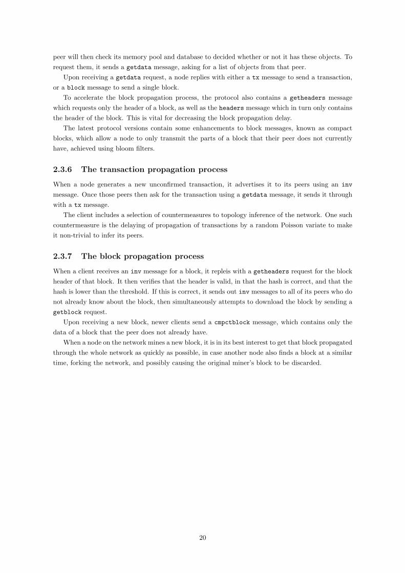
2.3.6 The transaction propagation process

When a node generates a new unconfirmed transaction, it advertises it to its peers using an inv

message. Once those peers then ask for the transaction using a getdata message, it sends it through

with a tx message.

The client includes a selection of countermeasures to topology inference of the network. One such

countermeasure is the delaying of propagation of transactions by a random Poisson variate to make

it non-trivial to infer its peers.

2.3.7 The block propagation process

When a client receives an inv message for a block, it repleis with a getheaders request for the block

header of that block. It then verifies that the header is valid, in that the hash is correct, and that the

hash is lower than the threshold. If this is correct, it sends out inv messages to all of its peers who do

not already know about the block, then simultaneously attempts to download the block by sending a

getblock request.

Upon receiving a new block, newer clients send a cmpctblock message, which contains only the

data of a block that the peer does not already have.

When a node on the network mines a new block, it is in its best interest to get that block propagated

through the whole network as quickly as possible, in case another node also finds a block at a similar

time, forking the network, and possibly causing the original miner’s block to be discarded.

20

Chapter 3

Data collection and the

bitcoin-crawler

In this chapter we give a detailed overview of the bitcoin-crawler and our setup for the experiment.

3.1 Overview

To analyse the underlying Bitcoin network, we set up an observational experiment to collect data about

the block propagation process. We provisioned servers in nine geographically separated datacentres

in locations around the world, which ran a custom software called bitcoin-crawler that we created

for this project.

In total, we provisioned 9 observational nodes, 1 master server, and 1 full Bitcoin node to collect

additional covariates. The full data collection system comprises of over 1000 lines of code and was

used to collect over 137 gigabytes of data.

Although the Bitcoin blockchain contains an immutable store of all data required to verify and

process transactions, it does not contain information about the process by which the network reached

consensus and how particular blocks were mined and propagated. In particular, we are interested in

the block propagation process and the path that newly mined blocks take to reach every network on

the node, as well as the delays associated with this. In a sense, this information is ephemeral. We

therefore needed to actively monitor the network by collecting and storing this information. In order

to get a comprehensive, real-time overview of the process, we needed to build a large system with

enough servers to receive data form the majority of nodes on the network.

This process was technically challenging both as it required an in-depth knowledge of the Bitcoin

protocol and software engineering, but also because it required the cost-effective deployment and

management of a number of servers that collected data in tandem in a large-scale, distributed manner.

This chapter outlines a tool called the bitcoin-crawler that we developed for the task, the system

of servers we deployed, and the data we collected, as well as some other aspects pertaining to the data

collection process.

3.2 The bitcoin-crawler

At the heart of the data collection was the bitcoin-crawler. This is a custom multi-threaded

software that we specifically developed for this project using the Python programming language. The

21

bitcoin-crawler imitates a full Bitcoin node by implementing a subset of the Bitcoin protocol but

contains custom logic to maintain connections to many more peers than a regular node, as well as

logging code to store the data of interest for later aggregation and analysis. The program uses the

python-bitcoinlib library by Todd [20] for some Bitcoin specific computations like serialisation.

The bitcoin-crawler starts by discovering its own IP addresses, which are required in connecting

to peers on the Bitcoin network. Each server was running on a dual-stack network supporting both

IPv4 and IPv6. The node does this by querying the master server which replies back with the

addresses.

In order to stay connected to the network, the bitcoin-crawler requires an up-to-date list of

addresses of possible peers to connect to similar to a normal Bitcoin node. Initially, it starts with the

same hard-coded list of well-known, good addresses embedded into the reference client (see Section

2.3.3 for further discussion). Once the bitcoin-crawler has bootstrapped itself through these nodes,

it learns about new addresses from its peers by periodically sending out addr messages.

When started, the program randomly chooses an address from this list of good addresses and

spawns a new thread to handle that address. The main thread keeps connecting to new random

addresses from this list whenever it needs to connect to more peers. After some experimentation on

how many peers we could connect to while keeping system load manageable, we chose to maintain

700 connections per server.

Once a new thread is spawned, that thread establishes a Bitcoin connection to its peer by per-

forming the initial handshake and agreeing on version parameters as specified in the protocol. When

the connection has been established, the thread performs three functions. The first is to log all ping

and pong messages, as well as messages advertising blocks (a subset of inv messages). This is the

data we collected and analysed in this project and is added to a global list of messages to be stored

to disk. The second function is to periodically send out an addr message to query that peer for new

addresses, which are then merged into the global list of potential addresses to connect to. Finally,

the thread maintains the connection by sending out and replying to necessary protocol messages. In

our implementation, this includes sending out inv messages every two minutes with our best guess of

the most recent block; as well as ping messages every thirty seconds to make sure the peer does not

disconnect due to inactivity. The thread also replies to incoming ping messages with a corresponding

pong message.

In order to not be marked as an outdated or stale node, we need to occasionally send out inv

messages with a current block hash to peers. However, as we did not maintain a full Bitcoin node

through the whole experiment and did not have current information on the blockchain on each server,

we had to guess it somehow. To do this, the bitcoin-crawler maintains a rolling buffer of the last

200 blocks observed and advertises the most common of those to its peers. After experimenting, this

seemed to work adequately.

The main thread contains a buffer for data to be saved to disk. When a thread needs to write to

this structure, it acquires a lock for it, and appends its data to the end of the buffer. Once this buffer

is full, the main thread acquires a lock on the structure and writes the data to disk and the buffer is

emptied.

Programming the bitcoin-crawler was a time-consuming task and took several weeks to finish.

Another approach would have been to take an existing Bitcoin client and operate full nodes, or to

modify an existing client to perform only the functions we require. However, the former would have

been too expensive as a full node has large overheads, demanding a large amount of processing power

and several hundred gigabytes of storage space; and the latter would have been a very time-consuming

endeavour and would most likely have taken longer to complete.

22

3.3 The global data collection system

In order to collect a sample of data from the global Bitcoin network and to get a comprehen-

sive overview of the underlying network and propagation process, we deployed servers running the

bitcoin-crawler at 9 geographically diverse locations around the world.

Each server was numbered from 1 to 9 for easy of identification. They were hosted on the Amazon

Web Services (AWS) Elastic Compute Cloud (EC2), on a variety of t2.nano and t3.nano instance

types and ran Ubuntu 18.04 LTS. The servers were assigned Elastic IP addresses, and a DNS hierarchy

hosted on Route 53 was set up to simplify server management. The servers were managed using SSH.

This information along with the AWS regions is summarised in Table 3.1 and Figure 3.1.

Northern Virginia

Northern California

Frankfurt

London

Seoul

Singapore

Mumbai

Sao Paulo

Sydney

Figure 3.1: Map showing locations of observational nodes

Number Location Region Instance type1 Northern Virginia us-east-1 t3.nano

2 Northern California us-west-1 t3.nano

3 Frankfurt eu-central-1 t3.nano

4 London eu-west-2 t3.nano

5 Seoul ap-northeast-2 t2.nano

6 Singapore ap-southeast-1 t3.nano

7 Mumbai ap-south-1 t2.nano

8 Sao Paulo sa-east-1 t3.nano

9 Sydney ap-southeast-2 t3.nano

Table 3.1: The locations used for data collection

A master server was provisioned to regularly copy data from each server into the master datastore,

as well as to serve information about IP addresses for the observational servers. In addition, the server

ran a PostgreSQL server and scripts to process the data.

3.4 Blockchain data and mining pools

To complement the real-time Bitcoin data, a full Bitcoin node was provisioned to extract data from

the blockchain itself. This was required to verify which blocks ended up being included in the final

blockchain and to classify blocks into mining pools through the coinbase transaction and the embedded

mining signature (refer to Section 2.2.3 and Section 2.2.6). The blockchain data was also used to

23

compute the size and number of transactions for each block, among other covariates. This data was

extracted by calling the Bitcoin Remote Procedure Call (RPC) interface and saving the results into

files that were processed by various scripts. In particular, the coinbase transaction input was extracted

from the block, decoded into UTF-8, and matched against a number of patterns known to identify

mining pools.

3.5 Cleaning of nonsensical data

Once the data had been collected, it was cleaned to remove any invalid data points.

The Bitcoin client has a rigorous battery of built-in techniques to disconnect from misbehaving

and adversarial peers. It maintains a tally of violations and once a peer passes a certain number of

violations, it is blocked. This is imperative for real nodes, as it is very easy to provision a server

with a reasonable budget that could connect to almost every node on the network and send spoofed

messages or poisoned data. If the client was unable to appropriately and sternly block these peers,

the whole network would be intimately exposed to a number of denial of service attacks.

Early on in our data collection we judged that implementing techniques to block nodes was un-

necessary for our program. This is because the vast majority of nodes on the network already block

these adversarial nodes, and so they have little incentive to spam the minority of custom nodes that

do not. Nevertheless, we found that some proportion of data was still nonsensical, and occasionally

we would encounter a fake block hash in our data.

We also removed orphaned blocks from our dataset (see Section 2.2.3). These are themselves of

interest when studying the mining process in general, but we did not include them in our dataset, as

they possibly have a different propagation pattern to non-orphaned blocks which we did not model.

To clean the collected corpus, we computed from the blockchain data a list of blocks that had been

accepted into the blockchain during the collection period. We then removed any data points that did

not overlap with this list. Approximately 16.5 % of data was removed in the cleaning step.

24

Chapter 4

The dataset

4.1 Overview of the dataset

In total, we collected in excess of 137 gigabytes of data. This chapter gives a brief overview of the

cleaned dataset presented through a discussion and some summary figures and tables.

Our main dataset contains one row for each inv message observed by an observational node

(see Section 2.3.5). Each block generally appears several times from different peers, and often even

several times per peer, as a peer may be connected to several of our observational nodes. In total,

the dataset contains approximately 20.6 million messages regarding 14810 unique blocks, which we

collected between November 2018 and March 2019.

Table 4.1 shows a sample from the main dataset. The block column contains the block hash and

has been truncated in the table for clarity. The time column is the time of that observations and

is recorded in Unix time, that is, in seconds since January 1st, 1970. The node and node location

columns correspond to values in Table 3.1 and identify which one of our nine observational nodes

received that message. Finally, the peer ip and peer port values contain the IP address and port of

the peer that sent the message.

The most common observation location was Northern Virginia. We do not know why there was

such a disparity in the number of observations by location, but we speculate it might be because of

a large number of nodes in that region with fast internet connections1. The proportions observed at

each location are shown in Figure 4.1.

Table 4.2 shows a sample of the blockchain data that complements the main dataset. This dataset

contains one row for each block that was mined during our experiment. Again, the block column

contains the block hash and has been truncated. The size column gives the real size of the block in its

1Virginia contains possibly the largest amount of cloud infrastructure in the world, due mianly to historical reasonsrelating to its proximity to Washington and funding from the United States Government.

block time node id node location peer ip peer port

0000...563df98 1542887007.19418 4 London 62.152.58.16 94210000...fda7919 1543748261.60442 9 Sydney 52.198.169.28 83330000...10c9e85 1544975472.21318 1 Northern Virginia 2a01:4f8:191:4174::2 83330000...f219fca 1547242755.84717 1 Northern Virginia 47.88.192.215 83330000...64dd0e6 1547487249.97776 4 London 108.56.233.194 83330000...ff3b14d 1547900706.97837 6 Singapore 117.52.98.78 83330000...11eeae7 1549261393.32542 6 Singapore 81.209.69.107 83330000...aa713e3 1549319396.6256 1 Northern Virginia 144.76.5.41 84330000...5cf4059 1550359795.0164 1 Northern Virginia 54.64.245.84 83330000...91f5404 1551099161.4188 1 Northern Virginia 185.186.209.210 8333

Table 4.1: A sample extract from the dataset

25

35.30 %

8.68 %

9.38 %

10.24 %

4.00 %

10.13 % 4.03 %

9.49 %

8.74 %

Northern Virginia

Northern California

Frankfurt

London

Seoul

Singapore

Mumbai

Sao Paulo

Sydney

Figure 4.1: Proportion of block messages by location

16.70 %

12.29 %

10.08 %

10.05 %

10.00 %

9.16 %

8.87 %8.79 %

4.36 %

3.86 %

2.99 %

2.84 %

BTC.com

AntPool

Unknown

F2Pool

Slush Pool

BTC.top

Poolin

ViaBTC

Huobi

dpool

Bitfury

BitClub

Figure 4.2: Proportion of blocks mined by mining pool

canonical encoding or when transmitted on the wire as a full block. weight is the weight of the block

as described in Section 2.2.7. The height column is the height of the block in the blockchain, and

time is the Unix time of the block as it appears in the block timestamp, which is often very inaccurate

26

block size weight height time nonce bits nTx pool

0000...f6048dd 1191087 3993369 550706 1542627049 1206282193 172a4e2f 1900 Slush Pool0000...b4373a9 154481 534173 553369 1544510774 3681510874 1731d97c 305 Unknown0000...f9dd7e9 649274 2359871 555601 1545843940 4123099930 17371ef4 648 Unknown0000...3984206 1283944 3993127 559626 1548178688 2688550637 172fd633 3133 AntPool0000...f1735ea 1262291 3993185 559645 1548188137 2421018921 172fd633 2524 BTC.com0000...ea10bc7 559802 1993133 562220 1549670573 2587934320 17306835 476 AntPool0000...18574e1 697494 2340000 562268 1549698426 1796028615 17306835 1700 Poolin0000...2316419 1288903 3993037 562793 1550026180 1918332176 172e6f88 2873 BTC.top0000...2df3348 1134403 3993103 564931 1551302350 2869178554 172e5b50 2040 BTC.com0000...a101cf8 1317204 3992916 565279 1551493180 1664069908 172e5b50 3273 Slush Pool

Table 4.2: A sample extract from the blockchain data

Dec Jan2019

Feb Mar

Date

0

25

50

75

100

125

150

175

200

Nu

mb

erof

blo

ckp

erw

eek

BTC.com

AntPool

Unknown

F2Pool

Slush Pool

BTC.top

Poolin

ViaBTC

Huobi

dpool

Bitfury

BitClub

Figure 4.3: Number of blocks mined by each pool over time

(see a discussion in Section 8.2). The nonce is the block nonce as discussed in Section 2.2.3. bits is

the mining difficulty threshold encoded using a special Bitcoin encoding scheme. Finally, nTx is the

total number of transactions in that block, and pool is the name of the mining pool that we believe

mined the block. Figure 4.3 shows the proportion of blocks mined by each mining pool.

To use this dataset, one would generally perform a join on the two tables; that is, for each

observation, one ought to match up the block hashes between the two tables to get the covariates

relating to that block from the blockchain table.

This is only a short overview of the dataset. For a further discussion of the data and trends within

it, see Part III, in which we explore several interesting phenomena and patterns we discovered in the

dataset.

4.2 Accompanying website and source code

We have made the data available online at https://bitcoin.aapelivuorinen.com/. This website

also includes other interesting complementary material, the source code for the bitcoin-crawler and

the fitting algorithm, and the final fits to be discussed in Part II.

27

Part II

Mathematical modelling

28

Chapter 5

Mathematical preliminaries

In this part, we develop the theory of parameter estimation for phase-type distributions via the EM-

algorithm and apply this to model the data obtained from our experiment. This chapter gives an

overview of the mathematical preliminaries required to understand our model. Chapter 6 discusses

the details of the method more deeply, in particular the computational aspects of the algorithm, and

in Chapter 7 we discuss how we applied this theory to fit phase-type distributions to block delay data

and discuss the results along with further mathematical extensions.

5.1 Continuous time Markov chains

We first briefly introduce a few basic concepts and results for Markov chains needed later on. Readers

familiar with the basic properties of continuous time-homogeneous Markov chains on finite state spaces

may skip this section. For proofs and a more rigorous, comprehensive treatment, see [21], [22], or [23].

The stochastic process underlying phase-type distributions is the continuous time Markov chain,

also known as the Markov jump process. In essence, a stochastic process is a Markov process if its

future trajectory depends only on the current state and not on any past state.

Definition 1 (Time-homogeneous Markov chains on finite state spaces). A cadlag stochastic process

Xtt≥0 which takes values in some finite set S, is a continuous time Markov chain if it satisfies the

Markov property:

P(Xtn = j | Xt1 = i1, . . . , Xtn−1

= in−1

)= P

(Xtn = j | Xtn−1

= in−1

)(5.1)

for all j, i1, . . . in−1 ∈ S, and every sequence 0 ≤ t1 < t2 < · · · < tn. We define the transition

probability for 0 ≤ s ≤ t as

pij(s, t) := P (Xt = j | Xs = i) . (5.2)

Furthermore, a Markov chain is called time-homogeneous if pij(s, t) = pij(0, t−s) for all i, j ∈ S, and

0 ≤ s ≤ t. We then simply write pij(t) := pij(0, t), so that pij(s, t) = pij(t− s).

In this thesis, we only consider time-homogeneous Markov chains on finite state spaces and assume

all Markov chains are such from now on. Note that some regularity conditions have been omitted from

the statements below, and they do not necessarily hold in generality for Markov chains with infinite

state spaces.

29

The evolution of a Markov chain is dictated by the transition semigroup and its corresponding

generator:

Definition 2 (Transition semigroup, generator, holding intensity). The transition semigroup of a

Markov chain, Xtt≥0 on state space S, is a family of matrices, PPP tt≥0, such that for a time t, PPP t

is the |S| × |S| matrix whose elements, [PPP t]ij are the transition probabilities, pij(t). The generator,

GGG, of a Markov chain is defined as

GGG := limh→0

1

h(PPPh − III). (5.3)

Finally, define the holding intensity, λi, of a state i ∈ SSS as λi := −Gii.

Lemma 3. The generator satisfies GGG111 = 000, and in particular, λi =∑j∈S\iGij.

Proof. See [21, p. 267].

Definition 4 (Embedded chain and holding times). Let Xtt≥0 be a Markov chain. We define the

embedded (discrete time) Markov chain Inn∈N and the holding times Si, i ∈ N as follows. Let

I0 := X0, and define S0 := inf t ≥ 0 |Xt 6= X0. Further define In+1 := XS0+···+Sn, and Sn+1 :=

inf t ≥ S0 + · · ·+ Sn |Xt 6= In. That is, In is the n-th state that Xt visits, and Sn is the time spent

in state In before jumping to another state.

An important property of the holding times is that they are exponentially distributed with pa-

rameter λi. We only state the result for S0, but it holds for any Si, with some more notational

clutter:

Lemma 5 (Exponentiality of holding times). Let Xtt≥0 be a Markov chain with generator GGG and

suppose X0 = i. Then S0 ∼ exp(λi) and for j 6= i, P (XS0= j) =

Gij

λi.

Proof. See [21, p. 259].

Definition 6 (Recurrent, transient and absorbing states). We call a state i ∈ S recurrent, if

P (∃n ≥ 1, XIn = i | X0 = i) = 1, that is, if the chain returns with almost surely to that chain

after leaving it. We call a state transient if it is not recurrent. Finally, a state is absorbing if

P (∃n ≥ 1, XIn 6= i | X0 = i) = 0, that is, if the chain does not leave that state once hitting it.

We now define the exponential of a matrix, defined by its Taylor series expansion:

Definition 7 (Matrix exponential). For a square matrix AAA, we define the matrix exponential,

eAAA :=∑n≥0

1

n!AAAn. (5.4)

It is not hard to show that the series converges for any square matrix, and so the exponential is

defined for all AAA [24, p. 160].

Theorem 8 (Matrix exponential as a solution to a differential equation). Define the differential

equation ∂∂yXXX(y) = AAAy with initial condition XXX(0) = III. Then the equation is uniquely solved by

XXX(y) = eAAAy.

Proof. See [24, p. 160].

Finally, we state the relationship between the transition semigroup and generator, which we need

later in fitting phase-type distributions to data:

30

Theorem 9. Subject to the boundary condition PPP 0 = III, we have

PPP t = eGGGt. (5.5)

Proof. See [21, p. 259].

5.2 Phase-type distributions

Phase-type distributions are a class of versatile probability distributions introduced by Erlang and

popularised by Neuts starting in [25]. Since their inception, they have enjoyed widespread adoption

and use in a range of stochastic modelling applications, in fields such as systems reliability modelling

[26, 27]; artificial intelligence and data mining [28, 29]; machine learning [30, 31]; finance [32]; insurance

pricing [33]; telecommunications [34]; population genetics [35]; maintenance engineering [36]; and

healthcare modelling [37, 38].

This popularity is due to several factors. In some sense, they are a natural extension from ex-

ponential and Erlang distributions, and often problems which can be analytically solved when one

assumes an exponential distribution are computationally tractable when replaced with a phase-type

distribution [39]. In many applied cases, phase-type distributions can also aid in interpretability, when

one assumes some kind of underlying state-based model. In addition to these desirable computational

properties, phase-type distributions are dense in the set of all distributions on the non-negative reals in

the sense of weak convergence (see Theorem 12), which further justifies their use as a parametrisation

of unknown distributions.

In this thesis, we used phase-type distributions as a tool to empirically fit distributions onto

observed delay data. This choice was somewhat arbitrary, although one could argue that given the

structure of the Bitcoin network, phase-type distributions provide a natural model for the delay

distribution. After all, the data are observations of hitting times of a very similar process to that of

a continuous time Markov chain, although the transition times across any given link or node are not

necessarily exponential, and the observations represent first hitting times of a group of observations.

For a full introduction to phase-type distributions, see [40], or [41].

Definition 10 (Phase-type distribution). Suppose Xtt≥0 is a continuous time Markov chain with

state space 0, . . . , p, where states 1, . . . , p are transient and state 0 is absorbing. Due to the absorbing

state at 0, the generator must then be of the form

GGG =

(0 000

ttt TTT

). (5.6)

We call TTT the phase-type generator and ttt the exit rate vector. Furthermore, let πππ be some row

vector defining the initial distribution on 1, . . . , p, and consider τ , the time until absorption of this

Markov chain:

τ = inf t ≥ 0 |Xt = 0 . (5.7)

We say τ is phase-type distributed with order p (or with p phases) with initial distribution πππ and

phase-type generator TTT , denoted τ ∼PH(πππ,TTT ).

31

We write Tvw := [TTT ]vw for v, w = 1, . . . , p, and sometimes refer to the v-th element of ttt as Tv0

when this simplifies notation. Note however that specifying TTT fully specifies ttt:

Theorem 11 (Properties of phase-type distributions).

1. ttt = −TTT111,

2. PPP t = eQQQt =

(1 000

111− eTTTt111 eTTTt

),

3. the distribution function is given by F (y) = 1− πππeTTTy111, and

4. the probability density function is given by f(y) = πππeTTTyttt.

Proof. For the first claim apply Lemma 3. For the second, apply Theorem 9 and the Taylor series

expansion in the definition of the matrix exponential after block partitioning the generator. The

second leads to the third as F (y) = P (Xy = 0) = πππ(111 − eTTTy111) = 1 − πππeTTTy111 as πππ is a probability

distribution. For the last claim, take the derivative: ∂∂y (1− πππeTTTy111) = −πππeTTTyTTT111 = πππeTTTyttt, by the first

claim.

We finish this section by stating a fundamental result of phase-type distributions, which justifies

using them for approximating arbitrary non-negative distributions.

Theorem 12 (Denseness of phase-type distributions). The class of phase-type distributions is dense

within the class of all distributions on the non-negative reals, in the sense of weak convergence.

Proof. See [41, p. 183], or [40, p. 149].

5.2.1 Examples of phase-type distributions

We now show some basic examples of well-known distributions formulated as phase-type distributions.

Example 13 (Exponential distribution). Consider a phase-type distribution with one phase with

T11 = λ and initial distribution πππ = eeeT1 . Then the phase-type distribution with parameters (πππ,GGG) has

the exponential distribution with parameter λ.

1 0λ

Figure 5.1: The underlying Markov chain of the exponential phase-type distribution

Example 14 (Generalised Erlang distribution). Suppose X1, . . . , Xn are independent exponential

random variables with rates λ1, . . . , λn, respectively. Then Y :=∑ni=1Xi is said to have the generalised

Erlang distribution, or Y ∼Erlangn(λ1, . . . , λn). If λi = λ for all i, then Y has the Erlang distribution,

denoted Y ∼Erlang(λ, n). Define πππ = eeeT1 and set

TTT =

−λ1 λ1 0 . . . 0

0 −λ2 λ2

......

. . .. . . 0

−λn−1 λn−1

0 . . . 0 0 −λn

, (5.8)

32

then PH(πππ,TTT ) has the Erlangn(λ1, . . . , λn) distribution.

1 2 . . . n 0λ1 λ2 λn−1 λn

Figure 5.2: The underlying Markov chain of the generalised Erlang phase-type distribution

5.2.2 Coxian distributions

The class of all phase-type distributions is quite large (with p(p+ 1)− 1 parameters for a model with

p phases), and as discussed later, this makes parameter estimation computationally difficult. To make

model fitting somewhat easier and reduce the parameter space, we restricted ourselves to working

with Coxian distributions, a rich sub-class of phase-type distributions:

Definition 15 (Coxian distributions). A random variable X is said to have the Coxian distribution,

if there exists TTT of the form

TTT =

−(λ1 + µ1) λ1 0 . . . 0

0 −(λ2 + µ2) λ2

......

. . .. . . 0

−(λn−1 + µn−1) λn−1

0 . . . 0 0 −λn

, (5.9)

such that with πππ = eeeT1 , X ∼PH(πππ,TTT ).

Note that this class of distributions only has 2p − 1 parameters. If we were to allow πππ to be

arbitrary, this would give rise to the class of generalised Coxian distributions as defined in [33] with

3p− 2 parameters.

1 2 . . . n 0λ1 λ2 λn−1 λn

µ1

µ2

Figure 5.3: The underlying Markov chain of a Coxian distribution

5.3 The expectation-maximisation algorithm

The expectation-maximisation algorithm, or the EM-algorithm, is an iterative algorithm for maximum

likelihood estimation when a model contains unobservable hidden variables, called latent variables.

Due to its reduced complexity and desirable computational properties, it is also sometimes used

33

for maximum likelihood estimation even in cases where there are no inherent latent variables, by

artificially formulating a problem as an incomplete-data problem [42]. The algorithm works by first

initialising the parameter estimates with some starting values, then finding the log-likelihood of the

full model given these parameter estimates and the observed data, then finally updating the estimates

to maximise this log-likelihood. The algorithm iterates by repeating these two steps, known as the

E- and the M-steps, respectively. Due to Jensen’s inequality, the algorithm steps through parameter

estimates with ever-increasing log-likelihoods, and under somewhat weak conditions converges to a

stationary point. However, care must be taken when applying the algorithm as this may be merely

a local maximum or a saddle point. See [43] for a systematic treatment of convergence results of the

EM-algorithm under a variety of conditions.

Suppose XXX is a random vector of the complete data of some experiment, and YYY is some observable

subset of the data, with yyy being the realisation of this observed data. Then under some unknown

parameters θθθ ∈ Ω of interest, our objective is to compute the maximum likelihood estimator, that is,

find θθθ that maximises the likelihood function L(θθθ) := f(yyy;θθθ). Our complete log-likelihood is defined

as

logLc(θθθ) := log f(xxx;θθθ). (5.10)

At the k + 1-th iteration, the EM-algorithm consists of performing the following two steps. The

first is the E-step, where we compute a function Q; the expectation of the complete log-likelihood at

θθθ under our current parameter estimates, θθθ(k), and given our observable data YYY = yyy,

Q(θθθ;θθθ(k)) := Eθθθ(k) (logLc(θθθ) | yyy) . (5.11)

Following this, in the M-step, we update our parameter estimates to some maximiser of Q, that

is,

θθθ(k+1) ∈ arg maxθθθ∈Ω

Q(θθθ;θθθ(k)). (5.12)

The General EM-algorithm, as discussed in [40], is a small modification in which one need only

choose some θθθ(k+1) such that Q(θθθ(k+1);θθθ(k)) ≥ Q(θθθ(k);θθθ(k)). This may be a much more attainable

task under computational constraints.

The EM-algorithm indeed monotonically increases our log-likelihood of the experiment, L(θθθ(k)),

at each step. To see this, let k(xxx | yyy;θθθ) be the conditional density of xxx given yyy under parameters θθθ,

and compute

logLc(θθθ) = log f(xxx;θθθ) (5.13)

= logL(θθθ) + log k(xxx | yyy;θθθ). (5.14)

Taking now the expectation given YYY = yyy under parameters θθθ(k+1), we have

34

Q(θθθ;θθθ(k)) = logL(θθθ) + Eθθθ(k) (log k(xxx | yyy;θθθ) | yyy) . (5.15)

So now

logL(θθθ) = Q(θθθ;θθθ(k))− Eθθθ(k) (log k(xxx | yyy;θθθ) | yyy) . (5.16)

Consider now the difference logL(θ(k+1)) − logL(θ(k)). The first part of this difference will be

non-negative by construction as we choose the next parameter estimate to satisfy Q(θθθ(k+1);θθθ(k)) ≥Q(θθθ(k);θθθ(k)). For the second part, let again θθθ ∈ Ω be arbitrary and note that the logarithm is concave,

so apply Jensen’s inequality,

Eθθθ(k) (log k(xxx | yyy;θθθ) | yyy)− Eθθθ(k)

(log k(xxx | yyy;θθθ(k)) | yyy

)= Eθθθ(k)

(log

k(xxx | yyy;θθθ)

k(xxx | yyy;θθθ(k))| yyy)

(5.17)

≤ logEθθθ(k)

(k(xxx | yyy;θθθ)

k(xxx | yyy;θθθ(k))| yyy)

(5.18)

= 0. (5.19)

The last equality follows from the definition of the pertinent expectation. Readers familiar with

machine learning will recognise Equation 5.17 as the negative of the Kullback-Leibler divergence of

the complete data given the observed data under θθθ(k) and the complete data given the observed data

under θθθ, and so the computation reduces to showing that Kullback-Leibler divergence is non-negative.

Therefore, each iterate of θθθ(k) increases the likelihood, L(θθθ(k)).

5.4 Fitting phase-type distributions to data

Our aim now is to apply the EM-algorithm for fitting phase-type distributions to data by estimating

the parameters πππ and TTT . We first construct the problem as a complete data experiment, and then

compute explicit formulas for the iterates to be computed at each step.

Consider the Markov process underlying a phase-type distribution of fixed order p. It is easy to

write down the maximum likelihood estimator for the parameters of the phase-type distribution if

we were able to observe the complete process. This would mean for each observation the number

of jumps, N until the chain reaches the absorbing state 0, the holding times S0, S1, . . . , SN−1 (with

SN = 0), and the embedded Markov chain I0, I1, . . . , IN−1. However, we only observe the absorption

time Y = S0 +S1 + · · ·+SN−1. Framed this way, the problem can naturally be seen as an incomplete

data problem, making it an apt application of the EM-algorithm.

Now consider a single observation x = ((i0, s0), (i1, s1), . . . , (in, sn)) of the complete data. The

sk, for k = 0, . . . , n are a realisation of an embedded Markov chain with transition probabilities

pjk = P (It+1 = k | It = j), as follows. For j, k = 1, . . . , p and j 6= k, we have

pjk =Tjkλj

, pj0 =tjλj. (5.20)

The ik, for k = 0, . . . , n on the other hand are simply realisations of exponential random variables

35

with rates λik . The complete likelihood for a single sample is then given by

Lc(πππ,TTT ;x) = f(x;πππ,TTT ) (5.21)

= πi0λi0e−λi0

s0pi0i1 · · ·λin−1e−λin−1

sn−1pin−10 (5.22)

= πi0e−λi0

s0Ti0i1 · · · e−λin−1sn−1Tin−10. (5.23)

Given now a sample of L independent observations of the underlying complete process, xxx =

(x1, . . . , xL), where superscripts denote the sample, we have the complete likelihood for that sample,

Lc(πππ,TTT ) =

L∏l=1

f(xl;πππ,TTT ) (5.24)

=

L∏l=1

πil0e−λ

il0sl0Til0il1 · · · e

−λiln−1

sln−1Tiln−10. (5.25)

Rearranging, grouping into phases, and performing some substitutions, we get the following form

for our complete likelihood:

Lc(πππ,TTT ) =

p∏v=1

πBvv

p∏v=1

eTvvZv

p∏v=1

p∏w=0w 6=v

TNvwvw . (5.26)

The substitutions are as follows: Bv =∑Ll=1 1il0=v is the total number of times that the processes

started from state v; Zv =∑Ll=1

∑nl

j=1 slj1ilj=v is the total time spent in state v; and Nvw =∑L

l=1

∑nl−1j=1 1ilj=v,ilj+1=w is the total number of transitions from v to w.

The Bv, Zv, and Nvw are a sufficient statistic for (πππ,TTT ) by the Fisher–Neyman factorization theo-

rem. Furthermore, we can explicitly though laboriously compute the maximum likelihood estimators

for πππ and TTT by standard theory. The computations are reserved for Appendix A. For v = 1, . . . , p,

and w = 0, . . . , p, v 6= w, the maximum likelihood estimators are given by

πv =Bvn, Tvw =

NvwZv

, Tvv = −p∑

w=0

Tvw. (5.27)

Since Bv, Zv and Nvw are a sufficient statistic, it suffices for the E-step to compute the expectation

of these under (πππ,TTT )(k) and given YYY = yyy. Also note that each of these statistics is a sum over the

sample, and the realisations in the sample are independent, so it is enough for each statistic to sum

the estimates for each sample, so we have

36

B(k+1)v =

L∑l=1

E(πππ,TTT )(k)

(Blv | yl

), (5.28)

Z(k+1)v =

L∑l=1

E(πππ,TTT )(k)

(Zlv | yl

), (5.29)

N (k+1)vw =

L∑l=1

E(πππ,TTT )(k)

(N lvw | yl

). (5.30)

Here again v = 1, . . . , p, w = 0, . . . , p, and v 6= w. The estimates for the parameters are updated

in the obvious way by substituting into Equation 5.27. Heavy computations are again recorded in

Appendix B. We define the matrix-valued convenience function

ΓΓΓ(y | πππ,TTT ) =

∫ y

0

eTTT (y−u)tttπππeTTTudu. (5.31)

Using this notation, our conditional expectations are given by

E(πππ,TTT ) (Bv | yyy) =

L∑l=1

πveeeTv eTTTylttt

πππeTTTylttt, (5.32)

E(πππ,TTT ) (Zv | yyy) =

L∑l=1

Γvv(yl | πππ,TTT )

πππeTTTylttt, (5.33)

E(πππ,TTT ) (Nv0 | yyy) =

L∑l=1

πππeTTTyl

eeevtv

πππeTTTylttt, (5.34)

E(πππ,TTT ) (Nvw | yyy) =

L∑l=1

TvwΓwv(yl | πππ,TTT )

πππeTTTylttt. (5.35)

5.5 Properties of the algorithm

One of the main drawbacks in fitting phase-type distributions with the EM-algorithm is that phase-

type distributions are heavily overparametrised [33] and exhibit a number of symmetries. This means

that there exist several parameter sets, (πππ,TTT ) that lead to the same distribution. For instance, simply

permuting the underlying state space of the Markov chain leads to p! parametrisations. In practice,

this translates to increased complexity in the search space, leading to slower convergence, and a higher

chance of converging to a local maximum or saddle point.

This algorithm has the convenient property that if some set of Tvw or πv are set to 0, then at

each iteration, that entry will remain 0. The advantage of this is that one can easily fit a sub-model

using the same algorithm, simply by initialising the algorithm with a matrix that has a specified

structure. For instance, to fit a Coxian distribution as in our case, one merely needs to initialise the

algorithm with a matrix whose entries are zero except on the diagonal and superdiagonal and a initial

distribution with π1 = 1. The EM-algorithm will then only ever lead to fits which are also Coxian.

Slight changes to the method lead to ways for fitting phase-type distributions to continuous distri-

butions, as well as to data that is censored (where only the interval that a data belongs in is observed

rather than the exact value), or a combination of fully observed and censored data. For details on

37

these techniques, see [44] and [33].

5.6 Akaike’s Information Criterion

Up to now, we have discussed fitting various phase-type distributions to empirical data for a fixed

number of phases, p. However, we have not yet discussed how to choose p, and how we can system-

atically compare fits with a different number of phases. If we were to simply fit several distributions

with varying p and compare them based on some measure of error from the data, then increasing p

would always decrease the error (in practice, convergence issues might cause larger models to lead

to worse fits), as a model with p − 1 parameters is a sub-model of one with p parameters. However,

this would not necessarily mean that we always find better approximations to the true underlying

distribution, but rather that we have so many free parameters that our model is fitting around the

randomness in our data. Simultaneously, we need to have a large enough p to capture the true shape

of the distribution and avoid underfitting through not capturing the true distribution well enough.

We need a method of model selection to balance out these two factors and get as close to the true

model as possible.

Although there are several criteria for model selection, we used Akaike’s information criterion

which amounts to choosing the model that minimises the number

AIC := 2k − 2 logL(θθθ;yyy) (5.36)

where k is the number of parameters in the model and θθθ is the maximum likelihood estimator, so

that logL(θθθ;yyy) is the maximum log-likelihood. We will not provide a full derivation of this criterion

for brevity. For a thorough treatment, see [45], [46], or [47]. Roughly speaking, if we assume there

exists some true distribution f that the underlying data originates from, then one can show that

the model which minimises AIC also minimises the Kullback-Leibler divergence between that model

and the true distribution. This result holds asymptotically in the number of samples under some

important technical assumptions.

5.7 MapReduce

The MapReduce paradigm is a method for parallelising a big data workflow, whereby data is first

partitioned into subsets, then handed off to worker queues where these workers apply some “mapping”

to them. Once the workers have finished, the results of the computations are finally merged, or

“reduced”. This is particularly useful in applications such as ours where there is a large number of

computations that can easily be performed in parallel, without results interacting with each other

except for in a final reduction step. We used the MapReduce paradigm to parallelise the algorithm

and decrease the fitting time on multi-core computers.

38

Chapter 6

Computational aspects of

phase-type fitting

In this chapter, we review some computational aspects of the EM-algorithm for fitting phase-type

distributions. We also discuss the implementation we used, and the modifications we made to existing

algorithms for our use-case to decrease the computational time on modern computing infrastructure.

The algorithm has two computationally heavy steps. The first is the computation of the integral

ΓΓΓ and the exponential eTTTy, and the second is when these two matrix-valued functions are evaluated

for each observation and are used to compute the contribution of that observation to Equations 5.32

to 5.35.

Generally, the first of the two is the computationally demanding step. However, as the number of

data points increases, as in our case, the second step also becomes increasingly difficult.

6.1 The integral ΓΓΓ

Traditionally, the most computationally difficulty part has been the computation of the matrix-valued

integral ΓΓΓ of dimension p × p to a sufficient level of accuracy, and to a smaller extent in computing

eTTTy, also of dimension p× p. As the number of phases, p, is increased, this task quickly becomes very

intensive. Most methods involve computing ΓΓΓ(y | πππ,TTT ) for a fine grid of y-values, then interpolating

between these when the expression needs to be approximated for a given y. This means that the

computational time of this step increases linearly with the maximum observed time.

Recall that ΓΓΓ is defined as

ΓΓΓ(y | πππ,TTT ) =

∫ y

0

eTTT (y−u)tttπππeTTTudu. (6.1)

A standard trick is to construct the block matrix

BBB =

(TTT tttπππ

000 TTT

), (6.2)

from which one can verify that

39

eBBBy =

(eTTTy ΓΓΓ(y | πππ,TTT )

000 eTTTy

). (6.3)

The calculation is reproduced in Appendix C. These kinds of integrals arise in several fields,

including differential equations, numerical methods, and control theory (where they are known as

Gramians). See [48] and [49] for an overview and [50] for a similar application.

This expression allows us to compute both eTTTy and ΓΓΓ by evaluating just one matrix exponential.

However, computing matrix exponentials and their error bounds in general is a very difficult problem.

See [51] for a discussion of several approaches to computing matrix exponential. Due to this, one

generally attempts to create specialised methods by exploiting additional structure in the problem

when high speed and accuracy are required. Unfortunately BBB is a 2p×2p-dimensional matrix without

much obvious structure. It is therefore reasonable to attempt to compute ΓΓΓ directly by exploiting its

structure; then compute eTTTy separately.

There exist several methods to compute ΓΓΓ, including through this combined matrix exponential, as

an ordinary differential equation, using standard quadrature methods, as well as using uniformisation

methods.

6.1.1 The EMpht.c program

The original method for fitting phase-type distributions via EM-algorithm was introduced by As-

mussen et al. in [39]. To accompany their paper, Olsson implemented an algorithm for computing

the estimates using an ordinary differential equation method in ANSI-C [52], which we refer to as

EMpht.c. In addition to ΓΓΓ, they defined the vector-valued helper functions

aaa(y | πππ,TTT ) = πππeTTTy, (6.4)

bbb(y | TTT ) = eTTTyttt. (6.5)

Using these, the conditional expectations become

E(πππ,TTT ) (Bv | yyy) =

L∑l=1

πvbv(yl | TTT )

πππbbb(yl | TTT ), (6.6)

E(πππ,TTT ) (Zv | yyy) =L∑l=1

Γvv(yl | πππ,TTT )

πππbbb(yl | TTT ), (6.7)

E(πππ,TTT ) (Nv0 | yyy) =

L∑l=1

tvav(yl | πππ,TTT )

πππbbb(yl | TTT ), (6.8)

E(πππ,TTT ) (Nvw | yyy) =

L∑l=1

TvwΓwv(yl | πππ,TTT )

πππbbb(yl | TTT ). (6.9)

Subject to the initial conditions aaa(0 | πππ,TTT ) = πππ, bbb(0 | TTT ) = ttt, and ΓΓΓ(0 | πππ,TTT ) = 000, the solutions to

these expressions can then be computed using a p(p + 2)-dimensional ordinary differential equation

with

40

∂

∂yaaa(y | πππ,TTT ) = aaa(y | πππ,TTT )TTT , (6.10)

∂

∂ybbb(y | TTT ) = TTTbbb(y | TTT ), (6.11)

∂

∂yΓΓΓ(y | πππ,TTT ) = TTTΓΓΓ(y | πππ,TTT ) + tttaaa(y | πππ,TTT ). (6.12)

The last derivative is by the Leibniz integral rule. Note that this is very similar to computing the

matrix exponential in Equation 6.3.

Their program solves these equations using a hardcoded fourth order Runge-Kutta method. These

equations are solved incrementally with some step size h up to the maximum value of the observation.

The conditional expectations are computed within this loop and each y-value is rounded down to the

nearest step. The new parameters are finally computed at the end of the routine.

We initially used the EMpht.c program to fit phase-type distributions to our data, but the program

was too slow to process our whole dataset, or even a substantial sample from it. In addition, some

of our data was very concentrated around zero, and had a long tail, which meant that stiffness of

the differential equation became an issue. This was hard to work around as the solver algorithm

was hardcoded and could not be tuned or changed. In particular, we found that ΓΓΓ(y,πππ,TTT ) would

occasionally evaluate to a negative value for some y, which then led to serious errors in the rest of the

computation, drastically worsening the convergence rate and hence fitting performance.

6.1.2 The EMpht.jl program

In [33], Laub wrote a new implementation of the algorithm using the Julia programming language,

and extended it in several ways. We will refer to this as the EMpht.jl program. The procedure

was modified to use the general OrdinaryDiffEq.jl library for computing ΓΓΓ, giving easy access to

a variety of stiff and non-stiff solvers. In addition to the original differential equation method, they

also implemented several alternative ways of computing ΓΓΓ for censored data, including quadrature

methods and a uniformisation method discussed next.

6.1.3 Uniformisation methods

Uniformisation methods for general Markov chains were introduced by Jensen, and have been used

extensively since then. The idea is the following.

If one defines a Poisson process Ntt≥0 with fixed rate λ, and independent from this a discrete

time Markov chain Inn∈N on a finite state space with transition matrix PPP , then one can show that

INtt≥0 is a continuous time Markov chain with generator λ(PPP −III) [53]. This is the idea of a Markov

chain subordinate to a Poisson process.

Uniformisation, also known as the randomisation technique1, is based on reversing this idea. We

call a continuous time Markov chain uniformisable if the diagonal entries of its generator are uniformly

bounded. In our case, as Markov chains have finite state spaces, this always holds. Suppose Xtt≥0

is a continuous time Markov chain with generator QQQ, and consider a Poisson process Ntt≥0 with

rate λ := supi λi where λi = −Qii is the negative of the i-th diagonal entry of the generator. Suppose

Inn∈N is an independent, discrete time Markov chain on the same state space with transition matrix

PPP := QQQ/λ+III. Now construct the Markov chain INtn∈N by subordinating this discrete time Markov

1Markov chains subordinate to a Poisson process can be thought of as discrete time Markov chains with randomisedjump times. The name originates from this.

41

chain, Inn∈N, to the Poisson process Ntt≥0. One can then show that again, INtn∈N is equivalent

to Xtt≥0 in the sense that they both have the same generator and all finite dimensional distributions

coincide [53].

This idea can be conceptualised as a clever way to simulate Xtt≥0 when one can only sample

from one homogeneous Poisson process Ntt≥0. Suppose the chain is initially in some state i ∈ S:

then the time until the next jump is distributed exponentially with rate equal to the holding intensity

λi, and the probability of transitioning to a different state j ∈ S, j 6= i is Qij/λi (cf. Lemma 5).

If the holding intensities were all equal, we could now simulate the whole of our Markov chain this

way. However, when the holding intensities are not all equal, one can achieve the same outcome by

sampling from an exponentially distributed random variable with intensity higher or equal to each

of the holding intensities, and then thinning this Poisson process. If we are in state i ∈ S, and

sample from a Poisson process with rate λ ≥ λi, then we first thin this process by ignoring the sample

and staying in the same state with probability Pii = 1 − λi/λ, and similarly to before, jumping to

another state j ∈ S, j 6= i with probability Pij = λi/λ × Qij/λi = Qij/λ. This is exactly how

the uniformisation technique works and the derivation shows how we arrive at the expression for the

transition matrix, PPP = QQQ/λ+ III. For a more in-depth overview on uniformisation, see [54] or [53].

We can use this formula to derive an expression for πππeQQQt as in [54] by conditioning on the number

of jumps before a time t. We get

πππeQQQt =∑n≥0

πππPPPn(λt)n

n!e−λt. (6.13)

The power of this method is that we can now explicitly express the truncation error in terms of a

Poisson tail probability,

∥∥∥∥∥πππeQQQt −N∑n=0

πππPPPn(λt)n

n!e−λt

∥∥∥∥∥∞

=

∥∥∥∥∥∑n>N

πππPPPn(λt)n

n!e−λt

∥∥∥∥∥∞

(6.14)

≤∑n>N

(λt)n

n!e−λt, (6.15)

this follows directly as πi ≤ 1. In general, this method is superior to differential equation methods

in computing transition probabilities for continuous time Markov chains [55].

In [55] and [56], Okamura implemented a complete uniformisation scheme for computing ΓΓΓ, based

on [57]. The first paper, [55] deals with non-censored data and [56] extended this to all cases treated

in the original papers of Asmussen [39] and Olsson [44].

In addition to tight guarantees on accuracy, Okamura proved that this improves the time com-

plexity of the computation by a factor of p, a significant improvement. However, this comes at the

cost of the time complexity depending on the number of data points.

In [33], the authors used EMpht.jl with an implementation of the uniformisation method by

Okamura, which they fitted to purely interval data. Their data consisted of a life table, that is, a

table showing for each age the probability of an individual of that age dying before reaching their

next birthday. Their data was therefore “binned” to bins of one year each, that is, they only observed

probability masses for yearly intervals. They only implemented these additional techniques for that

case. We did not adapt these techniques to the non-censored case as their time complexity increases

with the number of data points. By experimenting with the censored program, we found that the

42

time taken to compute solutions increased too quickly to handle all our data.

6.2 Our program

We based our final program on EMpht.jl by Laub, but modified it by implementing a hybrid approach

combining the original differential equation approach with a quadrature method as a backup.

As mentioned earlier, the differential equations were often stiff in our case. We experimented with a

number of stiff and non-stiff solvers, and eventually used an improved fifth order explicit Runge-Kutta

solving technique based on [58], as implemented in OrdinaryDiffEq.jl [59].

In addition to using a slightly improved solver, a special case was added to the procedure, where

if ΓΓΓ erroneously evaluated to an negative value for some observation, then ΓΓΓ(yl;πππ,TTT ) was recomputed

directly using the HCubature.jl library [60]. The library implements a quadrature algorithm based

on [61]. This is an adaptive algorithm for numerical integration that successively subdivides a hy-

perrectangle until a given tolerance is achieved [60]. This algorithm is substantially slower than the

other methods, but these problems arose in less than one percent of observations, so they did not

significantly affect running times. These were mostly either observations very close to the origin or

very close to the maximum observation. Furthermore, we found that the number of problems was

reduced as the algorithm progressed in iterations, indicating numerical instability in early iterations

which disappeared as the parameter estimates approached some maximum.

The original EM-algorithm, in both EMpht.c and EMpht.jl initialises πππ and TTT using uniform

random variables on the interval (0.1, 0.9), and following this, scales the values. πππ is scaled to be

a probability distribution, and TTT is scaled by multiplying by p/m where m is the median of the

observations. In our case, this led to a large number of issues with stiffness, so we further divided this

number by 10.

6.3 Computation of the conditional expectations

The computational aspects of the algorithm other than that of the various matrix integrals and

exponentials has mostly been ignored in prior work. However, as the number of data points increases,

just evaluating ΓΓΓ through some interpolation method and updating the parameter estimates in a single

thread of execution becomes computationally demanding.

The EMpht.jl program first solves the ordinary differential equation for ΓΓΓ, then for each observa-

tion yl, computes eTTTyl

, evaluates ΓΓΓ(yl;πππ,TTT ) (interpolating from the solution), and updates Equations

5.32 to 5.35 by adding the contribution of that observation. We made the trade-off to compute instead

a global solution to eTTTy up to the maximum of the yyy, then interpolate this for each observation. This

sacrificed some accuracy in the exponential, but allowed us to cache the solution for several time

values and interpolate between them, which sped up the algorithm overall.

We also implemented a straightforward way to parallelise this computations using a MapReduce

algorithm by applying standard techniques from computer science. In our instance, the mapping

operation was the computation of each individual observation’s contribution to the conditional expec-

tations in Equations 5.32 to 5.35, and the reduction step consisted of summing each of these together

and computing the new parameter estimates as by Equation 5.27. In the splitting step, the data

points were randomly assigned to queues, one queue for each worker, and each worker then tallied up

their contribution to the estimates. This procedure significantly decreased computational time, up to

several orders of magnitude for large instances.

43

Chapter 7

Phase-type fits to propagation

delays

In this section we fit phase-type distributions to the difference in block arrival times at Sydney and

Northern Virginia for those blocks that arrived first at Northern Virginia. We chose these locations

because blocks most commonly arrived at Northern Virginia first, and because Sydney is geographi-

cally far away from Virginia while also observing a large number of block arrivals. A histogram of the

arrival time differences is shown in Figure 7.1.

0.0 0.2 0.4 0.6 0.8 1.0

Delay in seconds

0.0

0.5

1.0

1.5

2.0

2.5

3.0

Figure 7.1: Histogram of arrival time differences between Northern Virginia and Sydney for blocksarriving first at Northern Virginia

44

7.1 Method

To perform the fits, we took the subset of blocks that were observed at both locations but arrived first

at Northern Virginia, of which there were 7759, or approximately 52.4 %, then subtracted the time of

observation at Northern Virginia from the time at which the block was first observed in Sydney.

We fitted Coxian phase-type distributions using our code for a varying number of phases, ranging

from one to six phases. Our stopping criterion was for the log-likelihood to stop increasing by more

than 1 × 10−6 on average over the past 100 iterations of the EM-algorithm. We only fitted to the

bottom 98 % of data, as this coincided almost exactly with 1 second, and the complexity of the

EM-algorithm grows with the maximum observation value, so fitting to the large outliers would have

caused the fits to take much longer to compute.

For each model, we ran the algorithm six times with random initial parameters. When fitting

with no more than four phases, the algorithm completed very quickly, took less than ten thousand

iterations, and always converged to the same estimates of TTT (the initial distribution is fixed for Coxian

distributions). With both p = 5 and p = 6, the code started taking longer and in two of the six runs,

failed to converge to the same value as the other four runs. Figure 7.2 shows the average running

times and number of iterations per run for successful runs.

1 2 3 4 5 6

p

0

2000

4000

6000

8000

10000

12000

14000

16000

Iter

ati

ons

0

2

4

6

8

10

Tim

ein

min

ute

s

Figure 7.2: Average running time and number of iteration per run for successful runs

It seems that the runs with six phases did not converge completely.

7.2 Model selection

We performed model selection using Akaike’s information criterion discussed in Section 5.6. The

number of parameters when fitting Coxian distributions is k = 2p− 1, so the AIC is given by

45

4p− 2− 2 logL(θθθ;yyy). (7.1)

We computed the AIC values for each model, which are shown in Figure 7.3. We stopped fitting

larger models after p = 6 as we found that the AIC had already started increasing at p = 4, and

because the fitting time was roughly exponential in the number of phases, making it difficult to

continue further.

1 2 3 4 5 6

p

−6500

−6000

−5500

−5000

−4500

−4000

−3500

−3000

−2500

AIC

3 4 5 6

p

−6300

−6280

−6260

−6240

−6220

−6200

−6180

AIC

Figure 7.3: AIC of models

The AIC values dropped quickly until p = 4, then slowly started growing again. We therefore

chose p = 4 as the best fitting model, which attained the minimum AIC of −6305.5.

7.3 Discussion

Figure 7.4 shows the fits for each value of p. For p = 1, we simply have an exponential distribution as

expected, and its rate parameter is approximately 3.18. The distribution for p = 2 at first resembles

the sum of two independent and identical exponentials, or an Erlang distribution with shape parameter

equal to 2. In fact, looking at its estimated phase-type generator, it is very close:

TTT 2 =

(−6.346 6.332

0 −6.346

). (7.2)

The sum of two exponentials would have the same form, but have the top right-hand element equal

to the negative of the diagonals.

We can also see that the fit gets better as p increase from 1 to 4, but that there is not much of

a difference between the fits with p = 4 to p = 6. Maybe the most noticeable difference is in the

behaviour near zero, where the fit with four phases differs slightly from the other two. The estimated

phase-type generator of the fit with p = 4 is

46

0.0 0.2 0.4 0.6 0.8 1.0

Delay in seconds

0.0

0.5

1.0

1.5

2.0

2.5

3.0p = 1

0.0 0.2 0.4 0.6 0.8 1.0

Delay in seconds

0.0

0.5

1.0

1.5

2.0

2.5

3.0p = 2

0.0 0.2 0.4 0.6 0.8 1.0

Delay in seconds

0.0

0.5

1.0

1.5

2.0

2.5

3.0p = 3

0.0 0.2 0.4 0.6 0.8 1.0

Delay in seconds

0.0

0.5

1.0

1.5

2.0

2.5

3.0p = 4

0.0 0.2 0.4 0.6 0.8 1.0

Delay in seconds

0.0

0.5

1.0

1.5

2.0

2.5

3.0p = 5

0.0 0.2 0.4 0.6 0.8 1.0

Delay in seconds

0.0

0.5

1.0

1.5

2.0

2.5

3.0p = 6

Figure 7.4: The phase-type distribution fits

TTT 4 =

−12.122 11.698 0 0

0 −12.121 11.210 0

0 0 −11.688 11.687

0 0 0 −11.691

. (7.3)

The parameter estimates were equal for each run. We can now also see why the differential

equations were stiff: there are several states that are almost instantaneous, where the underlying

Markov chain resides for a very short amount of time before jumping into the next state.

7.3.1 Basic statistics

The mean of our final fit with four phases is 0.3148, and its variance is 0.0304, its mode is 0.2896,

and its median is 0.2896. The 99-th percentile is at 0.832, which means that if the Bitcoin block

47

propagation delay in general followed this same distribution (discussed next), then 99 % of the nodes

on the network would receive a new block within 0.832 seconds.

7.3.2 Interval-censoring and censoring of the tail

Another approach to fitting phase-type distributions to this data would have been to bin the values to

intervals, say for each millisecond, then apply the interval-censored methods as in [33]. Given that our

data had 7923 observations, binning would most likely not have made a big difference in computational

speed, especially when the computationally intensive step was computed in parallel. However, when

fitting to larger datasets with lower requirements for accuracy, binning could be a worthwhile.

As discussed earlier, we computed fits to only the bottom 98 % of the data, cutting out the tail.

We could have included this data by treating it as right-censored and applying the methods in [44].

7.3.3 Interpretation as propagation delay

If we assume that the blocks that arrived first at Northern Virginia were mined close to Northern

Virginia, and that the arrival time there is close to the time at which the block was mined, then one

can interpret this fit as an approximation of the propagation delay between Northern Virginia and

Sydney. However, it is not obvious why these assumptions should be true, and it is hard to justify and

judge the extent to which this models real behaviour. We now propose a better way of interpreting

the results through an extension of the model.

7.3.4 Further extensions

Consider now a single block and the arrival times of that block at each of the observational locations.

We do not know the exact time at which this block was mined, but we can instead consider our

observation as consisting of XXX = YYY − M111 where YYY is the vector of true propagation delays and

M = minYYY . Let us stay within our framework of phase-type distributions by assuming that the

marginal distributions of YYY are phase-type distributed. This gives rise to two interesting models.

Assuming independence

Let us for a moment consider a simpler model and assume that the arrival times at each of the observa-

tional locations are independent and distributed identically. Then one can perform the computations

in Appendix B for the conditional expectations, but conditioning instead on YYY and M . In fact, by

the tower property of expectation, one can simply take the estimators for Bv, Zv, Nv0 and Nvw and

condition on YYY and M . We then need to apply the law of total probability and integrate over all the

values of the minimum, M . This gives a form similar to the standard E-step, but the expressions

include a second integral. For instance, for the conditional expectation of Blv with respect to the

observed times XXX = xxx, we get

E(Blv | xxx

)=

∫ ∞xl

eeeTv eTTTytttπv

πππeTTT (y−xl)ttt

πππeTTTytttdy. (7.4)

Here we are actually integrating with respect to yl, but have dropped the superscript for brevity.

Similarly, one can compute the other conditional expectations. For instance, for Zlv, we get

48

E(Zlv | xxx

)=

∫ ∞xl

∫ ∞0

eeeTv eTTT (y−u)tttπππeTTTueeevdu

πππeTTT (y−xl)ttt

πππeTTTytttdy. (7.5)

It may be possible to compute these integrals numerically, from which one could then compute the

maximum likelihood estimators for the parameters through an EM-algorithm as before. This would,

however, be very computationally demanding, and we have not attempted to do so yet.

Multivariate phase-type distributions

An even better model would be to not assume independence of the marginals at all, but rather assume

that YYY follows some kind of multivariate phase-type distribution.

Suppose YYY has n components. One idea would be to consider a Markov chain and choose n

absorbing subsets of the state space, such that once the chain has entered one of these subsets it

cannot escape. We then observe the times at which this Markov chain hits each of these n sets, giving

rise to the multivariate distribution for YYY . We need the subsets to have a non-empty intersection for

the marginals to be distributions. The marginal distributions are then all phase-type distributions.

Furthermore, one can see that the fully independent case is a submodel of this construction, for

instance by constructing the obvious Markov chain on the cartesian product of the state spaces of

the marginal phase-type distributions. It would be very interesting to study the dependent, joint

distribution of delays through this technique.

49

Part III

Exploratory Data Analysis and

Further Questions

50

Chapter 8

Patterns in the dataset

In this part, we explore the dataset further through a non-rigorous exploratory data analysis. Through

our research, we found several interesting patterns in the data that opened up a number of interesting

questions, but have not yet embarked on exploring or explaining them in detail. We present some

cursory thoughts and educated guesses on what might have caused them but attempt by no means a

thorough study of them.

8.1 Inter-arrival times of blocks

01/12/18 01/01/19 01/02/19 01/03/190

200

400

600

800

1000

Tim

esi

nce

last

blo

ckin

seco

nd

s

Figure 8.1: Daily rolling mean of inter-arrival times of blocks over the observed time period

As discussed in Section 2.2.3, the mining difficulty is adjusted about every two weeks to keep

the time between block at approximately 10 minutes. Figure 8.1 shows our observed inter-arrival

times, along with the objective of a 10 minute arrival time. In the first month of our experiment, the

51

inter-arrival times were on average higher than the 10 minute objective, then dipped for a few weeks

below it, and then finally stayed at approximately 10 minutes for the rest of the experiment. One

possible reason for these fluctuations is the exchange rate of Bitcoin, which dropped steadily from mid-

November until mid-December, which would incentivise some miners to stop mining if their operation

became unprofitable. Similarly, exchange rate increased again in the third week of December. When

miners stop mining, the total computational power of the network decreases and blocks become more

rare until the difficulty is adjusted to take this into account.

0 500 1000 1500 2000 2500

Difference to last block in seconds

0

50

100

150

200

250

300

350

Nu

mb

er

Figure 8.2: Distribution of inter-arrival times

A histogram of the inter-arrival times is shown in Figure 8.2. In the paper that introduce Bitcoin,

Nakamoto argues that the arrival process should be a Poisson process [1] which would lead to expo-

nential inter-arrival times. Our data fits to an exponential distribution with a mean of 606.2 quite

well. Bowden et al. however argue in [2] that this process is in fact not a Poisson process, and present

a refined model. We did not investigate how the arrival times fit to this model.

8.2 Difference between timestamp in the block header and

the arrival time

Figure 8.3 shows a histogram of the difference between the arrival time of a block and the timestamp

in the block header for each observed block. The Bitcoin protocol does not enforce strict rules on the

timestamp, such as requiring it to be in the past; however, there are some restrictions on how far it

can deviate from the median of previous blocks.

The majority of these differences are positive, meaning that the timestamp in the block header is

before the time at which we observed it. However, the magnitude of the difference is much higher than

what seems plausible under propagation delay. One explanation for this is if the mining pools require

52

−60 −40 −20 0 20 40 60

Difference in seconds

0

50

100

150

200

250

300

350

Ob

serv

atio

ns

Figure 8.3: Time difference between observed arrival time and the timestamp in block header

their miners to mine on the exact block template that has been sent by the pool, but recompute

and circulate a new block template infrequently. This would mean that the timestamp would only

be updated occasionally, leading to the observed behaviour of a large number of positive differences.

However, it is not clear why the timestamp wouldn’t be updated by miners in the pool independently.

It seems that it would be advantageous for mining pools to claim that blocks are mined further

apart than they really are in order to have the mining difficulty adjusted to be easier, hence giving

them higher rewards. However, this would cause a runaway effect where the “clock” of the blockchain

would forever have to advance faster than time in the real world. Although it seems that miners do

not do this, it may be that some miners include a timestamp in the future (giving a negative difference

in the graphs) in order to balance this out.

8.3 Empty and full blocks, size and weight

The weight of a block is a measurement of the size of the block, which accounts normal transactions

and SegWit transactions separately (see Section 2.2.7). In this section, we define a block as empty

if its weight is less than 50 thousand bytes, or 1.25 % of the maximum weight, which is four million

weight units. Similarly, we define a block as full if its size is no more than 50 thousand bytes from

the maximum weight limit, in other words, over 98.75 % full. Figure 8.4 shows the proportion of full

blocks, empty blocks, and those that are neither full nor empty. Empty blocks are discussed later

along with mining pools.

Blocks that are neither full nor empty seem to have an approximately uniform distribution. We

do not know why some miners create partially full blocks. An explanation for this would be if the

Bitcoin system processed all transactions and the memory pool was empty; however the network has

53

68.58 %

30.11 %

1.32 %

Full

Neither full nor empty

Empty

Figure 8.4: Proportion of full blocks, empty blocks, and blocks that are partially full

0.0 0.5 1.0 1.5 2.0 2.5 3.0 3.5 4.0

Block weight in millions of bytes

0

5

10

15

20

25

30

35

40

Nu

mb

er

Figure 8.5: Distribution of block weights for blocks that are neither full nor empty

been overloaded with transactions for several years now.

54

8.4 Block size and number of transactions

0 500 1000 1500 2000 2500 3000 3500 4000

Number of transactions

0.0

0.5

1.0

1.5

2.0

Blo

cksi

zein

million

sof

byte

s

Full block

Non-full block

Figure 8.6: Number of transactions versus actual block size

Figure 8.6 shows a figure of the number of transactions in a block versus its size. Blocks with a

block size larger than one million bytes contain witness data, which is not counted in the block size

limit equally, as discussed in Section 2.2.7. Non-full blocks show the expected trend of increasing

size with number of transactions. Transactions can be of different sizes, so this is not an exact linear

relationship. The majority of full blocks show a slight linear trend in size increasing from about 1 to

1.3 million bytes as the number of transactions increases. This linear trend could be explained by a

constant proportion of SegWit transactions.

The full blocks with only a few transactions, but with a large size are caused by very large SegWit

transactions. Those transactions close to one million bytes in size are large non-SegWit transactions.

Large transactions involve a large number of inputs and outputs, moving Bitcoins between very many

different addresses, but are all bundled in a single transaction. Such large transactions are sometimes

used by entities to obscure the origin of Bitcoins, akin to laundering money, often as a part of a

“coin laundry” service. A large transaction pools all the Bitcoins to be spent together (inputs), and

then splits them apart into all the outgoing addresses (outputs), without pairing inputs and outputs

together. This makes it very difficult to determine which addresses moved Bitcoins to which addresses.

8.5 Empty blocks and mining pools

Figure 8.7 shows the percentage of blocks that each pool mined that were empty. According to [62],

mining pools mine empty blocks during the time it takes them to validate the new block and create a

new block template. There are three delays associated with this: the first is the time it takes for the

mining pool’s control node to receive a new block in full after first receiving only the block header.

The second is the processing delay taken to validate the new block, remove the transactions in that

block from the memory pool of the control node, and create a new block template to mine on. The

third delay is the time it takes for that mining pool to distribute a new block template to its mining

55

BTC.com

Ant

Pool

Unk

nown

F2Poo

l

Slus

hPoo

l

BTC.to

p

Poolin

ViaBTC

Huo

bi

dpoo

l

Bitf

ury

BitC

lub

0.0

0.5

1.0

1.5

2.0

2.5

3.0P

erce

nta

ge

ofb

lock

s

Figure 8.7: Percentage of empty blocks by each mining pool

hardware and miners.

Most pools are open to the public: a miner downloads the software, then connects to the mining

pool that sends it the header of a block template to mine on. It would seem plausible that this software

were itself connected to the Bitcoin network, and could be programmed to start mining on an empty

block (which it could easily construct independently without needing a copy of the whole blockchain)

as soon as it observed a block header whose hash was correct. Independently of this, when the mining

pool operator would learn about the new block, they would construct a new header and distribute it to

all miners. Furthermore, this would remove the need for the miner and mining pool operator to have a

low latency connection. This hypothesis is supported by the fact that BTC.com and AntPool are both

very large pools open to the public, which presumably have a large number of miners distributed over

large geographical areas. F2Pool on the other hand, which has a small percentage of empty blocks,

is a small Chinese miner which is concentrated in a small geographical area. The large, distributed

pools have a large number of empty blocks, whereas the small, concentrated pool has a low number

of empty blocks.

8.6 Causes of delay

We attempted to explore the causes of propagation delay. To do this, we restricted ourselves to the

blocks that were first observed at Northern Virginia. We then computed the median time at which

each of the roughly 700 peers of the Northern Virginia observational location relayed the block to the

observational node. There are two reasons for using the median: the first is that the distribution is

56

BTC.com

Ant

Pool

Unk

nown

F2Poo

l

Slus

hPoo

l

BTC.to

p

Poolin

ViaBTC

Huo

bi

dpoo

l

Bitf

ury

BitC

lub

0

10

20

30

40

50

60

70P

erce

nta

geof

blo

cks

Figure 8.8: Percentage of full blocks by each mining pool

heavy tailed, so using the median is a better estimate of the centre than the mean. Secondly, the

median of the times it takes for a set of nodes to receive a block can be conveniently interpreted as

the time it takes for half of those nodes to reach consensus on the current state of the chain.

0.0 0.5 1.0 1.5 2.0

Block size in millions of bytes

0.0

0.1

0.2

0.3

0.4

0.5

0.6

0.7

0.8

Med

ian

del

ayin

seco

nd

s

Full block

Non-full block

Figure 8.9: Block size versus median delay of blocks

57

0 500 1000 1500 2000 2500 3000 3500 4000

Number of transactions

0.0

0.1

0.2

0.3

0.4

0.5

0.6

0.7

0.8

Med

ian

del

ayin

seco

nd

sFull block

Non-full block

Figure 8.10: Number of transactions versus median delay of blocks

Figure 8.9 shows this median as a function of the size of the block, and Figure 8.10 shows it as a

function of the number of transactions in the block. Note that the size and number of transactions in

a block are related, as discussed in Section 8.4.

The first figure does not seem to have a very clear trend, except that larger blocks take longer to

propagate. On the contrary, the latter figure shows a much clearer trend, and it seems that the delay

increases linearly with the number of transactions.

There are generally two sources of propagation delay: the network delay between nodes, and the

processing delay. The former is the time taken to relay the block from one node to another and latter

is the time it takes for a node to verify that a block header and all the transactions in that block are

valid.

These graphs seem to support the hypothesis that propagation delay is not caused by network

delays, but rather by processing delays, and in particular, in verifying transactions. One of the

most intensive computational steps in verifying a transaction is the verification of the cryptographic

signature within it. It would be interesting to compute the number of signatures to be verified in each

block, and plot these against the median delay, as each transaction does not always the same number

of signatures.

8.7 Delay and location

Figure 8.12 shows the total number of peers per country from whom we received block messages from.

We were interested in the role of geography on the propagation delay. We first computed for

each message the delay between that message and the first time we received a message about that

particular block. We then computed the median of this delay for each node. We removed nodes with

less than 10 messages. Finally, we performed a reverse geo-location based on the IP address of each

node and took the median of the values for each node in a country. Figure 8.13 shows this; note

the exponential scale. Figure 8.14 shows a histogram of all of these median delays. These are not

necessarily good measures summaries of the distribution of propagation delays, as the observations

58

BTC.com

Ant

Pool

Unk

nown

F2Poo

l

Slus

hPoo

l

BTC.to

p

Poolin

ViaBTC

Huo

bi

dpoo

l

Bitf

ury

BitC

lub

0.00

0.05

0.10

0.15

0.20

0.25

0.30

0.35

0.40M

edia

nb

lock

del

ayin

seco

nd

s

Figure 8.11: Median block delay for each mining pool

are heavily dependent.

59

Uni

ted

Stat

es

Ger

man

y

Chi

na

Fran

ce

Net

herla

nds

Can

ada

Uni

ted

Kin

gdom

Rus

sia

Japa

n

Sing

apor

e

Sout

hKor

ea

Aus

tralia

Oth

er0

500

1000

1500

2000

2500

Nu

mb

erof

pee

rs

Figure 8.12: Number of peers per country

102

101

100

10−1

Med

iand

elayin

second

s

Figure 8.13: Map of median delay by country

60

0.00 0.25 0.50 0.75 1.00 1.25 1.50 1.75 2.00

Median delay over all blocks

0

20

40

60

80

Figure 8.14: Histogram of median delay for nodes

61

Conclusion

In this thesis, we explored aspects of blockchain technology by studying the block propagation process

of Bitcoin. We created a tool and built a globally distributed data collection system to observe the

block propagation patterns of blocks on the network. We then used the EM-algorithm to fit phase-type

distributions onto a subset of the data. We discussed model selection and the quality of the fits, along

with further mathematical extensions to the method for more accurate models. Finally, we presented

an exploratory data analysis of the some of the data to shed some light on the patterns within it and

to open up further questions.

We made three contributions: an open dataset of cleaned, pre-processed Bitcoin network data

with covariates extracted from teh blockchain; a phase-type model for the block propagation delay;

and an improvement to the implementation of the EM-algorithm in [33] for large datasets. The data,

source code, and some additional complementary material is available on the accompanying website

at https://bitcoin.aapelivuorinen.com/.

62

Part IV

Appendices

63

Appendix A

Maximum likelihood estimators for

transition rates and initialisation

probabilities of a Markov chain

Our complete likelihood function is given in Equation 5.26,

Lc(πππ,TTT ) =

p∏v=1

πBvv

p∏v=1

eTvvZv

p∏v=1

p∏w=0w 6=v

TNvwvw . (A.1)

Therefore our complete log-likelihood, say `c, is given by

`c(πππ,TTT ) =

p∑v=1

Bv log πv +

p∑v=1

TvvZv +

p∑v=1

p∑w=0w 6=v

Nvw log Tvw (A.2)

=

p∑v=1

Bv log πv +

p∑v=1

p∑w=0w 6=v

(Nvw log Tvw − ZvTvw) . (A.3)

Note that πππ and TTT are decoupled in this equation, so it suffices to maximise with respect to each

variable individually. Computing first the derivative with respect to Tvw for v = 1, . . . , p, w = 0, . . . , p

with v 6= w, we get

∂`c(πππ,TTT )

∂Tvw=NvwTvw

− Zv. (A.4)

When this derivative vanishes, we have

Tvw =NvwZv

. (A.5)

We then need to find a probability vector πππ that maximises∑pv=1Bv log πv, subject to the prob-

ability constraint,∑pv=1 πv = 1. For this, let ψ be a Lagrange multiplier, and consider

64

L(πππ,BBB,ψ) =

p∑v=1

Bv log πv − ψ(

p∑v=1

πv − 1

). (A.6)

The derivatives are given by

∂L(πππ,BBB,ψ)

∂πv=Bvπv− ψ, ∂L(πππ,BBB,ψ)

∂ψ= 1−

p∑v=1

πv. (A.7)

Setting these to zero, and solving the linear system of equations gives us

πv =Bvn. (A.8)

Furthermore, all second order derivatives vanish except for

∂2`c(πππ,TTT )

∂T 2vw

= −NvwT−2vw ,

∂2`c(πππ,TTT )

∂πv= −Bvπ−2

v . (A.9)

These are both negative, and so the solution is a maximiser. Therefore, for v = 1, . . . , p, and

w = 0, . . . , p, v 6= w, the maximum likelihood estimators are given by

πv =Bvn, Tvw =

NvwZv

, Tvv = −p∑

w=0

Tvw. (A.10)

65

Appendix B

Computation of conditional

expectations

Consider a single realisation of the absorption time Y = y arising from a phase-type distribution with

parameters (πππ,TTT ), and let Ju be the state of the underlying continuous time Markov chain at time u.

We drop the extra superscripts and subscripts for clarity. First compute the conditional expectation

of Bv:

E (Bv | y) = P (J0 = v | Y = y) (B.1)

=P (J0 = v, Y ∈ dy)

P (Y ∈ dy)(B.2)

=P (Y ∈ dy | J0 = v)P (J0 = v)

P (Y ∈ dy)(B.3)

=eeeTv e

TTTytttπvπππeTTTyttt

. (B.4)

Similarly, we compute

E (Zv | y) = E(∫ y

0

1Ju=vdu | y)

(B.5)

=

∫ y

0

E(1Ju=v | y

)du (B.6)

=

∫ y

0

P (Ju = v | Y = y) du (B.7)

=

∫ y

0

P (Y ∈ dy | Ju = v)P (Ju = v)

P (Y ∈ dy)du (B.8)

=

∫ y

0

eeeTv eTTT (y−u)tttπππeTTTueeevπππeTTTyttt

du. (B.9)

Here we may interchange the integral and expectation as the integrand is non-negative. Before

embarking on the most difficult task of computing the conditional expectation of Nvw, let us compute

the easier conditional expectation of Nv0:

66

E (Nv0 | y) = P(Jy− = v | Y = y

)(B.10)

=P(Y ∈ dy | Jy− = v

)P(Jy− = v

)P (Y ∈ dy)

(B.11)

=tvπππe

TTTyeeevπππeTTTyttt

. (B.12)

Finally we compute the conditional expectation of Nvw. Consider first an approximation Nεvw

to this random variable for ε > 0 where we count the number of jumps from v to w at consecutive

windows of size ε. We have

E (Nεvw | y) = E

by/εc−1∑k=0

1Jkε=v,J(k+1)ε=w | y

(B.13)

=

by/εc−1∑k=0

P(Jkε = v, J(k+1)ε = w, Y ∈ dy

)P (Y ∈ dy)

(B.14)

=

by/εc−1∑k=0

P(Y ∈ dy | J(k+1)ε = w

)P(J(k+1)ε = w | Jkε = v

)P (Jkε = v)

P (Y ∈ dy)(B.15)

=

by/εc−1∑k=0

eeeTweTTT (y−(k+1)ε)ttteeeTv e

TTTεeeewπππeTTTkεeeev

πππeTTTyttt(B.16)

=1

πππeTTTyttt

by/εc−1∑k=0

εeeeTweTTT (y−(k+1)ε)ttteeeTv

(eTTTε − III

ε

)eeewπππe

TTTkεeeev. (B.17)

In the last step we used the fact that v 6= w so eeeTveeew = 0, and we have added nothing to the

equation. Now eTTTu is continuous, and we have

limε→0+

eTTTε − IIIε

= TTT . (B.18)

Combining these and interpreting the conditional expectation as an approximation of the Riemann

integral, we have as ε vanishes that

E (Nεvw | y)→ 1

πππeTTTyttt

∫ y

0

eeeTweTTT (y−u)tttTvwπππe

TTTueeevdu. (B.19)

Since this approximation is bounded above by Nvw and Nεvw → Nvw almost surely, we conclude

by the dominated convergence theorem for conditional expectation that

E (Nvw | y) =TvwπππeTTTyttt

∫ y

0

eeeTweTTT (y−u)tttπππeTTTueeevdu. (B.20)

Collating these results together gives us the conditional expectations

67

E (Bv | y) =πveee

Tv eTTTyttt

πππeTTTyttt, (B.21)

E (Zv | y) =1

πππeTTTyttt

∫ y

0

eeeTv eTTT (y−u)tttπππeTTTueeevdu, (B.22)

E (Nv0 | y) =πππeTTTyeeevtvπππeTTTyttt

, (B.23)

E (Nvw | y) =TvwπππeTTTyttt

∫ y

0

eeeTweTTT (y−u)tttπππeTTTueeevdu. (B.24)

Finally, to write them in cleaner form, define the matrix-valued function

ΓΓΓ(y | πππ,TTT ) =

∫ y

0

eTTT (y−u)tttπππeTTTudu. (B.25)

Then our conditional expectations take the form

E (Bv | y) =πveee

Tv eTTTyttt

πππeTTTyttt, (B.26)

E (Zv | y) =Γvv(y | πππ,TTT )

πππeTTTyttt, (B.27)

E (Nv0 | y) =πππeTTTyeeevtvπππeTTTyttt

, (B.28)

E (Nvw | y) =TvwΓwv(y | πππ,TTT )

πππeTTTyttt. (B.29)

68

Appendix C

Computations for the integral ΓΓΓ as

the exponential of a block matrix

Define

ΓΓΓ(y | πππ,TTT ) =

∫ y

0

eTTT (y−u)tttπππeTTTudu, (C.1)

BBB =

(TTT tttπππ

000 TTT

). (C.2)

We wish to show that

eBBBy =

(eTTTy ΓΓΓ(y | πππ,TTT )

000 eTTTy

). (C.3)

Firstly, by writing out the Taylor series expansion defining the matrix exponential (see Definition

7), we can easily verify that the diagonal blocks of eBBBy are equal to eTTTy, and the bottom left block is

zero. Let the remaining top right block be GGG(y), we then have

∂

∂yeBBBy = BBBeBBBy (C.4)

=

(TTT tttπππ

000 TTT

)(eTTTy GGG(y)

000 eTTTy

)(C.5)

=

(TTTeTTTy TTTGGG+ tttπππeTTTy

000 TTTeTTTy

). (C.6)

Apply the Leibniz integral rule to ΓΓΓ(y | πππ,TTT ), to get

∂

∂yΓΓΓ(y | πππ,TTT ) = tttπππeTTTy + TTT

∫ y

0

eTTT (y−u)tttπππeTTTudu (C.7)

= tttπππeTTTy + TTTΓΓΓ(y | πππ,TTT ). (C.8)

69

Recall from Theorem 8 that the matrix exponential, eBBBy may be computed as the unique solution

XXX(y) to the equation ∂∂yXXX(y) = BBBy with initial condition XXX(0) = III.

Combining this with the fact that ΓΓΓ(0 | πππ,TTT ) = 000, we have that ΓΓΓ(y | πππ,TTT ) satisfies the ordinary

differential equation arising from the top right-hand block of eBBBy. Therefore, we have GGG(y) = ΓΓΓ(y |πππ,TTT ), and so Equation C.3 holds, as required.

70

Bibliography

[1] Satoshi Nakamoto. Bitcoin: A peer-to-peer electronic cash system. 2009.

[2] R. Bowden, H. P. Keeler, A. E. Krzesinski, and P. G. Taylor. Block arrivals in the Bitcoin

blockchain. arXiv e-prints, page arXiv:1801.07447, Jan 2018.

[3] Pierre Goffard. Fraud risk assessment within blockchain transactions. 2018.

[4] Ittay Eyal and Emin Gun Sirer. Majority is not enough: Bitcoin mining is vulnerable. In Nicolas

Christin and Reihaneh Safavi-Naini, editors, Financial Cryptography and Data Security, pages

436–454, Berlin, Heidelberg, 2014. Springer Berlin Heidelberg.

[5] J. Gobel, H.P. Keeler, A.E. Krzesinski, and P.G. Taylor. Bitcoin blockchain dynamics: The

selfish-mine strategy in the presence of propagation delay. Performance Evaluation, 104:23 – 41,

2016.

[6] Yoad Lewenberg, Yoram Bachrach, Yonatan Sompolinsky, Aviv Zohar, and Jeffrey S. Rosen-

schein. Bitcoin mining pools: A cooperative game theoretic analysis. In Proceedings of the 2015

International Conference on Autonomous Agents and Multiagent Systems, AAMAS ’15, pages

919–927, Richland, SC, 2015. International Foundation for Autonomous Agents and Multiagent

Systems.

[7] Miles Carlsten, Harry Kalodner, S. Matthew Weinberg, and Arvind Narayanan. On the instability

of bitcoin without the block reward. In Proceedings of the 2016 ACM SIGSAC Conference on

Computer and Communications Security, CCS ’16, pages 154–167, New York, NY, USA, 2016.

ACM.

[8] Matthias Grundmann, Till Neudecker, and Hannes Hartenstein. Exploiting transaction accumu-

lation and double spends for topology inference in bitcoin. In Aviv Zohar, Ittay Eyal, Vanessa

Teague, Jeremy Clark, Andrea Bracciali, Federico Pintore, and Massimiliano Sala, editors, Fi-

nancial Cryptography and Data Security, pages 113–126, Berlin, Heidelberg, 2019. Springer Berlin

Heidelberg.

[9] Peter L. Juhasz, Jozsef Steger, Daniel Kondor, and Gabor Vattay. A Bayesian approach to

identify Bitcoin users. PLoS ONE, 13(12):e0207000, Dec 2018.

[10] T. Neudecker, P. Andelfinger, and H. Hartenstein. Timing analysis for inferring the topol-

ogy of the Bitcoin peer-to-peer network. In 2016 Intl IEEE Conferences on Ubiquitous In-

telligence Computing, Advanced and Trusted Computing, Scalable Computing and Commu-

nications, Cloud and Big Data Computing, Internet of People, and Smart World Congress

(UIC/ATC/ScalCom/CBDCom/IoP/SmartWorld), pages 358–367, July 2016.

71

[11] G. Zanzottera, P. Fragneto, and B. Rossi. A topological model for the blockchain. In 2018 IEEE

24th International Conference on Parallel and Distributed Systems (ICPADS), pages 1016–1021,

Dec 2018.

[12] Vincent Gramoli. From blockchain consensus back to byzantine consensus. Future Generation

Computer Systems, 2017.

[13] Hung Dang, Tien Tuan Anh Dinh, Dumitrel Loghin, Ee-Chien Chang, Qian Lin, and Beng Chin

Ooi. Towards Scaling Blockchain Systems via Sharding. arXiv e-prints, page arXiv:1804.00399,

Apr 2018.

[14] Bitcoin Core Developers. Bitcoin reference client. https://github.com/bitcoin/bitcoin, 2019.

[15] Erik De Win and Bart Preneel. Elliptic Curve Public-Key Cryptosystems — An Introduction,

pages 131–141. Springer Berlin Heidelberg, Berlin, Heidelberg, 1998.

[16] Certicom Research. SEC 1: Elliptic curve cryptography. 2009.

[17] Certicom Research. SEC 2: Recommended elliptic curve domain parameters. 2010.

[18] Adam Back. A partial hash collision based postage scheme.

http://www.hashcash.org/papers/announce.txt, 1997.

[19] Bitcoin core developers. Seeds utility. https://github.com/bitcoin/bitcoin/tree/176aa5a/contrib/seeds,

2018.

[20] Peter Todd. python-bitcoinlib. https://github.com/petertodd/python-bitcoinlib, 2019.

[21] Geoffrey Grimmett and David Stirzaker. Probability and Random Processes. Oxford University

Press, 2001.

[22] Masaaki Kijima. Continuous-time Markov chains, pages 167–241. Springer US, Boston, MA,

1997.

[23] Daniel W. Stroock. Markov Processes in Continuous Time, pages 99–136. Springer Berlin Hei-

delberg, Berlin, Heidelberg, 2014.

[24] Linear Systems and Stability of Nonlinear Systems, pages 145–224. Springer New York, New

York, NY, 2006.

[25] Marcel F. Neuts. Computational uses of the method of phases in the theory of queues. Computers

& Mathematics with Applications, 1(2):151 – 166, 1975.

[26] Marcel F. Neuts and Kathleen S. Meier. On the use of phase type distributions in reliability

modelling of systems with two components. Operations-Research-Spektrum, 2(4):227–234, Dec

1981.

[27] D. Peng, L. Fang, and C. Tong. A multi-state reliability analysis of single-component repairable

system based on phase-type distribution. In 2013 International Conference on Management

Science and Engineering 20th Annual Conference Proceedings, pages 496–501, July 2013.

[28] Adele Marshall, Sally McClean, Mary Shapcott1, and Peter Millard. Learning dynamic Bayesian

belief networks using conditional phase-type distributions. In Djamel A. Zighed, Jan Komorowski,

and Jan Zytkow, editors, Principles of Data Mining and Knowledge Discovery, pages 516–523,

Berlin, Heidelberg, 2000. Springer Berlin Heidelberg.

72

[29] Hakan L. S. Younes and Reid Simmons. Solving generalized semi-Markov decision processes using

continuous phase-type distributions. pages 742–748, 01 2004.

[30] Adele H. Marshall and Barry Shaw. Computational learning of the conditional phase-type (c-ph)

distribution. Computational Management Science, 11(1):139–155, Jan 2014.

[31] L. J. Perreault, M. Thornton, R. Goodman, and J. W. Sheppard. A swarm-based approach to

learning phase-type distributions for continuous time Bayesian networks. In 2015 IEEE Sympo-

sium Series on Computational Intelligence, pages 1860–1867, Dec 2015.

[32] Alexander Herbertsson. Modelling default contagion using multivariate phase-type distributions.

Review of Derivatives Research, 14(1):1–36, Apr 2011.

[33] Søren Asmussen, Patrick J. Laub, and Hailiang Yang. Phase-type models in life insurance: Fitting

and valuation of equity-linked benefits. Risks, 7(1), 2019.

[34] M. K. Boroujeny, Y. Ephraim, and B. L. Mark. Phase-type bounds on network performance. In

2018 52nd Annual Conference on Information Sciences and Systems (CISS), pages 1–6, March

2018.

[35] Asger Hobolth, Arno Siri-Jegousse, and Mogens Bladt. Phase-type distributions in population

genetics. arXiv e-prints, page arXiv:1806.01416, Jun 2018.

[36] C. Wang, Y. Zhang, G. Wang, and L. Wang. Reliability modeling of protection system based

on phase-type distribution. In 2012 3rd IEEE PES Innovative Smart Grid Technologies Europe

(ISGT Europe), pages 1–5, Oct 2012.

[37] Adele H. Marshall and Sally I. McClean. Using Coxian phase-type distributions to identify patient

characteristics for duration of stay in hospital. Health Care Management Science, 7(4):285–289,

Nov 2004.

[38] Vincent A Knight and Paul R Harper. Modelling emergency medical services with phase-type

distributions. Health Systems, 1(1):58–68, Jun 2012.

[39] Søren Asmussen, Olle Nerman, and Marita Olsson. Fitting phase-type distributions via the EM

algorithm. Scandinavian Journal of Statistics, 23(4):419–441, 1996.

[40] Mogens Bladt and Bo Friis Nielsen. Estimation of Phase-Type Distributions, pages 671–701.

Springer US, Boston, MA, 2017.

[41] Phase-Type Distributions, pages 169–184. Springer Netherlands, Dordrecht, 2005.

[42] Shu Kay Ng, Thriyambakam Krishnan, and Geoffrey J. McLachlan. The EM Algorithm, pages

139–172. Springer Berlin Heidelberg, Berlin, Heidelberg, 2012.

[43] C. F. Jeff Wu. On the convergence properties of the EM algorithm. Ann. Statist., 11(1):95–103,

03 1983.

[44] Marita Olsson. Estimation of phase-type distributions from censored data. Scandinavian Journal

of Statistics, 23(4):443–460, 1996.

[45] H. Akaike. A new look at the statistical model identification. IEEE Transactions on Automatic

Control, 19(6):716–723, December 1974.

73

[46] Ritei Shibata. Statistical Aspects of Model Selection, pages 215–240. Springer Berlin Heidelberg,

Berlin, Heidelberg, 1989.

[47] Kenneth P. Burnham and David R. Anderson, editors. Information and Likelihood Theory: A

Basis for Model Selection and Inference, pages 49–97. Springer New York, New York, NY, 2002.

[48] C. Van Loan. Computing integrals involving the matrix exponential. IEEE Transactions on

Automatic Control, 23(3):395–404, June 1978.

[49] F. Carbonell, J.C. Jımenez, and L.M. Pedroso. Computing multiple integrals involving matrix

exponentials. Journal of Computational and Applied Mathematics, 213(1):300 – 305, 2008.

[50] Sophie Hautphenne and Mark Fackrell. An EM algorithm for the model fitting of Markovian

binary trees. Computational Statistics & Data Analysis, 70:19 – 34, 2014.

[51] C. Moler and C. Van Loan. Nineteen dubious ways to compute the exponential of a matrix,

twenty-five years later. SIAM Review, 45(1):3–49, 2003.

[52] Marita Olsson. The EMpht-programme, June 1998.

[53] Donald Gross and Douglas R. Miller. The randomization technique as a modeling tool and

solution procedure for transient Markov processes. Operations Research, 32(2):343–361, 1984.

[54] W.K. Grassmann. Transient solutions in markovian queueing systems. Computers & Operations

Research, 4(1):47 – 53, 1977.

[55] Hiroyuki Okamura, Tadashi Dohi, and Kishor S. Trivedi. A refined EM algorithm for PH distri-

butions. Performance Evaluation, 68(10):938 – 954, 2011.

[56] Hiroyuki Okamura, Tadashi Dohi, and Kishor S. Trivedi. Improvement of expecta-

tion–maximization algorithm for phase-type distributions with grouped and truncated data. Ap-

plied Stochastic Models in Business and Industry, 29(2):141–156, 4 2013.

[57] Andrew Reibman and Kishor Trivedi. Numerical transient analysis of Markov models. Computers

& Operations Research, 15(1):19 – 36, 1988.

[58] Ch. Tsitouras. Runge–Kutta pairs of order 5(4) satisfying only the first column simplifying

assumption. Computers & Mathematics with Applications, 62(2):770 – 775, 2011.

[59] OrdinaryDiffEq.jl. https://github.com/JuliaDiffEq/OrdinaryDiffEq.jl, 2019.

[60] Steven G. Johnson. HCubature.jl. https://github.com/stevengj/HCubature.jl, 2019.

[61] A.C. Genz and A.A. Malik. Remarks on algorithm 006: An adaptive algorithm for numerical

integration over an N-dimensional rectangular region. Journal of Computational and Applied

Mathematics, 6(4):295 – 302, 1980.

[62] Pascal Gauthier. Why do some Bitcoin mining pools mine empty blocks?

https://bitcoinmagazine.com/articles/why-do-some-bitcoin-mining-pools-mine-empty-blocks-

1468337739/, 2016.

74