Comparison of Support Vector Machine and Back ...aircconline.com/ijaia/V1N3/0710ijaia3.pdfComparison of Support Vector Machine and Back Propagation Neural Network in Evaluating the

International Journal of Artificial Intelligence & Applications (IJAIA), Vol.1, No.3, July 2010

DOI : 10.5121/ijaia.2010.1303 31

Comparison of Support Vector Machine and

Back Propagation Neural Network in

Evaluating the Enterprise Financial Distress

Ming-Chang Lee1 and Chang To2

1Department of Information Management, Fooyin University ,Taiwan

[email protected] 2Department of Information Management Shu-Te University, Taiwan

[email protected]

ABSTRACT

Recently, applying the novel data mining techniques for evaluating enterprise financial distress has

received much research alternation. Support Vector Machine (SVM) and back propagation neural (BPN)

network has been applied successfully in many areas with excellent generalization results, such as rule

extraction, classification and evaluation. In this paper, a model based on SVM with Gaussian RBF

kernel is proposed here for enterprise financial distress evaluation. BPN network is considered one of

the simplest and are most general methods used for supervised training of multilayered neural network.

The comparative results show that through the difference between the performance measures is marginal;

SVM gives higher precision and lower error rates.

KEYWORDS

Enterprise Financial Distress, Support Vector Machines, Back-Propagation Neural Network, Gaussian

RBF Kernel

1. INTRODUCTION

The financial crisis means that business enterprise loses the ability of payment, has no capability

to play expired liability or expenses and appears asset value less than issued debt. Once the

enterprise occur financial crisis, it will bring great loss for executive and financial institution.

Financial distress prediction is of interest not only to managers but also to external stakeholders

of company. Gestel et al. [10] observed corporate bankruptcy cause substantial losses to the

business community and society as whole. For financial institutions, poor decision when

granting credit to corporations in either losing potentially valuable clients or incurring

substantial capital loss when the client subsequently defaults.

From the late 1980s, the machine learning techniques in the Artificial Intelligence (AI) area,

such as Artificial Neural Network (ANN) were applied to financial distress prediction studies [1]


32

[4] [5] [6] [13] [14] [15] [23]. Singh et al.,[24] used ANN to the fault tolerant behavior.

Chakraborty and Sharma [2] used Radial Basis Function Neural Network (RBF), multiplayer

Perception (MLP), Self-Organized Competition (SOC) and Support Vector Machines (SVM) to

examine credit evaluation capability. Currently, there has been a considerable interest in ANN

because enterprise index with credit risk exist non linear relationship. It confirms that the

effect of credit risk prediction using ANN is good than using MDA [18][20][23]. But, a

potential drawback of ANN methods is that they need man-made adjustability in calculated

process. The calculated processes consume labor power and time.

In order to improve the performance of enterprise financial distress evaluation, many artificial

intelligence methods such as neural network have been widely used. These methods are based

on an empirical and have some disadvantages such as local optimal solution, low convergence

rate, and epically poor generalization when the number of class samples is limited [21]. In

1990s, Support Vector Machine (SVM) was introduced to cope with the classifications and the

small number of quadratic programming in SVM training is applied. Fan and Palaniswami [8]

applied SVM to select the financial distress predictors. SVM was introduced by vapnik in the

late 1960’s on the foundation on statistical learning theory [19]. SVM is a set of related

supervised learning methods used for classification and regression. O’Neill and Penm [12] use

SVM algorithm testing Standard & Poor (S&P) publisher credit data, which provide credit safe

information to an investor. SVM is very effective method for general purpose pattern

recognition based on structural risk minimization principles.

This paper is organized as follows: Section 2 deals with the foundations of support vector

machine. In this section we will consider the problem of linear and nonlinear decision

function Section 3 deals with back-propagation neural network. In section 4, we have a

procedure for Enterprise Financial Distress evaluation, and give an illustration. It help in

understanding of this procedure, a demonstrative case is given to show the key stages involving

the use of the introduced concepts. Section 5 is conclusion.

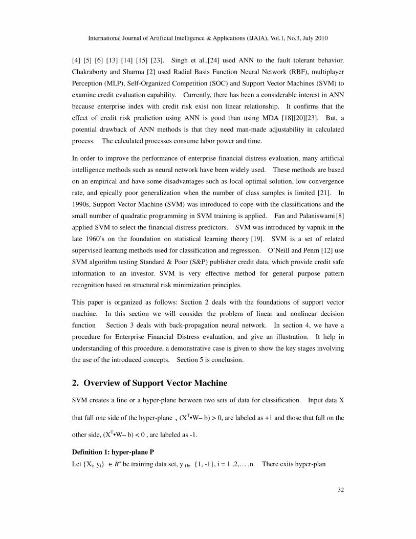
2. Overview of Support Vector Machine

SVM creates a line or a hyper-plane between two sets of data for classification. Input data X

that fall one side of the hyper-plane，(XT•W– b) > 0, arc labeled as +1 and those that fall on the

other side, (XT•W– b) < 0 , arc labeled as -1.

Definition 1: hyper-plane P

Let {Xi, yi} nR∈ be training data set, y i∈ {1, -1}, i = 1 ,2,… ,n. There exits hyper-plan


33

P ={X nR∈ ｜XT•W+ b = 0} (1)

The training data set satisfies the following con

1, 1T

iiX W b y+ ≥ = (2)

1, 1T

iiX W b y+ ≤ − = −

It can be written as

( 1) 0T

i iy X W b+ − ≥

Definition 2: hyper-plane p and p+ −

Let {Xi, yi} nR∈ be training data set, y i∈ {1, -1}, i = 1 ,2,… ,n.

p+ ={X nR∈ ｜ T

iX W + b =1} (3)

p− ={X nR∈ ｜ T

iX W + b = -1}

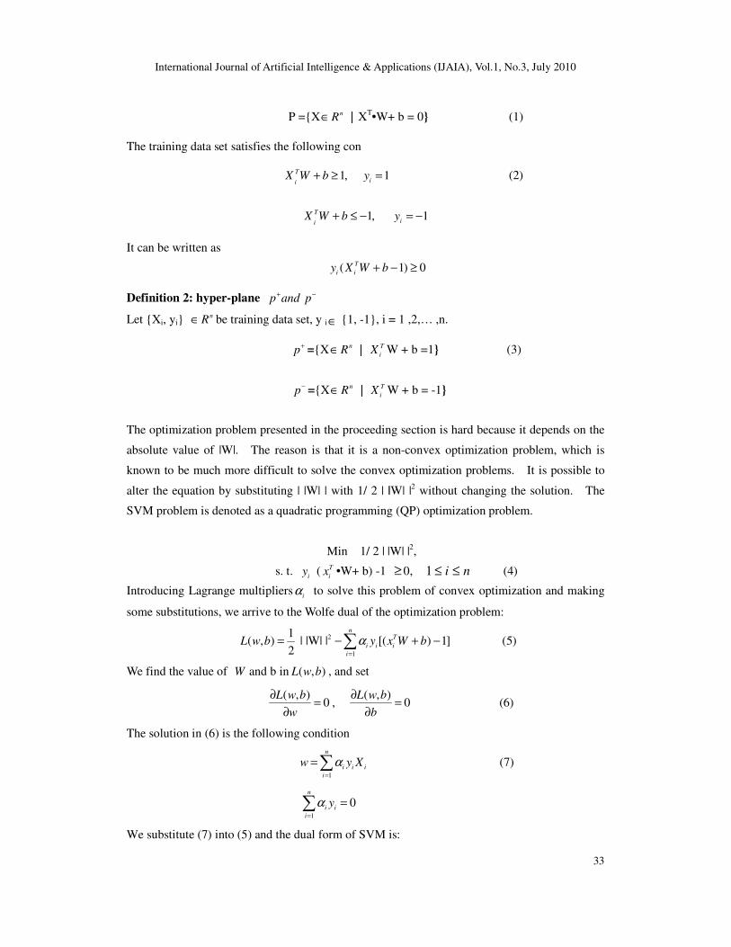
The optimization problem presented in the proceeding section is hard because it depends on the

absolute value of |W|. The reason is that it is a non-convex optimization problem, which is

known to be much more difficult to solve the convex optimization problems. It is possible to

alter the equation by substituting | |W| | with 1/ 2 | |W| |2 without changing the solution. The

SVM problem is denoted as a quadratic programming (QP) optimization problem.

Min 1/ 2 | |W| |2,

s. t. i

y (T

ix •W+ b) -1 ≥ 0, 1 i n≤ ≤ (4)

Introducing Lagrange multipliersi

α to solve this problem of convex optimization and making

some substitutions, we arrive to the Wolfe dual of the optimization problem:

2

1

1( , ) | |W| | [( ) 1]

2

nT

i i i

i

L w b y x W bα=

= − + −∑ (5)

We find the value of W and b in ( , )L w b , and set

( , )

0L w b

w

∂=

∂,

( , )0

L w b

b

∂=

∂ (6)

The solution in (6) is the following condition

1

n

i i i

i

w y Xα=

=∑ (7)

1

0n

i i

i

yα=

=∑

We substitute (7) into (5) and the dual form of SVM is:


34

1 , 1

max ( ) ( ( )) / 2n n

i i j i j i j

i i j

w y y x xα α α α= =

= − ⋅∑ ∑

s. t. 1

0n

i i

i

yα=

=∑ (8)

0 , 1,2,...,i

c i nα≤ ≤ =

The number of variable, i

α in the problem is equal to the number of data-cases, n. The

training cases with 0i

α > , representing active constraints on the position of the support

hyper-plane are called support vector, andi

X p or p+ −∈ .

This is convex quadratic programming problem, so there is global maximum. There are a

number of optimization routines capable of solving this optimization problem. The

optimization can be solved in O (3)n time and in linear time in the number of attributes.

(Compare this to neural networks that are trained in O (n) time).

The SVM problem satisfies the KKT condition.

The KKT condition is:

1

( , ). 1,2,...,

n

j i j ij

ij

L w bw X j n

wα α

=

∂= − =

∂∑

1

( , )0

n

i i

i

L w by

bα

=

∂= − =

∂∑ (9)

( ) 1 0T

i iy w x b− − ≥

0i

α ≥

[ ( ) 1] 0T

i i iy w x bα − − =

What we are really interested in the function f (.) which can be used to classify future test cases,

* *( ) T T

i iiif x w x b y x x bα∗ ∗

∑= − = − (10)

As an application of the KKT conditions we derive a solution for *

b by using the

complementary slackness condition,

* ( )T

j j j i ij

b a y x x y∑= − i a support vector (11)

The hyper-plane decision function can thus be written as:

* *

1

( ) s gn( ( ) )n

i i i

i

f x i y x x bα=

= ⋅ −∑ (12)

Where x is the input data to be classified and sign (.) is a signum function that outputs either +1

or -1 depending on the sign of the computed value inside the parentheses.

For problems that have a non-linear decision hyper-plane, a mapping function φ (x) is used to

transform the original input space Rn into a higher dimension Euclidean space R n (H).

φ (x): Rn Rn (H)


35

In this new space the optimal hyper-plane is derived. Nevertheless, by using kernel functions

which satisfy the Mercer theorem, it is possible to make all the necessary operations in the input

space by using K(x, xj) =φ (x)。φ (xj). That computes the dot product in the higher dimensional

space, called a kernel function, is used both in training and in classification.

The decision function is formulated in terms of these kernels:

( )f x = * *

1

s gn( ( ( ) ( ) ))n

i iii

i y X X bα φ φ=

−∑

=* *

1

s gn( ( ( , ) )n

i iii

i y K X X bα=

−∑ (13)

The*

iα ,

*b can be calculated by considering KKT condition [7].

Common examples of kernel function are: non-linear function [16]

:

( , )i

K x x =xTx; (Polynomial function) (14)

( , )i

K x x = (xTx + 1)d, d > 0 ; (15)

( , )i

K x x = tanh (xTx’+1) (Sigmoid function) (16)

( , )i

K x x2

exp( )i

x xγ= − − (Radial Basis Function) (17)

Where d is the degree of Polynomial kernel. When using some of the available SVM software

packages or toolboxes a user should choose (1) Kernel function (e.g. Gaussian kernel) and its

parameters, (2) constant C related to the slack variables. Several choices should be examined

using validation set in order to find the best SVM.

SVM program procedure

Step 1: Transform data to the format of an SVM package

Step 2: Conduct simple scaling on the data

Step 3: Consider the RBF kernel

Step 4: Use cross-validation to find the best parameter C and γ [11].

Step 5: Use the best parameter C and γ to train the whole training set

Step 6: Test

3. BACK –PROPAGATION NEURAL NETWORK

The back propagation neural is a multilayered, feed forward neural network and is by far the

most extensively used. Back Propagation works by approximating the non-linear relationship

between the input and the output by adjusting the weight values internally. A supervised

learning algorithm of back propagation is utilized to establish the neural network modeling. A


36

normal back-propagation neural (BPN) model consists of an input layer, one or more hidden

layers, and output layer. There are two parameters including learning rate (0 < α <1) and

momentum (0 < η <1) required to define by user. The theoretical results showed that one

hidden layer is sufficient for a BP network to approximate any continuous mapping from the

input patterns to the output patterns to an arbitrary degree freedom [9]. The selection and

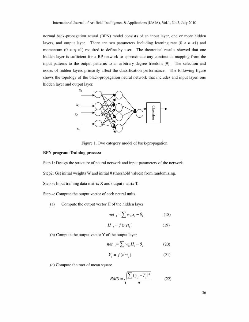
nodes of hidden layers primarily affect the classification performance. The following figure

shows the topology of the black-propagation neural network that includes and input layer, one

hidden layer and output layer.

x1

x2 y

x3

x4

Figure 1. Two category model of back-propagation

BPN program-Training process:

Step 1: Design the structure of neural network and input parameters of the network.

Step2: Get initial weights W and initial θ (threshold values) from randomizing.

Step 3: Input training data matrix X and output matrix T.

Step 4: Compute the output vector of each neural units.

(a) Compute the output vector H of the hidden layer

k ik i knet w x θ= −∑ (18)

( )k kH f net= (19)

(b) Compute the output vector Y of the output layer

j kj i jnet w H θ= −∑ (20)

( )j jY f net= (21)

(c) Compute the root of mean square

2( )j jy TRMS

n

−=∑

(22)

Classifier

器


37

Step 5: Compute the distance δ

(a) Compute the distance δ of the output layer

'( ) ( )j j j jT Y f netδ = − � (23)

(b) Compute the distance δ of the hidden layer

'( ) ( )k j kj j

j

w f netδ δ= ∑ � (24)

Step 6: Compute the modification of W and θ (η is the learning rate, α is the momentum

coefficient)

(a) Compute the modification of W and θ of the output layer

( ) ( 1)kj j k kjw n H w nηδ α∆ = + ∆ − (25)

( ) ( 1)j j jn nθ ηδ α θ∆ = − + ∆ − (26)

(b) Compute the modification of W and θ of the hidden layer

( ) ( 1)ik k i ikw n X w nηδ α∆ = + ∆ − (27)

( ) ( 1)k k kn nθ ηδ α θ∆ = − + ∆ − (28)

Step 7: Renew W and θ

(a) Renew W and θ of the output layer

( ) ( 1)kj kj kjw p w p w= − + ∆ (29)

( ) ( 1)j j jp pθ θ θ= − + ∆ (30)

(b) Renew W and θ of the hidden layer

( ) ( 1)ik ik ikw p w p w= − + ∆ (31)

( ) ( 1)k k kp pθ θ θ= − + ∆ (32)

Step 8: Repeat step 3 to step 7 until converge.

BPN program-testing process:

Step 1: Input the parameters of the network

Step 2: Input the W and θ

Step 3: Input the unknown data matrix X

Step 4: Compute the output vector

(a) Compute the output vector H of the hidden layer

k ik i knet w x θ= −∑ (33)

( )k kH f net= (34)

(b) Compute the output vector Y of the output layer

j kj i jnet w H θ= −∑ (35)


38

( )j jY f net= (36)

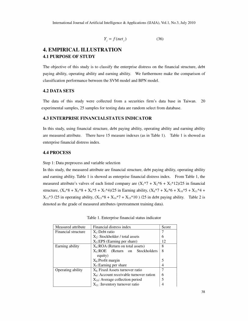
4. EMPIRICAL ILLUSTRATION

4.1 PURPOSE OF STUDY

The objective of this study is to classify the enterprise distress on the financial structure, debt

paying ability, operating ability and earning ability. We furthermore make the comparison of

classification performance between the SVM model and BPN model.

4.2 DATA SETS

The data of this study were collected from a securities firm’s data base in Taiwan. 20

experimental samples, 25 samples for testing data are random select from database.

4.3 ENTERPRISE FINANCIALSTATUS INDICATOR

In this study, using financial structure, debt paying ability, operating ability and earning ability

are measured attribute. There have 15 measure indexes (as in Table 1). Table 1 is showed as

enterprise financial distress index.

4.4 PROCESS

Step 1: Data preprocess and variable selection

In this study, the measured attribute are financial structure, debt paying ability, operating ability

and earning ability. Table 1 is showed as enterprise financial distress index. From Table 1, the

measured attribute’s valves of each listed company are (X1*7 + X2*6 + X3*12)/25 in financial

structure, (X4*8 + X5*8 + X6*5 + X7*4)/25 in Earning ability, (X8*7 + X9*6 + X10*5 + X11*4 +

X12*3 /25 in operating ability, (X13*8 + X14*7 + X15*10 ) /25 in debt paying ability. Table 2 is

denoted as the grade of measured attributes (pretreatment training data).

Table 1. Enterprise financial status indicator

Measured attribute Financial distress index Score

Financial structure X1:Debt ratio 7

X2: Stockholder / total assets 6

X3:EPS (Earning per share) 12

Earning ability X4:ROA (Return on total assets) 8

X5:ROE (Return on Stockholders

equity)

8

X6:Profit margin 5

X7:Earning per share 4

Operating ability X8: Fixed Assets turnover ratio 7

X9: Account receivable turnover ration 6

X10: Average collection period 5

X11 :Inventory turnover ratio 4


39

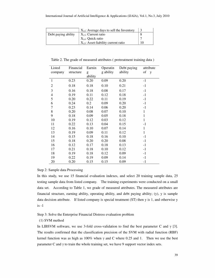
X12: Average days to sell the Inventory 3

Debt paying ability X13: Current ratio 8

X14: Quick ratio 7

X15: Asset-liability current ratio 10

Table 2. The grade of measured attributes ( pretreatment training data )

Listed

company

Financial

structure

Earnin

g

ability

Operatin

g ability

Debt paying

ability

attribute

of y

1 0.23 0.20 0.09 0.20 -1

2 0.18 0.18 0.10 0.21 -1

3 0.16 0.18 0.08 0.17 -1

4 0.19 0.11 0.12 0.18 -1

5 0.20 0.22 0.11 0.19 -1

6 0.24 0.2 0.09 0.20 -1

7 0.23 0.14 0.06 0.20 -1 8 0.20 0.08 0.07 0.10 1

9 0.18 0.09 0.05 0.18 1

10 0.19 0.12 0.03 0.12 1 11 0.22 0.13 0.04 0.15 -1

12 0.16 0.10 0.07 0.14 1

13 0.19 0.09 0.11 0.12 1 14 0.15 0.18 0.16 0.10 -1

15 0.18 0.20 0.20 0.08 -1

16 0.12 0.17 0.18 0.13 -1

17 0.21 0.18 0.10 0.12 -1

18 0.19 0.18 0.12 0.09 -1

19 0.22 0.19 0.09 0.14 -1 20 0.20 0.15 0.15 0.09 -1

Step 2: Sample data Processing

In this study, we use 15 financial evaluation indexes, and select 20 training sample data, 25

testing sample data from listed company. The training experiments were conducted on a small

data set. According to Table 1, we grade of measured attributes. The measured attributes are

financial structure, earning ability, operating ability, and debt paying ability; (y), y is sample

data decision attribute. If listed company is special treatment (ST) then y is 1, and otherwise y

is -1

Step 3: Solve the Enterprise Financial Distress evaluation problem

(1) SVM method

In LIBSVM software, we use 3-fold cross-validation to find the best parameter C and γ [3].

The results confirmed that the classification precision of the SVM with radial function (RBF)

kernel function was as high as 100% when γ and C where 0.25 and 1. Then we use the best

parameter C and γ to train the whole training set, we have 9 support vector index sets.


40

The outputs from LIBSVM software are:

Accuracy = 100% (20/20) (classification)

Mean square error = 0

Squared correlation coefficient = 1 (regression)

Iteration = 108

(2) BPN method

The three parameters of learning rate, momentum and the number of nodes in the hidden layer

should be defined for back-propagation network modeling. In the training model, the four

factors where fed as input nodes. In this network, each unit of the output layer stands for

presence (+1) or absence (-1) of the detected molecule. > 0 as a target value of the presence

and < 0 as a target value of the absence. We adopted the range of 0.6-0.9 and 0.1-0.4 to be the

decisions of learning rate and momentum [17].

In this illustration, there have four measured attributes; we selected four input node, four hidden

nodes, and one output node, that is a good MLP model in this illustration. A very rough

rule-of-thumb for number of hidden nodes defined as h /(5×(m+n)), where h, m, and n represent

the number of training patterns, output nodes and input nodes respectively. Then the

root-mean-square error (RMSE) and classification rate are the measurement indicators to

validate the performance of the training model. Through several trail-and-error experiments,

the structure of 4 -4 -1 model had the best performance.

The outputs from Mathlib software are:

Accuracy = 95% (19/20) (classification)

Iteration = 258

Step 5: Forecast of testing sample data.

We compare the accuracy of different approaches by introducing two error types. TypeＩerror

refer to the situation when matched data is classified as unmatched one, and Type Π error refer

to unmatched data is classified into matched data. The 25 testing sample data from listed

company is denoted as Table 3. The prediction result is listed in Table 4. SVM method

shows the best overall prediction accuracy level at 100 % (see Table 4). Using the unmatched

and unbalanced testing data, MLP method, shows the best overall prediction accuracy level at

96 % (see Table 5).

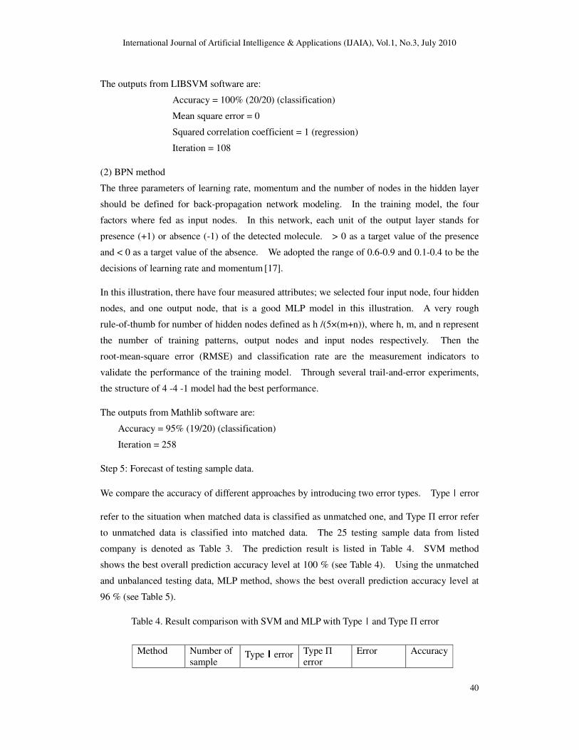
Table 4. Result comparison with SVM and MLP with TypeＩand Type Π error

Method Number of sample

TypeＩerror Type Π error

Error Accuracy


41

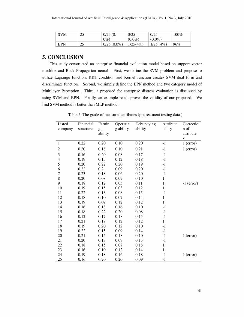
SVM 25 0/25 (0.

0%)

0/25

(0.0%)

0/25

(0.0%)

100%

BPN 25 0/25 (0.0%) 1/25(4%) 1/25 (4%) 96%

5. CONCLUSION

This study constructed an enterprise financial evaluation model based on support vector

machine and Back Propagation neural. First, we define the SVM problem and propose to

utilize Lagrange function, KKT condition and Kernel function creates SVM dual form and

discriminate function. Second, we simply define the BPN method and two category model of

Multilayer Perception. Third, a proposed for enterprise distress evaluation is discussed by

using SVM and BPN. Finally, an example result proves the validity of our proposed. We

find SVM method is better than MLP method.

Table 5. The grade of measured attributes (pretreatment testing data )

Listed company

Financial structure

Earning

ability

Operating ability

Debt paying ability

Attribute of y

Correction of

attribute

y

1 0.22 0.20 0.10 0.20 -1 1 (error)

2 0.20 0.18 0.10 0.21 -1 1 (error)

3 0.16 0.20 0.08 0.17 -1 4 0.19 0.15 0.12 0.18 -1

5 0.20 0.22 0.20 0.19 -1

6 0.22 0.2 0.09 0.20 -1 7 0.23 0.18 0.06 0.20 -1

8 0.20 0.08 0.09 0.10 1

9 0.18 0.12 0.05 0.11 1 -1 (error)

10 0.19 0.15 0.03 0.12 1

11 0.22 0.13 0.08 0.15 -1

12 0.18 0.10 0.07 0.14 1 13 0.19 0.09 0.12 0.12 1

14 0.16 0.18 0.16 0.10 -1

15 0.18 0.22 0.20 0.08 -1 16 0.12 0.17 0.18 0.15 -1

17 0.21 0.18 0.12 0.12 1

18 0.19 0.20 0.12 0.10 -1

19 0.22 0.15 0.09 0.14 -1

20 0.21 0.15 0.18 0.10 -1 1 (error)

21 0.20 0.13 0.09 0.15 -1

22 0.18 0.15 0.07 0.18 1

23 0.16 0.10 0.12 0.14 1

24 0.19 0.18 0.16 0.18 -1 1 (error)

25 0.16 0.20 0.20 0.09 -1


42

ACKNOWLEDGEMENTS

I would like to thank the anonymous reviewers for their constructive comments on this

paper.

REFERENCES [1 ] Bongini, P., Laeven, L., and Majnoni, G., (2002), “How good is the market at assessing bank

fragility? A Horse Race between different indictors”, Journal of banking & Finance, Vol. 26, pp.

1011-1028.

[2 ] Chakraborty, S., Sharma, S. K., (2007), “Prediction of corporate financial health by Artificial

Neural Network”, International Journal of Electronic Finance, Vol. 1, No. 4, pp. 442-459

[3 ] Chang, C. C., and Lin, C. J., (2009), LIBSVM: a library for support vector machines. Software

available at http://www.csie.ntu.edu.tw/”cjin/libsvm. (2009-11-18)

[4 ] Chen, A. S. and Leung, M. T., (2004), “Regression Neural Network for error correction in foreign

exchange forecasting and trading”, Computers & Operations Research, Vol. 31, pp. 1049-1068.

[5 ] Chen, A. S., Leung , M. T. and Daouke, H.,(2003), “Application of neural networks to an

emerging financial market: Foresting and training the Taiwan stock index”, Computers and

Operations Research, Vol. 31, pp. 901-923.

[6 ] Coats, P. K. and Fant, L. F., “Recognizing financial distress pattern using a neural network tool,

Financial”, Management, Autumn, (1993) pp. 142-155

[7 ] Cristianini, N.,and Shawe-Taylor, J., (2000), “An Introduction to Support Vector Machines”,

Cambridge University Press.

[8 ] Fan, A., and Palaniswami, M., (2000), “Selecting bankruptcy predictors using a support vector

machine approach”, Proceedings of the International Joint Conference on Neural Network, pp.

340-352.

[9 ] Fausett, L., (1994), “Fundamentals of Neural Networks: Architecture”, Algorithms and Applications,

New Jersely: Prentice-Hall.

[10 ] Gestel, T. V., Baestens, B., Suykens, J., and Poel, D. V., (2006), “Bayesian kernel based on

classification for financial distress detection”, European Journal of operational Research, Vol. 172,

pp. 979-1003.

[11 ] Keerthi, S. S. and Lin, C. C., (2003), “Asymptotic behaviors of Support vector machines with

Gaussian Kernel”, Neural Computation, Vol. 15, No. 7, pp. 1667-1689.

[12 ] O’Neill, T. J. and Penm, J., (2007),” A new approach to testing credit rating of financial debt

issuers”, International Journal of Services and Standards, Vol.3, No.4, 390-401

[13 ] Odom, M., and Sharda, R., (1990), “A neural network model for bankruptcy prediction”, IEEE

INNS International Joint Conference on Neural Networks, Vol. 12, pp. 163-168.

[14 ] Pompe, P. M. and Bilderbeek, J., (2005), “The Prediction of Bankruptcy of Small and Medium

Size Industrial Firms”, Journal of Business Venturing, Vol. 20, pp. 847-868.

[15 ] Randall, S. S. and Dorsey, R. E (2000), " Dorsey, Reliable Classification Using Neural Networks:

A Genetic Algorithm and Back Propagation Comparison”, Decision Support Systems, 30, pp.

11-22.

[16 ] Schölkopf, S. C. Burges, J. C., and Smola, A. J., (1999), “Advances in Kernel Methods: Support

Vector Learning”, MIT Press, Cambridge, MA.


43

[17 ] Su, C. T., Yang, T. , and Ke, C. M. , (2002), “A neural network approach for semiconductor wafer

post-sawing inspection”, IEE Transaction on Semiconductor Manufacturing,, Vol. 15, No. 2, pp.

260-266.

[18 ] Tam, K. Y. and Kiang, M., (1992), “ Managerial applications of neural network: the case of bank

failure predictions”, Management Sciences, Vol. 38, pp. 927-947

[19 ] Vapnik, V. N., (1999), “Statistical learning theory”, New York: J. Wiley- Interscience.

[20 ] enugopal, V. V. and Baets, W., (1994), “Neural Networks and Statistical Techniques in Marketing

Research: A Concept Comparison”, Marketing Intelligence and Planning , Vol.1, No. 7, pp.

23-30

[21 ] Yuan, S. F. and Chu, F. L., (2006), “Support vector machines based on fault diagnosis for

turbo-pump rotor”, Machine Systems and Signal Processing, Vol. 20, pp. 939-952

[22 ] Yuan, X., (2007), “Grey Relational Evaluation of Financial Situation of Listed Company”, Journal

of Modem Accounting and Auditing, Vol. 3, No. 3, pp. 41-44

[23 ] Zhang, Z., Hu, M., and Platt, H., (1999), “Artificial neural networks in bankruptcy prediction:

General framework and cross-validation analysis”, European Journal of Operation Research, Vol.

116 pp. 16-32.

[24 ] Singh, A. P., Rai, C. S., and Chandra, P., (2010), “Empirical Study of FFANN Tolerance to Weight

Stuck at Max/Min Fault, International Journal of Artificial Intelligence & Application, Vol. 1, No. 2,

pp. 13-21

Ming-Chang Lee is Assistant Professor of

Department of Information Management at

Fooyin University and National Kaohsiung

University of Applied Sciences. His qualifications

include a Master degree in applied Mathematics

from National Tsing Hua University and a PhD

degree in Industrial Management from Nation

Cheng Kung University. His research interests

include knowledge management, parallel

computing, and data analysis. His publications

include articles in the journal of Computer &

Mathematics with Applications, International

Journal of Operation Research, Computers &

Engineering, American Journal of Applied

Science and Computers, Industrial Engineering,

International Journal innovation and Learning, Int.

J. Services and Standards, Lecture Notes in

computer Science (LNCS), International Journal

of Computer Science and Network Security,

Journal of Convergence Information Technology

and International Journal of Advancements in

computing Technology.

To Chang is an Assistant Professor and the

Chairman of Department of Information

Management at Shu-Te University, Taiwan. His

qualifications include Master degree in Computer

Science from Naval Postgraduate School, USA

and PhD degree in Electronic Engineering from

Chung Cheng Institute of Technology, Taiwan.

His research interests include Information

Security, Management Information Systems, and

Enterprise Resource Planning. His publications

include articles in International Journal

Innovation and Learning, Int. J. Services and

Standards, and International Journal of Computer

Science and Network Security.

Documents

Comparison of Support Vector Machine and Back ...aircconline.com/ijaia/V1N3/0710ijaia3.pdfComparison of Support Vector Machine and Back Propagation Neural Network in Evaluating the