The Black-Scholes-Merton

Model

Options, Futures, and Other Derivatives, 8th Edition, Copyright © John C. Hull 2012

The Black-Scholes-Merton model is one of the most

important concepts in modern financial theory.

It was developed in 1973 by Fisher Black, Robert

Merton and Myron Scholes and is still widely used

today, and regarded as one of the best ways of

determining fair prices of options.

It is a model of price variation over time of financial

instruments such as stocks that can, among other

things, be used to determine the price of a European

option.

2

The Black-Scholes-Merton model

The Black-Scholes-Merton differential equation is an

equation that must be satisfied by the price of any

derivative dependent on a non-dividend-paying stock.

It is derived by setting up a riskless portfolio

consisting of a position in the derivative and a

position in the stock.

In the absence of arbitrage opportunities, the return

from the portfolio must be given by the risk-free

interest rate.

3

The Black-Scholes-Merton model

The reason a riskless portfolio can be set up is that

the stock price and the derivative price are both

affected by the same underlying source of

uncertainty: the stock price movements.

In any short period of time, the price of the derivative

is perfectly correlated with the price of the underlying

stock.

When an appropriate portfolio of the stock and the

derivative is established, the gain or loss from the

stock position always offsets the gain or loss from the

derivative position so that the overall value of the

portfolio at the end of the short period of time is

known with certainty.

4

The Black-Scholes-Merton model

Suppose, for example, that at a particular point in time the

relationship between a small change ΔS in the stock price

and the resultant small change Δc in the price of a call

option is given by:

Δc = 0.4ΔS

The riskless portfolio would consist of :

a) A long position in 0.4 shares.

b) A short position in one call option.

Suppose, e.g., that the stock price increases by 10 cents.

The option price will increase by 4 cents and the 0.4 x 10

= 4 cents gain on the shares is equal to the 4 cents loss

on the short option position.

5

The Black-Scholes-Merton model

In Black-Scholes-Merton analysis, the position in the stock

and the derivative is riskless for only a very short period of

time.

To remain riskless, it must be adjusted, or rebalanced,

frequently.

For example, the relationship between ΔS and Δc might

change from Δc = 0.4ΔS today to Δc = 0.5ΔS in 2 weeks.

This would mean that, in order to maintain the riskless

position, an extra 0.1 share would have to be purchased for

each call option sold.

It is true that the return from the riskless portfolio in any

very short period of time must be the risk-free interest rate.

6

The Black-Scholes-Merton model

The assumptions we use to derive the Black-Scholes-Merton

differential equation are:

a) Changes in the stock price in a short period of time are

normally distributed.

b) The short selling of securities with full use of proceeds is

permitted.

c) There are no transactions costs or taxes; all securities are

perfectly divisible.

d) There are no dividends during the life of the derivative.

e) There are no riskless arbitrage opportunities.

f) Security trading is continuous.

g) The risk-free rate of interest is constant and the same for

all maturities.

7

Black-Scholes-Merton equation: Assumptions

Normal Distribution of Stock Prices

The model of stock price behaviour used by Black,

Scholes, and Merton assumes that % changes in the

stock price in a short period of time are normally

distributed.

Consider a stock whose price is S, m is expected return

on the stock, and s is the volatility of the stock price.

In a short period of time of length Dt, the return on the

stock is normally distributed:

where ΔS is the change in the stock price S in time Δt,

and φ(m, v) denotes a normal distribution with mean m

and variance v.

ttS

SDD

D 2,sm

8

It follows from this assumption that lnST is normal, so that ST is lognormally distributed:

where ST is the stock price at a future time T and S0 is the stock price at time 0.

9

,2

lnln

or

,2

lnln

22

0

22

0

TTSS

TTSS

T

T

ss

m

ss

m

Normal Distribution of Stock Prices

10

A variable that has a lognormal distribution can take any

value between zero and infinity.

The figure below illustrates the shape of a lognormal

distribution.

Unlike the normal distribution, it is skewed so that the

mean, median, and mode are all different.

The Lognormal Distribution

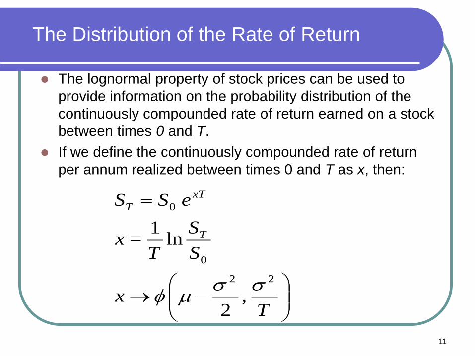
The lognormal property of stock prices can be used to

provide information on the probability distribution of the

continuously compounded rate of return earned on a stock

between times 0 and T.

If we define the continuously compounded rate of return

per annum realized between times 0 and T as x, then:

11

,2

ln1

=

22

0

0

Tx

S

S

Tx

eSS

T

xT

T

ssm

The Distribution of the Rate of Return

Thus, the continuously compounded rate of return

per annum is normally distributed.

As T increases, the standard deviation of x declines.

To understand the reason for this, consider two

cases: T = 1 and T = 20.

This implies that we are more certain about the

average return per year over 20 years than we are

about the return in any one year.

12

The Distribution of the Rate of Return

The Black-Scholes Differential Equation

13

2

222 rƒ

S

ƒS½ σ

S

ƒrS

t

ƒ

The Black-Scholes-Merton differential equation is:

where:

f is the price of a call option or other derivative contingent on S

f is a variable of S and t

S is the price of the underlying stock

r is the risk-free interest rate

14

The Black-Scholes-Merton equation has many solutions,

corresponding to all the different derivatives that can

be defined with S as the underlying variable.

The most famous solutions are those based on the

prices of European call and put options.

A European option may be exercised only at the

expiration date of the option, i.e. at a single pre-

defined point in time.

An American option on the other hand may be

exercised at any time before the expiration date.

The Black-Scholes Differential Equation

15

TdT

TrKSd

T

TrKSd

dNSdNeKp

dNeKdNSc

rT

rT

ss

s

s

s

1

0

2

0

1

102

210

)2/2()/ln(

)2/2()/ln( where

)( )(

)( )(

These formulas are:

The Black-Scholes Differential Equation

The variables c and p are the European call and

European put price

S0 is the stock price at time zero

K is the strike price

r is the continuously compounded risk-free rate

σ is the stock price volatility

T is the time to maturity of the option.

16

The Black-Scholes Differential Equation

N(x) is the probability that a normally distributed variable

with a mean of zero and a standard deviation of 1 is

less than x

17

The Black-Scholes Differential Equation

The one parameter in the Black-Scholes-Merton

pricing formulas that cannot be directly observed is

the volatility of the stock price.

This can be estimated from a history of the stock

price.

In practice, traders usually work with what are known

as implied volatilities.

These are the volatilities implied by option prices

observed in the market.

18

Implied Volatility

Nature of Volatility

Volatility is usually much greater when the market is

open (i.e. the asset is trading) than when it is closed.

For this reason time is usually measured in “trading

days” not calendar days when options are valued.

It is assumed that there are 252 trading days in one

year for most assets.

Suppose it is April 1 and an option lasts to April 30 so

that the number of days remaining is 30 calendar days

or 22 trading days.

The time to maturity would be assumed to be 22/252

= 0.0873 years.

19

Dividends

Up to now, we have assumed that the stock on which

the option is written pays no dividends.

The Black-Scholes-Merton model can be modified to

take account of dividends.

As known, European options can be analysed by

assuming that the stock price is the sum of two

components:

a) a riskless component that corresponds to the

known dividends during the life of the option and

b) a risky component.

20

Dividends

The riskless component, at any given time, is the

present value of all the dividends during the life of the

option discounted from the ex-dividend dates to the

present at the risk-free rate.

By the time the option matures, the dividends will have

been paid and the riskless component will no longer

exist.

Hence, the Black-Scholes-Merton formulae can be

used provided that the stock price is reduced by the

present value of all the dividends during the life of the

option, the discounting being done from the ex-

dividend dates at the risk-free rate.

21