A Lie Symmetry Analysis of the Black-Scholes Merton

A Lie Symmetry Analysis of the

Black-Scholes Merton Finance Model

through modified Local one-parameter

transformations

by

Tshidiso Phanuel Masebe

Submitted in accordance with the requirements for the degree of

Doctor of Philosophy in the subject Applied Mathematics at

the University of South Africa

September 2014

Supervisor : Dr J.M. Manale

Contents

Introduction 1

1 Local One-parameter Point Symmetries 4

1.1 Local One-parameter Point transformations . . . . . . . . . . . . . . 4

1.2 Local One-parameter Point transformation groups . . . . . . . . . . . 5

1.3 The group generator . . . . . . . . . . . . . . . . . . . . . . . . . . . 7

1.4 Prolongations formulas . . . . . . . . . . . . . . . . . . . . . . . . . 7

1.4.1 The case N = 2, with x1 = x and x2 = y . . . . . . . . . . . . 8

1.4.2 Invariant functions in R2 . . . . . . . . . . . . . . . . . . . . . 10

1.4.3 Multi-dimensional cases . . . . . . . . . . . . . . . . . . . . . 11

1.4.4 Invariant functions in RN . . . . . . . . . . . . . . . . . . . . 13

1.5 Determining equations . . . . . . . . . . . . . . . . . . . . . . . . . . 14

1.6 Lie algebras . . . . . . . . . . . . . . . . . . . . . . . . . . . . . . . . 14

1.7 Solvable Lie algebras . . . . . . . . . . . . . . . . . . . . . . . . . . . 15

1.8 Lie equations . . . . . . . . . . . . . . . . . . . . . . . . . . . . . . . 16

1.9 Canonical Parameter . . . . . . . . . . . . . . . . . . . . . . . . . . . 17

1.10 Canonical variables . . . . . . . . . . . . . . . . . . . . . . . . . . . . 17

1.11 One Dependent and Two Independent Variables. . . . . . . . . . . . 21

i

1.12 One Dependent and Three Independent Variables. . . . . . . . . . . . 22

1.13 One Dependent and Four Independent Variables. . . . . . . . . . . . 25

1.14 One Dependent and n Independent Variables. . . . . . . . . . . . . . 26

1.15 m Dependent and n Independent Variables. . . . . . . . . . . . . . . 27

2 Symmetry Analysis of Black-Scholes Equation 30

2.1 Symmetries . . . . . . . . . . . . . . . . . . . . . . . . . . . . . . . . 30

2.1.1 Finite symmetry transformations . . . . . . . . . . . . . . . . 32

2.2 Transformation to heat equation . . . . . . . . . . . . . . . . . . . . . 33

2.3 Invariant Solutions . . . . . . . . . . . . . . . . . . . . . . . . . . . . 35

3 Introduction of new method 37

3.1 The transformed one-dimensional Black-Scholes equation . . . . . . . 37

3.2 Solution of determining equation for (3.6) . . . . . . . . . . . . . . . 39

3.2.1 Infinitesimals for equation (3.6) . . . . . . . . . . . . . . . . . 44

3.2.2 The symmetries for equation (3.6) . . . . . . . . . . . . . . . . 45

3.2.3 Table of Commutators . . . . . . . . . . . . . . . . . . . . . . 46

3.3 Invariant Solution for equation (3.6) . . . . . . . . . . . . . . . . . . . 47

3.3.1 Solutions for equation 3.97 . . . . . . . . . . . . . . . . . . . . 51

3.4 Two-Dimensional Black-Scholes Equation . . . . . . . . . . . . . . . . 54

3.4.1 Transformed two-dimensional Black-Scholes Equation . . . . . 54

3.4.2 Solution for determining equation for (3.109) . . . . . . . . . . 55

3.4.3 Infinitesimals for equation (3.109) . . . . . . . . . . . . . . . . 63

3.4.4 Symmetries for equation (3.109) . . . . . . . . . . . . . . . . . 66

3.4.5 Invariant Solution for equation (3.109) . . . . . . . . . . . . . 70

ii

4 Transformation of equation (3.6) to heat equation 74

4.1 Transformation . . . . . . . . . . . . . . . . . . . . . . . . . . . . . . 75

5 Further Applications 80

5.1 Gaussian type partial differential equation . . . . . . . . . . . . . . . 80

5.1.1 Solution of determining equation . . . . . . . . . . . . . . . . 81

5.1.2 Infinitesimals . . . . . . . . . . . . . . . . . . . . . . . . . . . 84

5.1.3 Symmetries . . . . . . . . . . . . . . . . . . . . . . . . . . . . 84

5.1.4 Invariant Solutions . . . . . . . . . . . . . . . . . . . . . . . . 85

5.2 Symmetries in the epidemiology of HIV and AIDS . . . . . . . . . . . 89

5.3 Integrating (5.75) . . . . . . . . . . . . . . . . . . . . . . . . . . . . . 91

5.3.1 Applying the Lie symmetry generator to (5.78) . . . . . . . . 91

5.3.2 Infinitesimals . . . . . . . . . . . . . . . . . . . . . . . . . . . 95

5.3.3 The symmetries . . . . . . . . . . . . . . . . . . . . . . . . . . 95

5.3.4 Construction of invariant solutions . . . . . . . . . . . . . . . 96

Conclusion 100

Appendices i

Appendix A: Manale’s formulas and the infinitesimal ω . . . . . . . . . . . i

Appendix B: Useful limit results . . . . . . . . . . . . . . . . . . . . . . . . v

Appendix C: Solution for determining equation (2.5) . . . . . . . . . . . . vii

iii

List of Figures

3.1 Commutator Table . . . . . . . . . . . . . . . . . . . . . . . . . . . . 47

3.2 Plot for the solution (3.100) with dependent variable u represented

on the vertical axis and independent variable t represented on the

horizontal axis . . . . . . . . . . . . . . . . . . . . . . . . . . . . . . 51

3.3 Plot for solution (3.102) with dependent variable u represented on the

vertical axis and independent variable λ represented on the horizontal

axis . . . . . . . . . . . . . . . . . . . . . . . . . . . . . . . . . . . . 52

3.4 Plot for solution (3.107) with dependent variable u represented on the

vertical axis and independent variable r represented on the horizontal

axis . . . . . . . . . . . . . . . . . . . . . . . . . . . . . . . . . . . . 54

3.5 Plot for solution (3.226)with dependent variable u represented on the

vertical axis and independent variable r represented on the horizontal

axis . . . . . . . . . . . . . . . . . . . . . . . . . . . . . . . . . . . . 73

iv

Abstract

The thesis presents a new method of Symmetry Analysis of the Black-Scholes Merton

Finance Model through modified Local one-parameter transformations. We deter-

mine the symmetries of both the one-dimensional and two-dimensional Black-Scholes

equations through a method that involves the limit of infinitesimal ω as it approaches

zero. The method is dealt with extensively in [23]. We further determine an invariant

solution using one of the symmetries in each case. We determine the transformation

of the Black-Scholes equation to heat equation through Lie equivalence transforma-

tions.

Further applications where the method is successfully applied include working out

symmetries of both a Gaussian type partial differential equation and that of a differ-

ential equation model of epidemiology of HIV and AIDS. We use the new method to

determine the symmetries and calculate invariant solutions for operators providing

them.

Keywords: Black-Scholes equation; Partial differential equation; Lie Point Symme-

try; Lie equivalence transformation; Invariant solution.

v

Declaration

Student number: 46640193

I declare that A Lie Symmetry Analysis of the Black-Scholes Merton Fi-

nance Model through modified Local one-parameter transformations is my

own work and that all the sources that I have used or quoted have been indicated

and acknowledged by means of a complete list of references.

SIGNATURE DATE

vi

Dedication

I would like to dedicate this thesis to my father Philip Masebe, my late mother, Dolly

Daisy Masebe who has always been my pillar of strength and an encouragement me

to work hard in my studies. I further would like to thank my son, Reotshepile Phillip

Masebe who has always been a source of inspiration and motivation for me to hold

steadfast.

vii

Acknowledgement

• I am indebted to my supervisor, Dr J.M. Manale for the guidance, patience

and professional assistance he has offered throughout this thesis. It is with

gratitude that I have tapped from his vast wisdom and knowledge.

• Special words of thank you go to Prof M. T. Kambule for having introduced

me to Symmetry Analysis. I also acknowledge the teaching I received from

Prof N.H. Ibragimov in my Masters degree programme. It has rounded my

understanding of Lie Symmetry Analysis. I also thank Dr M.P. Mulaudzi for

the lessons he offered me on Mathematics of Finance.

• Words of thank you go to all my friends, former colleagues and current col-

leagues at Tshwane University of Technology , and to Staff members in the

Mathematics Department at University of South Africa. Family members,

brothers and a sister with whom we have a formidable bond I say thanks.

Thanks to a special lady for her words of encouragement, and expressing con-

fidence in my ability to put together an undertaking of this nature.

• I acknowledge the financial support of my institution Tshwane University of

Technology and the financial aid at University of South Africa.

• With God everything is possible.

viii

Introduction

The Lie group analysis of differential equations is the area of mathematics pioneered

by Sophus Lie in the 19th century (1849-1899). Sophus Lie made a profound and

far-reaching discovery that all ad-hoc techniques designed to solve ordinary differen-

tial equations (e.g separable variables, homogeneous, exact) could be explained and

deduced simply by his theory. These techniques were in fact special cases of a general

integration procedure of classifying ordinary differential equations in terms of their

symmetry groups. This discovery led to Lie identifying a full set of equations which

could be integrated or reduced to lower order equations by his method [6],[14].

The Lie Symmetry method is analytic and highly algorithmic. The method system-

atically unifies and extends ad-hoc techniques to construct explicit solutions for dif-

ferential equations. The emphasis is on explicit computational algorithms to discover

symmetries admitted by differential equations and to construct invariant solutions

resulting from the symmetries [6],[13].

Lie group analysis established itself to be an effective method of solving non-linear

differential equations analytically. In fact the first general solution of the problem

of classification was given by Sophus Lie for an extensive class of partial differential

equations [14]. Since then many researchers have done work on various families of

differential equations. The results of their work have been captured in several out-

standing literary works by amongst others Ibragimov (1999), Hydon(2000), Bluman

and Anco(2002), etc [6], [9], [13].

1

The present project titled A Lie Symmetry Analysis of the Black-Scholes

Merton Finance Model through modified Local one-parameter transfor-

mations seeks to explore the analysis of the widely used one-dimensional model of

Black-Scholes partial differential equation through determining the new symmetries

and invariant solutions of some of these symmetries. The analysis is through a new

method developed in [23], [28]. Further exploration of the method can be found in

[25], [26],[27]. Throughout the project we use Lie point symmetries.

The Black-Scholes equation is a partial differential equation that governs the value

of financial derivatives. Determining the value of derivatives had been a problem in

finance for almost 70 years since 1900. In the early 70s, Black and Scholes made

a pioneering contribution to finance by developing a Black-Scholes equation under

restrictive assumptions and the option valuation formula. Scholes obtained a No-

bel Prize for economics in 1997 for his contribution (Black had passed on in 1995

and could not receive the prize personally) [32]. Furthermore, information on the

derivation of and the restrictive assumptions in the development of the Black-Scholes

equation can be obtained in the texts [4], [8], [10], [11], [12], [21], [22] and [30].

The thesis outline is as follows:

Chapter 1 presents the concept of Local One-parameter Point Symmetries. We

introduce concepts of Local One-parameter Point transformations, generator, pro-

longation formulas, determining equation and Lie algebras. These concepts serve as

tools in the analysis of the Black-Scholes partial differential equation.

Chapter 2 presents the Symmetry Analysis of equation (2.1) as outlined in [9]. The

chapter presents the symmetry of (2.1),finite symmetry transformations and the

transformation of the equation (2.1) to the heat equation.

2

Chapter 3 is the core of the thesis. It introduces the Symmetry Analysis of equation

(2.1) by using the method developed through contributions in ([23]) and ([28]). The

chapter details the symmetries of one-dimensional Black-Scholes equation (2.1) as

well as the two-dimensional case through modified Local one-parameter transforma-

tions.

Chapter 4 involves the transformation of the transformed Black-Scholes equation to

heat through Lie equivalence transformations. We calculate this transformation by

using a method similar but with slight modification to that developed in [17].

Chapter 5 presents other areas where the method was successfully applied. The appli-

cation includes determining the symmetries and invariant solutions of the Gaussian

type differential equation and symmetries in the epidemiology of HIV and AIDS.

Contributions to the study

The thesis is based on peer reviewed contributions to the study as outlined in the

publications ([1]) and ([28]). Several texts for example ([6]), ([13]),([14]) etc. present

symmetries of differential equations in the way initially introduced by Sophus Lie.

However, in this publications we introduce an alternative way to determine these

symmetries, and the method present new additional symmetries.

3

Chapter 1

Local One-parameter Point

Symmetries

The chapter presents the underlying theory of Lie Symmetry Analysis and the tools

we will use in subsequent chapters. The most common of all symmetries in practice

are Local One-parameter Point symmetries.

1.1 Local One-parameter Point transformations

To begin, we consider the following definition.

Definition 1 Let

x = G (x; ε) (1.1)

be a family of one-parameter ε ∈ R invertible transformations, of points x =

(x1, · · · , xN) ∈ RN into points x = (x1, · · · , xN) ∈ RN. These are known as one-

parameter transformations, and subject to the conditions

x|ε=0 = x. (1.2)

That is,

G (x; ε)

∣∣∣∣ε=0

= x. (1.3)

4

Expanding (1.1) about ε = 0, in some neighborhood of ε = 0, we get

x = x + ε

(∂G

∂ε

∣∣∣∣∣ε=0

)+ε2

2

(∂2G

∂ε2

∣∣∣∣∣ε=0

)+ · · · = x + ε

(∂G

∂ε

∣∣∣∣∣ε=0

)+O

(ε2). (1.4)

Letting

ξ (x) =∂G

∂ε

∣∣∣∣∣ε=0

, (1.5)

reduces the expansion to

x = x + εξ (x) +O(ε2). (1.6)

Definition 2 The expression

x = x + εξ (x) , (1.7)

is called a Local One-parameter Point transformation.

The components of ξ (x) are called the infinitesimals of (1.1) [6].

1.2 Local One-parameter Point transformation groups

The set G of transformations

xεi = x + εi

(∂G

∂εi

∣∣∣∣∣εi=0

)+ε2i2

(∂2G

∂ε2i

∣∣∣∣∣εi=0

)+ · · · , i = 1, 2, 3, · · · , (1.8)

becomes a group only when truncated at O (ε2).

That is, G is a group since the following properties hold under binary operation +:

1. Closure. If xε1 , xε2 ∈ G and ε1, ε2 ∈ R, then

xε1 + xε2 = (ε1 + ε2)ξ (x) = xε3 ∈ G, and ε3 = ε1 + ε2 ∈ R.

2. Identity. If x0 ≡ I ∈ G such that for any ε ∈ R

x0 + xε = xε = xε + x0,

then x0 is an identity in G.

5

3. Inverses. For xε ∈ G, ε ∈ R, there exists x−1ε ∈ G, such that

x−1ε + xε = xε + x−1

ε , x−1ε = xε−1 ,

and ε−1 = −ε ∈ D, where + is a binary composition of transformations and it is

understood that xε = xε − x. Associativity follows from the closure property.

Example 1 :

Group of Rotations in the Plane

x1 = x1 cos ε+ x2 sin ε,

x2 = x2 cos ε− x1 sin ε.

That is,

x1 = x1 + x2ε,

x2 = x2 − x1ε.

Example 2 : Group of Translations in the Plane

xi = xi + ε,

xj = xj.

Example 3 :

Group of Scalings in the Plane

6

xi = (1 + ε)xi,

xj = (1 + ε)2xj. [6], [15].

1.3 The group generator

The Local One-parameter Point transformations in (1.7) can be rewritten

in the form

x = x + εξ (x) · ∇ x, (1.9)

so that

x = (1 + εξ (x) · ∇) x. (1.10)

An operator,

G = ξ (x) · ∇, (1.11)

can then be introduced, so that (1.9) assumes the form

x = (1 + εG) x. (1.12)

The operator (1.11) has the expanded form

G =N∑k=1

ξk∂

∂xk, (1.13)

or simply

G = ξk∂

∂xk. [6], [16], [18]. (1.14)

1.4 Prolongations formulas

It often happens that the invariant function F does not only depend on the point x

alone, but also on the derivatives. When that is the case then we have to use the

prolonged form of the operator G.

7

1.4.1 The case N = 2, with x1 = x and x2 = y

The case N = 2, with x1 = x and x2 = y reduces (1.13) to

G = ξ(x, y)∂

∂x+ η(x, y)

∂

∂y. (1.15)

In determining the prolongations, it is convenient to use the operator

of total differentiation

D =∂

∂x+ y′

∂

∂y+ y′′

∂

∂y′+ · · · , (1.16)

where

y′ =dy

dx, y′′ =

d2y

dx2, · · · . (1.17)

The derivatives of the transformed point is then

y′ =dy

dx. (1.18)

Since

x = x+ εξ and y = y + εη, (1.19)

then

y′ =dy + εdη

dx+ εdξ. (1.20)

That is,

y′ =dy/dx+ εdη/dx

dx/dx+ εdξ/dx. (1.21)

Now introducing the operator D:

y′ =y′ + εD(η)

1 + εD(ξ)=

(y′ + εD(η))(1− εD(ξ))

1− ε2(D(ξ))2. (1.22)

Hence

8

y′ =y′ − ε(D(η)− y′D(ξ))− ε2(D(ξ))

1− ε2(D(ξ))2. (1.23)

That is,

y′ = y′ + ε(D(η)− y′D(ξ)), (1.24)

or

y′ = y′ + εζ1, (1.25)

with

ζ1 = D(η)− y′D(ξ). (1.26)

It expands into

ζ1 = ηx + (ηy − ξx)y′ − y′2ξy. (1.27)

The first prolongation of G is then

G[1] = ξ(x, y)∂

∂x+ η(x, y)

∂

∂y+ ζ1 ∂

∂y′. (1.28)

For the second prolongation, we have

y′′ =y′′ + εD(ζ1)

1 + εD(ξ)≈ y′′ + εζ2, (1.29)

with

ζ2 = D(ζ1)− y′′D(ξ). (1.30)

This expands into

ζ2 = ηxx + (2ηxy − ξxx)y′ + (ηyy − 2ξxy)y′2

− y′3ξyy + (ηy − 2ξx − 3y′ξy)y′′. (1.31)

The second prolongation of G is then

9

G[2] = ξ(x, y)∂

∂x+ η(x, y)

∂

∂y+ ζ1 ∂

∂y′+ ζ2 ∂

∂y′′. (1.32)

Most applications involve up to second order derivatives. It is reasonable then to

pause here, for this case [14] .

1.4.2 Invariant functions in R2

Theorem 1 A function F (x, y) is an invariant of the group of transformations (1.13)

if for each point (x, y) it is constant along the trajectory determined by the totality

of transformed points (x, y):

F (x, y) = F (x, y). (1.33)

This requires that

GF = 0, (1.34)

leading to the characteristic system

dx

ξ=dy

η. (1.35)

Proof. Consider the Taylor series expansion of F (x) with respect to ε:

F (x, y) = F (x, y)

∣∣∣∣ε=0

+ ε∂F

∂ε

∣∣∣∣∣ε=0

+ · · · . (1.36)

This can be written in the form

F (x, y) = F (x, y)

∣∣∣∣ε=0

+ ε

(∂x

∂ε

∂F

∂x+∂∂y

∂ε

∂F

y

) ∣∣∣∣∣ε=0

+ · · · . (1.37)

That is,

F (x, y) = F (x, y) + ε

(ξ∂F

∂x+ η

∂F

y

) ∣∣∣∣∣ε=0

+ · · · , (1.38)

or

F (x, y) = F (x, y) + ε

(ξ∂

∂x+ η

∂

∂y

)F + · · · . (1.39)

Hence

F (x, y) = F (x, y) + εGF , (1.40)

10

with

G = ξ∂

∂x+ η

∂

∂y. (1.41)

For ε = 0 then we get

F (x, y) = F (x, y), (1.42)

thus proving the theorem [16].

1.4.3 Multi-dimensional cases

In dealing with the multi-dimensional cases, we may recast the generator (1.13) as

G = ξi∂

∂xi+ ηα

∂

∂uα. (1.43)

We consider the kth-order partial differential equation

F (x, u, u(1), u(2), ..., u(k)) where x = (x1 . . . xn), u(1) =∂u

∂x. (1.44)

By definition of symmetry, the transformations (1.1) form a symmetry group G of the

system (1.44) if the function u = u(x) satisfies (1.43) whenever the function u = u(x)

satisfies (1.44). The transformed derivatives u(1), . . . , u(k) are found from (1.4) by

using the formulae of change of variables in the derivatives, Di = Di(fj)Dj. [6]

Here

Di =∂

∂xi+ uai (

∂

∂ua) + uaij(

∂

∂uaj+ · · · ) (1.45)

is the total derivative operator w.r.t. xi and Dj is given in terms of the transformed

variables. The transformations (1.13) together with the transformations on u(1) form

a group, G[1], which is the first prolonged group which acts in the space (x, u, u(1)).

Likewise, we obtain the prolonged groups G[2] and so on up to G[k].

The infinitesimal transformations of the prolonged groups are:

uai ≈ uai + aζai (x, u, u(1)) ,

uaij ≈ uaij + aζaij(x, u, u(1), u(2)) ,

...

uai1...ik ≈ uai1...ik + aζai1...ik(x, u, u(1), . . . , u(k)) .

(1.46)

11

The functions ζai (x, u, u(1)), ζaij(x, u, u(1), u(2)) and

ζai1...ik(x, u, u(1), . . . , u(k)) are given, recursively, by the prolongation formulas :

ζai = Di(ηa)− uajDi(ξ

j) ,

ζaij = Dj(ζai )− uilDj(ξ

l) ,

... (1.47)

ζai1...ik = Dik(ζai1...ik−1

)− uli1...ik−1Dik(ξ

l) .

The generator of the prolonged groups are:

G[1] = ξi(x, u) ∂∂xi

+ ηa(x, u) ∂∂ua

+ ζai (x, u, u(1))∂∂uai

,

... (1.48)

G[k] = ξi(x, u) ∂∂xi

+ ηa(x, u) ∂∂ua

+ ζai (x, u, u(1))∂∂uai

(1.49)

+ · · ·+ ζai1...ik(x, u, . . . , u(k))∂

∂uai1...ik. [6], [15].

Definition 3 A differential function F (x, u, . . . , u(p)), p ≥ 0, is a pth-order differen-

tial invariant of a group G if

F (x, u, . . . , u(p)) = F (x, u, . . . , u(p)), (1.50)

i.e. if F is invariant under the prolonged group G[p], where for p = 0, u(0) ≡ u and

G[0] ≡ G.

Theorem 2 A differential function F (x, u, . . . , u(p)), p ≥ 0, is a pth-order differential

invariant of a group G if

G[p]F = 0 , (1.51)

where G[p] is the pth prolongation of G and for p = 0, G[0] ≡ G.

The substitution of (1.49) and (1.50) into (1.5) gives rise to

Eσ(x, u, u(1), . . . , u(k)) ≈ Eσ(x, u, u(1), . . . , u(k)) + a(G[k]Eσ) , (1.52)

σ = 1, . . . , m .

12

Thus, we have

G[k]Eσ(x, u, u(1), . . . , u(k)) = 0, σ = 1, . . . , m, (1.53)

whenever (1.44) is satisfied. The converse also applies.

1.4.4 Invariant functions in RN

Theorem 3 A function F (x) is an invariant of the group of transformations (1.13)

if for each point x it is constant along the trajectory determined by the totality of

transformed points x:

F (x) = F (x). (1.54)

This requires that

GF = 0, (1.55)

leading to the characteristic system

dx1

ξ1= · · · = dxN

ξN. (1.56)

Proof. Consider the Taylor series expansion of F (x) with respect to ε:

F (x) = F (x)

∣∣∣∣ε=0

+ ε∂F

∂ε

∣∣∣∣∣ε=0

+ · · · . (1.57)


F (x) = F (x)

∣∣∣∣ε=0

+ ε∂x

∂ε· 5F

∣∣∣∣∣ε=0

+ · · · . (1.58)

That is,

F (x) = F (x)

∣∣∣∣ε=0

+ εξ · 5F

∣∣∣∣∣ε=0

+ · · · . (1.59)

For ε = 0 then we get

F (x) = F (x)), (1.60)

thus proving the theorem [16].

13

1.5 Determining equations

Equations (1.53) are called the determining equations. They are written compactly

as

G[k]Eσ(x, u, u(1), . . . , u(k))∣∣(1) = 0, σ = 1, . . . , m,

where∣∣(1) means evaluated on the surface (1.44).

The determining equations are linear homogeneous partial differential equations of

order k for the unknown functions ξi(x, u) and ηa(x, u). These are consequences

of the prolongation formulae (1.47). Equations (1.5) also involve the derivatives

u(1), . . . , u(k) some of which are eliminated by the system (1.44). We then equates

the coefficients of the remaining unconstrained partial derivatives of u to zero. In

general, (1.5) decomposes into an overdetermined system of equations, that is, there

are more equations than the n+m unknowns ξi and ηa. There are computer algebra

programs that can perform the task of solving determining equations [3].

Since the determining equations are linear homogeneous, their solutions form a vector

space L [6].

1.6 Lie algebras

There is another important property of the determining equations, viz. if the gener-

ators

G1 = ξi1(x, u)∂

∂xi+ ηa1(x, u)

∂

∂ua

and

G2 = ξi2(x, u)∂

∂xi+ ηa2(x, u)

∂

∂ua

satisfy the determining equations, so do their commutator [G1, G2] = G1G2 −G2G1

[G1, G2] =(G1(ξi2)−G2(ξi1)

) ∂

∂xi+ (G1(ηa2)−G2(ηa1))

∂

∂ua

which obeys the properties of bilinearity, skew-symmetry and Jacobi’s identity, viz.

14

1. Bilinearity. If G1, G2, G3 ∈ L, then

[αG1 + βG2, G3] = α [G1, G3] + β [G2, G3] , α, β are scalars

2. Skew symmetry. If G1, G2 ∈ L, then

[G1, G2] = − [G2, G1] .

3. Jacobi Identity. If G1, G2, G3 ∈ L, then

[[G1, G2] , G3] + [[G2, G3] , G1] + [[G3, G1] , G2] = 0.

The vector space L of all solutions of the determining equations forms a Lie algebra

which generates a multi-parameter group admitted by (1.44) [15],[16].

1.7 Solvable Lie algebras

In this section, we will show that if r = 1, then the order of an ODE can be reduced

constructively by one. If n > 2 and r = 2, the order can be reduced constructively

by two. But if n > 2 and r > 2, it will not necessarily follow that the order can be

reduced by more than one. However, if the r-dimensional Lie algebra of infinitesimal

generators of an admitted r-parameter group has a q-dimensional solvable subalgebra,

then the order of the ODE can be reduced constructively by q.

Definition 4 A subalgebra A of the Lie algebra Lr with dimension r, is called an

ideal or normal subalgebra of Lr if [Gα, Gβ] ∈ A, for all Gα ∈ A and Gβ ∈ Lr.

Definition 5 The Lie algebra Lr, with dimension r, is called an r-dimensional solv-

able Lie algebra if there exists a chain of subalgebras

A1 ⊂ A2 ⊂ · · · ⊂ Lr,

with Ak−1 being an ideal of Ak, and k ≤ r.

15

Definition 6 A Lie algebra A is Abelian if [Gα, Gβ] = 0, if both Gα and Gβ are in

A. [16]

Theorem 4 An abelian algebra is solvable [16].

Theorem 5 A two-dimensional algebra is solvable.

Proof Let L be a two-dimensional Lie Algebra with infinitesimal generators X1 and

X2 as basis vectors. Suppose that

[X1, X2] = aX1 + bX2 = Y

If C1X1 + C2X2 ∈ L, then

[Y,C1X1 + C2X2] = C1[Y,X1] + C2[Y,X2]

= C1b[X2, X1] + C2a[X1, X2]

= (C2a− C1b)Y

Therefore Y is a one-dimensional ideal of L. Hence the proof [5].

1.8 Lie equations

One-parameter groups are obtained by their generators by means of Lie’s theorem:

Theorem 6 Given the infinitesimal transformations xi = xi + εξi(x), uα = uα +

εηα(x) or its symbol G, the corresponding one-parameter group G is obtained by

solution of the Lie equations

dxi

dε= ξi(x, u),

duα

dε= ηα(x, u) ,

subject to the initial conditions

xi|ε=0 = xi, uα|ε=0 = uα . [18] (1.61)

16

1.9 Canonical Parameter

If in the group property 1., discussed above, the expression ϕ(ε1, ε2) can be written

as

ϕ(ε1, ε2) = ε1 + ε2,

then the parameter a is said to be canonical. In general, a canonical parameter exists

whenever ϕ exists. That is, one has the following theorem:

Theorem 7 : For any ϕ(a, b), there exists the canonical parameter

a =

∫ a

0

da′

A(a′),

where

A(a) =ϕ(a, b)

b|b=0 . [18]

This system, with a as the canonical parameter below, transforms form-invariantly

in variables t, x, y, z, u, v, w, p, µ (see [?]) under

t = t exp

[∫ a

0

da′

µF ′(µ)

], x = x exp

[∫ a

0

da′

µF ′(µ)

], y = y exp

[∫ a

0

da′

µF ′(µ)

],

z = z exp

[∫ a

0

da′

µF ′(µ)

], u = u exp

[∫ a

0

da′

µF ′(µ)

], v = v exp

[∫ a

0

da′

µF ′(µ)

],

w = w exp

[∫ a

0

da′

µF ′(µ)

], p = p exp

[∫ a

0

da′

µF ′(µ)

], F (µ) = a+ F (µ),

where

F (µ) =1

µF ′(µ), [16]

1.10 Canonical variables

Theorem 8 : Every one-parameter group of transformations ( x = f(x, y, ε), y =

g(x, y, ε) reduces to a group of translations t = t+ ε, u = u with the generator

X =∂

∂t

17

by a suitable change of variables

t = t(x, y), u = u(x, y).

The variables t, u are called canonical variables.

Proof : Under change of variables the differential operator

X = ξ(x, y)∂

∂x+ η(x, y)

∂

∂y

transforms according to the formula

X = X(t)∂

∂t+X(u)

∂

∂u. (1.62)

Therefore, canonical variables are found from the linear partial differential equation

of the first order:

X(t) ≡ ξ(x, y)∂t(x, y)

∂x+ η(x, y)

∂t(x, y)

∂y= 1

X(u) ≡ ξ(x, y)∂u(x, y)

∂x+ η(x, y)

∂u(x, y)

∂y= 0. (1.63)

Hence the proof [15].

Theorem 9 : By a suitable choice of the basis G1, G2, any two-dimensional Lie

algebra can be reduced to one of the four different types, which are determined by

the following canonical structural relations:

I.

[G1, G2] = 0, G1 ∨G2 6= 0; (1.64)

II.

[G1, G2] = 0, G1 ∨G2 = 0; (1.65)

III.

[G1, G2] 6= 0, G1 ∨G2 6= 0; (1.66)

IV.

[G1, G2] 6= 0, G1 ∨G2 = 0, (1.67)

18

where

G1 ∨G2 = ξ1η2 − η1ξ2,

and

G1 = ξ1∂

∂x+ η1

∂

∂y, G1 = ξ2

∂

∂x+ η2

∂

∂y. [15].

Type I.

[G1, G2] = 0, G1 ∨G2 6= 0.

This condition reduces

y′′ = f(y′),

to

∫dy′

f(y′)= x+ C1,

with C1 being the integration constant.

Type II.

[G1, G2] = 0, G1 ∨G2 = 0;


y′′ = f(x),

to

y =

∫ (∫f(x)dx

)dx+ C1x+ C2.

with C1 and C2 being the integration constants.

19

Type III.

[G1, G2] 6= 0, G1 ∨G2 6= 0;


y′′ =1

xf(y′),

to

∫dy′

f(y′)= ln(x) + C1,

with C1 being the integration constant.

Type IV.

[G1, G2] 6= 0, G1 ∨G2 = 0,


y′′ = y′f(x),

to

y = C1

∫e∫f(x)dxdx+ C2.

Theorem 10 : The basis of an algebra Lr can be reduced by a suitable change of

variable to one of the following forms:

I.

G1 =∂

∂x, G2 =

∂

∂y;

II.

G1 =∂

∂y, G2 = x

∂

∂y;

20

III.

G1 =∂

∂y, G2 = x

∂

∂x+ y

∂

∂y;

IV.

G1 =∂

∂y, G2 = y

∂

∂y.

The variables x and y are called canonical variables.

1.11 One Dependent and Two Independent Vari-

ables.

We consider the equations

ut = uxx, (1.68)

. In order to generate point symmetries for equation (1.68), we first consider a change

of variables from t, x and u to t∗, x∗ and u∗ involving an infinitesimal parameter ε.

A Taylor’s series expansion in ε near ε = 0 yields

t ≈ t+ εT (t, x, u)

x ≈ x+ εξ(t, x, u)

u ≈ u+ εζ(t, x, u)

(1.69)

where∂t∂ε|ε=0 = T (t, x, u)

∂x∂ε|ε=0 = ξ(t, x, u)

∂u∂ε|ε=0 = ζ(t, x, u)

. (1.70)

The tangent vector field (1.12) is associated with an operator

G = T∂

∂t+ ξ

∂

∂x+ ζ

∂

∂u, (1.71)

called a symmetry generator. This in turn leads to the invariance condition

G[2] [F (t, x, ut, ux, utx, utt, uxx)] |{F (t,x,ut,ux,utx,utt,uxx)=0} = 0, (1.72)

21

where G[2] is the second prolongation of G. It is obtained from the formulas:

G[2] = G+ ζ1t∂∂ut

+ ζ1x

∂∂ux

+ ζ2tt

∂∂utt

+ ζ2tx

∂∂utx

+ ζ2xx

∂∂uxx

,

where

ζ1t = ∂g

∂t+ u∂f

∂t+[f − ∂T

∂t

]ut − ∂ξ

∂xux, (1.73)

ζ1x = ∂g

∂x+ u∂f

∂x+[f − ∂ξ

∂x

]ux − ∂T

∂tut, (1.74)

ζ2tt = ∂2g

∂t2+ u∂

2f∂t2

+[2∂f∂t− ∂2T

∂t2

]ut − ∂2ξ

∂t2ux

+[f − 2∂T

∂t

]utt − 2∂ξ

∂tutx,

ζ2xx = ∂2g

∂x2+ u∂

2f∂x2

+[2∂f∂x− ∂2ξ

∂x2

]ux − ∂2T

∂x2ut

+[f − 2∂T

∂x

]uxx − 2∂T

∂xutx,

and

ζ2tx = ∂2g

∂t∂x+ u ∂2f

∂t∂x+[2∂f∂x− ∂2T

∂t∂x

]ut

+[2∂f∂t− ∂2ξ

∂t∂x

]ux −

[f − ∂T

∂t− ∂ξ

∂x

]utx

−∂T∂xutt − ∂ξ

∂tuxx.

1.12 One Dependent and Three Independent Vari-

ables.

In order to generate point symmetries for equation (1.68), we first consider a change

of variables from t, x and u to t∗, x∗ and u∗ involving an infinitesimal parameter ε.


t ≈ t+ εT (t, x, u)

x ≈ x+ εξ(t, x, u)

u ≈ u+ εζ(t, x, u)

(1.75)

where∂t∂ε|ε=0 = T (t, x, u)

∂x∂ε|ε=0 = ξ(t, x, u)

∂u∂ε|ε=0 = ζ(t, x, u)

. (1.76)

22


G = T∂

∂t+ ξ

∂

∂x+ ζ

∂

∂u, (1.77)


G[2] [F (t, x, ut, ux, utx, utt, uxx)] |{F (t,x,ut,ux,utx,utt,uxx)=0} = 0, (1.78)


G[2] = G+ ζ1t∂∂ut

+ ζ1x

∂∂ux

+ ζ2tt

∂∂utt

+ ζ2tx

∂∂utx

+ ζ2xx

∂∂uxx

,

where

ζ1t = ∂g

∂t+ u∂f

∂t+[f − ∂T

∂t

]ut − ∂ξ

∂xux. (1.79)

ζ1x = ∂g

∂x+ u∂f

∂x+[f − ∂ξ

∂x

]ux − ∂T

∂tut. (1.80)

ζ2tt = ∂2g

∂t2+ u∂

2f∂t2

+[2∂f∂t− ∂2T

∂t2

]ut − ∂2ξ

∂t2ux

+[f − 2∂T

∂t

]utt − 2∂ξ

∂tutx.

ζ2xx = ∂2g

∂x2+ u∂

2f∂x2

+[2∂f∂x− ∂2ξ

∂x2

]ux − ∂2T

∂x2ut

+[f − 2∂T

∂x

]uxx − 2∂T

∂xutx.

and

ζ2tx = ∂2g

∂t∂x+ u ∂2f

∂t∂x+[2∂f∂x− ∂2T

∂t∂x

]ut

+[2∂f∂t− ∂2ξ

∂t∂x

]ux −

[f − ∂T

∂t− ∂ξ

∂x

]utx


∂tuxx.

We now look at two dimensional and three dimensional heat equation given respec-

tively by

ut = uxx + u′yy (1.81)

and

ut = uxx + uyy + uzz. (1.82)

23


of variables from t, x, y and u to t∗, x∗, y∗ and u∗ involving an infinitesimal parameter

ε. A Taylor’s series expansion in ε near ε = 0 yields

t ≈ t+ εT (t, x, y, u),

x ≈ x+ εξ(t, x, y, u),

y ≈ y + εϕ(t, x, y, u),

u ≈ u+ εζ(t, x, y, u).

(1.83)

where∂t∂ε|ε=0 = T (t, x, y, u),

∂x∂ε|ε=0 = ξ(t, x, y, u),

∂y∂ε|ε=0 = ϕ(t, x, y, u),

∂u∂ε|ε=0 = ζ(t, x, y, u).

. (1.84)


G = T∂

∂t+ ξ

∂

∂x+ ϕ

∂

∂y+ ζ

∂

∂u, (1.85)


G[2] [F (t, x, ut, ux, uy, utx, uty, utt, uxx, uxy, uyy)] |{F (t,x,ut,ux,uy ,utx,uty ,utt,uxx,uxy ,uyy)=0} = 0,

(1.86)


G[2] = G+ ζ1t∂∂ut

+ ζ1x

∂∂ux

+ ζ1y

∂∂uy

+ ζ2tt

∂∂utt

+ ζ2tx

∂∂utx

+ ζ2ty

∂∂uty

+ ζ2xx

∂∂uxx

+ ζ2xy

∂∂uxy

+ ζ2yy

∂∂uyy

,

where

ζ1t = ∂g

∂t+ u∂f

∂t+[f − ∂T

∂t

]ut − ∂ξ

∂xux − uy ∂ϕ∂t , (1.87)

ζ1x = ∂g

∂x+ u∂f

∂x+[f − ∂ξ

∂x

]ux − ∂T

∂tut − uy ∂ϕ∂x , (1.88)

ζ1y = ∂g

∂y+ u∂f

∂y+[f − ∂ϕ

∂x

]uy − ∂ϕ

∂tut − ux ∂ξ∂y − ut

∂T∂y, (1.89)

ζ2tt = ∂2g

∂t2+ u∂

2f∂t2

+[2∂f∂t− ∂2T

∂t2

]ut − ∂2ξ

∂t2ux − ∂2ξ

∂t2uy

+[f − 2∂T

∂t

]utt − 2∂ξ

∂tutx − 2∂ϕ

∂tuyt,

24

ζ2tx = ∂2g

∂t∂x+ u ∂2f

∂t∂x+[∂f∂x− ∂2T

∂t∂x

]ut

+[2∂f∂t− ∂2ξ

∂t∂x

]ux − uy ∂

2ϕ∂t∂x−[2f − 2∂T

∂t− ∂T

∂x

]utx

−[∂ξ∂t

+ ∂ξ∂x

]uxx −

[2∂ϕ∂t

+ ∂ϕ∂x

]uxy.

ζ2ty = ∂2g

∂t∂x+ u ∂2f

∂t∂x+[2∂f∂x− ∂2T

∂t∂x

]ut

+[2∂f∂t− ∂2ξ

∂t∂x

]ux −

[f − ∂T

∂t− ∂ξ

∂x

]utx


∂tuxx.

ζ2xx = ∂2g

∂x2+ u∂

2f∂x2

+[2∂f∂x− ∂2ξ

∂x2

]ux − ∂2ϕ

∂x2uy − ∂2T

∂x2ut

+[f − 2 ∂ξ

∂x

]uxx − 2∂ϕ

∂xuxy,−2∂T

∂xutx,

ζ2ty = ∂2g

∂t∂y+ u ∂2f

∂t∂y+[2∂f∂y− ∂2ϕ

∂t∂y

]uy − ∂2ξ

∂t∂yux − ∂2T

∂y2ut

−[2∂ϕ∂t

+ ∂ϕ∂y

]uyy − 2

[∂ξ∂t

+ ∂ξ∂y

]uxy +

[2f − 2∂T

∂t− ∂T

∂y

]uyt,

ζ2yy = ∂2g

∂y2+ u∂

2f∂2y

+[2∂f∂y− ∂2ϕ

∂y2

]uy − ∂2ξ

∂y2ux − ∂2T

∂y2ut

−[f − 2∂ϕ

∂y

]uyy − 2

[∂ξ∂y

]uxy +

[2f − 2∂T

∂y

]uyt,

1.13 One Dependent and Four Independent Vari-

ables.

For the equation (1.82) the tangent vector is given by

G = T∂

∂t+ ξ

∂

∂x+ ϕ

∂

∂y+ β

∂

∂z+ ζ

∂

∂u, (1.90)

and

G[2] = G+ ζ1t∂∂ut

+ ζ1x

∂∂ux

+ ζ1y

∂∂uy

+ ζ1z

∂∂uz

+ ζ2tt

∂∂utt

+ ζ2tx

∂∂utx

+ ζ2ty

∂∂uty

+ ζ2xx

∂∂uxx

+ ζ2xy

∂∂uxy

+ ζ2xz

∂∂uxz

+ ζ2yy

∂∂uyy

+ ζ2yz

∂∂uyz

+ ζ2zz

∂∂uzz

+ ζ2zt

∂∂uzt

ζ2zz = ∂2g

∂z2+ ∂2f

∂y2u+ uz(2

∂f∂z− ∂2β

∂z2)− ux ∂

2ξ∂z2− uy ∂

2ϕ∂y2− ut ∂

2τ∂z2

+ uzz(f − 2∂β∂z

)

−2uzx∂ξ∂z− 2uzy

∂ϕ∂z− 2uzt

∂τ∂z,

ζ2nn =

∂2g

∂n2+

∂2f

∂(n− 1)2u+ un(2

∂f

∂n− ∂2θ

∂n2+ · · · (1.91)

25

1.14 One Dependent and n Independent Variables.

The Local One-parameter Point transformations

x = Xi(x, u, ε) = xi + εξ(x, u) + 0ε2 (1.92)

u = U(x, u, ε) = u+ εη(x, u) + 0ε2 i = 1, 2, . . . , n (1.93)

acting on (x, u) - space has generator

X = ξi(x, u)∂

∂xi+ η(x, u)

∂

∂u

The kth extended infinitesimals are given by

ξ(x, u), η(x, u), η(1)(x, u, ∂u), . . . , η(1)(x, u, ∂u, . . . , ∂u(1)), (1.94)

and the corresponding kth extended generator is

X(k) = Xi∂

∂xi+η

∂

∂u+ζ1

i

∂

∂ui+. . .+ζki

∂

∂ui1i2...ili = 1, 2, . . . , n l = 1, 2, . . . , k k ≥ 1[6].

(1.95)

Theorem 11 The extended infinitesimals satisfy the recursive relations

η(1)i = Diη − (Diξj)uj, i = 1, 2, . . . , n (1.96)

ζki1i2...ik = Dikζk−1i1i2...ik−1

− (Diξj)ui1i2...ik−1j (1.97)

i = 1, 2, . . . , n for l = 1, 2, . . . , k with k ≥ 2

Proof. Let A be an n× n matrix

A =

D1X1 · · · D1Xn

... · · · ...

DnX1 · · · DnXn

and assume that A−1 exists. From equation (1.92) and the matrix A we have that

A =

D1(x1 + εξ1) D1(x2 + εξ2) · · · D1(xn + εξn)

D2(x1 + εξ1) D2(x2 + εξ2) · · · D2(x2 + εξ2)... · · · · · · ...

Dn(x1 + εξ1) Dn(x2 + εξ2) · · · Dn(xn + εξn)

+ 0(ε2) = I + εB + 0(ε2)

26

where I is the identity matrix and

B =

D1ξ1 D1ξ2 · · · D1ξn

D2ξ1 D2ξ2 · · · D2ξn...

... · · · ...

Dnξ1 Dnξ2 · · · Dnξn

Then A−1 = I − εB + 0(ε2) Using some transformations we arrive at that

ζki1i2...ik1

ζki1i2...ik2...

ζki1i2...ikn

=

D1ζ

k−1i1i2...

D2ζk−1i1i2...

...

Dnζk−1i1i2...

−Bui1i2...ik−1

1

ui1i2...ik−12

...

ui1i2...ik−1n

i = 1, 2, . . . , n for l = 1, 2, . . . , k with k ≥ 2 and this leads to (1.97). Hence the proof.

The details of the proof are contained in [6].

1.15 m Dependent and n Independent Variables.

We consider the case of n independent variables x = (x1.. . . . xn) and m dependent

variables u(x) = u1(x) . . . un(x). Partial derivatives are denoted by uµi = ∂uµ

∂xi. The

notation

∂u ≡ ∂1u = u11(x) . . . u1

n(x) . . . um1 (x) . . . umn (x)

denotes the set of all first-order partial derivatives

∂pu = {upi1...ip|µ = 1 . . .m : i1 . . . ip = 1 . . . n}

= { ∂pup(x)

∂xi1 . . . ∂xip|µ = 1 . . .m : i1 . . . ip = 1 . . . n}

denotes the set of all partial derivatives of order p. Point transformations of the form

x = f(x, u) (1.98)

u = g(x, u) (1.99)

27

acting on the n+m dimensional space (x, u) has as its pth extended transformation

¯(x)i = f i(x, u) (1.100)

¯(uµ) = gµ(x, u) (1.101)

¯(uµi ) = hµi (x, u, ∂u) (1.102)

... (1.103)

¯(uµi1...ip) = hµi1...ip(x, u, ∂u . . . ∂pu) (1.104)

with i, i1, . . . , ip = 1, . . . , n; µ = 1 . . .m; ∂ ¯(uµ)

∂( ¯(x))i. The transformed components of

the first-order derivatives are determined by¯(u)µ

1

¯(u)µ

2

...

¯(u)µ

n

=

hµ1

hµ2...

hµn

= A−1

D1g

µ

D2gµ

...

Dngµ

where A−1 is the inverse of the matrix

A =

D1f

1 · · · D1fn

... · · · ...

Dnf1 · · · Dnf

n

in terms of the total derivative operators

Di =∂

∂xi+ uµi

∂

∂uµ+ uµii1

∂

∂uµi1+ . . . ,

i = 1, . . . , n [7]. The transformed components of the higher-order derivatives are

determined by ¯(u)µ

i1...ip1

¯(u)µ

i1...ip2

...

¯(u)µ

i1...ipn

=

hµi1...ip1

hµi1...ip2...

hµi1...ipn

= A−1

D1h

µi1...ip−1

1

D2hµi1...ip−1

2...

Dnhµi1...ip−1

n

The situation where the point transformation (5.154,5.155) is a one-parameter group

of transformation given by

xi = f i(x, u, ε) = xi + εξi(x, u) + 0(ε2), i = 1, ....n (1.105)

uµ = gµ(x, u, ε) = uµ + εξi(x, u) + 0(ε2), µ = 1, ....m (1.106)

28

will have the corresponding generator given by

X = ξi(x, u)∂

∂xi+ ηµ(x, u)

∂

∂uµ[7] (1.107)

29

Chapter 2

Symmetry Analysis of

Black-Scholes Equation

In this chapter we state the Symmetry Analysis as presented in the paper by Ibragi-

mov and Gazizov ([9]). We present the symmetries of one-dimensional Black-scholes

equation, finite symmetry transformations of determined operators, transformation

to heat equation and invariant solutions from some operators. The one-dimensional

Black-scholes model is given by the partial differential equation

ut +1

2A2x2uxx +Bxux − Cu = 0 (2.1)

with constant coefficients A,B and C, where A 6= 0, and define D ≡ B − A2

2. The

Symmetry Analysis of the equation (2.1) as outlined in [9] follows in the subsequent

sections.

2.1 Symmetries

For the Black-Scholes model (2.1), n = 1, x1 = x the generator or symbol of infinites-

imal symmetry is given as

X = ξ1(t, x)∂

∂t+ ξ2(t, x)

∂

∂x+ η(t, x)

∂

∂u(2.2)

30

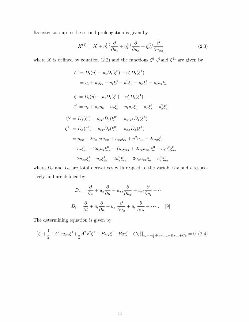
Its extension up to the second prolongation is given by

X(2) = X + η(1)t

∂

∂ut+ η(1)

x

∂

∂ux+ η(2)

xx

∂

∂uxx(2.3)

where X is defined by equation (2.2) and the functions ζ0, ζ1and ζ11 are given by

ζ0 = Dt(η)− utDt(ξ0)− uixDt(ξ

1)

= ηt + utηu − utξ0t − u2

t ξ0u − uxξ1

t − utuxξ1u

ζ i = Di(η)− utDi(ξ0)− uixDi(ξ

1)

ζ1 = ηx + uxηu − utξ0x − utuxξ0

u − uxξ1x − u2

xξ1u

ζ ij = Dj(ζi)− utxiDj(ξ

0)− uxixkDj(ξk)

ζ11 = Dx(ζ1)− utxDx(ξ

0)− uxxDx(ξ1)

= ηxx + 2ux etaxu + uxxηu + u2xηuu − 2utxξ

0x

− utξ0xx − 2utuxξ

0xu − (utuxx + 2uxutx)ξ

0u − utu2

xξ0uu

− 2uxxξ1x − uxξ1

xx − 2u2xξ

1xu − 3uxuxxξ

1u − u3

xξ1uu

where Dx and Dt are total derivatives with respect to the variables x and t respec-

tively and are defined by

Dx =∂

∂x+ ux

∂

∂u+ uxx

∂

∂ux+ uxt

∂

∂ut+ · · · .

Dt =∂

∂t+ ut

∂

∂u+ uxt

∂

∂ux+ utt

∂

∂ut+ · · · . [9]

The determining equation is given by

{ζ0+1

2+A2xuxxξ

1+1

2A2x2ζ11+Buxξ

1+Bxζ1−Cη}|ut=− 12A2x2uxx−Bxux+Cu = 0 (2.4)

31

The substitutions of ζ0t , ζ

1 and ζ11 in the determining equation yields that

ηt + (−1

2A2x2uxx −Bxux + Cu)(ηu − ξ0

t )− (−1

2A2x2uxx −Bxux + Cu)2ξ0

u−

uxξ1t − (−1

2A2x2uxx −Bxux + Cu)uxξ

1u + A2xuxxξ

1 +1

2A2x2ηxx + A2x2uxηxu

+1

2A2x2uxx(ηu − 2ξ1

x − 3uxξ1u) +

1

2A2x2u2

x(ηuu − 2ξ1ux)− A2x2utxξ

0x

− 1

2A2x2(−1

2A2x2uxx −Bxux + Cu)ξ0

xx − A2x2(−1


xu

− 1

2A2x2uxx(−

1


u −1

2A2x2(−1


uu

− 1

2A2x2u3

xξ1uu +Bvxξ

1 − A2x2utxuxξ0u +Bxux(ηu − ξ1

x)

−Bx(−1


x +Bxηx −Bxux(−1


u

−Bxu2xξ

1u − Cη = 0.

(2.5)

The solution of determining equation (2.5) provides an infinite dimensional vector

space of infinite symmetries of the equation (2.1) spanned by the operators

X1 = 2A2t2∂

∂t+ 2A2tx lnx

∂

∂x+ {(lnx−Dt)2 + 2A2Ct2 − A2t}u ∂

∂u

X2 = 2t∂

∂t+ x(lnx+Dt)

∂

∂x+ (Ct)u

∂

∂u

X3 =∂

∂t(2.6)

X4 = A2xt∂

∂x+ {lnx−Dt}u ∂

∂u

X5 = x∂

∂x

and

X6 = u∂

∂u, X∞ = g(t, x)

∂

∂u(2.7)

The function g(t, x) in (2.7) is an arbitrary solution of equation (2.1) and X∞ is an

infinite symmetry [9].

2.1.1 Finite symmetry transformations

The finite symmetry transformations

t = f(t, x, u, ε), x = g(t, x, u, ε), u = h(t, x, u, ε),

32

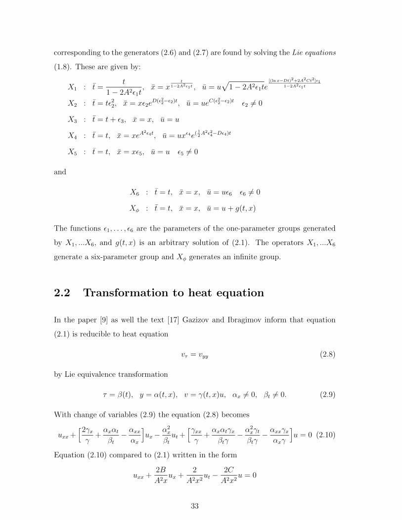
corresponding to the generators (2.6) and (2.7) are found by solving the Lie equations

(1.8). These are given by:

X1 : t =t

1− 2A2ε1t, x = x

t1−2A2ε1t , u = u

√1− 2A2ε1te

[(ln x−Dt)2+2A2Ct2]ε11−2A2ε1t

X2 : t = tε22, x = xε2eD(ε22−ε2)t, u = ueC(ε22−ε2)t ε2 6= 0

X3 : t = t+ ε3, x = x, u = u

X4 : t = t, x = xeA2ε4t, u = uxε4e( 1

2A2ε24−Dε4)t

X5 : t = t, x = xε5, u = u ε5 6= 0

and

X6 : t = t, x = x, u = uε6 ε6 6= 0

Xφ : t = t, x = x, u = u+ g(t, x)

The functions ε1, . . . , ε6 are the parameters of the one-parameter groups generated

by X1, ...X6, and g(t, x) is an arbitrary solution of (2.1). The operators X1, ...X6

generate a six-parameter group and Xφ generates an infinite group.

2.2 Transformation to heat equation

In the paper [9] as well the text [17] Gazizov and Ibragimov inform that equation

(2.1) is reducible to heat equation

vτ = vyy (2.8)

by Lie equivalence transformation

τ = β(t), y = α(t, x), v = γ(t, x)u, αx 6= 0, βt 6= 0. (2.9)

With change of variables (2.9) the equation (2.8) becomes

uxx +[2γxγ

+αxαtβt− αxxαx

]ux−

α2x

βtut +

[γxxγ

+αxαtγxβtγ

− α2xγtβtγ− αxxγx

αxγ

]u = 0 (2.10)

Equation (2.10) compared to (2.1) written in the form

uxx +2B

A2xux +

2

A2x2ut −

2C

A2x2u = 0

33

results in the system

α2x

βt= − 2

A2x2(2.11)

2γxγ

+αxαtβt− αxx

αx=

2B

A2x(2.12)

γxxγ

+αxαtγxβtγ

− α2xγtβtγ− αxxγx

αxγ= − 2C

A2x2(2.13)

Solving for α in (2.11) results in that

α(t, x) =ϕ(t)

Alnx+ ψ(t), βt = −1

2ϕ(t)2 (2.14)

with ϕ(t) and ψ(t) as arbitrary functions. The substitution of (2.14) in (2.12) results

in

γ(t, x) = ν(t)xBA2−

12

+ψtAϕ

+ψt

2A2ϕlnx

(2.15)

with an arbitrary function ν(t). The solution of (2.13) results in two possibilities,

either

ϕ =1

L−Kt, ψ =

M

L−Kt+N, K 6= 0,

and the function ν(t)

νtν

=M2K2

2(L−Kt)2− K

2(L−Kt)− A2

8+B

2− B2

2A2− C

or

ϕ = L, ψ = Mt+N, L 6= 0,

and the function ν(t)

νtν

=M2

L2− K

2(L−Kt)− A2

8+B

2− B2

2A2− C

with arbitrary constants K,L,M and N. This results in two different transformations

that associate (2.1) and (2.8). The first transformation is given by

y =lnx

A(L−Kt)+

M

L−Kt+N, τ = − 1

2K(L−Kt)+ P, K 6= 0

v = E√L−Kte[ MK2

2(L−Kt)−12

(BA−AB

)2−C]t−CtxBA2−

12

+ MKA(L−Kt)+ K ln x

2A2(L−Kt)u (2.16)

while the second transformation is

y =L

Alnx+Mt+N, τ = −L

2

2t+ P, L 6= 0

v = EeM2

2L2−12

(BA−AB

)2txBA2−

12

+ MALu (2.17)

34

The calculation presents two different transformations that associate (2.1) and (2.8)

([9]).

2.3 Invariant Solutions

One of the important components of classification of symmetry analysis is the con-

struction of invariant solutions. The paper ([9]) illustrates the calculation of invariant

solution by considering a subgroup and the procedure is applied to each operator and

the results are as follows: The one-parameter subgroup with the generator

X = X1 +X2 +X3 =∂

∂t+ x

∂

∂x+ u

∂

∂u.

provides invariants given by

I1 = t− lnx, I2 =u

x.

The invariant solution is of the form

I2 = φ(I1) or u = xφ(z), z = t− lnx.

The substitution of these invariants in equation (2.1) results in the equation with

constant coefficients given by

A

2φ′′ + (1−B − A

2)φ′ + (B − C)φ = 0

which is solvable. Applying the procedure to individual operators the results are as

follows:

X1 : u =1√te(

(ln x−Dt)2

2A2t+Ct)φ( ln x

t), φ′′ = 0

hence

u = (K1lnx

t32

+K2√t)e(

(ln x−Dt)2

2A2t+Ct)

X2 : u = eCtφ(lnx√t−D√t), A2φ′′ − zφ′ = 0, z =

lnx√t−D√t

whence

φ(z) = K1

∫ z

0

eµ2

2A2 dµ+K2

35

X3 : u = φ(x),1

2A2x2φ′′ +Bxφ′ − Cφ = 0.

The equation reduces to linear coefficients when z = lnx is introduced.

X4 : u = e((ln x−Dt)2

2A2t)φ(t), φ′ + (

1

2t− C)φ = 0

whence

φ =K√teCt

and hence

u =K√te(

(ln x−Dt)2

2A2t+Ct)

X5 : u = φ(t), φ′ − Cφ = 0 (2.18)

whence

u = KeCt (2.19)

K,K1, K2 are constants of integration, and

D = B − 1

2A2.

Operators X6, X∞ do not provide invariant solutions.

36

Chapter 3

Introduction of new method

This chapter presents the Symmetry Analysis of transformed one-dimensional and

two-dimensional Black-Scholes equations. The method employs a formula that we

shall henceforth be refer to as the Manale’s formula. The rationale and justification of

Manale’s formula is presented in Appendix A . We determine the symmetries from a

modified transformation with an infinitesimal ω → 0. We compute the Commutator

Table for operators in one-dimensional and determine invariant solutions for one

operator in each case. Graphical solutions are presented for the calculated solutions.

3.1 The transformed one-dimensional Black-Scholes

equation

We present a new method to Symmetry Analysis of (2.1) where we start with trans-

forming the equation in a different independent variable, r. The one-dimensional

Black-Scholes equation (2.1) is transformed using the following change of variables.

ux =∂u

∂x

xux =∂u∂xx

=∂u

∂ lnx

(3.1)

37

Let

r = lnx, then

∂r

∂x=

1

x∂x

∂r= x

(3.2)

We therefore express

xux =∂u

∂r(3.3)

Also,

uxx =∂

∂x(∂u

∂x)

x2uxx = x2 ∂

∂x

(∂u∂x

)= x

{ ∂∂xx

(∂u∂x

)}= x

{ ∂

∂ lnx

(∂u∂x

)}= x

{ ∂

∂r

(∂u∂x

)}= x

{ ∂

∂r

(1

x

∂u

∂ lnx

)}= x

{ ∂

∂r

(1

x

∂u

∂r

)}= x

{− 1

x2

∂r

∂x

∂u

∂r+

1

x

∂2u

∂r2

}= x

{− 1

x

∂u

∂r+

1

x

∂2u

∂r2

}= −∂u

∂r+∂2u

∂r2

(3.4)

Therefore

xux = ur

x2uxx = urr − ur(3.5)

where r is given by equation (3.2). We substitute equation (3.5) in equation (2.1)

and define

D = B − A2

2,

then the Black-Scholes one dimensional equation transforms to

ut +1

2A2urr +Dur − Cu = 0. (3.6)

38

3.2 Solution of determining equation for (3.6)

The infinitesimal generator for point symmetry admitted by equation (3.6)

is of the form

X = ξ1(t, r)∂

∂t+ ξ2(t, r)

∂

∂r+ η(t, r)

∂

∂u(3.7)

The extension of the equation up to the second prolongation is given by

X(2) = X + η(1)t

∂

∂ut+ η(1)

r

∂

∂ur+ η(2)

rr

∂

∂urr(3.8)

where X is defined by equation (3.7).


η(1)t +

1

2A2η(2)

rr +Dη(1)r − Cη = 0 (3.9)

when

urr = (− 2

A2)[ut +Dur − Cu] (3.10)

where we define the following from ([6],[15])

η = fu+ g

η(1)t = gt + ftu+ [f − ξ1

t ]ut − ξ2t ur

η(1)r = gr + fru+ [f − ξ2

r ]ur − ξ1rut

η(2)rr = grr + frru+ [2fr − ξ2

rr]ur − ξ1rrut

+ [f − 2ξ2r ]urr − 2ξ1

rutr

(3.11)

The substitutions of η(1)t , η

(1)r and η

(2)rr in the determining equation yields that

gt + ftu+ [f − ξ1t ]ut − ξ2

t ur + (1

2A2){grr + frru+ [2fr − ξ2

rr]ur

− ξ1rrut + [f − 2ξ2

r ](−2

A2[ut +Dur − Cu])− 2ξ1

rutr}

+ (D)[gr + fru+ [f − ξ2r ]ur − ξ1

rut]− Cfu− Cg = 0

(3.12)

We set the coefficients of ur, utr, ut and those free of these variables to zero. We thus

39

have the following monomials which we termed defining equations

utr : ξ1r = 0, (3.13)

ut : −ξ1t + 2ξ2

r = 0 (3.14)

ur : −ξ2t + A2fr +Dξ2

r −1

2A2ξ2

rr = 0, (3.15)

u0r : gt +

1

2A2grr +Dgr − Cg = 0, (3.16)

u : ft +1

2A2frr +Dfr − 2Cξ2

r = 0 (3.17)

From defining equations (3.13) and (3.14) we have that

ξ2rr = 0 (3.18)

Thus

ξ2 = ar + b (3.19)

which can be expressed using Manale’s formula with infinitesimal ω as

ξ2 =a sin(ωr

i) + bφ cos(ωr

i)

−iω, where φ = sin(

ω

i), (3.20)

and a and b are arbitrary functions of t. We differentiate equation (3.20) with respect

to r and t and obtain

the following equations

ξ2r = a cos(

ωr

i)− bφ sin(

ωr

i), (3.21)

ξ2rr =

−ωi

a sin(ωr

i)− ω

ib φ cos(

ωr

i), (3.22)

ξ2t =

a sin(ωri

) + bφ cos(ωri

)

−iω(3.23)

and from defining equation (3.14) we have ξ1t = 2ξ2

r which implies that

ξ1 = 2at cos(ωr

i)− 2btφ sin(

ωr

i) + C. (3.24)

We substitute equations (3.21), (3.22) and (3.23)

in the defining equation (3.15) to get the expression for fr given by

fr = cos(ωr

i){− ωbφ

2i− bφ

A2iω− Da

A2

}+ sin(

ωr

i){− ωa

2i− a

A2iω+Dbφ

A2

}(3.25)

40

Integrating equation (3.25) with respect to r gives the expression for f

f = sin(ωr

i){− bφ

2− bφ

A2ω2− Dia

A2ω

}+ cos(

ωr

i){a

2+

a

A2ω2− Dibφ

A2ω

}+ k(t) (3.26)

We use equations (3.25) and (3.26) to get expressions for frr and ft given by

frr = sin(ωr

i){− ω2bφ

2− bφ

A2+Daω

A2i

}+ cos(

ωr

i){ω2a

2+

a

A2+Dbωφ

A2i

}(3.27)

and

ft = sin(ωr

i){− bφ

2− bφ

A2ω2− Dia

A2ω

}+ cos(

ωr

i){ a

2+

a

A2ω2− Diaφ

A2ω

}+ k′(t) (3.28)

We substitute equations (3.21), (3.25), (3.27) and (3.28) into the defining equation

(3.17) and solve the equation

sin(ωr

i){− bφ

2− bφ

A2ω2− Dia

A2ω+ 2Cbφ

}+ cos(

ωr

i){ a

2+

a

A2ω2− Dibφ

A2ω− 2Ca

}+ k′(t) + sin(

ωr

i){− bA2ω2φ

4− bφ

2+Daω

2i

}+ cos(

ωr

i){aA2ω2

4+a

2+Dbωφ

2i

}+

cos(ωr

i){− Dbωφ

2i− Dbφ

A2iω− D2a

A2

}+ sin(

ωr

i){− Daω

2i− Da

A2iω+D2bφ

A2

}= 0

(3.29)

We collect all the coefficients of sine function together and equate

them to zero. A similar step is taken with the cosine function.

For the coefficients of sine function we have:

− bφ

2− bφ

A2ω2− Dia

A2ω− bA2ω2φ

4− bφ

2− Daω

2i

+Daω

2i− Da

A2ωi− D2bφ

A2+ 2Cbφ = 0

(3.30)

which simplifies to a second-order ordinary linear differential equation

b+ bA2ω2 +bA4ω4

4− D2b

A2+ 2CA2ω2b = 0 (3.31)

Solving equation (3.31) we proceed as follows. Let

β =A2ω2

2, and k1 = −D

2

A2− 2C (3.32)

We also set

α1 = bβ2 − k, then α1 = bβ2, α1 = bβ2 (3.33)

41

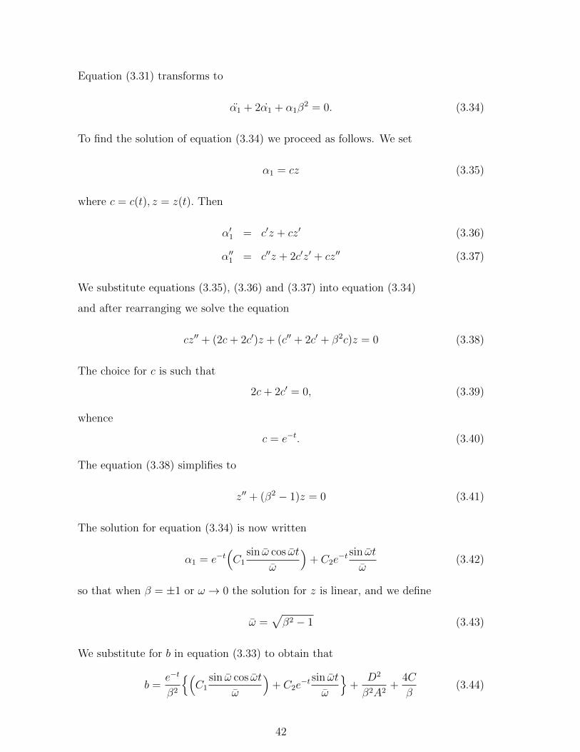
Equation (3.31) transforms to

α1 + 2α1 + α1β2 = 0. (3.34)

To find the solution of equation (3.34) we proceed as follows. We set

α1 = cz (3.35)

where c = c(t), z = z(t). Then

α′1 = c′z + cz′ (3.36)

α′′1 = c′′z + 2c′z′ + cz′′ (3.37)

We substitute equations (3.35), (3.36) and (3.37) into equation (3.34)

and after rearranging we solve the equation

cz′′ + (2c+ 2c′)z + (c′′ + 2c′ + β2c)z = 0 (3.38)

The choice for c is such that

2c+ 2c′ = 0, (3.39)

whence

c = e−t. (3.40)

The equation (3.38) simplifies to

z′′ + (β2 − 1)z = 0 (3.41)

The solution for equation (3.34) is now written

α1 = e−t(C1

sin ω cos ωt

ω

)+ C2e

−t sin ωt

ω(3.42)

so that when β = ±1 or ω → 0 the solution for z is linear, and we define

ω =√β2 − 1 (3.43)

We substitute for b in equation (3.33) to obtain that

b =e−t

β2

{(C1

sin ω cos ωt

ω

)+ C2e

−t sin ωt

ω

}+

D2

β2A2+

4C

β(3.44)

42

Similarly for the coefficients of the cosine function we have

a

2+

aφ

A2ω2− Dibφ

A2ω+aA2ω2φ

4+a

2+Dbωφ

2i− Dbωφ

2i

− Dbφ

A2ωi− D2a

A2+ 2aC = 0

(3.45)

which simplifies to a second-order ordinary linear differential equation

a+ aA2ω2 +aA4ω4

4− aD2

A2− 2aA2ω2C = 0 (3.46)

Solving equation (3.46) we find the solution for a to be

a =e−t

β2

{(C3

sin ω cos ωt

ω

)+ C4

sin ωt

ω

}+

D2

β2A2− 4C

β(3.47)

and we also have that

k′(t) = 0 ⇒ k(t) = C5 (3.48)

We differentiate equations (3.44) and (3.47) to obtain expressions for a and b

a = −e−t

β2

(C3

sin ω cos ωt

ω+ C4

sin ωt

ω

)+e−t

β2

(− C3 sin ω sin ωt+ C4 cos ωt

)(3.49)

Similarly

b = −e−t

β2

(C1

sin ω cos ωt

ω+ C2

sin ωt

ω

)+e−t

β2

(− C1 sin ω sin ωt+ C2 cos ωt

)(3.50)

We substitute equations (3.32),(3.44),(3.47),(3.48),(3.49) and (3.50) into equation

(3.26) and get the expression for f given as

f = sin(ωr

i){− C1φe

−t sin ω cos ωt

2β2ω− C2φe

−t sin ωt

2β2ω− D2φ

2β3A2− 4Cφ

β

+C1φe

−t sin ω cos ωt

2β3ω+C2φe

−t sin ωt

2β3ω+C1φe

−t sin ω cos ωt

2β3

− C2φe−t cos ωt

2β3− C3Diωe

−t sin ω cos ωt

2β3− C4Diωe

−t sin ωt

2β3− D3iω

2β3A2

}+ cos(

ωr

i){C3e

−t sin ω cos ωt

2β2ω+C4e

−t sin ωt

2β2ω+

D2

2β3A2− 4Cφ

β

− C3e−t sin ω cos ωt

2β3ω− C4e

−t sin ωt

2β3ω− C3e

−t sin ω sin ωt

2β3

− C4e−t cos ωt

2β3− C1φDiωe

−t sin ω cos ωt

2β3

− C2φDiωe−t sin ωt

2β3− D3φiω

2β3A2

}+ C5

43

3.2.1 Infinitesimals for equation (3.6)

The linearly independent solutions of the defining equations (3.12) lead to the in-

finitesimals

ξ1 = cos(ωri

){2te−t

β2ω

{(C3 sin ω cos ωt

)+ C4 sin ωt

}+

2tD2

β2A2

}− sin

(ωri

){2tφe−t

β2ω

{(C1 sin ω cos ωt

)+ C2 sin ωt

}+

2tφD2

β2A2

}− 8Ct

βcos(ωri

)+

8Ctφ

βsin(ωri

)+ C6

(3.51)

ξ2 = sin(ωri

){ e−t

−β2ωωi

(C3 sin ω cos ωt+ C4 sin ωt

)− D2

iωβ2A2

}+ cos

(ωri

){ e−tφ

−β2ωωi

(C1 sin ω cos ωt− C2 sin ωt

)− D2φ

iωβ2A2

}+

4Ci

ωβsin(ωri

)+

4Ciφ

ωβcos(ωri

) (3.52)

f = sin(ωr

i){− C1φe

−t sin ω cos ωt

2β2ω− C2φe

−t sin ωt

2β2ω− D2φ

2β3A2− 4Cφ

β

+C1φe

−t sin ω cos ωt

2β3ω+C2φe

−t sin ωt

2β3ω+C1φe

−t sin ω cos ωt

2β3

− C2φe−t cos ωt

2β3− C3Diωe

−t sin ω cos ωt

2β3− C4Diωe

−t sin ωt

2β3− D3iω

2β3A2

}+ cos(

ωr

i){C3e

−t sin ω cos ωt

2β2ω+C4e

−t sin ωt

2β2ω+

D2

2β3A2− 4Cφ

β

− C3e−t sin ω cos ωt

2β3ω− C4e

−t sin ωt

2β3ω− C3e

−t sin ω sin ωt

2β3

− C4e−t cos ωt

2β3− C1φDiωe

−t sin ω cos ωt

2β3

− C2φDiωe−t sin ωt

2β3− D3φiω

2β3A2

}+ C5

(3.53)

44

3.2.2 The symmetries for equation (3.6)

According to (3.12), the infinitesimals: (3.53), (3.51) and (3.52), lead to the genera-

tors

X1 =(− 2te−tφ

β2ωsin ω cos ωt sin

(ωri

)) ∂∂t

+( e−tiφβ2ωω

sin ω cos ωt cos(ωri

)) ∂∂r

+{− e−tφ

2β2ωsin ω cos ωt sin

(ωri

)+e−tφ


(ωri

)+e−tφ

2β3sin ω cos ωt sin

(ωri

)− Diφωe−t sin ω cos ωt

2β3cos(ωri

)}u∂

∂u

(3.54)

X2 =(− 2te−tφ

β2ωsin ωt sin

(ωri

)) ∂∂t−( e−tiφβ2ωω

sin ωt cos(ωri

)) ∂∂r

+{− e−tφ

2β2ωsin ωt sin

(ωri

)+e−tφ

2β3ωsin ωt sin

(ωri

)− e−tφ

2β3cos ωt sin

(ωri

)− Diφωe−t sin ωt

2β3cos(ωri

)}u∂

∂u

(3.55)

X3 =(2te−t

β2ωsin ω cos ωt cos

(ωri

)) ∂∂t

+( e−ti

β2ωωsin ω cos ωt cos

(ωri

)) ∂∂r

+{ e−t

2β2ωsin ω cos ωt cos

(ωri

)− e−t


(ωri

)− e−t

2β3sin ω sin ωt cos

(ωri

)− Diωe−t sin ω cos ωt

2β3sin(ωri

)}u∂

∂u

(3.56)

X4 =(2te−tφ

β2ωsin ωt cos

(ωri

)) ∂∂t

+( e−tiφβ2ωω

sin ωt sin(ωri

)) ∂∂r

+{ e−t

2β2ωsin ωt cos

(ωri

)− e−t

2β3ωsin ωt cos

(ωri

)+e−t

2β3cos ωt cos

(ωri

)− Diωe−t sin ωt

2β3sin(ωri

)}u∂

∂u

(3.57)

X5 =2tD2

β2A2

(cos(ωri

)− φ sin

(ωri

)) ∂∂t

+D2

ωβ2A2

(φ cos

(ωri

)+ sin

(ωri

)) ∂∂r− D2iω

2β3A2

(sin(ωri

)+ φ cos

(ωri

)+D sin

(ωri

)+Dφ cos

(ωri

))u∂

∂u

(3.58)

X6 = u∂

∂u(3.59)

45

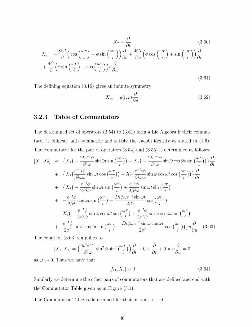
X7 =∂

∂t(3.60)

X8 = −8Ct

β

(cos(ωri

)+ φ sin

(ωri

)) ∂∂t

+4Ct

βω

(φ cos

(ωri

)+ sin

(ωri

)) ∂∂r

+4C

β

(φ sin

(ωri

)− cos

(ωri

))u∂

∂u

(3.61)

The defining equation (3.16) gives an infinite symmetry

X∞ = g(t, r)∂

∂u(3.62)

3.2.3 Table of Commutators

The determined set of operators (3.54) to (3.61) form a Lie Algebra if their commu-

tator is bilinear, anti symmetric and satisfy the Jacobi identity as stated in (1.6).

The commutator for the pair of operators (3.54) and (3.55) is determined as follows:

[X1, X2] ={X1

(− 2te−tφ

β2ωsin ωt sin

(ωri

))−X2

(− 2te−tφ

β2ωsin ω cos ωt sin

(ωri

))} ∂∂t

+{X1

( e−tiφβ2ωω

sin ωt cos(ωri

))−X2

( e−tiφβ2ωω

sin ω cos ωt cos(ωri

))} ∂∂r

+{X1

(− e−tφ

2β2ωsin ωt sin

(ωri

)+e−tφ

2β3ωsin ωt sin

(ωri

)+ −e

−tφ

2β3cos ωt sin

(ωri

)− Diφωe−t sin ωt

2β3cos(ωri

))− X2

(− e−tφ


(ωri

)+e−tφ


(ωri

)+

e−tφ

2β3sin ω cos ωt sin

(ωri

)− Diφωe−t sin ω cos ωt

2β3cos(ωri

))}u∂

∂u(3.63)

The equation (3.63) simplifies to

[X1, X2] =(4t2e−2t

β4ωsin2 ω sin2

(ωri

)) ∂∂t

+ 0× ∂

∂r+ 0× u ∂

∂u= 0

as ω → 0. Thus we have that

[X1, X2] = 0 (3.64)

Similarly we determine the other pairs of commutators that are defined and end with

the Commutator Table given as in Figure (3.1).

The Commutator Table is determined for that instant ω → 0.

46

[, ] X1 X2 X3 X4 X5 X6 X8

X1 0 0 0 0 0 0 0

X2 0 0 0 0 0 0 0

X3 0 0 0 0 0 0 0

X4 0 0 0 0 0 0 0

X5 0 0 0 0 0 0 0

X6 0 0 0 0 0 0 0

X8 0 0 0 0 0 0 0

Figure 3.1: Commutator Table

3.3 Invariant Solution for equation (3.6)

We consider the symmetry given by equation (3.56). The invariants are determined

from solving the equation

X3I =(2te−t

β2ωsin ω cos ωt cos

(ωri

))∂I∂t

+( e−ti

β2ωωsin ω cos ωt cos

(ωri

))∂I∂r

+{ e−t


(ωri

)− e−t


(ωri

)− e−tφ

2β3sin ω sin ωt cos

(ωri

)− Diωe−t sin ω cos ωt

2β3sin(ωri

)}u∂I

∂u= 0

(3.65)

The characteristic equation of (3.65) is given by

dt

2te−t sin ω cos ωt cos

(ωri

)β2ω

=dr

e−ti sin ω sin ωt cos

(ωri

)β2ωω

=du

ue−tK(3.66)

where

K ={sin ω cos ωt cos

(ωri

)2β2ω

−sin ω cos ωt cos

(ωri

)2β3ω

−sin ω sin ωt cos

(ωri

)2β3

−Diω sin ω cos ωt sin

(ωri

)2β3

} (3.67)

From equation (3.66) we have that

dt

2te−t sin ω cos ωt cos

(ωri

)β2ω

=dr


(ωri

)β2ωω

(3.68)

47

simplifies todt

t= 2

ω

idr (3.69)

whose solution is

t = Ce2ωri (3.70)

The first invariant is given by

ψ1 =e

2ωri

t(3.71)

From equation (3.66) we also have that

dr


(ωri

)β2ωω

=du

Kue−t(3.72)

where K is given by (3.67). Equation (3.72) simplifies to

(β − 1− ω −Diωω tan(ω

i)

2β)(ω

i)dr =

du

u(3.73)

We integrate equation (3.73) and obtain

βωr

2βi− ωr

2βi− ωωr

2βi−Dωω ln cos(ωr

i)|

2β+ C = lnu (3.74)

We approximate

βωr

2βi− ωr

2βi− ωωr

2βi−Dωω ln cos(ωr

i)|

2β≈ ωr

i(3.75)

Integrating equation (3.72) we obtain

u

eωri

= C (3.76)

The equation (3.76) simplifies tou

eωri

= ψ2 (3.77)

which is our second invariant. If we define

ψ2 = ϕ(ψ1) (3.78)

where ψ1 is given by equation (3.71), then an invariant solution is given by

u = eωri ϕ(ψ1) (3.79)

48

We differentiate equation (3.79) with respect to t and twice with respect

to r and get the following expressions for ut, ur and urr.

ut = −2ωr

i

e3ωri

t2ϕ′(ψ1) (3.80)

ur =ω

ieωri ϕ(ψ1) +

2ω

ite

3ωri ϕ′(ψ1) (3.81)

urr =− ω2eωri ϕ(ψ1)− 2ω2

te

3ωri ϕ′(ψ1)− 6ω2

te

3ωri ϕ′(ψ1)

−−4ω2

t2e

5ωri ϕ′′(ψ1)

(3.82)

We substitute equations (3.80), (3.81) and (3.82) into the

original equation (3.6) and get the following equation

− 2ωr

i

e3ωri

t2ϕ′(ψ1)− ω2e

ωri ϕ(ψ1)− A2ω2

te

3ωri ϕ′(ψ1)− 3A2ω2

te

3ωri ϕ′(ψ1)

− 2A2ω2

t2e

5ωri ϕ′′(ψ1) +

Dω

ieωri ϕ(ψ1) +

2Dω

ite

3ωri ϕ′(ψ1)− Ce

ωri ϕ(ψ1) = 0

(3.83)

Equation (3.83) is a second order equation in ϕ(ψ1). We rearrange it in

the order of derivatives of h(ψ1), and apply equation (3.32)

− 4β

t2e

5ωri ϕ′′(ψ1)− ϕ′(ψ1){2ωr

i

e3ωri

t2+

4β

te

3ωri +

6β

te

3ωri

− 2Dω

ie

3)ωri }+ ϕ(ψ1){Dkω

iteωri − βe

ωri − Ce

ωri } = 0

(3.84)

Letting ω → 0 equation (3.84) simplifies to

−4β

t2ϕ′′(ψ1)− 4β

tϕ′(ψ1)− 6β

tϕ′(ψ1)− βϕ(ψ1)− Cϕ(ψ1) = 0 (3.85)

which can be simplified to

4βϕ′′(ψ1)

t2+

10βϕ′(ψ1)

t+ (β + C)ϕ(ψ1) = 0. (3.86)

We eliminate t from equation (3.86) by applying the following change of variables.

From equation (3.71) we let

dλ = tdψ1,

ϕ(ψ1) = h(3.87)

then

ϕ′(ψ1) = tϕλ (3.88)

49

and

ϕ′′(ψ1) = ddψ1{tϕλ} (3.89)

= dtdψ1

ϕλ + tdϕλdψ1

= dtdψ1

ϕλ + t dϕλ1tdλ

= t2{hλλ − ϕλe−2ωri }

For ω → 0 equation (3.89) simplifies to

ϕ′′(ψ1) = t2{ϕλλ − ϕλ} (3.90)

The substitution of equations (3.88), (3.90) transforms equation (3.86) to

4βϕλλ + 6βϕλ + (β + C)ϕ = 0. (3.91)

The solution to equation (3.91) is given by

ϕ = C1e(−3β−

√9β2−4β(β+C)

4β)(λ) + C2e

(−3β+

√9β2−4β(β+C)

4β)(λ) (3.92)

Thus the invariant solution is

u = eωri {C1e

(−3β−

√9β2−4β(β+C)

4β)(λ) + C2e

(−3β+

√9β2−4β(β+C)

4β)(λ)} (3.93)

However the equation (3.93) can be expressed as

u = eωri {C1e

(−3β−i

√−(9β2−4β(β+C))

4β)(λ) + C2e

(−3β+i

√−(9β2−4β(β+C))

4β)(λ)} (3.94)

This simplifies to

u = eωri {C1e

−34λe−i∆λ + C2e

−34λei∆λ}

where ∆ =

√−(9β2 − 4β(β + C))

4β

(3.95)

Since ∆ < 0, we express equation (3.95) as

u = eωri {C1e

−34λ sin(∆λ) + C2e

−34λ cos(∆λ)} (3.96)

We however advance the same reason that for equation (3.96) to return

to the linear form as ∆→ 0 it has to be transformed to be

u = eωri {C1e

−34λ sin(∆λ)

−i∆+ C2e

−34λφ

cos(∆λ)

−i∆}

where φ = sin(∆

i)

(3.97)

50

0 2 4 6 8 10

0

5

10

15

20

Figure 3.2: Plot for the solution (3.100) with dependent variable u represented on

the vertical axis and independent variable t represented on the horizontal axis

3.3.1 Solutions for equation 3.97

This equation (3.97) has some few solutions as ω → 0. We recall that

λ = t∫ ψ2

ψ1d e

2ωri

t(3.98)

= e2ωri

∫ ψ2

ψ1

d 1t1t

= C0 − e2ωri ln t

Solution 1

u = Aeωri e−

34λ sin(∆λ)−i∆ (3.99)

= Aeωri e(C0+ 3

4e2ωri ln t) sin(∆(C0−e

2ωri ln t))

−i∆

as ω → 0, the solution becomes

u =3√t4 (3.100)

51

Solution 2

u = Aeωri e−

34λ sin(∆λ)−i∆ (3.101)

= A(cos(ωr)− sin(ωr)e( 34λ) sin(∆λ)−i∆


u = Ae( 34λ) sin(∆λ)

−i∆(3.102)

This result is comparable to (2.19).

0 2 4 6 8 10

0

200

400

600

800

Figure 3.3: Plot for solution (3.102) with dependent variable u represented on the

vertical axis and independent variable λ represented on the horizontal axis

52

Solution 3

u = Aωeωri e−

34

∫ ψ1+ωψ1

dψ1sin(∆

∫ ψ1+ω

ψ1tdψ1)

−i∆ω

= Aωeωri e−

34

∫ ψ1+ωψ1

dψ1d

dω[sin(∆

∫ ψ1+ω

ψ1tdψ1)

−i∆]

= Aωeωri e−

34

∫ ψ1+ωψ1

dψ1dψ1

dω

d

dω[sin(∆

∫ ψ1+ω

ψ1tdψ1)

−i∆]

= Aωeωri e−

34

∫ ψ1+ωψ1

dψ12re

2ωri

it[cos(∆

∫ ψ1+ω

ψ1dψ1)

−i∆]t

= Aωeωri e−

34

∫ ψ1+ωψ1

dψ12re

2ωri

itt

= Aω2re

3ωri

i

(3.103)

But

ωe3ωri = ω cos(3ωr)− iω sin(3ωr)

ω2e3ωri = ω2 cos(3ωr)− iω2 sin(3ωr)

=1

ω{ω3 cos(3ωr)− iω3 sin(3ωr)}

(3.104)

and

ω3r2 cos(ωr

i) = ω2e3ωr

ω2e3ωri =

1

ω

1

r2ω2e3ωr

e3ωri =

1

ω

1

r2e3ωr

(3.105)

We substitute in equation (3.103) and obtain

u = Aω2r

i

1

ω

1

r2e3ωr (3.106)


u =2A

ir(3.107)

53

0 2 4 6 8 10

0.5

1.0

1.5

2.0

2.5

Figure 3.4: Plot for solution (3.107) with dependent variable u represented on the

vertical axis and independent variable r represented on the horizontal axis

3.4 Two-Dimensional Black-Scholes Equation

3.4.1 Transformed two-dimensional Black-Scholes Equation

A two-dimensional Black-Scholes equation is given by

ut +1

2A2

11x2uxx +

1

2A2

22y2uyy +B1xux +B2yuy − Cu = 0. (3.108)

We apply change of variables similar to (3.4), and use equation (3.5) to reduce

equation (3.108) to

ut +1

2A2

11urr +1

2A2

22uss +D1ur +D2us − Cu = 0. (3.109)

where

D1 = B1 −A2

11

2

D2 = B2 −A2

22

2

(3.110)

The infinitesimal generator for point symmetry admitted by equation (3.109) is of

the form

X = ξ1(t, r, s)∂

∂t+ ξ2(t, r, s)

∂

∂r+ ξ3(t, r, s)

∂

∂s+ η(t, r, s)

∂

∂u(3.111)

54

Its first and second prolongations are given by

X(2) = X + η(1)t

∂

∂ut+ η(1)

r

∂

∂ur+ η(1)

s

∂

∂us+ η(2)

rr

∂

∂urr+ η(2)

ss

∂

∂uss(3.112)

where X is defined by equation (3.111).

3.4.2 Solution for determining equation for (3.109)

The determining equation for (3.109) is given by

η(1)t +

1

2A2

11η(2)rr +

1

2A2

22η(2)ss +D1η

(1)r +D2η

(1)s − Cη = 0 (3.113)

when

ut = −1

2A2

11urr −1

2A2

22uss −D1ur −D2us + Cu (3.114)

where we define the following from ([5])

η = fu+ g

η(1)t = gt + ftu+ [f − ξ1

t ]ut − ξ2t ur − ξ3

t us

η(1)r = gr + fru+ [f − ξ2

r ]ur − ξ1rut − ξ3

rus

η(1)s = gs + fsu+ [f − ξ3

s ]us − ξ1sut − ξ2

sur

η(2)rr = grr + frru+ [2fr − ξ2

rr]ur − ξ1rrut − ξ3

rrus + [f − 2ξ2r ]urr

− 2ξ1rutr − 2ξ3

rurs

η(2)ss = gss + fssu+ [2fs − ξ3

ss]us − ξ1ssut − ξ2

ssur + [f − 2ξ3s ]uss

− 2ξ1suts − 2ξ2

surs

(3.115)

55

The substitutions of η(1)t , η

(1)r , η

(1)r , η

(2)rr and η

(2)ss in the determining equation (3.113)

yield that

gt + ftu+ [f − ξ1t ](−

1

2A2

11urr −1

2A2

22uss −D1ur −D2us + Cu)

− ξ2t ur − ξ3

t us +1

2A2

11{grr + frru+ [2fr − ξ2rr]ur

− ξ1rr(−

1

2A2

11urr −1

2A2

22uss −D1ur −D2us + Cu)− ξ3rrus

+ [f − 2ξ2r ]urr − 2ξ1

rutr − 2ξ3rurs}+

1

2A2

22{gss + fssu+ [2fs − ξ3ss]us

− ξ1ss(−

1

2A2

11urr −1

2A2

22uss −D1ur −D2us + Cu)− ξ2ssur + [f − 2ξ3

s ]uss

− 2ξ1suts − 2ξ2

surs}+D1{gr + fru+ [f − ξ2r ]ur

− ξ1r (−

1

2A2

11urr −1

2A2

22uss −D1ur −D2us + Cu)− ξ3rus}

+D2{gs + fsu+ [f − ξ3s ]us

− ξ1s (−

1

2A2

11urr −1

2A2

22uss −D1ur −D2us + Cu)− ξ2sur}

− Cfu− Cg = 0

(3.116)

We set the coefficients of utr, uts, uts, urr, uss, ur, us, u and those free of these variables

to zero. We thus have the following defining equations

utr : ξ1r = 0, (3.117)

uts : ξ1s = 0, (3.118)

urs : ξ2s + ξ3

r = 0, (3.119)

urr :1

2ξ1t − ξ2

r = 0, (3.120)

uss :1

2ξ1t − ξ3

s = 0, (3.121)

ur : −ξ2t + A2

11fr −D1ξ2r −

1

2A2

11ξ2rr +D1ξ

1t = 0, (3.122)

us : −ξ3t + A2

22fs −1

2A2

22ξ3ss −D2ξ

3s +D2ξ

1t = 0 (3.123)

u : ft +1

2A2

11frr +1

2A2

22fss +D1fr +D2fs − Cξ1t = 0, (3.124)

u0 : gt +1

2A2

11grr +1

2A2

22gss +D1gr +D2gs − Cg = 0 (3.125)

From defining equation (3.120) we have that

ξ2rr = 0 (3.126)

56

Thus

ξ2 = ar + b (3.127)


ξ2 =a sin(ωr

i) + bφ cos(ωr

i)

−iωwhere φ = sin(

ω

i),

(3.128)

and also a and b are arbitrary functions of t. Similarly, from defining equation (3.121)

we have that

ξ3ss = 0 (3.129)

This implies that

ξ3 = cs+ h (3.130)


ξ3 =c sin(ωs

i) + hφ cos(ωs

i)


ω

i),

(3.131)

and also c and h are arbitrary functions of t. We differentiate equation (3.128) with

respect to r and t and obtain expressions for ξ2t , ξ

2r , and ξ2

rr

ξ2t =

a sin(ωri

) + bφ cos(ωri

)

−iω(3.132)

ξ2r = a cos(

ωr

i)− bφ sin(

ωr

i), (3.133)

ξ2rr =

−ωi

a sin(ωr

i)− ω

ib φ cos(

ωr

i), (3.134)

Similarly we differentiate equation (3.131) with respect to s and t and obtain expres-

sions for ξ3t , ξ

3s , and ξ3

ss

ξ3t =

c sin(ωsi

) + hφ cos(ωsi

)

−iω(3.135)

ξ3s = c cos(

ωs

i)− hφ sin(

ωs

i), (3.136)

ξ3ss =

−ωi

c sin(ωs

i)− ω

ih φ cos(

ωs

i). (3.137)

57

The defining equations (3.120) and (3.121) imply that ξ1t = 2ξ2

r and ξ1t = 2ξ3

s which

translates to that

ξ1t = 2{a cos(

ωr

i) + c cos(

ωs

i)} − 2φ{b sin(

ωr

i) + h sin(

ωs

i)}. (3.138)

The integration of equation (3.138) results in the infinitesimal

ξ1 = 2t{a cos(ωr

i) + c cos(

ωs

i)} − 2tφ{b sin(

ωr

i) + h sin(

ωs

i)}+ C. (3.139)

We substitute equations (3.132), (3.133), (3.134) and (3.138) into the defining equa-

tion (3.122) to get the expression for fr given by

fr = cos(ωr

i){− bωφ

2i− bφ

A211iω

− D1a

A211

}+ sin(

ωr

i){− ωa

2i− a

A211iω

+D1φb

A211

}− 2D1c

A211

cos(ωs

i) +

2D1φh

A211

sin(ωs

i)

(3.140)

Similarly we substitute equations (3.135), (3.136), (3.137) and (3.138) into the defin-

ing equation (3.123) to get the expression for fs given by

fs = cos(ωs

i){− ωhφ

2i− hφ

A222iω

− D2c

A222

}

+ sin(ωs

i){− ωc

2i− c

A222iω

+D2hφ

A222

}− 2D2a

A222

cos(ωr

i) +

2D2φb

A222

sin(ωr

i)

(3.141)

Integrating equation (3.140) with respect to r gives

sin(ωr

i){− bφ

2− bφ

A211ω

2− D1ia

A211ω

}+ cos(

ωr

i){a

2+

a

A211ω

2− D1ibφ

A211ω

}− 2D1cr

A211

cos(ωs

i) +

2D1hrφ

A211

sin(ωs

i) + k(t)

(3.142)

Similarly integrating equation (3.140) with respect to s yields

sin(ωs

i){− hφ

2− hφ

A222ω

2− D2ic

A222ω

}+ cos(

ωs

i){ c

2+

c

A222ω

2− D2ihφ

A222ω

}− 2D2as

A222

cos(ωr

i) +

2D2bsφ

A222

sin(ωr

i) + k(t)

(3.143)

58

Reconciling equations (3.142) and (3.143) we get the expression for f given by

f = sin(ωr

i){− bφ

2− bφ

A211ω

2− D1ia

A211ω

+2D2bsφ

A222

}+ cos(

ωr

i){a

2+

a

A211ω

2− D1ibφ

A211ω− 2D2as

A222

}+ sin(

ωs

i){− hφ

2− hφ

A222ω

2− D2ic

A222ω

+2D1hrφ

A211

}+ cos(

ωs

i){ c

2+

c

A222ω

2− D2ihφ

A222ω− 2D1cr

A211

}+ k(t)

(3.144)

We differentiate equation (3.144) to obtain expressions for ft, frr and fss.

ft = sin(ωr

i){− bφ

2− bφ

A211ω

2− D1ia

A211ω

+2D2bsφ

A222

}+ cos(

ωr

i){ a

2+

a

A211ω

2− D1ibφ

A211ω− 2D2as

A222

}+ sin(

ωs

i){− hφ

2− hφ

A222ω

2− D2ic

A222ω

+2D1hrφ

A211

}+ cos(

ωs

i){ c

2+

c

A222ω

2− D2ihφ

A222ω− 2D1cr

A211

}+ k′(t)

(3.145)

frr = sin(ωr

i){− ω2bφ

2− bφ

A211

+D1ωa

A211i

}+ cos(

ωr

i){ω2a

2+

a

A211

+D1bωφ

iA211

} (3.146)

fss = sin(ωs

i){− ω2hφ

2− hφ

A222

− D2ωc

A222i

}+ cos(

ωs

i){ω2c

2+

c

A222

+D2eωφ

iA222

} (3.147)

59

We substitute equations (3.133), (3.136) (3.138), (3.140), (3.142),(3.148), (3.149) and

(3.150) into the defining equation (3.124) and solve the equation

sin(ωr

i){− bφ

2− bφ

A211ω

2− D1ia

A211ω

+2D2bsφ

A222

}+ cos(

ωr

i){ a

2+

a

A211ω

2

− D1ibφ

A211ω− 2D2as

A222

}+ sin(

ωs

i){− hφ

2− hφ

A222ω

2− D2ic

A222ω

+2D1hrφ

A211

}+ cos(

ωs

i){ c

2+

c

A222ω

2− D2ihφ

A222ω− 2D1cr

A211

}+ sin(

ωr

i){− A2

11ω2bφ

4− bφ

2+D1ωa

2i

}+ cos(

ωr

i){A2

11ω2a

4+a

2+D1bωφ

2i

}+ sin(

ωs

i){− A2

22ω2eφ

4− hφ

2+D2ωc

2i

}+ cos(

ωs

i){A2

22ω2c

4+c

2+D2hωφ

2i

}+ cos(

ωr

i){− D1bωφ

2i− D1bφ

A211iω

− D21a

A211

}+ sin(

ωr

i){− D1ωa

2i− D1a

A211iω

+D2

1φb

A211

}− 2D2

1c

A211

cos(ωs

i) +

2D21φh

A211

sin(ωs

i) + cos(

ωs

i){− D2ωhφ

2i− D2hφ

A222iω

− D22c

A222

}

+ sin(ωs

i){− D2ωc

2i− D2c

A222iω

+D2

2hφ

A222

}− 2D2

2a

A222

cos(ωr

i) +

2D22φb

A222

sin(ωr

i)

− 2C{a cos(ωr

i) + c cos(

ωs

i)}+ 2Cφ{b sin(

ωr

i) + h sin(

ωs

i)}

+2D2

1φh

A211

+ k′(t) = 0

(3.148)

We collect all the coefficients of sine function together and coefficients of cosine

function together and equate each to zero. We thus have the following equations:

sin(ωr

i) :− bφ

2− bφ

A211ω

2− D1ia

A211ω

+2D2bsφ

A222

− A211ω

2bφ

4− bφ

2

+D1ωa

2i+

2D22φb

A222

− D1ωa

2i− D1a

A211iω

+D2

1φb

A211

+ 2Cφb = 0

(3.149)

sin(ωs

i) :− hφ

2− hφ

A222ω

2− D2ic

A222ω

+2D1hrφ

A211

− A222ω

2hφ

4− hφ

2

+D2ωc

2i− D2ωc

2i− D2c

A222iω

+D2

2hφ

A222

+ 2Cφh = 0

(3.150)

60

cos(ωr

i) :a

2+

a

A211ω

2− D1ibφ

A211ω− 2D2as

A222

+A2

11ω2a

4+a

2

+D1bωφ

2i− D1bωφ

2i− D1bφ

A211iω

− D21a

A211

+2D2

2φb

A222

− 2Ca = 0

(3.151)

cos(ωs

i) :c

2+

c

A222ω

2− D2ihφ

A222ω− 2D1cr

A211

+A2

22ω2c

4+c

2

+D2hωφ

2i− D2ωeφ

2i− D2hφ

A222iω

− D22c

A222

− 2D21c

A211

− 2Cc = 0

(3.152)

Equation (3.149) splits into

b+ bA211ω

2 +A4

11ω4b

4−D2

1ω2b− 2A2

11ω2Cb = 0 (3.153)

2D2sbA2

22+

2D22b

A222

= 0 (3.154)

Solving equation (3.153) we proceed as in (3.1). We define

β1 =A2

11ω2

2, and

j1 = −D21

A211

− 2A211ω

2C

(3.155)

We also set

α1 = bβ21 − j1, then

α1 = bβ21 ,

α1 = bβ21

(3.156)

We express equation (3.153) as

b+ 2β1b+ β21b−D2

1ω2b− 4β1Cb = 0 (3.157)

Equation (3.157) transforms to

α1 + 2α1 + α1β21 = 0. (3.158)

To find the solution of equation (3.158) we proceed as in (3.1). We set

α1 = cz

where c = c(t), z = z(t). This results in that

z =1

β21

{(C1

sin ω1 cos ω1t

ω1

)+ C2

sin ω1t

ω1

}+

D211

β21A

211

+4C

β1

(3.159)

61

and

b =e−t

β21

{(C1

sin ω1 cos ω1t

ω1

)+ C2

sin ω1t

ω1

}+

D21

β21A

211

+4C

β1

(3.160)

where

ω1 =√β2

1 − 1. (3.161)

Solving equation (3.154) results in that

b = C3e−D2

st (3.162)

The general solution for b is given by the linear combination of linearly independent

solutions (3.161) and (3.162) as

b =e−t

β21

{(C1

sin ω1 cos ω1t

ω1

)+ C2

sin ω1t

ω1

}+ C3e

−D2st +

D21

β21A

211

+4C

β1

(3.163)

Similarly equations (3.150), (3.151) and (3.152) give rise to the splits

h+ 2β2h+ β22h−D2

2ω2h− 4β2Ch = 0 (3.164)

2D1rhA2

11+

2D21h

A211

= 0, (3.165)

a+ 2β1a+ β21a−D2

1ω2a− 4β1Ca = 0 (3.166)

2D2saA2

22+

2D22a

A222

= 0, (3.167)

and

c+ 2β2c+ β22c−D2

2ω2c− 4β2Cc = 0 (3.168)

2D1rcA2

11+

2D21c

A211

= 0 (3.169)

respectively, where

β2 =A2

22ω2

2(3.170)

The general solutions for h, c and a in the equations (3.164), (3.165), (3.166), (3.167),

(3.168) and (3.169) are given by

h =e−t

β22

{(C4

sin ω2 cos ω2t

ω2

)+ C5

sin ω2t

ω2

}+ C6e

−D1rt +

D22

β22A

222

+4C

β2

, (3.171)

c =e−t

β22

{(C7

sin ω2 cos ω2t

ω2

)+ C8

sin ω2t

ω2

}+ C9e

−D1rt +

D22

β22A

222

+4C

β2

, (3.172)

62

and

a =e−t

β21

{(C10

sin ω1 cos ω1t

ω1

)+ C11

sin ω1t

ω1

}+ C12e

−D2st +

D21

β21A

211

+4C

β1

(3.173)

respectively, where

ω2 =√β2

2 − 1. (3.174)

We differentiate equations (3.163), (3.171), (3.172), and (3.173), to get expressions

for b, h, c and a respectively.

a = −e−t

β21

{(C10

sin ω1 cos ω1t

ω1

)+ C11

sin ω1t

ω1

}− C12

D2

se−

D2st

− e−t

β21

(C10 sin ω1 sin ω1t+ C11 cos ω1t

) (3.175)

b = −e−t

β21

{(C1

sin ω1 cos ω1t

ω1

)+ C2

sin ω1t

ω1

}− C3

D2

se−

D2st

− e−t

β21


) (3.176)

c = −e−t

β22

{(C7

sin ω2 cos ω2t

ω2

)+ C8

sin ω2t

ω2

}− C9

D1

re−

D1rt

− e−t

β22


) (3.177)

h = −e−t

β22

{(C4

sin ω2 cos ω2t

ω2

)+ C5

sin ω2t

ω2

}− C6

D1

re−

D1rt

− e−t

β22


) (3.178)

3.4.3 Infinitesimals for equation (3.109)

We substitute for equations (3.163), (3.171),(3.172),(3.173),(3.175),(3.176), (3.177),

and (3.178) in equation (3.144) to obtain the expression for f given as

f = −e−tφ

2β21

C1sin ω1 cos ω1t

ω1

sin(ωr

i)− C2

e−tφ

2β21

sin ω1t

ω1

sin(ωr

i)

− C31

2φe−

D2st sin(

ωr

i)− D2

1

2β21A

211

φ sin(ωr

i)− 2C

β1

φ sin(ωr

i)

+e−tφ

2β31

C1 sin ω1 sin ω1t sin(ωr

i)− C2

e−tφ

2β31

cos ω1t sin(ωr

i) +

e−tφ

2β31

C1sin ω1 cos ω1t

ω1

sin(ωr

i)

+ C2e−tφ

2β31

sin ω1t

ω1

sin(ωr

i) +

C3

2β1

φD2

se−

D2st sin(

ωr

i)− D1iω

2β31

C10sin ω1 cos ω1t

ω1

sin(ωr

i)

63

− D1iω

2β31

C11sin ω1t

ω1

sin(ωr

i)− D1iω

2β1

C12e−D2

st sin(

ωr

i)

− D31iω

2β31A

211

sin(ωr

i)− 2D1iωC

β21

sin(ωr

i) +

2e−tφD2s

β21A

222

C1sin ω1 cos ω1t

ω1

sin(ωr

i)

+2e−tφD2s

β21A

222

C2sin ω1t

ω1

sin(ωr

i) +

2D21D2sφ

β21A

211A

222

sin(ωr

i) +

8D2sφC

β21A

222

sin(ωr

i)

+e−t

2β21

C10sin ω1 cos ω1t

ω1

cos(ωr

i) + C11

e−t

2β21

sin ω1t

ω1

cos(ωr

i) + C12

1

2e−

D2st cos(

ωr

i)

+D2

1

2β21A

211

cos(ωr

i) +

2C

β1

cos(ωr

i)− e−t

2β31

C10sin ω1 sin ω1t

ω1

cos(ωr

i)

+e−t

2β31

C11sin ω1t

ω1

cos(ωr

i)− C12

2β1

D2

se−

D2st cos(

ωr

i)− e−t

2β31

C10 sin ω1 sin ω1t cos(ωr

i)

+e−t

2β31

C11 cos ω1t cos(ωr

i)− D1iωφe

−t

2β31

C1sin ω1 cos ω1t

ω1

cos(ωr

i)

− D1iωφe−t

2β31

C2sin ω1t

ω1

cos(ωr

i)− D1iωφ

2β1

C3e−D2

st cos(

ωr

i)− D3

1iωφ

2β31A

211

cos(ωr

i)

− 2D1iωφC

β21

cos(ωr

i)− 2D2se

−t

β21A

222

C10sin ω1 cos ω1t

ω1

cos(ωr

i)− 2D2se

−t

β21A

222

C11sin ω1t

ω1

cos(ωr

i)

− 2D2s

A222

C12e−D2

st cos(

ωr

i)− 2D2D

21s

β21A

211A

222

cos(ωr

i)− 8D2sC

β1A222

cos(ωr

i)

− e−tφ

2β22

C4sin ω2 cos ω2t

ω2

sin(ωs

i)− C5

e−tφ

2β22

sin ω2t

ω2

sin(ωs

i)− C6

1

2φe−

D1rt sin(

ωs

i)

− D22

2β22A

222

φ sin(ωs

i)− 2C

β2

φ sin(ωs

i) +

e−tφ

2β32

C4 sin ω2 sin ω2t sin(ωs

i) + C5

e−tφ

2β32

cos ω2t sin(ωs

i)

+e−tφ

2β32

C4sin ω2 cos ω2t

ω2

sin(ωs

i) + C5

e−tφ

2β32

sin ω2t

ω2

sin(ωs

i) +

C6

2β2

φD1

re−

D1rt sin(

ωs

i)

− D2iω

2β32

C7sin ω2 cos ω2t

ω2

sin(ωs

i)− D2iω

2β32

C8sin ω2t

ω2

sin(ωs

i)− D2iω

2β2

C9e−D1

rt sin(

ωs

i)

− D32iω

2β32A

222

sin(ωs

i)− D2iωC

β22

sin(ωs

i) +

2e−tφD1r

β22A

211

C4sin ω2 cos ω2t

ω2

sin(ωs

i)

+2e−tφD1r

β22A

211

C5sin ω2t

ω2

sin(ωs

i) +

2D22D1rφ

β22A

222A

211

sin(ωs

i) +

8D1rφC

β22A

211

sin(ωs

i)

64

+e−t

2β22

C7sin ω2 cos ω2t

ω2

cos(ωs

i) + C8

e−t

2β22

sin ω2t

ω2

cos(ωs

i) + C9

1

2e−

D1rt cos(

ωs

i)

+D2

2

2β22A

222

cos(ωs

i) +

2C

β2

cos(ωs

i)− e−t

2β32

C7sin ω2 cos ω2t

ω2

cos(ωs

i)

− e−t

2β32

C8sin ω2t

ω2

cos(ωs

i)− C9

2β2

D1

re−

D1rt cos(

ωs

i)− e−t

2β32

C7 sin ω2 sin ω2t cos(ωs

i)

− e−t

2β32

C8 cos ω2t cos(ωs

i)− D2iωφe

−t

2β32

C4sin ω2 cos ω2t

ω2

cos(ωr

i)

− D1iωφe−t

2β32

C5sin ω2t

ω2

cos(ωs

i)− D2iωφ

2β2

C6e−D1

rt cos(

ωs

i)− D3

2iωφ

2β32A

222

cos(ωs

i)

− 2D2iωφ

β22

cos(ωs

i)− 2D1re

−t

β22A

211

C7sin ω2 cos ω2t

ω2

cos(ωs

i)

− 2D1re−t

β22A

211

C8sin ω2t

ω2

cos(ωs

i)− C9

2D1r

A211

e−D1rt cos(

ωs

i)− 2D1D

22r

β22A

222A

211

cos(ωs

i)

− 8D1rC

β2A211

cos(ωs

i) + C14

(3.179)

We substitute equations (3.163) and (3.173) into equation (3.128) to get the expres-

sion for ξ2 given by

ξ2 =ie−t

β21ωC10

sin ω1 cos ω1t

ω1

sin(ωr

i) +

ie−t

β21ωC11

sin ω1t

ω1

sin(ωr

i)

+iC12

ωe−

D2st sin(

ωr

i) +

D21i

ωA211β

21

sin(ωr

i) +

4iC

ωβ1

sin(ωr

i)

+ie−tφ

β21ω

C1sin ω1 cos ω1t

ω1

cos(ωr

i) +

ie−tφ

β21ω

C2sin ω1t

ω1

cos(ωr

i) +

iC3φ

ωe−

D2st cos(

ωr

i)

+D2

1iφ

ωA211β

21

cos(ωr

i) +

4iCφ

ωβ1

cos(ωr

i)

(3.180)

Similarly we substitute equations (3.171) and (3.172) into equation (3.131) to get

the expression for ξ3 given by

ξ3 =ie−t

β22ωC7

sin ω2 cos ω2t

ω2

sin(ωs

i) +

ie−t

β22ωC8

sin ω2t

ω2

sin(ωs

i)

+iC9

ωe−

D1rt sin(

ωs

i) +

D22i

ωA222β

22

sin(ωs

i) +

4iC

ωβ2

sin(ωs

i)

+ie−tφ

β22ω

C4sin ω2 cos ω2t

ω2

cos(ωs

i) +

ie−tφ

β22ω

C5sin ω2t

ω2

cos(ωs

i) +

iC6φ

ωe−

D1rt cos(

ωs

i)

+D2

2iφ

ωA222β

22

cos(ωs

i) +

4iCφ

ωβ2

cos(ωs

i)

(3.181)

65

We substitute equations (3.163), (3.171), (3.172) and (3.173) into equation (3.138)

to get the expression for ξ1 given by

ξ1 =2te−t

β21

C10sin ω1 cos ω1t

ω1

cos(ωr

i) + C11

2te−t

β21

sin ω1t

ω1

cos(ωr

i)

+ C12e−D2

st cos(

ωr

i) +

2tD21

β21A

211

cos(ωr

i) +

8tC

β1

cos(ωr

i)

+2te−t

β22

C7sin ω2 cos ω2t

ω2

cos(ωs

i) + C8

2te−t

β22

sin ω2t

ω2

cos(ωs

i) + C9e

−D1rt cos(

ωs

i)

+2tD2

2

β22A

222

cos(ωs

i) +

8tC

β2

cos(ωs

i)− 2tφe−t

β21

C1sin ω1 cos ω1t

ω1

sin(ωr

i)

− C22tφe−t

β21

sin ω1t

ω1

sin(ωr

i)− C3φe

−D2st sin(

ωr

i)

− 2tφD21

β21A

211

sin(ωr

i)− 8tφC

β1

sin(ωr

i)− 2tφe−t

β22

C4sin ω2 cos ω2t

ω2

sin(ωs

i)

− C52tφe−t

β22

sin ω2t

ω2

sin(ωs

i)− C6φe

−D1φrt sin(

ωs

i)− 2tφD2

2

β22A

222

sin(ωs

i)

− 8tφC

β2

sin(ωs

i) + C13

(3.182)

3.4.4 Symmetries for equation (3.109)

The Symmetries are

X1 = −2tφe−t

β21

sin ω1 cos ω1t

ω1

sin(ωr

i)∂

∂t+ie−tφ

β21ω

sin ω1 cos ω1t

ω1

cos(ωr

i)∂

∂r{− e−tφ

2β21

sin ω1 cos ω1t

ω1

sin(ωr

i) +

e−tφ

2β31

sin ω1 sin ω1t sin(ωr

i)

+e−tφ

2β31

sin ω1 cos ω1t

ω1

sin(ωr

i) +

2e−tφD2s

β21A

222

sin ω1 cos ω1t

ω1

sin(ωr

i)

− D1iωφe−t

2β31

sin ω1 cos ω1t

ω1

cos(ωr

i)}u∂

∂u

(3.183)

X2 = −2tφe−t

β21

sin ω1t

ω1

sin(ωr

i)∂

∂t+ie−tφ

β21ω

sin ω1t

ω1

cos(ωr

i)∂

∂r+

{− e−tφ

2β21

sin ω1t

ω1

sin(ωr

i− e−tφ

2β31

cos ω1t sin(ωr

i) +

e−tφ

2β31

sin ω1t

ω1

sin(ωr

i))

+2e−tφD2s

β21A

222

sin ω1t

ω1

sin(ωr

i)− D1iωφe

−t

2β31

sin ω1t

ω1

cos(ωr

i)}u∂

∂u

(3.184)

66

X3 = −φe−D2st sin(

ωr

i)∂

∂t+iφ

ωe−

D2st cos(

ωr

i)∂

∂r+{− 1

2φe−

D2st sin(

ωr

i)

+φ

2β1

D2

se−

D2st sin(

ωr

i)− D1iωφ

2β1

e−D2st cos(

ωr

i)}u∂

∂u

(3.185)

X4 = −2tφe−t

β22

sin ω2 cos ω2t

ω2

sin(ωs

i)∂

∂t+ie−tφ

β22ω

sin ω2 cos ω2t

ω2

cos(ωs

i)∂

∂s{− e−tφ

2β22

sin ω2 cos ω2t

ω2

sin(ωs

i) +

e−tφ

2β32

C4 sin ω2 sin ω2t sin(ωs

i)

+e−tφ

2β32

sin ω2 cos ω2t

ω2

sin(ωs

i) +

e−tφD2iω

2β32

sin ω2 cos ω2t

ω2

sin(ωs

i)

− 2D1re−t

β22A

211

sin ω2 cos ω2t

ω2

cos(ωs

i)}u∂

∂u

(3.186)

X5 = −2te−tφ

β22

sin ω2t

ω2

sin(ωs

i)∂

∂t+ie−tφ

β22ω

sin ω2t

ω2

cos(ωs

i)∂

∂s

+{− e−tφ

2β22

sin ω2t

ω2

sin(ωs

i) +

e−tφ

2β32

cos ω2t sin(ωs

i) +

e−tφ

2β32

sin ω2t

ω2

sin(ωs

i)

+2e−tφD1r

β22A

211

sin ω2t

ω2

sin(ωs

i)− D1iωφe

−t

2β32

sin ω2t

ω2

cos(ωs

i)}u∂

∂u

(3.187)

X6 = −φe−D1φrt sin(

ωs

i)∂

∂t+iφ

ωe−

D1rt cos(

ωs

i)∂

∂s+{− 1

2φe−

D1rt sin(

ωs

i)

+φ

2β2

D1

re−

D1rt sin(

ωs

i)− D2iωφ

2β2

e−D1rt cos(

ωs

i)}u∂

∂u

(3.188)

X7 =2te−t

β22

sin ω2 cos ω2t

ω2

cos(ωs

i)∂

∂t+ie−t

β22ω

sin ω2 cos ω2t

ω2

sin(ωs

i)∂

∂s

+{− D2iω

2β32

sin ω2 cos ω2t

ω2

sin(ωs

i) +

e−t

2β22

sin ω2 cos ω2t

ω2

cos(ωs

i)

− e−t

2β32

sin ω2 cos ω2t

ω2

cos(ωs

i)− e−t

2β32

sin ω2 sin ω2t cos(ωs

i)

− 2D1re−t

β22A

211

sin ω2 cos ω2t

ω2

cos(ωs

i)}u∂

∂u

(3.189)

67

X8 =2te−t

β22

sin ω2t

ω2

cos(ωs

i)∂

∂t+ie−t

β22ω

sin ω2t

ω2

sin(ωs

i)∂

∂s

+{− D2iω

2β32

sin ω2t

ω2

sin(ωs

i) +

e−t

2β22

sin ω2t

ω2

cos(ωs

i)

− e−t

2β32

cos ω2t cos(ωs

i)− e−t

2β32

cos ω2t

ω2

cos(ωs

i)

− 2D1re−t

β22A

211

sin ω2t

ω2

cos(ωs

i)}u∂

∂u

(3.190)

X9 = e−D1rt cos(

ωs

i)∂

∂t+i

ωe−

D1rt sin(

ωs

i)∂

∂s+{1

2e−

D1rt cos(

ωs

i)

− D2iω

2β2

e−D1rt sin(

ωs

i)− D1

2β2re−

D1rt cos(

ωs

i)− 2D1r

A211

e−D1rt cos(

ωs

i)}u∂

∂u

(3.191)

X10 =2te−t

β21

sin ω1 cos ω1t

ω1

cos(ωr

i)∂

∂t+ie−t

β21ω

sin ω1 cos ω1t

ω1

sin(ωr

i)∂

∂r

+{− D1iω

2β31

sin ω1 cos ω1t

ω1

sin(ωr

i) +

e−t

2β21

sin ω1 cos ω1t

ω1

cos(ωr

i)

− e−t

2β31

sin ω1 sin ω1t cos(ωr

i)− e−t

2β31

sin ω1 sin ω1t

ω1

cos(ωr

i)

− 2D2se−t

β21A

222

sin ω1 cos ω1t

ω1

cos(ωr

i)}u∂

∂u

(3.192)

X11 =2te−t

β21

sin ω1t

ω1

cos(ωr

i)∂

∂t+ie−t

β21ω

sin ω1t

ω1

sin(ωr

i)∂

∂r

+{− D1iω

2β31

sin ω1t

ω1

sin(ωr

i) +

e−t

2β21

sin ω1t

ω1

cos(ωr

i)− e−t

2β31

cos ω1t cos(ωr

i)

− e−t

2β31

cos ω1t cos(ωr

i)− 2D2se

−t

β21A

222

sin ω1t

ω1

cos(ωr

i)}u∂

∂u

(3.193)

X12 = e−D2st cos(

ωr

i)∂

∂t+i

ωe−

D2st sin(

ωr

i)∂

∂r

+{− D1iω

2β1

e−D2st sin(

ωr

i) +

1

2e−

D2st cos(

ωr

i)− 1

2β1

D2

se−

D2st cos(

ωr

i)

− 2D2s

A222

e−D2st cos(

ωr

i)}u∂

∂u

(3.194)

X13 =∂

∂t(3.195)

68

X14 = u∂

∂u(3.196)

X15 =( 2tD2

1

β21A

211

cos(ωr

i)− 2tφD2

1

β21A

211

sin(ωr

i)) ∂∂t

+( D2

1i

ωA211β

21

sin(ωr

i)

+D2

1φi

ωA211β

21

cos(ωr

i)) ∂∂rbig{− D2

1

2β21A

211

φ sin(ωr

i)− D3

1iω

2β32A

211

sin(ωr

i)

+2D2

1D2sφ

β21A

211A

222

sin(ωr

i) +

D21

2β21A

211

cos(ωr

i)− 2D2

1D2s

β21A

222A

211

cos(ωr

i)

− D31iφω

2β32A

211

cos(ωr

i)}u∂

∂u

(3.197)

X16 =(8tC

β1

cos(ωr

i)− 8tφC

β1

sin(ωr

i)) ∂∂t

+(4iCφ

ωβ1

cos(ωr

i)

+4iC

ωβ1

sin(ωr

i)) ∂∂r

+{− 2C

β1

φ sin(ωr

i) +

2C

β1

cos(ωr

i)

− D1iωφC

β21

cos(ωr

i)− D1iωC

β21

sin(ωr

i) +

8D2sφC

β21A

222

sin(ωr

i)

− 8D2sC

β21A

222

cos(ωr

i)u

∂

∂u

(3.198)

X17 =( 2tD2

2

β22A

222

cos(ωs

i)− 2tφD2

2

β22A

222

sin(ωs

i)) ∂∂t

+(

+D2

2i

ωA222β

22

sin(ωs

i) +

D22iφ

ωA222β

22

cos(ωs

i)) ∂∂s

+{− D2

2

2β22A

222

φ sin(ωs

i)− D3

2iω

2β32A

222

sin(ωs

i) +

2D22D1rφ

β22A

222A

211

sin(ωs

i)

+D2

2

2β22A

222

cos(ωs

i)− 2D2

2D1r

β22A

222A

211

cos(ωs

i)− D3

2iφω

2β32A

222

cos(ωs

i)}u∂

∂u

(3.199)

X18 =(8tC

β2

cos(ωs

i)− 8tφC

β2

sin(ωs

i)) ∂∂t

+(4iC

ωβ2

sin(ωs

i))

+4iCφ

ωβ2

cos(ωs

i)) ∂∂s

{− 2C

β2

φ sin(ωs

i) +

2C

β2

cos(ωs

i)− D2iωφC

β22

cos(ωs

i)

− D2iωC

β22

sin(ωs

i) +

8D1rφC

β22A

211

sin(ωr

i)− 8D1rC

β22A

211

cos(ωr

i)}u∂

∂u

(3.200)

X∞ = g(t, r, s)u∂

∂u(3.201)

69

3.4.5 Invariant Solution for equation (3.109)



X9I = e−D1rt cos(

ωs

i)∂I

∂t+i

ωe−

D1rt sin(

ωs

i)∂I

∂s+{− 1

2e−

D1rt cos(

ωs

i)

+1

2β2

D1

re−

D1rt sin(

ωs

i)− D2iω

2β2

e−D1rt sin(

ωs

i)− 2D1

β2re−

D1rt cos(

ωs

i)}u∂I

∂u= 0

(3.202)


dt

e−D1rt cos(ωs

i)

=ds

iωe−

D1rt sin(ωs

i)

=du

uM(3.203)

where

M = {1

2φe−

D1rt cos(

ωs

i)− 1

2β2

D1

re−

D1rt sin(

ωr

i)

− D2iω

2β2

e−D1rt sin(

ωs

i)− 2D1r

A211

e−D1rt cos(

ωs

i)}

(3.204)


dt

e−D1rt cos(ωs

i)

=ds

iωe−

D1rt sin(ωs

i)

(3.205)

simplifies to

dt =ω

icot(

ωs

i)ds (3.206)

The solution to equation (3.206) is

B + t = ln sin |(ωsi

)| (3.207)

which results in that the first invariant is given by

B1 = e−t sin(ωs

i) (3.208)

Also from equation (3.203) we have that

dt

e−D1rt cos(ωs

i)

=du

uM (3.209)

70

where M is given by (3.204). We simplify equation (3.209) by dividing the each term

in the denominator by e−D1rt cos(ωs

i) and letting ω → 0 to

1

2dt =

du

u(3.210)


ue−12t = B2 (3.211)

Since B1 is independent of u, every invariant solution is of the form

ue−12t = F (e−t sin(

ωs

i)) (3.212)

or equivalently

u = e12tF (e−t sin(

ωs

i)) (3.213)

Differentiating equation (3.213) we obtain

ut =1

2e

12tF − e−

12t sin(

ωs

i)F ′ (3.214)

us =ω

iF ′e−

12t cos(

ωs

i) (3.215)

uss =ω2

i2e−

32tF ′′ cos2(

ωs

i)− ω2

i2e−

12tF ′ sin(

ωs

i) (3.216)

ur = 0 (3.217)

urr = 0 (3.218)

We substitute equations (3.214) to (3.218) into equation (3.109) and obtain

1

2e

12tF − e−

12t sin(

ωs

i)F ′ +

1

2A2

22

ω2

i2e−

32tF ′′ cos2(

ωs

i)−

1

2A2

22

ω2

i2e−

12tF ′ sin(

ωs

i) +D2

ω

iF ′e−

12t cos(

ωs

i)− Ce

12tF = 0

(3.219)

If we apply equation (3.170) and let ω → 0 equation (3.219) simplifies to

−β2e− 3

2tF ′′ − (C − 1

2)e

12tF = 0

or

−β2F′′ − (C − 1

2)e2tF = 0 (3.220)

71

Equation (3.220) simplifies to

F ′′ − (1− 2C)e2t

2β2

F = 0 (3.221)

Solving equation (3.221) and substituting for equation (3.170) we arrive at two lin-

early independent solutions for F given by

F = Aeαetsω (3.222)

F = Be−αetsω (3.223)

where

α =

√2C − 1

A22

The general solutions for u is given by linearly independent solutions

u = e12t(Ae

αetsω ) (3.224)

u = e12t(Be−

αetsω ) (3.225)

with A,B as constants. If ω → 0 equation (3.224) cannot be defined and equation

(3.225) reduces to

u = He12t (3.226)

where H is a constant. Hence the invariant solution is given by (3.226).The graphical

solution is given in the accompanying Figure.

72

0 2 4 6 8 10

0

20

40

60

80

100

120

140

Figure 3.5: Plot for solution (3.226)with dependent variable u represented on the

vertical axis and independent variable r represented on the horizontal axis

73

Chapter 4

Transformation of equation (3.6)

to heat equation

In this chapter we show that the transformed Black-Scholes equation (3.6) is trans-

formable to the classical heat equation (2.8) using an equivalence transformation for

the independent and dependent variables given by

τ =β(t), y = α(t, r), v = γ(t, r)u

αr 6= 0, βt 6= 0.(4.1)

We recall the theorem from ([17]) without proof which goes as follows:

Theorem 12 The parabolic equation

ut − uxx + a(t, x) + c(t, x) = 0

can be reduced to the heat equation

vt − vxx = 0

by an appropriate linear transformation of the dependent variable

u = ve−%(t,x) (4.2)

without changing the independent variables t and x if and only if the semi-invariant

K = aax − axx + at + 2cx = 0 (4.3)

74

The function % in the transformation (4.2) is obtained by solving the equations

∂%

∂x= −1

2a,

∂%

∂x= −1

4a2 − 1

2ax + C (4.4)

4.1 Transformation

To determine the transformation of equation (3.6) to the classical heat equation (2.8)

we consider some derivatives arising from (4.1).

vt =∂v

∂β

dβ

dt+∂v

∂y

dy

dt

= vτβt + αtvy

but

vy = γuy

thus

vt = vτβt + αtγuy (4.5)

We also have that

vt = uγt + utγ (4.6)

From

ur = uyαr

we have that

uy =urαr

(4.7)

Equations (4.5),(4.6) and (4.7) give the expression for vτ as

vτ =αruγt + αrutγ − αturγ

αrβt(4.8)

We define

vr =∂v

∂y

dy

dr

vr = vyαr (4.9)

Thus

vrr = α2rvyy + vyαrr (4.10)

75

But from

vr = γru+ urγ (4.11)

we have that

vrr = γrru+ 2urγr + urrγ, (4.12)

also

vr = vyαr (4.13)

results in that

vy =γru+ urγ

αr(4.14)

The equations (4.10),(4.12) and (4.14) imply that

vyy =γrr + 2urγr + uxxγ − αrr(γru+urγ

αx)

α2r

(4.15)

The substitution of these derivatives, especially the equations (4.8) and (4.15)

in the heat equation (2.8) result in the equation

α2ruγt + α2

rutγ − αrαturγβt

− γrr − 2urγx − urrγ +αrrγru+ αrrurγ

αr= 0 (4.16)

We rearrange equation (4.16) in terms of u and its partial derivatives,

divide each term by γ and this results in the equation

urr +{2γrγ

+αrαtβt− αrrαr

}ur −

α2r

βtut +

{γrrγ− α2

rγtβtγ− αrrγr

αrγ

}u = 0 (4.17)

The equation (4.17) can be compared to equation (3.6) written in the form

urr +2

A2ut +

2B

A2ur −

2C

A2u = 0 (4.18)

We equate corresponding coefficients in the equations (4.17) and (4.18)

and the results is the system of equations

α2r

βt= − 2

A2(4.19)

2γrγ

+αrαtβt− αrrαr

=2B

A2(4.20)

γrrγ− α2

rγtβtγ− αrrγr

αrγ= −2C

A2(4.21)

76

The simplification of equation (4.19) implies that

αr =

√−2βtA

,

however if we set√−2βt = ϕ(t), then we can define

αr =ϕ(t)

A(4.22)

whence

α =ϕ(t)r

A+ ψ(t) (4.23)

and

βt = −1

2ϕ2(t) (4.24)

From the equations (4.22) and (4.37) we have that

αt =ϕ′(t)r

A+ ψ′(t) (4.25)

and

αrr = 0. (4.26)

We substitute for (4.22), (4.24), and (4.26) in (4.20) and we have the simplification

2γrγ

= 2ϕ′(t)r

A2ϕ(t)+ 2

B

A2

which gives the expression for γ as

γ(t, r) = f(t)eϕ′(t)r2

2A2ϕ(t)+

(BA2 +

ψ′(t)A2ϕ(t)

)r− 1

2 . (4.27)

with f(t) as some function of t. From the equation (4.27) we get the expressions for

γt, γr, γrr given respectively as

γt = f ′(t)eϕ′(t)r2

2A2ϕ(t)+

(BA2 +

ψ′(t)A2ϕ(t)

)r− 1

2 + f(t)(ψ′′(t)ϕ(t)

− ψ′(t)ϕ′(t)

(ϕ(t))2

) r

A2eϕ′(t)r2

2A2ϕ(t)+

(BA2 +

ψ′(t)A2ϕ(t)

)r− 1

2

+ f(t)(ϕ′′(t)ϕ(t)

−(ϕ′(t)ϕ(t)

)2) r2

2A2eϕ′(t)r2

2A2ϕ(t)+

(BA2 +

ψ′(t)A2ϕ(t)

)r− 1

2

(4.28)

77

γr = f(t)( ϕ′(t)rA2ϕ(t)

+B

A2

)eϕ′(t)r2

2A2ϕ(t)+

(BA2 +

ψ′(t)A2ϕ(t)

)r− 1

2 (4.29)

γrr = f(t)( ϕ′(t)

A2ϕ(t)

)eϕ′(t)r2

2A2ϕ(t)+

(BA2 +

ψ′(t)A2ϕ(t)

)r− 1

2

+ f(t){ϕ′′(t)ϕ(t)

−(ϕ′(t)ϕ(t)

)2}eϕ′(t)r2

2A2ϕ(t)+

(BA2 +

ψ′(t)A2ϕ(t)

)r− 1

2

(4.30)

The substitutions in equation (4.21) yield the equation

ϕ′(t)

ϕ(t)+(ϕ′(t)ϕ(t)

)2 r2

A2−(ϕ′(t)ϕ(t)

)2 r2

4A2+ψ′′(t)

ϕ(t)

r

A2− ψ′(t)ϕ′(t)

(ϕ(t))2

r

A2

+(ϕ′′(t)ϕ(t)

) r2

4A2+

2ϕ′(t)

ϕ(t)

Br

A2+B2

A2− f ′(t)

2f(t)+ 2C = 0

(4.31)

The equation (4.31) splits into the following

ϕ′′(t)

ϕ(t)−(ϕ′(t)ϕ(t)

)2

= 0 (4.32)

ψ′′(t)

ϕ(t)− ψ′(t)ϕ′(t)

(ϕ(t))2= 0 (4.33)

ϕ′(t)

ϕ(t)+

2ϕ′(t)

ϕ(t)

Br

A2+(ϕ′(t)ϕ(t)

)2 r2

A2+B2

A2+ 2C =

f ′(t)

2f(t)(4.34)


d

dt

ϕ′(t)

ϕ(t)= 0,

thusϕ′(t)

ϕ(t)= K

for some function K. This results in that

ϕ = LeKt (4.35)

for some function L. Also equation (4.33) implies that

d

dt

ψ′(t)

ϕ(t)= 0,

andψ′(t)

ϕ(t)= M

78

whence

ψ =ML

KeKt, K 6= 0. (4.36)

Hence we have the expression for α given as

α =L

AreKt +

ML

KeKt. (4.37)

The function f ′(t)2f(t)

from (4.34)is given as

f ′(t)

f(t)= 2K +

4KBr

A2+

2K2r2

A2+

2B

A2+ 4C (4.38)

which implies that

df(t)

f(t)= 2Kt+

4KBrt

A2+

2K2r2t

A2+

2Bt

A2+ 4Ct+K1

Thus

f(t) = e2Kt+ 4KBrtA2 + 2K2r2t

A2 + 2BtA2 +4Ct+K1

or

f(t) = K1e2Kt+ 4KBrt

A2 + 2K2r2tA2 + 2Bt

A2 +4Ct (4.39)

for some arbitrary constants K and K1. The transformation is given as

τ =− 1

2L2eKt, y =

L

AreKt +

ML

KeKt, K 6= 0

v = K1e2Kt+ 4KBrt

A2 + 2K2r2tA2 + 2Bt

A2 +4CteK(t)r2

2A2 +

(BA2 + M

A2

)r− 1

2u.

(4.40)

79

Chapter 5

Further Applications

The chapter presents examples of areas where the method is applied successfully. We

consider two examples of Gaussian type partial differential equation and a differential

equation model of epidemiology of HIV and AIDS. We determine the symmetries us-

ing the method in Chapter 3 and calculate invariant solutions for operators providing

them.

5.1 Gaussian type partial differential equation

In this section we look at the application of the method in Chapter 3 on the Gaussian

type differential equation. The Gaussian function∫ ∞0

e−ax2

dx (5.1)

is classified as an integral whose antiderivative cannot be expressed in closed form

(i.e. cannot be expressed analytically in terms of a finite number of certain well

known functions)[34].

The current undertaking seeks to determine the solution of its derived differential

equation using Lie Symmetry method which is a mathematical theory that synthe-

sizes symmetry of differential equation [13].

In order to apply Lie Symmetry method to the Gaussian type function, we need to

80

first present it as a differential equation by substituting

a = t,

and letting

u =

∫ ∞0

e−tx2

dx (5.2)

resulting in

ux = −2txe−tx2

. (5.3)

If we differentiate equation (5.3) with respect to t then the resulting partial differ-

ential equation becomes

utx =1

tux − x2ux. (5.4)

Equation (5.4) is a partial differential equation with independent variables t and x,

and differential variable u.

5.1.1 Solution of determining equation

The infinitesimal generator for point symmetry admitted by equation(5.4) is of the

form

X = ξ1(t, x)∂

∂t+ ξ2(t, x)

∂

∂x+ η(t, x)

∂

∂u(5.5)


X(2) = X + η(1)x

∂

∂ux+ η

(2)tx

∂

∂utx(5.6)

where X is defined by equation (5.5). The invariance condition for (5.4) is given by

X(2)(utx −1

tux + x2ux)|utx= 1

tux−x2ux =

(η(2)tx −

1

tη(1)x +

1

t2ξ1ux + 2xξ(2)ux + x2η(1)

x )|utx= 1tux−x2ux = 0

(5.7)

We define the following from ([6],[13])

η = fu+ g

η(1)t = gt + ftu+ [f − ξ1

t ]ut − ξ2t ux

η(1)x = gx + fxu+ [f − ξ2

x]ux − ξ1xut

η(2)tx = gtx + ftxu+ [ft − ξ2

tx]ux + [fx − ξ1tx]ut

+ utx[f − ξ1t − ξ2

x]− ξ2t uxx − ξ1

xutt

(5.8)

81

The substitutions of η(1)x and η

(2)tx in the invariance condition (5.7) yield the deter-

mining equation

gtx + ftxu+ [ft − ξ2tx]ux + [fx − ξ1

tx]ut + (1

tux − x2ux)[f − ξ1

t − ξ2x]

− ξ2t uxx −

1

tgx −

1

tfxu−

1

tux[f − ξ2

x] +1

tutξ

1x +

1

t2ξ1ux − ξ1

xutt

+ 2xξ2ux + x2gx + x2fxu+ x2ux[f − ξ2x]− x2ξ1

xut = 0

(5.9)

We set the coefficients of uxx, utt, ux, ut, u and those free of these variables to zero.

We thus have the following monomials which we call defining equations

uxx : ξ2t = 0, (5.10)

utt : ξ1x = 0, (5.11)

ut : fx = 0, (5.12)

ux : ft −1

tξ1t +

1

t2ξ1 + 2xξ2 + x2ξ1

t = 0, (5.13)

u : ftx = 0, (5.14)

u0 : gtx =1

tgx − x2gx. (5.15)

We differentiate defining equation (5.13) with respect to t and apply equation (5.10)

to obtain the equation

ftt − (1

tξ1t )t + (

1

tξ1)t + x2ξ1

tt = 0 (5.16)

The differentiation of equation (5.16) with respect to x and the application of equa-

tions (5.11) and (5.12) result in that

2xξ1tt = 0

whence

ξ1tt = 0 (5.17)

Thus we have that

ξ1 = at+ b (5.18)


ξ1 =a sin(ωt

i) + bφ cos(ωt

i)


ω

i) and a = a(x), b = b(x).

(5.19)

82

We differentiate equation (5.19) with respect to t and obtain expressions for ξ1t , and

ξ1tt

ξ1t = a cos(

ωt

i)− bφ sin(

ωt

i), (5.20)

ξ1tt =−ωi

a sin(ωt

i)− ω

ib φ cos(

ωt

i), (5.21)

Similarly we differentiate defining equation (5.13) with respect to x and obtain

(xξ2)x = −xξ1t (5.22)

We integrate equation (5.22) with respect to x and simplify to obtain the expression

for ξ2, given as

ξ2 = −1

2xξ1

t + A (5.23)

which translate to

ξ2 = −1

2ax cos(

ωt

i) +

1

2bxφ sin(

ωt

i) + A. (5.24)

The equation (5.16) imply that

ftt = (1

tξ1t )t − (

1

tξ1)t − x2ξ1

tt

which translate to

ftt = −ωait

sin(ωt

i)− ωb

itφ cos(

ωt

i)− a

t2cos(

ωt

i) +

bφ

t2sin(

ωt

i)

− a

tcos(

ωt

i) +

bφ

tsin(

ωt

i)− a

it2ωsin(

ωt

i)− bφ

it2ωcos(

ωt

i)

+ax2ω

isin(

ωt

i) +

bφx2ω

icos(

ωt

i)

(5.25)

The integration of equation (5.25) results in the expression for ft and f given as

ft =a

tcos(

ωt

i)− b

tφ sin(

ωt

i)− ai

ωt2sin(

ωt

i)− biφ

ωt2cos(

ωt

i)

− ia

ωtsin(

ωt

i)− ibφ

tωcos(

ωt

i) +

a

ω2t2cos(

ωt

i)− bφ

ω2t2sin(

ωt

i)

− ax2 cos(ωt

i) + bφx2 sin(

ωt

i)

(5.26)

and

f =ai

tωsin(

ωt

i) +

ib

tωφ cos(

ωt

i)− a

ω2t2cos(

ωt

i) +

bφ

ω2t2sin(

ωt

i)

− a

ω2tsin(

ωt

i)− ibφ

tωsin(

ωt

i) +

ia

ω3t2sin(

ωt

i) +

ibφ

ω3t2cos(

ωt

i)

− iax2

ωsin(

ωt

i)− biφx2

ωcos(

ωt

i) +B

(5.27)

83

respectively. From the defining equation (5.11) we have that

ξ1x =

a sin(ωti

) + bφ cos(ωti

)

−iω= 0 (5.28)

This results in that

a = 0 and b = 0

Hence a = C1 and b = C2

(5.29)

The defining equation (5.12) fx = 0 imply that the last terms of f i.e.

−iax2

ωsin(

ωt

i)− biφx2

ωcos(

ωt

i) = 0 (5.30)

5.1.2 Infinitesimals

The linearly independent solutions of the defining equations (5.10) to (5.15) result

in the infinitesimals

ξ1 = −C1

sin(ωti

)

iω− C2

cos(ωti

)

iω(5.31)

ξ2 = −1

2C1x cos(

ωt

i) +

1

2φC2x sin(

ωt

i) + A (5.32)

f =C1i

tωsin(

ωt

i) +

iC2

tωφ cos(

ωt

i)− C1

ω2t2cos(

ωt

i)

+C2φ

ω2t2sin(

ωt

i)− C1

ω2tsin(

ωt

i)− iC2φ

tωsin(

ωt

i)

+iC1

ω3t2sin(

ωt

i) +

iC2φ

ω3t2cos(

ωt

i) +B

(5.33)

5.1.3 Symmetries

The symmetries according to infinitesimals (5.31) to (5.33) are:

X1 = −sin(ωt

i)

iω

∂

∂t− 1

2x cos(

ωt

i)∂

∂x

+{ i

tωsin(

ωt

i)− 1

ω2t2cos(

ωt

i)

− 1

ω2tsin(

ωt

i) +

i

ω3t2sin(

ωt

i)}u∂

∂u

(5.34)

84

X2 = −φcos(ωt

i)

iω

∂

∂t+

1

2xφ sin(

ωt

i)∂

∂x

+{ i

tωφ cos(

ωt

i) +

φ

ω2t2sin(

ωt

i)

− iφ

tωsin(

ωt

i) +

iφ

ω3t2cos(

ωt

i)}u∂

∂u

(5.35)

X3 =∂

∂x(5.36)

X4 = u∂

∂u(5.37)

The function g(t, x) could not be determined and thus leads to an infinite symmetry

generator

X∞ = g(t, x)u∂

∂u(5.38)

5.1.4 Invariant Solutions

Invariant solution through the symmetry X2



X2I = −φcos(ωt

i)

iω

∂I

∂t+

1

2xφ sin(

ωt

i)∂I

∂x

+{ i

tωφ cos(

ωt

i) +

φ

ω2t2sin(

ωt

i)

− iφ

tωsin(

ωt

i) +

iφ

ω3t2cos(

ωt

i)}u∂I

∂u= 0

(5.39)


− dt

φcos(ωt

i)

iω

=dx

12xφ sin(ωt

i)

=du

u{ itωφ cos(ωt

i) + φ

ω2t2sin(ωt

i)− iφ

tωsin(ωt

i) + iφ

ω3t2cos(ωt

i)}

(5.40)


− dt

φcos(ωt

i)

iω

=dx

12xφ sin(ωt

i)

(5.41)

85

simplifies to2

xdx = −ωi tan(

ωt

i)dt (5.42)


C + 2 lnx = − ln cos |(ωti

)| (5.43)

for an arbitrary function C, which results in that the first invariant is given by

C1 = x2 cos(ωt

i) (5.44)


− iω dt

φ cos(ωti

){ itωφ cos(

ωt

i) +

φ

ω2t2sin(

ωt

i)

− iφ

tωsin(

ωt

i) +

iφ

ω3t2cos(

ωt

i)} =

du

u

(5.45)

We simplify left hand side of equation (5.45) by multiplying through by −iωcos(ωt

i), and

for smaller value of ω we have the approximation

dt{1

t− 1

t2− 0 +

1

t2} =

du

u

Hence the equation becomesdt

t=du

u(5.46)


u

t= C2 (5.47)

Since C1 is independent of u, every invariant solution is of the form

u

t= F (x2 cos(

ωt

i)) (5.48)

or equivalently

u = tF (x2 cos(ωt

i)) (5.49)


ux = 2xtF ′ cos(ωt

i) (5.50)

uxt = 2xF ′ cos(ωt

i)− 2xt

ω

iF ′ sin(

ωt

i)− x3t

ω

iF ′′ sin(

2ωt

i) (5.51)

86

We substitute for equations (5.50) and (5.51) in equation (5.4) and obtain

2xF ′ cos(ωt

i)− 2xt

ω

iF ′ sin(

ωt

i)− x3t

ω

iF ′′ sin(

2ωt

i)

− 2xF ′ cos(ωt

i) + 2x3tF ′ cos(

ωt

i) = 0

(5.52)

If we let ω → 0 equation (5.52) simplifies to

2x3tF ′ = 0

or

F ′ = 0 (5.53)

Hence

F = A (5.54)

The solution is given by

u = At (5.55)

where A is a constant.




X1I = −sin(ωt

i)

iω

∂I

∂t− 1

2x cos(

ωt

i)∂I

∂x

+{ i

tωsin(

ωt

i)− 1

ω2t2cos(

ωt

i)

− 1

ω2tsin(

ωt

i) +

i

ω3t2sin(

ωt

i)}u∂I

∂u= 0

(5.56)


− dtsin(ωt

i)

iω

=dx

−12x cos(ωt

i)

=du

u{ itω

sin(ωti

)− 1ω2t2

cos(ωti

)− 1ω2t

sin(ωti

) + iω3t2

sin(ωti

)}

(5.57)


− dtsin(ωt

i)

iω

=dx

−12x cos(ωt

i)

(5.58)

87

simplifies to2

xdx = ωi cot(

ωt

i)dt (5.59)


A+ 2 lnx = − ln sin |(ωti

)| (5.60)

which result in that the first invariant is given by

A1 = x2 sin(ωt

i) (5.61)


− iω dt

sin(ωti

){ itω

sin(ωt

i)− 1

ω2t2cos(

ωt

i)

− 1

ω2tsin(

ωt

i) +

i

ω3t2sin(

ωt

i)} =

du

u

(5.62)

We simplify left hand side of equation (5.62) by multiplying through by −iωcos(ωt

i), and

for smaller value of ω we have the approximation

dt{1

t− 1

t2− 0 +

1

t2} =

du

u

Hence the equation becomesdt

t=du

u(5.63)


u

t= A2 (5.64)

Since A1 is independent of u, every invariant solution is of the form

u

t= F (x2 sin(

ωt

i)) (5.65)

or equivalently

u = tF (x2 sin(ωt

i)) (5.66)


ux = 2xtF ′ sin(ωt

i) (5.67)

uxt = 2xF ′ sin(ωt

i) + 2xt

ω

iF ′ cos(

ωt

i) + x3t

ω

iF ′′ sin(

2ωt

i) (5.68)

88

We substitute for equations (5.67) and (5.68) in equation (5.4) and obtain

2xF ′ sin(ωt

i) + 2xt

ω

iF ′ cos(

ωt

i) + x3t

ω

iF ′′ sin(

2ωt

i)

− 2xF ′ sin(ωt

i) + 2x3tF ′ sin(

ωt

i) = 0

(5.69)

If we let ω → 0 in equation (5.69) we get no solution.


The invariant solution through symmetry X3 = ∂∂x

yields that

u = H(t) (5.70)

where H(t) denotes some function of t, consistent with equation (5.71) The method

produced symmetries which provided a linear invariant solutions. This is consistent

with the result in [34] that ∫ ∞0

e−tx2

dx =1

2

√π

t, t > 0 (5.71)

5.2 Symmetries in the epidemiology of HIV and

AIDS

In the paper [35], Torrisi and Nucci apply Lie group analysis to a seminal model given

by Anderson [2], which describes HIV transmission in male homosexual/bisexual

cohorts. A technique introduced by Lie [?]. The equations have the form

dv1

dt=

−β0cv1v2

v1 + v2 + v3

− µ0v1, (5.72)

dv2

dt=

β0cv1v2

v1 + v2 + v3

− (ν + µ0) v2, (5.73)

dv3

dt= νv2 − αv3, (5.74)

Here, the parameter µ0 is the per capita natural death rate of both susceptibles and

infecteds, and α is the AIDS-related death rate. The term λ is the per capita force

89

of infection and is defined as:

λ =β0cv2

v1 + v2 + v3

,

where β0 is the average probability that an infected individual will infect a susceptible

partner over the duration of their relationship, and c is the effective rate of partner

change within the specified risk category. The dependent variables v1, v2, and v2

divide the population into the population at time t susceptibles (HIV negatives),

infecteds (HIV positives), and AIDS patients, respectively.

Torrisi and Nucci’s application of Lie group analysis to the system 5.72-5.74, led to

the solutions

v1 =eνtc2

eµ0s [eνt (β0c− ν) c1 + eβ0ctβ0c]

v2 =(β0c− ν) Iβ0cc2 + c3

eµ0s+νt

v3 =

[eνt (β0c− ν) c1 + eβ0ctβ0c

] [eνt (β0c− ν) c1 + eβ0ctν

]eβ0ct+µ0t+νt [eνt (β0c− ν) c1 + eβ0ctβ0c] (β0c− ν)

+(β0c− ν) Iβ0cc2 + c3

eβ0ct+µ0t+νt [eνt (β0c− ν) c1 + eβ0ctβ0c] (β0c− ν)

− enutc2

eµ0t [eνt (β0c− ν) c1 + eβ0ctβ0c]

with ∫eβ0ct+2νt

(eβ0ctβ0c+ eνtβ0cc1 − eνsc1ν)2dt. (5.75)

Torrisi and Nucci noticed that if β0c = 2ν these solutions, constituting the general

solution, assume a simpler form. But there is a problem. Other than the fact

that this condition reduces the solutions to an integrable form, there is nothing

else that does, meaning we have to patiently wait for experimental data to fit this

condition, otherwise it cannot be supported. This then brings up to the purpose of

our contribution. That being to integrate (5.75).

90

5.3 Integrating (5.75)

The integral (5.75) is a special case of

u =

∫esHdt, (5.76)

for s = 1 and

H =1

sln

(eβ0ct+2νt

(eβ0ctβ0c+ eνtβ0cc1 − eνtc1ν)2

), (5.77)

However, it is well known that the Gaussian antiderivative cannot be established

through quadrature. Our approach is to reduce this integral into a second order

differential equation. Because such equations have more than one solution, the miss-

ing antiderivative can then be generated through transformations from the other

solutions.

A simple differential equation possible from (5.76) is

ust = Hut, (5.78)

a partial differential equation with the dependent variable u = u(s, t), depending on

s, and t. The antiderivative then should result from this equation with t assuming

specific values. This we now solve through symmetries.

Traditional Lie symmetries do not assist much in this regard, What we do differently,

is to introduce an infinitesimal complex parameter

µ =ω

i

into Lie’s method. This parameter, discussed extensively in [23] and [28], facilitates

evaluations through quadrature by invoking L’hopital’s principle.

5.3.1 Applying the Lie symmetry generator to (5.78)


of variables from s, t, and u to s∗, t∗, and u∗ involving an infinitesimal parameter ε.

91


s∗ ≈ s+ εS(s, t, u)

t∗ ≈ t+ εξ(s, t, u)

u∗ ≈ u+ εζ(s, t, u)

(5.79)

where∂s∗

∂ε|ε=0 = S(s, t, u)

∂t∗

∂ε|ε=0 = ξ(s, t, u)

∂u∗

∂ε|ε=0 = ζ(s, t, u)

. (5.80)


X = S∂

∂s+ ξ

∂

∂t+ ζ

∂

∂u, (5.81)


X [2](ust − t2ut

)|{ust=t2ut} = 0, (5.82)

where X [2] is the second prolongation of X. It is obtained from the formulas:

X [2] = X + ζ(1)s

∂∂us

+ ζ(1)t

∂∂ut

+ ζ(2)ss

∂∂uss

+ ζ(2)st

∂∂ust

+ ζ(2)tt

∂∂utt

,

where

ζ(1)s = ∂g

∂s+ u∂f

∂s+[f − ∂S

∂s

]us − ∂ξ

∂tut, (5.83)

ζ(1)t = ∂g

∂t+ u∂f

∂t+[f − ∂ξ

∂t

]ut − ∂S

∂sus, (5.84)

ζ(2)ss = ∂2g

∂s2+ u∂

2f∂s2

+[2∂f∂s− ∂2S

∂s2

]us − ∂2ξ

∂s2ut

+[f − 2∂S

∂s

]uss − 2∂ξ

∂sust,

ζ(2)tt = ∂2g

∂t2+ u∂

2f∂t2

+[2∂f∂t− ∂2ξ

∂t2

]ut − ∂2S

∂t2us

+[f − 2∂s

∂t

]utt − 2∂s

∂tutt,

and

ζ(2)st = ∂2g

∂s∂t+ u ∂2f

∂s∂t+[2∂f∂t− ∂2S

∂s∂t

]us

+[2∂f∂s− ∂2ξ

∂s∂t

]ut −

[f − ∂S

∂s− ∂ξ

∂t

]ust

−∂S∂tuss − ∂ξ

∂sutt.

92

It is to be understood here that the simplification ζ(s, t, u) = uf(s, t) + g(s, t). The

invariance condition (5.82) then leads to the equation

∂2g∂s∂t

+ u ∂2f∂s∂t

+[2∂f∂t− ∂2S

∂s∂t

]us

+[2∂f∂s− ∂2ξ

∂s∂t

]ut −

[f − ∂S

∂s− ∂ξ

∂t

]ust

−∂S∂tuss − ∂ξ

∂sutt − 2tξut

−t2(∂g∂t

+ u∂f∂t

+[f − ∂ξ

∂t

]ut − ∂S

∂sus)

= 0,

called determining equation, from which follows the monomials

1 : gst −Hgt = 0,

u : fst −Hft = 0,

us : 2ft − Sst +HSt = 0,

uss : St = 0,

utt : ξs = 0,

ut : 2fs − ξst+ (−2f + Ss + ξt)H

+ Hξt − ξHt = 0.

(5.85)

called the defining equations.

The second equation in (5.85) leads to

1

ft

∂ft∂s

= H, (5.86)

so that

ln ft = Hs+ α, (5.87)

or

ln ft =α sinµ cos(µs) +H sin(µs)

µ. (5.88)

That is,

f =

∫exp

(α sinµ cos(µs) +H sin(µs)

µ

)dt+ a. (5.89)

Similarly,

g =

∫exp

(β sinµ cos(µs) +H sin(µs)

µ

)dt+ d. (5.90)

where α = α(t), β = β(t), µ = 0, a = a(s), and d = d(s).

93

The third equation in (5.85) leads to

HSs = −2ft. (5.91)

Substituting (5.88) into (5.91) gives

HSs = −2 exp


µ

). (5.92)

That is,

S =

∫ −2 exp(α sinµ cos(µs)+H sin(µs)

µ

)H

ds+ A0, (5.93)

where A0 is a constant.

The sixth equation in (5.85) leads to

ξt −Ht

2Hξ =

2 (ft − fs)H

. (5.94)

Hence,

ξ =√H

∫2 (ft − fs)H√H

dt+B0

√H, (5.95)

and

a = C0t+ C1 (5.96)

where B0, C0, and C1 are constants.

94

5.3.2 Infinitesimals

The linearly independent solutions of the defining equations (5.85) lead to the in-

finitesimals

S =


µ

)H

dt+ A0, (5.97)

ξ =√H


dt+B0

√H, (5.98)

and

ζ =

∫exp


µ

)dt+ a

+ u

∫exp


µ

)dt

+ ud. (5.99)

5.3.3 The symmetries

According to (5.81), the infinitesimals: (5.97), (5.98), and (5.99), lead to the gener-

ators

X1 =


µ

)H

ds

∂

∂s

+

[√H


dt

]∂

∂t

+

[∫exp


µ

)dt

]∂

∂u,

X2 =∂

∂s,

(5.100)

X3 =√H∂

∂t,

95

and

X4 =∂

∂u,

X5 = s∂

∂u.

The functions β = β(s), and g = g(s, t) cannot be determined, as such, it leads to

an infinite symmetry generator. That is,

X∞ = u

[∫exp


µ

)dt

]∂

∂u

+ d(s)u∂

∂u.

5.3.4 Construction of invariant solutions

Invariant solutions through the symmetry X1

The characteristic equations that arise from the symmetry X1 :

ds∫ −2 exp(α sinµ cos(µs)+H sin(µs)µ )

Hds

=dt

√H∫ 2(ft−fs)

H√Hdt

=du∫

exp(α sinµ cos(µs)+H sin(µs)

µ

)dt. (5.101)

The equation


Hds

=dt

√H∫ 2(ft−fs)

H√Hdt, (5.102)

arising from it, leads to the invariant η:

η = t−∫ √

H∫ 2(ft−fs)

H√Hdt∫ −2 exp(α sinµ cos(µs)+H sin(µs)

µ )H

ds

ds. (5.103)

96

The other component:


Hds

=du∫

exp(α sinµ cos(µs)+H sin(µs)

µ

)dt, (5.104)

leads to the invariant φ, contained in the expression

u = φ+

∫ ∫ exp(α sinµ cos(µs)+H sin(µs)

µ

)dt∫ −2 exp(α sinµ cos(µs)+H sin(µs)

µ )H

ds

dt. (5.105)

The invariant η, leads to

ηt = 1

− ∂

∂t

∫ √H∫ 2(ft−fs)


µ )H

ds

ds. (5.106)

ηs = −

√H∫ 2(ft−fs)


µ )H

ds

, (5.107)

and

ηst = − ∂

∂t

√H∫ 2(ft−fs)


µ )H

ds

. (5.108)

while φ gives

ut = φηt + ψt, (5.109)

ust = φηtηs + φηts + ψts, (5.110)

and

us = φηs + ψs, (5.111)

with

ψ =

∫ ∫ exp(α sinµ cos(µs)+H sin(µs)

µ

)dt∫ −2 exp(α sinµ cos(µs)+H sin(µs)

µ )H

ds

ds. (5.112)

97

Now substituting (5.109), (5.110) into (5.78) gives

φηtηt + φ (ηts −Hηt) = Hψt − ψts. (5.113)

The function α is determined here by requiring ηs = 0, leading to the solution

u = ψ −∫ (

ψts −Hψtηts −Hηt

)dη + φ0. (5.114)

The function α is

α =

e−tµ sin(µs)cos(µs)

∫ ([Hµ

sinµ− H sin(µs)

sinµ cos(µs)

]e−

tµ sin(µs)cos(µs)

)dη

+cos(µs)

sin(µs)+D0, (5.115)

where φ0, and D0 are constants.


The invariance condition from symmetry X1 given as

∂I

∂s= 0 (5.116)

leads to characteristic equation

ds

1=dt

0=du

0. (5.117)

The characteristic equation (5.117)gives an invariant

u = ϑ(t). (5.118)

The substitution of (5.118) in (5.78) leads to that

t2ϑ′(t) = 0 (5.119)

Whence

ϑ(t) = K (5.120)

where K is a constant.

98


Similarly the invariance condition from symmetry X3

√H∂I

∂t= 0 (5.121)

leads to characteristic equation

dt√H

=dt

0=du

0. (5.122)

The invariant u = χ(s) from (5.122) presents no invariant solution.

The symmetries X4 and X5 do not provide invariant solutions.

99

Conclusion

In this project a different method to determine symmetries of one-dimensional and

two-dimensional Black-Scholes equations was introduced. The method analyzes the

behaviour of functions as the infinitesimal ω approaches zero. This method provided

additional symmetries to the equations compared to the one in [9].

In carrying out the implementation of the method, Black-Scholes equation was trans-

formed and expressed in terms of new variables. A method similar to the one in ([9])

was utilized to transform to the heat equation using Lie equivalence transformation.

The symmetries generated from the transformed equation led to two additional op-

erators as compared to the ones in ([9]). We determined an invariant solution using

one of the operators and in the case of transformed one-dimensional Black-Scholes

equation, further solutions were produced.

The method was further applied successfully on a Gaussian type differential equa-

tion, and symmetries for HIV/AIDS model type partial differential equations were

determined. Invariant solutions for those operators that provided were worked out.

Future projects on the method would include to calculate all invariant solutions for

all operators that provide them and work out an optimal system of subalgebras of

the one-dimensional and two-dimensional Black-Scholes equations.

100

Bibliography

[1] Adams,C.M., Masebe,T.P., Manale,J.M. Gaussian type differential equation:

Proceedings of the 2014 International Conference on Mathematical methods

and Simulation in Science and Engineering, Interlaken, Switzerland, Feb. 22 -

24, 2014. 28 - 31.

[2] Anderson,R.M. 1988. The role of Mathematical models in the study of HIV

transmission and the epidemiology of AIDS. JAIDS Journal of Acquired Im-

mune Deficiency Syndromes, 1(3):241256.

[3] Baumann, G. 1992. Lie Symmetries of Differential Equations: A mathemat-

ical program to determine Lie-Backland Symmetries. MathSource 0204-680.

Illinois. Wolfram Research Inc., Champaign.

[4] Øksendal, B. 2003. Stochastic Differential Equations: An introduction with

Applications.(6th ed). New York. Springer-Verlag.

[5] Bluman, G. W., Kumei, S. 1989. Symmetries and Differential Equations. New

York, Springer-Verlag.

[6] Bluman,G.W., Anco,S.C. 2002. Symmetries and Integration methods for Dif-

ferential Equations. New York. Springer-Verlag.

[7] Bluman, G. W., Cheviakov,A.F., Anco,S.C. 2010. Application of Symmetries

methods to Partial Differential Equations. New York, Springer.

[8] Bjork , T. 2004. Arbitrage theory in continuous time. Oxford. Oxford Univer-

sity Press.

101

[9] Gazizov, R. K., Ibragimov, N.H.1998. Lie Symmetry Analysis of Differential

Equations in Finance. Nonlinear Dynamics 17:387 - 407. June.

[10] Gerald, C. F., Wheatley, P. O. 1992. Applied Numerical analysis.(4th ed). New

York. Addison-Wesley Publishing Company.

[11] Gerald, C. F., Wheatley, P. O. 2003. Applied Numerical analysis.(7th ed). New

York. Addison-Wesley Publishing Company.

[12] Hull, J. 2003. Options, Futures and other Derivatives.(5th ed). New Jersey.

Prentice Hall.

[13] Hydon, P.E. 2000. Symmetry methods for Differential Equations. New York.

Cambridge University Press .

[14] Ibragimov, N. H.1999. Elementary Lie Group Analysis and Ordinary Differen-

tial Equations. London. J. Wiley & Sons Ltd.

[15] Ibragimov, N. H., Kobalev, V.F. 2009. Approximate and Renormgroup Sym-

metries. Beijing. Springer.

[16] Ibragimov, N. H. 2010. A practical course in Differential Equations and Math-

ematical modelling. Beijing. Higher Education Press.

[17] Ibragimov, N.H. 2009. Selected Works: Extension of Euler method to parabolic

equations,volume IV. Sweden. ALGA Publications.

[18] Ibragimov N. H. et al .(Editors). 1995. CRC Handbook of Lie Group Analy-

sis of Differential Equations Vol 2: Applications in Engineering and Physical

Sciences. Boca Ratan. CRC Press.

[19] Ibragimov, N.H. (1994). Sophus Lie and the harmony in Mathematical Physics

on the 150th anniversary of his birth. Mathematical Intelligencer 16(1), 20-28.

[20] Ibragimov, N.H., Unal, G., Jogreus, C. (2004). Approximate Symmetries and

Conservation Laws for Ito and Stratonovich dynamic Systems. Journal of Math-

ematical Analysis and Application. 297: 152 - 168.

102

[21] Joshi, M. S. 2003. The concepts and practice of mathematical finance.

[Web:]http://books.google.co.za/books.[Date of access: 15 November 2011].

[22] Kishimoto, M. (2008). On the Black-Scholes Equation: Various Deriva-

tives.http://www.stanford.edu/. japrims/Publications/OnBlackScholesEq.pdf

[23] Manale, J. M. New Symmetries of the heat equation and application to thin

plate heat conduction:In Metin Demiralp, Constantin Udriste, and Gen Qi Xu,

editors, Proceedings of the 2013 International Conference on Mathematics and

Computation, Venice, Italy, Sep. 28 - 30, 2013. 90 - 103.

[24] Manale, J. M. 2000. Group classification of the two-dimensional Navier-Stokes-

type equations. International journal of non-linear mechanics 35.4 : 627-644.

[25] Manale, J. M. 2014. New solutions of the heat equation. International Journal

of Applied Mathematics and Informatics, 8:15-25.

[26] Manale, J. M. 2014. Lie symmetry solutions for the heat and Burgers equations.

La Pensee 76.7 : 113-126.

[27] Manale, J. M. 2014. On a formula for the universal gravitational constant G:

A classical mechanics approach. La Pensee 76. 10 : 267-275.

[28] Masebe, T .P., Manale,J. M. New Symmetries of Black-Scholes Equation:In

Metin Demiralp, Constantin Udriste, and Gen Qi Xu, editors, Proceedings of

the 2013 International Conference on Mathematics and Computation, Venice,

Italy, Sep. 28 - 30, 2013. 221-231.

[29] Olver, P.J. 1991. Applications of Lie Groups to Differential equations. New

York. Springer.

[30] Omur,U. 2008. An introduction to Computational Finance.London. Imperial

College Press.

[31] Ovsiannikov, L. V. 1982. Group Analysis of Differential Equations, English

translation by Chapovsky Y. and Ames W. F. New York. Academic press.

103

[32] Silberberg, G. 2001. Derivative Pricing with Symmetry Analysis.

http://www.econ.ceu.hu/download/thesis/Thesis-Silberberg.pdf

[33] Stephani, H. 1989. Differential Equations : their solutions using symmetries,

Cambridge. Cambridge Press.

[34] Wikipedia Foundation. 2013. List of integrals[Online].en.wikipedia.org

Available from http://www.wikipedia.org/wiki/list of integrals [Ac-

cessed:07/12/2013]

[35] Torrisi,V., Nucci, M. C. 2001. Application of lie group analysis to a mathe-

matical model which describes HIV transmission. Contemporary Mathematics.

285:1120.

104

Appendices

Appendix A: Manale’s formulas and the infinitesi-

mal ω

It is well-known that Lie’s group theoretical methods seek to reduce procedures for

solving differential equations of any challenging form to simple ones that may also

have the form

a0y + b0y + c0y = 0, (5.123)

for y = y(x), with parameters a0, b0 and c0. It is also that accepted Euler’s formulas

are suitable for solving such equations. They are:

y =

e− b0

2a0x (Ae−ωx +Beωx

), b2

0 > 4a0c0,

A+Bx, b20 = 4a0c0,

e− b0

2a0x[A cos(ωx)]

+Be− b0

2a0x[sin(ωx)], b2

0 < 4a0c0

(5.124)

where ω =√b2

0 − 4a0c0/(2a0).

But there is a problem with this system: It does not reduce to y = A + Bx when

b0 = c0 = 0. This is because Euler did not solve the equation to get the formulas.

There has never been a need to do so, primarily because the formulas have been very

successful in applications, and they still are.

The need for an exact solution here, is driven by the desire to understand solutions

for equation (5.123) through symmetry methods. It is impossible through Euler’s

i

formulas. To get such exact formula, first let

y = βz,

with β = β(x) and z = z(x), so that

y = βz + βz,

and

y = βz + 2βz + βz.

These transform (5.123) into

a0

(βz + 2βz + βz

)+ b0

(βz + βz

)+ c0βz = 0.

That is,

a0βz +(

2a0β + b0β)z +

(a0β + b0β + c0β

)z = 0. (5.125)

Choosing β to satisfy 2a0β + b0β = 0 simplifies equation (5.125). That is,

β = C00e−b02a0

x,

for some constant C00. Equation (5.125) assumes the form

z = − a0β + b0β + c0β

a0βz.

That is,

z =

(b2

0 − 4a0c0

4a20

)z.

But z can be written as zdz/dx. Therefore,

zdz

dz=

(b2

0 − 4a0c0

4a20

)z,

or

zdz =

(b2

0 − 4a0c0

4a20

)zdz.

That is,z2

2=

(b2

0 − 4a0c0

4a20

)z2

2+ C01,

ii

for some constant C01. That is,

z =

√(b2

0 − 4a0c0

4a20

)z2

2+ C01,

ordz√(

b20−4a0c04a20

)z2 + 2C01

= dx.

That is,

dz√A2

00 − z2=

√−b

20 − 4a0c0

4a20

dx,

with A200 = 2C01/

√− b20−4a0c0

4a20. Hence,

z =2C01√− b20−4a0c0

4a20

sin

(√−b

20 − 4a0c0

4a20

x+ C02

),

for some constant C02. That is,

y = C00e−b02a0

x 2C01√− b20−4a0c0

4a20

sin

(√−b

20 − 4a0c0

4a20

x+ C02

).

Letting

ω =

√−b

20 − 4a0c0

4a20

we have

y = C00e−b02a0

x 2C01

ωsin (ω x+ C02) ,

or

y = C00e−b02a0

x2C01[

sin (C02)

ωcos (ωx) + cos (C02)

sin (ω x)

ω]

A reduction to the trivial case y = 0 requires that sin(C02) = C03 sin(ω) and

cos(C02) = C04 cos(ω). That is,

C203 + C2

04 = 1.

Hence,

y = C00e−b02a0

x2C01[

C03 sin (ω)

ωcos (ω x)

+ C04 cos (ω)sin (ω x)

ω]

(5.126)

iii

or simply

y = C00e−b02a0

x2C01

C03 sin (ω) cos (ωx)

ω

+ C00e−b02a0

x2C01

C04 sin (ω x)

ω.

(5.127)

It is very vital to indicate that if the parameters ω in the denominator and sin (ω) are

absorbed into the coefficients C01 and C03, then formula (5.127) would reduce to one

of Euler’s formulas. But the consequences would be fatal, as formula (5.127) would

not reduce to y = A + Bx when b0 = c0 = 0, that is, when ω = 0. Unfortunately,

this result cannot be found in any university textbook.

iv

Appendix B: Useful limit results

It is true that

limµ→0

{sin(µti

)µ

}=t

i. (5.128)


limµ→0

{sin(µxi

)µ

− t

i

}= 0,

or

limµ→0

{sin(µti

)µ

− t

icos

(µt

i

)}= 0. (5.129)

Removing the ‘lim’ for greater clarity:

sin(µti

)µ

=t

icos

(µt

i

).

That is,

sin

(µt

i

)=t

iµ cos

(µt

i

), (5.130)

or

cos

(µt

i

)=i

t

sin(µti

)µ

.

We then havecos(µti

)µq

= µcos(µti

)µq+1

. (5.131)

Carrying out the derivative on the right hand side:

cos(µti

)µq

=−µ(ti

)sin(µti

)+ cos

(µti

)µq+1

. (5.132)

Substituting (5.130)

cos(µti

)µq

=−µ2

(ti

)2cos(µti

)+ cos

(µti

)µq+1

(5.133)

That is,

µ cos

(µt

i

)= µ2t2 cos

(µt

i

)+ cos

(µt

i

), (5.134)

which can be expressed in the form

µ2 cos

(µt

i

)− µ3t2 cos

(µt

i

)=i

tsin

(µt

i

). (5.135)

v

Since sin(µti

)= 0 for µ small, it follows then that

µ2 cos

(µt

i

)= µ3t2 cos

(µt

i

). (5.136)

Since eµt can be expressed in the form cos(µt/i) + i sin(µt/i), then

µ2eµt = µ3t2 cos

(µt

i

)(5.137)

so that√µeµt/4 =

[µ3 cos

(µt

i

)] 14 √

t, (5.138)

or√µe−µt/4 =

[µ3 cos

(µt

i

)] 14 √

t, (5.139)

Therefore (5.138) and (5.139) can then be written in the form

u =

√µ[

µ3 cos(µti

)] 14√tφ(η), (5.140)

with µ = ω4(ω2 − 1) in the case of (5.137) and µ = ω4(ω2 + 1) for (5.138). That is,

u =1√

(ω2 − 1)t ω2φ(η) (5.141)

for (5.137), and

u =1√

(ω2 + 1)t ω2φ(η) (5.142)

for (5.139).

vi

Appendix C: Solution for determining equation (2.5)

The one-dimensional Black-Scholes equation is given by (2.1). Its admitted infinites-

imal generator for point symmetry is of the form

X = ξ0(t, x, u)∂

∂t+ ξ1(t, x, u)

∂

∂x+ η(t, x, u)

∂

∂u(5.143)


X(2) = X + ζ0 ∂

∂ut+ ζ1 ∂

∂ux+ ζ11 ∂

∂uxx(5.144)

where X is defined by equation (5.143). The functions ζ0, ζ1andζ11 are given by

ζ0 = Dt(η)− utDt(ξ0)− uixDt(ξ

1)

= ηt + utηu − utξ0t − u2

t ξ0u − uxξ1

t − utuxξ1u

ζ i = Di(η)− utDi(ξ0)− uixDi(ξ

1)

ζ1 = ηx + uxηu − utξ0x − utuxξ0

u − uxξ1x − u2

xξ1u

ζ ij = Dj(ζi)− utxiDj(ξ

0)− uxixkDj(ξk)

ζ11 = Dx(ζ1)− utxDx(ξ

0)− uxxDx(ξ1)

= ηxx + 2ux etaxu + uxxηu + u2xηuu

− 2utxξ0x − utξ0

xx − 2utuxξ0xu − (utuxx + 2uxutx)ξ

0u − utu2

xξ0uu

− 2uxxξ1x − uxξ1

xx − 2u2xξ

1xu − 3uxuxxξ

1u − u3

xξ1uu

where Dx and Dt are total derivatives with respect to the variables x and t respec-

tively and are defined by

Dx =∂

∂x+ ux

∂

∂u+ uxx

∂

∂ux+ uxt

∂

∂ut+ · · · .

Dt =∂

∂t+ ut

∂

∂u+ uxt

∂

∂ux+ utt

∂

∂ut+ · · · .

vii

[9]


{ζ0 +1

2+ A2xuxxξ

1 +1

2A2x2ζ11 +Buxξ

1 +Bxζ1 − Cη}|ut=− 12A2x2uxx−Bxux+Cu = 0

(5.145)

The substitutions of ζ0t , ζ

1 and ζ11 in the determining equation yields that

ηt + (−1

2A2x2uxx −Bxux + Cu)(ηu − ξ0

t )− (−1

2A2x2uxx −Bxux + Cu)2ξ0

u−

uxξ1t − (−1

2A2x2uxx −Bxux + Cu)uxξ

1u + A2xuxxξ

1 +1

2A2x2ηxx + A2x2uxηxu

+1

2A2x2uxx(ηu − 2ξ1

x − 3uxξ1u) +

1

2A2x2u2

x(ηuu − 2ξ1ux)− A2x2utxξ

0x

− 1

2A2x2(−1


xx − A2x2(−1


xu

− 1

2A2x2uxx(−

1


u −1

2A2x2(−1


uu

− 1

2A2x2u3

xξ1uu +Bvxξ

1 − A2x2utxuxξ0u +Bxux(ηu − ξ1

x)

−Bx(−1


x +Bxηx

−Bxux(−1


u −Bxu2xξ

1u − Cη = 0.

(5.146)

We set the coefficients of ux, utx, uxx, u2x and those free of these variables to zero and

solve the following monomials termed defining equations.

utx : −A2x2ξ0x − A2x2uxξ

0u = 0, (5.147)

uxx : ξ0t +

2ξ1

x− 2ξ1 = 0 (5.148)

u2x : ξ1

u = ηuu = 0 (5.149)

ux : Bxξ0t − ξ1

t + A2x2ηxu −1

2A2x2ξ1

xx +Bξ1 −Bxξ1x = 0 (5.150)

u0x : ηt + Cu(ηu − ξ0

t ) +Bxηx +1

2A2x2ηxx − Cη = 0 = 0, (5.151)

We solve the defining equations.

• Defining equation (5.147) yields that

ξ0 = a(t) (5.152)

viii

• The defining equation (5.148) is a linear first order ODE

whose integrating factor is

e−∫

1xdx =

1

x.

Multiplying by the integrating factor and solving for ξ1 results in

d

dx

ξ1

x=

ξ1t2x

ξ1

x=∫ ξ1t

2xdx = {ξ

0t

2} lnx+ f(t)

Whence

ξ1 = {ξ0t

2}x lnx+ xf(t) (5.153)

We differentiate equation (5.153) with respect to t and x to obtain


ξ1x = {ξ

0t

2} lnx+ {ξ

0t

2}+ f(t) (5.154)

ξ1t = {ξ

0tt

2}x lnx+ xf ′(t) (5.155)

ξ1xx =

ξ0t

2x(5.156)

• From defining equation (5.149) we have that

η = α(t, x)u+ β(t, x) (5.157)

• From defining equation (5.150) we have that

1

2Bxξ0

t −ξ0tt

2x lnx− xf ′(t)− A2x

ξ0t

4+ A2x2αx = 0 (5.158)

We apply D = B − 12A2 thus have that

1

2Dxξ0

t −ξ0tt

2x lnx− xf ′(t) + A2x2αx = 0, (5.159)

whence

αx =1

A2{ ξ

0tt

2xlnx+

2f ′(t)−Dξ0t

2x} (5.160)

ix

resulting in that

α =1

A2{ξ

0tt

4(lnx)2 + (

2f ′(t)−Dξ0t

2) lnx}+ q(t) (5.161)

We differentiate equation (5.161) with respect to t and equation (5.158)

with respect to x to get expressions for αt and αxx respectively given as

αt =1

A2{ξ

0ttt

4(lnx)2 + (

2f ′′(t)−Dξ0tt

2) lnx}+ q′(t) (5.162)

and

αxx =1

A2{ ξ

0tt

2x2− ξ0

tt

2x2lnx+

Dξ0t − 2f ′(t)

2x2} (5.163)

• The differentiation of defining equation (5.151) with respect to u

yields the following expression after simplification

ηtu − Cξ0t +Bxηxu +

1

2A2x2ηxxu = 0 (5.164)

The substitution of equation (5.157) in (5.164) result in that

αt − Cξ0t +Bxαx +

1

2A2x2αxx = 0 (5.165)

The substitutions of equations (5.160),(5.163) and (5.164)

into equation (5.165) yields

ξ0ttt

4A2(lnx)2 +

f ′′(t)

A2lnx− Dξ0

tt

2A2lnx+ q′(t)− Cξ0

t +Bξ0

tt

2A2lnx

+Bf ′(t)

A2− BDξ0

t

2A2+ξ0tt

4− A2ξ0

tt

4A2lnx+

A2ξ0t

2A2− A2f ′(t)

2A2= 0

(5.166)

Equation (5.166) simplifies to

ξ0ttt

4A2(lnx)2 +

f ′′(t)

A2lnx+ q′(t) = −ξ

0tt

4+ (

D2

A2+ C)ξ0

t −D

A2f ′(t) (5.167)

We equate corresponding coefficients in equation (5.166) and obtain


ξ0ttt = 0 (5.168)

f ′′(t) =Dξ1

t

4(5.169)

q′(t) = −ξ0tt

4+ (

D2

A2+ C)ξ0

t −D

A2f ′(t) (5.170)

x

From the equations (5.168), (5.169) and (5.170)

ξ0 =1

2C1t

2 + C2t+ C3

(5.171)

f(t) = C4t+ C5

q(t) = −1

2C1t+

D2

A2C1t

2 + CC1t2 +

D2

A2C2t

+ CC2t−D

A2C4t+ C6. (5.172)

Substituting for (5.172) in equation (5.161), gives

α =C1

2A2(lnx)2 + (

2C4 − 2DC1t+ C2

2A2) lnx− 1

2C1t+

−1

2c1t+

D2

A2C1t

2 + CC1t2 +

D2

A2C2t+ CC2t−

D

A2C4t+ C6.

(5.173)

Hence

η =C1

2A2(lnx)2u+ (

2C4 − 2DC1t+ C2

2A2)u lnx− 1

2C1tu+

D2

2A2C1t

2u+ CC1t2u+

D2

A2C2tu+ CC2tu−

D

A2C4tu+ C6u+ β(t, x)

(5.174)

Infinitesimals

The infinitesimals are

ξ0 =1

2C1t

2 + C2t+ C3 (5.175)

ξ2 = C1tx lnx+C2

2x lnx+ C4tx+ C5x (5.176)

η =C1

2A2(lnx)2u+ (

2C4 − 2DC1t+ C2

2A2)u lnx− 1

2C1tu+

D2

2A2C1t

2u+ CC1t2u+

D2

A2C2tu+ CC2tu−

D

A2C4tu+ C6u+ β(t, x)

(5.177)

xi

Documents

A Lie Symmetry Analysis of the Black-Scholes Merton