The Binomial distribution

Examples and Definition

Binomial Model (an “experiment”)

1 A series of n independent trials is conducted.2 Each trial results in a binary outcome (one is labeled

“success’ the other “failure”).3 The probability of success is equal to p for each trial,

regardless of the outcomes of the other trials.

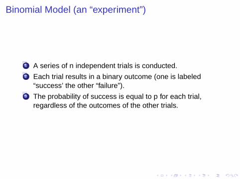
Binomial Random Variable

The number of “successes” in the binomial experiment.

Let Y = # of success in the above model.

Then Y is a binomial random variable with parameters n(sample size) and p (success probability). It is oftendenoted

Y ∼ B(n, p).

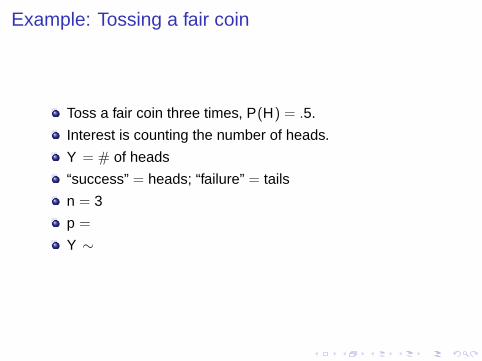
Example: Tossing a fair coin

Toss a fair coin three times, P(H) = .5.

Interest is counting the number of heads.

Y = # of heads

“success” = heads; “failure” = tails

n =

p =

Y ∼

Example: Tossing a fair coin

Toss a fair coin three times, P(H) = .5.

Interest is counting the number of heads.

Y = # of heads

“success” = heads; “failure” = tails

n = 3

p =

Y ∼

Example: Tossing a fair coin

Toss a fair coin three times, P(H) = .5.

Interest is counting the number of heads.

Y = # of heads

“success” = heads; “failure” = tails

n = 3

p = .5

Y ∼

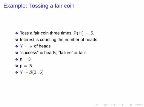
Example: Tossing a fair coin

Toss a fair coin three times, P(H) = .5.

Interest is counting the number of heads.

Y = # of heads

“success” = heads; “failure” = tails

n = 3

p = .5

Y ∼ B(3, .5)

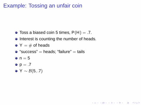
Example: Tossing an unfair coin

Toss a biased coin 5 times, P(H) = .7.

Interest is counting the number of heads.

Y = # of heads

“success” = heads; “failure” = tails

n = 5

p = .7

Y ∼ B(5, .7)

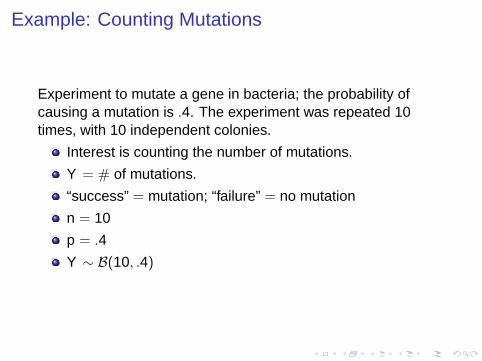
Example: Counting Mutations

Experiment to mutate a gene in bacteria; the probability ofcausing a mutation is .4. The experiment was repeated 10times, with 10 independent colonies.

Interest is counting the number of mutations.

Y = # of mutations.

“success” = mutation; “failure” = no mutation

n = 10

p = .4

Y ∼ B(10, .4)

Computing Probabilities for a Binomial Random Variable.

Board Example

Tossing a biased coin; Y ∼ B(3, .7).

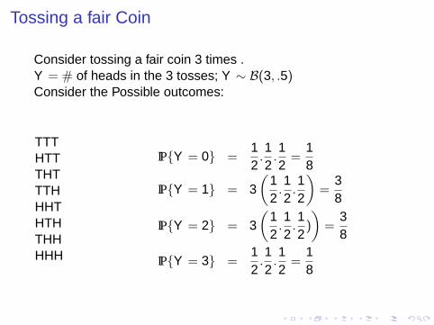
Tossing a fair Coin

Consider tossing a fair coin 3 times .Y = # of heads in the 3 tosses; Y ∼ B(3, .5)Consider the Possible outcomes:

TTTHTTTHTTTHHHTHTHTHHHHH

IP{Y = 0} =12.12.12

=18

IP{Y = 1} = 3(

12.12.12

)=

38

IP{Y = 2} = 3(

12.12.12)

)=

38

IP{Y = 3} =12.12.12

=18

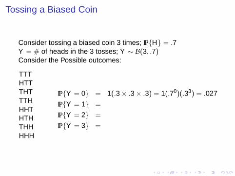
Tossing a Biased Coin

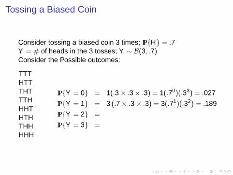
Consider tossing a biased coin 3 times; IP{H} = .7Y = # of heads in the 3 tosses; Y ∼ B(3, .7)Consider the Possible outcomes:

TTTHTTTHTTTHHHTHTHTHHHHH

IP{Y = 0} = 1(.3× .3× .3) = 1(.70)(.33) = .027

IP{Y = 1} =

IP{Y = 2} =

IP{Y = 3} =

Tossing a Biased Coin

Consider tossing a biased coin 3 times; IP{H} = .7Y = # of heads in the 3 tosses; Y ∼ B(3, .7)Consider the Possible outcomes:

TTTHTTTHTTTHHHTHTHTHHHHH

IP{Y = 0} = 1(.3× .3× .3) = 1(.70)(.33) = .027

IP{Y = 1} = 3 (.7× .3× .3) = 3(.71)(.32) = .189

IP{Y = 2} =

IP{Y = 3} =

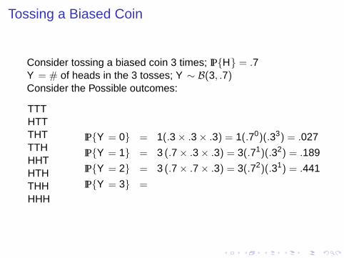
Tossing a Biased Coin

Consider tossing a biased coin 3 times; IP{H} = .7Y = # of heads in the 3 tosses; Y ∼ B(3, .7)Consider the Possible outcomes:

TTTHTTTHTTTHHHTHTHTHHHHH

IP{Y = 0} = 1(.3× .3× .3) = 1(.70)(.33) = .027

IP{Y = 1} = 3 (.7× .3× .3) = 3(.71)(.32) = .189

IP{Y = 2} = 3 (.7× .7× .3) = 3(.72)(.31) = .441

IP{Y = 3} =

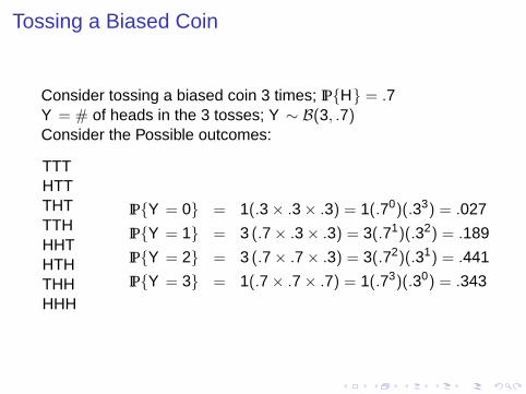
Tossing a Biased Coin

Consider tossing a biased coin 3 times; IP{H} = .7Y = # of heads in the 3 tosses; Y ∼ B(3, .7)Consider the Possible outcomes:

TTTHTTTHTTTHHHTHTHTHHHHH

IP{Y = 0} = 1(.3× .3× .3) = 1(.70)(.33) = .027

IP{Y = 1} = 3 (.7× .3× .3) = 3(.71)(.32) = .189

IP{Y = 2} = 3 (.7× .7× .3) = 3(.72)(.31) = .441

IP{Y = 3} = 1(.7× .7× .7) = 1(.73)(.30) = .343

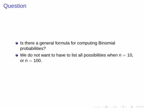
Question

Is there a general formula for computing Binomialprobabilities?

We do not want to have to list all possibilities when n = 10,or n = 100.

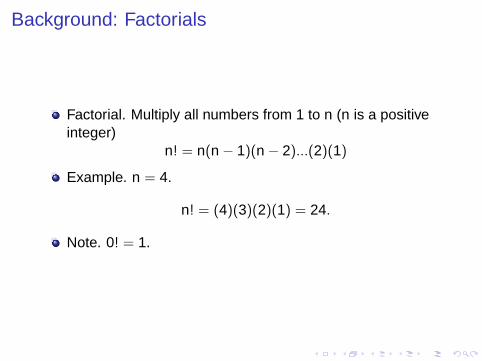
Background: Factorials

Factorial. Multiply all numbers from 1 to n (n is a positiveinteger)

n! = n(n − 1)(n − 2)...(2)(1)

Example. n = 4.

n! = (4)(3)(2)(1) = 24.

Note. 0! = 1.

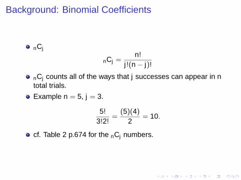
Background: Binomial Coefficients

nCj

nCj =n!

j!(n − j)!

nCj counts all of the ways that j successes can appear in ntotal trials.

Example n = 5, j = 3.

5!

3!2!=

(5)(4)

2= 10.

cf. Table 2 p.674 for the nCj numbers.

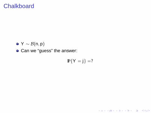
Chalkboard

Y ∼ B(n, p)

Can we “guess” the answer:

IP{Y = j} =?

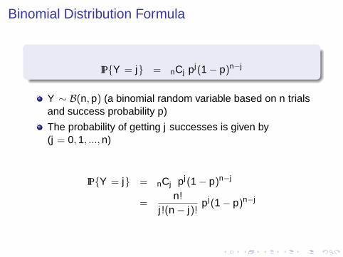
Binomial Distribution Formula

IP{Y = j} = nCj pj(1− p)n−j

Y ∼ B(n, p) (a binomial random variable based on n trialsand success probability p)

The probability of getting j successes is given by(j = 0, 1, ..., n)

IP{Y = j} = nCj pj(1− p)n−j

=n!

j!(n − j)!pj(1− p)n−j

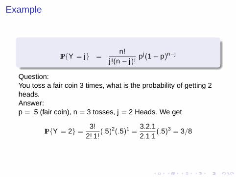
Example

IP{Y = j} =n!

j!(n − j)!pj(1− p)n−j

Question:You toss a fair coin 3 times, what is the probability of getting 2heads.Answer:p = .5 (fair coin), n = 3 tosses, j = 2 Heads. We get

IP{Y = 2} =3!

2! 1!(.5)2(.5)1 =

3.2.12.1 1

(.5)3 = 3/8

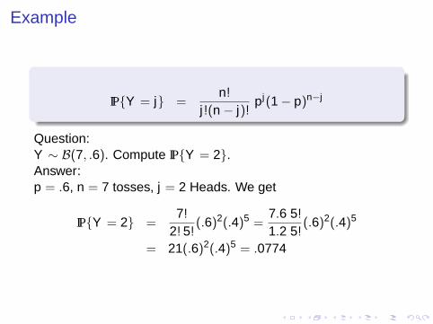
Example

IP{Y = j} =n!

j!(n − j)!pj(1− p)n−j

Question:Y ∼ B(7, .6). Compute IP{Y = 2}.Answer:p = .6, n = 7 tosses, j = 2 Heads. We get

IP{Y = 2} =7!

2! 5!(.6)2(.4)5 =

7.6 5!

1.2 5!(.6)2(.4)5

= 21(.6)2(.4)5 = .0774

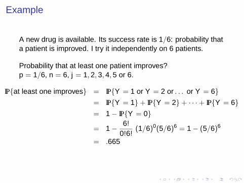
Example

A new drug is available. Its success rate is 1/6: probability thata patient is improved. I try it independently on 6 patients.

Probability that at least one patient improves?p = 1/6, n = 6, j = 1, 2, 3, 4, 5 or 6.

IP{at least one improves} = IP{Y = 1 or Y = 2 or . . . or Y = 6}= IP{Y = 1}+ IP{Y = 2}+ · · ·+ IP{Y = 6}= 1− IP{Y = 0}

= 1− 6!

0!6!(1/6)0(5/6)6 = 1− (5/6)6

= .665

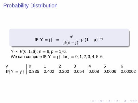
Probability Distribution

IP{Y = j} =n!

j!(n − j)!pj(1− p)n−j

Y ∼ B(6, 1/6); n = 6, p = 1/6.We can compute IP{Y = j}, for j = 0, 1, 2, 3, 4, 5, 6.

y 0 1 2 3 4 5 6IP{Y = y} 0.335 0.402 0.200 0.054 0.008 0.0006 0.00002

Mean, Variance, and Standard Deviation for BinomialRandom Variables

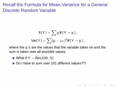
Recall the Formula for Mean,Variance for a GeneralDiscrete Random Variable

E(Y ) =∑

yi IP{Y = yi} ,

Var(Y ) =∑

(yi − µY )2IP{Y = yi} ,

where the yi ’s are the values that the variable takes on and thesum is taken over all possible values.

What if Y ∼ Bin(100, .5)

Do I have to sum over 101 different values?!?

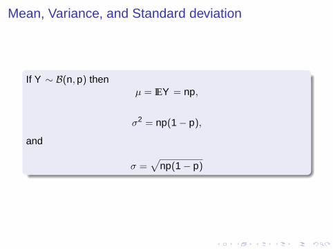
Mean, Variance, and Standard deviation

If Y ∼ B(n, p) thenµ = IEY = np,

σ2 = np(1− p),

and

σ =√

np(1− p)

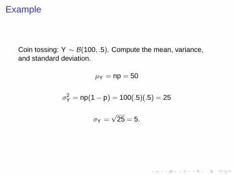
Example

Coin tossing: Y ∼ B(100, .5). Compute the mean, variance,and standard deviation.

µY = np = 50

σ2Y = np(1− p) = 100(.5)(.5) = 25

σY =√

25 = 5.

The assumptions for the binomial model

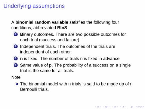
Underlying assumptions

A binomial random variable satisfies the following fourconditions, abbreviated BInS .

1 Binary outcomes. There are two possible outcomes foreach trial (success and failure).

2 Independent trials. The outcomes of the trials areindependent of each other.

3 n is fixed. The number of trials n is fixed in advance.4 Same value of p. The probability of a success on a single

trial is the same for all trials.

Note

The binomial model with n trials is said to be made up of nBernoulli trials.

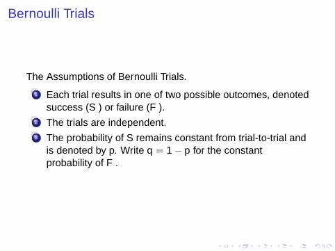
Bernoulli Trials

The Assumptions of Bernoulli Trials.

1 Each trial results in one of two possible outcomes, denotedsuccess (S ) or failure (F ).

2 The trials are independent.3 The probability of S remains constant from trial-to-trial and

is denoted by p. Write q = 1− p for the constantprobability of F .

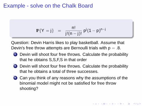
Example - solve on the Chalk Board

IP{Y = j} =n!

j!(n − j)!pj(1− p)n−j

Question: Devin Harris likes to play basketball. Assume thatDevin’s free throw attempts are Bernoulli trials with p = .8.

1 Devin will shoot four free throws. Calculate the probabilitythat he obtains S,S,F,S in that order

2 Devin will shoot four free throws. Calculate the probabilitythat he obtains a total of three successes.

3 Can you think of any reasons why the assumptions of thebinomial model might not be satisfied for free throwshooting?

Examples for You

Example 3.45, p.106

Examples 3.47, 3.48 p.108-109

Example 3.49 p.109

Example 3.50 p.110 (when assumptions might be violated).