The Big Thaw: Simulating Greenland's Future - Peoplepeople.sc.fsu.edu/~jburkardt/presentations/climate_2011_fsu.pdf · The Big Thaw: Simulating Greenland’s Future John Burkardt

The Big Thaw: Simulating Greenland’s Future

John BurkardtGraduate Student Seminar

Department of Scientific ComputingFlorida State University

..........http://people.sc.fsu.edu/∼jburkardt/presentations/...

climate 2011 fsu.pdf

3pm, 08 April 2011

1 / 66


Introduction

The Big Picture

Mathematical Modeling

The Finite Volume Model

Moving to Finite Elements

Conclusion

2 / 66

Introduction

In recent decades, a slight but steady increase in averageworld-wide temperature was noticed. This was attributed to theeffects of industrialization, reduction in tree cover, increasedburning of fossil fuels, the role of carbon dioxide in absorbinggreater amounts of solar energy.

Even if the mechanisms are still just plausible hypotheses, theslight but steady rise in temperature has continued. It is natural toask the straightforward question:

Is anything important likely to happen to the Earth if thetemperature continues to increase?

3 / 66

Introduction

The question being asked is a modeling question. In otherwords, we are not asking if the temperature is rising a little eachyear, or by how much.

We are assuming a certain yearly rise in temperature, and asking ifwe can produce a plausible climate model which can exhibit theexpected results.

Obviously, we would be interested in checking several differentestimates for the increase, and if we model the climate, we’d likethe actual yearly rise to vary in some statistical way about theestimated average rise.

Modeling the global climate is really hard. While we understandthe properties of air, ocean, land and sunshine in general, we havelimited understanding of common things such as clouds and of big,slowly moving things (glaciers and ice sheets).

4 / 66

Introduction: Climate is Complicated!

We know that many glaciers around the world have retreated oreven melted away. That suggests that we might need to beconcerned about the really enormous ice sheets in Greenland andAntarctica.

It would be easy to make a first guess that, if the globaltemperature is rising, then these sheets also will melt away.

But these easy guesses are worthless, because the Earth’s climateis a strangely complicated thing. Initial investigations have alreadysuggested that, at least in the beginning, the overall warming ofthe Earth would result in increased snowfall in Greenland, so thatthe ice sheet would get thicker.

Which also means that if we had chosen to look at the thickness ofGreenland’s ice as an indicator of the climate, we’d wronglyconclude that things are getting better!

5 / 66

Introduction: Don’t Argue, Predict!

The important thing to do, then, is to take practical, accurate,scientific models, implement them as well as we can, and use themto make predictions for the near and long-term future.

We can then try to answer the question of whether climatemodeling is believable by comparing the short-term predictions tothe actual observed behavior over the next decade.

If these predictions are reasonably accurate, then the longer-termpredictions (whatever they may be) will be more acceptable.

Failures of prediction are also useful in helping to improve themodel (and to restart the prediction process.)

6 / 66

Introduction: Calving from an Ice Sheet

7 / 66

Introduction

It’s hard to say whether the melting of a single glacier hashappened because the climate has changed, or that this meltingcould, in turn, have an effect on the climate.

But an ice sheet can be the size of a small continent (Greenlandand Antarctica, in particular); the ice can be two miles thick. TheGreenland ice alone could raise the ocean 20 feet.

In other words, changes to the Greenland ice sheet are likely torepresent important climate effects, and to cause further changes.

The ice in Greenland accumulates and moves slowly towards theocean. The movement is resisted by a strong frictional force wherethe ice sheet rests on bedrock. This is usually a “dry” contact, butin some places, geothermal heat overcomes the enormous pressure,and the ice sheet slides quickly over a wet contact.

8 / 66

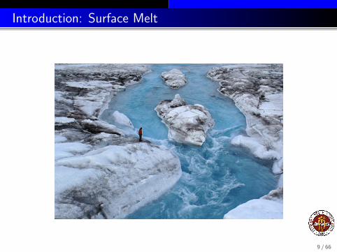
Introduction: Surface Melt

9 / 66

Introduction: Simulating the Ice Sheets

The goal of a simulation is to take some model of the earth’stemperature profile and to simulate the resulting climate over aperiod of 100 years.

There are already computer programs available which attempt thistask, but in order to make any computations, they’ve had to makenumerous short cuts and estimates, and to simply admit thatcertain parts of the model are not well understood.

Because climate is so complex, many climate models areconstructed out of separate programs, each of which models aparticular feature. Each program outputs its current status atregular points, and can accept input from other programs or elseuse “canned” or approximate data in a stand-alone run.

Climate programs have a limited understanding of the ice sheets ofGreenland and Antarctica.

10 / 66

Introduction: CESM

For example, there is a system called CESM or the CommunityEarth System Model. It comprises five physical models,implemented as computer programs by separate teams, including:

ATM, atmosphere (clouds, vapor, radiation, pollutants);

LND, land surface;

OCN, ocean;

ICE, sea ice;

GLC, ice sheets (Greenland/Antarctica);

The ice sheet model is a relatively new addition to CESM.

http://www.cesm.ucar.edu

11 / 66

Introduction: New Ice Sheet Model

Since 1990, the Intergovernmental Panel on Climate Change orIPCC, has issued a report every five to seven years, summarizingthe state of knowledge and proposing areas where a betterunderstanding is needed.

The Fourth Report was issued in 2007, and declared that currentclimate models were not able to properly analyze thecontinental-sized ice sheets covering Greenland and Antarctica.

The panel complained of:

insufficient data of topography, snow fall, ice depth, velocity;

low accuracy models of ice sheet physics;

insufficient resolution in time and space;

computer programs unable to interface with programsmodeling the ocean and atmosphere;

12 / 66

Introduction: New Ice Sheet Model

One of the most controversial topics in climate modelinginvolves predictions of the future level of the ocean.

Because the ice sheets lock up an enormous amount of water, acredible prediction of changes in sea level must be based onconfidence in the predictions of the ice sheets.

The 2007 panel refused to make a prediction on sea level changesbecause of the uncertainty over ice sheet behavior.

The Fifth Report will be issued in 2014, and the panel demandedthat by that time researchers must produce credible, detailed icesheet data needed to predict ocean levels.

http://www.ipcc.ch/

13 / 66

Introduction: How CESM Changes are Made and Approved

CESM is one of about 12 separate computer models of the earth’sclimate developed by various research groups.

CESM is led by researchers at NCAR, the National Center forAtmospheric Research, in Boulder, Colorado, which has a longhistory of work in weather and climate. However, the componentprograms have come from a variety of universities andorganizations, and are supported and developed by somewhatautonomous teams of scientists.

Significant changes to a CESM component program must beapproved by a larger group before they are accepted into a newrelease of that program.

14 / 66

Introduction: Teams

Several teams have assembled to make improvements toGlimmer-CISM, the Community Ice Sheet Model that CESM usesto model Greenland and Antarctica.

Bill Lipscomb, at Los Alamos National Laboratory, is in overallcharge of an effort funded by the Department of Energy. He has ateam at LANL trying to implement more realistic physical modelsfor the ice sheet; Kate Evans, at Oak Ridge National Laboratory, isdirecting a team looking at improving the solver. There is anotherteam at Lawrence Berkeley Lab, under Esmond Ng.

Bill Lipscomb decided to seek research and programming supportfrom Max Gunzburger (FSU) and Lili Ju (SC), who have formed asmall group consisting of postdoctoral students Mauro Perego, TaoCui, and Wei Leng, slightly assisted by me.

15 / 66

Introduction: GLIMMER

The Glimmer program has been used for over thirty years tomodel ice sheets.

That’s good, because the program has accumulated a lot ofknowledge; but it also means that the program still has manyfeatures that are becoming brittle and out of date.

It is a large program, written in FORTRAN, uses a rectangularequally-spaced grid, a relatively simple physics model, and aniterative solver that can be slow to converge.

Needless to say, Glimmer is not a parallel code.

16 / 66

Introduction: GLIMMER

Because of its history and widespread acceptance amongice-sheet modelers, Glimmer was chosen to join the CESM systemas the ”Community Ice Sheet Model”. The version of Glimmerbeing adapted for this purpose is now called Glimmer-CISM.

We are working with researchers at Oak Ridge, who are trying toreplace the old solver with a more sophisticated iteration, and toparallelize the solution procedure, while still (currently) working ona rectangular grid.

https://glimmer-cism.berlios.de/

17 / 66

Introduction: MPAS

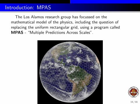
The Los Alamos research group has focussed on themathematical model of the physics, including the question ofreplacing the uniform rectangular grid, using a program calledMPAS - “Multiple Predictions Across Scales”.

18 / 66

Introduction: MPAS

The MPAS program is very general; it is designed to work witha sophisticated polygonal grid over all or some of the Earth’ssurface. The user places some variables at the centers of cells;fluxes are associated with the interfaces between cells and certainother quantities are assigned at the vertices of the cells.Discretized versions of the state equations are used to update thevalues over time in a way that obeys conservation laws.

The Los Alamos researchers are especially interested in formulatingthe physical equations of the ice sheet model in a way that MPAScan handle, and to generate a CVT-style mesh over Greenland thathas high resolution in areas where the ice sheet is moving fast.

http://mpas.sourceforge.net

19 / 66


Introduction

The Big Picture




Conclusion

20 / 66

BIG PICTURE: How to Find Greenland

Greenland has an area of about 2,000,000 km2.

Ice covers 85% of the surface, to a maximum depth of 3 km.

21 / 66

BIG PICTURE: Greenland and Climate

The purpose of the investigation is to “plug” Greenland intoprograms that model global climate.

The primary effects that Greenland exerts on the external climate(ocean and atmosphere) include:

the temperature of the surface of the ice sheet;

the reflectance of solar radiation from surfaces covered by ice;

the rate at which ice and meltwater flows into the ocean;

where the land-based ice sheet extends into the ocean, theocean and atmosphere become ”decoupled”;

The external climate’s effect on Greenland can be summarized by

solar radiation, moderated by cloud cover;

heat transfer with the atmosphere;

snowfall, which builds the ice sheet.

a geothermal flux through the bottom of the ice sheet.22 / 66

BIG PICTURE: State Variables

The behavior of the ice sheet can be understood in terms of thefollowing state variables:

the temperature T (x , y , z);

the pressure P(x , y , z);

the velocity ~V (x , y , z);

the ice thickness H(x , y);

the elevation, or position of the top of the ice sheet, Q(x , y).

We assume that density is essentially constant.

Because we are modeling such a large region, we do not try tostudy localized features such as cracks and faults in the ice.

23 / 66

BIG PICTURE: Current Resolution 5km x 5km

Currentsimulations produce valuesof the state variables on aspatial grid that is horizontallyuniform (5km x 5km). Thiscorresponds to a rectangulargrid of 301 (East to West) by561 (North to South) cells by11 layers → 1.5 million nodes.

The needed resolution is 1kmx 1km, at least in areas of highice-sheet velocity; this couldbe 25 times as many nodes.

24 / 66

BIG PICTURE: Rectangular Grid

When we ask for a resolution of 1km x 1km, we are really justasking for ”five times” the linear resolution of the 5km x 5km.There are vast parts of Greenland where nothing is happening, theice is not moving, and no finer resolution is ever needed. But wedo need to follow the areas of rapid ice movement carefully.

The current version of Glimmer-CISM uses a uniform rectangulargrid. That means that to see a single point at high resolutionrequires using that same high resolution everywhere.

Since Greenland is not a rectangle, it means that many grid cellsare placed in the ocean, where they do nothing (but cost usstorage and time).

Greenland’s coast is not straight, but it will be modeled as thoughit were constructed out of horizontal and vertical lines.

25 / 66

BIG PICTURE: Ice Thickness

26 / 66

BIG PICTURE: Normalizing the Ice Thickness

In the vertical direction, the grid might use 11 proportionallyspaced levels from bedrock to ice surface;

In other versions of the ice sheet model (but not ours!) the verticaldirection is rescaled to a variable σ in the range [0,1].

This seems to make life easier, since the top of the ice is nowalways at σ = 1, but since the ice thickness varies over space andtime, this means that the (x , y , σ) grid is not orthogonal.Equations with spatial derivatives suddenly inherit geometriccorrections that look like fictitious forces...so we don’t do this!

27 / 66

BIG PICTURE: Long Time Interval

To perform simulations as desired, the model must be able tocompute data over a time span of 100 years, using a time step thatmay be on the order of 1 year.

Despite the fact that we are dealing with ice, a time step of a yearmeans we must worry about the CFL (Courant-Friedrichs-Levy)condition, which essentially says that a flow particle mustn’t crossmore than one spatial cell in a time step.

∆t ≤ C ∗ u ∗∆x

The velocity of the ice sheet varies from between 1 to 400 m/year;the current grid has a resolution of about 5 km, while the goal isto provide a resolution of 1 km.

This applies for temperature and thickness, but, surprisingly, notfor velocity, because of a quasi-static assumption!

28 / 66

BIG PICTURE: Tight Accuracy Requirement

The physical system satisfies conservation of energy and mass.

The equations used in the model should satisfy these conditionsexactly, that is, to within machine roundoff.

In particular, the mass of ice at the beginning, plus all snowfall,minus all calving, must equal the mass at the end of the century,to 16 decimal places, with a similar requirement on energy.

29 / 66


Introduction

The Big Picture




Conclusion

30 / 66

MODEL: The Thickness Equation

The thickness H(x , y) of the ice changes with snowfall andmotion of the ice sheet:

∂H

∂t= Hflux −∇ ·

∫z

[uv

]dz

Hflux is the flux due to snowfall;

Assuming the ice always flows outward, the boundary condition forthickness can be taken as a homogeneous Neumann condition.

31 / 66

MODEL: The Temperature Equation

The evolution equation for temperature T :

ρc∂T

∂t=

∂

∂z(κ∂T

∂z)− ρc(~u · ∇T ) + 2ε̇ :: σ

c is the heat capacity;

ρ the (constant) density;

κ is the thermal conductance;

ε̇ is the strain rate tensor;

σ is the stress tensor.

32 / 66

MODEL: The Temperature Boundary Conditions

Ice at the surface is assigned the mean annual surfacetemperature.

Ice at the bedrock boundary is subject to geothermal flux G andheat generated by sliding friction:

−k∇T · ~n = G +~t · ~u

33 / 66

MODEL: Stokes Equations for Velocity

The ice sheet can be regarded as a very viscous liquid with a tinyReynolds number. A quasi-static assumption means that we canalso drop the time derivative. What follows is a form of Stokesequation for velocity ~U with a variable viscosity:

−∇ · B(T ) |ε̇e |1−n

n (∇U + (∇U)′))/2 +∇P =

00−ρg

∇ · U = 0

ρ is the density, g the unit gravitational force;

|ε̇e | is the norm of the strain rate tensor;

n ≈ 3;

B(T ) is a constitutive coefficient.

34 / 66

MODEL: Simplified Velocity Equations

Because the ice flow tends to be predominantly in the horizontalplane, it is possible to simply the velocity state equations evenfurther. Simplified models produce smaller sets of equations thatcan be solved faster.

Three levels of simplification include:

The 1st order model: simplifying the momentum balance inthe Z direction, and incorporating this assumption into the Xand Y force balance equations;

“Shallow Ice Equations”: assuming that pressure is strictly afunction of height, and has the formP(x , y , z) = ρg(Q(x , y)− z) where Q(x , y) is the position ofthe top of the ice sheet; it is suitable for slow-sliding regions;

“Shallow Shelf Equations” are a simplification of the 1st ordermodel suitable for fast-sliding regions.

35 / 66


Introduction

The Big Picture




Conclusion

36 / 66

Finite Volumes: A Staggered Grid

The horizontal domain is approximated by a pair of grids,sometimes referred to as the (i , j) and (r , s) grids.

Horizontal velocities U and V are assigned to (r , s) nodes.

Vertical velocities W , ice thickness H, and temperature T , areassigned to (i , j) nodes.

Copies of these 2D grids are generated for each ice sheet layer.

37 / 66

Finite Volumes: Gradients

Gradients of (r , s) objects are assigned to (i , j) nodes:

(∂u

∂x)i ,j ≈

ur ,s + ur ,s−1 − ur−1,s − ur−1,s−1

2∆x

A conservation law, written using this kind of scheme for gradients,will correctly conserve the quantity of interest.

38 / 66

Finite Volume: Forming Discrete System

Using the staggered meshes to form approximations toderivatives, and a constant stepsize in time, it is possible todiscretize the equations for temperature, ice thickness, and velocity.

Starting from some initial condition, the solution is advanced bytimesteps.

Because the number of variables is so large, and the system ofequations includes nonlinearities, a direct solution is notattempted. Instead, an iterative scheme is employed. At each stepof the nonlinear iteration, several linear systems must be solved.Each of these systems is also solved iteratively, using the SLAPsparse linear algebra package.

http://www.netlib.org/slap

39 / 66

Finite Volume: Solving Discrete System

The system size is reduced by uncoupling the state variableequations, and by uncoupling the ice sheet layers.

In particular, the iteration proceeds as follows:

update the horizontal velocities using the first order equations;

back out the vertical velocities, to get ~U(x , y , z);

for each point on the ice sheet bottom layer, integrate the icethickness equation to update H(x , y);

by ignoring the effects of horizontal dissipation, integrate thetemperature equation from bottom layer to top to getT (x , y , z);

Although information seems to flow only upwards, couplingcoefficients relate adjacent ice sheet layers, so information alsotravels downwards as the iteration proceeds.

40 / 66

Finite Volume: Parallelism

For each subsystem being solved, the variables are laid out on ahorizontal mesh.

To evaluate the equations defined at a node, it is typicallynecessary to access data at neighbor nodes to the east, west, northand south, as well as the lower and upper layers.

A parallel implementation which divides up the rectangular gridinto subrectangles must enable each subrectangle to obtain someinformation from adjacent subrectangles. This is done byaugmenting each partial grid with a layer of ”ghost cells” or ”halocells”, which are available as information, and do not need to beupdated.

41 / 66

Finite Volume: Ghost Cells

42 / 66


Introduction

The Big Picture




Conclusion

43 / 66

Finite Elements: Advantages

The contribution of our group has been to implement a revisedtreatment of the calculation using a grid adapted to the geometryand known ice behavior (Lili Ju), and a reformulation of the stateequations using finite elements (Mauro Perego).

By abandoning the rectangular grid:

we no longer waste time modeling bits of the ocean;

we can more accurately follow the coastline of Greenland, andany other geometric objects;

we can provide a refined mesh in areas of Greenland where theice sheet velocity is known to be high;

we can use a grid that smoothly interfaces with gridsemployed by global climate modeling programs, so that datafrom one program can be used by the other.

44 / 66

Finite Elements: Observed Ice Sheet Velocity

45 / 66

Finite Elements: a Sample Grid Adapted to Velocity

46 / 66

Finite Elements: Detail of Coastline Grid

47 / 66

Finite Elements: Using Triangular Prisms for 3D Elements

Starting from a 2D triangular grid that meshes a “flattened”version of Greenland, we can build layers in the z direction byconstructing triangular prisms.

For our model, which involves 11 layers from bedrock to surface,we essentially form a stack of 10 such prisms on every triangle ofthe original 2D mesh.

48 / 66

Finite Elements: 3 Tetrahedrons in each Prism

In 3D, the tetrahedron plays the role of fundamental finiteelement shape. So once we have set up our prisms, we decomposeeach into 3 tetrahedrons, inside of which we can do our usual finiteelement computations.

49 / 66

Finite Elements: Example of a Triangular Prism Grid

This is not the grid for an ice sheet, but it suggests the layerednature of the triangular prism grid.

50 / 66

Finite Elements: Example of a Triangular Prism Grid

All the state equations can be discretized using the same mesh.

The parallel assembly of the system matrix does not require anycommunication between processors at all.

The parallel solution of the linear systems arising in the nonlineariteration at each time step only requires the use of an appropriatelibrary solver.

In fact, the solution of the entire nonlinear system can also bedone in parallel, using an off-the-shelf library solver.

We use Sandia National Laboratory’s Trilinos package.

http://trilinos.sandia.gov/

51 / 66

Finite Elements: Trilinos NOX Nonlinear Solver

NOX is an object-oriented C++ library for large nonlinear systems.It implements Newton-based globalization techniques including linesearch and trust region algortihms. NOX defines interfaces to usercodes through the abstract group and vector pure virtual classes.

The user can supply the underlying linear algebra solver needed byTrilinos to carry out the iterations involved in solving the nonlinearsystem.

To improve performance, the user can supply preconditioning orjacobian information.

http://trilinos.sandia.gov/packages/nox/

52 / 66

Finite Elements: Trilinos EPETRA Parallel Linear Algebra

Instead of supplying the linear algebra solver, the user can takeadvantage of the Trilinos’s Epetra package. With Epetra the useronly needs to evaluate the residual equation F (x) = 0 for a given x .

Epetra contains classes for distributed sparse and dense matricesand vectors; It provides a flexible and powerful data redistributioncapability for load balancing and scalability of linear algebraalgorithms without the user needing any special knowledge aboutdistributed object.

Epetra provides a parallel machine interface that allows users towrite generate parallel functionality without specifically using anyparticular parallel library.

http://trilinos.sandia.gov/packages/epetra/

53 / 66

Finite Elements: LIFEV Finite Element Library

To increase the order of approximation of a finite difference orfinite volume code can require an extensive rewrite.

For a finite element code, the order of approximation and even theform of the equations are easily changed in a way that does notobviously affect the main user code. Instead, these choices areimplemented in separate code.

LifeV is a C++ package for finite element calculations such asthose involving fluids, heat transfer, structures, porous media. Itmakes extensive use of the modern features of C++, allowing adeveloper to rapidly model a physical system.

Mauro Perego is a developer of the LifeV package, and has beenable to transfer the ice sheet model to this framework and solvebenchmark problems with it.

https://sites.google.com/site/lifevproject54 / 66


Introduction

The Big Picture




Conclusion

55 / 66

Conclusion: A Better Grid

By dropping the uniform rectangular grid and moving to anadaptive mesh:

we reduce the number of wasted cells;

we can better conform to the geometry of the region;

we can choose a weighting function (such as observed icevelocity) to vary the fineness of the mesh;

we can refine the mesh near the coasts for better interactionwith other simulation packages.

This allows us to achieve the desired 1 km x 1km resolution inareas of high ice sheet velocity.

56 / 66

Conclusion: Grid interfaces

The grid is flexible, and can be refined at the coastline so it canexchange more detailed information with a separate programmodeling the ocean.

57 / 66

Conclusion: Using Finite Elements

By formulating the problem using finite elements:

we are able to use the adaptive mesh;

increasing the approximation power only requires changing aparameter;

approximated state variables can be evaluated anywhere;

the nonlinear solution can be handed off to an external library;

the parallelism can be handed off to an external library.

58 / 66

Conclusion: Arolla Glacier Test Case

59 / 66

Conclusion: Sample Greenland Calculations

Using the finite element model that Mauro Perego has developed,we are able to run mathematical models of increasing accuracy(Shallow Ice, Shallow Shelf, First Order, L1L0) on grids of thedesired resolution.

Mauro used 10 layers, for a total of 3.9 million tetrahedra and 1.4million unknowns. The temperature field is given and rangesbetween 250 to 273 K. No slip boundary conditions were alwaysused at the bedrock, because sliding data was not available.

60 / 66

Conclusion: SIA Model versus First Order

61 / 66

Conclusion: Velocity Vector Closeup

62 / 66

Conclusion: Using TRILINOS Package

By using TRILINOS and EPETRA for solving F (X ) = 0 andA ∗ x = b:

we are no longer responsible for the housekeeping detailsrequired when implementing a parallel code;

we guarantee good parallel performance on a wide range ofconfigurations

we have access to a variety of high-quality linear and nonlinearsolvers with a uniform interface.

63 / 66

Conclusion

Our challenges include:

implementing the temperature and thickness equations infinite element form (right now, we are only doing thevelocities this way);

converting the routines in LifeV from C++ to FORTRAN90,because the climate community insists on a uniform language;

matching the very tight tolerances (∼ machine precision) onconservation of mass and energy over the 100 year simulationcycles;

finishing the process of verification, documentation, andpublication before the end of 2012, after which no new inputwill be accepted for the Intergovernmental Panel on ClimateChange (IPCC) Assessment Report 5 to be published in 2014.

64 / 66

Conclusion: Colleagues and Reference

FSU/SC: Max Gunzburger, Lili Ju, Tao Cui, Wei Leng, MauroPerego (gridding and finite elements);

NYU: Jean-Francois Lemieux (solver);

Oak Ridge; Kate Evans, Jeff Nichols, Pat Worley;

Los Alamos; Bill Lipscomb, Steve Price, Todd Ringler, XylerAsay-Davis, Dana Knoll;

Sandia: Andy Salinger (Trilinos);

Mauro Perego, Max Gunzburger, John Burkardt,Implementation and comparison of linear and quadratic finiteelement methods for higher-order ice-sheet models,submitted, Journal of Glaciology.

65 / 66

Conclusion: Follow Up Seminar Begins at 5:30++

The Mellow Mushroom Institute

66 / 66

Documents

The Big Thaw: Simulating Greenland's Future - Peoplepeople.sc.fsu.edu/~jburkardt/presentations/climate_2011_fsu.pdf · The Big Thaw: Simulating Greenland’s Future John Burkardt