The B.E. Journal of Theoretical Economicsmath.uchicago.edu/~shmuel/Network-course-readings...Fudenberg (1993, 1995) were among the rst to examine the collective out-come of individual

The B.E. Journal of TheoreticalEconomics

TopicsVolume 10, Issue 1 2010 Article 36

Social Learning in Social Networks

PJ Lamberson∗

∗Massachusetts Institute of Technology, [email protected]

Recommended CitationPJ Lamberson (2010) “Social Learning in Social Networks,” The B.E. Journal of Theoretical Eco-nomics: Vol. 10: Iss. 1 (Topics), Article 36.Available at: http://www.bepress.com/bejte/vol10/iss1/art36

Copyright c©2010 The Berkeley Electronic Press. All rights reserved.

Social Learning in Social Networks∗

PJ Lamberson

Abstract

This paper analyzes a model of social learning in a social network. Agents decide whetheror not to adopt a new technology with unknown payoffs based on their prior beliefs and the ex-periences of their neighbors in the network. Using a mean-field approximation, we prove thatthe diffusion process always has at least one stable equilibrium, and we examine the dependenceof the set of equilibria on the model parameters and the structure of the network. In particular,we show how first and second order stochastic dominance shifts in the degree distribution of thenetwork impact diffusion. We find that the relationship between equilibrium diffusion levels andnetwork structure depends on the distribution of payoffs to adoption and the distribution of agents’prior beliefs regarding those payoffs, and we derive the precise conditions characterizing thoserelationships. For example, in contrast to contagion models of diffusion, we find that a first orderstochastic dominance shift in the degree distribution can either increase or decrease equilibriumdiffusion levels depending on the relationship between agents’ prior beliefs and the payoffs toadoption. Surprisingly, adding more links can decrease diffusion even when payoffs from the newtechnology exceed those of the status quo in expectation.

KEYWORDS: social networks, learning, diffusion, mean-field analysis, stochastic dominance

∗The author wishes to thank Georgia Kernell, Federico Echenique, and an anonymous reviewerfor their helpful comments on earlier drafts of this article.

1 Introduction

When choosing whether or not to adopt a new technology, people often relyon information outside of their personal experience to make their decision.One potential source of information is other individuals who have alreadytried the technology. If the information from previous adopters is sufficientlypositive, an initially skeptical individual may be convinced to adopt, makingthem a potential source of information for others in the future. Collectively, thepopulation learns about the value of the new technology as it spreads throughthe market. This mechanism of social learning is a simple but compellingexplanation for technology diffusion.

In seeking information from previous adopters, individuals most likelyturn to their friends and acquaintances – in other words neighbors in their socialnetwork (Jackson, 2008). In this paper we analyze a model of social learning inwhich agents are embedded in a social network that dictates who interacts withwhom. Each agent in the model employs a boundedly rational decision-makingrule to determine whether or not to adopt a new technology. Specifically,agents combine information on the payoffs received by their adopting neighborswith their prior beliefs using Bayes’ rule, and they adopt the technology iftheir resulting posterior beliefs regarding the value of the technology exceedthe known payoff of the status quo. Agents in the model may also discontinueusing the technology if payoffs observed later cause them to revise their beliefsabout the technology’s benefits. In contrast to fully rational agents, theseagents ignore some information available to them, such as the implicationsthat a neighbors’ adoption decision has regarding the payoffs received by thatneighbor’s neighbors. These limitations reflect our belief that the calculationsrequired of fully rational agents – which include not only reasoning about ourneighbors’ actions, but also reasoning about their reasoning about our actionsand so on – are more complex then what actual people can, or are willing to,perform (Simon, 1955).

To analyze the resulting diffusion we employ an approximation tech-nique from statistical physics known as a mean-field approximation (Chandler,1987), which has proven useful for studying network dynamics in several con-texts (Newman, Moore, and Watts, 2000, Pastor-Satorras and Vespignani,2001a,b, Jackson and Yariv, 2005, 2007, Jackson and Rogers, 2007, Lopez-Pintado, 2008, Lamberson, 2009). We prove that this approximation to thesocial learning process always has at least one stable equilibrium. In generalthere may be multiple stable equilibria. We derive conditions that guaranteea unique stable equilibrium for “costly” technologies, i.e. those with meanpayoff less than that of the status quo, and explain why non-costly technolo-

1

Lamberson: Social Learning in Social Networks

Published by The Berkeley Electronic Press, 2010

gies are more likely to give rise to multiple equilibria. We then proceed toanalyze how equilibrium levels of diffusion depend on the parameters of themodel, specifically the distribution of payoffs to adoption and the distributionof agents’ prior beliefs regarding those payoffs. Some of these relationships arethe same as in models without network structure: higher payoffs and higherpriors result in greater diffusion. However, the effects of changing the varianceof the payoff distribution or the variance of the distribution of priors dependson the network.

The chief advantage of this model in comparison with previous studiesof social learning is the inclusion of potentially complex network structuresthat govern agent interactions. We prove that networks matter for diffusion:changes in network structure cause predictable changes in diffusion levels. Theeffect of network structure on diffusion depends in subtle ways on the relation-ship between the costs or benefits of the new technology and agents’ priorbeliefs about those costs or benefits. Specifically, we consider the effects oftwo types of changes in the network: first and second order stochastic shiftsin the degree distribution. Intuition might suggest that adding more linksto the network (i.e. a first order stochastic shift in the degree distribution)would increase the diffusion of beneficial technologies and decrease diffusionfor those that are costly. We confirm this intuition in some cases, but showthat the opposite is true in others. When the agents’ prior beliefs are suffi-ciently positive, adding links to the network can lead a beneficial technologyto diffuse less. Similarly, when agents are strongly biased against adoption,adding links can lead more agents to adopt a costly technology. In these cases,agents would ultimately be better off with less information – their initial be-liefs give rise to better decisions than those based on knowledge gained fromneighbors’ experiences. The effect of second order stochastic shifts is morecomplicated and often varies depending on the initial level of adoption. Weillustrate this ambiguous relationship with an example comparing diffusion ina regular network and a scale-free network with the same average degree.

Finally, we extend the basic model by allowing agents to incorporatetheir observation of payoffs from the more distant past in their decision. Weshow that the number of past observations that agents consider shapes diffu-sion in a way that is analogous to the conditional effect on diffusion of firstorder stochastic shifts in the degree distribution.

Social learning has a rich history in both theoretical economics andempirical research.1 The foundational social learning models of Ellison and

1For a sampling of the theoretical literature see Bikhchandani, Hirshleifer, and Welch(1992), Banerjee (1992), Kirman (1993), Ellison and Fudenberg (1993, 1995), Kapur (1995),

2

The B.E. Journal of Theoretical Economics, Vol. 10 [2010], Iss. 1 (Topics), Art. 36

http://www.bepress.com/bejte/vol10/iss1/art36

Fudenberg (1993, 1995) were among the first to examine the collective out-come of individual agents employing simple boundedly rational decision rules.The most significant departure between our model and those of Ellison andFudenberg (1993, 1995), and most other social learning models, is that in themodel presented here, agents’ interactions are limited by a social network. Inall but one of the models considered by Ellison and Fudenberg agents interactrandomly. The Ellison and Fudenberg (1993) model that includes structuredinteractions, does so in a particularly simple form: agents are located on a lineand pay attention only to other agents located within a given distance. De-spite the simplicity of that model, they find that the “window width,” i.e. thenumber of neighbors from which each agent seeks information, affects both theefficiency and speed to convergence of the model. This hints at the importanceof the structure of agents’ interactions in diffusion. The model presented hereallows us to analyze more complex network settings and the dependence ofequilibria on the network structure. Beyond Ellison and Fudenberg’s windowwidth result, several empirical studies have argued that technologies and be-haviors spread through social networks, and both computational and analyticmodels have illustrated that network structure can either facilitate or hamperdiffusion.2

Bala and Goyal (1998) also tackle the problem of social learning in asocial network. Their model makes a key assumption that we do not: agentsobserve an infinite sequence of time steps and take into account all of their pastobservations when making their decision. In the model presented here, agentsincorporate observations from a finite number of periods in their decision, andwe examine the dependence of diffusion equilibria on the number of observedtime periods as discussed above. The assumption of infinite observations qual-itatively changes the results of the model because it allows agents to take anaction infinitely often, and thereby learn and communicate the true payoffs ofthe action. Ultimately this implies that in the limit all agents must receive thesame utility and – if the utility to different actions differs – choose the sameaction (see also Jackson, 2008). Unlike Bala and Goyal’s model, the agents’

Bala and Goyal (1998), Smith and Sørensen (2000), Chamley (2003), Chatterjee and Xu(2004), Banerjee and Fudenberg (2004), Manski (2004), Young (2006) and Golub and Jack-son (2010). Foster and Rosenzweig (1995), Munshi (2004) and Conley and Udry (2005)present empirical studies supporting the theory.

2For a sampling of the empirical literature, see Coleman, Katz, and Menzel (1966), Burt(1987), Christakis and Fowler (2007, 2008), Fowler and Christakis (2008) and Nickerson(2008). For theoretical explorations of network structure and diffusion, see Watts andStrogatz (1998), Newman et al. (2000), Pastor-Satorras and Vespignani (2001a,b), Sander,Warren, Sokolov, Simon, and Koopman (2002), Jackson and Yariv (2005), Centola and Macy(2007), Jackson and Yariv (2007), Jackson and Rogers (2007) and Lopez-Pintado (2008).

3



choices at stable equilibria in our model are always diverse; some agents willadopt while others do not. However, taking a limit as the number of timeperiods that agents consider in their decisions goes to infinity produces resultsin our model that agree with those of Bala and Goyal (1998).

The spirit and techniques of our analysis are most similar to severalrecent papers which also employ a mean-field approach to study network diffu-sion (Jackson and Yariv, 2005, 2007, Jackson and Rogers, 2007, Lopez-Pintado,2008). These models differ from the one presented in this paper in the spec-ification of the individual decision rules. In the models of Jackson and Yariv(2005, 2007), Jackson and Rogers (2007), and Lopez-Pintado (2008), the newtechnology or behavior spreads either by simple contact, like a disease, orthrough a social influence or “threshold model,” in which agents adopt once acertain threshold number of their neighbors adopt. Our model adds a more so-phisticated decision rule. As Young (2009) points out, of these three diffusionmodels – contagion, threshold models, and social learning – “social learningis certainly the most plausible from an economic standpoint, because it hasfirm decision-theoretic foundations: agents are assumed to make rational useof information generated by prior adopters in order to reach a decision.” Inaddition to providing a microeconomic rationale for adopter decisions, the so-cial learning model considered here also solves the “startup problem” of thecontact and threshold models. In those models, no adoption is always a stableequilibrium. In order to start the diffusion process at least one agent mustbe exogenously selected to be an initial adopter. The model in this paperprovides an endogenous solution to the startup problem: those agents withpositive priors adopt the technology initially without need for an exogenousshock.

The paper proceeds as follows. Section 2 details the social learningmodel. Section 3 applies the mean-field analysis to approximate the dynamicsof the model, and section 4 uses that approximation to find diffusion equilib-ria. In section 4, we also characterize stable and unstable equilibria and provethat for any set of parameters at least one stable equilibrium exists. Section5 turns to analyzing the dependence of equilibrium levels of diffusion on themodel parameters and the network structure. In Section 6 the model is ex-tended to incorporate memory of an arbitrary number of previous periods andproceeds to describe how the equilibria change with changes in the numberof periods observed. Section 7 concludes with a discussion of extensions forfuture research.

4



2 The Model

This section develops a simple model of social learning in a social network.Throughout the paper, we refer to the adoption of a new technology, butthe model and results may apply equally to the diffusion of other behaviorsthat spread through social networks, such as smoking or political participation(Christakis and Fowler, 2008, Nickerson, 2008).

At each time in a discrete sequence of time steps, each agent in themodel chooses whether or not to use a new technology with an unknownpayoff. Each agent’s decision is made by comparing her beliefs about theunknown payoffs against the known payoff of the status quo. If an agentbelieves the payoff to the new technology exceeds that of the status quo, thenthe agent will use it in the following time step. Conversely, if she believes thepayoffs are less than the status quo, she will not use it. In the first time step,adoption decisions are made based solely on the agents’ prior beliefs aboutthe value of the technology. In each subsequent time step, an agent’s beliefsabout the technology’s payoffs are formed by using Bayes’ rule to combine herprior beliefs with observation of the payoffs received in the previous periodby her adopting neighbors in the social network (and her own if she also usedthe technology).3 Each period that an adopting agent continues to use thetechnology she receives a new payoff. Following Young (2009), we assume thatthe payoffs are independent and identically distributed across time and acrossagents.

In the next section we develop a “mean-field approximation” to thismodel that we employ for the remainder of the paper. Intuitively, this approx-imation can be thought of as follows. Rather than existing in a static network,each agent in the model has a type given by her degree (the number of herneighbors in the network). At each time step, an agent of degree d polls a sam-ple of d other agents on their experience with the new technology, and in thatsample the fraction of agents who have adopted matches the expected fractionof adopters in such a sample, conditional on the current fraction of adoptersof each degree type in the population as a whole. This approximation methodignores much of the structure in the network of connections. Nevertheless, aswe show below, even with this simplified representation the structure of socialinteractions affects the technology diffusion.

There are several assumptions implicit in this model. First, the payoffsto neighboring agents are observable. This assumption stands in contrast to

3Throughout the paper we refer to agents currently using the technology as adopters andthose not using the technology as non-adopters. However, it is possible that an agent ofeither type has experienced a sequence of adoptions and disadoptions in the past.

5



“herd models” in which agents’ adoption decisions are observable, but theirpayoffs are not (e.g. Scharfstein and Stein, 1990, Bikhchandani et al., 1992).The assumption that agents know the payoffs of their adopting neighborsseems best justified in situations where the technology is sufficiently costlythat agents would actively solicit payoff information instead of passively ob-serving their neighbors’ choices. For example, this assumption might apply inthe decision of whether or not to adopt a hybrid electric vehicle or a new typeof cellular phone.

Second, agents do not take into account some information implicit intheir neighbors’ adoption decisions – for instance, that the neighbors of theirneighbors have had positive experiences. This departure from complete ra-tionality is a common modeling assumption in the social learning literature(e.g. Ellison and Fudenberg, 1993, 1995, Young, 2009), which reflects our be-lief that the calculations involved in the fully rational Bayesian decision ruleare unrealistically complicated. Typically, full rationality increases pressuretowards conformity; fully rational agents with the same priors will not “agreeto disagree,” even with asymmetric information (Aumann, 1976, Geanakoplos,1992). While we do not explore exactly how this model would change underthe alternate assumption of fully rational agents, we expect that the bound-edly rational assumption increases the diversity of actions taken across thepopulation of agents.

Third, agents only attempt to maximize their next period expectedpayoffs. They will not experiment with the new technology just to gain in-formation. If agents were more forward looking, calculating an equilibriumstrategy would be much more complex. In addition to solving their own two-armed bandit problem (Berry, 1972), the agents would also need to reasonabout the potential adoption decisions of their neighbors, which would influ-ence their own incentives to experiment. For example, if an agent expects herneighbor to adopt the technology, it may decrease her incentive to experimentbecause she can instead free ride off the information that her neighbor pro-vides. Thus, we make this assumption because it makes solving the agents’strategy selection problem more reasonably tractable both for the agents andfor us.

Finally, the agents’ decisions are based on the recent past; they only in-corporate observed payoffs from the previous period in updating their beliefs.We later relax this assumption and consider the results when agents considerany number of previous periods. The agents’ reliance on recent observationsfollows from our interpretation of the updating process. First, we think of anagent’s prior beliefs as representing a long-standing conviction or fundamentalattitude towards the new technology that is unchanging over time. Second,

6



we assume that an agent stores each observed payoff separately in her (finite)memory. Rather than continuously updating her beliefs as new informationarrives, each time the agent makes a decision she begins with the same fun-damental beliefs and recalls all of the separate payoffs that she has observed.As time passes, she forgets her most outdated observations and replaces themwith more recent information. Here again the agents are deviating from op-timal behavior, since they could instead simply keep track of the mean andstandard deviation of all of their previous observations without any loss ofdata. In making this assumption on the bounds of our agents’ capabilities,we follow Ellison and Fudenberg (1995) when they say, “To a degree, we usethis extreme assumption simply to capture the idea that boundedly rationalconsumers will not fully incorporate all historical information.” In section 6below, we examine exactly how this assumption matters by calculating theeffect of increasing the number of previous periods that the agents incorporatein their decision making as well as examining the limiting case as the numberof observed periods goes to infinity.

Formally, at each time t each agent using the technology receives apayoff drawn from a normal distribution with mean � and variance �2. Thepayoffs are assumed to be independent across time and across agents. Let� D 1=�2 be the precision of the payoff distribution. Following the standardBayesian model, we assume that the agents have conjugate prior distributionsregarding the unknown mean and variance of the payoff distribution (DeGroot,1970, Gelman, Carlin, Stern, and Rubin, 2004). Specifically, each agent i hasprior distributions for � and � satisfying

�j�2 � N.�i0; �2=�i0/ (1)

�2 � Inv�2.�i0; �20 /: (2)

The agents have heterogenous prior beliefs about the payoffs of the new tech-nology, reflected by the individual specific parameters �i0, which are assumedto be distributed normally across the agents with mean m and variance s2.To simplify the analysis we assume that all agents have identical precision ontheir prior distribution for � given �2 and without loss of generality set thisequal to one, so �i0 D 1 for all i . We also assume that the payoff to the statusquo is constant and equal for all agents.

Agents update their beliefs and choices at each time t as follows. First,each agent seeks information on the value of the technology from their neigh-bors in the social network. Those neighbors that used the technology in theprevious period report the payoff they received. Agents that did not use thetechnology at time t � 1 provide no information. Then the agents reevaluate

7



their adoption decision based on the information gained from their neighbors,and their own payoff from the previous period if they used the technology attime t �1, using Bayes’ rule. Finally, agents that choose to use the technologybased on their updated beliefs receive a new payoff, which will inform theirchoice and their neighbors’ choices in the following period.

Suppose that an agent i observes nit�1 payoffs at time t � 1. Let Nyit�1denote the mean realized payoff to those nit�1 adopters. Then i ’s posteriordistribution for � given �2 is normal with mean

�it Dnit�1

nit�1 C 1Nyit�1 C

1

nit�1 C 1�i0 (3)

(Gelman et al., 2004). This is agent i ’s expectation regarding the payoff ofusing the new technology given her prior beliefs and the data observed fromher neighbors’ experiences (and possibly her own). As specified in equation(3), this posterior is simply a weighted average of agent i ’s prior mean and themean of the nit�1 payoffs that i observes, where the weight on the observedpayoffs is equal to their number. Here network structure begins to play arole in the diffusion. Agents with more neighbors will on average have moreobservations on which to base their decision and will place greater weight onthose observations relative to their prior beliefs.

We assume that the payoff of the status quo is equal for all agents andwithout loss of generality set this to zero. Thus, agent i uses the technologyat time t if the mean of her posterior distribution for �, �it , is greater thanzero. If �it � 0, she will not use the technology at time t .

3 Mean-field Analysis

Even this simple model of social learning in a network is rendered analyt-ically intractable by the potential for multiple equilibria depending on thespecifics of the network of connections and the distribution of prior beliefs andpayoffs. Following previous studies (Jackson and Yariv, 2005, 2007, Jacksonand Rogers, 2007, Lopez-Pintado, 2008, Lamberson, 2009, Galeotti, Goyal,Jackson, Vega-Redondo, and Yariv, 2010), we employ a mean-field analysis toapproximate the dynamics.

Let P denote the degree distribution of the network, so P.d/ equalsthe probability that a randomly chosen agent is of degree d . We assume thatthe network is connected. Let �dt denote the probability that a randomly

8



chosen degree d agent is an adopter at time t and

�t D1

Nd

Xd

dP.d/�dt (4)

denote the probability that a randomly chosen link from any given agentpoints to an adopter. Following Jackson and Yariv (2005) we call this thelink-weighted fraction of adopters.4 The main assumption of the mean-fieldapproximation is that the fraction of each agents’ neighbors that are adoptersat time t is given by (4). So, at time t a degree d agent observes the payoffsfrom d�t�1 adopting neighbors. Agents currently using the technology also ob-serve one additional payoff, their own, but for analytic convenience we assumethat both those agents not currently using the technology and those currentlyusing the technology observe the same number of payoffs.5 Thus, in equation(3) we replace nit�1 with d�t�1:

�dt Dd�t�1

d�t�1 C 1Nyit�1 C

1

d�t�1 C 1�i0: (5)

Since adopters’ experiences are distributed N.�; �2/, the sample mean

Nyit�1 from a sample of size d�t�1 is distributed N.�; �2

d�t�1/. The prior beliefs

�i0 are distributed N.m; s2/, so the posterior beliefs of the degree d agentsdetermined by equation (5) are distributed

�dt � N

�d�t�1�Cm

d�t�1 C 1;d�t�1�

2 C s2

.d�t�1 C 1/2

�: (6)

Since an agent will use the new technology at time t if the mean of herposterior distribution for � is positive, the probability that a degree d agentwill use the technology at time t is

�dt D ˆ

�d�t�1�Cm

d�t�1 C 1

�=

pd�t�1�2 C s2

d�t�1 C 1

!!D ˆ

�d�t�1�Cmpd�t�1�2 C s2

�;

(7)where ˆ is the standard normal cumulative distribution function.

4This is different from the overall fraction of adopters in the network,Pd P.d/�dt ,

because higher degree agents are more likely to lie at the opposite end of a randomly chosenlink than lower degree agents. Equation (4) correctly (assuming no correlation in neighboringagents’ degrees) accounts for this by weighting P.d/�dt by d (see Jackson and Yariv, 2005,Jackson and Rogers, 2007).

5Without this assumption the analysis becomes substantially more complicated. Onepossible justification is that agents currently using the technology have less of an incentiveto seek information from their neighbors, since they also observe their personal payoff,resulting in degree d adopters and degree d non-adopters observing an equal number ofpayoffs on average.

9



Steady states of the process occur when (7) determines a new link-weighted fraction of adopters �t that equals the previous link-weighted fractionof adopters �t�1. To simplify notation, let

hd .�/ D ˆ

�d��Cmpd��2 C s2

�: (8)

Substituting hd .�/ into equation (4), we see that an equilibrium link-weightedfraction of adopters is a solution to

� D1

Nd

Xd

dP.d/hd .�/: (9)

Given a solution �� to (9), the corresponding equilibrium (unweighted)fraction of adopters can be calculated from the equation (7) for the fractionof adopters of degree d , along with the degree distribution, and is given byX

d

P.d/hd .��/: (10)

4 Equilibria

In this section we begin by proving that there is always at least one equilibriumof the diffusion process. Then we derive conditions that guarantee a uniqueequilibrium when the average payoff of the new technology is less than that ofthe status quo. Finally, we categorize equilibria as stable or unstable and showthat every set of model parameters gives rise to at least one stable equilibrium.

4.1 Existence

Our first task is to prove that an equilibrium always exists. Define

G.�/ D1

Nd

Xd

dP.d/hd .�/: (11)

Fixed points of G correspond to equilibria of the diffusion process. Since Gis a continuous function defined on all of Œ0; 1�, existence is a consequenceof the Brouwer fixed point theorem (e.g. Massey, 1991). We will call sucha function G determined by the model parameters �, �2, m and s2 and thedegree distribution P a diffusion function.

10



0.0 0.2 0.4 0.6 0.8 1.0

0.0

0.2

0.4

0.6

0.8

1.0A

θ

G(θ)

0.0 0.2 0.4 0.6 0.8 1.0

0.0

0.2

0.4

0.6

0.8

1.0B

θG(θ)

0.0 0.2 0.4 0.6 0.8 1.0

0.0

0.2

0.4

0.6

0.8

1.0C

θ

G(θ)

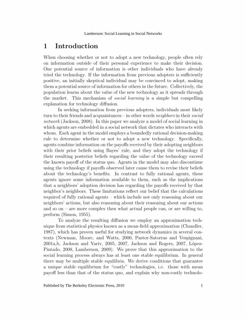
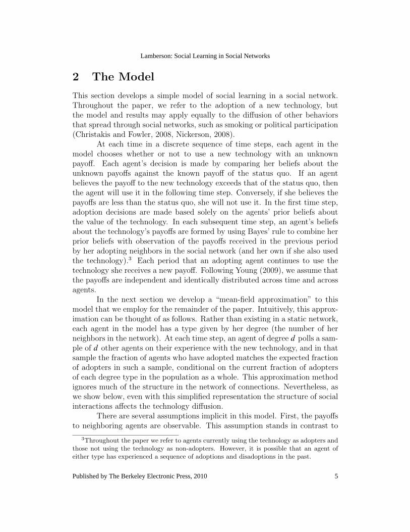
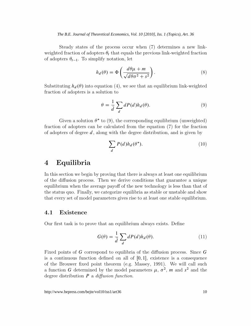
Figure 1: Three examples of a diffusion function G.�/ for a regular degree fournetwork.

Several aspects of the function G should be noted. First,

G.0/ D1

Nd

Xd

dP.d/hd .0/ D1

Nd

Xd

dP.d/ˆ�ms

�D ˆ

�ms

�> 0: (12)

That is, G.0/ is simply the fraction of agents with positive priors. Thus, zerois never an equilibrium of the process. This highlights a difference betweensocial learning and the contagion models of diffusion studied by Jackson andYariv (2005), Jackson and Rogers (2007), and Lopez-Pintado (2008), in whichzero is always an equilibrium. Here, as soon as the technology is availablesome agents will adopt based solely on their prior beliefs. Similarly,

G.1/ D1

Nd

Xd

dP.d/hd .1/ <1

Nd

Xd

dP.d/ D 1; (13)

so full adoption is also never an equilibrium. This stands in contrast to modelsof social learning in which the agents make use of an infinite number of obser-vations, where typically all of the agents settle on the same action (e.g. Balaand Goyal, 1998). These observations have welfare implications. Because thepayoff distribution is identical across agents and across time, the social opti-mum is always either no adoption or full adoption depending on the sign of theexpected payoff �. Equations (12) and (13) demonstrate that the agents neversettle precisely on the optimal level of adoption. Depending on the parametervalues there may be equilibria that are practically indistinguishable from noor full adoption, but in many cases there are not.

For some parameter values multiple equilibria exist. For example, asillustrated in Figure 1A, in a regular degree four network with mean payoff

11



� D 2, payoff variance �2 D 1, mean prior m D �3, and variance of priorss2 D 1, there are three equilibria: near zero, :26, or :99 (since this is a regularnetwork, � equals the actual fraction of adopters). Because the distributionof agents’ prior beliefs is strongly biased against adoption we would expectthe system to settle on the low adoption equilibrium, even though more than97 percent of draws from the payoff distribution are positive. Unfortunately,from a social welfare perspective, without forcing many of the agents to adoptinitially against their beliefs, the society will never gather enough evidenceregarding the positive payoffs of the technology to overcome their skepticismand reach the high adoption equilibrium.

In other cases, only a single equilibrium exists. In the previous example,agents’ were initially biased against adoption; only about one in a thousandagents began with a positive prior. If agents have more favorable priors weobserve a different pattern. Figure 1B depicts the graph of G.�/ for the sameparameter values as Figure 1A except that m has been increased from �3 to�1. In this case, a greater number of agents adopt initially, and observingthese early adopters’ payoffs convinces much of the rest of the population toadopt. Figure 1C illustrates a third possibility for the diffusion function. Theparameters that generate this curve are the same as those for Figure 1A exceptthat now the mean payoff � has been decreased from 2 to 1. In this case thesystem inevitably settles on near zero adoption.

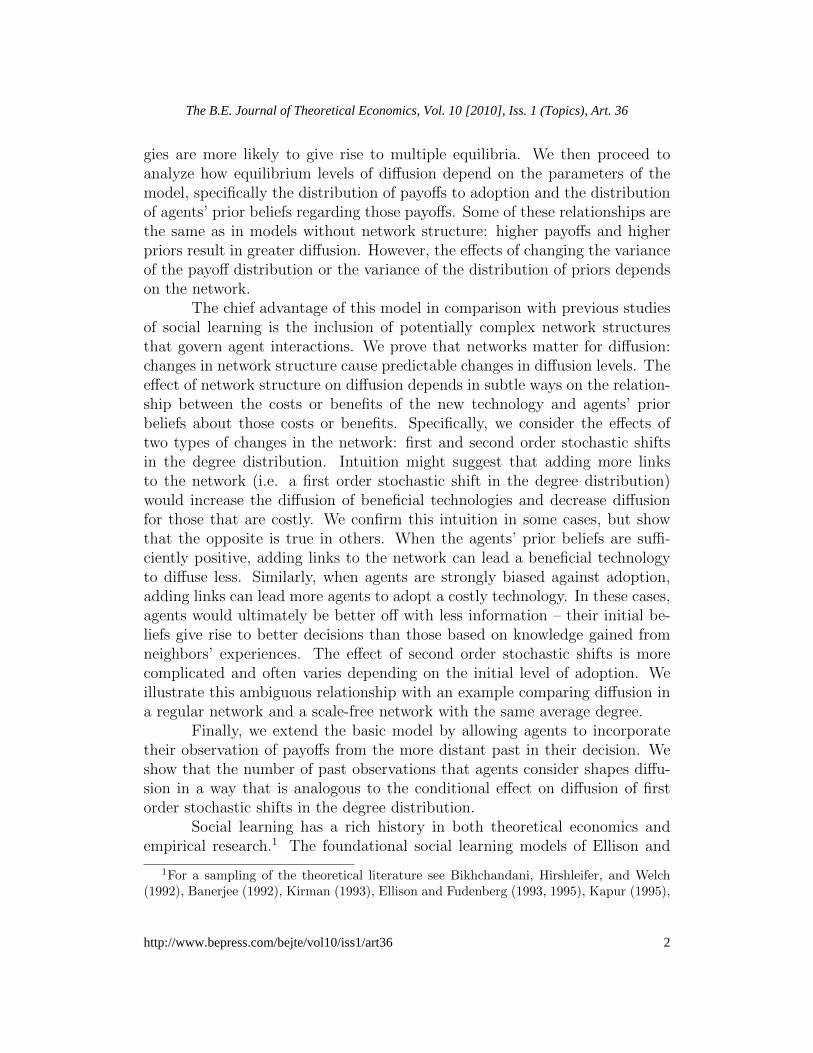
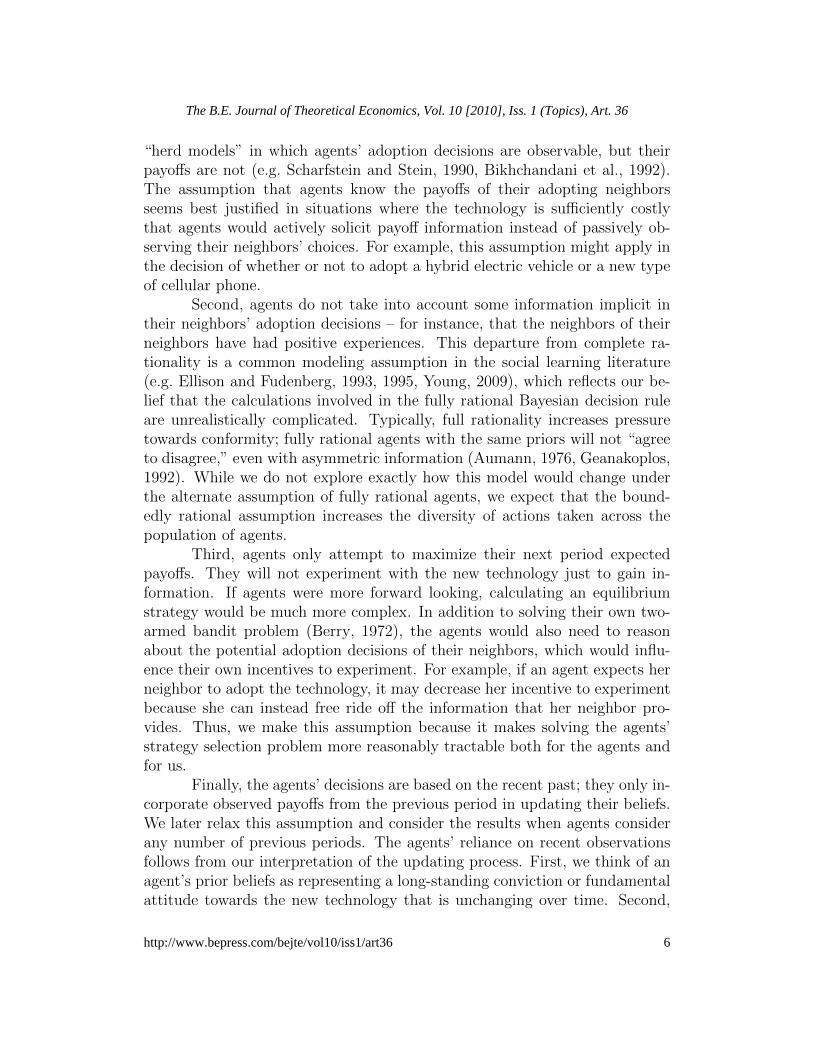
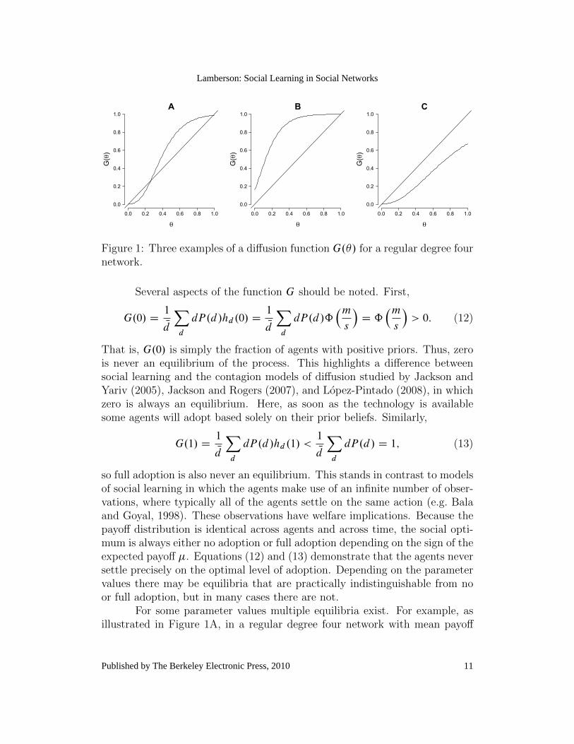
With other network degree distributions there may be many more equi-libria. Figure 2 plots an example with five equilibria. In this example � D 2,�2 D :25, m D �3 and s2 D :25. In the network one percent of the nodes havedegree fifty, while the rest of the nodes have an equal chance of having degreeone, two, three, four, or five.

4.2 Uniqueness for Costly Technologies

When � < 0 the technology offers less utility than the status quo on average.We call such a technology costly. When a technology is costly, as long asthe agents’ priors are not overly biased against adoption, there is a uniqueequilibrium to the social learning process.

Theorem 1. If � < 0 and

2�

�2<m

s2; (14)

then a diffusion function G with parameters �, �2, m, and s2 has a uniqueequilibrium regardless of the network structure.

12



0.0 0.2 0.4 0.6 0.8 1.0

0.0

0.2

0.4

0.6

0.8

1.0

θ

G(θ)

Figure 2: An example of a diffusion function G.�/ with five equilibria.

Theorem 1. If � < 0 and

2�

�2<m

s2; (14)

then a diffusion function G with parameters �, �2, m, and s2 has a uniqueequilibrium regardless of the network structure.

Proof. The reason for the unique equilibrium is that when � < 0 and (14)is satisfied, G is a decreasing function of � and therefore has a unique fixedpoint. The derivative of G with respect to � is

G 0.�/ D1

Nd

Xd

dP.d/@hd

@�.�/: (15)

13



The derivative of hd with respect to � is

@hd

@�.�/ D dˆ0

�d��Cmpd��2 C s2

�d��2 C 2�s2 � �2m

2.d��2 C s2/3=2: (16)

Thus the sign of @hd@�.�/ and therefore of G 0.�/ is the same as the sign of

d��2 C 2�s2 � �2m. When � < 0,

d��2 C 2�s2 � �2m < 2�s2 � �2m; (17)

which is negative whenever the condition (14) is satisfied.

This theorem illustrates the asymmetry between costly and benefi-cial technologies. For costly technologies, an external shock that adds moreadopters tends to be countered by a decrease in adoption as those new adopterslearn and communicate that the technology is costly. This “negative feedbackloop” tends to bring the system to equilibrium. For beneficial technologies,the system can come to rest at an equilibrium in which more agents wouldadopt if they knew about the benefits of adopting, but too few agents arecurrently adopting in order for the group to learn about those benefits. Anexternal shock that adds more adopters increases the number of agents whoknow about the benefits, who in turn can communicate that knowledge to theirneighbors leading to still further adoption. This results in a “positive feedbackloop,” which can move the system towards a higher adoption equilibrium.6

4.3 Stable and Unstable Equilibria

The mean-field analysis in the previous section identifies equilibria of the sociallearning process. In practice, randomness makes it unlikely for some of theseequilibria to be maintained. For example, because agents’ experiences arerandom draws from the payoff distribution, at any particular time or particularregion of the network these draws will fluctuate around the true mean of the

6For discussions of positive and negative feedbacks and multiple equilibria see Arthur(1996) and Sterman (2000).

14



0 20 40 60 80

0.0

0.2

0.4

0.6

0.8

1.0

A

Time Step

Frac

tion

Adop

ters

0.0 0.2 0.4 0.6 0.8 1.0

0.0

0.2

0.4

0.6

0.8

1.0

B

θ

G(θ)

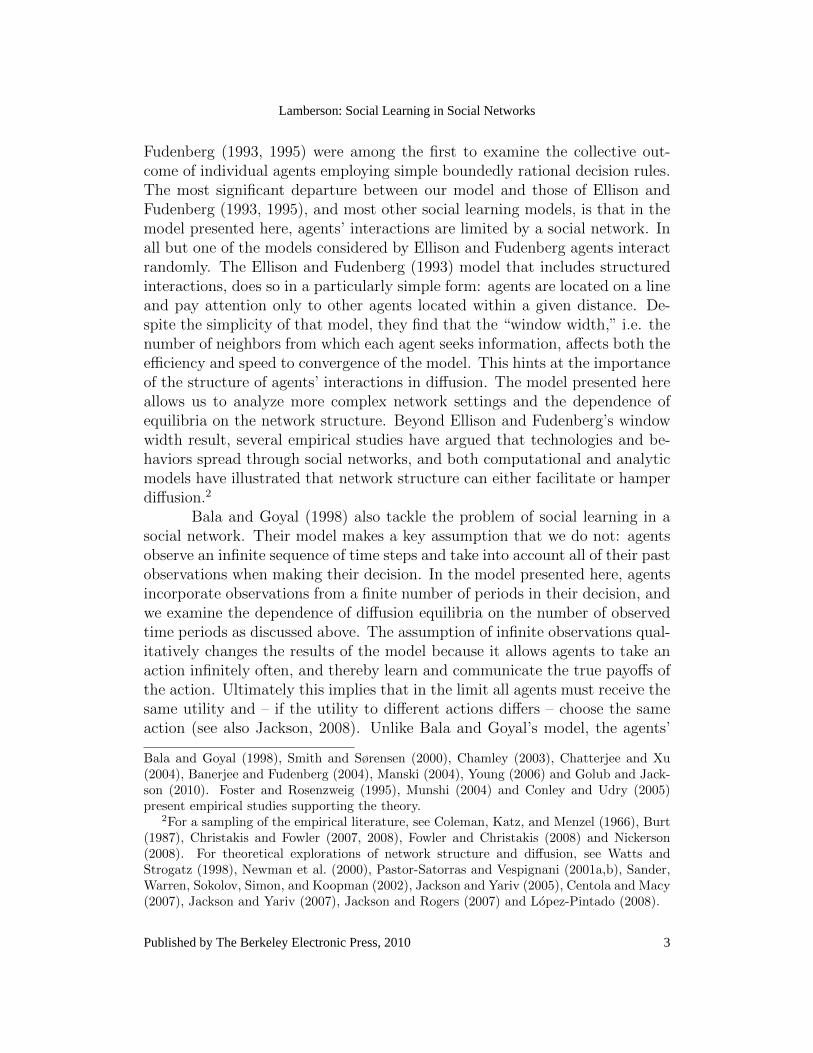
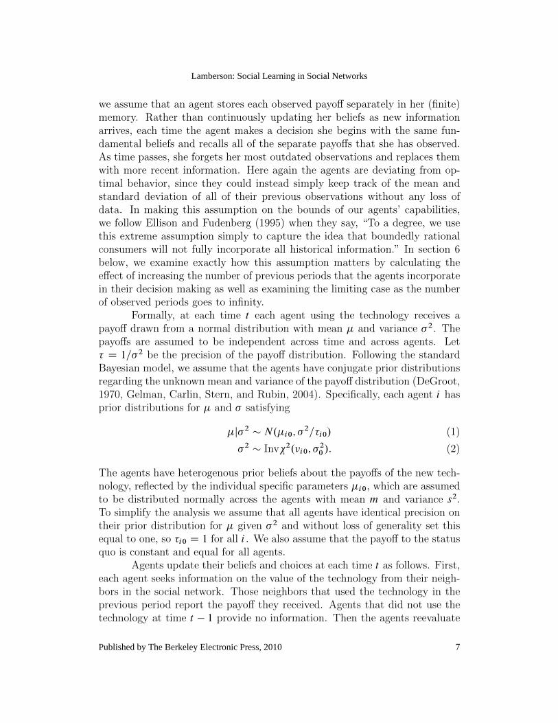
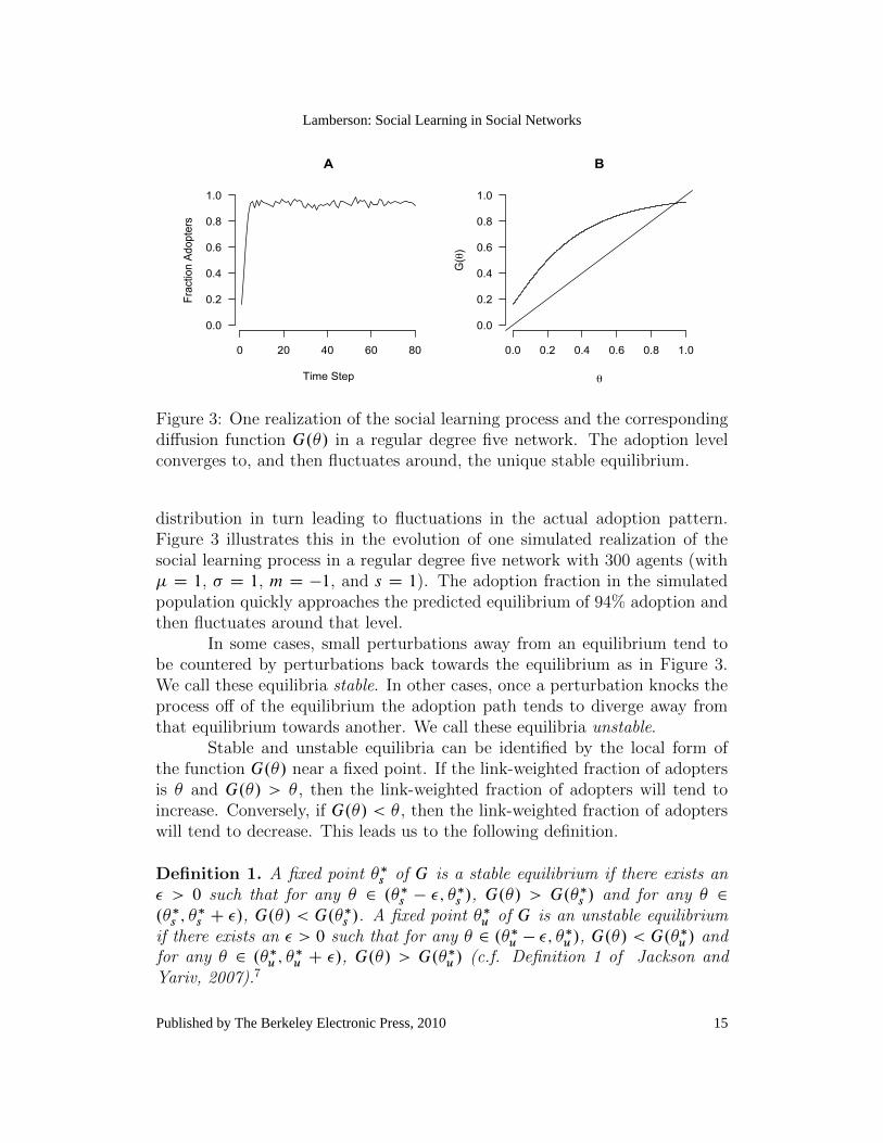
Figure 3: One realization of the social learning process and the correspondingdiffusion function G.�/ in a regular degree five network. The adoption levelconverges to, and then fluctuates around, the unique stable equilibrium.

distribution in turn leading to fluctuations in the actual adoption pattern.Figure 3 illustrates this in the evolution of one simulated realization of thesocial learning process in a regular degree five network with 300 agents (with� D 1, � D 1, m D �1, and s D 1). The adoption fraction in the simulatedpopulation quickly approaches the predicted equilibrium of 94% adoption andthen fluctuates around that level.

In some cases, small perturbations away from an equilibrium tend tobe countered by perturbations back towards the equilibrium as in Figure 3.We call these equilibria stable. In other cases, once a perturbation knocks theprocess off of the equilibrium the adoption path tends to diverge away fromthat equilibrium towards another. We call these equilibria unstable.

Stable and unstable equilibria can be identified by the local form ofthe function G.�/ near a fixed point. If the link-weighted fraction of adoptersis � and G.�/ > � , then the link-weighted fraction of adopters will tend toincrease. Conversely, if G.�/ < � , then the link-weighted fraction of adopterswill tend to decrease. This leads us to the following definition.

Definition 1. A fixed point ��s of G is a stable equilibrium if there exists an� > 0 such that for any � 2 .��s � �; �

�s /, G.�/ > G.��s / and for any � 2

.��s ; ��s C �/, G.�/ < G.�

�s /. A fixed point ��u of G is an unstable equilibrium

if there exists an � > 0 such that for any � 2 .��u � �; ��u /, G.�/ < G.�

�u / and

for any � 2 .��u ; ��u C �/, G.�/ > G.��u / (c.f. Definition 1 of Jackson and

Yariv, 2007).7

15



For example, the fixed points in both Figure 1B and Figure 1C arestable. The smallest and largest fixed points in Figure 1A are stable, while themiddle fixed point in Figure 1A is unstable. For the most part we are moreinterested in stable equilibria than unstable equilibria because it is highlyunlikely that the stochastic process will settle on an unstable equilibrium.Instead a realization of the model will tend to hover near a stable equilibriumas in Figure 3.

The following theorem collects several observations on stable and unsta-ble equilibria, which can be proven using simple Intermediate Value Theoremarguments along with the facts that G is continuous, G.0/ > 0 and G.1/ < 1.

Theorem 2. Consider a diffusion function G as in equation (11). Then theset of equilibria for G satisfy the following:

1. There is at least one stable equilibrium.2. The smallest equilibrium is stable.3. The largest equilibrium is stable.4. The ordered set of equilibria alternates between stable and unstable equi-

libria.

We are interested in how stable equilibria depend on the parametersof our model and the network structure; however, when there are multipleequilibria it is unclear what it means for certain parameters to generate moreor less diffusion. To better describe this dependence we define a function�G W Œ0; 1� ! .0; 1/, which we call the equilibrium function of the diffusionfunction G. For any � 2 Œ0; 1� with G.�/ < � let �G.�/ be the largest stableequilibrium of G that is less than � . For any � 2 Œ0; 1� with G.�/ � � let�G.�/ be the smallest stable equilibrium of G that is greater than or equal to� . The idea of the equilibrium function is that if we begin the social learningprocess specified by G with a link-weighted fraction of adopters � then we

7A fixed point �� of G may also be a degenerate fixed point, which under definition 1is neither stable nor unstable, if G0.��/ D 1: However, generically all fixed points of G areeither stable or unstable. By this we mean that any G with a degenerate fixed point �� canbe transformed by an arbitrarily small perturbation in the space of the model parametersinto another diffusion function QG without a degenerate fixed point and for any G without adegenerate fixed point any diffusion function generated by a sufficiently small perturbationof the model parameters will also have no degenerate fixed points. For the remainder of thepaper we assume that G has no degenerate fixed points.

16



0.0 0.2 0.4 0.6 0.8 1.0

0.0

0.2

0.4

0.6

0.8

1.0

θ

G(θ)

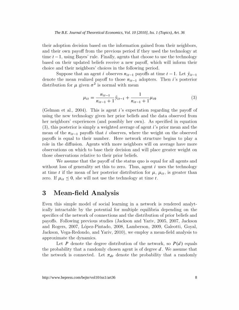
Figure 4: An example of a diffusion function G.�/ (solid) and the associatedequilibrium function �G.�/ (dashed).

expect the process to converge to near the stable equilibrium �G.�/.8 Figure

4 depicts an example.

Definition 2. A diffusion function G generates greater diffusion than a dif-fusion function QG if �G.x/ � � QG.x/ for all x 2 Œ0; 1� (c.f. Definition 3 ofJackson and Yariv, 2007).

Intuitively, a diffusion function G generates more diffusion than an-other QG if, regardless of the initial fraction of adopters, we expect the processspecified by G to converge to an equilibrium with a greater fraction of adoptersthan that specified by QG.

17



5 Comparative Statics

In this section we examine how changes in the model parameters and the socialnetwork affect equilibrium levels of diffusion.

5.1 Dependence on Model Parameters

First, we examine how the stable equilibria of a diffusion function G dependon the non-network parameters of the model, �, �2, m, and s2. We begin withthe following lemma, which shows that changes that increase the diffusionfunction lead to greater diffusion.

Lemma 1. If G.�/ � QG.�/ for all � then G generates greater diffusion thanQG (c.f. Proposition 1 of Jackson and Yariv, 2007).

Proof. For t 2 Œ0; 1�, define 't W Œ0; 1�! Œ0; 1� by

't.x/ D G.x/C t . QG.x/ �G.x//: (18)

So '0.x/ D G.x/ and '1.x/ D QG.x/ (i.e. 't is a homotopy from G to QG). Wecan determine how � QG relates to �G by examining how solutions to 't.x/ D xchange as t moves from zero to one. We extend the definition of stable andunstable equilibria to stable and unstable fixed points of 't.x/ in the obviousway and for each t define a function �t.x/ corresponding to 't.x/ in the sameway that �G.x/ is defined from G. Small increases in t can result in threechanges in the ordered set of fixed points of 't :

8When � is an unstable equilibrium the choice to set �G.�/ to be the next largest stableequilibrium as opposed to the next smaller stable equilibrium is arbitrary.

18



0.0 0.2 0.4 0.6 0.8 1.0

0.0

0.2

0.4

0.6

0.8

1.0

A

θ

G(θ

), G~(θ)

0.0 0.2 0.4 0.6 0.8 1.0

0.0

0.2

0.4

0.6

0.8

1.0

B

θ

φ G, φ G~

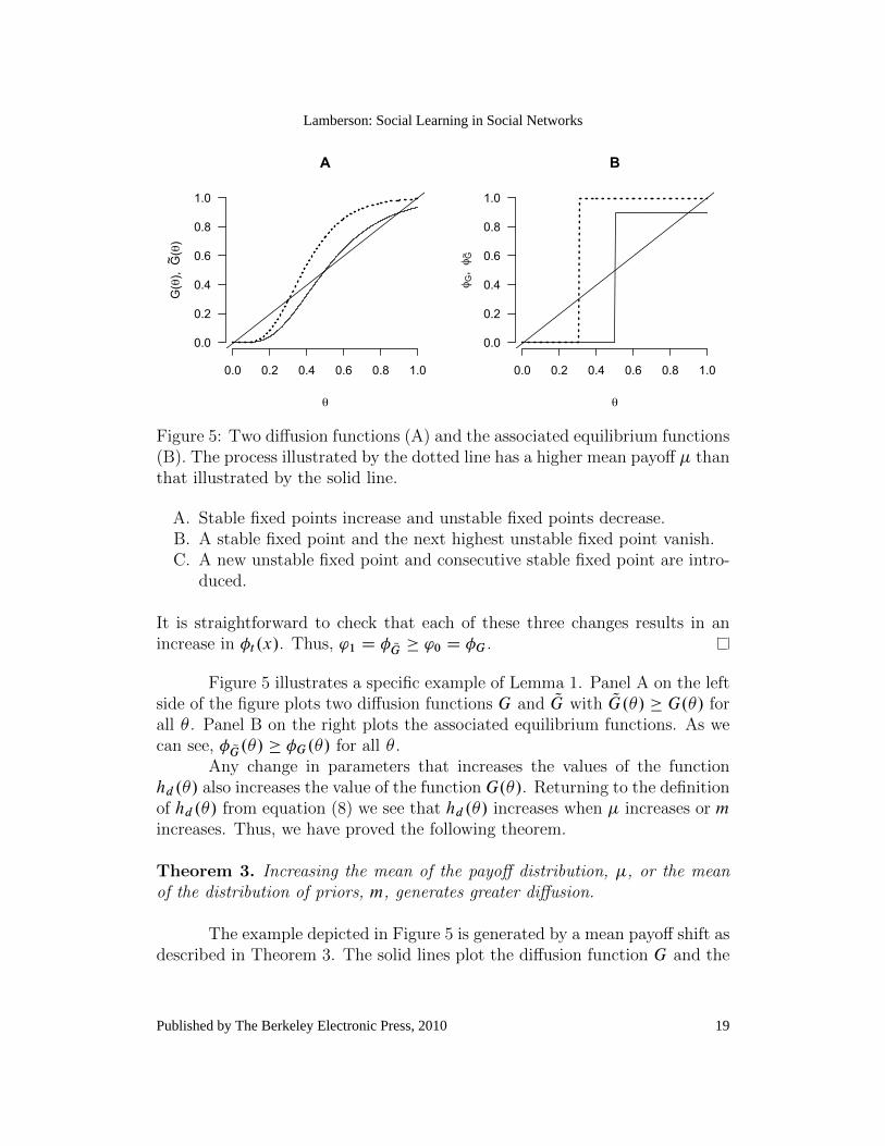
Figure 5: Two diffusion functions (A) and the associated equilibrium functions(B). The process illustrated by the dotted line has a higher mean payoff � thanthat illustrated by the solid line.

A. Stable fixed points increase and unstable fixed points decrease.B. A stable fixed point and the next highest unstable fixed point vanish.C. A new unstable fixed point and consecutive stable fixed point are intro-

duced.

It is straightforward to check that each of these three changes results in anincrease in �t.x/. Thus, '1 D � QG � '0 D �G .

Figure 5 illustrates a specific example of Lemma 1. Panel A on the leftside of the figure plots two diffusion functions G and QG with QG.�/ � G.�/ forall � . Panel B on the right plots the associated equilibrium functions. As wecan see, � QG.�/ � �G.�/ for all � .

Any change in parameters that increases the values of the functionhd .�/ also increases the value of the function G.�/. Returning to the definitionof hd .�/ from equation (8) we see that hd .�/ increases when � increases or mincreases. Thus, we have proved the following theorem.

Theorem 3. Increasing the mean of the payoff distribution, �, or the meanof the distribution of priors, m, generates greater diffusion.

The example depicted in Figure 5 is generated by a mean payoff shift asdescribed in Theorem 3. The solid lines plot the diffusion function G and the

19



associated equilibrium function �G with � D 1, �2 D 1, m D �5 and s D 1

for a regular degree ten network. The dotted lines show the diffusion functionQG and the associated equilibrium function � QG which has the same parameters

and network as for G but with � increased to 1.3.The effects of changes in �2 and s2 are conditional on the sign of d��C

m. Since d� > 0, if � and m are either both positive or both negative, thenthe sign of d�� C m is also positive or negative, respectively. Thus, if both� and m are positive then hd .�/ increases when �2 decreases or s2 decreases.This proves the following theorem.

Theorem 4. If both � and m are positive, decreasing the variance of the payoffdistribution �2 or the variance of the distribution of priors s2 generates greaterdiffusion. If both � and m are negative, increasing the variance of the payoffdistribution �2 or the variance of the distribution of priors s2 generates greaterdiffusion.

The results in Theorem 3 and 4 do not depend on the network struc-ture. The same relationships would hold if there was no structure to agentinteractions. However, when � and m have opposite signs, the effect of in-creasing or decreasing the variance in the payoff or prior distributions dependson the degree distribution of the network. Depending on the network, chang-ing the variance of the payoff or prior distribution can generate greater or lessdiffusion or have an ambiguous effect.

5.2 Dependence on Network Structure

This section examines the effect of changes in the network structure, as spec-ified by the degree distribution P , on the extent of the technology diffusion.We examine the effects of two types of changes in the network: first and secondorder stochastic dominance shifts in the degree distribution (Rothschild andStiglitz, 1970). A distribution P strictly first order stochastically dominates adistribution QP if for every nondecreasing function u W R! R;

DmaxXdD0

u.d/ QP .d/ <

DmaxXdD0

u.d/P.d/; (19)

where Dmax is the maximum degree of any node in the network. A distributionP strictly second order stochastically dominates a distribution QP if (19) holdsfor every nondecreasing concave function u W R! R:

20



First order stochastic dominance implies second order stochastic domi-nance, but not vice versa. If P and QP have the same mean, then the statementP second order stochastically dominates QP is equivalent to the statement QPis a mean preserving spread of P . Intuitively, one network first order stochas-tically dominates another if agents have more neighbors in the former thanthe latter. A network second order stochastically dominates another if there isless heterogeneity in the number of neighbors that agents have in the formerthan the latter.9

In our case, the role of the function u in equation (19) is played byhd .�/ and the role of the distribution P is played by dP= Nd D dP=EP Œd �.In order to understand the consequences of stochastic shifts in the degreedistribution, we need to understand when h is increasing and decreasing aswell as its concavity when viewed as a function of d . Since throughout thissection we will be interested in hd .�/ as a function of d , we will abuse notationby suppressing the dependence on � and simply write h.d/ for hd .�/, h

0.d/

for @hd .�/

@dand so on. Examining the first derivative of h, we see that

h0.d/ D �ˆ0�

d��Cmpd��2 C s2

�d��2 C 2�s2 � �2m

2.d��2 C s2/3=2: (20)

Thus the sign of h0.d/ depends on the sign of

d��2 C 2�s2 � �2m: (21)

If d��2C 2�s2� �2m > 0 then h0.d/ is positive. Suppose that � > 0. Then

d��2 C 2�s2 � �2m � 2�s2 � �2m; (22)

since d��2 � 0. The right hand side of (22) is greater than zero when

2�

�2>m

s2: (23)

So, when � > 0 and (23) holds, h is an increasing function of d for any � > 0.A similar argument shows that when � < 0 and

2�

�2<m

s2(24)

h is a decreasing function of d . In this case, Theorem 1 guarantees that thereis a unique equilibrium level of diffusion in both P and QP . Combining thiswith the definition of first order stochastic dominance and Lemma 1 proves:

9For an introduction to stochastic dominance and its role in network diffusion see Jackson(2008) or Lamberson (2009).

21



Theorem 5. Suppose that dP=EP Œd � strictly first order stochastically domi-nates d QP=E QP Œd �. If � > 0 (i.e. on average adopting the technology is benefi-cial) and

2�

�2>m

s2; (25)

then P generates greater diffusion than QP . If � < 0 (i.e. on average adoptingthe technology is costly) and

2�

�2<m

s2; (26)

then the unique equilibrium level of diffusion in the network with degree distri-bution QP is greater than the unique equilibrium level of diffusion in the networkwith degree distribution P .

We can think of a network that first order stochastically dominatesanother as providing the agents with more information, since on average theagents have more links to other agents. We would expect that for beneficialtechnologies, more information would aid diffusion. Theorem 5 confirms thisintuition, but only if the agents are not overly optimistic about the technologyto begin with, as captured by condition (25). If the agents’ prior beliefs aboutthe payoffs of the technology are sufficiently positive, so that (25) is violated,adding more links to the network can hinder diffusion. This stands in contrastto contagion models in which adding links always aids diffusion (Jackson, 2008,Lopez-Pintado, 2008).

On reflection, we might expect that when agents’ priors tend to bemore positive than the payoffs, adding links could decrease diffusion. Thatlogic leads to a condition that says if the fraction of payoffs that are positiveis greater than the fraction of agents with positive priors, i.e.

�

�2>m

s2; (27)

then first order stochastic shifts lead to greater diffusion. But the actualcondition (25) is more subtle. The intuitive condition (27) differs from theactual condition (25) by a factor of two on the left hand side. If we fix thedistribution of priors, and consider (25) as a condition on the payoffs, thenthe actual condition (25) is weaker than the intuitive condition (27). In otherwords, relative to the distribution of priors, the payoff distribution contributesmore to the marginal effect of degree on diffusion than we might expect.

This discrepancy arises because there is a non-trivial interaction be-tween the effect of adding links to the network and of changing the payoffdistribution due to the fact that only adopting agents can communicate payoff

22



information. Increasing the payoffs increases the number of adopting agents,which makes the effect of adding links stronger because those additional linksare more likely to connect to agents that have payoff information to share.Conversely, decreasing the payoff distribution weakens the effect of addinglinks, because those additional links are more likely to connect to non-adoptingagents who do not contribute any additional information.

Turning to second order stochastic dominance shifts, we have a similartheorem:

Theorem 6. Suppose that dP=EP Œd � strictly second order stochastically dom-inates d QP=E QP Œd �. If

h00.d/ > 0; (28)

then P generates greater diffusion than QP . If

h00.d/ < 0; (29)

then QP generates greater diffusion than P .

In Theorem 5 we were able to express conditions (25) and (26) in termsof the social learning parameters in an interpretable fashion. In the case ofsecond order stochastic changes in the degree distribution, as examined inTheorem 6, the analogous conditions become too complex to decipher whenwritten out in terms of the model parameters.10 Moreover, in many cases sec-ond order stochastic shifts in the degree distribution do not have a consistenteffect on diffusion because h is convex for some values of � and concave forothers.

This highlights another difference between network diffusion via sociallearning and via an epidemic model as considered by Jackson and Rogers(2007) or Lopez-Pintado (2008). In the model by Jackson and Rogers (2007),for example, a second order stochastically dominant degree distribution alwayshas a lower highest stable equilibrium. This holds because in the epidemicmodel the effect of adding edges is convex, essentially because adding a link toan agent increases both the chances that she becomes infected and the chancesthat she spreads the infection. In the social learning model the contributionof adding edges depends on the level of adoption, the distribution of payoffs,and the distribution of prior beliefs as well as the degree distribution.

10The second derivative of h with respect to d is

�2

4

"ˆ00

d��Cmpd��2C s2

!.d��2C 2�s2 � �2m/2

.d��2C s2/3Cˆ0

d��Cmpd��2C s2

!��2.d��2C 4�s2 � 3�2m/

.d��2C s2/5=2

#: (30)

23



0.0 0.2 0.4 0.6 0.8 1.0

0.0

0.2

0.4

0.6

0.8

1.0

θ

G(θ)

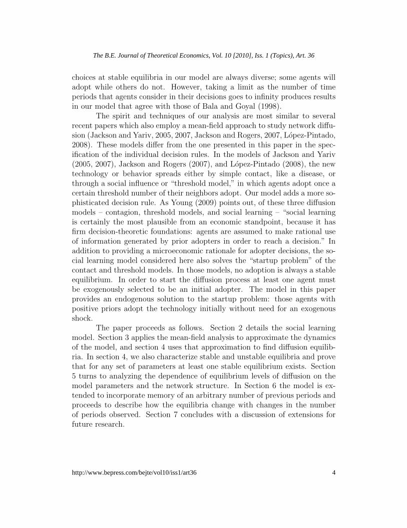
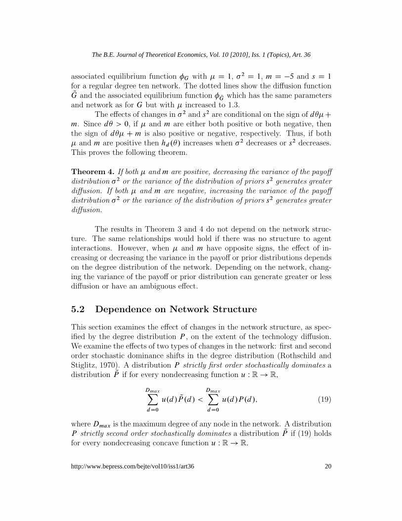
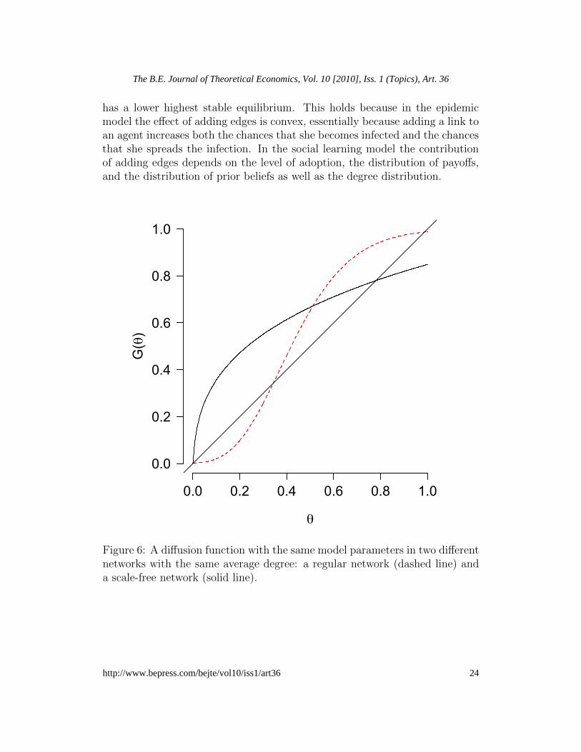
Figure 6: A diffusion function with the same model parameters in two differentnetworks with the same average degree: a regular network (dashed line) anda scale-free network (solid line).

has a lower highest stable equilibrium. This holds because in the epidemicmodel the effect of adding edges is convex, essentially because adding a link toan agent increases both the chances that she becomes infected and the chancesthat she spreads the infection. In the social learning model the contributionof adding edges depends on the level of adoption, the distribution of payoffs,and the distribution of prior beliefs as well as the degree distribution.

24



Figure 6 illustrates the phenomenon. The figure plots the diffusionfunction G with the same model parameters (� D 3, �2 D 1, m D �3 ands2 D 1) for a regular network (dashed line) and a scale-free network (i.e. onewith a power law degree distribution, solid line).11 The regular network secondorder stochastically dominates the scale-free network, but both have the sameaverage degree. Despite having the same average degree, these two degreedistributions generate vastly different dynamics. The scale free network has asingle equilibrium link-weighted fraction of adopters of 87.9%, which by equa-tion (10) corresponds to an actual adoption fraction of only 49.6%. Regardlessof the initial fraction of adopters, in the scale-free network we would expectthe process to converge to near 49.6% adoption. The regular network gives riseto two stable equilibria, one nearly indistinguishable from no adoption and an-other at approximately 98.6% adoption, as well as one unstable equilibrium at34.3%. For this network, unless the fraction of adoption is exogenously pushedbeyond the unstable equilibrium at 34.3% adoption, the process settles on theequilibrium near zero. However, if the population begins at a point above theunstable equilibrium, it then moves to the equilibrium at 98.6%, which is 49%higher than the equilibrium in the scale-free network. Thus, depending on theinitial adoption level, the regular network, which second order stochasticallydominates the scale-free network, can generate more or less diffusion.

6 Memory

Up to this point, agents’ adoption and disadoption decisions in the model arebased solely on payoffs from the previous period. In this respect, our modelfollows those considered by Ellison and Fudenberg (1993, 1995). In contrast,the model by Bala and Goyal (1998) allows agents to base their decisions onobservation of an infinite number of periods. At each stage in Bala and Goyal’smodel the agents update their priors based on new observations, and their newposterior becomes the prior for the following round. As discussed in section2, our agents behave differently. Instead, we think of each agent as storingher prior and each piece of the information she has accrued separately. Eachtime she makes an adoption decision, she recalculates her expected payoffbased on her prior and the information on payoffs that she has observed,but she will have forgotten observations which occurred sufficiently long ago.As described in the introduction, the finite and infinite observation cases are

11For this computation the maximum degree is fixed at 500. The power law exponent is2.3, the same as the exponent in the network of movie actors measured by Barabasi andAlbert (1999).

25



qualitatively different. In the infinite observation case, the population tendstowards conformity, while the finite observation case considered here alwaysmaintains some diversity.

While we take the one period approach of Ellison and Fudenberg in ouranalysis above, we now extend the model to incorporate an arbitrary finitenumber of observations. Suppose that agents base their adoption decision onobservations of payoffs from the previous k periods.12 Then, in equation (5)

we would replace d�t�1 withPkjD1 d�t�j . Carrying through the mean-field

analysis this leads to a new definition of the function hd .�/ in equation (8),

hd .�/ D ˆ

�dk��Cmpdk��2 C s2

�: (31)

None of the comparative statics analyzed in Theorems 3 and 4 are affected bythis change. Furthermore, differentiating h with respect to d as in equation(20), we obtain

h0.d/ D �kˆ0�

d�k�Cmpd�k�2 C s2

�d�k��2 C 2�s2 � �2m

2.d�k�2 C s2/3=2: (32)

Following the analysis in section 5.2, adding the parameter k also has noeffect on the conditions (25) and (26) or on the relationship between networkstructure and diffusion described in Theorem 5 or 6.

While the inclusion of larger numbers of observations does not changeany of the other comparative statics, it does itself have an effect on the equilib-rium. As is evident from equation (31), the role of the number of observationsterm k is similar to the role of degree. As with changes in degree, increasesin the number of observations cause increases in h when � > 0 and (25) issatisfied. Increases in k cause h to decrease when � < 0 and (26) is satisfied.

Combining these observations and applying Lemma 1 proves the fol-lowing theorem.

Theorem 7. Consider two diffusion functions G and QG with all of the sameparameters with the exception that the number of observations parameter k forG is greater than the number of observations parameter Qk for QG. If � > 0, soon average adopting the technology is beneficial, and

2�

�2>m

s2; (33)

12We implicitly assume that each agent observes at least k periods worth of payoffs beforeupdating her decision.

26



then G generates greater diffusion than QG. If � < 0, so on average adoptingthe technology is costly, and

2�

�2<m

s2; (34)

then QG generates greater diffusion than G.

So, the condition and direction of the effect of increases in the numberof observations on diffusion are the same as for first order stochastic shifts inthe degree distribution.

We can also ask, what happens in the limit as k approaches infinity?If � > 0 then as k approaches infinity G approaches one. Conversely, if� < 0 then G approaches zero. Thus, in the infinite observations limit thepopulation converges to the social optimum: all agents adopt if the technologyhas a positive average payoff and no agents adopt if the technology has anegative average payoff. In the infinite observation model of Bala and Goyal(1998), the population always converges to a consensus, but that consensusmay not be the optimal one. The reason for the discrepancy between ourresults and theirs lies in the distribution of prior beliefs. Their model allowsfor the possibility, for example, that all agents are sufficiently biased againstadoption of a technology that none of them ever try it. However, if at least oneagent has a sufficiently positive prior when � > 0, or a sufficiently negativeprior when � < 0, then the population in the Bala and Goyal model alsoconverges to the “correct” equilibrium. Because the model here assumes anormal distribution of prior beliefs and the mean-field approximation assumesan infinite population, this condition is always satisfied. Thus, taking thelimit as k approaches infinity, the model here reproduces the results of Balaand Goyal (1998) under the assumption that the distribution of agents’ priorshas sufficiently wide support.

7 Conclusion

In this paper we analyze a model of social learning in a social network. Thepaper contributes to two streams of literature – the literature on social learningas a mechanism for diffusion and the literature on diffusion in social networks– which were until now largely separate.13 Incorporating social network struc-ture in a standard social learning model adds realism; we would expect thatindividuals seek information from their friends and family. We prove that

13The papers by Bala and Goyal (1998, 2001) and Gale and Kariv (2003) are notableexceptions.

27



adding this network structure affects the diffusion. To the diffusion literature,the model presented here adds a microeconomic rationale for agents’ deci-sions, as opposed to a simple contagion or threshold model. Not surprisingly,we find that the collective dynamics of rational actors are more complex thanthe physics of disease spread. For example, in a contagion model, first orderstochastic shifts in the degree distribution always increase diffusion (Jacksonand Rogers, 2007). In contrast, in the model presented here, the effect of a firstorder stochastic shift depends on the payoffs to adoption and the agents’ priorbeliefs regarding those payoffs. We derive precise conditions for the relation-ships between first and second order stochastic shifts in the degree distributionand equilibrium levels of diffusion. In some cases we find these conditional ef-fects surprising. For example, adding links to a network can decrease diffusioneven when the social optimum is for all agents to adopt.

To analyze this model we employ a mean-field approximation, which re-quires assumptions that may not always be appropriate. For example, the ap-proximation results are likely to be less accurate in small networks or networksin which the degrees of neighboring agents are highly correlated. However,in many cases simulation results confirm that mean-field techniques providea good approximation to discrete dynamics (e.g. Newman and Watts, 1999,Newman et al., 2000, Newman, 2002).

The model and analysis employed in this paper open the door to the ex-ploration of other questions. First, in the model presented here, while agents’prior beliefs differ their preferences do not. Extending this model to includeheterogenous preferences is a logical next step. We may also consider thepossibility that those preferences are correlated with agents’ positions in thenetwork to reflect the fact that agents are more likely to have social ties withagents that are similar to them (i.e. the network exhibits homophily (McPher-son, Smith-Lovin, and Cook, 2001)). Second, one could add a dynamic to the“supply side” of the model to investigate how the results may be affected ifthe payoffs to the new technology changed over time or if multiple technologiescompeted for market share. The model raises the possibility of using informa-tion on network structure to tailor firm strategies to specific network contexts.Finally, the model offers a potential explanation for why technologies and be-haviors may diffuse to a greater extent in one community than another. Thiscould provide the basis for an empirical test of the model’s predictions andhelp us to better understand the mechanisms of diffusion and the role of socialstructure in the process.

28



References

Arthur, W. B. (1996): “Increasing returns and the new world of business,”Harvard Business Review, 74, 100–111.

Aumann, R. (1976): “Agreeing to disagree,” The Annals of Statistics, 4, 1236–1239.

Bala, V. and S. Goyal (1998): “Learning from neighbours,” Review of Eco-nomic Studies, 65, 595–621.

Bala, V. and S. Goyal (2001): “Conformism and diversity under social learn-ing,” Economic Theory, 17, 101–120.

Banerjee, A. (1992): “A simple model of herd behavior,” Quarterly Journal ofEconomics, 107, 797–817.

Banerjee, A. and D. Fudenberg (2004): “Word-of-mouth learning,” Gamesand Economic Behavior, 46, 1–22.

Barabasi, A. and R. Albert (1999): “Emergence of scaling in random net-works,” Science, 286, 509–512.

Berry, D. A. (1972): “A Bernoulli two-armed bandit,” The Annals of Mathe-matical Statistics, 43, 871–897.

Bikhchandani, S., D. Hirshleifer, and I. Welch (1992): “A theory of fads, fash-ion, custom, and cultural change as informational cascades,” The Journalof Political Economy, 100, 992–1026.

Burt, R. (1987): “Social contagion and innovation: Cohesion versus structuralequivalence,” American Journal of Sociology, 92, 1287.

Centola, D. and M. Macy (2007): “Complex contagions and the weakness oflong ties,” American Journal of Sociology, 113, 702–734.

Chamley, C. (2003): Rational Herds: Economic Models of Social Learning,Cambridge: Cambridge Univ Press.

Chandler, D. (1987): Introduction to Modern Statistical Mechanics, New York:Oxford.

Chatterjee, K. and S. Xu (2004): “Technology diffusion by learning from neigh-bours,” Advances in Applied Probability, 355–376.

Christakis, N. and J. Fowler (2007): “The spread of obesity in a large socialnetwork over 32 years,” New England Journal of Medicine, 357, 370–379.

Christakis, N. A. and J. H. Fowler (2008): “The colletive dynamics of smokingin a large social network,” The New England Journal of Medicine, 358, 2248–2258.

Coleman, J., E. Katz, and H. Menzel (1966): Medical Innovation: A DiffusionStudy, Indianapolis: Bobbs-Merrill Co.

Conley, T. and C. Udry (2005): “Learning about a new technology: Pineapplein Ghana,” Proceedings of the Federal Reserve Bank of San Francisco.

29



DeGroot, M. H. (1970): Optimal Statistical Decisions, New York: McGraw-Hill.

Ellison, G. and D. Fudenberg (1993): “Rules of thumb for social learning,”Journal of Political Economy, 101, 612–643.

Ellison, G. and D. Fudenberg (1995): “Word-of-mouth communication andsocial learning,” The Quarterly Journal of Economics, 110, 93–125.

Foster, A. and M. Rosenzweig (1995): “Learning by doing and learning fromothers: Human capital and technical change in agriculture,” Journal ofPolitical Economy, 103, 1176–1209.

Fowler, J. and N. Christakis (2008): “Dynamic spread of happiness in a largesocial network: Longitudinal analysis over 20 years in the Framingham HeartStudy,” British Medical Journal, 337, a2338.

Gale, D. and S. Kariv (2003): “Bayesian learning in social networks,” Gamesand Economic Behavior, 45, 329–346.

Galeotti, A., S. Goyal, M. O. Jackson, F. Vega-Redondo, and L. Yariv (2010):“Network games,” Review of Economic Studies, 77, 218–244.

Geanakoplos, J. (1992): “Common knowledge,” The Journal of EconomicPerspectives, 6, 53–82.

Gelman, A., J. B. Carlin, H. S. Stern, and D. B. Rubin (2004): Bayesian DataAnalysis, Boca Raton, FL: Chapman and Hall/CRC, second edition.

Jackson, M. O. (2008): Social and Economic Networks, Princeton, NJ: Prince-ton University Press.

Jackson, M. O. and B. W. Rogers (2007): “Relating network structure todiffusion properties through stochastic dominance,” The B.E. Journal ofTheoretical Economics (Advances), 7, 1–13.

Jackson, M. O. and L. Yariv (2005): “Diffusion on social networks,” Economiepublique, 16, 69–82.

Jackson, M. O. and L. Yariv (2007): “Diffusion of behavior and equilibriumproperties in network games,” American Economic Review, 97, 92–98.

Kapur, S. (1995): “Technological diffusion with social learning,” The Journalof Industrial Economics, 43, 173–195.

Kirman, A. (1993): “Ants, rationality, and recruitment,” The Quarterly Jour-nal of Economics, 108, 137–156.

Lamberson, P. J. (2009): “Linking network structure and diffusion throughstochastic dominance,” Technical Report FS-09-03, AAAI.

Lopez-Pintado, D. (2008): “Diffusion in complex social networks,” Games andEconomic Behavior, 62, 573–590.

Golub, B. and M. O. Jackson (2009): “Naive learning in social networks:Convergence, influence and the wisdom of crowds,” American EconomicJournal Microeconomics, 2, 112–149.

30



Manski, C. (2004): “Social learning from private experiences: The dynamicsof the selection problem,” Review of Economic Studies, 71, 443–458.

Massey, W. S. (1991): A Basic Course in Algebraic Topology, Graduate Textsin Mathematics, volume 127, New York: Springer.

McPherson, M., L. Smith-Lovin, and J. Cook (2001): “Birds of a feather:Homophily in social networks,” Annual Review of Sociology, 27, 415–444.

Munshi, K. (2004): “Social learning in a heterogeneous population: Tech-nology diffusion in the Indian green revolution,” Journal of DevelopmentEconomics, 73, 185–213.

Newman, M. E. J. (2002): “Spread of epidemic disease on networks,” PhysicalReview E, 66, 016128.

Newman, M. E. J., C. Moore, and D. J. Watts (2000): “Mean-field solution ofthe small-world network model,” Physical Review Letters, 84, 3201–3204.

Newman, M. E. J. and D. J. Watts (1999): “Scaling and percolation in thesmall-world network model,” Physical Review Volume E, 60, 7332–7342.

Nickerson, D. (2008): “Is voting contagious? Evidence from two field experi-ments,” American Political Science Review, 102, 49–57.

Pastor-Satorras, R. and A. Vespignani (2001a): “Epidemic dynamics and en-demic states in complex networks,” Physical Review E, 63.

Pastor-Satorras, R. and A. Vespignani (2001b): “Epidemic spreading in scale-free networks,” Physical Review Letters, 86, 3200–3203.

Rothschild, M. and J. Stiglitz (1970): “Increasing risk: I. A definition,” Jour-nal of Economic Theory, 2, 225–243.

Sander, L., C. Warren, I. Sokolov, C. Simon, and J. Koopman (2002): “Perco-lation on heterogeneous networks as a model for epidemics,” MathematicalBiosciences, 180, 293–305.

Scharfstein, D. and J. Stein (1990): “Herd behavior and investment,” TheAmerican Economic Review, 80, 465–479.

Simon, H. A. (1955): “A behavioral model of rational choice,” The QuarterlyJournal of Economics, 69, 99–118.

Smith, L. and P. Sørensen (2000): “Pathological outcomes of observationallearning,” Econometrica, 68, 371–398.

Sterman, J. (2000): Business Dynamics, New York: Irwin/McGraw-Hill.Watts, D. and S. Strogatz (1998): “Collective dynamics of ‘small-world’ net-

works,” Nature, 393, 440–442.Young, H. P. (2006): “The spread of innovations by social learning,” Working

Paper.Young, H. P. (2009): “Innovation diffusion in heterogeneous populations: Con-

tagion, social influence, and social learning,” American Economic Review,99.

31



Documents

The B.E. Journal of Theoretical Economicsmath.uchicago.edu/~shmuel/Network-course-readings...Fudenberg (1993, 1995) were among the rst to examine the collective out-come of individual