The B.E. Journal of Theoretical Economicshananye/Hanany_Klibanoff_BEJTE_2009.pdfels satisfying this property.3 We consider several applications of our general result in some detail,

The B.E. Journal of TheoreticalEconomics

AdvancesVolume 9, Issue 1 2009 Article 37

Updating Ambiguity Averse Preferences

Eran Hanany∗ Peter Klibanoff†

∗Tel Aviv University, [email protected]†Northwestern University, [email protected]

Recommended CitationEran Hanany and Peter Klibanoff (2009) “Updating Ambiguity Averse Preferences,” The B.E.Journal of Theoretical Economics: Vol. 9: Iss. 1 (Advances), Article 37.Available at: http://www.bepress.com/bejte/vol9/iss1/art37

Copyright c©2009 The Berkeley Electronic Press. All rights reserved.

Updating Ambiguity Averse Preferences∗

Eran Hanany and Peter Klibanoff

Abstract

Dynamic consistency leads to Bayesian updating under expected utility. We ask what it im-plies for the updating of more general preferences. In this paper, we characterize dynamicallyconsistent update rules for preference models satisfying ambiguity aversion. This characterizationextends to regret-based models as well. As applications of our general result, we characterizedynamically consistent updating for two important models of ambiguity averse preferences: theambiguity averse smooth ambiguity preferences (Klibanoff, Marinacci and Mukerji [Econometrica73 2005, pp. 1849-1892]) and the variational preferences (Maccheroni, Marinacci and Rustichini[Econometrica 74 2006, pp. 1447-1498]). The latter includes max-min expected utility (Gilboaand Schmeidler [Journal of Mathematical Economics 18 1989, pp. 141-153]) and the multiplierpreferences of Hansen and Sargent [American Economic Review 91(2) 2001, pp. 60-66] as spe-cial cases. For smooth ambiguity preferences, we also identify a simple rule that is shown tobe the unique dynamically consistent rule among a large class of rules that may be expressed asreweightings of the Bayes’ rule.

KEYWORDS: updating, dynamic consistency, ambiguity, regret, Ellsberg, Bayesian, consequen-tialism, smooth ambiguity

∗We thank Nabil Al-Najjar, Sandeep Baliga, Eddie Dekel, Jurgen Eichberger, Larry Epstein,Raphael Giraud, Simon Grant, Ian Jewitt, Massimo Marinacci, Sujoy Mukerji, Bob Nau, BenPolak, Chris Shannon, Marciano Siniscalchi, Tomasz Strzalecki, Kane Sweeney, Tim Van Zandtand especially Fabio Maccheroni for helpful comments and discussion. We also thank the co-editor, Federico Echenique, and two anonymous referees for their comments. Additional thanksto seminar audiences at INSEAD, HEC, Johns Hopkins, Northwestern and Technion and at FURXII, RUD ‘07, Fall ’07 Midwest Economic Theory, ESNASM ’08, the 3rd Israeli Game TheoryConference and the 3rd World Congress of the Game Theory Society. This research was partiallysupported by Grant No. 2006264 from the United States-Israel Binational Science Foundation(BSF), Jerusalem, Israel.

1 Introduction

A central question facing any theory of decision making under uncertainty ishow preferences are updated to incorporate new information. Since updatedpreferences govern future choices, it is important to know how they relateto information contingent choices made ex-ante. Dynamic consistency is therequirement that ex-ante contingent choices are respected by updated prefer-ences. This consistency is implicit in the standard way of thinking about adynamic choice problem as equivalent to a single ex-ante choice to which one iscommitted, and is thus ubiquitous in economic modeling. We formally de�nedynamic consistency in Section 2.2.Under subjective expected utility, updating preferences by applying Bayes�

rule to the subjective probability is the standard way to update. Why is thisso? Dynamic consistency is the primary justi�cation for Bayesian updating.Not only does Bayesian updating imply dynamic consistency, but, if updatingconsists of specifying a conditional probability measure for each (non-null)event, dynamic consistency implies these conditional measures must be theBayesian updates.1 The requirement that updating consists of specifying aconditional probability measure ensures closure for expected utility preferences�i.e., that each such preference remains an expected utility preference afterupdating.Since dynamic consistency and closure lead to a well-established theory of

updating for expected utility, it is important to ask what they imply for theupdating of more general preferences. Closure for a set of preferences meansthat each member of that set remains in the set after updating. In earlier work(Hanany and Klibano¤ [2007]), we began to address this issue by identifyingand characterizing the �rst dynamically consistent update rules satisfying clo-sure for the maxmin expected utility (MEU) model of decision-making underambiguity (Gilboa and Schmeidler [1989]).2 In this paper, we are able to sub-stantially generalize the approach taken there and characterize dynamicallyconsistent update rules for essentially all continuous, monotonic preferencesthat are ambiguity averse in that they satisfy the uncertainty aversion axiomintroduced in Schmeidler [1989] (i.e., have convex upper contour sets in utilityspace). Schmeidler�s axiom (stated in Section 2.2) is very commonly used todescribe ambiguity aversion in the literature and MEU is but one of many mod-

1See e.g., Proposition 6 in Hanany and Klibano¤ [2007] or Proposition 3.1 in Section 2.2.2Epstein and Schneider [2003] had previously investigated updating of MEU preferences

using a stronger notion of dynamic consistency (see our discussion of recursive dynamicconsistency in Section 6) and, as a result, to avoid a collapse to expected utility had torestrict attention to updating given a limited set of events (the so-called rectangular events).

1

Hanany and Klibanoff: Updating Ambiguity Averse Preferences

Published by The Berkeley Electronic Press, 2009

els satisfying this property.3 We consider several applications of our generalresult in some detail, characterizing dynamically consistent update rules sat-isfying closure for important speci�c models of ambiguity averse preferences:the smooth ambiguity preferences (Klibano¤, Marinacci and Mukerji [2005],henceforth KMM),4 the variational preferences (Maccheroni, Marinacci andRustichini [2006a], henceforth MMR) and regret-based models of ambiguityaversion, such as minimax regret with multiple priors (Hayashi [2008], Stoye[2008b]). We propose the �rst dynamically consistent update rules satisfyingclosure for these models.What is a main di¤erence in the implications of dynamic consistency when

updating ambiguity averse preferences rather than standard preferences? Con-sider Ellsberg�s three-color example, in which bets are made over the color ofa ball drawn randomly from an urn with 90 balls, of which 30 are black (B)and the remaining 60 are somehow divided between red (R) and yellow (Y ).Taking triples (uB; uR; uY ) 2 R3 to represent utility acts, i.e. state (color)contingent utility payo¤s, the typical preference (1; 0; 0) � (0; 1; 0) (bettingon black rather than red) and (0; 1; 1) � (1; 0; 1) (betting against black ratherthan against red) is inconsistent with expected utility but is consistent (andis one of the primary motivations for) many models of preferences under am-biguity. Let us introduce dynamics by supposing that after the ball is drawnfrom the urn, the decision maker (DM) is informed whether or not the ball isyellow.5 The DM is allowed to condition her choice of bets on this information.Notice that this conditioning opportunity does not expand the feasible set ofutility acts compared to the original problem of choosing between betting onB or on R �only the utility payo¤s (1; 0; 0) or (0; 1; 0) (and their convex com-binations, if randomization is considered) are achievable. The same applies tothe choice between betting on the event fB; Y g or on fR; Y g �even with con-ditioning allowed, only convex combinations of (1; 0; 1) or (0; 1; 1) are feasible.Ex-ante, then, the static and dynamic choice problems are the same. A DMwith the typical Ellsberg preferences is dynamically consistent in this problemif (1; 0; 0) is chosen over (0; 1; 0) when the dynamic problem is played out (i.e.,conditional on the event fB;Rg, betting on B is chosen over betting on R)

3For alternative notions of ambiguity aversion, see Epstein [1999] and Ghirardato andMarinacci [2002].

4See also Ergin and Gul [2009], Nau [2006], Neilson [2009], and Seo [2009] for relatedpreference analyses and Hansen [2007] for an application to macroeconomic risk. Whilesmooth ambiguity preferences may display a full range of ambiguity attitudes, we focusexclusively on the ambiguity averse subset of these preferences.

5Such dynamic extensions of Ellsberg have been considered before, e.g., Epstein andSchneider [2003], Hanany and Klibano¤ [2007].

2

The B.E. Journal of Theoretical Economics, Vol. 9 [2009], Iss. 1 (Advances), Art. 37

http://www.bepress.com/bejte/vol9/iss1/art37

and (0; 1; 1) is chosen over (1; 0; 1) when the dynamic problem is played out(i.e., conditional on the event fB;Rg, betting on fR; Y g is chosen over bettingon fB; Y g). Dynamic consistency creates a problem for the usual methods ofupdating preferences. To see this, observe that a choice of (1; 0; 0) over (0; 1; 0)conditional on fB;Rg from a feasible set consisting of this pair would directlycon�ict with a choice of (0; 1; 1) over (1; 0; 1) conditional on fB;Rg from afeasible set consisting of this latter pair. The con�ict results because, whenrestricted to the event fB;Rg, each pair involves exactly the choice of (1; 0)versus (0; 1). Therefore, to achieve dynamic consistency of the prototypicalambiguity averse preferences while ruling out updated preferences that giveweight to unrealized events, updating must depend on the ex-ante contingentplan and/or feasible set of acts.Why is dynamic consistency important enough to justify the additional

complications it necessitates under ambiguity aversion? The fundamental rea-son is that dynamically consistent updating results in higher (ex-ante) welfarethan any other form of updating. If a DM could choose an update rule, it wouldalways be optimal to choose a dynamically consistent one. This is a strongjusti�cation for investigating dynamically consistent updating �such updaterules are precisely what a DM should use. In sum, characterizing dynamicallyconsistent update rules is a way to characterize optimal update rules.There are two other approaches to modeling ambiguity averse preferences in

dynamic settings. One approach deals with recursive extensions (e.g., Epsteinand Schneider [2003], MMR [2006b], KMM [2009], Hayashi [2009]), while theother posits dynamic inconsistency and adopts (either explicitly or implicitly)assumptions, such as backward induction (e.g., Siniscalchi [2009]) or naiveignorance of the inconsistency, to pin down behavior. We compare them withour approach in some detail in Section 6, but want to mention here that inboth of these approaches updating is independent of the ex-ante contingentplan and feasible set of acts, thus these approaches cannot deliver dynamicconsistency for many events.The fact that dynamically consistent updating of preferences that are not

expected utility requires dependence on more than just the conditioning eventwas recognized by Machina [1989] and McClennen [1990]. Such updating isreferred to as non-consequentialist. Machina [1989] proposed a dynamicallyconsistent update rule in the context of preferences over objective lotteries,and this was later adapted by Machina and Schmeidler [1992] to satisfy dy-namic consistency and closure for probabilistically sophisticated preferencesover acts.6

6They show, in this latter context, that the rule is equivalent to updating beliefs by Bayes�

3



Capturing ambiguity averse behavior, however, requires models that go be-yond probabilistic sophistication. We would like to �nd, for a variety of suchmodels, dynamically consistent update rules that satisfy closure. In an earlycontribution in this direction, Eichberger and Grant [1997] succeed in char-acterizing a class of preferences quadratic in probabilities that allows for am-biguity aversion and is closed under Machina-Schmeidler updating. Why clo-sure? Economists often choose to work with speci�c models because they aretractable and parsimoniously capture desired behavioral features (frequentlyexpressed through axioms on preferences). A theory of updating will be mosthelpful when it allows the use of the same type of model throughout the prob-lem under consideration. At a normative level, if properties of a model havestrong appeal before updating, it would seem odd for this appeal to disappearafter updating. Thus, desired properties imposed on the ex-ante preferencesshould also be imposed on the updated preferences, as this has the advantageof delivering the most relevant and interesting theory.Unfortunately, the Machina-Schmeidler update rule fails closure for any

set of preferences that includes non-probabilistically sophisticated members,as long as the preferences satisfy essentially the Savage [1954] axioms with-out the Sure-Thing Principle (Savage�s P2) (see Epstein and Le Breton [1993]).Similarly, one can show that this rule is not closed for smooth ambiguity prefer-ences or for variational preferences (both of which violate Savage�s P4 as well asP2). In this paper, we successfully develop and characterize dynamically con-sistent update rules satisfying closure, for models ranging from imposing onlyambiguity aversion, continuity and monotonicity to those requiring particularfamilies of ambiguity averse preferences such as smooth ambiguity preferences,variational preferences, MEU preferences or multiplier preferences.Why are these models of particular interest? The smooth ambiguity model

simultaneously allows: separation of ambiguity attitude from perception ofambiguity; �exibility and non-constancy in ambiguity attitude; subjective and�exible perception of which events are ambiguous; the tractability of smoothpreferences; and expected utility as a special case for any given ambiguityattitude. Furthermore, its modeling of ambiguity attitude allows tools andinsights from the usual treatment of risk attitude under expected utility to beimported. The variational preferences model is an elegant and highly �exiblemodel most notable for including and relating widely used models such asthe MEU model and the robust-control/multiplier preferences of Hansen and

rule while simultaneously updating risk preferences in a speci�c, non-consequentialist way.See also Segal [1997] and Wakker [1997] who investigate alternative non-consequentialistupdate rules.

4



Sargent [2001] as special cases. The multiplier preferences of Hansen andSargent [2001] model ambiguity or model uncertainty using relative entropywith respect to a reference subjective probability measure and have proventractable in applications.In addition to specializing our characterization of dynamically consistent

updating for these models, we provide some more results of interest for each.Among rules satisfying closure for smooth ambiguity preferences, a rule weconstruct is shown to be the unique dynamically consistent rule that is areweighting of Bayes�rule. We also show that it has other good properties,for example, it is commutative, in the sense that only the total informationavailable and not the order in which it arrives is important for updating.Among rules satisfying closure for variational preferences, we show that a largeset of dynamically consistent update rules imply that multiplier preferencesshould be updated by applying Bayes�rule to the reference measure.What allows us to characterize dynamic consistency for such a broad class

of preferences? The key is characterizing global (conditional) optimality of theex-ante optimum. For convex feasible sets and preferences that have convexupper contour sets, this comes down to the existence of a measure in theintersection of two sets: the set of measures corresponding to hyperplanessupporting the conditional indi¤erence curve at the ex-ante optimum and theset of measures supporting the relevant feasible set at the ex-ante optimum.7

1.1 An illustration of our approach: the smooth rule

To give some understanding of our results and the type of argument thatunderlies them, we brie�y describe a dynamically consistent update rule pro-posed in this paper satisfying closure for ambiguity averse smooth ambiguitypreferences and apply it to the dynamic Ellsberg example. Consider pref-erences having the following representation: beliefs are represented by a �-nite support probability measure � over the set � of all probability measures� over a state space S, risk attitudes are represented by a von Neumann-Morgenstern expected utility function u : X ! R over a set of lotteries X,and ambiguity attitudes are represented by a strictly increasing, concave anddi¤erentiable function � : u (X) ! R, such that for all acts f and h, f % h() E�� (E�u � f) � E�� (E�u � h), where E is the expectation operator.Think of an update rule de�ned by updating � to a new belief, denoted �E;g,

7In Hanany and Klibano¤ [2007] on updating MEU, the former set was available �di-rectly� in the form of the updated set of measures in the representation of conditionalpreferences. The generalization from this speci�c form is one of the key theoretical insightsof the present paper and what enables the vastly expanded scope of application.

5



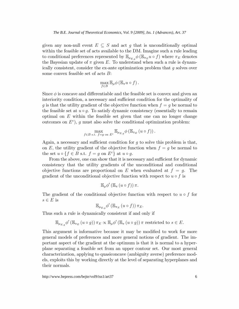
given any non-null event E � S and act g that is unconditionally optimalwithin the feasible set of acts available to the DM. Imagine such a rule leadingto conditional preferences represented by E�E;g� (E�Eu � f) where �E denotesthe Bayesian update of � given E. To understand when such a rule is dynam-ically consistent, consider the ex-ante optimization problem that g solves oversome convex feasible set of acts B:

maxf2B

E�� (E�u � f) .

Since � is concave and di¤erentiable and the feasible set is convex and given aninteriority condition, a necessary and su¢ cient condition for the optimality ofg is that the utility gradient of the objective function when f = g be normal tothe feasible set at u � g. To satisfy dynamic consistency (essentially to remainoptimal on E within the feasible set given that one can no longer changeoutcomes on Ec), g must also solve the conditional optimization problem:

maxf2B s.t. f=g on Ec

E�E;g� (E�E (u � f)) .

Again, a necessary and su¢ cient condition for g to solve this problem is that,on E, the utility gradient of the objective function when f = g be normal tothe set u � ff 2 B s.t. f = g on Ecg at u � g.From the above, one can show that it is necessary and su¢ cient for dynamic

consistency that the utility gradients of the unconditional and conditionalobjective functions are proportional on E when evaluated at f = g. Thegradient of the unconditional objective function with respect to u � f is

E��0 (E� (u � f))�.

The gradient of the conditional objective function with respect to u � f fors 2 E is

E�E;g�0 (E�E (u � f))�E.

Thus such a rule is dynamically consistent if and only if

E�E;g�0 (E�E (u � g))�E / E��0 (E� (u � g))� restricted to s 2 E.

This argument is informative because it may be modi�ed to work for moregeneral models of preferences and more general notions of gradient. The im-portant aspect of the gradient at the optimum is that it is normal to a hyper-plane separating a feasible set from an upper contour set. Our most generalcharacterization, applying to quasiconcave (ambiguity averse) preference mod-els, exploits this by working directly at the level of separating hyperplanes andtheir normals.

6



An example of a dynamically consistent rule we propose in the smoothambiguity setting is the smooth rule de�ned by setting

�E;g (�) =� (�)� (E) �0(E�(u�g))

�0(E�E (u�g))P�2�

� (�) � (E) �0(E�(u�g))�0(E�E (u�g))

if � (E) > 0,

(and equals 0 otherwise). Notice that when the smooth rule is used to de�ne�E;g,

E�E;g�0 (E�E (u � g))�E

/ E��0 (E�E (u � g))�0 (E�(u � g))�0 (E�E(u � g))

�(E)�E

= E��0 (E�(u � g))� for s 2 E

verifying dynamic consistency. We will see that this rule has many nice prop-erties.A numerical example of the smooth rule serves to show how it generates

dynamically consistent preferences in the dynamic Ellsberg example describedabove. Recall that the relevant state space is S = fB;R; Y g correspondingto the three colors that might be drawn from the urn. We assume that theDM has smooth ambiguity preferences with � a half-half distribution overthe distributions �� (1

3; 23�; 2

3(1 � �)) for � 2

�13; 23

. This is consistent

with the fact that the chance of drawing a black ball is known to be one-third and the ex-ante symmetry of the situation. Lotteries are monetary andevaluated by their expected value (i.e., u is the identity) and �(x) = �e��xwhere � > 0 so that the DM displays constant absolute ambiguity aversionwith coe¢ cient � (see KMM [2005]). We can verify, using Jensen�s inequality,that these preferences display the modal Ellsberg choices: (1; 0; 0) � (0; 1; 0)and (0; 1; 1) � (1; 0; 1). Now consider updating on the event that the ball isnot yellow so that E = fB;Rg. According to the smooth rule, conditionalpreferences are represented by

VE;g(u � f) = �[E�1=3E(u � f)]�E;g(�1=3) + �[E�2=3E

(u � f)]�E;g(�2=3)

where �E;g(��) =

�0(E�� (u�g))�0 E��E(u�g)

!�(�)��(E)

P�2f 13 ; 23g

�0�E��

(u�g)�

�00@E

��E

(u�g)

1A�(�)��(E)

and ��E = (1

1+2�; 2�1+2�

; 0) for � 2

�13; 23

.

7



For the feasible set B1 = co f(1; 0; 0); (0; 1; 0)g corresponding to the �rstEllsberg choice pair, u�g = (1; 0; 0).8 Applying the smooth rule, �E;(1;0;0)(��) =(3+6�)e

�( 11+2�

)

5e3�5 +7e

3�7. Similarly, for the feasible set B2 = co f(1; 0; 1); (0; 1; 1)g corre-

sponding to the second Ellsberg choice pair, u�g = (0; 1; 1) and �E;(0;1;1)(��) =(3+6�)e

�( 2�1+2�

)

5e2�5 +7e

4�7. Notice that when u � g = (1; 0; 0) the updated belief puts more

weight on the measure giving higher conditional probability of black than itdoes when u�g = (0; 1; 1). If, for example, � = 1, then �E;(1;0;0)(�

13 ) � 0:4588,

while �E;(0;1;1)(�13 ) � 0:3757. What is an intuition for why these weights are

di¤erent? When facing problem B1, preferring (1; 0; 0) reveals that the DMmust in some sense be assigning more prior weight to the scenario � = 1

3where

red has a low probability relative to black. Upon updating, this will meanthat such scenarios continue to get more weight than they would under sym-metric prior weighting. When facing problem B2, however, preferring (0; 1; 1)reveals that the DM must in the same sense be assigning less prior weight tothe scenario � = 1

3. After updating then, this scenario will continue to get

less weight than under symmetric prior weighting. Further calculation showsthat with smooth rule updating, as dynamic consistency requires, (1; 0; 0) isconditionally optimal within B1 and (0; 1; 1) is conditionally optimal withinB2.By way of contrast, consider standard Bayesian updating in this exam-

ple, given by �E(��) = 1+2�

4for � 2

�13; 23

, so that �E(�

13 ) = 5

12� 0:4167. In

comparing (1; 0; 0) and (0; 1; 0), observe that the distribution of conditional ex-pected utilities for (1; 0; 0), (3

5w.prob. 5

12; 37w.prob. 7

12), is a mean-preserving

spread of the distribution (25w.prob. 5

12; 47w.prob. 7

12) for (0; 1; 0). Since � is

strictly concave, this implies (0; 1; 0) �E (1; 0; 0), and thus Bayesian updatingviolates dynamic consistency for such a DM.What happens if we use the Machina-Schmeidler update rule in this ex-

ample? In our context, their rule is equivalent to saying that if ex-ante pref-erences are represented by the functional V (u � f) for all acts f , then up-dated preferences after learning E, given that g was unconditionally optimalwithin the feasible set of acts B, are represented by V (u � fEg) for all actsf where fEg denotes the act equal to f on E and g on Ec. In the example,V (u�f) � E�� (E�u � f) and thus the updated preferences are represented byV (u � fEg) � E�� (E�u � fEg). Substituting yields

�12e��(

13f(B)+ 2

9f(R)) � 1

2e��(

13f(B)+ 4

9f(R))

8We use co to denote the convex hull operator. We take the convex hull of the availableacts to re�ect the fact that the DM may randomize among them.

8



when g = (1; 0; 0) and

�12e��(

13f(B)+ 2

9f(R)+ 4

9) � 1

2e��(

13f(B)+ 4

9f(R)+ 2

9)

when g = (0; 1; 1). One can show these updated preferences are not smoothambiguity preferences over acts.9 Therefore the Machina-Schmeidler rule, al-though dynamically consistent, does not allow one to talk about updatingbeliefs �, nor does it produce updated preferences that satisfy the propertiesof the smooth ambiguity model (something that the ex-ante preferences dosatisfy), so it cannot even be described as updating a combination of tastes,�, and beliefs, �.The rest of the paper is organized as follows. Section 2 contains an ex-

position of the framework and notation, formally de�nes dynamic consistencyand presents our main result characterizing dynamic consistency in ambiguityaverse preference models. This result is applied in Section 3 to characterize dy-namically consistent update rules satisfying closure for the smooth ambiguitymodel. We then derive a novel update rule, the smooth rule mentioned above,which is shown to be the unique dynamically consistent rule among a largeclass of rules that may be expressed as reweightings of Bayes�rule. We de-scribe additional desirable properties of this update rule, including invarianceto the order in which information arrives (commutativity) and a strict ver-sion of dynamic consistency. We then show several impossibility results whenstrengthening dynamic consistency. Section 4 applies the general characteri-zation result to the representation developed in Cerreia-Vioglio, Maccheroni,Marinacci and Montrucchio [2008] (henceforth CMMM) and to rules satisfyingclosure for variational preferences. We also construct some consistent updaterules for variational preferences. The result on dynamically consistent updat-ing of multiplier preferences is here as well. Section 5 explains how our resultsextend to updating regret-based models, including minimax regret with mul-tiple priors. Related literature, including recursive approaches and dynamicinconsistency, is discussed in Section 6. The �nal section contains a brief con-clusion. All proofs not appearing in the main text are collected in AppendixA.

9Not even if restricted to acts of the form fEg.

9



2 Dynamic consistency and updating ambigu-ity averse preferences

2.1 Setting and notation

Consider an Anscombe-Aumann framework [1963], where X is the set of allsimple (i.e., �nite-support) lotteries over a set of consequences Z, S is a �niteset of states of nature and A is the set of all acts, i.e., functions f : S ! X.10

Abusing notation, x 2 X is also used to denote the constant act for which8s 2 S, f(s) = x.Let B denote the set of all non-empty subsets of acts B � A such that B

is convex (with respect to the usual Anscombe-Aumann mixtures) and com-pact (according to the norm taking the maximum over states and Euclideandistance on lotteries in X). Elements of B are considered feasible sets andtheir convexity could be justi�ed, for example, by randomization over acts.11

Compactness is needed to ensure the existence of optimal acts.Let P denote the set of preference relations (i.e., complete and transitive

binary relations) % on the acts A satisfying the following quite standard as-sumptions: preferences (i) are non-degenerate (i.e., f � h for some acts f; h),(ii) are mixture continuous (i.e., the sets f� 2 [0; 1] j �f + (1� �)i % hg andf� 2 [0; 1] j h % �f + (1� �)ig are closed), (iii) are weakly monotonic (i.e.,f (s) % h (s) for all s 2 S implies f % h) and (iv) when restricted to constantacts, obey the von Neumann-Morgenstern expected utility axioms.Given V : RS ! R such that (i) V is non-constant and continuous and (ii)

a � b implies V (a) � V (b) for all a; b 2 RS, and given a non-constant vonNeumann-Morgenstern utility function u : X ! R, the functional V (u � �) :A ! R represents a unique preference in P. Without loss of generality, �x aparticular normalization of u throughout the analysis. Consider a pair (V; u)where V and u satisfy these conditions. Let denote the set of all suchpairs. Each element of is thus associated with a unique preference %2 P.Conversely, given any preference in P there exists a unique u and at least oneV such that (V; u) 2 represents it.12 For any %2 P, it will be useful toidentify the set of interior acts, int (A) � ff 2 A j u � f is in the interior of10The lottery structure, per se, is not essential. Extension of all of our analysis to the

case where X is a general convex subset of a vector space is straightforward.11The important implication of convexity with respect to mixtures will be that, if u :

X ! R is a von Neumann-Morgenstern utility function, feasible sets have a convex imagein utility space, i.e., fu � f j f 2 Bg is convex. Alternatively, one could assume the latterdirectly.12Existence may be shown along the lines of Lemma 67 in the Appendix of CMMM [2008].

10



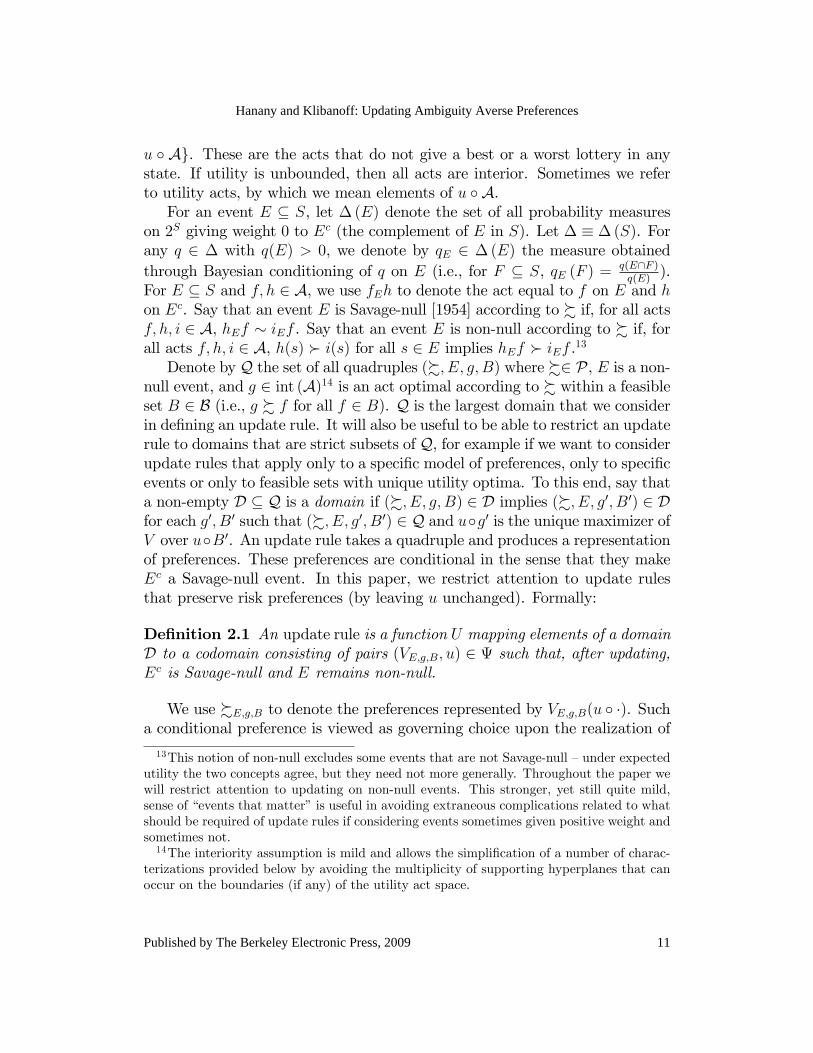
u � Ag. These are the acts that do not give a best or a worst lottery in anystate. If utility is unbounded, then all acts are interior. Sometimes we referto utility acts, by which we mean elements of u � A.For an event E � S, let �(E) denote the set of all probability measures

on 2S giving weight 0 to Ec (the complement of E in S). Let � � �(S). Forany q 2 � with q(E) > 0, we denote by qE 2 �(E) the measure obtainedthrough Bayesian conditioning of q on E (i.e., for F � S, qE (F ) =

q(E\F )q(E)

).For E � S and f; h 2 A, we use fEh to denote the act equal to f on E and hon Ec. Say that an event E is Savage-null [1954] according to % if, for all actsf; h; i 2 A, hEf � iEf . Say that an event E is non-null according to % if, forall acts f; h; i 2 A, h(s) � i(s) for all s 2 E implies hEf � iEf .13Denote by Q the set of all quadruples (%; E; g; B) where %2 P, E is a non-

null event, and g 2 int (A)14 is an act optimal according to % within a feasibleset B 2 B (i.e., g % f for all f 2 B). Q is the largest domain that we considerin de�ning an update rule. It will also be useful to be able to restrict an updaterule to domains that are strict subsets of Q, for example if we want to considerupdate rules that apply only to a speci�c model of preferences, only to speci�cevents or only to feasible sets with unique utility optima. To this end, say thata non-empty D � Q is a domain if (%; E; g; B) 2 D implies (%; E; g0; B0) 2 Dfor each g0; B0 such that (%; E; g0; B0) 2 Q and u�g0 is the unique maximizer ofV over u�B0. An update rule takes a quadruple and produces a representationof preferences. These preferences are conditional in the sense that they makeEc a Savage-null event. In this paper, we restrict attention to update rulesthat preserve risk preferences (by leaving u unchanged). Formally:

De�nition 2.1 An update rule is a function U mapping elements of a domainD to a codomain consisting of pairs (VE;g;B; u) 2 such that, after updating,Ec is Savage-null and E remains non-null.

We use %E;g;B to denote the preferences represented by VE;g;B(u � �). Sucha conditional preference is viewed as governing choice upon the realization of

13This notion of non-null excludes some events that are not Savage-null �under expectedutility the two concepts agree, but they need not more generally. Throughout the paper wewill restrict attention to updating on non-null events. This stronger, yet still quite mild,sense of �events that matter�is useful in avoiding extraneous complications related to whatshould be required of update rules if considering events sometimes given positive weight andsometimes not.14The interiority assumption is mild and allows the simpli�cation of a number of charac-

terizations provided below by avoiding the multiplicity of supporting hyperplanes that canoccur on the boundaries (if any) of the utility act space.

11



the conditioning event E.15 Recall from the Introduction that, generally, al-lowing dependence on g and/or B is necessary for dynamic consistency underambiguity aversion. In some speci�c applications, we may be able to maintainconsistency while imposing independence from either g or B (but not both).For example, when considering update rules for smooth ambiguity preferences(in Section 3) we limit attention to rules depending on B only through g.Another example, as we explicitly remark after Theorem 2.1 in the next sub-section, is that all of our results hold when one limits attention to feasible setswhere u � g is unique, an environment where g is unimportant given B.

2.2 Dynamically consistent update rules

Dynamic consistency of one form or another has often been put forward as arationality criterion and thus, from a normative point of view, it is importantto identify rules that satisfy some version of this property. Moreover, fromthe normative point of view, optimal acts are the most important for dynamicconsistency to be satis�ed on because those are the acts that are chosen. Un-der dynamic consistency, optimal contingent plans remain optimal accordingto updated preferences. Therefore dynamically consistent updating necessar-ily maximizes ex-ante welfare among all update rules. Another normativeargument in favor of dynamic consistency is the dominated choice argumentdescribed in the context of an example in Section 6.2. Dynamic consistencyalso makes it easier to describe an individual planning ahead and to makewelfare statements in dynamic models because it is only under dynamic con-sistency that ex-ante and ex-post preferences agree on optimal feasible choices.Our axiom requires that, for each feasible set of acts, B, the update rule guar-antees, for any preference and any non-null conditioning event E, if g is chosenwithin B, it remains optimal conditionally. Formally,

Axiom 2.1 DC (Dynamic Consistency). For any (%; E; g; B) 2 D, if f 2 Bwith f = g on Ec, then g %E;g;B f .

This formalization of dynamic consistency appeared in Hanany and Klibano¤[2007] and is related to ideas and concepts in earlier literature such as Machina[1989], McClennen [1990], Segal [1997] and Grant, Kajii and Polak [2000].16

Recall from the Introduction that dependence of conditional preference on g

15For a discussion of the observability of conditional preferences see Appendix A.2 ofHanany and Klibano¤ [2007].16For a more detailed discussion of the relation to other de�nitions, see Hanany and

Klibano¤ [2007] and the discussion of recursive approaches in Section 6.1 of this paper.

12



and B is needed, in general, to attain dynamic consistency under ambiguityaversion. With ambiguity aversion, the weighting of states supporting thechoice of g from B is typically di¤erent than that supporting the choice ofsome g0 optimal in B0. It is quite natural, then, that g and/or B also af-fect the manner in which new information changes the DM�s view of theseuncertainties through updating.Observe that conditional optimality of g is checked against all f 2 B such

that f and g agree on Ec. Why check conditional optimality only against theseacts? Dynamic consistency is relevant only ceteris paribus, i.e., when exactlythe same consequences occur on Ec. To make clear why this is reasonable,consider an environment where the DM has a �xed budget to allocate acrossbets on various events. It would be nonsensical to require that the ex-anteoptimal allocation of bets remained better than placing all of one�s bets onthe realized event. This justi�es the restriction of the conditional comparisonsto acts that agree on Ec.Is there a way to describe the set of dynamically consistent update rules for

ambiguity averse preferences? We give a characterization of dynamic consis-tency that applies to update rules that produce representations of preferencessatisfying Schmeidler�s [1989] uncertainty aversion axiom. Schmeidler�s axiomsays that f % h implies �f + (1� �)h % h for � 2 [0; 1], and is equivalent inour setting to the quasiconcavity of V (i.e., preferences are convex in utilityspace). All smooth ambiguity preferences that are ambiguity averse in thesense of KMM [2005] satisfy this condition, as do all variational preferences,and the general uncertainty averse preferences studied by CMMM [2008], sothis includes a very large and interesting class of models.17 Formally, then,we restrict attention to update rules satisfying the following property that wehave verbally described above:

(i) (uncertainty/ambiguity aversion) all VE;g;B in the codomain of the updaterule are quasiconcave.

Letting Y denote the family of all update rules satisfying the above prop-erty, Y will be the largest family for which we describe the rules that aredynamically consistent.

17What about preferences that are not quasiconcave (i.e., that violate Schmeidler�s [1989]axiom)? The methods we describe will still apply if one is willing to update these so thatthe conditional preferences satisfy Schmeidler�s axiom. However, if one wants to allow non-quasiconcavity after updating, while the existence of dynamically consistent rules is easyto show, the general characterization of such rules would su¤er from all of the substantialdi¢ culties in characterizing global maxima of non-quasiconcave problems, and is thereforebeyond the scope of this paper.

13



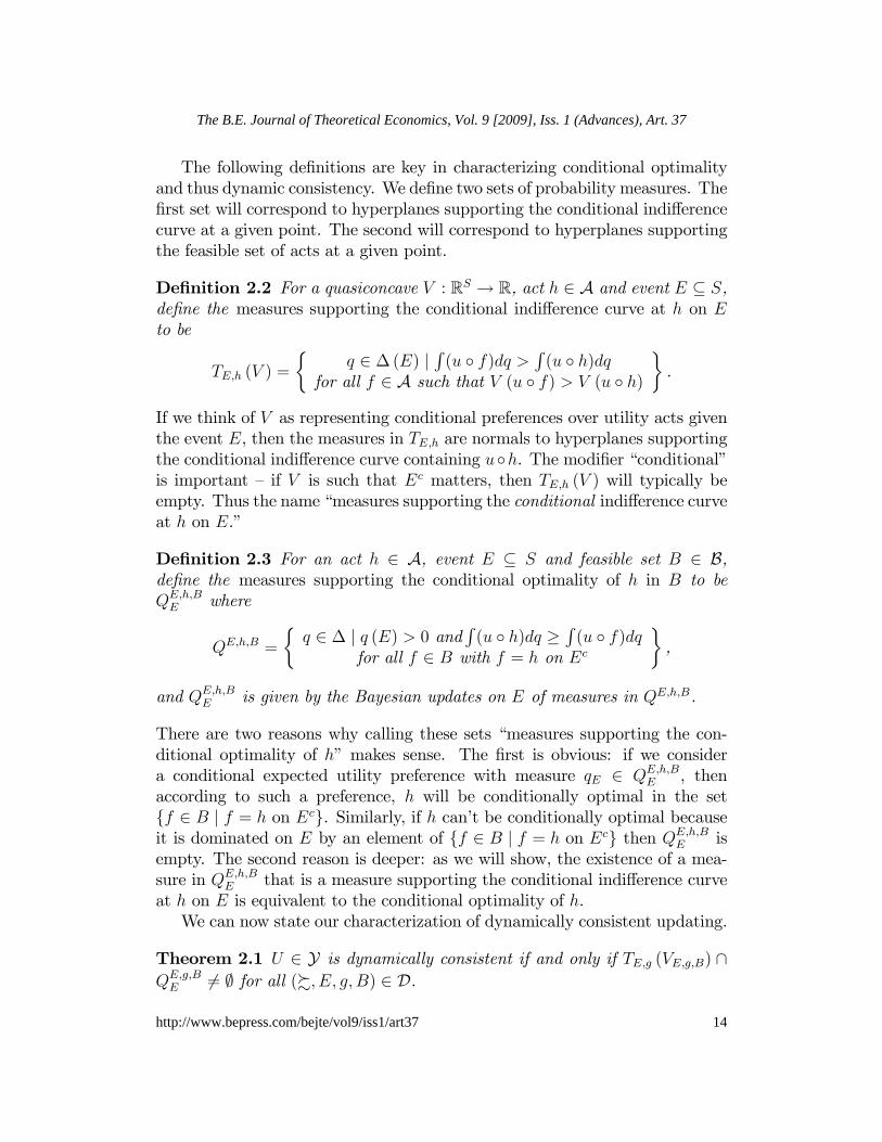
The following de�nitions are key in characterizing conditional optimalityand thus dynamic consistency. We de�ne two sets of probability measures. The�rst set will correspond to hyperplanes supporting the conditional indi¤erencecurve at a given point. The second will correspond to hyperplanes supportingthe feasible set of acts at a given point.

De�nition 2.2 For a quasiconcave V : RS ! R, act h 2 A and event E � S,de�ne the measures supporting the conditional indi¤erence curve at h on Eto be

TE;h (V ) =

�q 2 �(E) j

R(u � f)dq >

R(u � h)dq

for all f 2 A such that V (u � f) > V (u � h)

�.

If we think of V as representing conditional preferences over utility acts giventhe event E, then the measures in TE;h are normals to hyperplanes supportingthe conditional indi¤erence curve containing u�h. The modi�er �conditional�is important � if V is such that Ec matters, then TE;h (V ) will typically beempty. Thus the name �measures supporting the conditional indi¤erence curveat h on E.�

De�nition 2.3 For an act h 2 A, event E � S and feasible set B 2 B,de�ne the measures supporting the conditional optimality of h in B to beQE;h;BE where

QE;h;B =

�q 2 � j q (E) > 0 and

R(u � h)dq �

R(u � f)dq

for all f 2 B with f = h on Ec

�,

and QE;h;BE is given by the Bayesian updates on E of measures in QE;h;B.

There are two reasons why calling these sets �measures supporting the con-ditional optimality of h�makes sense. The �rst is obvious: if we considera conditional expected utility preference with measure qE 2 QE;h;BE , thenaccording to such a preference, h will be conditionally optimal in the setff 2 B j f = h on Ecg. Similarly, if h can�t be conditionally optimal becauseit is dominated on E by an element of ff 2 B j f = h on Ecg then QE;h;BE isempty. The second reason is deeper: as we will show, the existence of a mea-sure in QE;h;BE that is a measure supporting the conditional indi¤erence curveat h on E is equivalent to the conditional optimality of h.We can now state our characterization of dynamically consistent updating.

Theorem 2.1 U 2 Y is dynamically consistent if and only if TE;g (VE;g;B) \QE;g;BE 6= ; for all (%; E; g; B) 2 D.

14



This theorem provides a test for dynamic consistency of an update rule forambiguity averse preferences. First, given an event E, a feasible set B, and anact g unconditionally optimal within B, one can calculate QE;g;BE . If the imagein utility space of the set of feasible acts agreeing with g on Ec is smooth atu � g, QE;g;BE will be a singleton and can be found by di¤erentiation. Second,apply the candidate update rule to produce a representation of the updatedpreferences, VE;g;B. Third, calculate TE;g (VE;g;B). If, for example, VE;g;B issmooth at u�g this is no more complicated than usual di¤erentiation. Finally,see if the two sets intersect.The intuition is quite familiar from convex optimization: g will be con-

ditionally optimal within ff 2 B j f = g on Ecg if and only if there exists ahyperplane containing u� g that separates u�ff 2 B j f = g on Ecg from theutility acts conditionally better than u � g. Each hyperplane in utility spacemay be uniquely associated with a probability measure on the state space.The proof in Appendix A shows that the measures in TE;g (VE;g;B) \ QE;g;BE

exactly correspond to such separating hyperplanes.

Remark 2.1 Can we say anything special about update rules that do notdepend on g (given E and B)? Using the characterization in Theorem 2.1,we can show that such dynamically consistent update rules generally exist.However, they may be very restrictive in the ambiguity they permit afterupdating. For an illustration of this in the context of MEU, see Example 1 inHanany and Klibano¤ [2007]. As an alternative, less restrictive, approach toindependence from g, one could limit attention to feasible sets having a uniqueoptimum. The characterization in Theorem 2.1 remains true when restrictedto these sets. However, for later, more specialized results in the paper to gothrough, a slightly larger collection of feasible sets is needed. In this regard,note that one domain D to which Theorem 2.1 applies limits attention tofeasible sets for which u � g is uniquely optimal in u � B (i.e., there may bemultiple optima in B, but each generates the same utility act). If we take thisdomain and replace �f = g on Ec�with �f(s) s g(s) on Ec�in the de�nitionsof dynamic consistency and of QE;h;BE , we arrive at an application of Theorem2.1 where the choice of g is unimportant. Speci�cally, given B allowed bythis domain, further dependence of the update rule on g would never a¤ectdynamic consistency. With this domain restriction and the above-mentionedreplacement, all of the subsequent results in the paper and their proofs (withappropriate replacements of = with s if necessary) remain true.What about update rules that depend on B only through g? In this case, kinksin preferences can cause di¢ culties in achieving dynamic consistency (see e.g.,Proposition 7 in Hanany and Klibano¤ [2007]). In Section 3, we explore such

15



rules in detail for the (non-kinked) smooth ambiguity model.

Above, we suggested that calculation of TE;g (VE;g;B) amounted to di¤er-entiation if VE;g;B is smooth at u � g. In fact, the set TE;g (VE;g;B) is closelyrelated to a general di¤erential notion developed in Greenberg and Pierskalla[1973] for use in quasiconvex analysis. The de�nition below is adapted fromtheir paper and, up to normalization, simpli�es, for monotone and quasicon-cave functions, to the usual gradient at points of continuous di¤erentiabilitywhenever the gradient is non-zero.18

De�nition 2.4 Given a function I : RS ! R, its Greenberg-Pierskalla su-perdi¤erential at a is

@?I (a) =

�r : 2S ! R j r is bounded and additive and�

b 2 RS : I (b) > I (a)��b 2 RS :

Rbdr >

Radr � .

The next result says that we can replace TE;g (VE;g;B) in our characteriza-tion by the Greenberg-Pierskalla superdi¤erential of VE;g;B at u � g (or, sinceit is the only relevant part, only the conditional probability measures in thissuperdi¤erential):

Proposition 2.1 U 2 Y is dynamically consistent if and only if@?VE;g;B (u � g) \QE;g;BE 6= ; for all (%; E; g; B) 2 D.

This result is helpful in that it facilitates the use of gradients when avail-able. In the next section, we apply Proposition 2.1 to characterize dynamicallyconsistent update rules satisfying closure for ambiguity averse smooth ambigu-ity preferences. In the subsequent section, we apply our results to do the samefor the CMMM [2008] representation and variational preferences. Recall fromthe Introduction, when we say that an update rule satis�es closure for a set ofpreferences, we mean that both unconditional and conditional preferences arerestricted to that set. For example, if one wishes to restrict ex-ante preferencesto be variational preferences (i.e., to obey the axioms in MMR [2006a]) then itwill be most desirable to have an update rule that generates only variationalpreferences. Similarly, if one thinks it appropriate or useful to further restrictto multiplier preferences (i.e., to obey the axioms in Strzalecki [2008]), then anupdate rule de�ned on and generating only multiplier preferences will be of in-terest. No dynamically consistent update rules have been previously proposedsatisfying closure for either smooth ambiguity or variational preferences.18Since we consider updating only on non-null events, points with zero gradients do not

play a role in our analysis. We are grateful to Fabio Maccheroni for bringing the Greenberg-Pierskalla superdi¤erential to our attention and his substantial help and suggestions regard-ing the proposition on this and its proof.

16



3 Dynamically consistent updating of smoothambiguity preferences

In this section we investigate dynamically consistent update rules satisfyingclosure for ambiguity averse smooth ambiguity preferences. Let PSM denotethe set of smooth ambiguity preference relations over A (KMM [2005]).19 Forany preference%2 PSM , there exists a countably additive probability measure,�, over the set �, a von Neumann-Morgenstern expected utility function,u : X ! R and a strictly increasing function � : u (X)! R, such that 8f; h 2A, f % h () E�� (E�u � f) � E�� (E�u � h), where E is the expectationoperator. We will assume that � is di¤erentiable and concave. According toKMM, concavity of � re�ects ambiguity aversion. If � is degenerate, we adoptthe convention that � is the identity (with a degenerate �, � is irrelevant for%). For simplicity, we will also assume that the support of � is �nite. Letsupp(�) denote this support.Say that (V; u) 2 is an ambiguity averse smooth ambiguity represen-

tation whenever V (a) = E�� (E�a) for all a 2 RS. Such a V is completelydetermined by specifying � and �. Let SM denote the set of all such (V; u).Each element of SM is thus associated with a preference %2 PSM . To updateambiguity averse smooth ambiguity preferences we consider rules de�ned onan appropriate subset of quadruples (%; E; g; B) �speci�cally, DSM is the setof all elements of Q such that %2 PSM . Note that the only events in DSM arethose for which

P�2supp(�) � (�)� (E) > 0 as they are the non-null events in

the sense de�ned in Section 2.1.We consider update rules U � Y satisfying:

(i) (closure for ambiguity averse smooth ambiguity preferences) the domainis DSM and the codomain is SM ,

(ii) (preservation of ambiguity attitude) �E;g;B = �, and

(iii) (independence from feasible sets) VE;g;B1 = VE;g;B2 for all (%; E; g; B1); (%; E; g; B2) 2 DSM .

Property (i) re�ects the scope of this particular application of our results�we want to update within the class of ambiguity averse smooth ambiguity

19The framework in Klibano¤, Marinacci and Mukerji [2005] is not precisely an Anscombe-Aumann framework as the acts there need not have lottery consequences. However theirstate space S is assumed to be a product space with an ordinate that is [0; 1] and is treatedas a randomizing device. Thus, their theoretical development could be easily adapted to thesetting here. See Seo [2009] for an alternative axiomatization and model.

17



preferences. Since this class of preferences separates tastes (risk and ambi-guity attitudes) from beliefs, property (ii) extends the common notion thatnew information should a¤ect beliefs but not a¤ect tastes to encompass am-biguity attitudes in addition to the previously assumed preservation of riskattitudes. Property (iii) is assumed mainly because update rules satisfying itare in a natural sense simpler than those requiring dependence on B througha channel other than g, and because we can �we shall see that even withthis restriction interesting dynamically consistent update rules exist for thisclass of preferences. The fact that we are able to summarize dependence onthe feasible set through g stems from the smoothness of the preferences underconsideration.20

For these preferences, a given %, and even a given V , may be representedby multiple (�; �) pairs. In KMM, (�; �) are pinned down by consideringmore preference information than simply %. When we characterize dynam-ically consistent update rules in this section, we �x a function selecting aparticular (�; �) representation for each % that is to be updated. Note thatone can imagine the selection function being based on information outside thepresent framework, for example the preferences over second-order acts usedand discussed in KMM to pin down the characteristics of � and �. Given sucha selection function, a formula for updating (�; �) determines a well-de�nedupdate rule. Since update rules in U are required to satisfy properties (ii) and(iii) above, for the remainder of this section, an update rule in U will be iden-ti�ed with a mapping taking � to an updated measure �E;g, with the selectionrule implicitly �xed in the background.Given V (a) = E�� (E�a), an updated representation VE;g (a) could be writ-

ten as E��E;g� (E�a), where ��E;g satis�es ��E;g (� (E)) = 1. Notice that such aVE;g may also be written as E�E;g� (E�Ea) where

Pf�2supp(�E;g)j�E=�g �E;g (�) =

��E;g (�) for all � 2 �(E). We �nd it convenient to work with such represen-tations. Any �E;g determines a unique ��E;g in this way. Thus, to specify anupdate rule in U we can and will specify conditional measures �E;g rather than��E;g. Of course this relationship is not one-to-one �all �E;g corresponding tothe same ��E;g identify the same update rule in U (i.e., result in the same VE;g).An example of an update rule in U is Bayes�rule (i.e., Bayesian updating of

beliefs). Given (%; E; g; B) 2 DSM , applying Bayes�rule produces �E;g where

�E;g (�) =� (�)�(E)P

�2supp(�)� (�) �(E)

.

20In contrast, for models with kinks, (iii) would lead to the non-existence of dynamicallyconsistent updates. See Hanany and Klibano¤ [2007] for proof in the MEU case.

18



Dynamic consistency is intimately connected with Bayesian updating underexpected utility. In fact, the following result shows that dynamic consistencyjusti�es adopting Bayes�rule when preferences are expected utility.

Proposition 3.1 Any update rule in U with domain restricted so that % areexpected utility (i.e., � is a¢ ne) and that satis�es DC must produce the sameconditional preferences as Bayes�rule.

What does dynamic consistency say about updating smooth ambiguitypreferences beyond expected utility? We can use Proposition 2.1 to char-acterize the dynamically consistent rules in U . We will also show that thischaracterization is not vacuous � such rules exist. Unfortunately, it is nolonger true that Bayesian updating is dynamically consistent for this largerclass of preferences. In fact, as the dynamic Ellsberg example in the Introduc-tion demonstrated, no rule that depends on only % and E can be dynamicallyconsistent.21

The following result completely characterizes the update rules in U satis-fying DC.22

Theorem 3.1 U 2 U satis�es DC if and only if

E�E;g [�0(E�E(u � g))�E(s)]

E�E;g [�0(E�E(u � g))]

=E�[�0(E�(u � g))�(s)]E�[�0(E�(u � g))�(E)]

(3.1)

for all s 2 E.

The sketch of the proof is to use di¤erentiation and the unconditional opti-

mality and interiority of g to show that for any U 2 U , E�E;g [�0(E�E (u�g))�E(s)]

E�E;g [�0(E�E (u�g))]

for

s 2 S is the unique element of @?VE;g;B (u � g)\�(E) and that E�[�0(E�(u�g))�(s)]E�[�0(E�(u�g))�(E)]

for s 2 E and 0 for s 2 Ec is an element of QE;g;BE . Interiority and uncondi-tional optimality of g implies that for some feasible set B, QE;g;BE is a singleton.Proposition 2.1 and the fact that rules in U are independent of B then deliversthe result.Another perspective on Equation 3.1 can be gained by thinking of normal-

ized gradients (in utility space) as local probability measures. Since preferences

21Even if we expand the set of update rules U to allow arbitrary updating of the ambiguityattitude function � by dropping properties (ii) and (iii) above, one can show that there isstill no dynamically consistent rule that involves updating � by Bayes�rule.22This result may be easily extended to the larger set of rules obtained by dropping

properties (ii) and (iii) used to de�ne U � simply add a subscript for B to �E;g and anE; g;B subscript for � on the left-hand side of (3.1).

19



are smooth, they are locally expected utility and normalizing the gradient ofthe unconditional representation, E�[�(E�(u � g))], gives the local probabilitymeasure at u � g. Similarly, normalizing the gradient of the conditional repre-sentation, E�E;g [�(E�E(u � g))], gives a local conditional probability measure.Equation 3.1 reveals that dynamically consistent updating is equivalent to thestatement that, at u � g, the local conditional probability measure is exactlythe Bayesian update of the local probability measure �in this sense there isstill a connection between Bayes�rule and dynamic consistency. When pref-erences are expected utility, updating the local measure at u � g accordingto Bayes�rule is accomplished by updating the overall measure according toBayes�rule, since the overall measure is also the local measure for all acts. Forsmooth ambiguity preferences more generally, updating the local measure atu � g according to Bayes�rule no longer corresponds to updating the overallmeasure using Bayes�rule. In the next section, we show how this can be donethrough a speci�c reweighting of the prior belief �.

3.1 An attractive update rule: the smooth rule

For a very large class of rules in U that are particularly appealing, in that theycan be expressed as reweightings of the prior �, we show using Theorem 3.1that dynamic consistency selects a unique reweighting. We call this class ofrules reweighted Bayesian because Bayes�rule corresponds to the special casewhere the prior is reweighted by (any positive multiple of) the likelihood. Wewill also show that dynamically consistent reweighting has further desirableproperties, such as invariance to the order in which information is presented(�commutativity�) and obeying a strict version of dynamic consistency.Formally a reweighted Bayesian rule is the following:

De�nition 3.1 An update rule in U is reweighted Bayesian (RB) if �E;g (�) =�(�;�;u;g;E)�(�)�(E)P

�2��(�;�;u;g;E)�(�)�(E)

for some real-valued function � satisfying � (�; �; u; g; E) >

0 if � (E) > 0.

The formula generating �E;g from � will be referred to as a reweighting.In analogy with the above de�nition, reweightings of the form given there willbe said to be RB reweightings. There are several things worth noticing inthis de�nition. First, the weights, �, are independent of �. This expresses thefact that the rule should be the �same�for all beliefs. Second, the value of �when � (E) = 0 is clearly irrelevant, so attention may be restricted to valueson f� 2 � j �(E) > 0g. Third, Bayesian updating corresponds to the special

20



case where � is constant in �, so that these rules include Bayes�rule. Fourth,the positivity restriction on � is needed to ensure that �E;g (�) is a well-de�nedprobability measure for all �. To see this, note that if � (�; �; u; g; E) = 0,taking � (�) = 1 does not yield a well-de�ned �E;g. Note also that if, for given(�; u; g; E), some values of � were positive and some negative, �E;g would beeither ill-de�ned or not a probability measure for some ��s. It would be �nefor all values of � to be negative, but this produces no new rules, so we ruleit out. Finally, all reweighted Bayesian rules preserve ambiguity in the sensethat any � with � (E) > 0 that is given positive weight by � is also givenpositive weight by the updated measure �E;g.The next result shows that dynamic consistency identi�es a unique RB

reweighting. We will refer to this novel updating procedure as the smoothrule, and it is the reweighting generated by setting

� (�; �; u; g; E) =

(�0(E�(u�g))�0(E�E (u�g))

if � (E) > 0

0 otherwise.

If � is a¢ ne (ambiguity neutrality according to KMM), �0 is constant andthe smooth rule collapses to Bayes�rule and preferences collapse to expectedutility. The intersection with Bayes� rule is even larger than this, however.For example, whenever the act g is a constant act, our rule collapses to Bayes�rule. In general, the departure from Bayes�rule depends both on the ambigu-ity attitude, as re�ected in � (and in particular, in ratios of derivatives of �, aquantity preserved under positive a¢ ne transformations) and on conditionaland unconditional valuations of the unconditionally optimal act g. Observethat since � is concave, relative to Bayes�rule the smooth rule overweightsmeasures � that result in higher conditional valuations of g relative to uncon-ditional valuations of g. Therefore, updating using this reweighting favors theunconditionally chosen act, making it easier to satisfy dynamic consistency.That an update rule generated by �xing any selection function and applyingthe reweighting given by the smooth rule is dynamically consistent followsdirectly from substituting into the equation for dynamic consistency estab-lished in Theorem 3.1. The contribution of Theorem 3.2 is in showing that thesmooth rule is the unique RB reweighting for which this is always true �forany other RB reweighting, at least one update rule generated by combiningthe reweighting with a selection function will violate DC.Formally:

De�nition 3.2 An RB reweighting satis�es DC if each RB update rule gen-erated by combining a selection function with theRB reweighting satis�esDC.

21



Theorem 3.2 The smooth rule is the unique RB reweighting to satisfy DC.

To understand why the smooth rule is the only dynamically consistent RBreweighting, note that given Theorem 3.1, the question of uniqueness becomeswhether a distinct RB reweighting can always satisfy Equation 3.1. Since theweights � do not depend on � and the selection rule is arbitrary, it is enoughto show uniqueness for a single �. Using an event E containing at least twostates and a � with two-point support (and where the two points have distinctconditionals on E), one can show that Equation 3.1 generates a system oflinear equations having a unique solution.Given this result, from a normative point of view, dynamic consistency is

a justi�cation for adopting the smooth rule instead of Bayes�rule. A morepsychological interpretation of this update rule is that it re�ects an ex-post�rationalization�e¤ect or a way to make current beliefs consonant with ex-anteoptimal choices or plans.The smooth rule has a number of nice properties beyond the dynamic con-

sistency that selects it. First, because the smooth rule is an RB reweighting,it preserves ambiguity �the only measures in the support of � that are elimi-nated by updating are the measures that assigned zero weight to the realizedevent, E. This distinguishes the smooth rule from, for example, the dynami-cally consistent rule described by setting �E;g equal to the degenerate measure

on ��g �E�[�0(E�(u�g))�]E�[�0(E�(u�g))] . This degenerate rule removes all ambiguity as soon

as any information is learned. Given that ambiguity and reaction to it is themain feature of interest, such a degenerate rule is undesirable.Second, the smooth rule satis�es commutativity. Commutativity means

that the order of information received does not a¤ect updating. If two se-quences of events have the same intersection, ceteris paribus, beliefs followingthose sequences must be identical. Gilboa and Schmeidler [1993] advocatecommutativity as an important property for an update rule to satisfy.

De�nition 3.3 A formula for updating � satis�es commutativity if, for any(%; E; g; B) 2 DSM and any non-null event F such that E \ F is non-null,applying the formula on E then F yields the same as updating on E \F (i.e.,��E;g;B

�F;g;ff2Bjf=g on Ecg = �E\F;g;B).

Proposition 3.2 The smooth rule satis�es commutativity.

Third, when � is strictly concave, the smooth rule satis�es a desirablestrengthening of dynamic consistency. One way in which DC is weak is thatit requires only weak conditional preference of g over f . Therefore, it is com-patible with the axiom, for example, to unconditionally have g � f for some

22



f = g on Ec while conditionally g �E;g;B f . In such a circumstance, it istrue that the DM is willing to continue with g, but this is only weakly so. Itturns out that the smooth rule satis�es a strengthening of DC that rules outsuch shifts from strict preference to indi¤erence, as well as similar shifts fromindi¤erence to strict preference. Ruling out the latter shifts is a robustnessrequirement for dynamic consistency �just because an indi¤erence was brokenin favor of g unconditionally, why should it necessarily continue to be brokenin favor of g conditional on E?Formally, the stronger DC is:

Axiom 3.1 Strict DC. For any (%; E; g; B) 2 D, if f 2 B with f = g onEc, then g � (resp. �)f implies g �E;g;B (resp. sE;g;B)f .

De�nition 3.4 A real-valued function � is strictly concave if, for all x; y 2Domain (�), x 6= y implies � (�x+ (1� �)y) > �� (x) + (1 � �)� (y) for all� 2 (0; 1).

Proposition 3.3 Assume � is strictly concave. Updating using the smoothrule satis�es Strict DC.

One may wonder if it might be appropriate to strengthenDC even further.The next section shows that, at least for two directions suggested by someother consistency concepts in the literature, further strengthening results inthe impossibility of dynamically consistent updating.

3.2 The impossibility of stronger consistency when up-dating smooth ambiguity preferences

Recall that DC requires only conditional optimality of g among those feasibleacts agreeing with g on Ec. Adding Strict DC extends the checking of condi-tional optimality to any f s g and equal to g on Ec. Why not go well beyondpreserving the optimality of g and, �xing g, check that the ordering of allfeasible acts agreeing with g on Ec is preserved under conditional preference%E;g;B? The following axiom does exactly this.

Axiom 3.2 DC1 For any (%; E; g; B) 2 D, if f; h 2 B with f = h = g onEc and f % h then f %E;g;B h.

Requirements implying this appear in a number of places in the literature(e.g., Machina [1989], Machina and Schmeidler [1992], Epstein and Le Breton

23



[1993] and Ghirardato [2002]). Is such a stronger axiom desirable? This is de-batable. At least two arguments that might be used to supportDC don�t seemto extend support to the additional requirements of DC1. First, the verbalessence of dynamic consistency involves preventing reversals, which will onlyever have the opportunity to occur when they involve ex-ante optimal acts. AsMachina [1989] writes (pp. 1636-7) �. . . behavior. . . will be dynamically incon-sistent, in the sense that . . . actual choice upon arriving at the decision nodewould di¤er from . . . planned choice for that node.�Second, many normativearguments in support of dynamic consistency, such as arguments showing howlack of consistency may lead to payo¤-dominated outcomes (see e.g., Machina[1989], McClennen [1990], Seidenfeld [2004], and Segal [1997]), require onlythe conditional optimality of g. Most importantly for our purposes, we willshow below that no update rules in U can satisfy DC1.Epstein and Schneider [2003], when discussing di¤erences between recur-

sive multiple priors and the robust control model of Hansen and Sargent [2001]point out that the robust control model satis�es a version of dynamic consis-tency that checks only optimality of g. Aside from minor di¤erences in theframework, the following is that condition:

Axiom 3.3 DC2 For any (%; E; g; B) 2 D, if f 2 A with f = g on Ec, theng % f implies g %E;g;B f .

The only di¤erence from DC is that comparisons with g are not restrictedto acts in the feasible set. Why restrict comparisons of g to feasible acts?Again we point out that the essence of dynamic consistency involves reversals,which are only relevant if they involve ex-ante feasible acts. Moreover, if weimpose DC2, we will show that impossibility of consistent updating results.

Proposition 3.4 No update rule in U satis�es, for all selection functions,DC1 or DC2.

Remark 3.1 We note that the same proof used for Proposition 3.4 su¢ cesfor further results. In particular, the restriction to rules in U is overly strong�the same impossibility holds even if the update rule is allowed to depend onthe feasible set B. Moreover, one could replace unconditional and conditionalweak preference with indi¤erence in the statement of DC2 and also yieldimpossibility. Furthermore, by exploiting the property of smooth ambiguitypreferences that marginal rates of utility substitution between two states areconstant around the constant acts, we can show an even stronger impossibilityholds for DC1: �xing any selection function, no update rule in U satis�esDC1. We do not know whether such a strengthening holds for DC2.

24



4 Dynamically consistent updating of uncer-tainty averse and variational preferences

Recent work by CMMM [2008] explores the representation of a class of pref-erences they call uncertainty averse. This class corresponds to what we wrotedown as the largest set of preferences we consider when discussing the outputof dynamically consistent update rules. They show that these preferences maybe represented by the functional infp2�G?

�R(u � f) dp; p

�, where G? de�ned

as follows:

De�nition 4.1 G? : u(X)��! (�1;1] is given by

G? (t; p) = supf2A

�u�xf�:

Z(u � f) dp � t

�,

where xf 2 X satis�es xf � f .

A natural question is how our results can be read in terms of this represen-tation. We �nd that the measures in TE;g (VE;g;B) are exactly those measuresthat minimize G?E;g;B

�R(u � g) dp; p

�(where G?E;g;B denotes the G

? derivedfrom %E;g;B). This leads to the following alternative characterization of dy-namically consistent updating:23

Proposition 4.1 U 2 Y is dynamically consistent if and only if

argminp2�

G?E;g;B

�Z(u � g) dp; p

�\QE;g;BE 6= ;

for all (%; E; g; B) 2 D.

This result is helpful in analyzing dynamically consistent updating for thevariational preference model characterized by MMR [2006a]. A variationalpreference over Anscombe-Aumann acts has the following concave representa-tion:

minp2�

�Z(u � f) dp+ c (p)

�where u : X ! R is a nonconstant a¢ ne function and c : � ! [0;1] isgrounded (i.e., has in�mum zero), convex and lower semicontinuous (in the

23Again we thank Fabio Maccheroni for his help and suggestions concerning this resultand its proof.

25



weak* topology). Thus, variational preferences correspond to G? (t; p) = t +c(p). We will assume that u is unbounded (either above or below), as then c isunique given u (MMR [2006a], Proposition 6). They refer to c as the ambiguityindex. Notice that (V; u) 2 is a variational representation whenever V (a) =minp2�

�Radp+ c (p)

�for all a 2 RS. Such a V is completely determined by

specifying c. Let V R denote the set of all such (V; u) and let PV R denote theset of variational preference relations overA. To update variational preferenceswe consider rules de�ned on an appropriate subset of quadruples (%; E; g; B)�speci�cally, DV R is the set of all elements of Q such that %2 PV R. Theevents E for which p (E) = 0 implies c (p) = +1 for all p 2 � are the onlyevents we consider conditioning on for variational preferences, as they are thenon-null events in the sense de�ned in Section 2.1. Formally, restrict attentionto the set of update rules W � Y satisfying:

(i) (closure for variational preferences) the domain is contained in DV R andthe codomain is contained in V R.

Property (i) re�ects the scope of this application � we want to updatewithin the class of variational preferences.The following result completely characterizes the update rules in W that

are dynamically consistent:

Corollary 4.1 U 2 W is dynamically consistent if and only if

argminp2�

�Z(u � g) dp+ cE;g;B (p)

�\QE;g;BE 6= ;

for all (%; E; g; B) 2 D � DV R.

This result does for variational preferences what Theorem 3.1 does forambiguity averse smooth ambiguity preferences. Note that MEU preferencesare a special case of variational preferences. MEU preferences with set ofmeasures C correspond to variational preferences with ambiguity index

c (p) =

�0 if p 2 C+1 if p =2 C .

Proposition 4.1 and Corollary 4.1 are thus strict generalizations of Proposition1 in Hanany and Klibano¤ [2007], which characterized dynamically consistentupdate rules for MEU preferences. For examples and characterizations of suchrules, we refer the reader to that paper.

26



Although Corollary 4.1 is a complete characterization and is quite usefulfor checking if any given update rule for variational preferences is dynamicallyconsistent, it is not as useful for explicitly constructing dynamically consis-tent update rules. To aid in this task, we present next an explicit family ofdynamically consistent update rules for variational preferences.

Notation 4.1 Given p 2 �(E) and q 2 �, let p E q be the measure in �for which p E q (F ) = q(E)p(F ) + q(F \ Ec) for all events F . Note that ifq (Ec) > 0, we can write this as pE q(F ) = q (E) pE (F ) + q (Ec) qEc (F ) forall events F .

In p E q the choice of p determines the probabilities conditional on Ewhile q determines all other probabilities. The idea behind our family of up-date rules is to: (1) �x a probability measure r that is used to evaluate gunconditionally and supports the conditional optimality of g in B; (2) observethat if the updated ambiguity index, cE;g;B, is to relate to the unconditionalambiguity index, c, we need a way to map measures conditional on E backto unconditional measures; (3) given that r was used to evaluate g uncon-ditionally, a natural choice for this map is to treat any conditional measurep 2 �(E) as if it were the unconditional measure pE r; (4) since cE;g;B mustbe grounded to be part of a variational representation, ensure this withoutaltering preferences by subtracting o¤ the constant minq2�(E) c

�q E r

�; (5)

observe that sinceR(u � f) dp E r = r(E)

R(u � f) dp +

REc(u � f) dr, the

expected utility component of the contribution of p when evaluating an act f ,R(u � f) dp, is 1

r(E)times the expected utility component of the contribution

of p as a part of pE r when evaluating f , so it is as if the utility function hasbeen rescaled by the factor 1

r(E)when calculating the contribution of p; and

(6) by the uniqueness properties of the variational representation, when theutility function is multiplicatively rescaled, the ambiguity index must also berescaled by the same factor. This leads to the following set of update rules:

De�nition 4.2

WDC0 =

8>><>>:U 2 W j cE;g;B(p) =� 1

r(E)

�c�pE r

��minq2�(E) c

�q E r

��if p 2 �(E)

+1 if p =2 �(E)for some r 2 QE;g;B \ argminp2�

�R(u � g) dp+ c (p)

�.

9>>=>>; .The next result says that these rules exist and that all of these rules are

dynamically consistent.

27



Proposition 4.2 ; 6=WDC0 � WDC.

An important subset of variational preferences are smooth variational pref-erences (i.e., variational preferences that are everywhere di¤erentiable). Inaddition to the tractability of smoothness, such preferences are rich in thesense that any variational preference may be approximated arbitrarily well bya smooth variational preference. Theorem 18 of MMR [2006a] shows that thissmoothness is equivalent to the ambiguity index being essentially strictly con-vex (i.e., strictly convex on the domain of convex combinations of measuresin � that are minimizers of the representing functional for at least one act).Assume this for the unconditional preference. In this case, since u�g is interiorin u �A, argminp2�

�R(u � g) dp+ c (p)

�is a singleton, meaning there is only

one choice of r possible in WDC0 .

Corollary 4.2 Restricted to smooth variational preferences, there is only oneupdate rule in WDC

0 and this update rule does not depend on the feasible setB given g; c and u.

Let�s consider a prominent example of smooth variational preferences andsee how it is updated according to our (now unique) rule.

Example 4.1 MMR point out that multiplier preferences (Hansen and Sar-gent [2001]) are a special case of variational preferences, where, for � > 0 anda reference probability q 2 �,

c (p) = �X

s2supp(q)

p(s) lnp(s)

q (s)if p << q (and 1 otherwise).

How does the rule in WDC0 update these preferences? For p 2 �(E),

c�pE r

�= �(

Xs2supp(q)\E

r(E)p(s) lnr(E)p(s)

q (s)+

Xs2supp(q)\Ec

r(s) lnr(s)

q (s)).

Observe that argminp2�(E) c�pE r

�= fqEg. Thus,

cE;g;B(p) =1

r(E)

�c�pE r

�� c

�(qE)E r

��= �(

Xs2supp(q)\E

p(s) lnr(E)

q (E)

p(s)

qE (s))� � ln r(E)

q (E)

= �X

s2supp(q)\E

p(s) lnp(s)

qE (s).

28



So, our update rule says to update multiplier preferences simply by updatingthe reference measure q using Bayes�rule and otherwise leaving the ambigu-ity index unchanged. One may show that the same is true for any rule inWDC that does not depend on the feasible set B and that preserves � whenupdating multiplier preferences. This procedure seems quite natural, and itsdynamic consistency makes sense in light of our Proposition 3.1 justifyingBayes�rule for expected utility and the result of Strzalecki [2008] that multi-plier preferences satisfy the Savage [1954] axioms of subjective expected utilityapplied to acts mapping from S to X.

5 Updating minimax regret and other regret-based models

Thus far, we have considered models that generate a single complete and tran-sitive binary relation over acts. In contrast, there is a literature in statisticaldecision theory and in economics (e.g., Chamberlain [2000], Bergemann andSchlag [2008]) that considers models of decision making under uncertainty thatincorporate regret, and, as a result, cannot be represented by a single pref-erence ordering. In particular, concepts like regret lead to di¤erent orderingswhen considering di¤erent feasible sets. In this section, we show that all ofour results apply equally well to models incorporating regret, including forexample, minimax regret with multiple priors (Hayashi [2008], Stoye [2008b]),a generalization of the classic minimax regret criterion (Savage [1951]).24

The key to extending our results to regret-based settings is recognizingthat our characterizations of updating apply feasible set-by-feasible set, andthus are straightforward to adapt to models where preferences di¤er with thefeasible set, but are standard ambiguity averse preferences given any �xedfeasible set. Typically the only aspect of regret-based models that varies withthe feasible set is the benchmark with respect to which regret is measured. Thisgenerates a di¤erent state-dependent utility function for each feasible set. Toadapt our results, wherever we use the utility pro�le of an act, u � f , replaceit with the �regret-adjusted�utility pro�le uB(f) de�ned by uB(f)(s) = u �f(s)�maxh2B u�h (s) for each s 2 S. With this replacement, our results applyto any regret-based models, where, �xing the feasible set B, preferences overacts f 2 B are represented by V (uB(f)) with V non-constant, continuous,

24There are also models of regret that generate intransitivity even when restricting toa �xed feasible set (for references see Stoye [2008a]). Our theory does not apply to thesemodels.

29



weakly increasing and quasiconcave.As an example, consider the model of minimax regret with multiple priors:

V (uB(f)) = �maxp2C

Z �maxh2B

u � h (s)� u � f(s)�dp = min

p2C

ZuB(f)dp

with C a compact, convex subset of �. This is an MEU representation withregret-adjusted utility. Direct adaptation of Propositions 2.1 or 4.1 yields thefollowing characterization of dynamically consistent rules for updating the setof priors C. A rule is dynamically consistent if and only if the updated sets ofmeasures, CE;g;B, satisfy

QE;g;BE \ arg minq2CE;g;B

ZuB(g)dq 6= ;,

where QE;g;BE di¤ers fromQE;g;BE only in replacing u�f and u�g with uB(f) anduB(g) respectively. One can further apply the more explicit characterizationsand examples of update rules for MEU provided in Hanany and Klibano¤[2007] and the algorithms for calculating these rules developed in Hanany,Klibano¤and Marom [2008]. See Hayashi [2009] for an alternative approach todynamic extensions of the minimax regret model relaxing dynamic consistency.

6 Related literature

In some of the earliest relevant work, as mentioned in the Introduction, Machina[1989] and McClennen [1990] provide excellent and deep analyses of the prob-lem of rational dynamic choice and advocate dropping consequentialism inorder to maintain some type of consistency. McClennen proposed a theory ofresolute choice, where it is assumed that conditional choices are in agreementwith an unconditionally optimal plan, even when those conditional choicesmay con�ict with some underlying conditional preference. He does not specifyhow this agreement is to be obtained. One way to view a dynamically con-sistent update rule is as a way of implementing McClennen�s resolute choicewhile also preserving the property that conditional choices are based solely onconditional preferences. McClennen does not pursue this idea, and his de�ni-tion of dynamic consistency is much too strong for this purpose (see Hananyand Klibano¤ [2007]).As explained in the Introduction, there are two approaches to modeling

ambiguity averse preferences in dynamic settings that, unlike our approach,

30



maintain consequentialism �using recursion on a limited set of events or adopt-ing assumptions, such as consistent planning or naivete, that pin down behav-ior under dynamic inconsistency.25 We compare these approaches with ours inthe remainder of this section.

6.1 Recursive approaches

The recursive models most related to the preferences for which we examineupdating are the recursive smooth ambiguity model of Klibano¤, Marinacciand Mukerji [2009], the recursive subset of the dynamic variational preferencesmodel of Maccheroni, Marinacci and Rustichini [2006b] (which contains therecursive multiple priors model of Epstein and Schneider [2003] as a specialcase) and the model of regret with consistency to information arrival of Hayashi[2009]. These models satisfy what we refer to as recursive dynamic consistencyfor events in a given information �ltration and bene�t from the tractabilitydelivered by recursion. However, the limitation to events in particular �ltra-tions is no accident �these models are inherently incapable of satisfying DCfor many events in the presence of ambiguity.In our notation, recursive dynamic consistency is equivalent to the following

condition:

Axiom 6.1 DC-R (Recursive Dynamic Consistency). For any (%; E; g; B) 2D, if f; h 2 A with f = h on Ec, f % h if and only if f %E;g;B h.

How does this relate to our DC condition? DC-R implies DC plus conse-quentialism. As mentioned earlier, consequentialism should be thought of asthe requirement that updated preferences depend only on the ex-ante prefer-ence and the realized event, E, and make Ec a Savage-null event. Formally,we can write the following axiom:

Axiom 6.2 C (Consequentialism). For any (%; E; g1; B1), (%; E; g2; B2) 2D,%E;g1;B1=%E;g2;B2 and f; h; i 2 A implies fEh �E;g1;B1 fEi.

In fact, as stated in the next result, the straightforward proof of which isomitted, DC-R also implies the various strengthenings of DC mentioned inthis paper.

25See also Ozdenoren and Peck [2008], who use extensive form games of con�ict withnature to illustrate how varying the game the DM thinks she is playing is an alternativemodeling strategy for generating variation in conditional choices in Ellsberg-like problems.

31



Proposition 6.1 The update rules satisfying DC-R satisfy DC, C, StrictDC, DC1 and DC2.26

This result helps us understand why recursive models are simply not anoption for updating on many events under ambiguity. For instance, fromthe dynamic Ellsberg example in the Introduction, we know that any updaterule satisfying C must violate DC when applied to Ellsberg preferences uponobserving the event fB;Rg. By the proposition above, this implies everyupdate rule violates DC-R when updating these preferences on fB;Rg and istherefore incompatible with recursion with respect to any �ltration includingthe event fB;Rg.Another way to understand this failure of recursive models to handle up-

dating on many events under ambiguity is to recognize that recursion leads toa lack of reduction in terms of information. For example, Figure 6.1 displaysthe choice between betting on black or betting on red in the traditional 3-colorEllsberg problem under two possible information structures. Squares indicatechoice nodes and circles indicate nodes where uncertainty is (partially) re-solved. In the pair on the right, the DM simply chooses and then learns whichcolor was drawn, as is typical in the literature on Ellsberg behavior. In thepair on the left, the DM chooses and then the same information is revealed,but in two stages. First, the DM is told whether or not the ball drawn wasyellow, and then, if it was not yellow, whether it was black or red. Assume thatunder the information structure on the right, choices follow the usual Ellsbergpattern (in the �gure, b0 � r0.) This, by itself, is consistent with recursionbecause all information is revealed at one time. However, these choices couldbe reversed (r � b) under a recursive model and the information structure onthe left.27

Notice that this change in information structure does not a¤ect the feasibleactions or payo¤s at all. In both cases the DM is choosing between betting onblack or red once and for all at the beginning. The reversal across the two pairsunder recursion is due purely to non-indi¤erence toward timing of information

26We can also say something about the implications of DC plus C. It can be shownthat they imply that the ex-ante and conditional optima are the same for any feasible setscontaining only acts that agree on Ec. We conjecture that under natural conditions thiscan be used to show that DC plus C is, in fact, equivalent to DC-R. We have proved thisconjecture for the case where preferences are MEU. Therefore, at least in this case, we canbe con�dent that consequentialism is the only di¤erence between DC-R and DC.27Moreover, if preference does not reverse in this example, then, in an example that di¤ers

only in replacing the 0 payo¤s on Ec with payo¤s of 1, recursion will necessarily force areversal between the two information structures.

32



r

E Ec

b' r'

E Ec

B

01

R

b

0

B

10

R

0

Y Y B R1 0 0

Y B R0 1 0

Y

Figure 6.1: Betting on black vs. red with and without interim informationrevelation

even though that information has no instrumental value (and even when theactual time involved could be merely the time it takes to say �not yellow�).

6.2 Dynamic inconsistency

Dynamic consistency is a central feature of our analysis. In contrast, thereare approaches to dynamic decision making that take dynamic inconsistencyof preferences over acts as given. In fact, several authors have explicitly sug-gested that a DM may wish to maintain consequentialism in the face of am-biguity, thus generating dynamic inconsistency (e.g., Eichberger and Grant[1997], Eichberger, Grant and Kelsey [2007]). Although not usually thoughtof in this way, this includes the vast literature (excepting Hanany and Klibano¤[2007]) exploring update rules for MEU such as full Bayesian updating (ap-plying Bayes�rule to each measure in the set of measures)28 and Maximumlikelihood updating (applying Bayes�rule to only those measures assigning thelargest probability to the observed event)29, and for Choquet expected utility(Schmeidler [1989]), such as the Dempster-Shafer rule (Dempster [1968] and

28See Ja¤ray ([1992],[1994]), Fagin and Halpern [1990], Wasserman and Kadane [1990],and Walley [1991]. Sarin and Wakker [1998], Pires [2002], Siniscalchi [2009], Wang [2003]and Epstein and Schneider [2003] formally characterize this update rule using preferenceaxioms in various settings.29Explored in terms of preferences in Gilboa and Schmeidler [1993].

33



d r+εbε

E Ec E EcE Ec

0

B R

b r

01

B R

10

B

ε1ε

R

ε

B

1+εε

R

ε

Figure 6.2: Dynamic consistency vs. inconsistency in a dynamic Ellsbergproblem

Shafer [1976]).30 All of these classic rules are dynamically inconsistent, asthey satisfy consequentialism. Unlike preferences that are dynamically con-sistent, dynamically inconsistent preferences need to be coupled with assump-tions about how this inconsistency is resolved before these preferences may betranslated into behavior. The two most popular assumptions in the literatureare naivete and sophistication. This distinction was made by Strotz [1955-6]and many that followed. A sophisticated DM correctly anticipates future con-ditional preferences and chooses by optimizing current preferences taking thesefuture preferences as a constraint. Under the assumption of consequentialism,Siniscalchi [2009] shows how sophistication relates to consistent planning (are�nement of backward induction) in an environment rich enough to allow forambiguity. A naive DM incorrectly anticipates that future conditional desireswill be the same as currently desired plans for the future and therefore choosesassuming that ex-ante desired plans will be carried out. Figure 6.2 presents anexample illustrating the distinction between these approaches and ours in thecontext of ambiguity. The setting of the example is as in the dynamic Ellsbergexample presented in the Introduction. As there, the three states correspondto the three colors that might be drawn from the urn �black (B), red (R) andyellow (Y) �with the odds of drawing black known. The event E is the eventthat the drawn ball is not yellow. At the initial choice node, the DM mustchoose between d, b � " and r + ". The choice d leads to exactly the situa-30For preference characterizations of this rule see e.g., Gilboa and Schmeidler [1993], Wang

[2003], and Nishimura and Ozaki [2003].

34



tion described in the dynamic Ellsberg problem where the DM must choosebetween betting on black or on red contingent on whether E or Ec is realized.The choice b�" leads to commitment to bet on black (still contingent, thoughtrivially so, on whether E or Ec is realized) by removing the contingent optionof betting on red, and requires payment of a fee of " to do so. Similarly, thechoice r+ " leads to commitment to bet on red (again trivially contingent) byremoving the contingent option of betting on black, and o¤ers a payment of "to do so. Assume that the DM unconditionally strictly prefers betting on blackto betting on red (as is usual in the Ellsberg problem), that higher payo¤s aredesirable and that " > 0 is small enough, the DM will have preferences with

(1; 0; 0) � (1� ";�";�") � ("; 1 + "; ") � (0; 1; 0) .

If the DM updates in a dynamically consistent way, then d will be chosen ini-tially and will be followed by the choice of B if the event E is realized. Thesechoices result in the payo¤ vector (1; 0; 0), the ex-ante optimum. Suppose in-stead that the DM updates in a dynamically inconsistent way. For example,the DM might have the smooth ambiguity preferences used in the numericalexample in the Introduction and use Bayes�rule to update �. As was shownin that example, this would lead R to be chosen over B if the event E wererealized. A naive DM would not anticipate this choice of R over B, and thuswould choose d initially, planning to then choose B, generating (1; 0; 0). How-ever, what would actually be realized is d followed by R, generating (0; 1; 0).Observe that naive dynamic inconsistency leads to a strictly dominated out-come �choosing r + " rather than d would generate the dominating payo¤s("; 1 + "; ").31 A sophisticated DM, realizing correctly that the choice of dwould lead to (0; 1; 0) would instead choose b � ", generating payo¤ vector(1� ";�";�"). In e¤ect, the sophisticated but dynamically inconsistent DMis willing to pay a fee to remove the option R contingent on the event E oc-curring. Thus, under dynamically inconsistent updating, the choice betweenadopting sophistication and naivete becomes relevant. In the example above,sophistication was superior to naivete from an ex-ante point of view. However,in other examples the DM may be ex-ante better o¤ if future selves were naivethan if they were sophisticated.32 Thus there is not a clear ex-ante welfarejusti�cation for taking a sophisticated approach over a naive one or vice-versa.In contrast, there is a clear welfare comparison between dynamic consistency31For previous papers arguing that naive dynamic inconsistency may lead to strictly dom-

inated choices, see e.g., Green [1987], Machina [1989], and Segal [1997] to name just a few.32O�Donoghue and Rabin�s [1999] Example 2 demonstrates this point under certainty

when dynamic inconsistency is generated by non-exponential discounting. Similar examplesmay be constructed using updating as the source of dynamic inconsistency.

35



and dynamic inconsistency. If a DM could choose an update rule at the ex-ante stage, it would always be optimal to choose a dynamically consistent one,such as the rules explored in this paper.Note that while recursion (as noted in Figure 6.1) violates invariance (re-

duction) with respect to information timing (when holding the action timingand feasible payo¤s �xed), Figure 6.2 shows sophistication plus dynamic incon-sistency violates invariance (reduction) with respect to action timing (holdingthe information timing and feasible payo¤s �xed). Our dynamically consis-tent updating satis�es both these invariances while violating invariance withrespect to the ex-ante optimum induced by the decision problem (consequen-tialism).

7 Summary

In this paper, we have characterized dynamically consistent updating for gen-eral ambiguity averse (quasiconcave) preference models and proposed novelupdate rules for broad classes of preferences for which there was little priorunderstanding of how to update in a consistent way. For ambiguity aversesmooth ambiguity preferences, we characterized consistent updating and pro-posed a rule, called the smooth rule, that has a number of attractive propertiesincluding dynamic consistency and invariance to the order in which informa-tion arrives (commutativity). The form of the rule is a �reweighting�of Bayes�rule, where the weights depend on the DM�s ambiguity aversion and her uncon-ditionally chosen act in a decision problem. The rule is the unique reweightingto be dynamically consistent. We also characterized dynamically consistentupdate rules for variational preferences, constructed such rules and appliedthem to multiplier preferences. Finally, we showed that our results on up-dating apply equally well to regret-based modi�cations of ambiguity aversemodels.

A Appendix: Proofs not in the main text

The following lemma is the key to proving Theorem 2.1.

Notation A.1 For a 2 RS, E � S, the restriction of a to E is denoted ajE.

Lemma A.1 Fix a preference relation, %E;g;B, on A, a von Neumann - Mor-genstern utility u : X ! R representing %E;g;B on constant acts, and anevent E � S. Assume there exists a quasiconcave VE;g;B : RS ! R such

36



that (i) f %E;g;B h if and only if VE;g;B (u � f) � VE;g;B (u � h), (ii) ajE = bjEimplies VE;g;B (a) = VE;g;B (b), and (iii) a (s) > b (s) for all s 2 E impliesVE;g;B (a) > VE;g;B (b). Then for any h 2 B, [h %E;g;B f for all f 2 B withf = h on Ec] is equivalent to TE;h (VE;g;B) \QE;h;BE 6= ;.

Proof. (h 2 B, [h %E;g;B f for all f 2 B with f = h on Ec] =)TE;h (VE;g;B) \ QE;h;BE 6= ;) Let I be RE. Let v be a complete, transitivebinary relation on I de�ned by

ajE v bjE if and only if VE;g;B (a) � VE;g;B (b) .

Note that v is well-de�ned because of (ii). Let m and t be the asymmetricand symmetric parts ofv. Consider the setsD1 �

�a j a 2 I with am u � hjE

and D2 � fu�fjE j f 2 B with f = h on Ecg. Quasiconcavity of VE;g;B impliesD1 is convex, while B convex implies D2 is convex. Conditional optimality ofh implies D1 \ D2 = ;. D1 is non-empty by (iii) and also has a non-emptyinterior. D2 is non-empty since it contains u�hjE. By a separating hyperplanetheorem (e.g., Aliprantis and Border [1999], Thm. 5.50, p. 190), there mustexist a hyperplane separating D1 and D2. Without loss of generality, such ahyperplane may be de�ned by

�a 2 I j

Radr = �

for r 2 �(E) restricted

to 2E and real � such thatRadr � � �

Rbdr for all a 2 D1 and b 2 D2.

Since u � hjE 2 D2, � �R(u � hjE)dr. Suppose � >

R(u � hjE)dr. Then by

the event-wise continuity ofR(�) dr and (iii), there would exist an a 2 D1

such thatRadr < �, a contradiction. Thus, � =

R(u � hjE)dr. Similarly,

one can show that a 2 D1 impliesRadr >

R(u � hjE)dr. Therefore,

Radr >R

(u � hjE)dr �Rbdr for all a 2 D1 and b 2 D2. Let r be the extension of

r to 2S obtained by assigning zero to all measurable events in Ec. By thede�nitions of TE;h (VE;g;B) and Q

E;h;BE , r 2 TE;h (VE;g;B) \QE;h;BE .

(h 2 B, TE;h (VE;g;B) \ QE;h;BE 6= ; =) [h %E;g;B f for all f 2 B withf = h on Ec]) Let r be an element of TE;h (VE;g;B)\QE;h;BE . Since r 2 QE;h;BE ,R(u�h)dr �

R(u�f)dr for all f 2 B with f = h on Ec. Since r 2 TE;h (VE;g;B),R

(u�f)dr >R(u�h)dr for all f such that VE;g;B (u � f) > VE;g;B (u � h). Thus

VE;g;B (u � f) � VE;g;B (u � h) � 0 for all f 2 B with f = h on Ec. SinceVE;g;B (u � �) represents %E;g;B by (i), this implies h is conditionally optimalamong all f 2 B with f = h on Ec.Proof of Theorem 2.1. Note that applying the above lemma where

h is taken to be the unconditionally optimal act g and E is non-null yieldsTE;g (VE;g;B) \ QE;g;BE 6= ; as a characterization of DC for update rules in Y.

The next lemma is the key to proving Proposition 2.1.

37



Lemma A.2 For any (%; E; g; B) 2 D and h 2 int (A),

TE;h (VE;g;B) = @?VE;g;B (u � h) \�(E).

Proof. De�ne I : RS ! R by

I(a) =

�VE;g;B(a) if a 2 u(X)S�1 otherwise.

Fix a = u � h. We begin by proving TE;h (VE;g;B) = @?I (a) \�(E):

@?I (a) \�(E)

=

�p 2 �(E) :

�b 2 RS : I (b) > I (a)

��b 2 RS :

Zbdp >

Zadp

��=

�p 2 �(E) :

�b 2 u(X)S : I (b) > I (a)

��b 2 RS :

Zbdp >

Zadp

��=

�p 2 �(E) :

�b 2 u(X)S : VE;g;B (b) > VE;g;B (a)

��b 2 u(X)S :

Rbdp >

Radp

�=

�p 2 �(E) :

R(u � f)dp >

Radp

for all f 2 A such that VE;g;B (u � f) > VE;g;B (a)

�= TE;h (VE;g;B) .

To complete the proof, we show that @?I (a) = @?VE;g;B (a). Since VE;g;B (b) �I (b) for all b 2 RS and VE;g;B (a) = I (a), @?VE;g;B (a) � @?I (a). We nowprove the opposite inclusion. Suppose q 2 @?I (a). If q =2 @?VE;g;B (a) thenthere exists a b 2 RS such that VE;g;B (b) > VE;g;B (a) and

Rbdq �

Radq. Since

E is non-null and VE;g;B is continuous, there exists an a in the interior of u(X)S

such that VE;g;B (b) > VE;g;B (a) > VE;g;B (a) andRbdq �

Radq <

Radq. Since

a is in the interior of u(X)S there exists a � 2 (0; 1) such that �b+ (1� �)a isin the interior of u(X)S. By quasiconcavity, VE;g;B (�b+ (1� �)a) � VE;g;B (a)while by linearity,

R(�b+(1��)a)dq <

Radq. Now by increasing �b+(1��)a

by a small enough amount on each state in E, we obtain by a c 2 u(X)S suchthat VE;g;B (c) > VE;g;B (a) and

Rcdq <

Radq. This contradicts q 2 @?I (a).

Therefore, @?I (a) � @?VE;g;B (a) and thus @?I (a) = @?VE;g;B (a) as desired.Proof of Proposition 2.1. By Lemma A.2, we can replace TE;g (VE;g;B)

by @?VE;g;B (u � g) \ �(E) in the statement of Theorem 2.1. Since QE;g;BE ��(E), @?VE;g;B (u � g)\�(E)may be further replaced by @?VE;g;B (u � g) with-out a¤ecting the result.The following lemma is used in proving the subsequent lemma that, in

turn, is invoked in proving the next two results in the paper:

38



Lemma A.3 Fix an interior act g and preference representation (V; u) 2 .For any closed, convex set of utility acts, D, and interior utility act a = u�g 2D such that V (a) > V (b) for all b 2 D, b 6= a, there exists a closed, convexset of acts, B, such that g 2 B and u �B = D.

Proof. Fix any such D and a. There exist consequences z and z suchthat V (u � z) � V (b) � V (u � z) for all b 2 D. Thus, each b 2 D canbe associated with an act that in each state yields lotteries putting positiveprobability on only z and/or z and for each b 2 D there is a unique suchact. Let B be the set of acts constructed in this way from D. Consider anyf; h 2 B and any � 2 (0; 1). Since u � f , u � h 2 D, D is convex and u isa¢ ne, u � (�f + (1� �)h) = �u � f + (1� �)u � h 2 D. Since �f + (1� �)hin each state yields lotteries putting positive probability on only z and/or z,this must be the unique such act associated with �u � f + (1 � �)u � h 2 Dand thus �f + (1� �)h 2 B. This proves B is convex. Let B = co(B [ fgg).B is closed and convex and contains g. Since u � B = D by construction andu � g 2 u � B, the fact that u is a¢ ne implies u �B = D.

Lemma A.4 Given a smooth ambiguity preference, %, with � concave anddi¤erentiable, an interior act g and a non-null event E, there always exists afeasible set B such that (i) g 2 B, (ii) g is optimal in B according to % andif f 2 B and f s g then u � f = u � g, (iii) QE;g;BE (where f(s) s g(s) on Ecis substituted for f = g on Ec in the de�nition) is a singleton.

Proof. If E is a singleton, then B = fgg works. Otherwise, considerthe indi¤erence curve through g. Let D be the intersection of the set u �ff 2 A j f(s) s g(s) on Ecg and a closed ball of utility acts having u � g onits boundary, tangent at u � g to the unique (by di¤erentiability of � andinteriority of u�g) hyperplane in utility space through u�g supporting the setu � ff 2 A j f % gg. D is convex since it is the intersection of two convex setsand it is also closed. By construction, the projection of D onto E, denotedprojE (D), has a unique supporting hyperplane at projE (u � g). Thus, thereis a unique r 2 �(E) such that

R(u � g)dr �

Rbdr for all b 2 D. By Lemma

A.3, there exists a feasible set of acts B such that g 2 B and u � B = D. Byconstruction of D, g is optimal in B and any other optimal act in B must havethe same utility pro�le, so (ii) is satis�ed. Finally, applying the de�nition ofQE;g;BE (and replacing f(s) s g(s) on Ec for f = g on Ec in that de�nition),yields QE;g;BE = frg proving (iii).Proof of Proposition 3.1. For expected utility preferences, � is a¢ ne

and the only aspect of the belief relevant for preferences over acts is the reduced

39



measure v � E��. Applying Bayes� rule yields expected utility preferenceswith � and u and updated reduced measure vE;g = E�E;g�E = vE. Sincethe conditional representation is continuously di¤erentiable, @?VE;g;B (u � g)\�(E) = fvEg. Unconditional optimality of g implies vE 2 QE;g;BE . As u � gis interior, Proposition 2.1 then implies that Bayes�rule satis�es DC for suchpreferences. We prove it does so uniquely. Since the updated preferences maydepend on only (%; E; g), and since u�g is interior in u�A, by Lemma A.4 wecan without loss of generality �x a problem with a feasible set having optimumg for which QE;g;BE is a singleton. Then invoking Proposition 2.1 again, DCimplies

vE;g (s) = vE(s) for all s 2 E.Thus, updating must be Bayesian in the sense that the updated preferencesover acts are identical to those generated by using Bayes�rule.Proof of Theorem 3.1. Since E�E;g� (E�Ea) is �nite, concave and di¤er-

entiable at a = u�g and u�g is interior, the unique element of @?VE;g;B (u � g)\�(E) may be found by taking the gradient of E�E;g� (E�Ea) at a = u � g andnormalizing. This yields

�E�E;g [�

0(E�E (u�g))�E(s)]E�E;g [�

0(E�E (u�g))]

�s2S. Therefore, Proposition

2.1 says U satis�es DC if and only ifE�E;g [�

0(E�E (u�g))�E(s)]E�E;g [�

0(E�E (u�g))]2 QE;g;BE . Since g is

unconditionally optimal, an element of QE;g;B may be obtained by di¤erenti-ating E�� (E�a) with respect to a 2 RS, evaluating at a = u�g, and normaliz-ing. This yields E�[�0(E�(u�g))�(s)]

E�[�0(E�(u�g))] for all s 2 S. Since E�[�0(E�(u�g))�(s)]E�[�0(E�(u�g))] 2 QE;g;B,

its conditional on E, E�[�0(E�(u�g))�(s)]E�[�0(E�(u�g))�(E)] for s 2 E and 0 otherwise, must be

an element of QE;g;BE . As u � g is interior in u � A, Lemma A.4 impliesthere exists an appropriate B such that QE;g;BE is a singleton. For such a B,

therefore,E�E;g [�

0(E�E (u�g))�E(s)]E�E;g [�

0(E�E (u�g))]2 QE;g;BE if and only if

E�E;g [�0(E�E (u�g))�E(s)]

E�E;g [�0(E�E (u�g))]

=

E�[�0(E�(u�g))�(s)]E�[�0(E�(u�g))�(E)] for all s 2 E. As U does not depend on B except through g(since U 2 U), the proposition follows.Proof of Theorem 3.2.By Theorem 3.1, in order to satisfy DC it must be that

E�E;g [�0(E�E(u � g))�E(s)]

E�E;g [�0(E�E(u � g))]

=E�[�0(E�(u � g))�(s)]E�[�0(E�(u � g))� (E)]

for all s 2 E.

For any RB reweighting, substituting for �E;g yields

E�[� (�; �; u; g; E)�0(E�E(u � g))�(s)]E�[� (�; �; u; g; E)�0(E�E(u � g))� (E)]

=E�[�0(E�(u � g))�(s)]E�[�0(E�(u � g))� (E)]

for all s 2 E.

(A.1)

40



The smooth rule is de�ned by setting

� (�; �; u; g; E) = �SM (�; �; u; g; E) �(

�0(E�(u�g))�0(E�E (u�g))

if � (E) > 0

0 otherwise.

Substituting this � into Equation A.1, it is immediate that the smooth rulesatis�es DC.To show that it is the unique such RB reweighting, �x �; u; g and E. When E

is a singleton, the value of � at E is irrelevant. Therefore, assume E contains atleast two states. Observe that if � (�; �; u; g; E) = k�SM (�; �; u; g; E) for k 6=0, this is the same as the smooth rule, since the multiplicative factor cancels outin the normalization. So, in order for an RB reweighting to be di¤erent thanthe smooth rule, there must exist �1 6= �2 with �i (E) > 0; i = 1; 2 and positivereal numbers k1 6= k2 such that � (�1; �; u; g; E) = k1�

SM (�1; �; u; g; E) and� (�2; �; u; g; E) = k2�

SM (�2; �; u; g; E). Fix such �1; �2. There exists a �3

with �3 (E) > 0 such that �3E is di¤erent than at least one of �1E or �

2E and a

k3 > 0 such that � (�3; �; u; g; E) = k3�SM (�3; �; u; g; E). k3 must di¤er fromat least one of k1 and k2. Therefore, without loss of generality, assume �1E 6= �2E(since we can substitute �3 for one or the other if this is not the case). We willshow that this implies DC is violated. Consider %2 PSM corresponding to asmooth ambiguity representation using u, � and a � having support f�1; �2gand �x a selection function selecting that (�; �) for %.For such a �, the left-hand side of (A.1) is equal to:

k1�0(E�1(u � g))�1(s)� (�1) + k2�0(E�2(u � g))�2(s)� (�2)

k1�0(E�1(u � g))�1(E)� (�1) + k2�0(E�2(u � g))�2(E)� (�2)

for all s 2 E.

From (A.1), this must equal

�0(E�1(u � g))�1(s)� (�1) + �0(E�2(u � g))�2(s)� (�2)�0(E�1(u � g))�1(E)� (�1) + �0(E�2(u � g))�2(E)� (�2)

for all s 2 E

for DC to hold. Simplifying yields

k1��0(E�1(u � g))�

��1��0(E�2(u � g))�

��2�� 1(s)�2(E)� �2(s)�1(E)

�= k2

��0(E�1(u � g))�

��1��0(E�2(u � g))�

��2�� 1(s)�2(E)� �2(s)�1(E)

�.

Since k1 6= k2, the only case in which this can be true is if, for all s 2 E,��0(E�1(u � g))�

��1��0(E�2(u � g))�

��2�� 1(s)�2(E)� �2(s)�1(E)

�= 0.

41



As �0 > 0, this requires

�1(s)�2(E)� �2(s)�1(E) = 0 for all s 2 E,

meaning�1E = �

2E,

a contradiction. Therefore no other RB reweighting can satisfy dynamic con-sistency.Proof of Proposition 3.2. According to the smooth rule, �E\F;g =�0(E�(u�g))

�0(E�E\F (u�g))�(�)�(E\F )P

�2�

�0(E�(u�g))�0(E�E\F (u�g))

�(�)�(E\F ). Similarly, updating on E then F using the smooth

rule produces

��E;g

�F;g

=

�0(E�E (u�g))�0(E�EF (u�g))

�E;g (�)�E (F )P�2�

�0(E�E (u�g))�0(E�EF

(u�g))�E;g (�) �E (F )

=

�0(E�E (u�g))�0(E�EF (u�g))

�0(E�(u�g))�0(E�E (u�g))

� (�)� (E)�E (F )P�2�

�0(E�E (u�g))�0(E�EF

(u�g))�0(E�(u�g))�0(E�E (u�g))

� (�) � (E) �E (F )

=

�0(E�(u�g))�0(E�EF (u�g))

� (�)� (E \ F )P�2�

�0(E�(u�g))�0(E�EF

(u�g))� (�) � (E \ F ).

Since �EF =� �E

�E(F )if s 2 E \ F

0 otherwise= �E\F ,

��E;g

�F;g= �E\F;g. This proves

commutativity.Before proving Proposition 3.3, we show a quite useful lemma and corollary

deriving implications of strict concavity of �.

Lemma A.5 Assume � is strictly concave. If f 2 B and f s g, then� (f� 2 �(S) j E�u � f 6= E�u � gg) = 0.

Proof of Lemma A.5. Let b = u � g and a = u � f . We show thatfor any f such that � (f� 2 � j E�a 6= E�bg) > 0 and E�� (E�a) = E�� (E�b),�f + (1 � �)g � g for all � 2 (0; 1). To see this, �x such an a. By strictconcavity of � and � (f� 2 � j E�a 6= E�bg) > 0, E�� (�E�a+ (1� �)E�b) >

42



E� (�� (E�a) + (1� �)� (E�b)) = �E�� (E�a)+(1��)E�� (E�b) = E�� (E�b).Since g is optimal in B and B is convex, if f 2 B with f s g then

� (f� 2 � j E�u � f 6= E�u � gg) = 0.

Corollary A.1 Assume � is strictly concave and � is absolutely continu-ous with respect to �. If f 2 B, f s g and f(s) s g(s) on Ec then� (f� 2 �(S) n�(Ec) j E�Eu � f 6= E�Eu � gg) = 0.

Proof of Corollary A.1. Lemma A.5 and absolute continuity imply� (f� 2 �(S) j E�u � f 6= E�u � gg) = 0. f(s) s g(s) on Ec implies E�u �f 6= E�u � g () E�Eu � f 6= E�Eu � g for � 2 �(S) n�(Ec). Thus,� (f� 2 �(S) n�(Ec) j E�Eu � f 6= E�Eu � gg) = 0.Proof of Proposition 3.3. By Theorem 3.2, the smooth rule satis-

�es DC. We �rst show that g s f implies g sE;g;B f . By strict concavityof � and Lemma A.5, if g is optimal in B and f 2 B with g s f then� (f� 2 � j E�u � f 6= E�u � gg) = 0. By Corollary A.1, absolute continuityand f(s) s g(s) onEc imply �E;g (f� 2 �(S) n�(Ec) j E�Eu � f 6= E�Eu � gg) =0. Thus, for all f 2 B with f(s) s g(s) on Ec, g s f implies g sE;g;B f .It remains to show that g � f implies g �E;g;B f . We prove this by

contradiction. Suppose f 2 B with f(s) s g(s) on Ec, g � f and g sE;g;Bf (since DC holds, the possibility f �E;g;B g is not relevant). Since theset ff 2 B j f(s) s g(s) on Ecg is convex and � is strictly concave, by thearguments used in the proof of Lemma A.5 applied to %E;g;B,

�E;g (f� 2 �(S) n�(Ec) j E�Eu � f 6= E�Eu � gg) = 0.

From the de�nition of the smooth rule, this implies

� (f� 2 �(S) n�(Ec) j E�u � f 6= E�u � gg) = 0,

implying g s f , a contradiction.Proof of Proposition 3.4. Fix %2 PSM with S = f1; 2; 3g, E = f1; 2g,

Z = R, u (z) = z for z 2 Z, and smooth ambiguity representation with

�f(0:01; 0; 0:99)g = �f(0; 0:01; 0:99)g = 12, and � (z) =

�2(z � 1) 12 if z � 2

z if z � 2 .

The key feature of this � that we exploit in our argument is that it exhibitsa decreasing coe¢ cient of Arrow-Pratt relative risk aversion (correspondingto decreasing relative ambiguity aversion) in the range z � 2. Consider

43



g = (1700; 1700; 0), h = (1000; 1000; 0), f1 = (1700; 500; 0), f2 = (500; 1700; 0)and B = cofg; h; f1; f2g. Since g weakly dominates all acts in B, it is uncon-ditionally optimal (and, in fact, uniquely so). Observe that h s f1 s f2 (since6 = � (10) = 1

2� (17) + 1

2� (5) = 4 + 2 = 6). Since E consists of only two

states, any update rule U 2 U delivers a probability measure, call it p, overthe conditional probability of state 1 (which we denote by �). We will showthat either f1 �E;g;B h or f2 �E;g;B h and thus that DC1 fails.Observe that f1 �E;g;B h if and only if

� (1000) < Ep� (�1700 + (1� �)500), 999

12 < Ep (499 + 1200�)

12 .

Similarly, f2 �E;g;B h if and only if

� (1000) < Ep� (�500 + (1� �)1700), 999

12 < Ep (1699� 1200�)

12 .

We will show that the sum of these two inequalities holds. This implies thatat least one of the two inequalities must hold.The sum of the two right-hand side expectations is

Eph(499 + 1200�)

12 + (1699� 1200�)

12

iand subtracting twice 999

12 yields

Eph(499 + 1200�)

12 + (1699� 1200�)

12 � 2 � 999 12

i.

Examining the integrand for a �xed � 2 [0; 1] gives

(499 + 1200�)12 + (1699� 1200�)

12 � 2 � 999 12 . (A.2)

As a function of �, (A.2) is strictly concave, and attains a maximum at � = 12.

Therefore, if (A.2) is positive at the boundary points � = 0 and � = 1 then itis positive for all � 2 [0; 1]. At � = 0 and � = 1, (A.2) becomes

169912 + 499

12 � 2 � 999 12 > 0:3433 > 0.

Therefore, for any p, either f1 �E;g;B h or f2 �E;g;B h and thus DC1 fails.

44



To show that DC2 must fail, consider the same setting as above, except thatnow g = (1000; 1000; 0) and B = fgg. Since B is a singleton, g is triviallyunconditionally optimal. Recall that g s f1 s f2. That either f1 �E;g;B gor f2 �E;g;B g and thus that DC2 fails follows from the same calculations asabove.Proof of Proposition 4.1. Given Theorem 2.1, it su¢ ces to show that

TE;g (VE;g;B) = argminp2�G?E;g;B

�R(u � g) dp; p

�. De�ne I : RS ! R by

I(a) =

�VE;g;B(a) if a 2 u(X)S�1 otherwise.

Fix a = u�g. One step in the proof of Lemma A.2 showed that TE;g (VE;g;B) =@?I (a)\�(E). Therefore, we are done if we can show argminp2�G?E;g;B

�Radp; p

�= @?I (a) \�(E). To prove this equality we show the double inclusion of thesets.�) Suppose q 2 argminp2�G?E;g;B

�Radp; p

�. By de�nition, G?E;g;B is in-

creasing in its �rst argument. For all f 2 A s.t.R(u � f) dq �

Radq,

infp2�G?E;g;B

�R(u � f) dp; p

�� G?E;g;B

�R(u � f) dq; q

�� G?E;g;B

�Radq; q

�=

infp2�G?E;g;B

�Radp; p

�. Therefore,

R(u � f) dq �

Radq implies VE;g;B(u�f) �

VE;g;B(a) and thus I(u � f) � I(a). So,

I (b) � I (a) for all b 2 RS s.t.Zbdq �

Zadq

)�b 2 RS :

Zbdq �

Zadq

��b 2 RS : I (b) � I (a)

)�b 2 RS : I (b) > I (a)

��b 2 RS :

Zbdq >

Zadq

�thus q 2 @?I (a). Clearly q 2 �. It remains to show q 2 �(E). Sinceh 2 int (A), there is an " > 0 such that (a + "q(Ec))E(a � "q(E)) 2 u(X)S.Observe

R(a+ "q(Ec))E(a� "q(E))dq =

Radq. Since E is non-null, if q(Ec) >

0, VE;g;B ((a+ "q(Ec))E(a� "q(E))) > VE;g;B(a) contradicting q 2 @?I (a). Soq 2 @?I (a) \�(E).�) Suppose q 2 @?I (a) \�(E). Then q 2 � and

infp2�

G?E;g;B

�Zadp; p

�= inf

p2�supf2A

�u�xf�:

Z(u � f) dp �

Z(u � h)dp

�� u

�xh�= G?E;g;B

�Zadq; q

�,

45



where the inequality holds because h satis�es the expectation constraint for anyp and the last equality uses the de�nition of @?I (a) to rule out doing any betterthan h when the measure is q. This shows q 2 argminp2�G?E;g;B

�Radp; p

�.

Proof of Corollary 4.1. By Proposition 4.1, a rule in W satis�es DCif and only if QE;g;BE \ argminp2�G?E;g;B

�R(u � g) dp; p

�6= ;. For variational

preferences, one can show (using e.g., [2008] and Theorem 3 in [2006a]) that

G?E;g;B

�Z(u � g) dp; p

�=

Z(u � g) dp+ cE;g;B (p) .

Proof of Proposition 4.2. By Proposition 4.1 and the form of G? forvariational preferences, optimality of g is equivalent to

QE;g;B \ argminp2�

�Z(u � g) dp+ c (p)

�6= ;.

Let r 2 QE;g;B \ argminp2��R(u � g) dp+ c (p)

�. Since p (E) = 0 implies

c (p) = 1, r (E) > 0. For any p 2 �(E),R(u � g) dp E r + c

�pE r

��R

(u � g) dr+ c (r). SinceR(u � g) dpE r = r(E)

R(u � g) dp+

REc(u � g) dr,

r(E)R(u � g) dp+ c

�pE r

�� r(E)

R(u � g) drE + c (r). Thus

R(u � g) dp+

1r(E)

c�pE r

��R(u � g) drE+ 1

r(E)c�rE E r

�, so rE is an element of argminp2�(E)

(R(u � g) dp + 1

r(E)c�pE r

�). Since Ec Savage-null implies cE;g;B(p) = +1

for p =2 �(E) (because u is unbounded either above or below) and since sub-tracting the constant, minq2�(E) c

�q E r

�, does not a¤ect the minimization,

rE 2 argminp2�(R(u � g) dp+ cE;g;B(p)). Since

rE 2 QE;g;BE \ argminp2�

�Z(u � g) dp+ cE;g;B(p)

�,

g is conditionally optimal by Corollary 4.1. It remains to show that cE;g;Bsatis�es the conditions required of an ambiguity index in a variational repre-sentation. cE;g;B is non-negative and grounded by construction. It is straight-forward to verify that cE;g;B inherits convexity and lower semi-continuity fromc.

46



F. Anscombe, R. Aumann, A De�nition of Subjective Probability, Annalsof Mathematical Statistics 34 (1963), 199-205.

D. Bergemann, K.H. Schlag, Robust Monopoly Pricing: The Case ofRegret, Cowles Foundation Discussion Paper No. 1527RR (2008).

S. Cerreia-Vioglio, F. Maccheroni, M. Marinacci, L. Montruc-chio, Uncertainty Averse Preferences, Working Paper No. 77, Collegio CarloAlberto (2008).

G. Chamberlain, Econometrics and Decision Theory, Journal of Economet-rics 95 (2000), 255-283.

A.P. Dempster, A generalization of Bayesian inference, Journal of the RoyalStatistical Society B 30 (1968) 205-247.

J. Eichberger, S. Grant, Dynamically Consistent Preferences withQuadratic Beliefs, Journal of Risk and Uncertainty 12 (1997), 189-207.

J. Eichberger, S. Grant, D. Kelsey, Updating Choquet Beliefs, Journalof Mathematical Economics 43 (2007), 888-899.

L.G. Epstein, A De�nition of Uncertainty Aversion, Review of EconomicStudies 66 (1999), 579-608.

L.G. Epstein, M. Le Breton, Dynamically Consistent Beliefs Must beBayesian, Journal of Economic Theory 61 (1993), 1-22.

L.G. Epstein, M. Schneider, Recursive Multiple-Priors, Journal of Eco-nomic Theory 113 (2003), 1-31.

H. Ergin, F. Gul, A Theory of Subjective Compound Lotteries, Journal ofEconomic Theory 144 (2009), 899�929.

R. Fagin, J.Y. Halpern, A new approach to updating belief, in Proceedingsof the 6th Conference on Uncertainty and AI, 1990. I.B.M. Research ReportRJ 7222 (1989).

References

C.D. Aliprantis, K.C. Border, In�nite Dimensional Analysis: A Hitch-hiker�s Guide, Second Edition (1999), Springer-Verlag, Berlin.

47



I. Gilboa, D. Schmeidler, Maxmin Expected Utility with Non-UniquePrior, Journal of Mathematical Economics 18 (1989), 141-153.

I. Gilboa, D. Schmeidler, Updating Ambiguous Beliefs, Journal of Eco-nomic Theory 59 (1993), 33-49.

S. Grant, A. Kajii, B. Polak, Preference for Information and DynamicConsistency, Theory and Decision 48 (2000), 263-286.

J. Green, �Making Book Against Oneself,�The Independence Axiom, andNonlinear Utility Theory, The Quarterly Journal of Economics 102 (1987),785-796.

H.J. Greenberg, W.P. Pierskalla, Quasi-Conjugate Functions and Sur-rogate Duality, Cahiers Centre Etudes Recherche Operationnelle 15(4) (1973),437-448.

E. Hanany, P. Klibanoff, Updating Preferences with Multiple Priors, The-oretical Economics 2 (2007), 261-298.

E. Hanany, P. Klibanoff, E. Marom, Dynamically Consistent Updat-ing of Multiple Prior Beliefs - an Algorithmic Approach, mimeo., Tel AvivUniversity (2008).

L.P. Hansen, Beliefs, Doubts and Learning: The Valuation of Macroeco-nomic Risk, American Economic Review 97(2) (2007), 1-30.

L.P. Hansen and T. Sargent, Robust Control and Model Uncertainty,American Economic Review 91(2) (2001), 60-66.

T. Hayashi, Regret aversion and opportunity dependence, Journal of Eco-nomic Theory 139 (2008), 242-268.

T. Hayashi, Context dependence and consistency in dynamic choice underuncertainty: the case of anticipated regret, Theory and Decision, forthcoming,DOI 10.1007/s11238-009-9175-x.

J.Y. Jaffray, Bayesian Updating and Belief Functions, IEEE Transactionson Systems, Man and Cybernetics, 22 (1992), 1144-1152.

P. Ghirardato, M. Marinacci, Ambiguity Made Precise: A ComparativeFoundation, Journal of Economic Theory 102 (2002), 251-289.

P. Ghirardato, Revisiting Savage in a Conditional World, Economic Theory20 (2002), 83-92.

48



P. Klibanoff, M. Marinacci, S. Mukerji, A Smooth Model of DecisionMaking under Ambiguity, Econometrica 73 (2005), 1849-1892.

P. Klibanoff, M. Marinacci, S. Mukerji, Recursive Smooth AmbiguityPreferences, Journal of Economic Theory 144 (2009), 930-976.

M.J. Machina, Dynamic Consistency and Non-Expected Utility Models ofChoice under Uncertainty, Journal of Economic Literature 27 (1989), 1622-1668.

E.F. McClennen, Rationality and dynamic choice: foundational explo-rations (1990), Cambridge University Press, Cambridge.

M.J. Machina, D. Schmeidler, A More Robust De�nition of SubjectiveProbability, Econometrica 60 (1992), 745-780.

F. Maccheroni, M. Marinacci, A. Rustichini, Ambiguity Aversion, Ro-bustness, and the Variational Representation of Preferences, Econometrica 74(2006), 1447-1498.

F. Maccheroni, M. Marinacci, A. Rustichini, Dynamic VariationalPreferences, Journal of Economic Theory 128 (2006), 4-44.

R. Nau, Uncertainty Aversion with Second-Order Utilities and Probabilities,Management Science 52(1) (2006), 136-145.

W.S. Neilson, A Simpli�ed Axiomatic Approach to Ambiguity Aversion,mimeo., University of Tennessee (2009).

K.G. Nishimura, H. Ozaki, A Simple Axiomatization of Iterated ChoquetObjectives, mimeo., University of Tokyo (2003).

T. O�Donoghue, M. Rabin, Doing It Now or Later, American EconomicReview 89(1) (1999), 103-124.

E. Ozdenoren, J. Peck, Ambiguity Aversion, Games Against Nature, andDynamic Consistency, Games and Economic Behavior 62 (2008), 106�115.

C.P. Pires, A Rule for Updating Ambiguous Beliefs, Theory and Decision53 (2002), 137-152.

J.Y. Jaffray,Dynamic DecisionMaking with Belief Functions, in R.R. Yageret al. (Eds), Advances in the Dempster-Shafer Theory of Evidence (1994), 331-352, Wiley, New York.

49



R. Sarin, P. Wakker, Dynamic Choice and Nonexpected Utility, Journalof Risk and Uncertainty 17 (1998), 87-119.

L.J. Savage, The Theory of Statistical Decision, Journal of the AmericanStatistics Association 46 (1951), 55-67.

L.J. Savage, The Foundations of Statistics (1954), Wiley, New York.

D. Schmeidler, Subjective Probability and Expected Utility Without Addi-tivity, Econometrica 57 (1989), 571-587.

U. Segal, Dynamic Consistency and Reference Points, Journal of EconomicTheory 72 (1997), 208-219.

K. Seo, Ambiguity and Second-Order Belief, Econometrica 77(5) (2009),1575-1605.

T. Seidenfeld, A contrast between two decision rules for use with (convex)sets of probabilities: �maximin versus E-admissibility, Synthese 140 1-2(2004), 69-88.

G. Shafer, A Mathematical Theory of Evidence, Princeton University Press(1976), New Jersey.

M. Siniscalchi, Dynamic Choice under Ambiguity, mimeo., NorthwesternUniversity (2009).

J. Stoye, Statistical Decisions under Ambiguity, mimeo., New York Univer-sity (2008).

J. Stoye, Axioms for Minimax Regret Choice Correspondences, mimeo., NewYork University (2008).

R. Strotz, Myopia and inconsistency in dynamic utility maximization, Re-view of Economic Studies 23 (3) (1955-6), 165-180.

T. Strzalecki, Axiomatic Foundations of Multiplier preferences, mimeo.,Harvard University (2008).

P. Wakker, Are Counterfactual Decisions Relevant for Dynamically Consis-tent Updating under Nonexpected Utility?, mimeo., http://people.few.eur.nl/wakker/pdf/stratupd.pdf. (1997).

R.T. Rockafellar, Convex Analysis (1970), Princeton University Press,Princeton, New Jersey.

50



T. Wang, Conditional Preferences and Updating, Journal of Economic The-ory 108 (2003), 286-321.

L.A. Wasserman, J. Kadane, Bayes�theorem for Choquet capacities, An-nals of Statistics 18 (1990), 1328�1339.

P. Walley, Statistical Reasoning with Imprecise Probabilities (1991), Chap-man and Hall, London.

51



Documents

The B.E. Journal of Theoretical Economicshananye/Hanany_Klibanoff_BEJTE_2009.pdfels satisfying this property.3 We consider several applications of our general result in some detail,