Embed Size (px)
Citation preview
The Balance of Payment II: Output, Exchange Rates,
and Macroeconomic Policies in the Short Run
7
1. Demand in the Open Economy
2. Goods Market Equilibrium: The Keynesian Cross
3. Goods and Forex Market Equilibria: Deriving the IS Curve
4. Money Market Equilibrium: Deriving the LM Curve
5. The Short-Run IS-LM-FX Model of an Open Economy
6. Stabilization Policy
© 2014 Worth Publishers International Economics, 3e | Feenstra/Taylor
1
2
• Our goal is to build a model that explains the relationships between the major macroeconomic variables in an open economy in the short run.
• One key lesson we learn is that the feasibility and effectiveness of macroeconomic policies depend on the type of exchange rate regime in operation.
Introduction
© 2014 Worth Publishers International Economics, 3e | Feenstra/Taylor
3
1 Demand in the Open Economy
Preliminaries and Assumptions
For our purposes, the foreign economy can be thought of as “the rest of the world” (ROW). The key assumptions we make are as follows:
• Because we are examining the short run, we assume that home and foreign price levels, and *, are fixed due to price stickiness. As a result expected inflation is fixed at zero, πe = 0 and all quantities can be viewed as both real and nominal quantities because there is no inflation.
• We assume that government spending and taxes are fixed, but subject to policy change.
−
© 2014 Worth Publishers International Economics, 3e | Feenstra/Taylor

4
1 Demand in the Open Economy
Preliminaries and Assumptions
• We assume that foreign output * and the foreign interest rate i* are fixed. Our main interest is in the equilibrium and fluctuations in the home economy.
• We assume that income Y is equivalent to output: that is, gross domestic product (GDP) equals gross national disposable income (GNDI).
• We assume that net factor income from abroad (NFIA) and net unilateral transfers (NUT) are zero, which implies that the current account (CA) equals the trade balance (TB).
−
© 2014 Worth Publishers International Economics, 3e | Feenstra/Taylor
5
1 Demand in the Open Economy
Consumption
• The simplest model of aggregate private consumption relates household consumption C to disposable income Yd.
• This equation is known as the Keynesian consumption function.
Marginal Effects The slope of the consumption function is called the marginal propensity to consume (MPC). We can also define the marginal propensity to save (MPS) as 1 − MPC.
© 2014 Worth Publishers International Economics, 3e | Feenstra/Taylor

6
1 Demand in the Open Economy
ConsumptionFIGURE 7-1
The Consumption Function
The consumption function relates private consumption, C, to disposable income, Y − T. The slope of the function is the marginal propensity to consume, MPC.
⎯
© 2014 Worth Publishers International Economics, 3e | Feenstra/Taylor

7
1 Demand in the Open Economy
Investment
• The firm’s borrowing cost is the expected real interest rate re, which equals the nominal interest rate i minus the expected rate of inflation π
e:
r e = i − π
e.
• Since expected inflation is zero, the expected real interest rate equals the nominal interest rate, r
e = i.
• Investment I is a decreasing function of the real interest rate; investment falls as the real interest rate rises.
• This is true only because when expected inflation is zero, the real interest rate equals the nominal interest rate.
© 2014 Worth Publishers International Economics, 3e | Feenstra/Taylor
8
1 Demand in the Open Economy
Investment
FIGURE 7-2
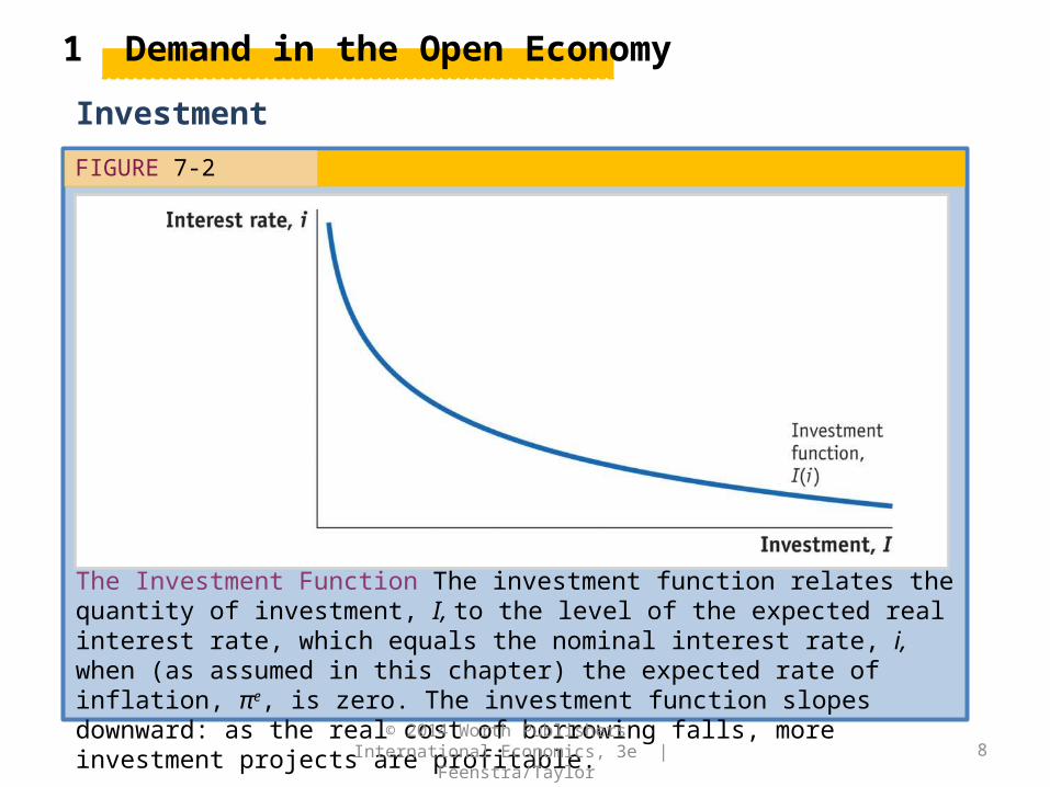
The Investment Function The investment function relates the quantity of investment, I, to the level of the expected real interest rate, which equals the nominal interest rate, i, when (as assumed in this chapter) the expected rate of inflation, πe, is zero. The investment function slopes downward: as the real cost of borrowing falls, more investment projects are profitable.
© 2014 Worth Publishers International Economics, 3e | Feenstra/Taylor
9
1 Demand in the Open Economy
The Government
• Assume that the government collects an amount T of taxes from households and spends an amount G on government consumption.
• We will ignore government transfer programs, such as social security, medical care, or unemployment benefit systems.
• In the unlikely event that G = T exactly, we say that the government has a balanced budget.
• If T > G, the government is said to be running a budget surplus (of size T − G).
• If G > T, a budget deficit (of size G − T or, equivalently, a negative surplus of T − G).
© 2014 Worth Publishers International Economics, 3e | Feenstra/Taylor
10
1 Demand in the Open Economy
The Trade Balance
The Role of the Real Exchange Rate
• When aggregate spending patterns change due to changes in the real exchange rate, this is expenditure switching from foreign purchases to domestic purchases.
• If home’s exchange rate is E, and home and foreign price levels are and * (both fixed in the short run), the real exchange rate q of Home is defined as q = E*/.
o We expect the trade balance of the home country to be an increasing function of the home country’s real exchange rate. As the home country’s real exchange rate rises, it will export more and import less, and the trade balance rises.
© 2014 Worth Publishers International Economics, 3e | Feenstra/Taylor

11
1 Demand in the Open Economy
The Trade Balance
The Role of Income Levelso We expect an increase in home income to be associated
with an increase in home imports and a fall in the home country’s trade balance.
o We expect an increase in rest of the world income to be associated with an increase in home exports and a rise in the home country’s trade balance.
• The trade balance is, therefore, a function of three variables: the real exchange rate, home disposable income, and rest of world disposable income.
),,/(
function Increasing
**
function ng Decreasi
function Increasing
* TYTYPPETBTB
© 2014 Worth Publishers International Economics, 3e | Feenstra/Taylor

Oh! What a Lovely Currency War
In September 2010, the finance minister of Brazil accused other countriesof starting a “currency war” by pursuing policies that made Brazil’scurrency, the real, strengthen against its trading partners, thus harming thecompetitiveness of his country’s exports and pushing Brazil’s trade balancetoward deficit. By 2013 fears about such policies were being expressed bymore and more policy makers around the globe.
HEADLINES
The Curry Trade
In 2009, a dramatic weakening of the pound against the euro sparked an unlikely boom in cross-Channel grocery deliveries. Many Britons living in France used the internet to order groceries from British supermarkets, including everything from bagels to baguettes.
© 2014 Worth Publishers International Economics, 3e | Feenstra/Taylor
12
13
1 Demand in the Open Economy
The Trade Balance
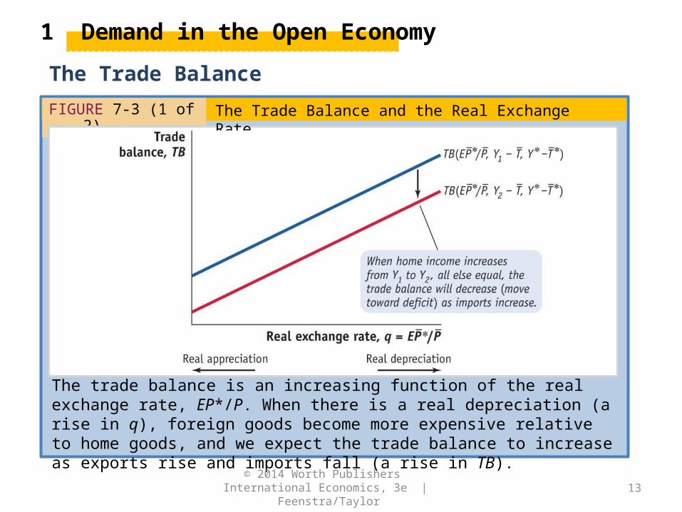
FIGURE 7-3 (1 of 2)
The trade balance is an increasing function of the real exchange rate, EP*/P. When there is a real depreciation (a rise in q), foreign goods become more expensive relative to home goods, and we expect the trade balance to increase as exports rise and imports fall (a rise in TB).
© 2014 Worth Publishers International Economics, 3e | Feenstra/Taylor
The Trade Balance and the Real Exchange Rate
14
1 Demand in the Open Economy
The Trade Balance
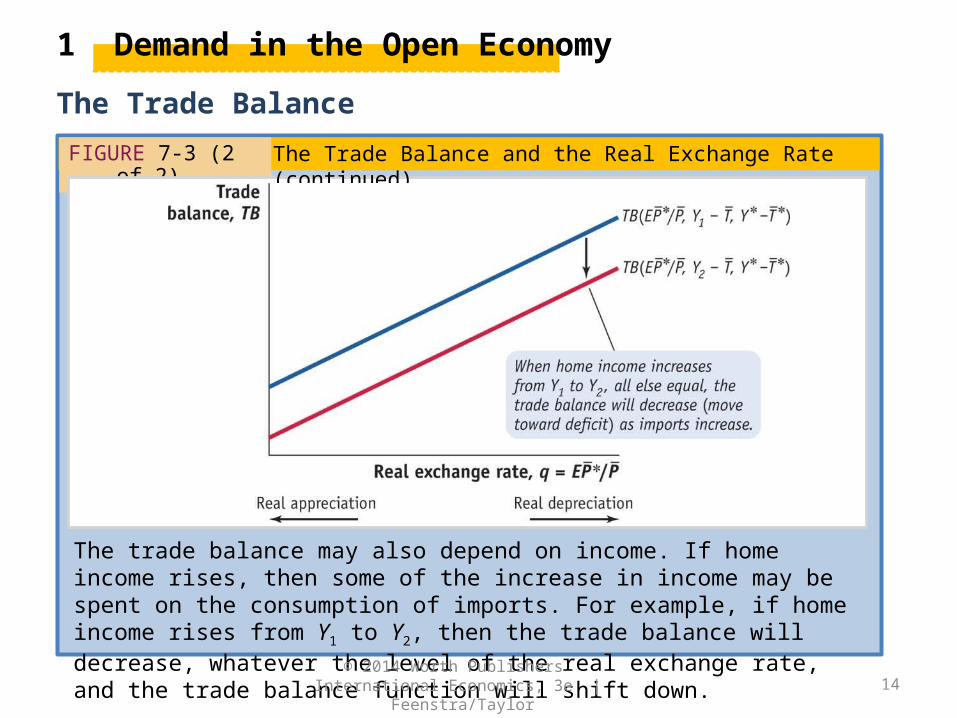
FIGURE 7-3 (2 of 2)
The trade balance may also depend on income. If home income rises, then some of the increase in income may be spent on the consumption of imports. For example, if home income rises from Y1 to Y2, then the trade balance will decrease, whatever the level of the real exchange rate, and the trade balance function will shift down.
© 2014 Worth Publishers International Economics, 3e | Feenstra/Taylor
The Trade Balance and the Real Exchange Rate (continued)
15
1 Demand in the Open Economy
The Trade Balance
Marginal Effects Once More
We refer to MPCF as the marginal propensity to consume foreign imports.
• Let MPCH > 0 be the marginal propensity to consume home goods. By assumption MPC = MPCH + MPCF.
• For example, if MPCF = 0.10 and MPCH = 0.65, then MPC = 0.75; for every extra dollar of disposable income, home consumers spend 75 cents, 10 cents on imported foreign goods and 65 cents on home goods (and they save 25 cents).
© 2014 Worth Publishers International Economics, 3e | Feenstra/Taylor

16
FIGURE 7-4
The Real Exchange Rate and the Trade Balance: United States, 1975-2012 Does the real exchange rate affect the trade balance in the way we have assumed? The data show that the U.S. trade balance is correlated with the U.S. real effective exchange rate index. Because the trade balance also depends on changes in U.S. and rest of the world disposable income (and other factors), it may respond with a lag to changes in the real exchange rate, so the correlation is not perfect (as seen in the years 2002–2007).
APPLICATION
The Trade Balance and the Real Exchange Rate
© 2014 Worth Publishers International Economics, 3e | Feenstra/Taylor

17
APPLICATION
The Trade Balance and the Real Exchange Rate
• A composite or weighted-average measure of the price of goods in all foreign countries relative to the price of U.S. goods is constructed using multilateral measures of real exchange rate movement.
• Applying a trade weight to each bilateral real exchange rate’s percentage change, we obtain the percentage change in home’s multilateral real exchange rate or real effective exchange rate:
%)(in changes rate exchange real bilateral
of average weighted-Trade
2
22
1
11
%)(in change rate exchange effective Real
effective
effective
Trade
Trade
Trade
Trade
Trade
Trade
N
NN
q
q
q
q
q
q
q
q
© 2014 Worth Publishers International Economics, 3e | Feenstra/Taylor

18
Barriers to Expenditure Switching: Pass-Through and the J Curve
1
*
1
*
goods home
priceddollar torelative
goodsforeign of Price
P
P
PE
PE
2
*
goods home
pricedcurrency -local torelative
goodsforeign of Price
P
PE
The price of all foreign-produced goods relative to all home-produced goods is the weighted sum of the relative prices of the two parts of the basket. Hence,
When d is 0, all home goods are priced in local currency and we have our basic model. A 1% rise in E causes a 1% rise in q. There is full pass-through from changes in the nominal exchange rate to changes in the real exchange rate. As d rises, pass-through falls.
2
*
1
*
)1( rate exchange real HomeP
PEd
P
Pd
Trade Dollarization, Distribution, and Pass-Through
© 2014 Worth Publishers International Economics, 3e | Feenstra/Taylor

19
Barriers to Expenditure Switching: Pass-Through and the J Curve
TABLE 7-1 (1 of 2)
The table shows the extent to which the dollar and the euro were used in the invoicing of payments for exports and imports of different countries in the 2002–2004 period. In the United States, for example, 100% of exports are invoiced and paid in U.S. dollars but so, too, are 93% of imports. In Asia, U.S. dollar invoicing is very common, accounting for 48% of Japanese exports and more than 75% of exports and imports in Korea, Malaysia, and Thailand.
Trade Dollarization, Distribution, and Pass-Through
© 2014 Worth Publishers International Economics, 3e | Feenstra/Taylor
Trade Dollarization
20
Barriers to Expenditure Switching: Pass-Through and the J Curve
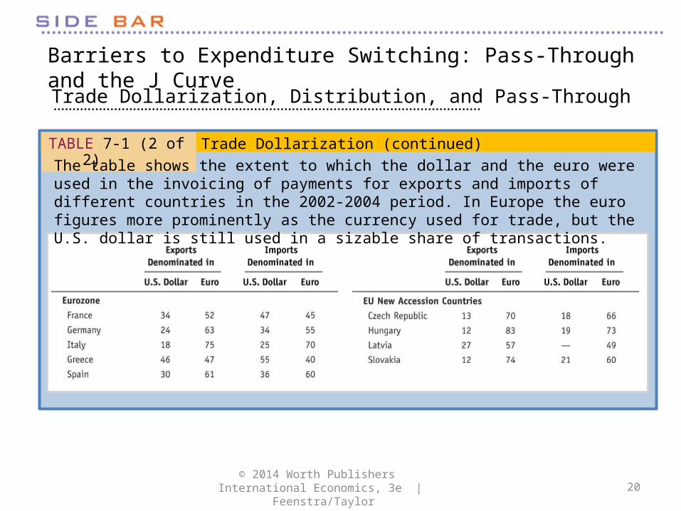
TABLE 7-1 (2 of 2)
The table shows the extent to which the dollar and the euro were used in the invoicing of payments for exports and imports of different countries in the 2002-2004 period. In Europe the euro figures more prominently as the currency used for trade, but the U.S. dollar is still used in a sizable share of transactions.
Trade Dollarization, Distribution, and Pass-Through
© 2014 Worth Publishers International Economics, 3e | Feenstra/Taylor
Trade Dollarization (continued)

21
Barriers to Expenditure Switching: Pass-Through and the J Curve
FIGURE 7-5 (1 of 2)
When prices are sticky and there is a nominal and real depreciation of the home currency, it may take time for the trade balance to move toward surplus. In fact, the initial impact may be toward deficit. If firms and households place orders in advance, then import and export quantities may react sluggishly to changes in the relative price of home and foreign goods. Hence, just after the depreciation, the value of home exports, EX, will be unchanged.
© 2014 Worth Publishers International Economics, 3e | Feenstra/Taylor
The J Curve

22
Barriers to Expenditure Switching: Pass-Through and the J Curve
FIGURE 7-5 (2 of 2)
However, home imports now cost more due to the depreciation. Thus, the value of imports, IM, would actually rise after a depreciation, causing the trade balance TB = EX − IM to fall. Only after some time would exports rise and imports fall, allowing the trade balance to rise relative to its pre-depreciation level. The path traced by the trade balance during this process looks vaguely like a letter J.
© 2014 Worth Publishers International Economics, 3e | Feenstra/Taylor
The J Curve (continued)
23
1 Demand in the Open Economy
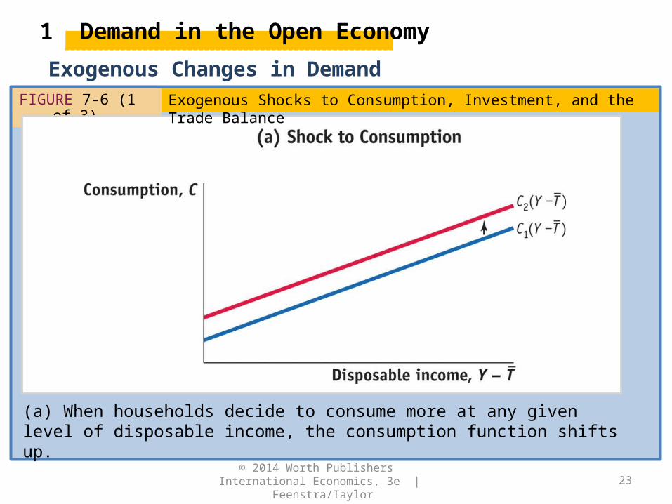
Exogenous Changes in DemandFIGURE 7-6 (1 of 3)
(a) When households decide to consume more at any given level of disposable income, the consumption function shifts up.
© 2014 Worth Publishers International Economics, 3e | Feenstra/Taylor
Exogenous Shocks to Consumption, Investment, and the Trade Balance

24
1 Demand in the Open Economy
Exogenous Changes in DemandFIGURE 7-6 (2 of 3)
(b) When firms decide to invest more at any given level of the interest rate, the investment function shifts right.
© 2014 Worth Publishers International Economics, 3e | Feenstra/Taylor
Exogenous Shocks to Consumption, Investment, and the Trade Balance (continued)

25
1 Demand in the Open Economy
Exogenous Changes in DemandFIGURE 7-6 (3 of 3)
(c) When the trade balance increases at any given level of the real exchange rate, the trade balance function shifts up.
© 2014 Worth Publishers International Economics, 3e | Feenstra/Taylor
Exogenous Shocks to Consumption, Investment, and the Trade Balance (continued)

26
2 Goods Market Equilibrium: The Keynesian Cross
Supply and Demand
Given our assumption that the current account equals the trade balance, gross national income Y equals GDP:
Aggregate demand, or just “demand,” consists of all the possible sources of demand for this supply of output.
Substituting we have
The goods market equilibrium condition is
Supply = GDP Y
Demand = D C I G TB
*** ,,/)()( TYTYPPETBGiITYCD
D
TYTYPPETBGiITYCY *** ,,/)()(
© 2014 Worth Publishers International Economics, 3e | Feenstra/Taylor
(7-1)
27
2 Goods Market Equilibrium: The Keynesian Cross
Determinants of Demand
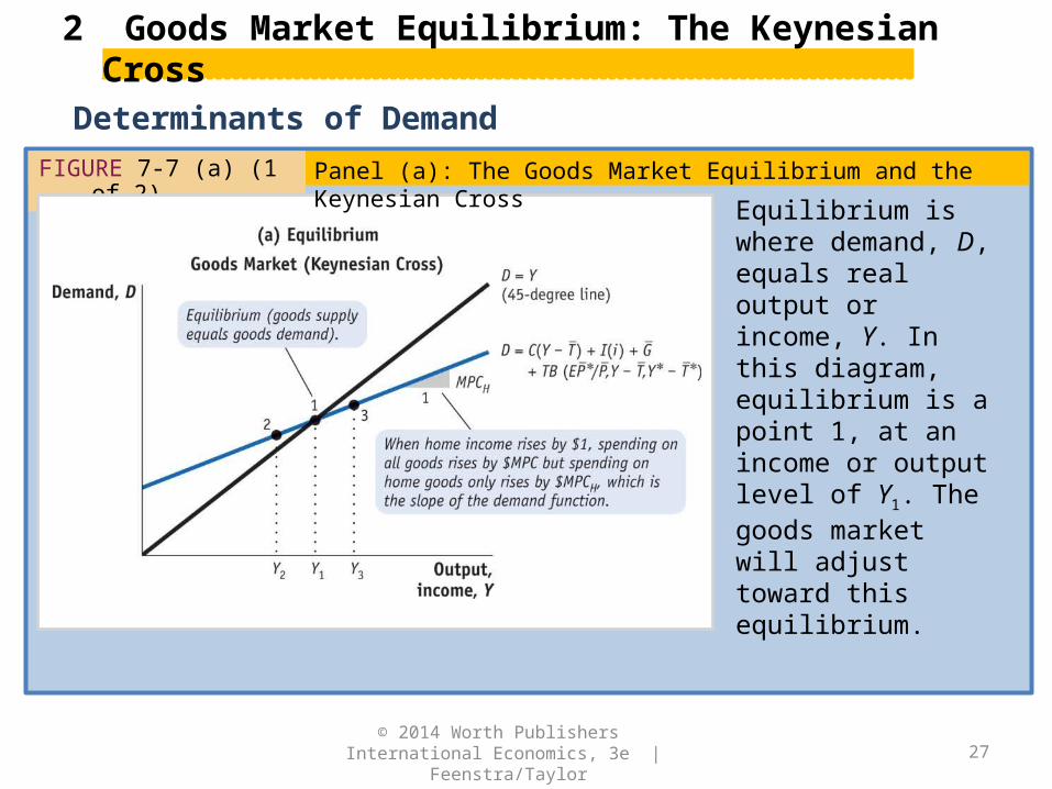
FIGURE 7-7 (a) (1 of 2)
Equilibrium is where demand, D, equals real output or income, Y. In this diagram, equilibrium is a point 1, at an income or output level of Y1. The goods market will adjust toward this equilibrium.
© 2014 Worth Publishers International Economics, 3e | Feenstra/Taylor
Panel (a): The Goods Market Equilibrium and the Keynesian Cross
28
2 Goods Market Equilibrium: The Keynesian Cross
Determinants of Demand
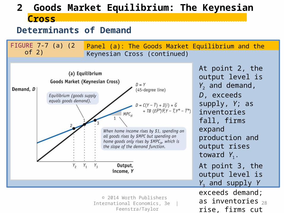
FIGURE 7-7 (a) (2 of 2)
At point 2, the output level is Y2 and demand, D, exceeds supply, Y; as inventories fall, firms expand production and output rises toward Y1.
At point 3, the output level is Y3 and supply Y exceeds demand; as inventories rise, firms cut production and output falls toward Y1.
© 2014 Worth Publishers International Economics, 3e | Feenstra/Taylor
Panel (a): The Goods Market Equilibrium and the Keynesian Cross (continued)
29
2 Goods Market Equilibrium: The Keynesian Cross
Determinants of Demand
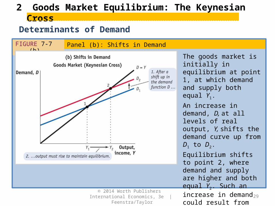
FIGURE 7-7 (b)
The goods market is initially in equilibrium at point 1, at which demand and supply both equal Y1.
An increase in demand, D, at all levels of real output, Y, shifts the demand curve up from D1 to D2.
Equilibrium shifts to point 2, where demand and supply are higher and both equal Y2. Such an increase in demand could result from changes in one or more of the components of demand: C, I, G, or TB.
© 2014 Worth Publishers International Economics, 3e | Feenstra/Taylor
Panel (b): Shifts in Demand
30
2 Goods Market Equilibrium: The Keynesian Cross
Summary
Y
D
D
TB
I
C
P
P
E
i
T
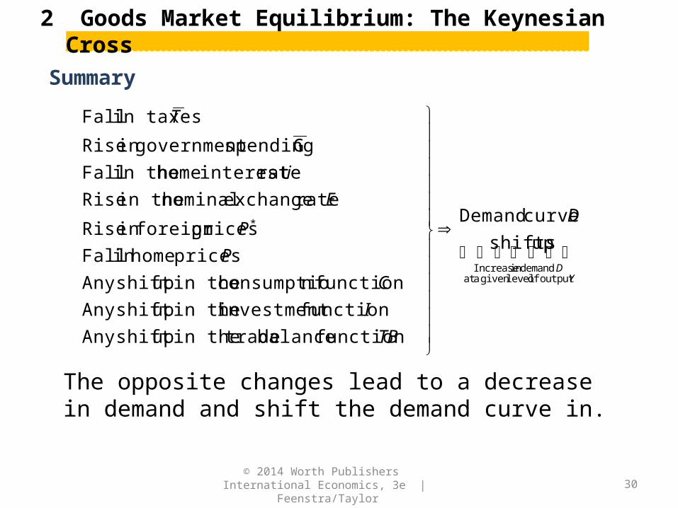
output of levelgiven aat demandin Increase
*
up shifts
curve Demand
function balance tradein the upshift Any
function investment in the upshift Any
function n consumptio in the upshift Any
prices homein Fall
pricesforeign in Rise
rate exchange nominal in the Rise
rateinterest home in the Fall
G spending governmentin Rise
in taxes Fall
The opposite changes lead to a decrease in demand and shift the demand curve in.
© 2014 Worth Publishers International Economics, 3e | Feenstra/Taylor

31
3 Goods and Forex Market Equilibria: Deriving the IS Curve
Equilibrium in Two Markets
• A general equilibrium requires equilibrium in all markets—that is, equilibrium in the goods market, the money market, and the forex market.
• The IS curve shows combinations of output Y and the interest rate i for which the goods and forex markets are in equilibrium.
Forex Market Recap
Uncovered interest parity (UIP) Equation (10-3):
returnforeign Expected
currency domestic theofondepreciati of rate Expected
rateinterest Foreign
*
return Domestic
rateinterest Domestic
1
E
Eii
e
© 2014 Worth Publishers International Economics, 3e | Feenstra/Taylor

32
3 Goods and Forex Market Equilibria: Deriving the IS Curve
Equilibrium in Two Markets
FIGURE 7-8 (1 of 3)
The Keynesian cross is in panel (a), IS curve in panel (b), and forex (FX) market in panel (c).
The economy starts in equilibrium with output, Y1; interest rate, i1; and exchange rate, E1.
Consider the effect of a decrease in the interest rate from i1 to i2, all else equal. In panel (c), a lower interest rate causes a depreciation; equilibrium moves from 1′ to 2′.
© 2014 Worth Publishers International Economics, 3e | Feenstra/Taylor
Deriving the IS Curve
33
3 Goods and Forex Market Equilibria: Deriving the IS Curve
Equilibrium in Two Markets
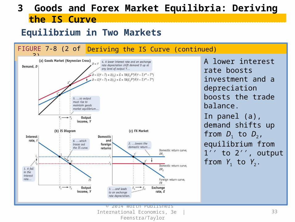
FIGURE 7-8 (2 of 3)
A lower interest rate boosts investment and a depreciation boosts the trade balance.
In panel (a), demand shifts up from D1 to D2, equilibrium from 1′′ to 2′′, output from Y1 to Y2.
© 2014 Worth Publishers International Economics, 3e | Feenstra/Taylor
Deriving the IS Curve (continued)
34
3 Goods and Forex Market Equilibria: Deriving the IS Curve
Equilibrium in Two Markets
FIGURE 7-8 (3 of 3)
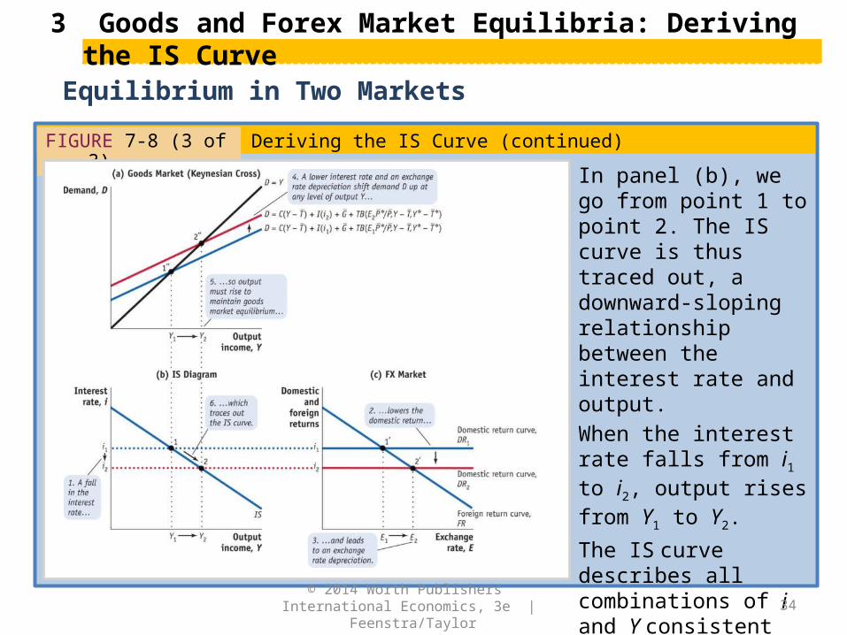
In panel (b), we go from point 1 to point 2. The IS curve is thus traced out, a downward-sloping relationship between the interest rate and output.
When the interest rate falls from i1 to i2, output rises from Y1 to Y2.
The IS curve describes all combinations of i and Y consistent with goods and FX market equilibria in panels (a) and (c).
© 2014 Worth Publishers International Economics, 3e | Feenstra/Taylor
Deriving the IS Curve (continued)
35
3 Goods and Forex Market Equilibria: Deriving the IS Curve
Deriving the IS Curve
One important observation is in order:
• In an open economy, lower interest rates stimulate demand through the traditional closed-economy investment channel and through the trade balance.
• The trade balance effect occurs because lower interest rates cause a nominal depreciation (a real depreciation in the short run), which stimulates external demand.
We have now derived the shape of the IS curve, which describes goods and forex market equilibrium:
• The IS curve is downward-sloping. It illustrates the negative relationship between the interest rate i and output Y.
© 2014 Worth Publishers International Economics, 3e | Feenstra/Taylor
36
3 Goods and Forex Market Equilibria: Deriving the IS Curve
Factors That Shift the IS Curve
FIGURE 7-9 (1 of 2)
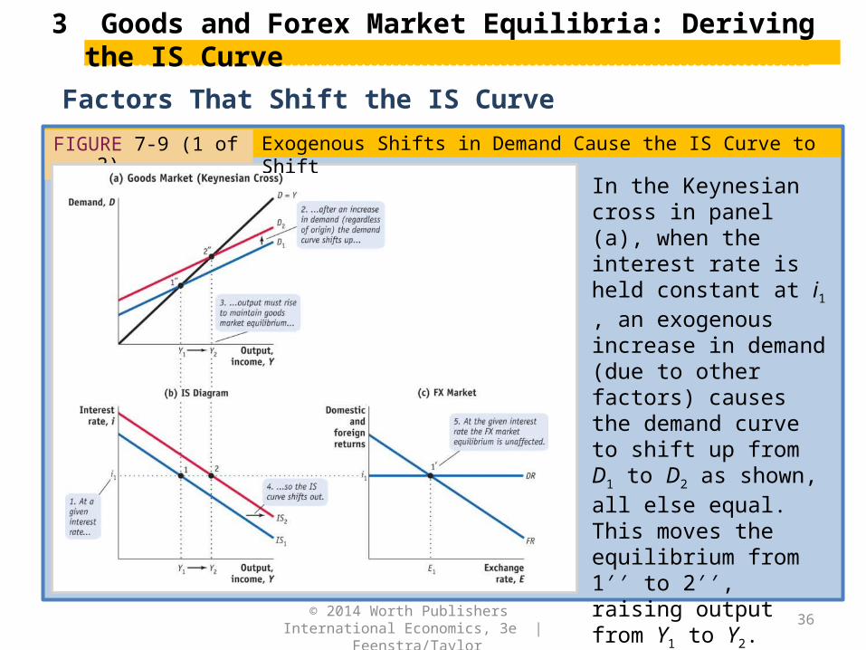
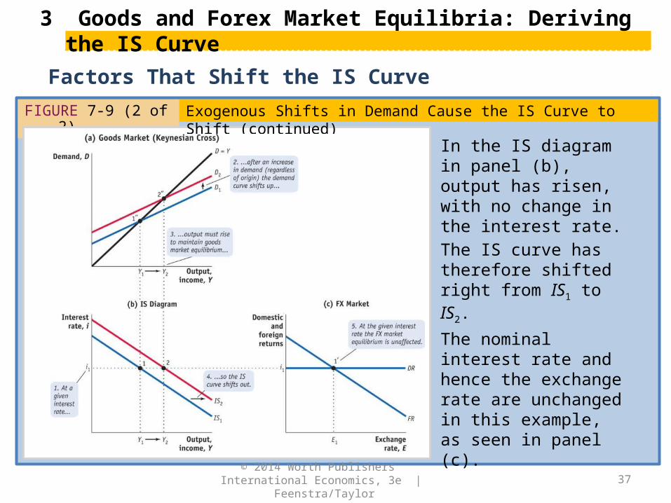
In the Keynesian cross in panel (a), when the interest rate is held constant at i1 , an exogenous increase in demand (due to other factors) causes the demand curve to shift up from D1 to D2 as shown, all else equal. This moves the equilibrium from 1′′ to 2′′, raising output from Y1 to Y2.
© 2014 Worth Publishers International Economics, 3e | Feenstra/Taylor
Exogenous Shifts in Demand Cause the IS Curve to Shift
37
3 Goods and Forex Market Equilibria: Deriving the IS Curve
Factors That Shift the IS Curve
FIGURE 7-9 (2 of 2)
In the IS diagram in panel (b), output has risen, with no change in the interest rate.
The IS curve has therefore shifted right from IS1 to IS2.
The nominal interest rate and hence the exchange rate are unchanged in this example, as seen in panel (c).
© 2014 Worth Publishers International Economics, 3e | Feenstra/Taylor
Exogenous Shifts in Demand Cause the IS Curve to Shift (continued)

38
3 Goods and Forex Market Equilibria: Deriving the IS Curve
Summing Up the IS Curve
IS IS(G,T , i*,Ee, P*,P)
i
Y
i
YD
e
*
D
TB
I
C
P
P
E
i
G
T
rateinterest homegiven aat
output mequilibriuin Increase
rateinterest homegiven aat and
output of levelany at demandin Increase
*
right shifts
curve IS
up shifts
curve Demand
function balance tradein the upshift Any
function investment in the upshift Any
function n consumptio in the upshift Any
prices homein Fall
pricesforeign in Rise
rate exchange expected futurein Rise
rateinterest foreign in Rise
spending governmentin Rise
in taxes Fall
Factors That Shift the IS Curve
The opposite changes lead to a decrease in demand and shift the demand curve down and the IS curve to the left.
© 2014 Worth Publishers International Economics, 3e | Feenstra/Taylor
39
4 Money Market Equilibrium: Deriving the LM Curve
Money Market Recap
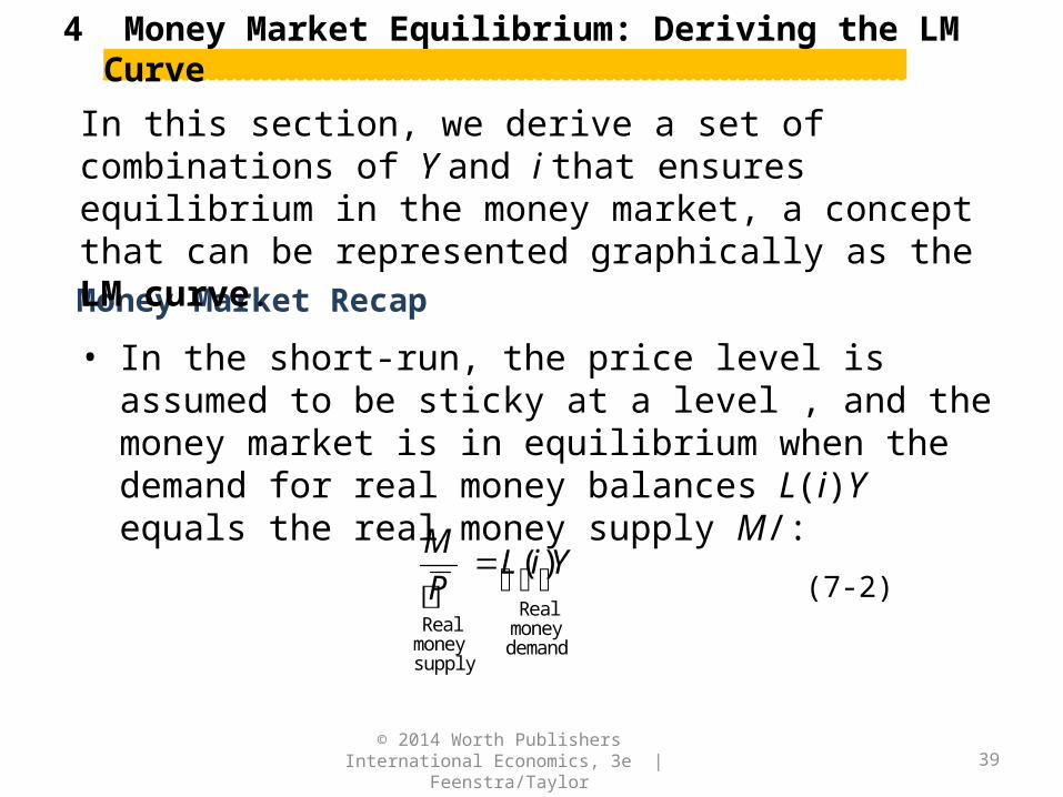
In this section, we derive a set of combinations of Y and i that ensures equilibrium in the money market, a concept that can be represented graphically as the LM curve.
demandmoneyReal
supplymoneyReal
)( YiLP
M
• In the short-run, the price level is assumed to be sticky at a level , and the money market is in equilibrium when the demand for real money balances L(i)Y equals the real money supply M/:
(7-2)
© 2014 Worth Publishers International Economics, 3e | Feenstra/Taylor

40
4 Money Market Equilibrium: Deriving the LM Curve
Deriving the LM CurveFIGURE 7-10 (1 of 2)
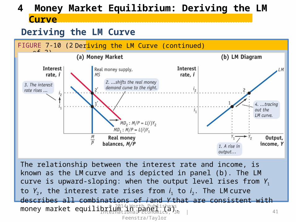
If there is an increase in real income or output from Y1 to Y2 in panel (b), the effect in the money market in panel (a) is to shift the demand for real money balances to the right, all else equal. If the real supply of money, MS, is held fixed at M/, then the interest rate rises from i1 to i2 and money market equilibrium moves from point 1′ to point 2′.
© 2014 Worth Publishers International Economics, 3e | Feenstra/Taylor
Deriving the LM Curve
41
4 Money Market Equilibrium: Deriving the LM Curve
Deriving the LM CurveFIGURE 7-10 (2 of 2)
The relationship between the interest rate and income, is known as the LM curve and is depicted in panel (b). The LM curve is upward-sloping: when the output level rises from Y1 to Y2, the interest rate rises from i1 to i2. The LM curve describes all combinations of i and Y that are consistent with money market equilibrium in panel (a).
© 2014 Worth Publishers International Economics, 3e | Feenstra/Taylor
Deriving the LM Curve (continued)
42
4 Money Market Equilibrium: Deriving the LM Curve
Factors That Shift the LM CurveFIGURE 7-11 (1 of 2)
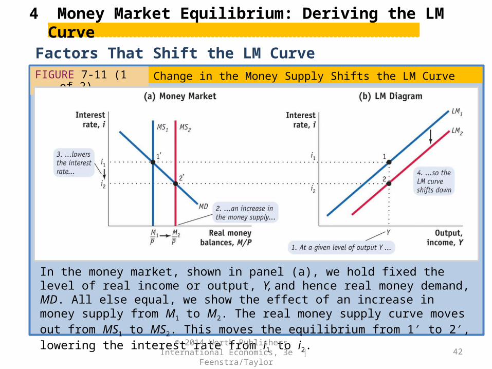
In the money market, shown in panel (a), we hold fixed the level of real income or output, Y, and hence real money demand, MD. All else equal, we show the effect of an increase in money supply from M1 to M2. The real money supply curve moves out from MS1 to MS2. This moves the equilibrium from 1′ to 2′, lowering the interest rate from i1 to i2.
© 2014 Worth Publishers International Economics, 3e | Feenstra/Taylor
Change in the Money Supply Shifts the LM Curve

43
4 Money Market Equilibrium: Deriving the LM Curve
Factors That Shift the LM CurveFIGURE 7-11 (2 of 2)
In the LM diagram, shown in panel (b), the interest rate has fallen, with no change in the level of income or output, so the economy moves from point 1 to point 2.
The LM curve has therefore shifted down from LM1 to LM2.
© 2014 Worth Publishers International Economics, 3e | Feenstra/Taylor
Change in the Money Supply Shifts the LM Curve (continued)
44
4 Money Market Equilibrium: Deriving the LM Curve
Summing Up the LM Curve
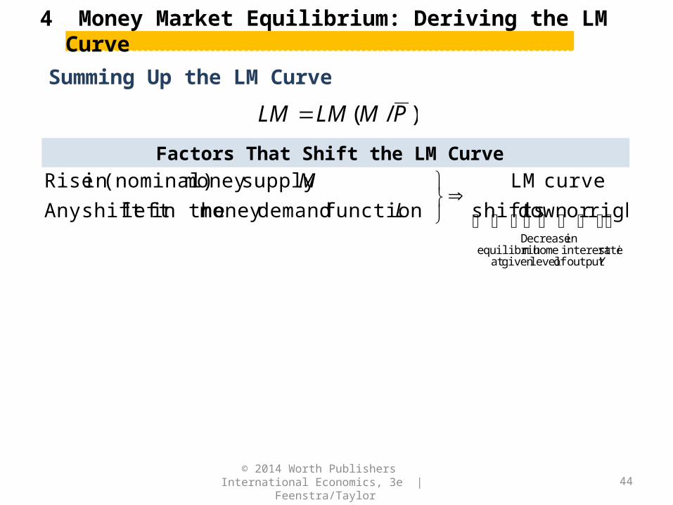
LM LM (M / P )
Yi
L
M
output of levelgiven at rateinterest home mequilibriu
in Decrease
rightor down shifts
curve LM
function demandmoney in theleft shift Any
supply money (nominal)in Rise
Factors That Shift the LM Curve
© 2014 Worth Publishers International Economics, 3e | Feenstra/Taylor

45
5 The Short-Run IS-LM-FX Model of an Open Economy
FIGURE 7-12 (1 of 2)
In panel (a), the IS and LM curves are both drawn. The goods and forex markets are in equilibrium when the economy is on the IS curve. The money market is in equilibrium when the economy is on the LM curve. Both markets are in equilibrium if and only if the economy is at point 1, the unique point of intersection of IS and LM.
© 2014 Worth Publishers International Economics, 3e | Feenstra/Taylor
Equilibrium in the IS-LM-FX Model
46
FIGURE 7-12 (2 of 2)
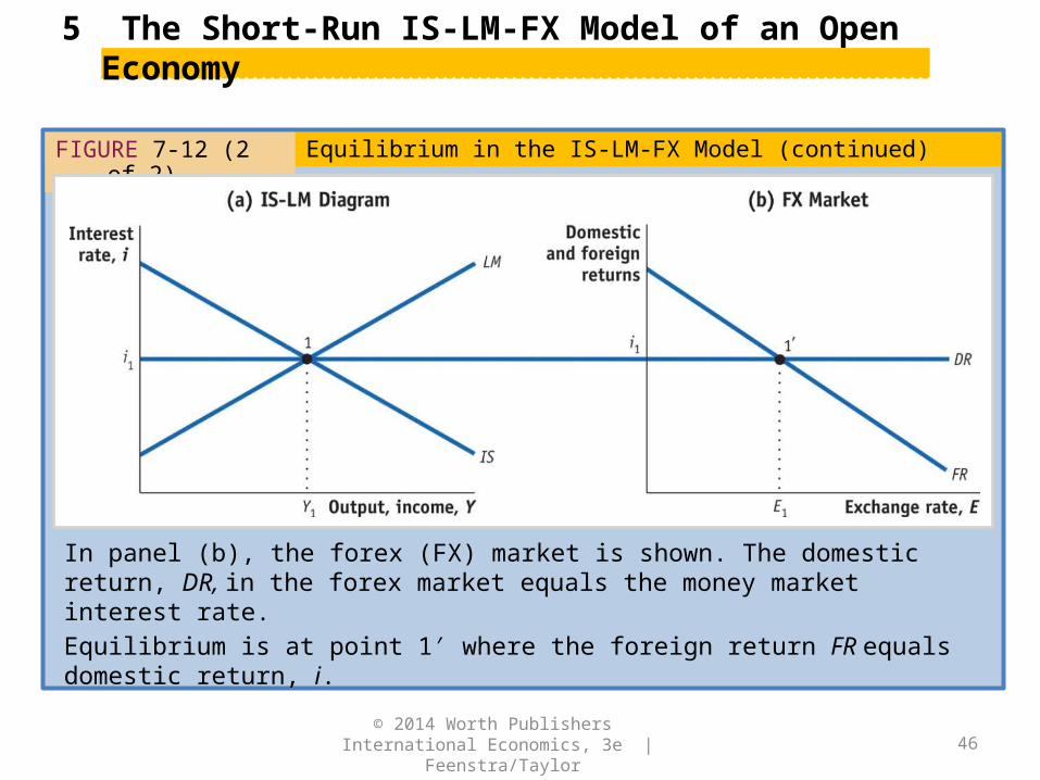
In panel (b), the forex (FX) market is shown. The domestic return, DR, in the forex market equals the money market interest rate.
Equilibrium is at point 1′ where the foreign return FR equals domestic return, i.
5 The Short-Run IS-LM-FX Model of an Open Economy
© 2014 Worth Publishers International Economics, 3e | Feenstra/Taylor
Equilibrium in the IS-LM-FX Model (continued)
47
Macroeconomic Policies in the Short Run
5 The Short-Run IS-LM-FX Model of an Open Economy
We focus on the two main policy actions: changes in monetary policy, through changes in the money supply, and changes in fiscal policy, involving changes in government spending or taxes.
The key assumptions of this section are as follows:
• The economy begins in a state of long-run equilibrium. We then consider policy changes in the home economy, assuming that conditions in the foreign economy (i.e., the rest of the world) are unchanged.
• The home economy is subject to the usual short-run assumption of a sticky price level at home and abroad.
• Furthermore, we assume that the forex market operates freely and unrestricted by capital controls and that the exchange rate is determined by market forces.
© 2014 Worth Publishers International Economics, 3e | Feenstra/Taylor
48
Monetary Policy Under Floating Exchange Rates
FIGURE 7-13 (1 of 2)
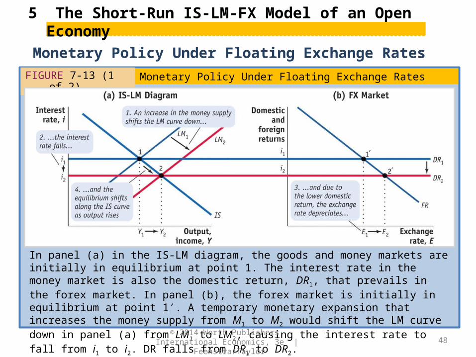
In panel (a) in the IS-LM diagram, the goods and money markets are initially in equilibrium at point 1. The interest rate in the money market is also the domestic return, DR1, that prevails in the forex market. In panel (b), the forex market is initially in equilibrium at point 1′. A temporary monetary expansion that increases the money supply from M1 to M2 would shift the LM curve down in panel (a) from LM1 to LM2, causing the interest rate to fall from i1 to i2. DR falls from DR1 to DR2.
5 The Short-Run IS-LM-FX Model of an Open Economy
© 2014 Worth Publishers International Economics, 3e | Feenstra/Taylor
Monetary Policy Under Floating Exchange Rates

49
Monetary Policy Under Floating Exchange Rates
FIGURE 7-13 (2 of 2)
In panel (b), the lower interest rate implies that the exchange rate must depreciate, rising from E1 to E2. As the interest rate falls (increasing investment, I) and the exchange rate depreciates (increasing the trade balance), demand increases, which corresponds to the move down the IS curve from point 1 to point 2. Output expands from Y1 to Y2. The new equilibrium corresponds to points 2 and 2′.
5 The Short-Run IS-LM-FX Model of an Open Economy
© 2014 Worth Publishers International Economics, 3e | Feenstra/Taylor
Monetary Policy Under Floating Exchange Rates (continued)
50
Monetary Policy Under Floating Exchange Rates
5 The Short-Run IS-LM-FX Model of an Open Economy
To sum up:
• A temporary monetary expansion under floating exchange rates is effective in combating economic downturns by boosting output.
• It raises output at home, lowers the interest rate, and causes a depreciation of the exchange rate. What happens to the trade balance cannot be predicted with certainty.
© 2014 Worth Publishers International Economics, 3e | Feenstra/Taylor
51
Monetary Policy Under Fixed Exchange Rates
FIGURE 7-14 (1 of 2)
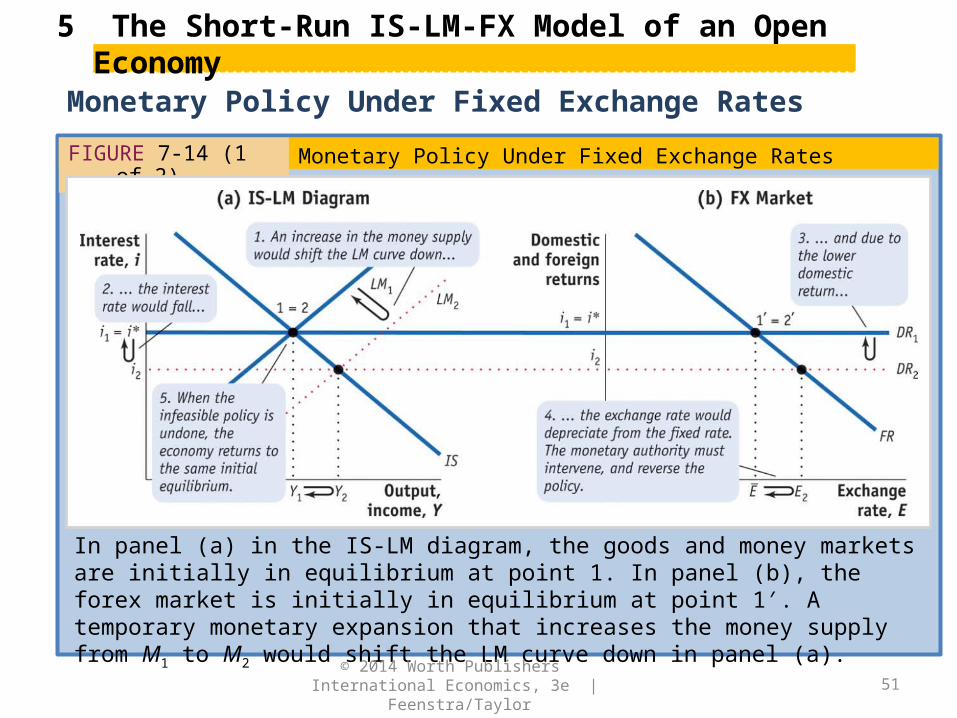
In panel (a) in the IS-LM diagram, the goods and money markets are initially in equilibrium at point 1. In panel (b), the forex market is initially in equilibrium at point 1′. A temporary monetary expansion that increases the money supply from M1 to M2 would shift the LM curve down in panel (a).
5 The Short-Run IS-LM-FX Model of an Open Economy
© 2014 Worth Publishers International Economics, 3e | Feenstra/Taylor
Monetary Policy Under Fixed Exchange Rates

52
Monetary Policy Under Fixed Exchange Rates
FIGURE 7-14 (2 of 2)
5 The Short-Run IS-LM-FX Model of an Open Economy
In panel (b), the lower interest rate implies that the exchange rate must depreciate, rising from E1 to E2. This depreciation is inconsistent with the pegged exchange rate, so the policy makers cannot move LM in this way, leaving the money supply equal to M1. Implication: under a fixed exchange rate, autonomous monetary policy is not an option.
⎯ ⎯
© 2014 Worth Publishers International Economics, 3e | Feenstra/Taylor
Monetary Policy Under Fixed Exchange Rates (continued)

53
Monetary Policy Under Fixed Exchange Rates
5 The Short-Run IS-LM-FX Model of an Open Economy
To sum up:
• Monetary policy under fixed exchange rates is impossible to undertake. Fixing the exchange rate means giving up monetary policy autonomy.
• Countries cannot simultaneously allow capital mobility, maintain fixed exchange rates, and pursue an autonomous monetary policy.
© 2014 Worth Publishers International Economics, 3e | Feenstra/Taylor
54
Fiscal Policy Under Floating Exchange RatesFIGURE 7-15 (1 of 3)
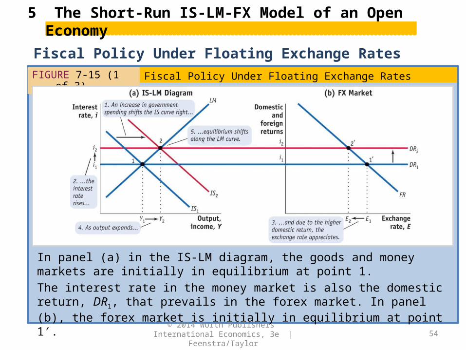
In panel (a) in the IS-LM diagram, the goods and money markets are initially in equilibrium at point 1.
The interest rate in the money market is also the domestic return, DR1, that prevails in the forex market. In panel (b), the forex market is initially in equilibrium at point 1′.
5 The Short-Run IS-LM-FX Model of an Open Economy
© 2014 Worth Publishers International Economics, 3e | Feenstra/Taylor
Fiscal Policy Under Floating Exchange Rates

55
Fiscal Policy Under Floating Exchange Rates
FIGURE 7-15 (2 of 3)
A temporary fiscal expansion that increases government spending from G1 to G2 would shift the IS curve to the right in panel (a) from IS1 to IS2, causing the interest rate to rise from i1 to i2. The domestic return shifts up from DR1 to DR2.
5 The Short-Run IS-LM-FX Model of an Open Economy
© 2014 Worth Publishers International Economics, 3e | Feenstra/Taylor
Fiscal Policy Under Floating Exchange Rates (continued)
56
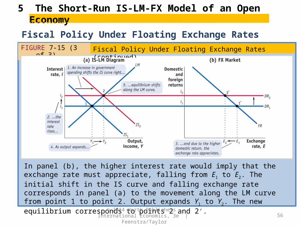
Fiscal Policy Under Floating Exchange RatesFIGURE 7-15 (3 of 3)
In panel (b), the higher interest rate would imply that the exchange rate must appreciate, falling from E1 to E2. The initial shift in the IS curve and falling exchange rate corresponds in panel (a) to the movement along the LM curve from point 1 to point 2. Output expands Y1 to Y2. The new equilibrium corresponds to points 2 and 2′.
5 The Short-Run IS-LM-FX Model of an Open Economy
© 2014 Worth Publishers International Economics, 3e | Feenstra/Taylor
Fiscal Policy Under Floating Exchange Rates (continued)

57
Fiscal Policy Under Floating Exchange Rates
5 The Short-Run IS-LM-FX Model of an Open Economy
• As the interest rate rises (decreasing investment, I) and the exchange rate appreciates (decreasing the trade balance), demand falls.
• This impact of fiscal expansion is often referred to as crowding out. That is, the increase in government spending is offset by a decline in private spending.
• Thus, in an open economy, fiscal expansion crowds out investment (by raising the interest rate) and decreases net exports (by causing the exchange rate to appreciate).
• Over time, it limits the rise in output to less than the increase in government spending.
© 2014 Worth Publishers International Economics, 3e | Feenstra/Taylor
58
Fiscal Policy Under Floating Exchange Rates
5 The Short-Run IS-LM-FX Model of an Open Economy
To sum up:
• An expansion of fiscal policy under floating exchange rates might be temporarily effective.
• It raises output at home, raises the interest rate, causes an appreciation of the exchange rate, and decreases the trade balance.
• It indirectly leads to crowding out of investment and exports, and thus limits the rise in output to less than an increase in government spending.
• A temporary contraction of fiscal policy has opposite effects.
© 2014 Worth Publishers International Economics, 3e | Feenstra/Taylor

59
Fiscal Policy Under Fixed Exchange Rates
FIGURE 7-16 (1 of 3)
In panel (a) in the IS-LM diagram, the goods and money markets are initially in equilibrium at point 1. The interest rate in the money market is also the domestic return, DR1, that prevails in the forex market. In panel (b), the forex market is initially in equilibrium at point 1′.
5 The Short-Run IS-LM-FX Model of an Open Economy
© 2014 Worth Publishers International Economics, 3e | Feenstra/Taylor
Fiscal Policy Under Fixed Exchange Rates

60
Fiscal Policy Under Fixed Exchange Rates
FIGURE 7-16 (2 of 3)
A temporary fiscal expansion on its own increases government spending from G1 to G2
and would shift the IS curve to the right in panel (a) from IS1 to IS2, causing the interest rate to rise from i1 to i2.
The domestic return would then rise from DR1 to DR2.
5 The Short-Run IS-LM-FX Model of an Open Economy
⎯ ⎯
© 2014 Worth Publishers International Economics, 3e | Feenstra/Taylor
Fiscal Policy Under Fixed Exchange Rates (continued)

61
Fiscal Policy Under Fixed Exchange Rates
FIGURE 7-16 (3 of 3)
In panel (b), the higher interest rate would imply that the exchange rate must appreciate, falling from E to E2. To maintain the peg, the monetary authority must intervene, shifting the LM curve down, from LM1 to LM2. The fiscal expansion thus prompts a monetary expansion. In the end, the interest rate and exchange rate are left unchanged, and output expands dramatically from Y1 to Y2. The new equilibrium is at to points 2 and 2′.
5 The Short-Run IS-LM-FX Model of an Open Economy
⎯
© 2014 Worth Publishers International Economics, 3e | Feenstra/Taylor
Fiscal Policy Under Fixed Exchange Rates (continued)
62
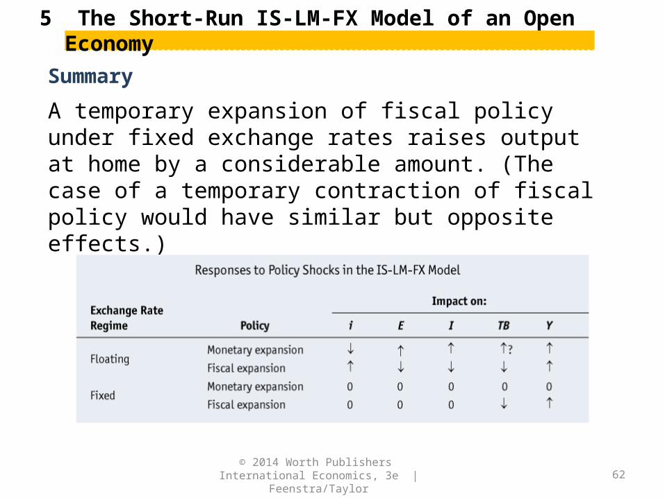
Summary
5 The Short-Run IS-LM-FX Model of an Open Economy
A temporary expansion of fiscal policy under fixed exchange rates raises output at home by a considerable amount. (The case of a temporary contraction of fiscal policy would have similar but opposite effects.)
© 2014 Worth Publishers International Economics, 3e | Feenstra/Taylor

63
Authorities can use changes in policies to try to keep the economy at or near its full-employment level of output. This is the essence of stabilization policy.
• If the economy is hit by a temporary adverse shock, policy makers could use expansionary monetary and fiscal policies to prevent a deep recession.
• Conversely, if the economy is pushed by a shock above its full employment level of output, contractionary policies could tame the boom.
6 Stabilization Policy
© 2014 Worth Publishers International Economics, 3e | Feenstra/Taylor
64
The Right Time for Austerity?
APPLICATION
© 2014 Worth Publishers International Economics, 3e | Feenstra/Taylor
After the global financial crisis, many observers predicted economic difficulties for Eastern Europe in the short run. We use our analytical tools to look at two opposite cases: Poland, which fared well, and Latvia, which did not.
• Demand for Poland’s and Latvia’s exports declined with the contraction of foreign output, this along with negative shocks to consumption and investment can be represented as a leftward shift of the IS curve to the right.
• The policy responses differed in each country, illustrating the contrasts between fixed and floating regimes.

65
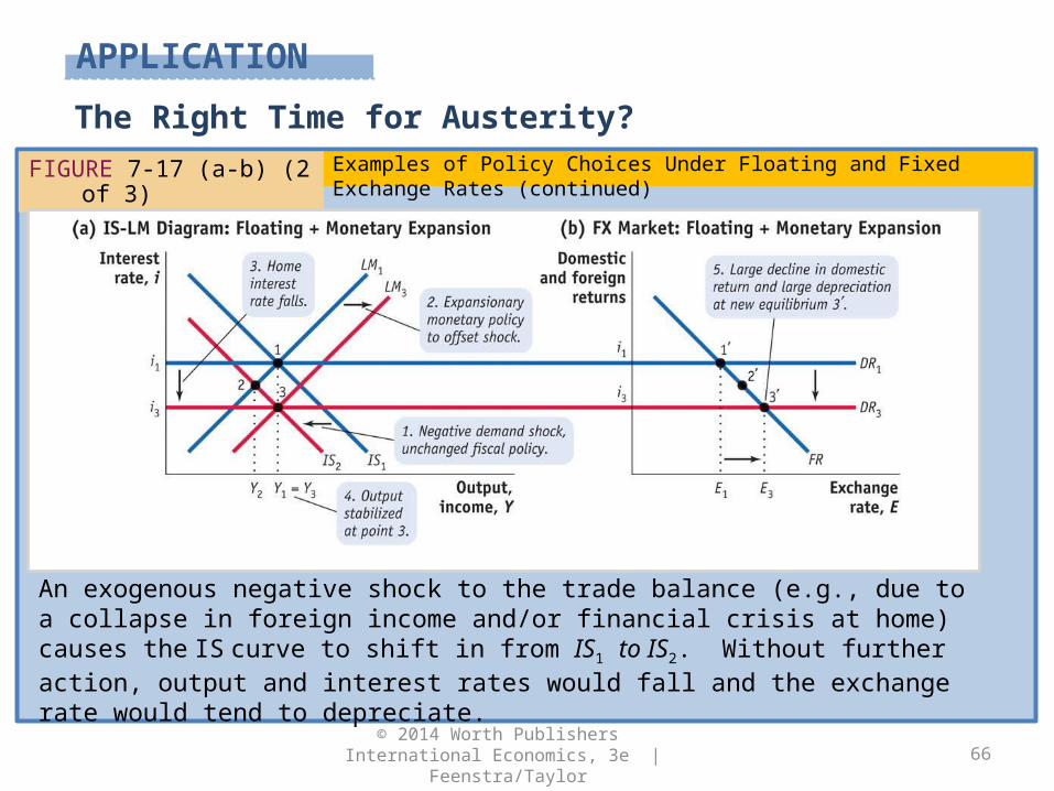
The Right Time for Austerity?FIGURE 7-17(a-b) (1 of 3)
In panels (a) and (b), we explore what happens when the central bank can stabilize output by responding with a monetary policy expansion. In panel (a) in the IS-LM diagram, the goods and money markets are initially in equilibrium at point 1. The interest rate in the money market is also the domestic return, DR1, that prevails in the forex market. In panel (b), the forex market is initially in equilibrium at point 1′.
APPLICATION
© 2014 Worth Publishers International Economics, 3e | Feenstra/Taylor
Examples of Policy Choices Under Floating and Fixed Exchange Rates
66
FIGURE 7-17 (a-b) (2 of 3)
An exogenous negative shock to the trade balance (e.g., due to a collapse in foreign income and/or financial crisis at home) causes the IS curve to shift in from IS1 to IS2. Without further action, output and interest rates would fall and the exchange rate would tend to depreciate.
APPLICATION
© 2014 Worth Publishers International Economics, 3e | Feenstra/Taylor
The Right Time for Austerity?Examples of Policy Choices Under Floating and Fixed Exchange Rates (continued)

67
FIGURE 7-17 (a-b) (3 of 3)
With a floating exchange rate, the central bank can stabilize output at its former level by responding with a monetary policy expansion, increasing the money supply from M1 to M2. This causes the LM curve to shift down from LM1 to LM2.The new equilibrium corresponds to points 3 and 3′. Output is now stabilized at the original level Y1. The interest rate falls further. The exchange rate depreciates all the way from E1 to E2.
APPLICATION
© 2014 Worth Publishers International Economics, 3e | Feenstra/Taylor
The Right Time for Austerity?
Examples of Policy Choices Under Floating and Fixed Exchange Rates (continued)

68
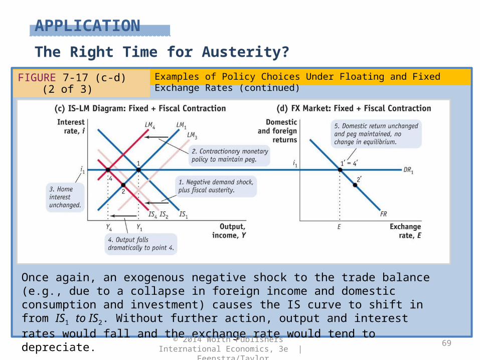
FIGURE 7-17 (c-d) (1 of 3)
In panels (c) and (d) we explore what happens when the exchange rate is fixed and the government pursues austerity and cuts government spending G.
APPLICATION
© 2014 Worth Publishers International Economics, 3e | Feenstra/Taylor
The Right Time for Austerity?
Examples of Policy Choices Under Floating and Fixed Exchange Rates (continued)
69
FIGURE 7-17 (c-d) (2 of 3)
Once again, an exogenous negative shock to the trade balance (e.g., due to a collapse in foreign income and domestic consumption and investment) causes the IS curve to shift in from IS1 to IS2. Without further action, output and interest rates would fall and the exchange rate would tend to depreciate.
APPLICATION
© 2014 Worth Publishers International Economics, 3e | Feenstra/Taylor
The Right Time for Austerity?
Examples of Policy Choices Under Floating and Fixed Exchange Rates (continued)

70
FIGURE 7-17 (c-d) (3 of 3)
With austerity policy, government cuts spending G and the IS shifts leftward more to IS4. If the central bank does nothing, the home interest rate would fall and the exchange rate would depreciate at point 2 and 2′. To maintain the peg, as dictated by the trilemma, the home central bank must engage in contractionary monetary policy, decreasing the money supply and causing the LM curve to shift in all the way from LM1 to LM4.
APPLICATION
© 2014 Worth Publishers International Economics, 3e | Feenstra/Taylor
The Right Time for Austerity?
Examples of Policy Choices Under Floating and Fixed Exchange Rates (continued)
Poland Is Not LatviaHEADLINES
© 2014 Worth Publishers International Economics, 3e | Feenstra/Taylor 71
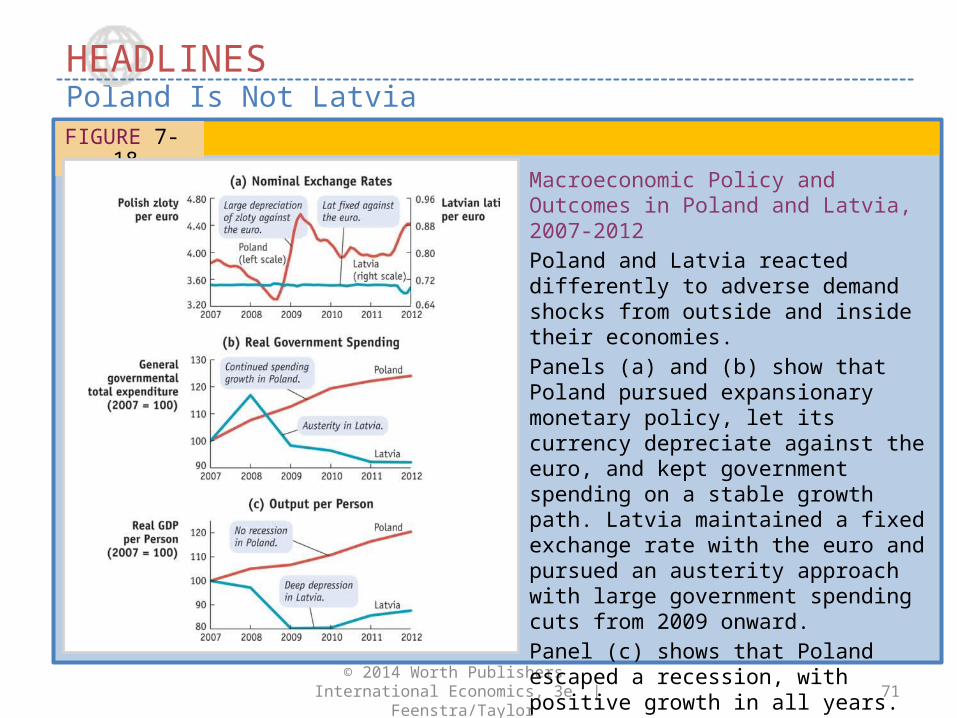
FIGURE 7-18
Macroeconomic Policy and Outcomes in Poland and Latvia, 2007-2012
Poland and Latvia reacted differently to adverse demand shocks from outside and inside their economies.
Panels (a) and (b) show that Poland pursued expansionary monetary policy, let its currency depreciate against the euro, and kept government spending on a stable growth path. Latvia maintained a fixed exchange rate with the euro and pursued an austerity approach with large government spending cuts from 2009 onward.
Panel (c) shows that Poland escaped a recession, with positive growth in all years. In contrast, Latvia fell into a deep depression, and real GDP per capita fell 20% from its 2007 peak.

72
Policy Constraints A fixed exchange rate rules out use of monetary policy. Other firm monetary or fiscal policy rules, such as interest rate or balanced-budget rules, limit on policy.
Incomplete Information and the Inside Lag It takes weeks or months for policy makers to understand the state of the economy today. Then, it takes time to formulate a policy response (the lag between shock and policy actions is called the inside lag).
Policy Response and the Outside Lag It takes time for whatever policies are enacted to have any effect on the economy (the lag between policy actions and effects is called the outside lag).
6 Stabilization Policy
Problems in Policy Design and Implementation
© 2014 Worth Publishers International Economics, 3e | Feenstra/Taylor

73
Long-Horizon Plans If the private sector understands that a policy change is temporary, there may be reasons not to change expenditures. A temporary real appreciation may also have little effect on whether a firm can profit in the long run from sales in the foreign market.
Weak Links from the Nominal Exchange Rate to the Real Exchange Rate Changes in the nominal exchange rate may not translate into changes in the real exchange rate for some goods and services.
Pegged Currency Blocs Exchange rate arrangements in some countries may be characterized by a mix of floating and fixed exchange rate systems with different trading partners.
6 Stabilization Policy
Problems in Policy Design and Implementation
© 2014 Worth Publishers International Economics, 3e | Feenstra/Taylor

74
Weak Links from the Real Exchange Rate to the Trade Balance
Changes in the real exchange rate may not lead to changes in the trade balance. The reasons for this weak linkage include transaction costs in trade, and the J curve effects.
• These effects may cause expenditure switching to be a nonlinear phenomenon: it will be weak at first and then much stronger as the real exchange rate change grows larger.
• For example: Prices of BMWs in the U.S. barely change in response to changes in the dollar-euro exchange rate.
6 Stabilization Policy
Problems in Policy Design and Implementation
© 2014 Worth Publishers International Economics, 3e | Feenstra/Taylor

75
Macroeconomic Policies in the Liquidity Trap
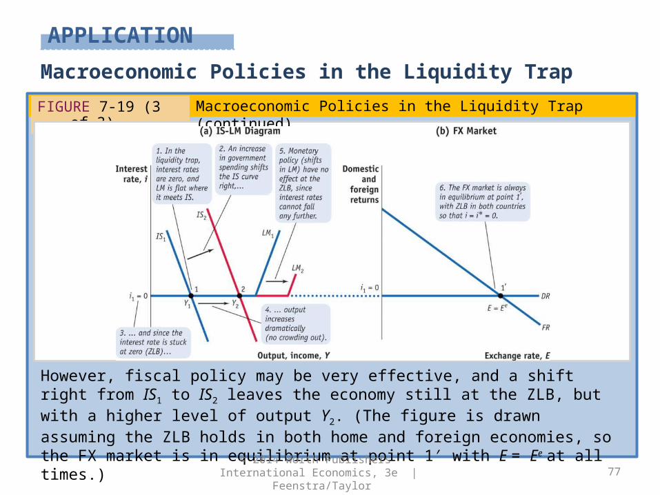
FIGURE 7-19 (1 of 3)
APPLICATION
After a severe negative shock to demand, the IS curve may move very far to the left (IS1). The nominal interest rate may then fall all the way to the zero lower bound (ZLB), with IS1 intersecting the flat portion of the LM1 curve at point 1, in panel (a). Output is depressed at a level Y1.
© 2014 Worth Publishers International Economics, 3e | Feenstra/Taylor
Macroeconomic Policies in the Liquidity Trap

76
Macroeconomic Policies in the Liquidity Trap
FIGURE 7-19 (2 of 3)
APPLICATION
In this scenario, monetary policy is impotent because expansionary monetary policy (e.g., a rightward shift from LM1 to LM2) cannot lower the interest rate any further.
© 2014 Worth Publishers International Economics, 3e | Feenstra/Taylor
Macroeconomic Policies in the Liquidity Trap (continued)
77
Macroeconomic Policies in the Liquidity Trap
FIGURE 7-19 (3 of 3)
However, fiscal policy may be very effective, and a shift right from IS1 to IS2 leaves the economy still at the ZLB, but with a higher level of output Y2. (The figure is drawn assuming the ZLB holds in both home and foreign economies, so the FX market is in equilibrium at point 1′ with E = Ee at all times.)
APPLICATION
© 2014 Worth Publishers International Economics, 3e | Feenstra/Taylor
Macroeconomic Policies in the Liquidity Trap (continued)

78
Macroeconomic Policies in the Liquidity Trap
FIGURE 7-20 (1 of 3)
In the U.S. economic slump of 2008-2010, output had fallen 6% below the estimate of potential level of GDP by the first quarter of 2009, as seen in panel (a). This was the worst U.S. recession since the 1930s. Policy responses included automatic fiscal expansion (increases in spending and reductions in taxes), plus an additional discretionary stimulus.
APPLICATION
© 2014 Worth Publishers International Economics, 3e | Feenstra/Taylor
U.S. Fiscal Policy in the Great Recession: Didn’t Work or Wasn’t Tried?

79
Macroeconomic Policies in the Liquidity Trap
FIGURE 7-20 (2 of 3)
The tax part of the stimulus appeared to do very little: significant reductions in taxes seen in panel (b) were insufficient to prop up consumption expenditure, as seen in panel (a), as consumers saved the extra disposable income.
APPLICATION
© 2014 Worth Publishers International Economics, 3e | Feenstra/Taylor
U.S. Fiscal Policy in the Great Recession: Didn’t Work or Wasn’t Tried? (continued)

80
Macroeconomic Policies in the Liquidity Trap
FIGURE 7-20 (3 of 3)
And on the government spending side there was no stimulus at all in the aggregate: increases in federal government expenditure were fully offset by cuts in state and local government expenditure, as seen in panel (b).
APPLICATION
© 2014 Worth Publishers International Economics, 3e | Feenstra/Taylor
U.S. Fiscal Policy in the Great Recession: Didn’t Work or Wasn’t Tried? (continued)

81
Macroeconomic Policies in the Liquidity Trap
APPLICATION
The aggregate U.S. fiscal stimulus had four major weaknesses:
1. It was rolled out too slowly, due to policy lags.
2. The overall package was too small, given the magnitude of the decline in aggregate demand.
3. The government spending portion of the stimulus, for which positive expenditure effects were certain, ended up being close to zero, due to state and local cuts.
4. This left almost all the work to tax cuts, that recipients, for good reasons, were more likely to save rather than spend.
With monetary policy impotent and fiscal policy weak and ill designed, the economy remained mired in its worst slump since the 1930s Great Depression.
© 2014 Worth Publishers International Economics, 3e | Feenstra/Taylor

82
1. In the short run, we assume prices are sticky at some preset level P. There is thus no inflation, and nominal and real quantities can be considered equivalent. We assume output GDP equals income Y or GDNI and that the trade balance equals the current account (there are no transfers or factor income from abroad).
K e y T e r m KEY POINTS
© 2014 Worth Publishers International Economics, 3e | Feenstra/Taylor
83
2. The Keynesian consumption function says that private consumption spending C is an increasing function of household disposable income Y − T.
K e y T e r m KEY POINTS
© 2014 Worth Publishers International Economics, 3e | Feenstra/Taylor

84
3. The investment function says that total investment I is a decreasing function of the real or nominal interest rate i.
K e y T e r m KEY POINTS
© 2014 Worth Publishers International Economics, 3e | Feenstra/Taylor
85
4. Government spending is assumed to be exogenously given at a level G.
K e y T e r m KEY POINTS
© 2014 Worth Publishers International Economics, 3e | Feenstra/Taylor
86
5. The trade balance is assumed to be an increasing function of the real exchange rate EP*/P, where P* denotes the foreign price level.
K e y T e r m KEY POINTS
© 2014 Worth Publishers International Economics, 3e | Feenstra/Taylor

87
6. The national income identity says that national income or output equals private consumption C, plus investment I, plus government spending G, plus the trade balance TB: Y = C + I + G + TB. The right-hand side of this expression is called demand, and its components depend on income, interest rates, and the real exchange rate. In equilibrium, demand must equal the left-hand side, supply, or total output Y.
K e y T e r m KEY POINTS
© 2014 Worth Publishers International Economics, 3e | Feenstra/Taylor
88
7. If the interest rate falls in an open economy, demand is stimulated for two reasons. A lower interest rate directly stimulates investment. A lower interest rate also leads to an exchange rate depreciation, all else equal, which increases the trade balance. This demand must be satisfied for the goods market to remain in equilibrium, so output rises. This is the basis of the IS curve: declines in interest rates must call forth extra output to keep the goods market in equilibrium. Each point on the IS curve represents a combination of output Y and interest rate i at which the goods and FX markets are in equilibrium. Because Y increases as i decreases, the IS curve is downward-sloping.
K e y T e r m KEY POINTS
© 2014 Worth Publishers International Economics, 3e | Feenstra/Taylor

89
8. Real money demand arises primarily from transactions requirements. It increases when the volume of transactions (represented by national income Y ) increases, and decreases when the opportunity cost of holding money, the nominal interest rate i, increases.
K e y T e r m KEY POINTS
© 2014 Worth Publishers International Economics, 3e | Feenstra/Taylor

90
9. The money market equilibrium says that the demand for real money balances L must equal the real money supply: M/P = L(i)Y. This equation is the basis for the LM curve: any increases in output Y must cause the interest rate to rise, all else equal (e.g., holding fixed real money M/P). Each point on the LM curve represents a combination of output Y and interest rate i at which the money market is in equilibrium. Because i increases as Y increases, the LM curve is upward-sloping.
K e y T e r m KEY POINTS
© 2014 Worth Publishers International Economics, 3e | Feenstra/Taylor

91
10. The IS-LM diagram combines the IS and LM curves on one figure and shows the unique short-run equilibrium for output Y and the interest rate i that describes simultaneous equilibrium in the goods and money markets. The IS-LM diagram can be coupled with the forex market diagram to summarize conditions in all three markets: goods, money, and forex. This combined IS-LM-FX diagram can then be used to assess the impact of various macroeconomic policies in the short run.
K e y T e r m KEY POINTS
© 2014 Worth Publishers International Economics, 3e | Feenstra/Taylor
92
11. Under a floating exchange rate, the interest rate and exchange rate are free to adjust to maintain equilibrium. Thus, government policy is free to move either the IS or LM curves. The impacts are as follows:
• Monetary expansion: LM shifts to the right, output rises, interest rate falls, exchange rate rises/depreciates.
• Fiscal expansion: IS shifts to the right, output rises, interest rate rises, exchange rate falls/appreciates.
K e y T e r m KEY POINTS
© 2014 Worth Publishers International Economics, 3e | Feenstra/Taylor
93
12. Under a fixed exchange rate, the interest rate always equals the foreign interest rate and the exchange rate is pegged. Thus, the government is not free to move the LM curve: monetary policy must be adjusted to ensure that LM is in such a position that these exchange rate and interest rate conditions hold. The impacts are as follows:
• Monetary expansion: not feasible.
• Fiscal expansion: IS shifts to the right, LM follows it and also shifts to the right, output rises strongly, interest rate and exchange rate are unchanged.
K e y T e r m KEY POINTS
© 2014 Worth Publishers International Economics, 3e | Feenstra/Taylor

94
13. The ability to manipulate the IS and LM curves gives the government the capacity to engage in stabilization policies to offset shocks to the economy and to try to maintain a full-employment level of output. This is easier said than done, however, because it is difficult to diagnose the correct policy response, and policies often take some time to have an impact, so that by the time the policy effects are felt, they may be ineffective or even counterproductive.
K e y T e r m KEY POINTS
© 2014 Worth Publishers International Economics, 3e | Feenstra/Taylor
95
consumption
disposable income
marginal propensity to consume (MPC)
expected real interest rate
taxes
government consumption
K e y T e r m KEY TERMS
transfer programs
expenditure switching
real effective exchange rate
pass-through
J Curve
goods market equilibrium condition
Keynesian cross
IS curve
LM curve
monetary policy
fiscal policy
stabilization policy
© 2014 Worth Publishers International Economics, 3e | Feenstra/Taylor