India-Japan FTA in Goods: A Partial and General Equilibrium Analysis

Shahid Ahmed

Associate Professor Department of Economics

Jamia Millia Islamia (A Central University), New Delhi, India.

I. Introduction The number of regional trading agreements (RTAs) has proliferated in recent years. Up to February 2010, 462 RTAs have been notified to the GATT/WTO; 345 RTAs were notified under Article XXIV of the GATT 1947 or GATT 1994; 31 under the Enabling Clause; and 86 under Article V of the GATS. Of these RTAs, Free Trade Agreements (FTAs) and partial scope agreements account for 90%, while customs unions account for 10 % (WTO, 2010). Bhagwati and Panagariya (1999), and Estevadeordal (2006) among others refer to proliferating RTAs as a “spaghetti Bowl” phenomenon in the international trading system. The basic reason for this phenomenal growth of regionalism is attributed generally to the weakening of multilateralism at the auspices of WTO right from its inception. Economic theory argues liberalization of trade through policy induced measures by reducing and then eliminating tariff and non-tariff barriers promotes efficiency, scale economies, competition, factor productivity and trade flows, thereby, promoting economic growth (Barro and Sala-i-Martin, 1995 and Wacziarg, 1997). In spite of liberal economic reforms for trade liberalization in many countries, scholors have identifies variety of country-specific barriers, which impede the growth of world trade (Kalirajan, 1999). For instance, Elizondo and Krugman (1992) argue that trade flows are adversely affected when infrastructure development are concentrated on only some developed pockets of the country. Also, large government size (Rodrik, 1998), weak and inefficient institutions in home country (Wilson, Mann, and Otsuki, 2004) and political lobbying (Gawande and Krishna, 2001) have been identified to constraint trade flows between countries. These constraints would create a “trade-gap” by reducing actual trade flows between countries from their potential levels (Kalirajan, 2007). It is in this context, besides multilateral efforts, regional and bilateral efforts facilitate countries to address some of these issues. This process evolves through progressive stages of trade and investment cooperation agreements among governments through several bilateral, regional and multilateral arrangements among different trading partners (Lawrence, 1996). Regional economic integration has been adopted as a strategy of development by all major regions, such as Europe, North and South America, and Africa. Asia has been rather slow to respond to this trend, primarily due to the deep faith of major Asian economies such as Japan, Korea and India in multilateralism (Ahmed, 2009). However, the rising trend of regionalism since the 1990s, and a high share of world trade conducted on preferential basis, forced Asian countries to revisit their trade policy towards the end of last decade. However, there are many other reasons of FTA proliferation in Asia. The first is the economy of scale driven by the expansion of the market. Since the Asian region contains more than half the world's population, it could make up a truly mega-market beyond national boundaries. The second is the complementarities. In Asia, comparative advantages vary from country to country. Some are industrial, while others are agricultural. Some excel in sophisticated manufactured goods, others in versatile products. Some have knowledge-intensive industries; others have labor force that is inexpensive and plentiful. Thus, regional integration in Asia can generate an even greater

2

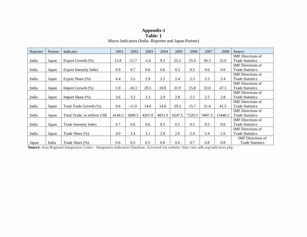
synergy effect than by simply adding up the strength of each country. The third is the stabilization of the regional economy. Based on the lessons from the Asian currency crisis, there have also been initiatives to strengthen linkages of policy-making in the region in order to create a regional economic structure that is resilient to global economic changes. In recent years, there have been active efforts by both India and Japan to conclude free trade agreement between them. Though Japan has been always a promoter of multilateral agreements, of late due to the emergence of different FTAs initiated by the United States, Japan has felt an acute need for its own treaty with different countries to protect its market share in world trade. India has always been a promoter of multilateral agreements, but emerging global trade environment has initiated India to enter into FTAs to increase its market share. Given India’s high tariff protection on a range of products, Japanese firms may gain significant market access from the proposed FTA. On the other hand, Indian suppliers can substantially increase their exports to the Japan given the proven capability of Indian firms and significant supply side capacity in India. However, the overall welfare gains for India will depend on the relative strength of the trade creation and trade diversion impacts. It is to be noted that India is the twelfth largest economy in the world by market exchange rates and the fourth largest by purchasing power parity (PPP) while the economy of the Japan is the second largest in the world by market exchange rates and third when adjusted for PPP. Both partners share a strong and rapidly growing trade and economic relationship. Further strengthening this relationship, the governments of Japan and India launched negotiations aimed at concluding a Comprehensive Economic Partnership Agreement (CEPA) in January 2007. The proposed CEPA should cover, but may not be limited to trade in goods, trade in services, measures for trade promotion, promotion, facilitation and liberalization of investment flows, measures for promoting economic cooperation in identified sectors and other areas for a comprehensive economic partnership between India and Japan. In this context, the main objectives of this paper are (i) to explore the feasibility of FTA between India and Japan, (ii) to simulate the gains and losses due to potential FTA between these countries and finally, (iv) what policy conclusions can be drawn as inputs into the policymaking process of FTA between India and Japan. The remainder paper is arranged as follows: Section 2 reviews bilateral trade relations between India and Japan. Section 3 research methodology and data bases. Section 4 presents various simulation scenarios. Section 5 reports and discusses the SMART and GTAP results. Section 6 discusses the systematic sensitivity analysis of GTAP results while Section 7 provides concluding remarks. 2. Bilateral Trade Relations between India and Japan India’s total trade with Japan has increased more than three times during 2001-08. It increased from US$ 4.1 billion in 2001 to US$ 13.4 billion in 2008. India’s exports to Japan have increased at the rate of 9.3% to 32% during 2001-08 while India’s imports from Japan have increased at the rate of 5.9% to 47% in the same period. However, the share of Japan in India’s exports has declined from 4% to 2.4% and imports have declined from 3.6% to 2.8% during 2001-08(See for details, table 1 in appendix-1). Despite increase in trade between India and Japan, it can be seen that the trade intensity for the India and Japan has been below optimum. The value of trade between two countries indicates that the extent of trade between the economies is low than would be expected on the basis of their importance in world trade. Table 1 in appendix-1 reveals that trade and export Intensity Index of India (TII) with Japan is less than 1 and remained so since 2001. Similarly, TII of Japan with India is also less than 1. TII indicates a bilateral trade flow is smaller than expected, given

3

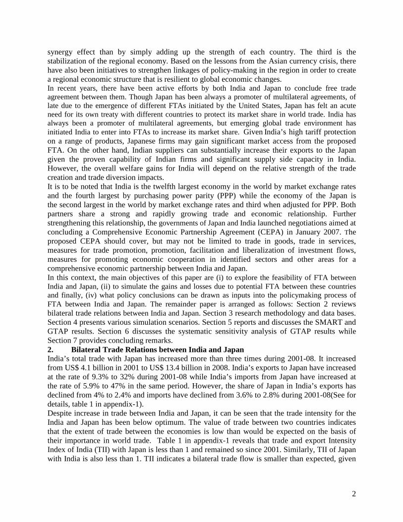
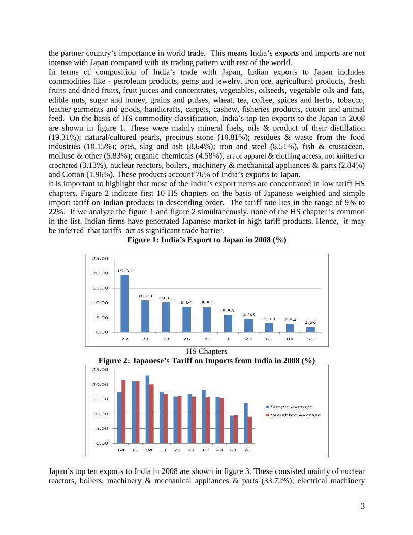
the partner country’s importance in world trade. This means India’s exports and imports are not intense with Japan compared with its trading pattern with rest of the world. In terms of composition of India’s trade with Japan, Indian exports to Japan includes commodities like - petroleum products, gems and jewelry, iron ore, agricultural products, fresh fruits and dried fruits, fruit juices and concentrates, vegetables, oilseeds, vegetable oils and fats, edible nuts, sugar and honey, grains and pulses, wheat, tea, coffee, spices and herbs, tobacco, leather garments and goods, handicrafts, carpets, cashew, fisheries products, cotton and animal feed. On the basis of HS commodity classification, India’s top ten exports to the Japan in 2008 are shown in figure 1. These were mainly mineral fuels, oils & product of their distillation (19.31%); natural/cultured pearls, precious stone (10.81%); residues & waste from the food industries (10.15%); ores, slag and ash (8.64%); iron and steel (8.51%), fish & crustacean, mollusc & other (5.83%); organic chemicals (4.58%), art of apparel & clothing access, not knitted or crocheted (3.13%), nuclear reactors, boilers, machinery & mechanical appliances & parts (2.84%) and Cotton (1.96%). These products account 76% of India’s exports to Japan. It is important to highlight that most of the India’s export items are concentrated in low tariff HS chapters. Figure 2 indicate first 10 HS chapters on the basis of Japanese weighted and simple import tariff on Indian products in descending order. The tariff rate lies in the range of 9% to 22%. If we analyze the figure 1 and figure 2 simultaneously, none of the HS chapter is common in the list. Indian firms have penetrated Japanese market in high tariff products. Hence, it may be inferred that tariffs act as significant trade barrier.

Figure 1: India’s Export to Japan in 2008 (%)

HS Chapters

Figure 2: Japanese’s Tariff on Imports from India in 2008 (%)

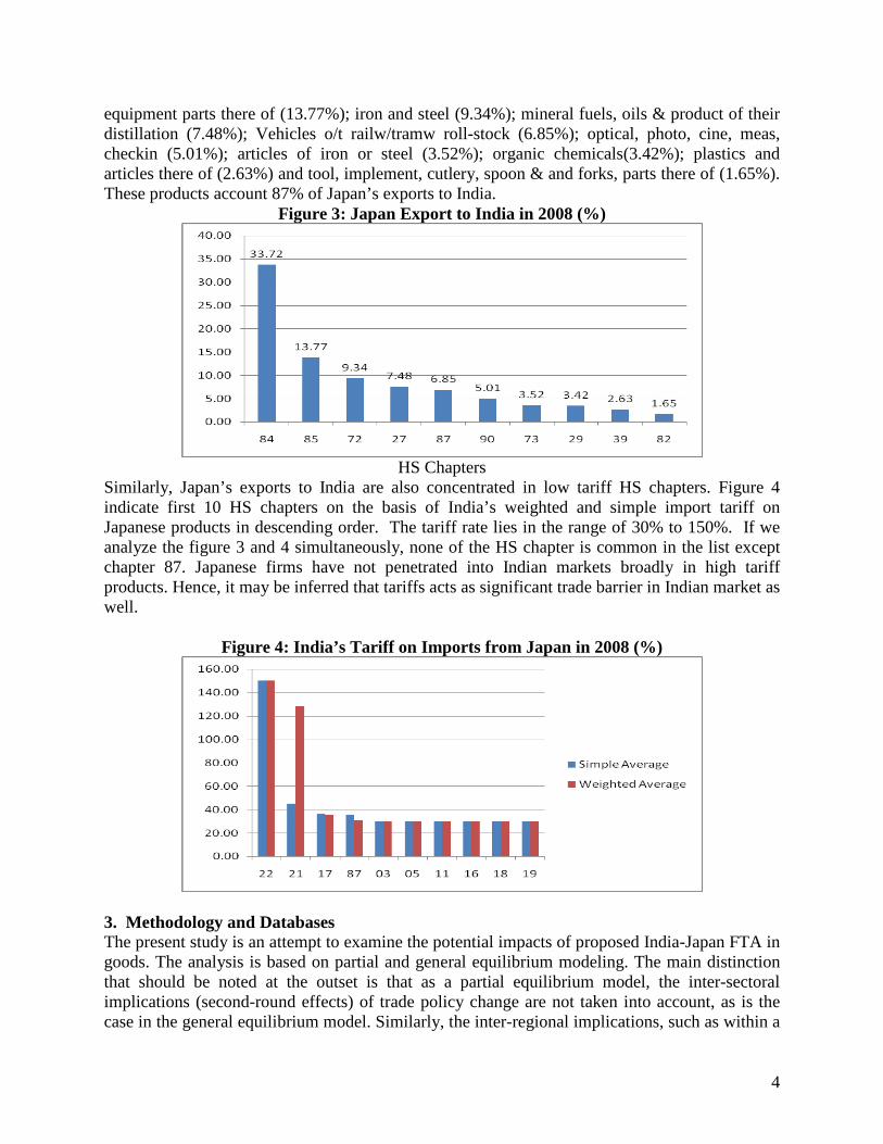
Japan’s top ten exports to India in 2008 are shown in figure 3. These consisted mainly of nuclear reactors, boilers, machinery & mechanical appliances & parts (33.72%); electrical machinery

4

equipment parts there of (13.77%); iron and steel (9.34%); mineral fuels, oils & product of their distillation (7.48%); Vehicles o/t railw/tramw roll-stock (6.85%); optical, photo, cine, meas, checkin (5.01%); articles of iron or steel (3.52%); organic chemicals(3.42%); plastics and articles there of (2.63%) and tool, implement, cutlery, spoon & and forks, parts there of (1.65%). These products account 87% of Japan’s exports to India.

Figure 3: Japan Export to India in 2008 (%)

HS Chapters

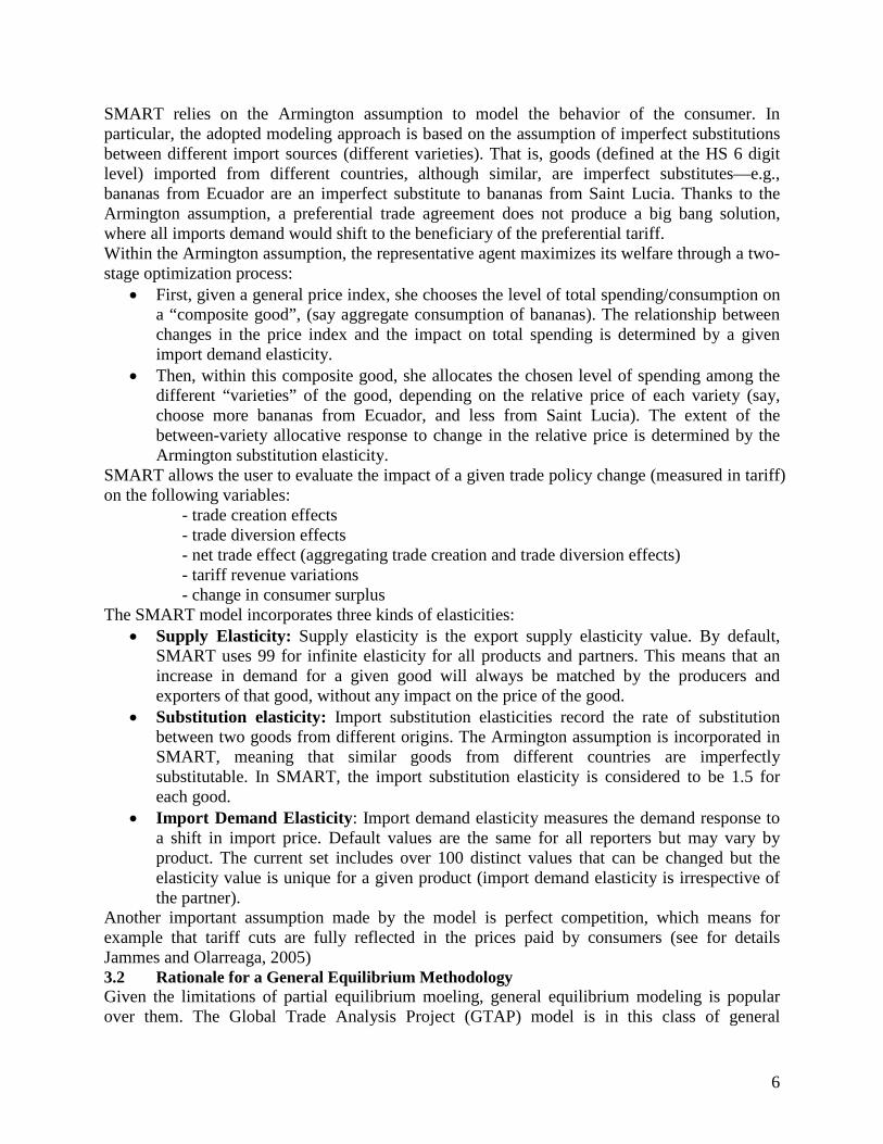
Similarly, Japan’s exports to India are also concentrated in low tariff HS chapters. Figure 4 indicate first 10 HS chapters on the basis of India’s weighted and simple import tariff on Japanese products in descending order. The tariff rate lies in the range of 30% to 150%. If we analyze the figure 3 and 4 simultaneously, none of the HS chapter is common in the list except chapter 87. Japanese firms have not penetrated into Indian markets broadly in high tariff products. Hence, it may be inferred that tariffs acts as significant trade barrier in Indian market as well.

Figure 4: India’s Tariff on Imports from Japan in 2008 (%)

3. Methodology and Databases The present study is an attempt to examine the potential impacts of proposed India-Japan FTA in goods. The analysis is based on partial and general equilibrium modeling. The main distinction that should be noted at the outset is that as a partial equilibrium model, the inter-sectoral implications (second-round effects) of trade policy change are not taken into account, as is the case in the general equilibrium model. Similarly, the inter-regional implications, such as within a

5

regional economic communities setting, are also ignored in a partial equilibrium framework. The only point of convergence between the partial and general equilibrium models is that it is still possible within a partial equilibrium model to analyze the trade policy effects on trade creation and diversion, welfare and tariff revenues while holding everything else constant. The general equilibrium models are popular over their partial equilibrium counterparts because they stress the interactions among different sectors. However, the partial equilibrium analysis models such as SMART can provide interesting information of the impact at a detailed product level. This section discusses in details the methodology applied for the empirical analysis. The discussion starts by outlining the SMART modeling and data framework. The SMART model analysis is further validated with a general equilibrium analysis model. The Global Trade Analysis Project (GTAP) model is used as a class of general equilibrium models. The GTAP methodology is therefore described in this section. 3.1 SMART-The Partial Equilibrium Modeling Framework 3.1.1 Rationale for Partial Equilibrium modeling SMART, the market access simulation package included in WITS, is a partial equilibrium modeling tool. While there are many different approaches to market access analysis, adopting the partial equilibrium one has a number of advantages. It also has a number of its disadvantages that the analyst ought to bear in mind. The main advantage of the partial equilibrium approach to Market Access Analysis is its minimal data requirement. In fact, the only required data for the trade flows, the trade policy (tariff), and a couple of behavioral parameters (elasticities). This can therefore take advantage of the rich WITS datasets which contain all of those. Another advantage (which follows directly from the minimal data requirement) is that it permits an analysis at a fairly disaggregated (or detailed) level. For example, it allows the study of the effects of the liberalization of “brown rice” imports by India, a level of aggregation that is neither convenient nor possible in the framework of a general equilibrium model. This also resolves a number of “aggregation biases.” The partial equilibrium approach also has a number of disadvantages that have to be kept in mind while conducting any analysis. Since it is only a “partial” model of the economy, the analysis is done on a pre-determined number of economic variables. This makes it very sensitive to a few (badly estimated) behavioral elasticities. Due to their simplicity also, partial equilibrium models may miss important interactions and feedbacks between various markets. In particular, the partial equilibrium approach tends to neglect the important inter-sectoral input/output (or upstream/downstream) linkages that are the basis of general equilibrium analyses. It also misses the existing constraints that apply to the various factors of production (e.g., labor, capital, land…) and their movement across sectors. 3.1.2 Theoretical Framework of SMART Model The setup of SMART is that, for a given good, different countries compete to supply (export to) a given home market. The focus of the simulation exercise is on the composition and volume of imports into that market. Export supply of a given good (say banana) by a given country supplier (say Ecuador) is assumed to be related to the price that it fetches in the export market. The degree of responsiveness of the supply of export to changes in the export price is given by the export supply elasticity. SMART assumes infinite export supply elasticity - that is, the export supply curves are flat and the world prices of each variety (e.g., bananas from Ecuador) are exogenously given. This is often called the price taker assumption. SMART can also operate with finite elasticity - upward sloping export supply functions – which entails a price effect in addition to the quantity effect.

6

SMART relies on the Armington assumption to model the behavior of the consumer. In particular, the adopted modeling approach is based on the assumption of imperfect substitutions between different import sources (different varieties). That is, goods (defined at the HS 6 digit level) imported from different countries, although similar, are imperfect substitutes—e.g., bananas from Ecuador are an imperfect substitute to bananas from Saint Lucia. Thanks to the Armington assumption, a preferential trade agreement does not produce a big bang solution, where all imports demand would shift to the beneficiary of the preferential tariff. Within the Armington assumption, the representative agent maximizes its welfare through a two-stage optimization process:

• First, given a general price index, she chooses the level of total spending/consumption on a “composite good”, (say aggregate consumption of bananas). The relationship between changes in the price index and the impact on total spending is determined by a given import demand elasticity.

• Then, within this composite good, she allocates the chosen level of spending among the different “varieties” of the good, depending on the relative price of each variety (say, choose more bananas from Ecuador, and less from Saint Lucia). The extent of the between-variety allocative response to change in the relative price is determined by the Armington substitution elasticity.

SMART allows the user to evaluate the impact of a given trade policy change (measured in tariff) on the following variables:

- trade creation effects - trade diversion effects - net trade effect (aggregating trade creation and trade diversion effects) - tariff revenue variations - change in consumer surplus

The SMART model incorporates three kinds of elasticities: • Supply Elasticity: Supply elasticity is the export supply elasticity value. By default,

SMART uses 99 for infinite elasticity for all products and partners. This means that an increase in demand for a given good will always be matched by the producers and exporters of that good, without any impact on the price of the good.

• Substitution elasticity: Import substitution elasticities record the rate of substitution between two goods from different origins. The Armington assumption is incorporated in SMART, meaning that similar goods from different countries are imperfectly substitutable. In SMART, the import substitution elasticity is considered to be 1.5 for each good.

• Import Demand Elasticity: Import demand elasticity measures the demand response to a shift in import price. Default values are the same for all reporters but may vary by product. The current set includes over 100 distinct values that can be changed but the elasticity value is unique for a given product (import demand elasticity is irrespective of the partner).

Another important assumption made by the model is perfect competition, which means for example that tariff cuts are fully reflected in the prices paid by consumers (see for details Jammes and Olarreaga, 2005) 3.2 Rationale for a General Equilibrium Methodology Given the limitations of partial equilibrium moeling, general equilibrium modeling is popular over them. The Global Trade Analysis Project (GTAP) model is in this class of general

7

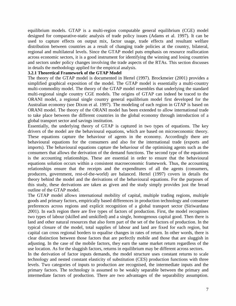
equilibrium models. GTAP is a multi-region computable general equilibrium (CGE) model designed for comparative-static analysis of trade policy issues (Adams et al. 1997). It can be used to capture effects on output mix, factor usage, trade effects and resultant welfare distribution between countries as a result of changing trade policies at the country, bilateral, regional and multilateral levels. Since the GTAP model puts emphasis on resource reallocation across economic sectors, it is a good instrument for identifying the winning and losing countries and sectors under policy changes involving the trade aspects of the RTAs. This section discusses in details the methodology applied for the empirical analysis. 3.2.1 Theoretical Framework of the GTAP Model The theory of the GTAP model is documented in Hertel (1997). Brockmeier (2001) provides a simplified graphical exposition of the model. The GTAP model is essentially a multi-country multi-commodity model. The theory of the GTAP model resembles that underlying the standard multi-regional single country CGE models. The origins of GTAP can indeed be traced to the ORANI model, a regional single country general equilibrium model first developed for the Australian economy (see Dixon et al. 1997). The modeling of each region in GTAP is based on ORANI model. The theory of the ORANI model has been extended to allow international trade to take place between the different countries in the global economy through introduction of a global transport sector and savings institution. Essentially, the underlying theory of GTAP is captured in two types of equations. The key drivers of the model are the behavioural equations, which are based on microeconomic theory. These equations capture the behaviour of agents in the economy. Accordingly there are behavioural equations for the consumers and also for the international trade (exports and imports). The behavioural equations capture the behaviour of the optimising agents such as the consumers that allows the derivation of the demand functions. The second type of the equations is the accounting relationships. These are essential in order to ensure that the behavioural equations solution occurs within a consistent macroeconomic framework. Thus, the accounting relationships ensure that the receipts and the expenditures of all the agents (consumers, producers, government, rest-of-the-world) are balanced. Hertel (1997) covers in details the theory behind the model and the derivations of the behavioural equations. For the purposes of this study, these derivations are taken as given and the study simply provides just the broad outline of the GTAP model. The GTAP model allows international mobility of capital, multiple trading regions, multiple goods and primary factors, empirically based differences in production technology and consumer preferences across regions and explicit recognition of a global transport sector (Siriwardana 2001). In each region there are five types of factors of production. First, the model recognises two types of labour (skilled and unskilled) and a single, homogenous capital good. Then there is land and other natural resources that also form part of the set of the factors of production. In the typical closure of the model, total supplies of labour and land are fixed for each region, but capital can cross regional borders to equalise changes in rates of return. In other words, there is clear distinction between those factors that are perfectly mobile and those that are sluggish in adjusting. In the case of the mobile factors, they earn the same market return regardless of the use location. As for the sluggish factors, returns in equilibrium may be different across sectors. In the derivation of factor inputs demands, the model structure uses constant returns to scale technology and nested constant elasticity of substitution (CES) production functions with three levels. Two categories of inputs to production are recognised, the intermediate inputs and the primary factors. The technology is assumed to be weakly separable between the primary and intermediate factors of production. There are two advantages of the separability assumption.

8

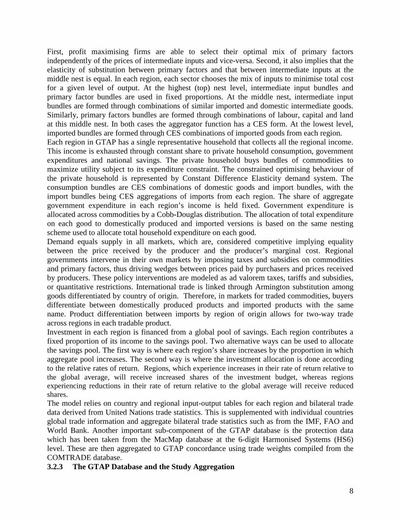
First, profit maximising firms are able to select their optimal mix of primary factors independently of the prices of intermediate inputs and vice-versa. Second, it also implies that the elasticity of substitution between primary factors and that between intermediate inputs at the middle nest is equal. In each region, each sector chooses the mix of inputs to minimise total cost for a given level of output. At the highest (top) nest level, intermediate input bundles and primary factor bundles are used in fixed proportions. At the middle nest, intermediate input bundles are formed through combinations of similar imported and domestic intermediate goods. Similarly, primary factors bundles are formed through combinations of labour, capital and land at this middle nest. In both cases the aggregator function has a CES form. At the lowest level, imported bundles are formed through CES combinations of imported goods from each region. Each region in GTAP has a single representative household that collects all the regional income. This income is exhausted through constant share to private household consumption, government expenditures and national savings. The private household buys bundles of commodities to maximize utility subject to its expenditure constraint. The constrained optimising behaviour of the private household is represented by Constant Difference Elasticity demand system. The consumption bundles are CES combinations of domestic goods and import bundles, with the import bundles being CES aggregations of imports from each region. The share of aggregate government expenditure in each region’s income is held fixed. Government expenditure is allocated across commodities by a Cobb-Douglas distribution. The allocation of total expenditure on each good to domestically produced and imported versions is based on the same nesting scheme used to allocate total household expenditure on each good. Demand equals supply in all markets, which are, considered competitive implying equality between the price received by the producer and the producer’s marginal cost. Regional governments intervene in their own markets by imposing taxes and subsidies on commodities and primary factors, thus driving wedges between prices paid by purchasers and prices received by producers. These policy interventions are modeled as ad valorem taxes, tariffs and subsidies, or quantitative restrictions. International trade is linked through Armington substitution among goods differentiated by country of origin. Therefore, in markets for traded commodities, buyers differentiate between domestically produced products and imported products with the same name. Product differentiation between imports by region of origin allows for two-way trade across regions in each tradable product. Investment in each region is financed from a global pool of savings. Each region contributes a fixed proportion of its income to the savings pool. Two alternative ways can be used to allocate the savings pool. The first way is where each region’s share increases by the proportion in which aggregate pool increases. The second way is where the investment allocation is done according to the relative rates of return. Regions, which experience increases in their rate of return relative to the global average, will receive increased shares of the investment budget, whereas regions experiencing reductions in their rate of return relative to the global average will receive reduced shares. The model relies on country and regional input-output tables for each region and bilateral trade data derived from United Nations trade statistics. This is supplemented with individual countries global trade information and aggregate bilateral trade statistics such as from the IMF, FAO and World Bank. Another important sub-component of the GTAP database is the protection data which has been taken from the MacMap database at the 6-digit Harmonised Systems (HS6) level. These are then aggregated to GTAP concordance using trade weights compiled from the COMTRADE database. 3.2.3 The GTAP Database and the Study Aggregation

9

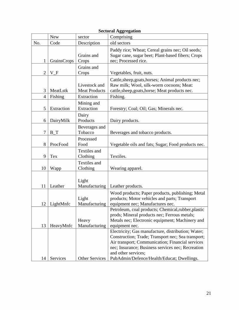
In the present study, GTAP database version 7, covering 113 countries/regions and 57 sectors, with a base year of 2004, have been used (Narayanan and Walmsley, 2008). All the trade flows for the 57 commodity categories are distinguished by their countries/regions of origin and destination, and on the basis of agents such as intermediate demand, final demand by private households, government and investment. The tariff data is mainly in the form of applied ad valorem rates. In the present analysis, 113 countries/regions are aggregated into 5 countries/regions and 57 commodities are aggregated into 14 commodity groups. Details of sectoral and regional aggregation are presented in Appendix-2. 4. Simulation Scenarios: 4.1 Partial Equilibrium Simulations

• Full trade liberalization between the two countries, this agreement being considered separately. All bilateral tariffs are completely and immediately eliminated.

4.2 General Equilibrium Simulations • Scenario-1 consider 100% tariff cut by India and Japan on imports from each other. In

this scenario, standard GTAP closures are adopted. • Scenario-2 consider 100% tariff cut by India and Japan on imports from each other. This

simulation is undertaken on the basis of modified standard closures for India. In India, there is typically an excess supply of unskilled labour, which can be drawn on by industries in the event of increased production. An assumption of full employment is inappropriate for countries like India. Hence, real wage rate has been fixed exogenously and the supply of labour is endogenised. This allowed us to take the effect on unemployment in India. However, full employment for Japan is assumed as per the standard assumption of GTAP. The outcomes of the simulations are reported in terms of its effect on prices, welfare, output, imports, exports and employment.

5. Simulation Results: 5.1 SMART Results In this section, the results of SMART model showing the possible impact of the FTA on India and Japan are discussed. One of the main justifications of liberalization is to reduce the price paid by consumers, increasing thus their purchasing power. So, our main objective is to analyze as accurately as possible consumers’ potential gain. Further, product-specific tariff revenues and trade effects has also been estimated. We choose to simulate the impact of a complete dismantlement of tariffs in order to clearly expose the effects of trade liberalization on all products. This is therefore an “extreme scenario” which aims at delineating the general trends of the impact of liberalization of both economies under the FTA. The results on trade creation and diversion are also reported. SMART simulation results reveal positive consumer’s surplus and trade creation effect for both India and Japan. The results are reported in table 1. As result of prospective India-Japan FTA, India’s consumer’s surplus will be increasing by US$ 737.9 million. India’s total trade creation effect is expected to be US$ 2763.8 million. Maximum trade creation effect for India is expected to be in HS chapter 87, chapter 84, chapter 27, chapter 35, chapter 72 and chapter 55 in descending order. It is to be noted that the most of the trade diversion is also expected in chapter 87, 84 and 48. There is little danger of import surges in products in chapter 22, 21, 17, 03, 05, 11, 16, 18 and 19 in which India has high tariff rate. Access may be granted in these tariff lines unless there are other concerns such as revenue loss or diverting cheaper products from other preferential arrangements.

10

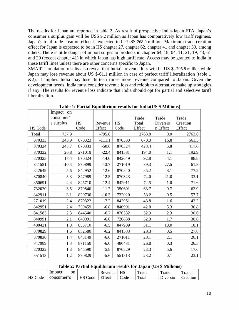
The results for Japan are reported in table 2. As result of prospective India-Japan FTA, Japan’s consumer’s surplus gain will be US$ 9.2 million as Japan has comparatively low tariff regimes. Japan’s total trade creation effect is expected to be US$ 268.0 million. Maximum trade creation effect for Japan is expected to be in HS chapter 27, chapter 62, chapter 41 and chapter 30, among others. There is little danger of import surges in products in chapter 64, 18, 04, 11, 21, 19, 43, 61 and 20 (except chapter 41) in which Japan has high tariff rate. Access may be granted to India in these tariff lines unless there are other concerns specific to Japan. SMART simulation results also reveal that India’s revenue loss will be US $ -795.8 million while Japan may lose revenue about US $-61.1 million in case of perfect tariff liberalization (table 1 &2). It implies India may lose thirteen times more revenue compared to Japan. Given the development needs, India must consider revenue loss and relook to alternative make up strategies, if any. The results for revenue loss indicate that India should opt for partial and selective tariff liberalization.

Table 1: Partial Equilibrium results for India(US $ Millions)

HS Code

Impact on consumer’s surplus

HS Code

Revenue Effect

HS Code

Trade Total Effect

Trade Diversion Effect

Trade Creation Effect

Total 737.9 -795.8 2763.8 0.0 2763.8 870333 343.9 870323 -111.1 870333 678.3 16.8 661.5 870324 243.7 870333 -50.6 870324 423.4 5.8 417.6 870332 26.8 271019 -22.4 841581 194.0 1.1 192.9 870323 17.4 870324 -14.0 842649 92.8 4.1 88.8 841581 10.4 870899 -13.7 271019 89.3 27.5 61.8 842649 5.6 842952 -12.6 870840 85.2 8.1 77.2 870840 5.3 847989 -12.5 870323 74.0 41.0 33.1 350691 4.4 845710 -12.4 842911 72.5 1.0 71.6 732020 3.5 870840 -11.7 350691 63.7 0.7 62.9 842911 3.1 820730 -10.3 732020 58.2 0.5 57.7 271019 2.4 870322 -7.2 842951 43.8 1.6 42.2 842951 2.4 730459 -6.8 840991 42.0 5.3 36.8 841583 2.3 844540 -6.7 870332 32.9 2.3 30.6 840991 2.1 840991 -6.6 720838 32.3 1.7 30.6 480431 1.8 853710 -6.5 847989 31.1 13.0 18.1 870829 1.6 852580 -6.2 841583 28.3 0.5 27.8 870830 1.4 843149 -6.0 271011 28.1 2.1 26.1 847989 1.3 871150 -6.0 480431 26.8 0.3 26.5 870322 1.3 845590 -5.8 870829 23.3 5.6 17.6 551513 1.2 870829 -5.6 551513 23.2 0.1 23.1

Table 2: Partial Equilibrium results for Japan (US $ Millions)

HS Code Impact on consumer’s HS Code

Revenue Effect

HS Code

Trade Total

Trade Diversio

Trade Creation

11

surplus

Effect n Effect Effect

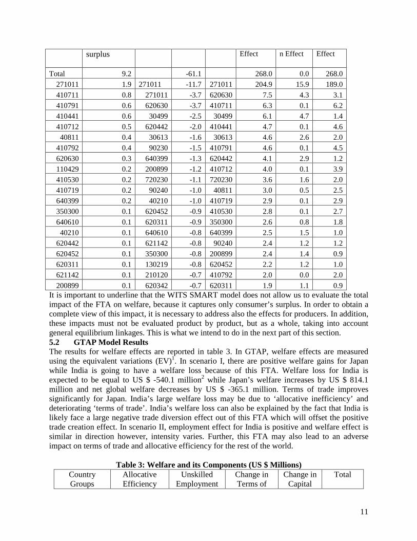
Total 9.2

-61.1 268.0 0.0 268.0 271011 1.9 271011 -11.7 271011 204.9 15.9 189.0 410711 0.8 271011 -3.7 620630 7.5 4.3 3.1 410791 0.6 620630 -3.7 410711 6.3 0.1 6.2 410441 0.6 30499 -2.5 30499 6.1 4.7 1.4 410712 0.5 620442 -2.0 410441 4.7 0.1 4.6 40811 0.4 30613 -1.6 30613 4.6 2.6 2.0

410792 0.4 90230 -1.5 410791 4.6 0.1 4.5 620630 0.3 640399 -1.3 620442 4.1 2.9 1.2 110429 0.2 200899 -1.2 410712 4.0 0.1 3.9 410530 0.2 720230 -1.1 720230 3.6 1.6 2.0 410719 0.2 90240 -1.0 40811 3.0 0.5 2.5 640399 0.2 40210 -1.0 410719 2.9 0.1 2.9 350300 0.1 620452 -0.9 410530 2.8 0.1 2.7 640610 0.1 620311 -0.9 350300 2.6 0.8 1.8 40210 0.1 640610 -0.8 640399 2.5 1.5 1.0

620442 0.1 621142 -0.8 90240 2.4 1.2 1.2 620452 0.1 350300 -0.8 200899 2.4 1.4 0.9 620311 0.1 130219 -0.8 620452 2.2 1.2 1.0 621142 0.1 210120 -0.7 410792 2.0 0.0 2.0 200899 0.1 620342 -0.7 620311 1.9 1.1 0.9

It is important to underline that the WITS SMART model does not allow us to evaluate the total impact of the FTA on welfare, because it captures only consumer’s surplus. In order to obtain a complete view of this impact, it is necessary to address also the effects for producers. In addition, these impacts must not be evaluated product by product, but as a whole, taking into account general equilibrium linkages. This is what we intend to do in the next part of this section. 5.2 GTAP Model Results The results for welfare effects are reported in table 3. In GTAP, welfare effects are measured using the equivalent variations (EV)1. In scenario I, there are positive welfare gains for Japan while India is going to have a welfare loss because of this FTA. Welfare loss for India is expected to be equal to US $ -540.1 million2

while Japan’s welfare increases by US $ 814.1 million and net global welfare decreases by US $ -365.1 million. Terms of trade improves significantly for Japan. India’s large welfare loss may be due to ‘allocative inefficiency’ and deteriorating ‘terms of trade’. India’s welfare loss can also be explained by the fact that India is likely face a large negative trade diversion effect out of this FTA which will offset the positive trade creation effect. In scenario II, employment effect for India is positive and welfare effect is similar in direction however, intensity varies. Further, this FTA may also lead to an adverse impact on terms of trade and allocative efficiency for the rest of the world.

Table 3: Welfare and its Components (US $ Millions) Country Groups

Allocative Efficiency

Unskilled Employment

Change in Terms of

Change in Capital

Total

12

effects

Effects

Trade

Stock

Scenario-I India -273.7 0 -194.8 -71.6 -540.1 Japan 74.6 0 859.1 -119.6 814.1

EU_27 -51.3 0 -64.5 48.6 -67.2 ODCs -43 0 -283.7 46.9 -279.8

Rest of World -71.5 0 -316.4 95.8 -292.1 Total -364.9 0 -0.2 0 -365.1

Scenario-II India -242 192.2 -200.2 -72.5 -322.6 Japan 74.6 0 858.3 -119.4 813.4

EU_27 -52.1 0 -65.7 48.8 -69 ODCs -42.9 0 -283.7 46.9 -279.8

Rest of World -72.4 0 -308.8 96.3 -284.9 Total -334.8 192.2 -0.2 0 -142.9

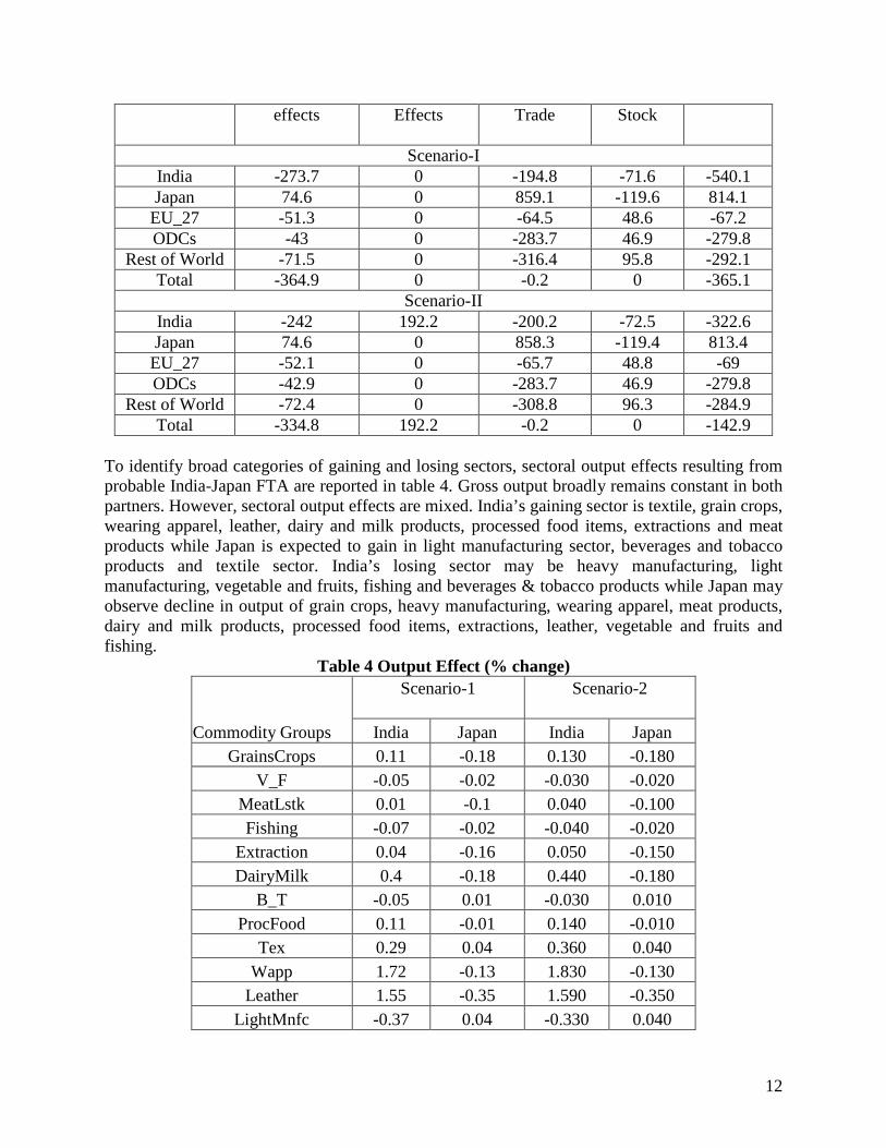
To identify broad categories of gaining and losing sectors, sectoral output effects resulting from probable India-Japan FTA are reported in table 4. Gross output broadly remains constant in both partners. However, sectoral output effects are mixed. India’s gaining sector is textile, grain crops, wearing apparel, leather, dairy and milk products, processed food items, extractions and meat products while Japan is expected to gain in light manufacturing sector, beverages and tobacco products and textile sector. India’s losing sector may be heavy manufacturing, light manufacturing, vegetable and fruits, fishing and beverages & tobacco products while Japan may observe decline in output of grain crops, heavy manufacturing, wearing apparel, meat products, dairy and milk products, processed food items, extractions, leather, vegetable and fruits and fishing.

Table 4 Output Effect (% change)

Commodity Groups

Scenario-1

Scenario-2

India Japan India Japan GrainsCrops 0.11 -0.18 0.130 -0.180

V_F -0.05 -0.02 -0.030 -0.020 MeatLstk 0.01 -0.1 0.040 -0.100 Fishing -0.07 -0.02 -0.040 -0.020

Extraction 0.04 -0.16 0.050 -0.150 DairyMilk 0.4 -0.18 0.440 -0.180

B_T -0.05 0.01 -0.030 0.010 ProcFood 0.11 -0.01 0.140 -0.010

Tex 0.29 0.04 0.360 0.040 Wapp 1.72 -0.13 1.830 -0.130

Leather 1.55 -0.35 1.590 -0.350 LightMnfc -0.37 0.04 -0.330 0.040

13

HeavyMnfc -0.28 -0.01 -0.250 -0.010 Services -0.01 0 0.030 0.000 CGDS 0.26 0.06 0.300 0.060 Total 0.00 0.00 0.032 0.006

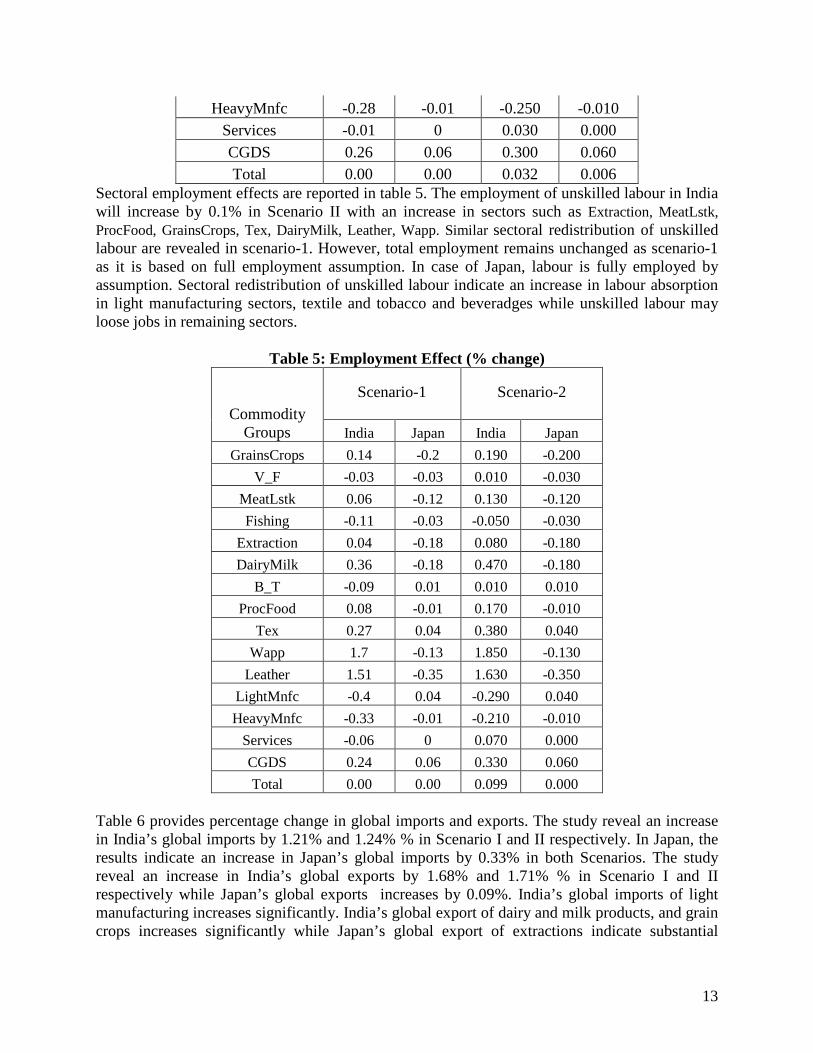
Sectoral employment effects are reported in table 5. The employment of unskilled labour in India will increase by 0.1% in Scenario II with an increase in sectors such as Extraction, MeatLstk, ProcFood, GrainsCrops, Tex, DairyMilk, Leather, Wapp. Similar sectoral redistribution of unskilled labour are revealed in scenario-1. However, total employment remains unchanged as scenario-1 as it is based on full employment assumption. In case of Japan, labour is fully employed by assumption. Sectoral redistribution of unskilled labour indicate an increase in labour absorption in light manufacturing sectors, textile and tobacco and beveradges while unskilled labour may loose jobs in remaining sectors.

Table 5: Employment Effect (% change)

Commodity

Groups

Scenario-1

Scenario-2

India Japan India Japan GrainsCrops 0.14 -0.2 0.190 -0.200

V_F -0.03 -0.03 0.010 -0.030 MeatLstk 0.06 -0.12 0.130 -0.120 Fishing -0.11 -0.03 -0.050 -0.030

Extraction 0.04 -0.18 0.080 -0.180 DairyMilk 0.36 -0.18 0.470 -0.180

B_T -0.09 0.01 0.010 0.010 ProcFood 0.08 -0.01 0.170 -0.010

Tex 0.27 0.04 0.380 0.040 Wapp 1.7 -0.13 1.850 -0.130

Leather 1.51 -0.35 1.630 -0.350 LightMnfc -0.4 0.04 -0.290 0.040 HeavyMnfc -0.33 -0.01 -0.210 -0.010

Services -0.06 0 0.070 0.000 CGDS 0.24 0.06 0.330 0.060 Total 0.00 0.00 0.099 0.000

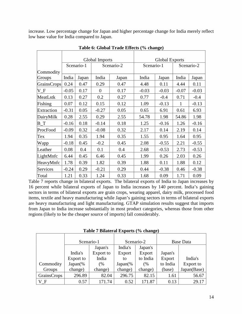
Table 6 provides percentage change in global imports and exports. The study reveal an increase in India’s global imports by 1.21% and 1.24% % in Scenario I and II respectively. In Japan, the results indicate an increase in Japan’s global imports by 0.33% in both Scenarios. The study reveal an increase in India’s global exports by 1.68% and 1.71% % in Scenario I and II respectively while Japan’s global exports increases by 0.09%. India’s global imports of light manufacturing increases significantly. India’s global export of dairy and milk products, and grain crops increases significantly while Japan’s global export of extractions indicate substantial

14

increase. Low percentage change for Japan and higher percentage change for India merely reflect low base value for India compared to Japan.

Table 6: Global Trade Effects (% change)

Commodity Groups

Global Imports Global Exports Scenario-1

Scenario-2

Scenario-1

Scenario-2

India Japan India Japan India Japan India Japan

GrainsCrops 0.24 0.47 0.29 0.47 4.48 0.11 4.44 0.11 V_F -0.05 0.17 0 0.17 -0.03 -0.03 -0.07 -0.03 MeatLstk 0.13 0.27 0.2 0.27 0.77 -0.4 0.71 -0.4 Fishing 0.07 0.12 0.15 0.12 1.09 -0.13 1 -0.13 Extraction -0.31 0.05 -0.27 0.05 0.65 6.91 0.61 6.93 DairyMilk 0.28 2.55 0.29 2.55 54.78 1.98 54.86 1.98 B_T -0.16 0.18 -0.14 0.18 1.25 -0.16 1.26 -0.16 ProcFood -0.09 0.32 -0.08 0.32 2.17 0.14 2.19 0.14 Tex 1.94 0.35 1.94 0.35 1.55 0.95 1.64 0.95 Wapp -0.18 0.45 -0.2 0.45 2.08 -0.55 2.21 -0.55 Leather 0.08 0.4 0.1 0.4 2.68 -0.53 2.73 -0.53 LightMnfc 6.44 0.45 6.46 0.45 1.99 0.26 2.03 0.26 HeavyMnfc 1.78 0.39 1.82 0.39 1.88 0.11 1.88 0.12 Services -0.24 0.29 -0.21 0.29 0.44 -0.38 0.46 -0.38 Total 1.21 0.33 1.24 0.33 1.68 0.09 1.71 0.09

Table 7 reports change in bilateral exports. The bilateral exports of India to Japan increases by 16 percent while bilateral exports of Japan to India increases by 140 percent. India’s gaining sectors in terms of bilateral exports are grain crops, wearing apparel, dairy milk, processed food items, textile and heavy manufacturing while Japan’s gaining sectors in terms of bilateral exports are heavy manufacturing and light manufacturing. GTAP simulation results suggest that imports from Japan to India increase substantially in most product categories, whereas those from other regions (likely to be the cheaper source of imports) fall considerably.

Table 7 Bilateral Exports (% change)

Commodity

Groups

Scenario-1 Scenario-2

Base Data

India's Export to Japan(% change)

Japan's Export to

India (%

change)

India's Export

to Japan(% change)

Japan's Export to India

(% change)

Japan's Export to India (base)

India's Export to

Japan(Base) GrainsCrops 296.89 82.04 296.75 82.15 1.61 56.67 V_F 0.57 171.74 0.52 171.87 0.13 29.17

15

MeatLstk 28.7 314.22 28.62 314.51 0.16 19.83 Fishing 12.17 41.6 12.07 41.71 0.51 2.99 Extraction 2.18 281.35 2.14 281.54 9.44 395.69 DairyMilk 3153.23 735.19 3154.63 735.29 0.08 2.27 B_T 99.68 163.46 99.70 163.51 0.48 1.11 ProcFood 16.03 452.27 16.05 452.37 2.49 441.79 Tex 30.03 189.71 30.15 189.71 67.49 207.94 Wapp 91.73 176.22 91.98 176.17 0.81 83.19 Leather 118.15 184.01 118.25 184.06 0.64 36.83 LightMnfc 2.85 196.19 2.89 196.24 858.13 747.03 HeavyMnfc 8.01 148.85 8.02 148.94 2460.99 657.93 Services 0.77 -0.79 0.79 -0.76 513.08 913.44 Total 16.41 140.83 16.43 140.90 3916.04 3595.88

6. Systematic Sensitivity Analysis Results from simulation models are sometimes highly dependent on parameter values such as substitution elasticities. In GTAP, the values of key economic parameters in the disaggregated database are derived from a survey of econometric work. Such estimates are most appropriately viewed as random. To address this issues, we conduct formal systematic sensitivity analysis3 (SSA) using the multivariate order three Gaussian Quadrature (GQ) procedure4

The results are reported in table 8. The SSA results for (+/-) 50 % shock around the default value of ESUBD indicate that welfare gains for Japan will remain positive in prospective India-Japan FTA and lies within 95 % confidence interval. The SSA results for India indicate both possibilities, negative and positive, with greater chance of having negative welfare gains. The SSA result for (+/- 50 %) shock around the default value of ESUBVA indicates positive welfare gains for Japan and lies within 95 % confidence interval and reverse are true for India. Thus, the SSA results for welfare gains remain positive for Japan and welfare loss for India irrespective of parameter values.

(Arndt, 1996; DeVusyst and Preckel, 1996). This analysis is an attempt to show how uncertain we are about modeling results given that there is some uncertainty over model inputs. It is a way of testing the robustness of the model results to these inputs.

Table 8: Systematic Sensitivity Analysis (Welfare Changes (US$ millions) Country Groups ESUBD (+/- 50% shock) ESUBVA (+/- 50% shock)

Default Mean SD 95 % C.I. Default Mean SD 95 % C.I.

India -540.08 -550.45 136.23 -1163.49 62.585 -540.08 -540.19 1.18 -545.5 -534.88 Japan 810.58 824.09 63.63 537.755 1110.425 810.58 810.65 0.84 806.87 814.43

EU_27 -67.45 -68.43 11.29 -119.235 -17.625 -67.45 -67.08 1.64 -74.46 -59.7 ODCs -279.78 -284.88 15.11 -352.875 -216.885 -279.78 -279.58 1.16 -284.8 -274.36 Rest of World -292.11 -296.53 16.74 -371.86 -221.2 -292.11 -292.54 2.79

-305.095 -279.985

ESUBD (+/- 50% shock) ESUBVA (+/- 50% shock)

16

Scenario-2 Scenario-2 EV Default Mean SD 95 % C.I. Default Mean SD 95 % C.I.

India -321.65 -332.55 134.35 -937.125 272.025 -321.65 -323.83 22.7 -425.98 -221.68 Japan 809.87 823.38 63.71 536.685 1110.075 809.87 809.89 0.8 806.29 813.49

EU_27 -69.19 -70.16 11.59 -122.315 -18.005 -69.19 -68.99 1.02 -73.58 -64.4 ODCs -279.8 -284.89 15.09 -352.795 -216.985 -279.8 -279.74 0.66 -282.71 -276.77 Rest of World -284.9 -289.39 17.41 -367.735 -211.045 -284.9 -285.21 1.74 -293.04 -277.38

7. Concluding Remarks The present study reveals that India and Japan’s consumer’s surplus will be increasing as result of this FTA. India’s gains are concentrated in few tariff lines in HS chapter 87, chapter 84, chapter 27, chapter 35, chapter 72 and chapter 55. This study also highlights the possibility of the trade diversion in chapter 87, 84 and 48. Access may be granted to Japan in products in chapter 22, 21, 17, 03, 05, 11, 16, 18 and 19 unless there are other concerns. In Japan, maximum trade creation effect is expected to be in HS chapter 27, chapter 62, chapter 41 and chapter 30, among others. Access may be granted to India in products in chapter 64, 18, 04, 11, 21, 19, 43, 61 and 20 unless there are other concerns. This study also shows that India may lose thirteen times more revenue compared to Japan. Given the development needs, India must consider revenue loss and relook to alternative make up strategies, if any. The results for revenue loss indicate that India should opt for partial and selective tariff liberalization. Indian and Japanese consumers will derive gains from the FTA since they will have access to goods at lower prices. To this point, it is assumed that producers and exporters will pass the benefits of tariff reductions on to consumers. If the benefits of tariff dismantlement are not passed on to consumers but are captured by the exporter or the importer, it is possible that there will be no increase in consumer welfare. It is therefore crucial to ensure that consumer welfare is transmitted to consumers. To this end, it is necessary that the competition policy shield consumers against possible abuse of potential dominant positions or against collusion from large importers. Competition policy capacities and the judicial system supporting it should therefore be strengthened to ensure that the FTA delivers its potential benefits. Despite consumer surplus gains, the CGE analysis concludes that India-Japan FTA would result in welfare loss for India. However, there are positive welfare gains for Japan. Terms of trade improve significantly for Japan while deteriorates for India. India’s large welfare loss may also be due to ‘allocative inefficiency’. The SSA results for welfare indicate that welfare gains remain positive for Japan and welfare loss for India irrespective of parameter values. This study also indicates that there is possibility of increase in bilateral exports as result of this FTA. Output and employment effects are mixed in both countries. There is positive effect on the demand for unskilled labour for India. It should be noted that the Indian export gains may not be materialized, despite tariff removal, due to the presence of non-tariff barriers. The predicted results may also be underestimated as the present analysis is based on comparative static CGE framework rather than dynamic CGE. For long term gains, the FTA between India and Japan must be comprehensive, including issues to trade in goods and services, and investment as India has no advantage in goods trade in perfect tariff liberalization at least in the short run. We also note the dynamic nature of the global trading environment, with implementation of other preferential agreements likely to impact on the outcomes of India- Japan FTA in goods.

17

Hence, the future research may be to identify non-tariff barriers, combined effect of multiple RTAs, investment opportunities and service trade in both markets. References: Adams, P. D., Horridge, K. M., Parmenter, B. R. and Zhang, X. 1998. “Long Run Effect on China of APEC Trade Liberalisation”, Centre of Policy Studies and the Impact Project, General Paper No. G-130, Monash University, http://www.monash.edu.au/policy/ftp/workpapr/g-130.pdf

Ahmed, Shahid. 2009. “Free Trade among South, East and South-East Asian Countries: A Step towards Asian Integration.” Foreign Trade Review XLIV(2):

Arndt, C. 1996. “An introduction to systematic sensitivity analysis via gaussian quadrature”, Center for Global Trade Analysis, Purdue University, https://www.gtap.agecon.purdue.edu/resources/download/39.pdf

Barro, R., and Sala-I-Martin, X. 1995. Economic Growth. New York: McGraw-Hill

Bhagwati, Jagdish, and Arvind Panagariya. 1999. “Preferential Trading Areas and Multilateralism” in Trading Blocs, ed. Jagdish Bhagwati, Pravin Krishna and Arvind Panagariya, 33–100. MIT Press.

Brockmeier, M. 2001. “A Graphical Exposition of the GTAP Model.” GTAP Technical Paper No. 8, Revised March 2001.

DeVuyst, E. A., and Preckel P. V. (1997) ‘Sensitivity analysis revisited: a quadrature-based approach’, Journal of Policy Modeling, Vol. 19, pp. 175-185.

Dixon, P.B., B.R. Parmenter, J. Sutton, and D.P. Vincent, ORANI: A Multisectoral Model of the Australian Economy, North-Holland Publishing Company.

Elizondom, R.L., and Krugman, P. 1992. “Trade Policy and Third World Metropolis.” NBER Working paper No. 4238. Washington, DC: National Bureau of economic Research.

Estevaleordal, Antoni. 2006. “The Rise of Regionalism.” Paper presented in the Conference, “The New Regionalism: Progress, Setbacks and Challenges” held at the Inter-American Development Bank, Washington, DC, February 9-10, 2006.

Gawande, K., and P. Krishna. 2001. “The Political Economy of Trade Policy: Empirical Approaches.” Working papers, Economics Department. Providence, RI: Brown University.

Hertel, T. W. Ed. 1997. “Global Trade Analysis: Modeling and Applications”, Cambridge: Cambridge University Press.

Jammes, O. and M. Olarreaga 2005. “Explaining SMART and GSIM”, The World Bank, http://wits.worldbank.org/witsweb/download/docs/Explaining_SMART_and_GSIM.pdf

Kalirajan K. 2007. “Regional Cooperation and Bilateral Trade Flows: An Empirical Measurement of resistance.” The International Trade Journal, 21(2): 85-107.

Kalirajan, K. 1999. “Stochastic Varying Coefficients Gravity Model: An Application in Trade Analysis.” Journal of Applied Statistics, 26: 185–194.

Lawrence, Robert. 1996. Regionalism, Multilateralism, and Deeper Integration. Washington: Brookings Institution.

18

Narayanan, G. Badri and Terrie L. Walmsley, Eds. 2008. Global Trade, Assistance, and Production: The GTAP 7 Data Base, Center for Global Trade Analysis, Purdue University. Available online at: http://www.gtap.agecon.purdue.edu/databases/v7/v7_doco.asp

Rodrik, D. 1998. “Why Do More Open Countries Have Large Governments?” Journal of Political Economy, 106 (5): 758–879

Siriwardana, M. 2001. “Some Trade Liberalization Options for Sri Lanka.” East Asian Studies

Review, 25(4): 453-477.

Wacziarg, R. 1997. Trade, Competition and market Size. Cambridge, MA: Harvard University.

Wilson, J. S., Mann, C. L. and T. Otsuki. 2004. “The Potential Benefit of Trade Facilitation: A Global Perspective.” World Bank Policy Research Working Paper 3224, February. Washington, DC: The World Bank

Endnotes: • Author is thankful to UNCTAD, Geneva and Prof. K. J. Joseph, CDS, Trivandrum for data access. 1. The regional household’s equivalent variation, resulting from a shock, is equal to the difference between

the expenditure required to obtain the new level of utility at initial prices and the initial expenditure. Thus, the EV uses the current prices as the base and asks what income change at the current prices would be equivalent to the proposed change in terms of its impact on utility.

2. A result different from partial equilibrium results 3. Systematic Sensitivity Analysis is an emerging technique that can incorporate information on distributions,

as opposed to single point estimates, in computable general equilibrium models. Arndt (1996) developed the SSA technique from recent advances in the area of numerical integration and its application to economic problems. The procedure automates solving the model as many times as necessary, once the user has set up and started it running.

4. A quadrature rule is an approximation of the definite integral of a function, usually stated as a weighted sum of function values at specified points within the domain of integration.

Appendix-1 Table: 1

Macro Indicators (India -Reporter and Japan-Partner) Reporter Partner Indicator 2001 2002 2003 2004 2005 2006 2007 2008 Source

India Japan Export Growth (%) 13.8 -11.7 -1.6 9.3 25.2 15.6 30.3 32.0 IMF Directions of Trade Statistics

India Japan Export Intensity Index 0.9 0.7 0.6 0.6 0.5 0.5 0.6 0.6 IMF Directions of Trade Statistics

India Japan Export Share (%) 4.4 3.5 2.9 2.5 2.4 2.3 2.3 2.4 IMF Directions of Trade Statistics

India Japan Import Growth (%) 5.9 -10.3 28.5 18.8 31.9 15.8 32.0 47.3 IMF Directions of Trade Statistics

India Japan Import Share (%) 3.6 3.2 3.3 2.9 2.8 2.5 2.5 2.8 IMF Directions of Trade Statistics

India Japan Total Trade Growth (%) 9.6 -11.0 14.0 14.8 29.3 15.7 31.4 41.5 IMF Directions of Trade Statistics

India Japan Total Trade, in million US$ 4144.5 3689.5 4207.8 4831.9 6247.5 7229.3 9497.3 13440.2 IMF Directions of Trade Statistics

India Japan Trade Intensity Index 0.7 0.6 0.6 0.5 0.5 0.5 0.5 0.6 IMF Directions of Trade Statistics

India Japan Trade Share (%) 4.0 3.4 3.1 2.8 2.6 2.4 2.4 2.6 IMF Directions of Trade Statistics

Japan India Trade Share (%) 0.6 0.5 0.5 0.6 0.6 0.7 0.8 0.8 IMF Directions of

Trade Statistics Source: Asia Regional Integration Center - Integration Indicators Database, Accessed via website: http://aric.adb.org/indicators.php

Appendix-2 Regional Aggregation

New region Comprising

No. Code Description old regions 1 India India India. 2 Japan

Japan.

3 EU_27 European Union 27

Austria; Belgium; Cyprus; Czech Republic; Denmark; Estonia; Finland; France; Germany; Greece; Hungary; Ireland; Italy; Latvia; Lithuania; Luxembourg; Malta; Netherlands; Poland; Portugal; Slovakia; Slovenia; Spain; Sweden; United Kingdom; Bulgaria; Romania.

4 ODCs

Other Developed Countries

Australia; New Zealand; Hong Kong; Korea; Taiwan; Singapore; Canada; United States of America; Switzerland; Norway; Rest of EFTA.

5 RestofWorld Rest of World

Rest of Oceania; China; Rest of East Asia; Cambodia; Indonesia; Lao People's Democratic Republ; Myanmar; Malaysia; Philippines; Thailand; Viet Nam; Rest of Southeast Asia; Bangladesh; Pakistan; Sri Lanka; Rest of South Asia; Mexico; Rest of North America; Argentina; Bolivia; Brazil; Chile; Colombia; Ecuador; Paraguay; Peru; Uruguay; Venezuela; Rest of South America; Costa Rica; Guatemala; Nicaragua; Panama; Rest of Central America; Caribbean; Albania; Belarus; Croatia; Russian Federation; Ukraine; Rest of Eastern Europe; Rest of Europe; Kazakhstan; Kyrgyztan; Rest of Former Soviet Union; Armenia; Azerbaijan; Georgia; Iran Islamic Republic of; Turkey; Rest of Western Asia; Egypt; Morocco; Tunisia; Rest of North Africa; Nigeria; Senegal; Rest of Western Africa; Central Africa; South Central Africa; Ethiopia; Madagascar; Malawi; Mauritius; Mozambique; Tanzania; Uganda; Zambia; Zimbabwe; Rest of Eastern Africa; Botswana; South Africa; Rest of South African Customs .

21

Sectoral Aggregation

New sector Comprising

No. Code Description old sectors

1 GrainsCrops Grains and Crops

Paddy rice; Wheat; Cereal grains nec; Oil seeds; Sugar cane, sugar beet; Plant-based fibers; Crops nec; Processed rice.

2 V_F Grains and Crops Vegetables, fruit, nuts.

3 MeatLstk Livestock and Meat Products

Cattle,sheep,goats,horses; Animal products nec; Raw milk; Wool, silk-worm cocoons; Meat: cattle,sheep,goats,horse; Meat products nec.

4 Fishing Extraction Fishing.

5 Extraction Mining and Extraction Forestry; Coal; Oil; Gas; Minerals nec.

6 DairyMilk Dairy Products Dairy products.

7 B_T Beverages and Tobacco Beverages and tobacco products.

8 ProcFood Processed Food Vegetable oils and fats; Sugar; Food products nec.

9 Tex Textiles and Clothing Textiles.

10 Wapp Textiles and Clothing Wearing apparel.

11 Leather Light Manufacturing Leather products.

12 LightMnfc Light Manufacturing

Wood products; Paper products, publishing; Metal products; Motor vehicles and parts; Transport equipment nec; Manufactures nec.

13 HeavyMnfc Heavy Manufacturing

Petroleum, coal products; Chemical,rubber,plastic prods; Mineral products nec; Ferrous metals; Metals nec; Electronic equipment; Machinery and equipment nec.

14 Services Other Services

Electricity; Gas manufacture, distribution; Water; Construction; Trade; Transport nec; Sea transport; Air transport; Communication; Financial services nec; Insurance; Business services nec; Recreation and other services; PubAdmin/Defence/Health/Educat; Dwellings.