Embed Size (px)
Citation preview

The
Auroral Large Imaging System—Design, operation and scientific results
Urban Brandstrom
IRF Scientific Report 279, 2003

The Auroral Large Imaging System—Design, operation and scientific results
Akademisk avhandlingsom med vederborligt tillstand av rektorsambetet vid Umea uni-versitet for avlaggande av filosofie doktorsexamen i rymdfysikframlagges till offentligt forsvar i IRF:s aula, fredagen den 13juni 2003, kl.9’ (09.15.00). Disputationsakten kommer att aga rum paengelska.
av
Urban Brandstrom, Institutet for rymdfysik, Kiruna
Fakultetsopponent
Dr. Kirsti Kauristie, Meteorologiska institutet, Helsingfors, Finland.
Sammanfattning: Ett gemensamt skandinaviskt markbaserat nat av automatise-rade stationer for avbildande norrskensstudier foreslogs 1989 av Ake Steen. Systemetgavs namnet ALIS efter engelskans “Auroral Large Imaging System”. De huvudsakligavetenskapliga motiven for detta aterfanns inom norrskensfysiken, men mojligheten attanvanda ALIS for andra andamal som tex. studier av polara stratosfarsmoln, meteoreroch liknande fenomen insags tidigt.
Denna avhandling fokuserar pa konstruktion och drift av en svensk prototyp till ALISbestaende av sex obemannade fjarrstyrda stationer i norra Sverige som ar inplacerade iett rutnat med ungefar fem mils sida. Vidare ges en sammanfattning av de vetenskapligaresultaten.
Varje station ar utrustad med en kanslig, hogupplosande (1024× 1024 bildelement)icke-bildforstarkt avbildande monokromatisk CCD detektor. Ett filterhjul med plats forsex smalbandiga interferensfilter mojliggor avbildande spektroskopiska absolutmatningarav tex. norrskensemissioner. Stationernas inbordes avstand (ca. 50 km) och synfalt (ca.50–60) ar anpassade sa att synfalten overlappar varandra. Detta gor det mojligt attanvanda triangulering och tomografiska metoder for att ta fram hojdinformation for deobserverade fenomenen.
ALIS var troligen ett av de forsta instrumenten som utnyttjade icke-bildforstark-ta hogkvalitativa CCD detektorer for spektroskopiska avbildande flerstationsstudier avljussvaga fenomen som tex. norrskensemissioner. Darvid ar absolutkalibrering av de av-bildande instrumenten ett lika viktigt som svart problem.
Aven om ALIS huvudsakligen byggdes for norrskensstudier, sa kom, helt ovantat,merparten av de vetenskapliga resultaten fran ett annat naraliggande omrade, namligenradio-inducerade optiska emissioner. ALIS gjorde de forsta otvetydiga observationerna avdetta fenomen pa hog latitud samt den forsta inversionen (med tomografiliknande meto-der) av hojdprofiler fran dessa data. Ovriga vetenskapliga resultat inkluderar uppskatt-ningar av norrskenets elektronspektra med tomografiska metoder, resultat fran koordine-rade matningar med satelliter och radarsystem samt studier av polara stratosfarsmoln.En ALIS-detektor anvandes vidare i ett samarbetsprojekt som resulterade i de forstamarkbaserade norrskensbilderna tagna under dagtid. Nyligen gjorde ALIS observationerav ett meteorspar fran en Leonid dar en preliminar studie ger vissa belagg for att vattenobserverats i meteorsparet.
Nyckelord: Flerstationsmatningar, Norrsken, Polara stratosfarsmoln, Radio-indu-
cerade optiska emissioner, Rymdfysik, Spektroskopiskt avbildande matningar, Tomografi.
The Auroral Large Imaging System—Design, operation and scientific results
Abstract: The Auroral Large Imaging System (ALIS) was proposed in 1989by Ake Steen as a joint Scandinavian ground-based network of automated auroralimaging stations. The primary scientific objective was in the field of auroral phy-sics, but it was soon realised that ALIS could be used in other fields, for examplestudies of Polar Stratospheric Clouds (PSC), meteors and other atmospheric phe-nomena.
This report describes the design, operation and scientific results from a Swe-dish prototype of ALIS consisting of six unmanned remote-controlled stationslocated in a grid of about 50 km in northern Sweden. Each station is equippedwith a sensitive high-resolution (1024×1024 pixels) unintensified monochromaticCCD-imager. A six-position filter-wheel for narrow-band interference filters faci-litates absolute spectroscopic measurements of, for example, auroral and airglowemissions. Overlapping fields-of-view resulting from the station baseline of about50 km combined with the station field-of-view of 50 to 60 enable triangulationas well as tomographic methods to be employed for obtaining altitude informationof the observed phenomena.
ALIS was probably one of the first instruments to take advantage of unintensi-fied (i.e. no image-intensifier) scientific-grade CCDs as detectors for spectroscopicimaging studies with multiple stations of faint phenomena such as aurora, airglow,etc. This makes absolute calibration a task that is as important as it is difficult.
Although ALIS was primarily designed for auroral studies, the majority of thescientific results so far have, quite unexpectedly, been obtained from observationsof HF pump-enhanced airglow. ALIS made the first unambiguous observationof this phenomenon at high latitudes and the first tomography-like inversion ofheight profiles of the airglow regions. The scientific results so far include tomo-graphic estimates of the auroral electron spectra, coordinated observations withsatellite and radar, as well as studies of polar stratospheric clouds. An ALISimager also participated in a joint project that produced the first ground-baseddaytime auroral images. Recently ALIS made spectroscopic observations of aLeonid meteor trail and preliminary analysis indicates the possible detection ofwater in the Leonid.
Keywords: Aurora, Artificial Airglow, HF pump-enhanced airglow, Multi-station measurements, Polar Stratospheric clouds, Radio-Induced optical emis-sions, Space physics, Spectroscopic imaging observations, Tomography.
IRF Scientific Report 279Language: EnglishISSN: 0284-1703ISBN: 91-7305-405-4 pp. 184 pages
Kiruna, April 2003
Urban Brandstrom
The
Auroral Large Imaging System—Design, operation and scientific results
Urban BrandstromSwedish Institute of Space Physics
Kiruna
April, 2003


Soli Deo Gloria
“Har jag i min tid nagot godt kunnat utratta, gifwen derfore Gudi aran!Hwad jag af mensklig swaghet felat, forlaten mig for Christi skull.”
Ur konung Gustaf 1:s afskedstal till rikets stander d. 16 juni 1560

Cover illustrations:The large image is a portion of an all-sky colour image (see Section C.1) of an activeauroral arc near zenith acquired on 12 December 2001 at 22:17:00 UTC with 4 sintegration time. The five small pictures are all obtained with ALIS and show (fromleft to right):
1. White-light (i.e. no filter) image of a pulsating aurora from 11 April 1994 at22:35:40 UTC obtained with 50 ms integration time by the ALIS station inKiruna.
2. A polar stratospheric cloud (see also Figure 6.16 and Section 6.6.1) on 9 Janu-ary 1997 at 14:19:30 UTC imaged in white-light and with 100 ms integrationtime by the ALIS station in Kiruna.
3. Top: The first unambiguous observations of HF pump-enhanced airglow thatoccurred on 16 February 1999 (see Section 6.4). The images are portions ofALIS images obtained at 17:32:25 UTC in the O(1D) 6300 A emission-linewith 5 s integration time at the ALIS station in Kiruna (left) and in Silkki-muotka (right). Bottom: A double-arc system imaged in the O(1S) 5577 Aemission-line on 25 March 1998 at 19:54:00 UTC by the ALIS imager in Silk-kimuotka (integration time 100 ms). This image is part of a data-set used toestimate the auroral electron-spectra, see Section 6.5.1.
4. A Leonid meteor trail captured by the Kiruna ALIS station with a 4227 Afilter on 19 November 2002 at 03:48:00 UTC with 20 s integration time.
5. The same meteor trail, but imaged with an adjacent ALIS imager in Kirunawith a 5893 A filter and 10 s integration time (refer to Section 6.6.2 for furtherinformation).
c©Urban BrandstromDoktorsavhandling vid Institutet for rymdfysikDoctoral thesis at the Swedish Institute of Space PhysicsThe Auroral Large Imaging System —Design, operation and scientific results.Online version and errata at: http://www.irf.se/~urban/avh/Typeset by the author in LATEX.Kiruna, April 2003Rev. 2
IRF Scientific Report 279ISSN 0284-1703ISBN 91-7305-405-4 pp. 184 pagesPrinted at the Swedish Institute of Space PhysicsBox 812SE-981 28, Kiruna, SwedenApril 2003

Sammanfattning
Ett gemensamt skandinaviskt markbaserat nat av automatiserade stationer foravbildande norrskensstudier foreslogs 1989 av Ake Steen. Systemet gavs namnetALIS efter engelskans “Auroral Large Imaging System”. De huvudsakliga veten-skapliga motiven for detta aterfanns inom norrskensfysiken, men mojligheten attanvanda ALIS for andra andamal som tex. studier av polara stratosfarsmoln,meteorer och liknande fenomen insags tidigt.
Denna avhandling fokuserar pa konstruktion och drift av en svensk prototyptill ALIS bestaende av sex obemannade fjarrstyrda stationer i norra Sverige somar inplacerade i ett rutnat med ungefar fem mils sida. Vidare ges en sammanfatt-ning av de vetenskapliga resultaten.
Varje station ar utrustad med en kanslig, hogupplosande (1024 × 1024 bilde-lement) icke-bildforstarkt avbildande monokromatisk CCD detektor. Ett filter-hjul med plats for sex smalbandiga interferensfilter mojliggor avbildande spekt-roskopiska absolutmatningar av tex. norrskensemissioner. Stationernas inbordesavstand (ca. 50 km) och synfalt (ca. 50–60) ar anpassade sa att synfaltenoverlappar varandra. Detta gor det mojligt att anvanda triangulering och tomo-grafiska metoder for att ta fram hojdinformation for de observerade fenomenen.
ALIS var troligen ett av de forsta instrumenten som utnyttjade icke-bild-forstarkta hogkvalitativa CCD detektorer for spektroskopiska avbildande flersta-tionsstudier av ljussvaga fenomen som tex. norrskensemissioner. Darvid ar abso-lutkalibrering av de avbildande instrumenten ett lika viktigt som svart problem.
Aven om ALIS huvudsakligen byggdes for norrskensstudier, sa kom, heltovantat, merparten av de vetenskapliga resultaten fran ett annat naraliggandeomrade, namligen radio-inducerade optiska emissioner. ALIS gjorde de forsta ot-vetydiga observationerna av detta fenomen pa hog latitud samt den forsta inver-sionen (med tomografiliknande metoder) av hojdprofiler fran dessa data. Ovrigavetenskapliga resultat inkluderar uppskattningar av norrskenets elektronspektramed tomografiska metoder, resultat fran koordinerade matningar med satelli-ter och radarsystem samt studier av polara stratosfarsmoln. En ALIS-detektoranvandes vidare i ett samarbetsprojekt som resulterade i de forsta markbaseradenorrskensbilderna tagna under dagtid. Nyligen gjorde ALIS observationer av ettmeteorspar fran en Leonid dar en preliminar studie ger vissa belagg for att vattenobserverats i meteorsparet.
Nyckelord: Flerstationsmatningar, Norrsken, Polara stratosfarsmoln, Radio-inducerade optiska emissioner, Rymdfysik, Spektroskopiskt avbildande matningar,Tomografi.

Abstract
The Auroral Large Imaging System (ALIS) was proposed in 1989 by Ake Steenas a joint Scandinavian ground-based network of automated auroral imaging sta-tions. The primary scientific objective was in the field of auroral physics, but itwas soon realised that ALIS could be used in other fields, for example studies ofPolar Stratospheric Clouds (PSC), meteors and other atmospheric phenomena.
This report describes the design, operation and scientific results from a Swe-dish prototype of ALIS consisting of six unmanned remote-controlled stationslocated in a grid of about 50 km in northern Sweden. Each station is equippedwith a sensitive high-resolution (1024×1024 pixels) unintensified monochromaticCCD-imager. A six-position filter-wheel for narrow-band interference filters facil-itates absolute spectroscopic measurements of, for example, auroral and airglowemissions. Overlapping fields-of-view resulting from the station baseline of about50 km combined with the station field-of-view of 50 to 60 enable triangulationas well as tomographic methods to be employed for obtaining altitude informationof the observed phenomena.
ALIS was probably one of the first instruments to take advantage of unintensi-fied (i.e. no image-intensifier) scientific-grade CCDs as detectors for spectroscopicimaging studies with multiple stations of faint phenomena such as aurora, air-glow, etc. This makes absolute calibration a task that is as important as it isdifficult.
Although ALIS was primarily designed for auroral studies, the majority of thescientific results so far have, quite unexpectedly, been obtained from observationsof HF pump-enhanced airglow. ALIS made the first unambiguous observationof this phenomenon at high latitudes and the first tomography-like inversionof height profiles of the airglow regions. The scientific results so far includetomographic estimates of the auroral electron spectra, coordinated observationswith satellite and radar, as well as studies of polar stratospheric clouds. An ALISimager also participated in a joint project that produced the first ground-baseddaytime auroral images. Recently ALIS made spectroscopic observations of aLeonid meteor trail and preliminary analysis indicates the possible detection ofwater in the Leonid.
Keywords: Aurora, Artificial Airglow, HF pump-enhanced airglow, Multi-station measurements, Polar Stratospheric clouds, Radio-Induced optical emis-sions, Space physics, Spectroscopic imaging observations, Tomography.

I
Preface
“Vi fa ej valja ramen for vart ode. Men vi ge den dess innehall. Den som villaventyret skall ocksa uppleva det — efter mattet av sitt mod. Den som villoffret skall offras — efter mattet av sin renhet.” Dag Hammarskjold
It is a great privilege to have the opportunity to finish this work that is an attempt toprovide a comprehensive compilation of material related to the Auroral Large ImagingSystem (ALIS). ALIS was conceived by Ake Steen, who had visions extending far beyondthis work, and nothing of what is reported here would have been made possible withouthis vision, enthusiasm, stubbornness and ability to acquire the necessary funding. Hisefforts, however, would have been impossible without the altruism and excellent lead-ership of Bengt Hultqvist, who was director of the Swedish Institute of Space Physics(IRF) 1957–1994. Bengt Hultqvist also read a draft of this work and provided muchvaluable advice. I also want to thank the present director of IRF, Rickard Lundin, aswell as Stanislav Barabash and Jan Pohjanen, for ensuring me the excellent undisturbedworking conditions that enabled me to complete this thesis. Thanks to Ingrid Sandahlfor taking care of ALIS since 2001.
To make a complete list of acknowledgements is virtually impossible, yet I feel obligedto attempt to list at least some names as representatives for a much larger group. I beginby specially thanking Lars Wittikko for many years of hard work in the ALIS project,and also as a representative of all those who deserved an acknowledgement, but havenever received one. My apologies for those painful, but equally unavoidable omissions! Ialso apologise now if I have, despite my best efforts, failed to provide proper referencesand credits anywhere.
A very special acknowledgement to Takehiko Aso and Masaki Ejiri, for their friend-ship, humble attitude, enthusiastic support of ALIS, inspiration and excellent ideas thatkept me from giving up many times. “Domo arrigato!”
I acknowledge Carl-Fredrik Enell, Bjorn Gustavsson, Peter Rydesater, Tima Sergi-enko and Asta Pellinen-Wannberg for their efforts with ALIS and ALIS data as well asfor countless hours of proofreading encouragement and much more. I am also very muchindebted to Carol Norberg and Rick McGregor who had the tedious task of correctingmy English and also provided many valuable comments. I thank Lars Nilsson as a per-sonification of those with the special gift of mastering the Art of computer programming.
I would also like to thank the past and present staff of IRF, ANS, EISCAT, ES-RANGE, NIPR, etc. represented by this far too short and incomplete list of names:Vesa Alatalo, Nils-Ake Andersson, Goran Axelsson, Peter Bergquist, Gote Johansson,Hugo Johansson, Jan Johansson, Magnus Johansson, Christer Juren, Juha Liikamaa,Aarne Luiro, Torbjorn Lovgren, Mats Luspa, Arne Mostrom, Olle Norberg, Jonas Olsen,Walter Puccio, Markus Rantakeisu, Akira Urashima, Bengt Wanhatalo and MasatoshiYamauchi. As representatives of the many co-authors and colleagues around the worldI would like to acknowledge Viktor Alpatov, Laila Andersson, Anasuya Aruliah, PaulBernhardt, Mikael Hedin, Ingemar Haggstrom, Jouni Jussila, Kari Kaila, Oleg Kornilov,Mike Kosch, Shu Lai, Hans Lauche, Thomas Leyser, William McNeil, Edmond Murad,
I

II
Michail Pudovkin, David Rees, Mike Rietveld, Tima Sergienko, Mikko Syrjasuo, TrondTrondsen, Bo Thide, Assar Westman, Ian McWhirter and Ola Widell.
Thanks to Trevor Preston, Maureen Ffitch and colleagues at AstroCam Ltd for valu-able discussions and help regarding the CCD camera and its software. A special acknow-ledgement goes to all the thousands of voluntary programmers making up the free andopen software communities. ALIS was funded through FRN (Forskningsradsnamnden),NFR (Naturvetenskapliga forskningsradet), Swedish National Space board (Rymdstyr-elsen, fjarranalyskommiten), IRF and Vetenskapsradet. Without the financial supportof the tax-payers of Sweden, Japan and other nations, as well as other funding sources,none of this research would have been possible.
I would have been completely unable to finish this work without the music of JohanSebastian Bach, Ludwig van Beethoven, Franz Berwald and many others. Dag Ham-marskjold’s book Vagmarken [Transl. as Markings; Hammarskjold , 1963, 1964] providedguidance and inspiration to carry on.
Ett alldeles speciellt tack till min mamma, Astrid Brandstrom, som stallt upp for migmer an nagon son kan begara. En stor kram till min fastmo Anette Snallfot, som talmodigthar statt ut med manga olagenheter pa grund av mina envisa forsok att fardigstalla dettaarbete. Tillraga pa allt drabbades hon av korrekturlasning och tryckeribestyr. Tack forallt stod och all uppmuntran, jag hade inte klarat mig utan er! Sist ett postumt tack tillalla de som pa manga satt bidragit till detta arbete men som aldrig fick uppleva dessfardigstallande.
Bjorkliden i april 2003
Urban Brandstrom
II
CONTENTS III
Contents
Preface I
1 Introduction 1
1.1 Auroral imaging . . . . . . . . . . . . . . . . . . . . . . . . . . . . 2
1.1.1 Auroral height estimations . . . . . . . . . . . . . . . . . . 3
1.1.2 Spectroscopic techniques . . . . . . . . . . . . . . . . . . . . 3
1.2 Summary . . . . . . . . . . . . . . . . . . . . . . . . . . . . . . . . 4
2 ALIS, the Auroral Large Imaging System. 5
2.1 The ALIS stations . . . . . . . . . . . . . . . . . . . . . . . . . . . 8
2.1.1 Scientific considerations . . . . . . . . . . . . . . . . . . . . 8
2.1.2 Selecting sites for the ALIS stations . . . . . . . . . . . . . 10
2.2 IT hardware and infrastructure . . . . . . . . . . . . . . . . . . . . 11
2.2.1 Computers . . . . . . . . . . . . . . . . . . . . . . . . . . . 13
2.2.2 The NIPU . . . . . . . . . . . . . . . . . . . . . . . . . . . . 13
2.2.3 Communication systems . . . . . . . . . . . . . . . . . . . . 15
2.2.4 Station data storage . . . . . . . . . . . . . . . . . . . . . . 16
2.2.5 Data archiving and availability . . . . . . . . . . . . . . . . 16
2.2.6 Operating Systems . . . . . . . . . . . . . . . . . . . . . . . 16
2.3 The ALIS control centre . . . . . . . . . . . . . . . . . . . . . . . . 17
3 The ALIS Imager 21
3.1 Some basic concepts . . . . . . . . . . . . . . . . . . . . . . . . . . 21
3.1.1 Spectral radiant sterance (radiance) . . . . . . . . . . . . . 21
3.1.2 The Rayleigh . . . . . . . . . . . . . . . . . . . . . . . . . . 22
3.1.3 Spectral radiant incidence (irradiance) . . . . . . . . . . . . 23
3.1.4 Number of incident photons . . . . . . . . . . . . . . . . . . 25
3.1.5 The CCD as a scientific imaging detector . . . . . . . . . . 25
3.1.6 Quantum efficiency . . . . . . . . . . . . . . . . . . . . . . . 25
3.1.7 Noise . . . . . . . . . . . . . . . . . . . . . . . . . . . . . . 26
3.1.8 Signal-to-noise ratio . . . . . . . . . . . . . . . . . . . . . . 27
3.1.9 The signal-to-noise ratio of an ICCD . . . . . . . . . . . . . 28
3.1.10 Threshold of detection and maximum signal . . . . . . . . . 29
3.1.11 Dynamic range . . . . . . . . . . . . . . . . . . . . . . . . . 30
3.2 Selecting an imager for ALIS . . . . . . . . . . . . . . . . . . . . . 30
3.2.1 Comparison of an ICCD with a CCD imager . . . . . . . . 30
3.2.2 Frame rate . . . . . . . . . . . . . . . . . . . . . . . . . . . 34
III
IV CONTENTS
3.3 The CCD imager for ALIS . . . . . . . . . . . . . . . . . . . . . . . 35
3.3.1 The camera head . . . . . . . . . . . . . . . . . . . . . . . . 353.3.2 The camera control unit . . . . . . . . . . . . . . . . . . . . 36
3.3.3 Configuring the imager . . . . . . . . . . . . . . . . . . . . 363.3.4 The user port . . . . . . . . . . . . . . . . . . . . . . . . . . 38
3.3.5 Operational remarks . . . . . . . . . . . . . . . . . . . . . . 383.4 The optical system . . . . . . . . . . . . . . . . . . . . . . . . . . . 39
3.5 Interference filters . . . . . . . . . . . . . . . . . . . . . . . . . . . 40
3.5.1 The filter wheel . . . . . . . . . . . . . . . . . . . . . . . . . 413.6 The camera positioning system . . . . . . . . . . . . . . . . . . . . 44
3.7 Summary . . . . . . . . . . . . . . . . . . . . . . . . . . . . . . . . 47
4 Calibrating ALIS 494.1 Removing the instrument signature . . . . . . . . . . . . . . . . . . 49
4.1.1 Bias removal . . . . . . . . . . . . . . . . . . . . . . . . . . 514.1.2 Dark-current . . . . . . . . . . . . . . . . . . . . . . . . . . 52
4.1.3 Flat-field correction . . . . . . . . . . . . . . . . . . . . . . 524.1.4 Bad-pixel correction . . . . . . . . . . . . . . . . . . . . . . 53
4.1.5 Summary . . . . . . . . . . . . . . . . . . . . . . . . . . . . 544.2 Intercalibration . . . . . . . . . . . . . . . . . . . . . . . . . . . . . 54
4.2.1 Absolute calibration . . . . . . . . . . . . . . . . . . . . . . 58
4.2.2 Removing the background . . . . . . . . . . . . . . . . . . . 614.2.3 Related issues . . . . . . . . . . . . . . . . . . . . . . . . . . 62
4.3 Geometrical calibration . . . . . . . . . . . . . . . . . . . . . . . . 62
5 Controlling ALIS 655.1 Making an observation with ALIS . . . . . . . . . . . . . . . . . . 66
5.1.1 Modes of operation . . . . . . . . . . . . . . . . . . . . . . . 685.1.2 Alarms and other exceptions . . . . . . . . . . . . . . . . . 68
5.2 OPERA . . . . . . . . . . . . . . . . . . . . . . . . . . . . . . . . . 695.2.1 User interfaces . . . . . . . . . . . . . . . . . . . . . . . . . 69
5.2.2 AIDA . . . . . . . . . . . . . . . . . . . . . . . . . . . . . . 69
5.2.3 Station software . . . . . . . . . . . . . . . . . . . . . . . . 715.2.4 Experiences and future plans . . . . . . . . . . . . . . . . . 72
6 Scientific results from ALIS 75
6.1 Scientific objectives of ALIS . . . . . . . . . . . . . . . . . . . . . . 766.2 ALIS data analysis . . . . . . . . . . . . . . . . . . . . . . . . . . . 78
6.2.1 Investigations of new data-analysis methods for ALIS . . . 786.3 Tomography and triangulation . . . . . . . . . . . . . . . . . . . . 83
6.3.1 Methods, initial studies and simulations . . . . . . . . . . . 836.3.2 Summary of results from computer tomography of ALIS-data 83
6.4 HF pump-enhanced airglow . . . . . . . . . . . . . . . . . . . . . . 85
6.4.1 The EISCAT Heating facility . . . . . . . . . . . . . . . . . 866.4.2 ALIS observations of enhanced airglow . . . . . . . . . . . . 86
6.4.3 Observations on 16 February 1999 . . . . . . . . . . . . . . 866.4.4 Discussion . . . . . . . . . . . . . . . . . . . . . . . . . . . . 94
6.5 Auroral studies . . . . . . . . . . . . . . . . . . . . . . . . . . . . . 101
IV
CONTENTS V
6.5.1 An estimate of the auroral electron spectra . . . . . . . . . 1026.5.2 Coordinated observations with satellite and radar . . . . . . 1056.5.3 Auroral vorticity . . . . . . . . . . . . . . . . . . . . . . . . 1056.5.4 Studies of the ionospheric trough . . . . . . . . . . . . . . . 1076.5.5 Daytime auroral imaging . . . . . . . . . . . . . . . . . . . 1076.5.6 The relation between the thermospheric neutral wind and
auroral events . . . . . . . . . . . . . . . . . . . . . . . . . . 1086.6 Other studies . . . . . . . . . . . . . . . . . . . . . . . . . . . . . . 110
6.6.1 Polar stratospheric clouds . . . . . . . . . . . . . . . . . . . 1106.6.2 Astronomical applications — water in a Leonid? . . . . . . 113
7 Concluding remarks 119
A The Instrumentation Platform 121A.1 Station housing . . . . . . . . . . . . . . . . . . . . . . . . . . . . . 122A.2 Environmental subsystems . . . . . . . . . . . . . . . . . . . . . . . 127A.3 Power subsystems . . . . . . . . . . . . . . . . . . . . . . . . . . . 127A.4 Housekeeping Unit . . . . . . . . . . . . . . . . . . . . . . . . . . . 130A.5 Timing . . . . . . . . . . . . . . . . . . . . . . . . . . . . . . . . . . 131A.6 Communication . . . . . . . . . . . . . . . . . . . . . . . . . . . . . 132A.7 Station computer . . . . . . . . . . . . . . . . . . . . . . . . . . . . 132A.8 The mobile imaging platform . . . . . . . . . . . . . . . . . . . . . 132
B Data for the ALIS imagers 135
C Related work 139C.1 A new digital all-sky camera . . . . . . . . . . . . . . . . . . . . . 139C.2 Colour video recordings of aurora . . . . . . . . . . . . . . . . . . . 141
D Continued operations with ALIS 145D.1 Assessing the present status of ALIS . . . . . . . . . . . . . . . . . 145
D.1.1 The ALIS imagers . . . . . . . . . . . . . . . . . . . . . . . 147D.2 Summary . . . . . . . . . . . . . . . . . . . . . . . . . . . . . . . . 149
D.2.1 A longer perspective . . . . . . . . . . . . . . . . . . . . . . 150
Bibliography 153
Index of acronyms 171
Index of notation 173
Index 177
V

VI CONTENTS
VI

LIST OF FIGURES VII
List of Figures
2.1 First proposed layout of ALIS . . . . . . . . . . . . . . . . . . . . . 6
2.2 Proposed layout of Swe-ALIS . . . . . . . . . . . . . . . . . . . . . 72.3 Fields-of-view and station baseline . . . . . . . . . . . . . . . . . . 9
2.4 Map of the present ALIS . . . . . . . . . . . . . . . . . . . . . . . . 122.5 The NIPU . . . . . . . . . . . . . . . . . . . . . . . . . . . . . . . . 14
2.6 The ALIS Control Centre . . . . . . . . . . . . . . . . . . . . . . . 172.7 Block-diagram of the ALIS Control Centre . . . . . . . . . . . . . . 18
2.8 The ALIS Operations Centre . . . . . . . . . . . . . . . . . . . . . 19
3.1 Quantum efficiency vs. wavelength for the SI-003AB CCD . . . . . 26
3.2 SNR vs. column emission . . . . . . . . . . . . . . . . . . . . . . . 313.3 SNR vs. integration time . . . . . . . . . . . . . . . . . . . . . . . . 33
3.4 The effect of on-chip binning . . . . . . . . . . . . . . . . . . . . . 33
3.5 Dividing a full-frame CCD into sub-arrays. . . . . . . . . . . . . . 343.6 The six ALIS imagers . . . . . . . . . . . . . . . . . . . . . . . . . 35
3.7 Schematic diagram of the optical system . . . . . . . . . . . . . . . 393.8 The six-position filter wheel . . . . . . . . . . . . . . . . . . . . . . 41
3.9 Electronics for the filter wheel and CPS . . . . . . . . . . . . . . . 433.10 The Camera Positioning System . . . . . . . . . . . . . . . . . . . 45
3.11 ALIS preset camera positions projected to 110 km altitude . . . . 463.12 Block diagram of ALIS imager subsystems . . . . . . . . . . . . . . 48
4.1 Coordinates and notation for the CCD in the ALIS Imager . . . . 504.2 Calibration sources used for ALIS calibration . . . . . . . . . . . . 55
4.3 Column emission rates for the calibrators . . . . . . . . . . . . . . 574.4 Example filter transmittance curve . . . . . . . . . . . . . . . . . . 59
4.5 Typical ALIS background image . . . . . . . . . . . . . . . . . . . 64
5.1 Block diagram of OPERA . . . . . . . . . . . . . . . . . . . . . . . 70
5.2 Station software . . . . . . . . . . . . . . . . . . . . . . . . . . . . 72
6.1 An example of the difficulties of auroral image classification. . . . . 80
6.2 Geometry of the HF pump-enhanced airglow experiments . . . . . 876.3 Maximum and average column emission time series as seen from
four stations . . . . . . . . . . . . . . . . . . . . . . . . . . . . . . . 89
6.4 Sequence of airglow images from the Silkkimuotka ALIS station . . 906.5 A series of images of enhanced 6300 A airglow . . . . . . . . . . . 91
6.6 Results of triangulation of the maximum volume emission. . . . . . 92
VII
VIII LIST OF FIGURES
6.7 Triangulation of the displacement of the two peaks in Figure 6.4 . 936.8 Fabry-Perot interferometer measurements of the neutral wind at
240 km altitude. . . . . . . . . . . . . . . . . . . . . . . . . . . . . 946.9 EISCAT UHF radar measurements of electron density . . . . . . . 956.10 Volume rendering of the artificially-enhanced airglow region above
Tromsø . . . . . . . . . . . . . . . . . . . . . . . . . . . . . . . . . 986.11 Estimates of the O(1D) excitation rates . . . . . . . . . . . . . . . 1006.12 Estimated electron flux . . . . . . . . . . . . . . . . . . . . . . . . 1036.13 Estimated electron flux . . . . . . . . . . . . . . . . . . . . . . . . 1046.14 Auroral images from 16 February 1997 . . . . . . . . . . . . . . . 1066.15 Daytime auroral image . . . . . . . . . . . . . . . . . . . . . . . . . 1096.16 PSC images and altitude profiles . . . . . . . . . . . . . . . . . . . 1126.17 ALIS images of a meteor trail . . . . . . . . . . . . . . . . . . . . . 1156.18 Projected meteor altitude profile . . . . . . . . . . . . . . . . . . . 1166.19 Meteoroid altitude profiles . . . . . . . . . . . . . . . . . . . . . . . 117
A.1 Block diagram of the GLIP . . . . . . . . . . . . . . . . . . . . . . 122A.2 Transmittance curves for plexi-glass . . . . . . . . . . . . . . . . . 124A.3 The GLIP in Tjautjas . . . . . . . . . . . . . . . . . . . . . . . . . 125A.4 Detail of the GLIP dome . . . . . . . . . . . . . . . . . . . . . . . . 126A.5 Electrical installation of a GLIP . . . . . . . . . . . . . . . . . . . 128A.6 Rear view of the Power Distribution Unit . . . . . . . . . . . . . . 129A.7 The Housekeeping Unit . . . . . . . . . . . . . . . . . . . . . . . . 130A.8 GPS-receiver . . . . . . . . . . . . . . . . . . . . . . . . . . . . . . 131A.9 The mobile imaging platform . . . . . . . . . . . . . . . . . . . . . 132
C.1 A digital colour all-sky camera . . . . . . . . . . . . . . . . . . . . 140C.2 Sample auroral image from the all-sky camera prototype . . . . . . 141C.3 Colour video frame of aurora with a meteor trail . . . . . . . . . . 143
D.1 Block diagram of the upgraded GLIP . . . . . . . . . . . . . . . . . 148D.2 Block diagram of future GLIPs . . . . . . . . . . . . . . . . . . . . 150D.3 A decentralised future ALIS . . . . . . . . . . . . . . . . . . . . . . 151
VIII
LIST OF TABLES IX
List of Tables
2.1 ALIS time-line . . . . . . . . . . . . . . . . . . . . . . . . . . . . . 62.2 Example imager coverages . . . . . . . . . . . . . . . . . . . . . . . 102.3 Geographical coordinates of the ALIS stations . . . . . . . . . . . . 11
3.1 ICCD parameters for the PAI . . . . . . . . . . . . . . . . . . . . . 313.2 Some CCD parameters for ccdcam5 . . . . . . . . . . . . . . . . . . 323.3 CCD-read noise at various pixel clocks . . . . . . . . . . . . . . . . 373.4 Filter placement standard for ALIS . . . . . . . . . . . . . . . . . . 423.5 Optional filters and their usage . . . . . . . . . . . . . . . . . . . . 423.6 ALIS preset camera positions . . . . . . . . . . . . . . . . . . . . . 47
4.1 Preset DC-bias levels . . . . . . . . . . . . . . . . . . . . . . . . . . 514.2 Total number of pixels and bias-pixels for the six ALIS imagers. . . 514.3 Results from recent intercalibration workshops . . . . . . . . . . . 564.4 Ratios of calibration results . . . . . . . . . . . . . . . . . . . . . . 574.5 Calibration results for ALIS . . . . . . . . . . . . . . . . . . . . . . 604.6 Measured fields-of-view for the ALIS imagers . . . . . . . . . . . . 63
6.1 Summary of image processing tools . . . . . . . . . . . . . . . . . . 786.2 Summary of data analysis tools . . . . . . . . . . . . . . . . . . . . 796.3 An auroral classification scheme . . . . . . . . . . . . . . . . . . . . 816.4 Overview of HF pump-enhanced airglow experiments with ALIS . 886.5 Filters for meteor studies . . . . . . . . . . . . . . . . . . . . . . . 114
A.1 GLIP Acronyms . . . . . . . . . . . . . . . . . . . . . . . . . . . . 123
B.1 Some CCD parameters for ccdcam1 . . . . . . . . . . . . . . . . . . 135B.2 Some CCD parameters for ccdcam2 . . . . . . . . . . . . . . . . . . 135B.3 Some CCD parameters for ccdcam3 . . . . . . . . . . . . . . . . . . 136B.4 Some CCD parameters for ccdcam4 . . . . . . . . . . . . . . . . . . 136B.5 Some CCD parameters for ccdcam5 . . . . . . . . . . . . . . . . . . 136B.6 Some CCD parameters for ccdcam6 . . . . . . . . . . . . . . . . . . 137
D.1 GLIP Acronyms . . . . . . . . . . . . . . . . . . . . . . . . . . . . 148
IX

X LIST OF TABLES
X
1
Chapter 1
Introduction
Stig min klang mot sol mot norrskensbagar vida,Vack sovande fjall, slumrande myr och mo!Vig at arbete in falt, som fruktsamma bida,Vig dem till sist en gang at den eviga tystnadens ro!
Albert Engstrom
“And I looked, and, behold, a whirlwind came out of the north, a greatcloud, and a fire infolding itself, and a brightness was about it, and outof the midst thereof as the colour of amber, out of the midst of the fire.”
Ezekiel 1:4
“Norr-skenets ratta hemvist, det hogsta av var atmospher, ar for oss och allavara undersokningar otilgangeligt. Ogat och synen aro de ende medel, hvilkatil rons inhamtande darvid kunna anvandas. Men afven dem ar ej tillatit, atskada Norr-skenen sadane som de aro i sig sjelfve, utan endast sa, som de,pa langt hall, visa sig for vara bedragliga omdomen.” Wilcke [1778]
The colourful and highly dynamic northern lights are one of the most fascinatingand beautiful phenomena seen in the night sky. For as long as there have beenpeople present at suitable locations, they have probably postulated over the originand purpose of the aurora, first in terms of myths, superstitious interpretations,or religious beliefs and later on in terms of scientific methods. Ancient works byAristotle [ca. 340 B.C.]; Pliny [ca. 77] and Seneca [ca. 63] with vivid descriptionsof low latitude aurora are reported by Chamberlain [1995]. It is sometimes spec-ulated if some ancient biblical texts might contain early descriptions of auroralevents, such as, for example the vision of Ezeikel around 593 B.C., as quotedabove [Siscoe et al., 2002; Raspopov et al., 2003, and references therein].
Many sources report that the name: “Aurora Borealis” (northern lights) wasassigned by Gassendi [1651], however, research by Siscoe [1978] indicates thatthese terms existed earlier, and that they might be traceable to Galileo Galileior his disciple Guiducci [Eather , 1980, p. 51].
When modern science emerged, explanations of the aurora began to be for-mulated. Initially only visual observations were available [for example Gassendi ,1651; Celsius, 1733; de Mairan, 1733]. In a speech to the king (Gustav III) and
1
2 CHAPTER 1. INTRODUCTION
the newly established Royal Swedish Academy of Sciences, Wilcke [1778] sum-marises “the newest explanations of the northern lights”. This speech includes alarge set of early references.∗ Wilcke also remarks on the exceptional difficultiesto make accurate recordings of auroral events. “The eye, the pen, and the brushof the fastest painter are too slow to record the changes”†. Yet, it would takemore than one century until better tools became available. Meanwhile, artisticwork, like drawings and paintings were the only available tools to record observa-tions of northern lights [see references in Eather , 1980; Pellinen and Kaila, 1991].Now, over 225 years later, and despite the giant leaps of technology, it is still arather difficult task to make accurate auroral recordings.
1.1 Auroral imaging
Following the invention of photography the first successful picture of the au-rora was taken by Brendel in 1892 [Baschin, 1900]. This paved the way formulti-station auroral imaging. One of the first large-scale auroral observationcampaigns involving several stations was carried out by Birkeland [1908, 1913].
The most well-known imaging instrument is maybe the All-Sky Camera(ASC), which consists of a camera together with an optical arrangement of oneor several mirrors providing near 180 field-of-view. This instrument exists ina variety of designs [for example Stoffregen, 1955, 1956; Elvey and Stoffregen,1957; Hypponen et al., 1974, and others] and was pioneered by Gartlein [1947].During the International Geophysical Year (IGY) of 1957–1958 a ground-basednetwork of all-sky cameras was operating at 114 stations around the polar regions[Stoffregen, 1962]. Since then, improved versions of the all-sky camera have beenthe main observatory instruments for ground-based imaging of the aurora. Ex-amples of present state-of-the-art digital all-sky cameras are the all-sky opticalimager (ASI) in use at the Amudsen-Scott South Pole station [Ejiri et al., 1998,1999] as well as the cameras used in the Finnish MIRACLE network‡ [Syrjasuo,1996; Syrjasuo, 1997; Syrjasuo, 2001]. These all-sky cameras represent a con-siderable improvement over earlier instruments. Since a filter-wheel is present,spectroscopic measurements are possible. A somewhat different, and less ad-vanced approach, is presented in Section C.1, where a commercial digital colourcamera is used.
The intense development of television cameras starting in the late 1940’s ledto the emergence of better low-light imaging detectors based on television image-tubes, for example image orthicons and intensified vidicons. This enabled directelectronic recording of auroral image data. Absolute measurements with thisclass of detectors is very difficult, mainly due to calibration difficulties related totheir non-linear response. Therefore these detectors have mainly been used forwhite-light imaging.
According to Jones [1974], the first use of image orthicon television cam-era systems for auroral observations were by Davis and Hicks [1964]. Image-intensified vidicon tubes were introduced by Scourfield and Parsons [1969]. Since
∗See also [Chamberlain, 1995, Appendix VIII], regarding historical references.†Free translation by the author, see the quote at the beginning of Chapter 3‡http://www.geo.fmi.fi/MIRACLE/
2
1.1. AURORAL IMAGING 3
then, technology has improved considerably and there exists a plethora of au-roral imagers based on television type cameras, often in a combination with animage intensifier. An example of a modern television-type imager is the excel-lent Portable Auroral Imager (PAI) intended for high-resolution auroral imaging[Trondsen, 1998]. A few more examples of television-type imagers are mentionedin Section 3.2.1.
Space-borne optical imagers simplified the monitoring of large-scale auroralfeatures. The Viking imager [Anger et al., 1987] may serve as an excellent exampleof this [see Pellinen and Kaila, 1991, for a more complete listing of space-borneimagers]. Polar/VIS§ is a more recent example of the versatile capabilities ofspace-borne auroral imaging techniques. For global auroral imaging, the capab-ility to use UV-emissions to measure sunlit day-side aurora is a great advantage[Steen, 1989]. However, auroral imaging from space does not make ground-basedand rocket-borne studies obsolete, they are both powerful and complementarymethods that should not be underestimated. For example, small- and medium-scale phenomena are difficult to study from space due to the spatial smearingcaused by the orbital motion, as well as imprecisely known value of the effectivealbedo [Steen, 1989]. Furthermore the orbital motion prohibits continuous stud-ies in a certain local time sector, as well as along a certain magnetic field-line.The best results tend to emerge when different observing methods are combined.
1.1.1 Auroral height estimations
The number of reliable height estimations of the aurora before those obtainedfrom photographic methods are very few [Størmer , 1955]. The first measurementof the height of an aurora was made between 1726 and 1730 by de Mairan [1733]resulting in an estimated height of about 400–1300 km. Further reading on earlyheight determinations is found in the works of Wilcke [1778]; Størmer [1955], andreferences therein.
By obtaining auroral photographs simultaneously from two or more locations,it is possible to employ triangulation techniques to estimate the height of theaurora. The first results from this method were obtained by Størmer [1911].Later on the methods were improved and simplified [for example Vegard andKrogness, 1920], as described in the cornerstone work by Størmer [1955].
For examples of more recent height-determinations of the aurora see Brandyand Hill [1964]; Romick and Belon [1967]; Brown et al. [1976]; Stenbaek-Nielsenand Hallinan [1979]; Kaila [1987]; Steen [1988a,b]; Aso et al. [1990]; Jones et al.[1991]; Aso et al. [1993, 1994]; Frey et al. [1996], and references therein. However,embarking onto a detailed discussion of the many recent measurements extendfar beyond the scope of this introduction.
1.1.2 Spectroscopic techniques
The auroral signal contains a considerable amount of spectral information. Thefirst measurements of the auroral spectra were carried out by Angstrom [1868,1869]. He also named the convenient unit Angstrom (1 A = 0.1 nm). Another
§http://eiger.physics.uiowa.edu/~vis/
3
4 CHAPTER 1. INTRODUCTION
important contributor to auroral spectroscopy was Vegard [1913]. Further in-formation on auroral spectra, as well as more references are provided by Jones[1974] and Chamberlain [1995].
Sadly, spectrographs and spectrometers are rare instruments in present dayauroral studies. As much more sensitive detectors exist today, a re-examinationof the spectral features of the aurora might prove rewarding.
At the present time, the dominating instrument for spectroscopic studies ofaurora is the interference filter photometer. This instrument is used either forfixed single-point measurements, or in a scanning or imaging configuration. Ex-amples of contemporary instruments are found in Kaila [2003a].
1.2 Summary
This short introduction can in no way provide a complete overview of the field.Hopefully, it has at least provided a set of references for further studies and arudimentary background to the desire to build ALIS as a multi-station imagingnetwork capable of absolute spectroscopic measurements of column emission rateswithin the field-of-view of a traditional all-sky camera, as well as the capabilityto image a common volume, thus enabling triangulation and auroral tomography.
For further reading related to low-light optical instrumentation for auroralmeasurements see, for example, Høymork [2000], and references therein. Galperin[2001] presents an interesting discussion regarding the multiple scales of auroralphenomena. Such considerations are important for selecting a suitable baselineand field-of-view of a multi-station imaging system. An extensive review of in-struments and networks for optical auroral studies was presented by Pellinen andKaila [1991]. This was about the same time as work on ALIS commenced andtherefore their work is recommended as an additional introduction, as well as anillustration of the power of coordinated studies with many instruments, regardlessof whether they are ground-based or space-borne.
This work is organised in seven chapters and four appendices. A readeronly interested in the scientific results from ALIS might wish to skip directlyto Chapter 6, however, please consider quickly browsing through Chapters 2–4for an introduction to the possibilities and limitations of the instrument. Tech-nical details, related work and future plans are deferred to the appendices.
4
5
Chapter 2
ALIS, the Auroral LargeImaging System.
“One of the symptoms of an approaching nervous breakdown is the beliefthat one’s work is terribly important.” Bertrand Russell
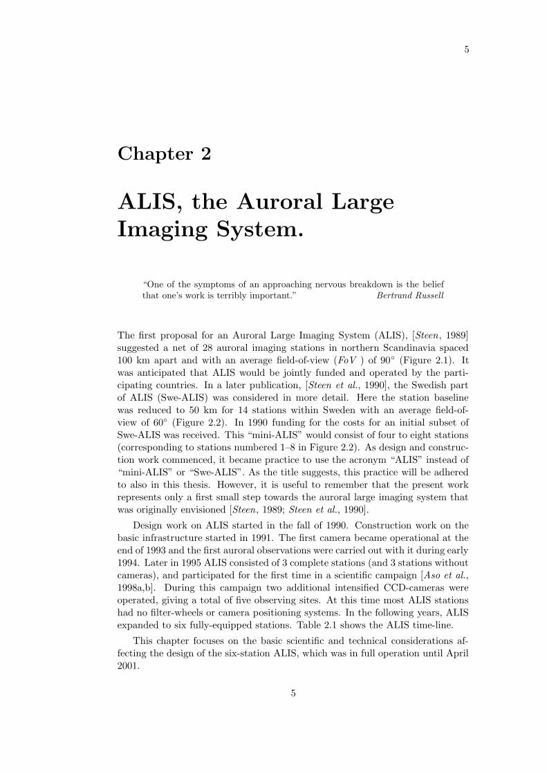
The first proposal for an Auroral Large Imaging System (ALIS), [Steen, 1989]suggested a net of 28 auroral imaging stations in northern Scandinavia spaced100 km apart and with an average field-of-view (FoV ) of 90 (Figure 2.1). Itwas anticipated that ALIS would be jointly funded and operated by the parti-cipating countries. In a later publication, [Steen et al., 1990], the Swedish partof ALIS (Swe-ALIS) was considered in more detail. Here the station baselinewas reduced to 50 km for 14 stations within Sweden with an average field-of-view of 60 (Figure 2.2). In 1990 funding for the costs for an initial subset ofSwe-ALIS was received. This “mini-ALIS” would consist of four to eight stations(corresponding to stations numbered 1–8 in Figure 2.2). As design and construc-tion work commenced, it became practice to use the acronym “ALIS” instead of“mini-ALIS” or “Swe-ALIS”. As the title suggests, this practice will be adheredto also in this thesis. However, it is useful to remember that the present workrepresents only a first small step towards the auroral large imaging system thatwas originally envisioned [Steen, 1989; Steen et al., 1990].
Design work on ALIS started in the fall of 1990. Construction work on thebasic infrastructure started in 1991. The first camera became operational at theend of 1993 and the first auroral observations were carried out with it during early1994. Later in 1995 ALIS consisted of 3 complete stations (and 3 stations withoutcameras), and participated for the first time in a scientific campaign [Aso et al.,1998a,b]. During this campaign two additional intensified CCD-cameras wereoperated, giving a total of five observing sites. At this time most ALIS stationshad no filter-wheels or camera positioning systems. In the following years, ALISexpanded to six fully-equipped stations. Table 2.1 shows the ALIS time-line.
This chapter focuses on the basic scientific and technical considerations af-fecting the design of the six-station ALIS, which was in full operation until April2001.
5
6 CHAPTER 2. ALIS, THE AURORAL LARGE IMAGING SYSTEM.
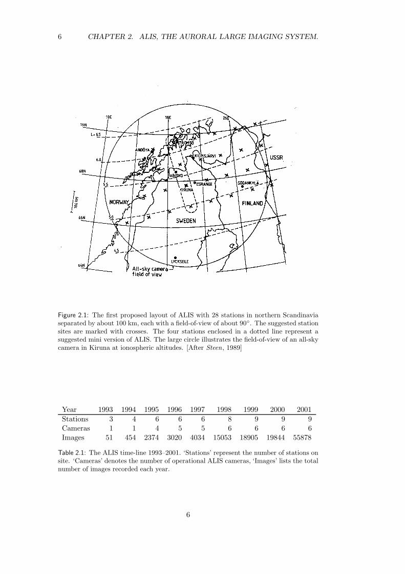
Figure 2.1: The first proposed layout of ALIS with 28 stations in northern Scandinaviaseparated by about 100 km, each with a field-of-view of about 90. The suggested stationsites are marked with crosses. The four stations enclosed in a dotted line represent asuggested mini version of ALIS. The large circle illustrates the field-of-view of an all-skycamera in Kiruna at ionospheric altitudes. [After Steen, 1989]
Year 1993 1994 1995 1996 1997 1998 1999 2000 2001
Stations 3 4 6 6 6 8 9 9 9Cameras 1 1 4 5 5 6 6 6 6Images 51 454 2374 3020 4034 15053 18905 19844 55878
Table 2.1: The ALIS time-line 1993–2001. ‘Stations’ represent the number of stations onsite. ‘Cameras’ denotes the number of operational ALIS cameras, ‘Images’ lists the totalnumber of images recorded each year.
6
7
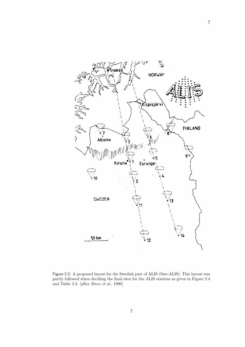
Figure 2.2: A proposed layout for the Swedish part of ALIS (Swe-ALIS). This layout waspartly followed when deciding the final sites for the ALIS stations as given in Figure 2.4and Table 2.3. [after Steen et al., 1990]
7

8 CHAPTER 2. ALIS, THE AURORAL LARGE IMAGING SYSTEM.
2.1 The ALIS stations
The design and deployment of the ALIS stations involves a large number ofconsiderations. Each station must be designed for unmanned remote-controlledoperation during extended time-periods in low-population regions with a sub-arctic climate. The technical design of the ALIS-station, which constitutes aGround-based Low-light Imaging Platform (GLIP), is considered in Appendix A.
The main scientific instrument at the ALIS-station is the ALIS-imager (cov-ered in detail in Chapter 3). Although the stations are primarily designed foroptical instrumentation, the design permits a variety of other instruments to sharethe common infrastructure. The general requirement on any additional scientificmodule is that it fits physically, does not interfere with existing equipment andis compatible with the resources available at the GLIP (for example power andcommunication). A number of scientific modules (for example auroral spectro-meters, photometers, cloud cameras) were planned but are not yet realised. Fora period, three stations, (1) Kiruna, (3) Silkkimuotka and (6) Nikkaluokta wereequipped with pulsation magnetometers operated by the University of Newcastle,Australia. So far these have only used the mains power and not been remote-controlled. A radio-experiment involving a new type of antenna and a 3D-receiveris planned to be installed for testing at some of the ALIS stations [Puccio, 2002].
2.1.1 Scientific considerations
While large-scale auroral phenomena are most conveniently studied from space,medium to small-scale phenomena are usually studied using ground-based instru-ments. ALIS was designed to make absolute measurements of auroral phenomenawithin the field-of-view of a traditional all-sky camera (Figure 2.1).
In order to make accurate absolute measurements of auroral emissions, theoptimal situation exists when the observation is carried out close to the mag-netic zenith of the observation site. As the zenith angle increases, the need forphotometric corrections due to spatial smearing as well as atmospheric effectsalso increases rapidly. On the other hand, if the field-of-view is too small, manymore stations are required in order to obtain an acceptable spatial coverage andoverlapping fields-of-view suitable for triangulation at auroral altitudes. Select-ing a field-of-view in the range of 50 to 90 with a station baseline of 50–100 kmappeared as a suitable compromise, and also economically feasible. Figure 2.3illustrates the effects of station baselines and fields-of-view in these ranges. Notethat the fields-of-view under consideration in this section are along the x/y direc-tions on the CCD, not to be confused with the diagonal, or optical field-of-view,refer to Figure 4.1 and Table 4.6 for details. It is immediately seen that a 50
field-of-view combined with a 100 km baseline will not provide sufficient over-lap for auroral triangulation and tomography (assuming the lower edge of theauroral curtain at about 105 km [Størmer , 1955]). Consequently, a baseline ofabout 50 km was selected together with a field-of-view of about 50 (see Table 4.6for details). However, as four stations were put into operation, it was realisedthat increasing the field-of-view to about 60 would reduce the artifacts duringauroral tomography (see references in Section 6.3), as well as providing bettertriangulation possibilities for studies of lower lying objects, for example polar-
8

2.1. THE ALIS STATIONS 9
o50 90o
[km]0−50 100−100 200−1500
50
100
150
200
250
[km]
Figure 2.3: At a 50 km baseline (left) stations looking into zenith with a field-of-viewof 90 (green) have overlapping fields-of-view from about 25 km. Limiting the field-of-view to about 50 (yellow) raises the height of overlap to 50 km. Increasing the stationbaseline to 100 km (right), the fields-of-view overlaps from about 50 km at 90, and fromabout 100 km at about 50 field-of-view. It is furthermore seen that it is desirable tohave steerable cameras in order to image a common volume with as many stations aspossible (see also Figure 3.11).
9

10 CHAPTER 2. ALIS, THE AURORAL LARGE IMAGING SYSTEM.
coverage in [km] at altitudes [km]:FoV pixels FoVp 40 80 105 250 500 1000
50 37 75 98 233 466 933
64 0.78 0.55 1.09 1.43 3.41 6.82 13.64128 0.39 0.27 0.55 0.72 1.70 3.41 6.82256 0.20 0.14 0.27 0.36 0.85 1.70 3.41512 0.10 0.07 0.14 0.18 0.43 0.85 1.70
1024 0.05 0.03 0.07 0.09 0.21 0.43 0.85
60 46 92 121 289 577 1155
64 0.94 0.65 1.31 1.72 4.09 8.18 16.36128 0.47 0.33 0.65 0.86 2.05 4.09 8.18256 0.23 0.16 0.33 0.43 1.02 2.05 4.09512 0.12 0.08 0.16 0.21 0.51 1.02 2.05
1024 0.06 0.04 0.08 0.11 0.26 0.51 1.02
Table 2.2: Examples of approximative imager coverages in km (boldface), at some alti-tudes of interest given either a 50 or 60 imager field-of-view. For each field-of-view, thecorresponding linear field-of-view per pixel (FoVp) and pixel-coverage (in km) for a pixellooking in the zenith direction are given. (see also Section 4.3). The number of pixelsalso reflects some common binning factors in use with the present six ALIS imagers (seealso Figure 3.4).
stratospheric clouds. Locating the two 60 imagers at appropriate stations thusprovided a possibility for enhancing the results of tomography and triangulation.
The next parameter to consider is the spatial coverage and achievable field-of-view per pixel, FoVp . Table 2.2 lists the linear coverage at some altitudesof interest for both the whole field-of-view, as well as for a pixel looking in thezenith direction. Note that these values are only to be interpreted as a first orderapproximation (see also Table 4.6 in Section 4.3). At 105 km altitude and 1024pixels, the achievable pixel field-of-view is in the order of 100 m in zenith.
2.1.2 Selecting sites for the ALIS stations
Selecting the actual sites for the stations involved compromises. Although thefirst paper on ALIS [Steen, 1989] assumed that some stations would have togenerate their own power and rely on microwave or satellite communications,budgetary considerations required the stations to be located in the vicinity ofexisting power and telecommunication lines. It was decided that the first stationshould be located close to the Swedish Institute of Space Physics (IRF) in Kiruna,in order to simplify development. The final decision on where to locate theremaining ALIS stations was based on a careful evaluation of a number of siteswith regard to station separation (about 50 km) and geometry of ALIS withrespect to tomographic as well as general auroral observation requirements, theproximity to commercial electrical power, telecommunication infrastructure androad access. Another important criteria was to find sites with low levels of man-made light pollution and a reasonably free horizon.
The highest priority was to populate the Tromsø–Kiruna meridian with sta-
10
2.2. IT HARDWARE AND INFRASTRUCTURE 11
latitude longitude hNo. Adr. Site name Acronym ′ ′′N ′ ′′E m
1 S01 IRF KRN 67 50 26.6 20 24 40.0 4251 S01 Knutstorp KRN 67 51 20.7 20 25 12.4 4182 S02 Merasjarvi MER 67 32 50.7 21 55 12.3 3003 S03 Silkkimuotka SIL 68 1 47.0 21 41 13.4 3854 S04 Tjautjas TJA 67 19 57.8 20 45 2.9 4745 S05 Abisko ABK 68 21 20.0 18 49 10.5 3606 S06 Nikkaluokta NIL 67 51 6.7 19 0 12.4 4957 S07 Kilvo KIL8 S08 Nytorp NYT9 S09 Frihetsli FRI
10 S10 Mobile BUS
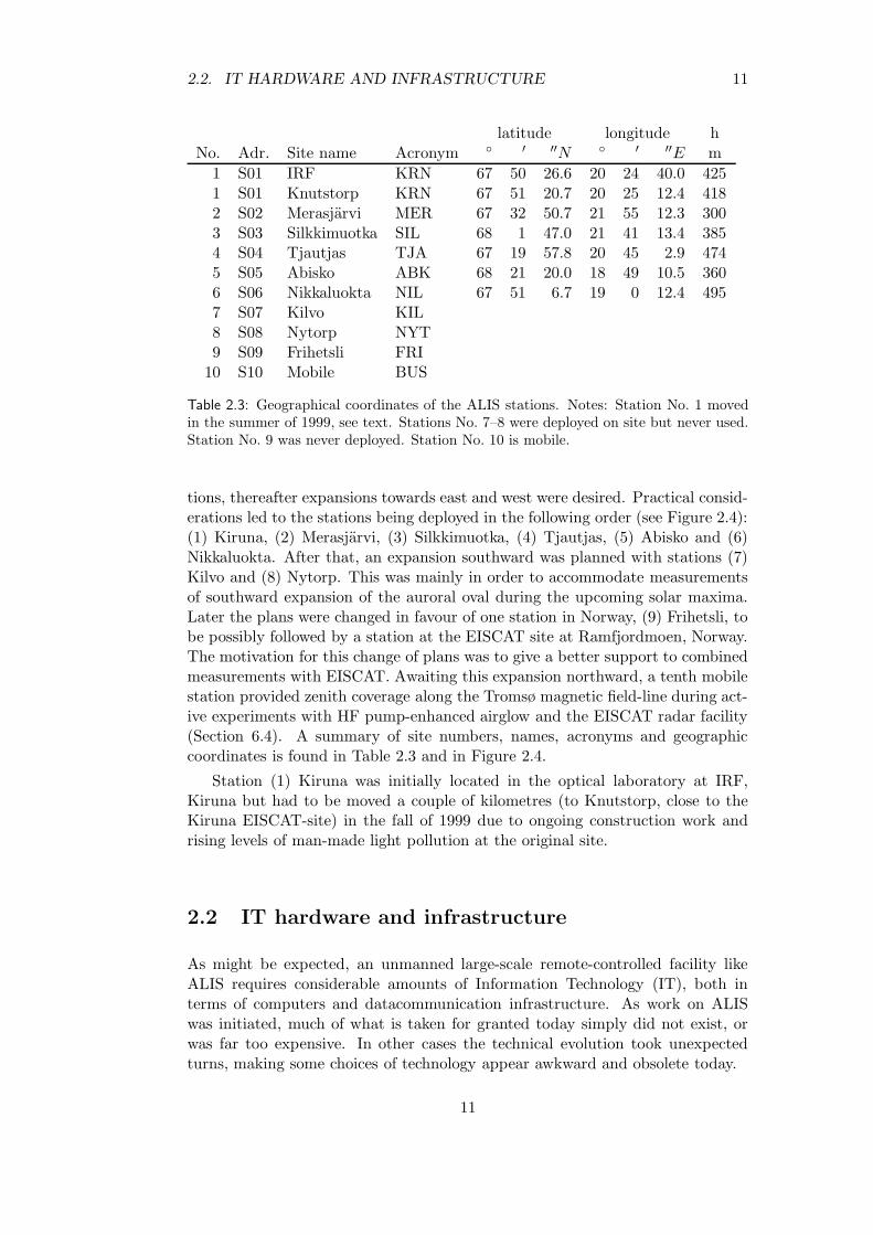
Table 2.3: Geographical coordinates of the ALIS stations. Notes: Station No. 1 movedin the summer of 1999, see text. Stations No. 7–8 were deployed on site but never used.Station No. 9 was never deployed. Station No. 10 is mobile.
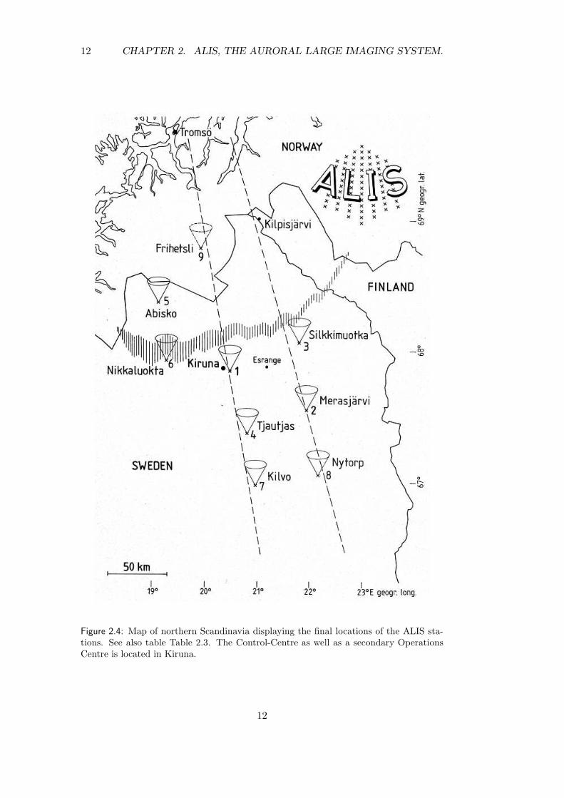
tions, thereafter expansions towards east and west were desired. Practical consid-erations led to the stations being deployed in the following order (see Figure 2.4):(1) Kiruna, (2) Merasjarvi, (3) Silkkimuotka, (4) Tjautjas, (5) Abisko and (6)Nikkaluokta. After that, an expansion southward was planned with stations (7)Kilvo and (8) Nytorp. This was mainly in order to accommodate measurementsof southward expansion of the auroral oval during the upcoming solar maxima.Later the plans were changed in favour of one station in Norway, (9) Frihetsli, tobe possibly followed by a station at the EISCAT site at Ramfjordmoen, Norway.The motivation for this change of plans was to give a better support to combinedmeasurements with EISCAT. Awaiting this expansion northward, a tenth mobilestation provided zenith coverage along the Tromsø magnetic field-line during act-ive experiments with HF pump-enhanced airglow and the EISCAT radar facility(Section 6.4). A summary of site numbers, names, acronyms and geographiccoordinates is found in Table 2.3 and in Figure 2.4.
Station (1) Kiruna was initially located in the optical laboratory at IRF,Kiruna but had to be moved a couple of kilometres (to Knutstorp, close to theKiruna EISCAT-site) in the fall of 1999 due to ongoing construction work andrising levels of man-made light pollution at the original site.
2.2 IT hardware and infrastructure
As might be expected, an unmanned large-scale remote-controlled facility likeALIS requires considerable amounts of Information Technology (IT), both interms of computers and datacommunication infrastructure. As work on ALISwas initiated, much of what is taken for granted today simply did not exist, orwas far too expensive. In other cases the technical evolution took unexpectedturns, making some choices of technology appear awkward and obsolete today.
11
12 CHAPTER 2. ALIS, THE AURORAL LARGE IMAGING SYSTEM.
Figure 2.4: Map of northern Scandinavia displaying the final locations of the ALIS sta-tions. See also table Table 2.3. The Control-Centre as well as a secondary OperationsCentre is located in Kiruna.
12
2.2. IT HARDWARE AND INFRASTRUCTURE 13
2.2.1 Computers
A variety of computer architectures and operating systems were available whenwork on ALIS started. At an early stage command and control functions were sep-arated from image processing, data storage and transmission. The first specific-ation of the computer systems for ALIS [Brandstrom and Steen, 1992] includeda main computer and a dedicated Image Processing Computer (IPC) in the con-trol centre. At the stations, one computer would be responsible for controllingthe station, while a special dedicated unit, called the Near-sensor Interface andProcessing Unit (NIPU), would handle the large amounts of data (≥ 2 Mbytes/s)created by the imagers.
A Hewlett Packard HP-755 PA-RISC workstation was selected as the con-trol centre main computer. Budgetary constraints prohibited the use of similarcomputers at the stations. Therefore it was decided to use IBM-PC compatiblemachines (i486). Due to the fast development of computer hardware, the stationcomputers have been replaced after typically 3 years of operation. The currentsystem still uses various PCs (ranging from i486 to Pentium III). At the controlcentre the HP-755 computer lasted until 1999 when it was replaced by two PCs.The aim of having a dedicated image processing computer has not been realisedas no real-time data is yet available due to the absence of high-speed lines to thestations. Dataanalysis is performed on various workstations.
2.2.2 The NIPU
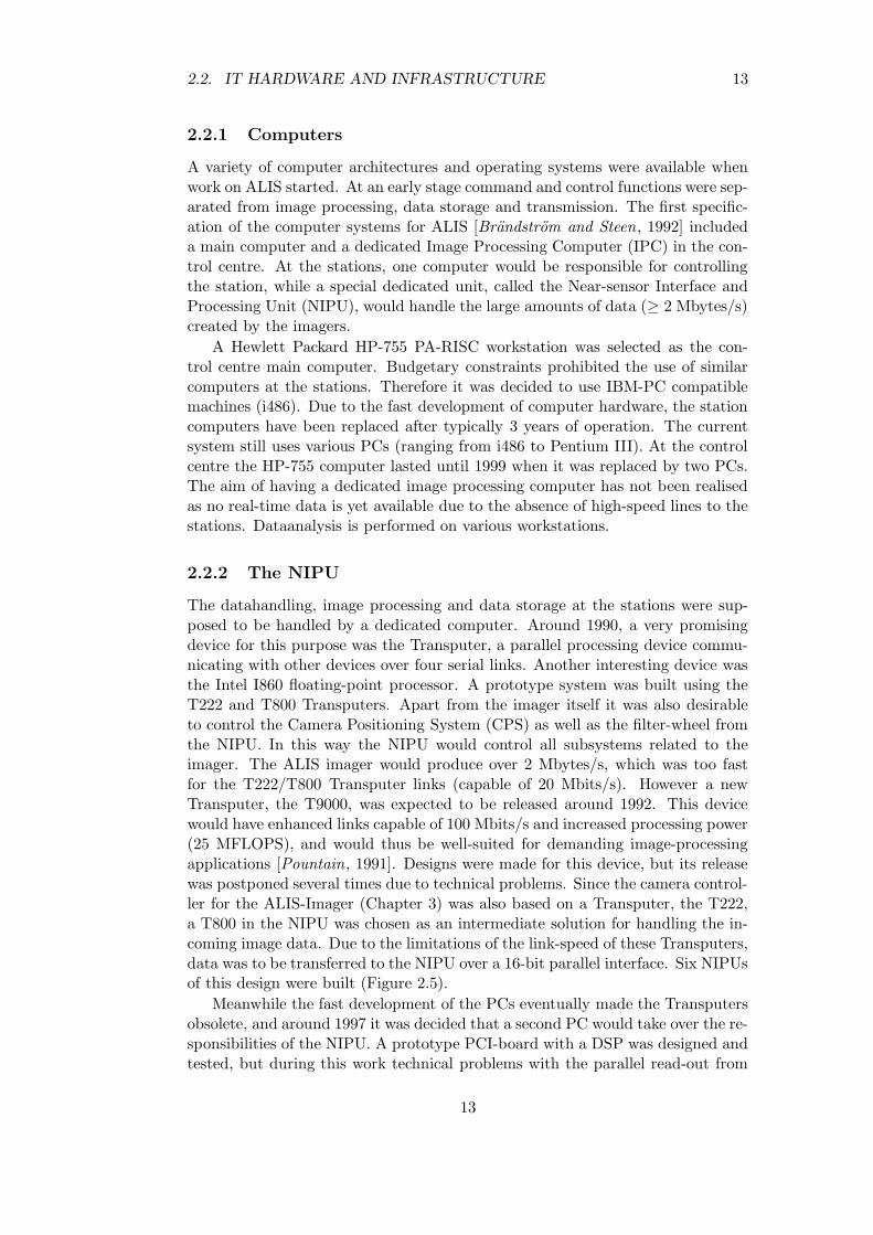
The datahandling, image processing and data storage at the stations were sup-posed to be handled by a dedicated computer. Around 1990, a very promisingdevice for this purpose was the Transputer, a parallel processing device commu-nicating with other devices over four serial links. Another interesting device wasthe Intel I860 floating-point processor. A prototype system was built using theT222 and T800 Transputers. Apart from the imager itself it was also desirableto control the Camera Positioning System (CPS) as well as the filter-wheel fromthe NIPU. In this way the NIPU would control all subsystems related to theimager. The ALIS imager would produce over 2 Mbytes/s, which was too fastfor the T222/T800 Transputer links (capable of 20 Mbits/s). However a newTransputer, the T9000, was expected to be released around 1992. This devicewould have enhanced links capable of 100 Mbits/s and increased processing power(25 MFLOPS), and would thus be well-suited for demanding image-processingapplications [Pountain, 1991]. Designs were made for this device, but its releasewas postponed several times due to technical problems. Since the camera control-ler for the ALIS-Imager (Chapter 3) was also based on a Transputer, the T222,a T800 in the NIPU was chosen as an intermediate solution for handling the in-coming image data. Due to the limitations of the link-speed of these Transputers,data was to be transferred to the NIPU over a 16-bit parallel interface. Six NIPUsof this design were built (Figure 2.5).
Meanwhile the fast development of the PCs eventually made the Transputersobsolete, and around 1997 it was decided that a second PC would take over the re-sponsibilities of the NIPU. A prototype PCI-board with a DSP was designed andtested, but during this work technical problems with the parallel read-out from
13
14 CHAPTER 2. ALIS, THE AURORAL LARGE IMAGING SYSTEM.
Figure 2.5: The NIPU. The board contains four T222 modules, each controlling the αand β axes of the camera-positioning system as well as the filter-wheel and an additionalTransputer intended (but never used) for GPS-timing. The large module is the T800-board with memory and parallel interface for image capture from the 16-bit parallelinterface of the camera controller. Ample space is provided for future expansions withT9000 boards.
14
2.2. IT HARDWARE AND INFRASTRUCTURE 15
the camera controller were discovered (Section 3.3.4). Since these problems couldnot be resolved, the resulting decrease of the maximum imager frame-rate madeboth the NIPU and the second PC for receiving image data superfluous. Thereforethe six already existing NIPUs ended up as rather over-designed controllers forthe camera-positioning system (Section 3.6) and the filter-wheels (Section 3.5.1).
2.2.3 Communication systems
When design work on ALIS began, the fastest off-the-shelf modem available wasat 2400 bits/s, and with a special, rather expensive, leased-line one could attain9600 bits/s. The first ALIS paper [Steen, 1989] specified a ≥ 10 Mbits/s com-munication link capable of near real-time image transfer to the control centre. Anetwork of microwave links was considered but deemed far too expensive, as wasthe case with the fibre-optic lines passing near two of the stations (Merasjarvi,Silkkimuotka, see below).
Dial-up telephone lines were too slow, and faster means of communication tooexpensive. It was anticipated that the fast technological development in this fieldwould make faster communication lines available at a reasonable cost. Thus itwas decided that ALIS would use slow dial-up modem lines for command, statusinformation and to transmit reduced quick-look images to the control centre.A future “to be defined” high-speed link to the control centre would providethe high-speed communication required for real-time transfer of raw image data.Meanwhile, local data storage, and on-site image processing of the data would beemployed at the stations.
The dial-up lines were one of the major sources of trouble in ALIS duringthe early years. This was mainly due to bad telephone lines and old electro-mechanical telephone switching equipment. This led to extensive efforts to trou-bleshoot modem lines and to develop reliable communications software. Also themodem technology and quality of the telephone lines improved considerably overthe years. Today the dial-up lines are capable of reliable 28800 bits/s communic-ation, using the standard Point-to-Point Protocol (ppp) [Simpson, 1994].
The high-speed link remains to be defined. The optimal solution would beoptical fibres (> 100 Mbits/s), but other solutions are also possible, such as ADSL(500 kbits/s), ISDN (< 128 kbits/s), radio-links (> 1 Mbits/s), etc.
Stations (2) Merasjarvi and (3) Silkkimuotka are located in the proximity ofnodes for high bandwidth fibre-optic communication lines. (5) Abisko is locatedclose to the Abisko Scientific Station (ANS) which recently acquired high-speedfibre optic Internet connection.
Presently only the Kiruna station has a 2 Mbits/s Ethernet connection toInternet realised by a microwave-link to IRF, the rest of the stations are connectedby means of 28 kbits/s dial-up modem lines. The rapidly increasing demand forhigh-speed Internet subscriptions among the general public might speed up theprocess of getting faster communication lines for all ALIS stations at a reasonablecost.
15

16 CHAPTER 2. ALIS, THE AURORAL LARGE IMAGING SYSTEM.
2.2.4 Station data storage
Various solutions for the local data storage at the stations have been consideredover the years. Initially it was intended to store the image data onto Digital DataStorage (DDS) tapes which around 1992 had a storage capacity of up to 1 Gbyte.However, this solution proved slow and unreliable, mainly due to the hostile envir-onment at the stations during tape-changes (moist, rapid temperature changes,etc.). Other solutions were also studied, but most of these were too complic-ated, too expensive or both. If faster communications would have been available,data could be stored on hard-disks, and downloaded to the control-centre in nearreal-time, or during non-measuring time. As the DDS drives tested at the firststations were not as reliable as expected, large (i.e. 2–9 Gbytes around 1992)external SCSI hard-disks were used instead. When a disk became full, it wasexchanged manually, either by neighbours to the stations, or by staff from IRF.This solution proved simple and reliable. The only disadvantage was the usuallyrather long time (typically months) before raw-data from all stations becameavailable for archiving and analysis.
2.2.5 Data archiving and availability
Reduced quick-look images (about 16 kBytes) are transmitted to the controlcentre and distributed to the operations centre (and web-site) in near real-timeduring measurement. However, these images are only intended for monitoring,and are of far too poor resolution for scientific analysis.
As the raw-data disks reach the control centre, recordable CDs (CD-R) ofALIS data are produced, and archived. All ALIS data produced so far are alsomade freely available on the world-wide web (see http://www.alis.irf.se fordetails) The main archive web-site is maintained by Peter Rydesater who alsoprovides a SQL database and search tools (see also Section 6.2).
The image data is stored in the Flexible Image Transfer System (FITS),[NASA, 1999]. This format is in wide use by the astronomical community, andfound to be particularly suited to store scientific image data, as all supplementaryinformation regarding an image (exposure time, filter, CCD temperatures, sub-sequent processing etc.) can be stored in the image header in a flexible way. FITSis recognised by many image processing packages, and free conversion programsto most other image formats exist on the Internet for most operating systems.
The size of the image-files is 16 bits/pixel (2 bytes) where the number of pixelsis dependent on the configured spatial resolution (see Table 2.2 and Section 3.2).The total size of a set of images is also dependent on the number of stationsinvolved and the temporal resolution selected.
2.2.6 Operating Systems
It was an early requirement to have a true multi-tasking operating system suchas Unix for ALIS. HP-UX, which was delivered with the workstation selectedfor the control centre fulfilled this demand. The decision to use the IBM-PCarchitecture at the stations limited the choice of operating systems to SCO-Unixand MS-DOS. SCO-Unix was quite expensive compared to its reliability, so the
16
2.3. THE ALIS CONTROL CENTRE 17
reluctantly chosen remaining option was to use MS-DOS at the stations. Thislead to limitations in the flexibility of the system.
Some years later highly reliable and free operating systems such as Free-BSDand GNU/Linux emerged. It was immediately realised that a change to one ofthese operating systems at the stations would be necessary to meet the requireddata-handling specifications. In 1997 all stations had changed operating systemsto Debian GNU/Linux, and in the fall of 1999 the HP-UX operating system inthe control centre was also changed to GNU/Linux as the old HP workstationwas replaced.
2.3 The ALIS control centre
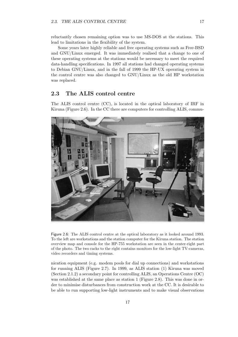
The ALIS control centre (CC), is located in the optical laboratory of IRF inKiruna (Figure 2.6). In the CC there are computers for controlling ALIS, commu-
Figure 2.6: The ALIS control centre at the optical laboratory as it looked around 1993.To the left are workstations and the station computer for the Kiruna station. The stationoverview map and console for the HP-755 workstation are seen in the center-right partof the photo. The two racks to the right contains monitors for the low-light TV-cameras,video recorders and timing systems.
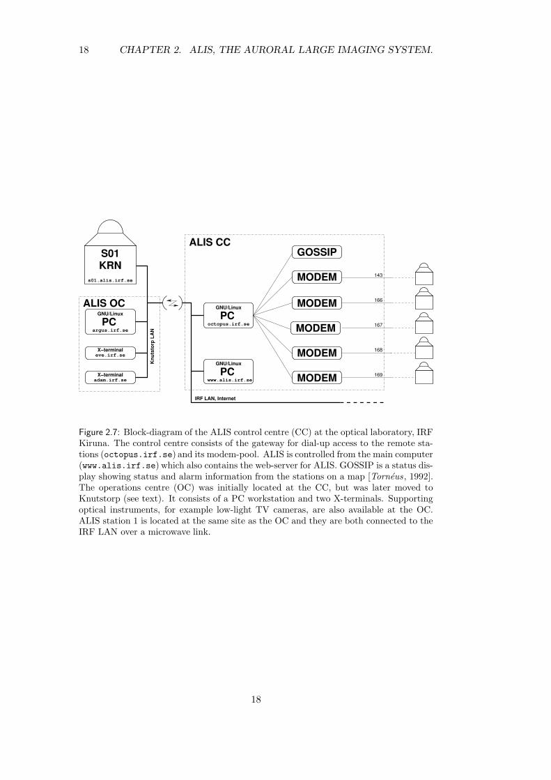
nication equipment (e.g. modem pools for dial up connections) and workstationsfor running ALIS (Figure 2.7). In 1999, as ALIS station (1) Kiruna was moved(Section 2.1.2) a secondary point for controlling ALIS, an Operations Centre (OC)was established at the same place as station 1 (Figure 2.8). This was done in or-der to minimise disturbances from construction work at the CC. It is desirable tobe able to run supporting low-light instruments and to make visual observations
17
18 CHAPTER 2. ALIS, THE AURORAL LARGE IMAGING SYSTEM.
MODEM
MODEM
MODEM
MODEM
MODEM
GOSSIP
PCGNU/Linux
X−terminal
X−terminal
PCGNU/Linux
s01.alis.irf.se
S01KRN
PCGNU/Linux
168
143
166
167
169
octopus.irf.seargus.irf.se
adam.irf.se
eve.irf.se
www.alis.irf.se
ALIS OC
ALIS CC
IRF LAN, Internet
Knu
tsto
rp L
AN
Figure 2.7: Block-diagram of the ALIS control centre (CC) at the optical laboratory, IRFKiruna. The control centre consists of the gateway for dial-up access to the remote sta-tions (octopus.irf.se) and its modem-pool. ALIS is controlled from the main computer(www.alis.irf.se) which also contains the web-server for ALIS. GOSSIP is a status dis-play showing status and alarm information from the stations on a map [Torneus , 1992].The operations centre (OC) was initially located at the CC, but was later moved toKnutstorp (see text). It consists of a PC workstation and two X-terminals. Supportingoptical instruments, for example low-light TV cameras, are also available at the OC.ALIS station 1 is located at the same site as the OC and they are both connected to theIRF LAN over a microwave link.
18
2.3. THE ALIS CONTROL CENTRE 19
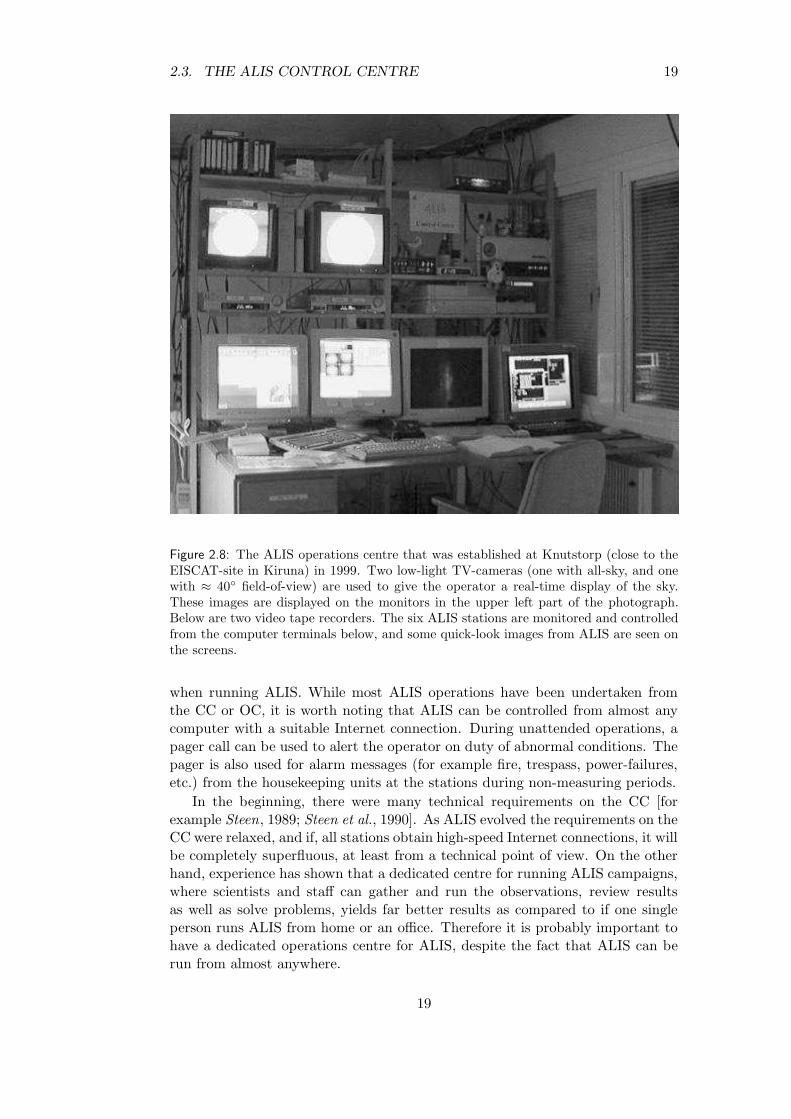
Figure 2.8: The ALIS operations centre that was established at Knutstorp (close to theEISCAT-site in Kiruna) in 1999. Two low-light TV-cameras (one with all-sky, and onewith ≈ 40 field-of-view) are used to give the operator a real-time display of the sky.These images are displayed on the monitors in the upper left part of the photograph.Below are two video tape recorders. The six ALIS stations are monitored and controlledfrom the computer terminals below, and some quick-look images from ALIS are seen onthe screens.
when running ALIS. While most ALIS operations have been undertaken fromthe CC or OC, it is worth noting that ALIS can be controlled from almost anycomputer with a suitable Internet connection. During unattended operations, apager call can be used to alert the operator on duty of abnormal conditions. Thepager is also used for alarm messages (for example fire, trespass, power-failures,etc.) from the housekeeping units at the stations during non-measuring periods.
In the beginning, there were many technical requirements on the CC [forexample Steen, 1989; Steen et al., 1990]. As ALIS evolved the requirements on theCC were relaxed, and if, all stations obtain high-speed Internet connections, it willbe completely superfluous, at least from a technical point of view. On the otherhand, experience has shown that a dedicated centre for running ALIS campaigns,where scientists and staff can gather and run the observations, review resultsas well as solve problems, yields far better results as compared to if one singleperson runs ALIS from home or an office. Therefore it is probably important tohave a dedicated operations centre for ALIS, despite the fact that ALIS can berun from almost anywhere.
19

20 CHAPTER 2. ALIS, THE AURORAL LARGE IMAGING SYSTEM.
20
21
Chapter 3
The ALIS Imager
“For now we see through a glass, darkly; but then face to face: now I knowin part; but then shall I know even as also I am known.” 1 Cor. 13:12
“Orten, hvarifran de [Norr-skenen] askadas; tiden da de visa sig; deras sta-llning pa himmelen; ombyteliga figur och vackra fargor; aro nastan de endeomstandligheter, som darvid, afven med svarighet, kunna i akt tagas. Ogat,pennan och den snallaste Malares pensel, aro for senfardige, att teckna alladeras forandringar. Deras fladdrande ombyten forvilla imaginationen, ochman bor vara god geometra, at skilja utseendet och figuren ifran sjalva ting-en, for at ej med allmanheten och forntiden daraf tillskapa tusende syneroch vidunder, uti blotta luften.” Wilcke [1778]
Spectroscopic measurements of auroral and airglow emissions have belonged tothe realm of photometer measurements, while imaging techniques mainly havebeen tools for studies of morphology and dynamics. This chapter will discussthe required specifications for the ALIS imager in order to enable absolute spec-troscopic measurements of column emission rates. Calibration issues will be dis-cussed in Chapter 4.
3.1 Some basic concepts
There exist a number of textbooks [for example Theuwissen, 1995; Holst , 1998,and references therein], reports [for example Eather , 1982; Lance and Eather ,1993], and articles [for example Janesick et al., 1987, and references therein] onsolid-state imaging with CCD detectors. This section will provide a short sum-mary of some fundamental concepts required to specify a CCD-imaging systemsuitable for the needs of auroral and airglow imaging.
Holst [1998] defines the term radiometry, as the “energy or power transferfrom a source to a detector” while photometry is defined as “the transfer froma source to a detector where the units of radiation have been normalised to thespectral sensitivity of the eye.”
3.1.1 Spectral radiant sterance (radiance)
The basic quantity from which all other radiometric quantities can be derived isspectral radiant sterance, L. Given a source area, As, radiating a radiant flux,
21
22 CHAPTER 3. THE ALIS IMAGER
Φ, into a solid angle, Ω. The spectral radiant sterance in energy units, LE, thenbecomes:
LE(λ) =∂2Φ(λ)
∂As∂Ω
[
W
m2 sr
]
(3.1)
where λ is the wavelength. Expressing the spectral radiant sterance in quantumunits (Lγ) the following equation is obtained:
Lγ =LE
hν=
LEλ
hc
[
photons
s m2 sr
]
(3.2)
Here ν is the frequency, h is Planck’s constant and c is the speed of light. Pleasenote spectral radiant sterance (radiance) is not to be confused with surface bright-ness which is a photometric unit involving the characteristics of the human eye[see Holst , 1998, pp. 20,26].
3.1.2 The Rayleigh
In terms of measurement techniques the aurora can be regarded as a five-dim-ensional signal with three spatial dimensions, one temporal and one spectraldimension. The desired physical quantity is usually the volume emission rate,ε(r, t, λ), which cannot be found directly from measurements. However the rateof emission from a 1 m2 column along the line of sight is normally just 4πLγ forany isotropic source with no self-absorption [Hunten et al., 1956].
Consider a cylindrical column of cross-sectional area 1 m2 extending awayfrom the detector into the source. The volume emission rate from a volumeelement of length dl at distance l is ε(l, t, λ) photons m−3 s−1. The contributionto Lγ is given by:
dLγ =ε(l, t, λ)
4πdl
[
photons
s m2 sr
]
(3.3)
Integrating along the line of sight, l :
4πLγ =
∫ ∞
0ε(l, t, λ)dl (3.4)
This quantity is the column emission rate, which Hunten et al. [1956] proposedas a radiometric unit for the aurora and airglow. (See also Chamberlain [1995,App. II]) The unit is named after the fourth Lord Rayleigh, R. J. Strutt, 1875–1947, who made the first measurements of night airglow [Rayleigh, 1930]. (Not tobe confused with his father, J. W. Strutt, 1842–1919 remembered for Rayleigh-scattering etc.) In SI-units the Rayleigh becomes [Baker and Romick , 1976]:
1 [Rayleigh] ≡ 1 [R] , 1010
[
photons
s m2 column
]
(3.5)
The word column denotes the concept of an emission-rate from a column ofunspecified length, as discussed above. It should be noted that the Rayleighis an apparent emission rate, not taking absorption or scattering into account.However, Hunten et al. [1956] emphasise that “the Rayleigh can be used as definedwithout any commitment as to its physical interpretation, even though it has been
22
3.1. SOME BASIC CONCEPTS 23
chosen to make interpretation convenient.” The spectral radiant sterance (Lγ)in Equation 3.2 can be obtained from the column emission rate I (in Rayleighs)according to Baker and Romick [1976]:
Lγ =1010I
4π
[
photons
s m2 sr
]
(3.6)
Although not a proper SI-unit, the Rayleigh is often used in the field of auroraland airglow measurements. It is also frequently misunderstood and abused. It isimportant to remember that the Rayleigh only is usable when the wavelength isspecified. Due to the plethora of Rayleigh definitions [Baker and Romick , 1976],it is always wise to state the definition of the unit before using it. In the followingtext, the Rayleigh will be used according to the original definition [Hunten et al.,1956, but in SI-units] as defined above.
Using the recommended column emission rates in Rayleighs for the Interna-tional Brightness Coefficients (IBC) as an example, the following spectral radiantsterances are obtained [Chamberlain, 1995, App. II]: IBC-I aurora, correspondingto 1 kR at 5577 A is often described as the lowest column emission rate detectableby the unaided human eye. Usually this is compared to the luminous incidence ofa moonless cloudy night which is about 10−4 Lux∗. By the use of Equations 3.2and 3.6, the spectral radiant sterance in energy units (LE) can be calculated:
LE(1 [kR]) =1013hc
4πλ=
103hc
4π × 5577≈ 300
[
nW
s m2 sr
]
(3.7)
Similarly the brightest IBC-IV corresponding to 1 MR at 5577 A, which is oftencompared to the luminous incidence of the full-moon of about 10−1 Lux∗ becomes:
LE(1 [MR]) ≈ 300
[
µW
s m2 sr
]
(3.8)
3.1.3 Spectral radiant incidence (irradiance)
Spectral radiant incidence (irradiance), E, is defined as radiant power incidentper unit area onto a target, in this case typically the effective aperture of theoptics, Aapp, image area, Ai, area of CCD-detector, ACCD, or the area of a CCDpixel, Apix.
The transmittance, T (λ, ...), of an optical system is a function of many para-meters, for example wavelength λ, viewing angle, temperature, etc., and must beexperimentally determined (See Chapter 4). Here it is enough to state that thetotal transmittance is given by the product of the individual transmittances ofthe various components of the optical system:
T =∏
∀X
TX = TaToTf . . . (3.9)
Where TX is exemplified by Ta, To and Tf which are the transmittance of theatmosphere, optics and filter, respectively. In the following text T will denotethe product of appropriate transmittances according to Equation 3.9.
∗According to Holst [1998, p. 28]
23
24 CHAPTER 3. THE ALIS IMAGER
Consider an extended source of area, As, of given column emission rate, I,imaged by an optical system, here represented by a single lens with given focallength, f , and f-number, f#. The relation between the aperture-stop, dapp, f andf# is given by:
f# =f
dapp(3.10)
Setting the source at distance rs from the lens, which is at the distance ri fromthe detector and letting Ωds be the solid angle of the lens aperture as seen fromthe source, (assuming small angles), the photon flux, Φγapp , at the lens aperturethen becomes:
Φγapp = LγAsTaΩds = LγAsTaAapp
r2s
[
photons
s
]
(3.11)
The spectral radiant incidence at the aperture, Eγapp , then becomes:
Eγapp =Φγapp
Aapp=
LγAsTa
r2s
[
photons
s m2
]
(3.12)
The spectral radiant incidence at the image plane, Eγi, is given by (by substitut-
ing Equation 3.10 and assuming a circular aperture):
Eγi=
Φγapp
Ai= Lγ
As
AiT
πd2app
4r2s
= LγAs
AiT
πf2
4r2sf
2#
= LγAs
AiT
πf2
4r2sf
2#
[
photons
s m2
]
(3.13)Noting that, for thin lenses and small angles:
1
rs+
1
ri=
1
f(3.14)
In this case:rs ri ⇒ ri ≈ f (3.15)
The lens-magnification formula is:
M2 =
(
hi
hs
)2
=Ai
As=
(
ri
rs
)2
(3.16)
where hi and hs denote the height of the image and source respectively. InsertingEquations 3.6 and 3.14-3.16 into Equation 3.13, the following equation for Eγi
isobtained:
Eγi=
TΦγ
Ai= TLγ
π
4f2#
= T1010I
16f2#
[
photons
s m2
]
(3.17)
Note that this equation is only accurate for small angles, an off-axis image willhave reduced incidence compared to an on-axis image. This is called the “naturalvignetting”, cos4 θ, and is usually inserted as a multiplication factor in Equa-tion 3.17, as required.
However, the actual vignetting is highly dependent on the characteristics ofthe optical system. Therefore the vignetting as well as other aberrations, and thetransmittance (T ) must be experimentally determined. This will be consideredfurther in Chapter 4 and references therein.
24
3.1. SOME BASIC CONCEPTS 25
3.1.4 Number of incident photons
Using Equation 3.17 the number of photons reaching the image plane, nγi, can
be calculated:
nγi= Eγi
tintAi = T tintAi1010I
16f2#
[photons] (3.18)
Here tint is the integration time in seconds. The number of photons hitting theCCD, nγCCD
, are:
nγCCD= nγi
TwTCCDACCD
Ai[photons] (3.19)
Here Tw is the transmittance of the optical window protecting the CCD, andTCCD is the transmittance of the CCD substrate (in the case of a back-sideilluminated CCD). Likewise, the number of photons hitting an individual pixel,nγpix
, is:
nγpix= nγCCD
Apix
ACCD= T tintApix
1010I
16f2#
[photons] (3.20)
(using Equations 3.18–3.19 and Equation 3.20). Again, please remember thecaution at the end of Section 3.1.3
3.1.5 The CCD as a scientific imaging detector
“During the past couple of decades the Charge Coupled Device (CCD) sensorhas gradually replaced the tube type sensors, such as the vidicon, due to itsadvantages in size, weight, power consumption, noise characteristics, linearity,dynamic range, photometric accuracy, spectral responsitivity, geometric stability,reliability, and durability” [Janesick et al., 1987]. As an auroral imager, theCCD is thus almost an ideal detector for ground-based as well as for space-borneinstruments. The CCD can be used either as the primary photon detector, or inan Intensified CCD (ICCD) configuration. Whether to use a CCD or an ICCD ismainly a matter of requirements on temporal resolution and signal-to-noise ratio,SNR. This section will begin with a short review of a number of parametersdescribing the performance of a CCD detector.
3.1.6 Quantum efficiency
The quantum efficiency, QE , is a measure of the number of electrons generatedper incident photon:
QE = ηEQEI
[
e−
photons
]
(3.21)
where ηE is the effective quantum yield (electrons generated, collected, and trans-ferred per interacting photon per pixel) and QEI is the interacting quantum effi-ciency (interacting photons per incident photons per pixel) [Janesick et al., 1987].However, for the purpose of this text it is only needed to consider QE , which forthe purpose of this text, is the same as the detective quantum efficiency (DQE).
Quantum efficiency for a CCD is wavelength dependent, and is of no valueunless the wavelength is specified. High performance scientific thinned, back-side illuminated anti-reflection coated CCD devices might have as high quantum
25
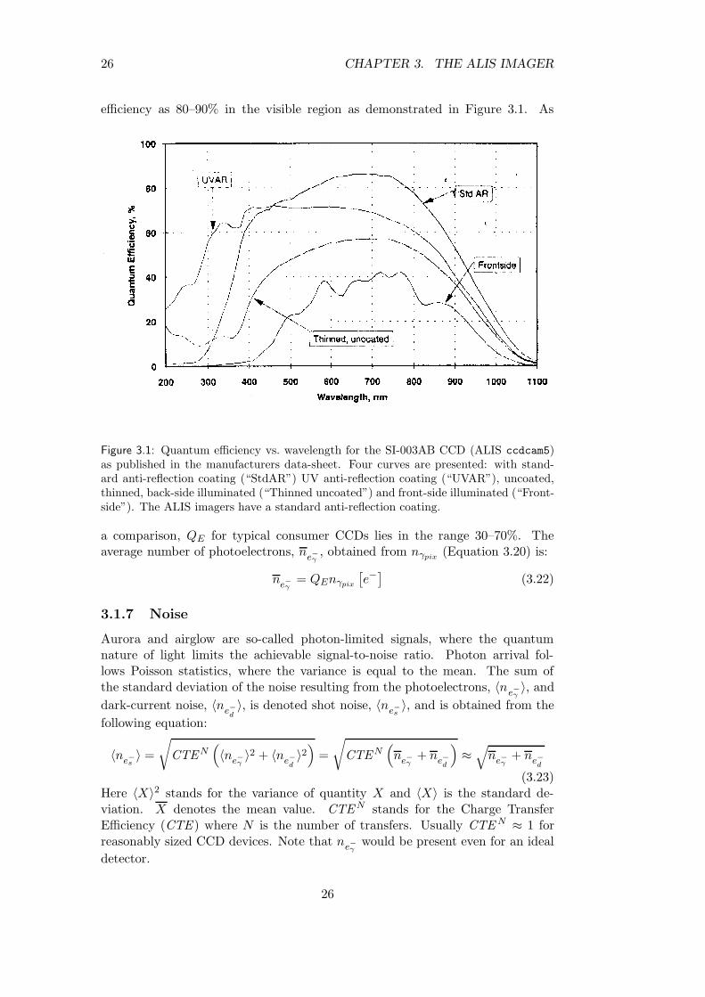
26 CHAPTER 3. THE ALIS IMAGER
efficiency as 80–90% in the visible region as demonstrated in Figure 3.1. As
Figure 3.1: Quantum efficiency vs. wavelength for the SI-003AB CCD (ALIS ccdcam5)as published in the manufacturers data-sheet. Four curves are presented: with stand-ard anti-reflection coating (“StdAR”) UV anti-reflection coating (“UVAR”), uncoated,thinned, back-side illuminated (“Thinned uncoated”) and front-side illuminated (“Front-side”). The ALIS imagers have a standard anti-reflection coating.
a comparison, QE for typical consumer CCDs lies in the range 30–70%. Theaverage number of photoelectrons, n
e−γ, obtained from nγpix
(Equation 3.20) is:
ne−γ
= QEnγpix
[
e−]
(3.22)
3.1.7 Noise
Aurora and airglow are so-called photon-limited signals, where the quantumnature of light limits the achievable signal-to-noise ratio. Photon arrival fol-lows Poisson statistics, where the variance is equal to the mean. The sum ofthe standard deviation of the noise resulting from the photoelectrons, 〈n
e−γ〉, and
dark-current noise, 〈ne−d〉, is denoted shot noise, 〈n
e−s〉, and is obtained from the
following equation:
〈ne−s〉 =
√
CTEN(
〈ne−γ〉2 + 〈ne−
d〉2
)
=
√
CTEN(
ne−γ+ ne−
d
)
≈√
ne−γ+ ne−
d
(3.23)Here 〈X〉2 stands for the variance of quantity X and 〈X〉 is the standard de-viation. X denotes the mean value. CTEN stands for the Charge TransferEfficiency (CTE ) where N is the number of transfers. Usually CTE N ≈ 1 forreasonably sized CCD devices. Note that ne−γ
would be present even for an ideal
detector.
26
3.1. SOME BASIC CONCEPTS 27
Additional noise sources include: reset noise, on-chip and off-chip amplifiernoise (1/f-noise and white noise). Of particular interest for low-light applicationsis that the 1/f-noise, which is the main source of the read noise (“noise-floor”), in-creases in proportion to the square root of the read-out frequency (“pixel-clock”),thus requiring a suitable compromise between noise performance and frame-rate.The analogue-to-digital converter has a quantisation noise, also switching transi-ents coupled through the clock signals, electro-magnetic interference, etc., sumsup to the total noise. There is pattern noise due to differences in dark-currentand photo response non-uniformities [Holst , 1998]. At high signal levels the totalnoise is dominated by pattern noise (pixel to pixel sensitivity variations withinthe CCD) for most CCDs, at low signal levels the read noise (“noise floor”) dom-inates [Janesick et al., 1987]. Many of these noise sources can be reduced to neg-ligible levels by good electronic design practices. In particular, the dark-current(and reset noise) is reduced by cooling the CCD. By the use of Double CorrelatedSampling (DCS) the reset noise can be almost eliminated. The quantisation noiseis eliminated by using a sufficiently high resolution ADC. It is, however, beyondthe scope of this work to embark onto a detailed analysis of the noise-sources inCCD imagers, instead a simplified noise model from Holst [1998] is adopted:
〈ne−CCD
〉 =√
〈ne−s〉2 + 〈ne−r
〉2 + 〈ne−p〉2
[
e−RMS
]
(3.24)
The standard deviation of the noise floor (or read noise), 〈ne−r〉, is usually stated in
the imager specification as ‘read noise’, or easily obtained from a zero exposure.This noise source increases with the square-root of the pixel clock frequency,which imposes an SNR constraint onto the frame-rate.
The pattern noise, 〈ne−p〉, is the sum of Fixed Pattern Noise (FPN), result-
ing from pixel-to-pixel variations in the dark-current, and Photo Response Non-Uniformities (PRNU). An approximate worst case value is provided by Holst[1998]:
〈ne−p〉 =
√
〈ne−FPN
〉2 + 〈ne−PRNU
〉2 ≈ 〈ne−PRNU
〉 ≈ Une−γ≈
ne−γ√ne−max
[
e−RMS
]
(3.25)However, for the low signal levels considered here, pattern noise is neglected.Then the total noise approximation for a bare CCD becomes (by substitutingEquation 3.23 into Equation 3.24):
〈ne−CCD
〉 ≈√
ne−γ
+ ne−d
+ 〈ne−r〉2
[
e−RMS
]
(3.26)
It should be remembered that this equation is an approximation.
3.1.8 Signal-to-noise ratio
The measured signal-to-noise ratio in terms of the digital output, DN , or in termsof root-mean-square electrons e−RMS is defined as follows:
SNRCCD =DN signal
DN noise≈
ne−γ
〈ne−CCD
〉 (3.27)
27
28 CHAPTER 3. THE ALIS IMAGER
Substituting Equation 3.26 the SNR can now be calculated with the help ofEquations 3.20 and 3.22 and the total noise is given by Equation 3.26:
SNRCCD ≈n
e−γ√
ne−γ
+ ne−d
+ 〈ne−r〉2
(3.28)
For an ideal photon detector Equation 3.28 becomes:
SNRγideal =√
ne−γ
(3.29)
3.1.9 The signal-to-noise ratio of an ICCD
In the image-intensifier, for each primary photoelectron emitted by the photo-cathode (pc), the image-intensifier produces a burst of approximately 103 second-ary CCD electrons, typically by the use of a micro-channel plate (MCP) betweenthe photo-cathode and phosphor screen. The phosphor screen is then opticallycoupled to the CCD by the use of lenses or a fibre-optic taper†.
The number of photons reaching the image plane (nγi) is given by Equa-
tion 3.18. The average number of signal electrons generated by the photo-cathode,ne−γ,pc
, for a pixel area Apix projected onto the photo-cathode, by the fibre-optic
minification ratio, MFO is given by [see Holst , 1998, p. 196]:
ne−γ,pc
= QEpcne−γi
Apix
Ai= QEpcT tintM
2FOApix
1010I
16f2#
[
e−RMS
]
(3.30)
After the MCP the number of electrons are amplified with the average MCPgain, g, i.e. average number of secondary photoelectrons, ne−
γMCP, produced per
photo-cathode electron ne−γ,pc
ne−γMCP
= g ne−γ,pc
[
e−RMS
]
(3.31)
The photoelectrons are then converted back to photons by the phosphor screenwith a phosphor efficiency, ηP , and then re-imaged onto the CCD via a fibre optictaper. The transmittance losses here are denoted TFO. Finally the photons hitthe CCD and are converted to photoelectrons:
ne−γCCD
= ηP QECCDTFO n
e−γMCP
[
e−RMS
]
(3.32)
By applying the following approximation:
QEICCD= QEpcηPQECCD
TFO ≈ QEpc
the following equation is obtained (using Equations 3.30-3.32):
ne−γCCD
= g ne−γ,pc
= g QEpcT tintM2FOApix
1010I
16f2#
[
e−RMS
]
(3.33)
†In this text, the term “ICCD” is used for the combination of an image intensifier and aCCD, regardless of coupling type, or if they are manufactured as one unit or not.
28

3.1. SOME BASIC CONCEPTS 29
As with the CCD (see Equation 3.23), the photo-cathode produces both photon-noise and dark-current noise :
〈ne−s,pc〉 =
√
〈ne−γ,pc〉2 + 〈ne−
d,pc〉2
[
e−RMS
]
(3.34)
Another noise source, unique to the ICCD, is the electron multiplication noise,which is due to the statistical distribution of the number of secondary photoelec-trons‡. Taking this uncertainty in g into account, the combined variance withthe photon noise becomes:
〈ne−γ,pc〉2 = kMCP g2 ne−γ,pc
≈ 2g2 ne−γ,pc(3.35)
Here, kMCP is the microchannel excess noise. The photo-cathode dark-currentnoise, is also dependent on g in the same way:
〈ne−d,pc
〉2 = 2g2 ne−d,pc
(3.36)
Taking Equation 3.26 as an approximation for the total CCD noise, and in-serting into it Equations 3.35 and 3.36, for the ICCD noise sources, leads to thefollowing expression for the total noise for the ICCD, 〈n
e−ICCD
〉 :
〈ne−ICCD
〉 ≈√
2g2 (ne−γ,pc+ ne−
d,pc) + ne−
d+ ne−r
(3.37)
By applying Equations 3.33 and 3.37 into Equation 3.27 the following approxim-ation for the SNR of an ICCD, SNRICCD, emerges:
SNRICCD ≈g n
e−γ,pc√
2g2 (ne−γ,pc+ ne−
d,pc) + ne−
d+ ne−r
(3.38)
As seen, increasing the gain of the image intensifier makes the CCD noise-sourcesnegligible, but does not increase the SNR. For very high gain, Equation 3.38 isreduced to:
SNRICCD ≈ne−γ,pc
√
2(ne−γ,pc+ ne−
d,pc)
(3.39)
3.1.10 Threshold of detection and maximum signal
The threshold of detection is usually defined as SNR = 2 while the Noise Equi-valent Exposure, NEE , is obtained when SNR = 1. The maximum signal, orSaturation Equivalent Exposure (SEE) is obtained when the charge well capa-city, ne−max
, is reached. This occurs when:
ne−γ≥ ne−max
− ne−d
(3.40)
In most cases the maximum charge-well capacity, DN SEE, is matched to themaximum ADC output DN max. For the ICCD case, apart from the conditionabove, there is also a saturation level for the image intensifier to be considered.On the other hand, the high-voltage for the intensifier can be gated, acting likean electronic shutter.
‡A more detailed discussion of this noise source is found in works by Holst [1998, pp. 195–200],Trondsen [1998, p. 48], Csorba [1985, pp. 120–124] and Hertel [1989].
29
30 CHAPTER 3. THE ALIS IMAGER
3.1.11 Dynamic range
The Dynamic Range, DR, is defined as the peak signal divided by the RMS noiseand the DC-bias-level, DN DC , (if any). The minimum ADC output, DN min, issubtracted in the case of a signed integer output. DR is usually expressed indecibels.
DR = 20 log10
(
DN SEE − DN min
DN DC + DN NEE − DN min
)
[dB] (3.41)
An approximate theoretical value for DR is obtained by dividing the maximumsignal (Equation 3.40) by the total noise, 〈ne−tot
〉, which is found in Equations 3.26
and 3.37 for the CCD and ICCD case respectively.)
DR ≈ 20 log10
ne−max− ne−
d
〈ne−tot〉 [dB] (3.42)
3.2 Selecting an imager for ALIS
The selection process for an ALIS imager includes many considerations of sci-entific, technical as well as of an economical nature. Naturally this leads tovarious compromises. A complete ALIS imager consists of optics, filters and adetector with its electronics and supporting systems. The choice of detector de-termines many parameters of the other imager subsystems, therefore this choicewill be discussed first.
3.2.1 Comparison of an ICCD with a CCD imager
An ICCD imager was considered early on in the ALIS project [for example Steenet al., 1990] and indeed many excellent CCD imagers for aurora and airglow, as,for example, the HAARP imager [Lance and Eather , 1993], the Portable AuroralImager (PAI) [Trondsen, 1998] and the new Finnish all-sky camera [Syrjasuo,2001] as well as some of the imagers operated by Kaila [2003a] are based on animage-intensified CCD. Yet, it is important to realise that most CCDs have ahigher QE than that of the photo-cathode in an image-intensifier. For example,the PAI, used for high spatial and temporal resolution auroral imaging, have aQECCD
of 67 %, while the quantum efficiency of the photo-cathode is only 28%,both at λ = 5577 A [Trondsen, 1998, p. 51]. Scientific grade CCDs might have aQECCD
of up to about 90% as demonstrated in Figure 3.1. Despite this a CCDis not always preferable to an ICCD.
Figure 3.2 plots SNR as a function of column emission rate, with f# = 3.9and a fixed integration time of 16.7 ms (NTSC video standard). The CCD datawere taken from the technical specifications for the PAI (Table 3.1) as well asfrom the specifications for an ALIS imager (ccdcam5, Table 3.2). Ideal photondetectors with the same pixel area as of the ALIS Imager (a) and the PAI (c),have thresholds of detection at approximately 20 kR and 40 kR respectively. TheALIS Imager, curve (b), reaches SNR = 2 at about 100 kR which is also the casefor the PAI ICCD (d). Curve (e) for the unintensified CCD of the PAI (withoutimage intensifier) does not reach SNR = 2 until at approximately 2 MR. Clearly,
30
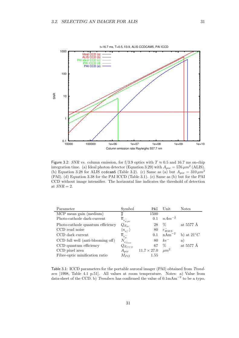
3.2. SELECTING AN IMAGER FOR ALIS 31
0.1
1
10
100
1000
10000 100000 1e+06 1e+07 1e+08 1e+09 1e+10
SN
R
Column emission rate Rayleighs 557.7 nm
t=16.7 ms, T=0.5, f/3.9, ALIS CCDCAM5, PAI ICCD
Ideal CCD (a)ALIS CCD (b)
PAI ideal CCD (c)PAI ICCD (d)PAI CCD (e)
Figure 3.2: SNR vs. column emission, for f/3.9 optics with T ≈ 0.5 and 16.7 ms on-chipintegration time. (a) Ideal photon detector (Equation 3.29) with Apix = 576 µm2 (ALIS).(b) Equation 3.28 for ALIS ccdcam5 (Table 3.2). (c) Same as (a) but Apix = 310 µm2
(PAI). (d) Equation 3.38 for the PAI ICCD (Table 3.1). (e) Same as (b) but for the PAICCD without image intensifier. The horizontal line indicates the threshold of detectionat SNR = 2.
Parameter Symbol PAI Unit NotesMCP mean gain (medium) g 1500Photo-cathode dark-current ne
−
d,pc0.1 nAm−2
Photo-cathode quantum efficiency QEpc28 % at 5577 A
CCD read noise 〈ne−
r〉 80 e−RMS
CCD dark current ne−
d0.1 nAm−2 b) at 21C
CCD full well (anti-blooming off) Ne−
max80 ke− a)
CCD quantum efficiency QECCD67 % at 5577 A
CCD pixel area Apix 11.7× 27.0 µm2
Fibre-optic minification ratio MFO 1.55
Table 3.1: ICCD parameters for the portable auroral imager (PAI) obtained from Trond-sen [1998, Table 4.1 p.51]. All values at room temperature. Notes: a) Value fromdata-sheet of the CCD. b) Trondsen has confirmed the value of 0.1mAm−2 to be a typo.
31
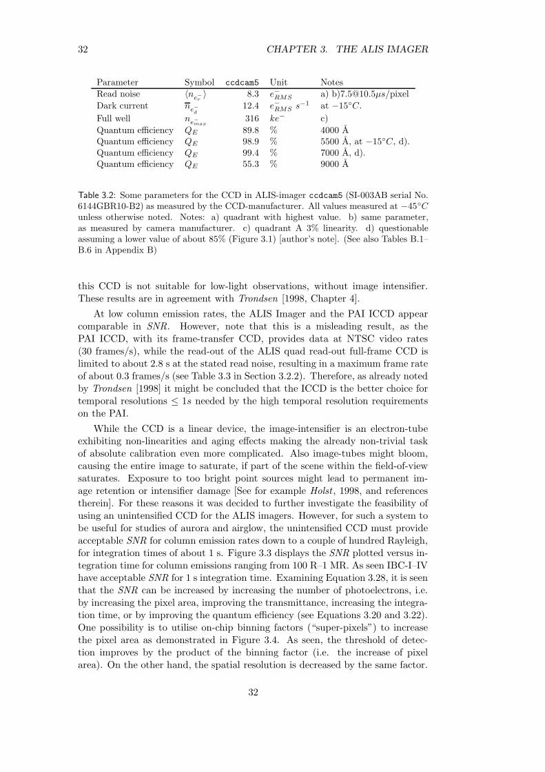
32 CHAPTER 3. THE ALIS IMAGER
Parameter Symbol ccdcam5 Unit Notes
Read noise 〈ne−
r〉 8.3 e−RMS a) b)[email protected]µs/pixel
Dark current ne−
d12.4 e−RMS s−1 at −15C.
Full well ne−
max316 ke− c)
Quantum efficiency QE 89.8 % 4000 AQuantum efficiency QE 98.9 % 5500 A, at −15C, d).Quantum efficiency QE 99.4 % 7000 A, d).Quantum efficiency QE 55.3 % 9000 A
Table 3.2: Some parameters for the CCD in ALIS-imager ccdcam5 (SI-003AB serial No.6144GBR10-B2) as measured by the CCD-manufacturer. All values measured at −45Cunless otherwise noted. Notes: a) quadrant with highest value. b) same parameter,as measured by camera manufacturer. c) quadrant A 3% linearity. d) questionableassuming a lower value of about 85% (Figure 3.1) [author’s note]. (See also Tables B.1–B.6 in Appendix B)
this CCD is not suitable for low-light observations, without image intensifier.These results are in agreement with Trondsen [1998, Chapter 4].
At low column emission rates, the ALIS Imager and the PAI ICCD appearcomparable in SNR. However, note that this is a misleading result, as thePAI ICCD, with its frame-transfer CCD, provides data at NTSC video rates(30 frames/s), while the read-out of the ALIS quad read-out full-frame CCD islimited to about 2.8 s at the stated read noise, resulting in a maximum frame rateof about 0.3 frames/s (see Table 3.3 in Section 3.2.2). Therefore, as already notedby Trondsen [1998] it might be concluded that the ICCD is the better choice fortemporal resolutions ≤ 1s needed by the high temporal resolution requirementson the PAI.
While the CCD is a linear device, the image-intensifier is an electron-tubeexhibiting non-linearities and aging effects making the already non-trivial taskof absolute calibration even more complicated. Also image-tubes might bloom,causing the entire image to saturate, if part of the scene within the field-of-viewsaturates. Exposure to too bright point sources might lead to permanent im-age retention or intensifier damage [See for example Holst , 1998, and referencestherein]. For these reasons it was decided to further investigate the feasibility ofusing an unintensified CCD for the ALIS imagers. However, for such a system tobe useful for studies of aurora and airglow, the unintensified CCD must provideacceptable SNR for column emission rates down to a couple of hundred Rayleigh,for integration times of about 1 s. Figure 3.3 displays the SNR plotted versus in-tegration time for column emissions ranging from 100 R–1 MR. As seen IBC-I–IVhave acceptable SNR for 1 s integration time. Examining Equation 3.28, it is seenthat the SNR can be increased by increasing the number of photoelectrons, i.e.by increasing the pixel area, improving the transmittance, increasing the integra-tion time, or by improving the quantum efficiency (see Equations 3.20 and 3.22).One possibility is to utilise on-chip binning factors (“super-pixels”) to increasethe pixel area as demonstrated in Figure 3.4. As seen, the threshold of detec-tion improves by the product of the binning factor (i.e. the increase of pixelarea). On the other hand, the spatial resolution is decreased by the same factor.
32
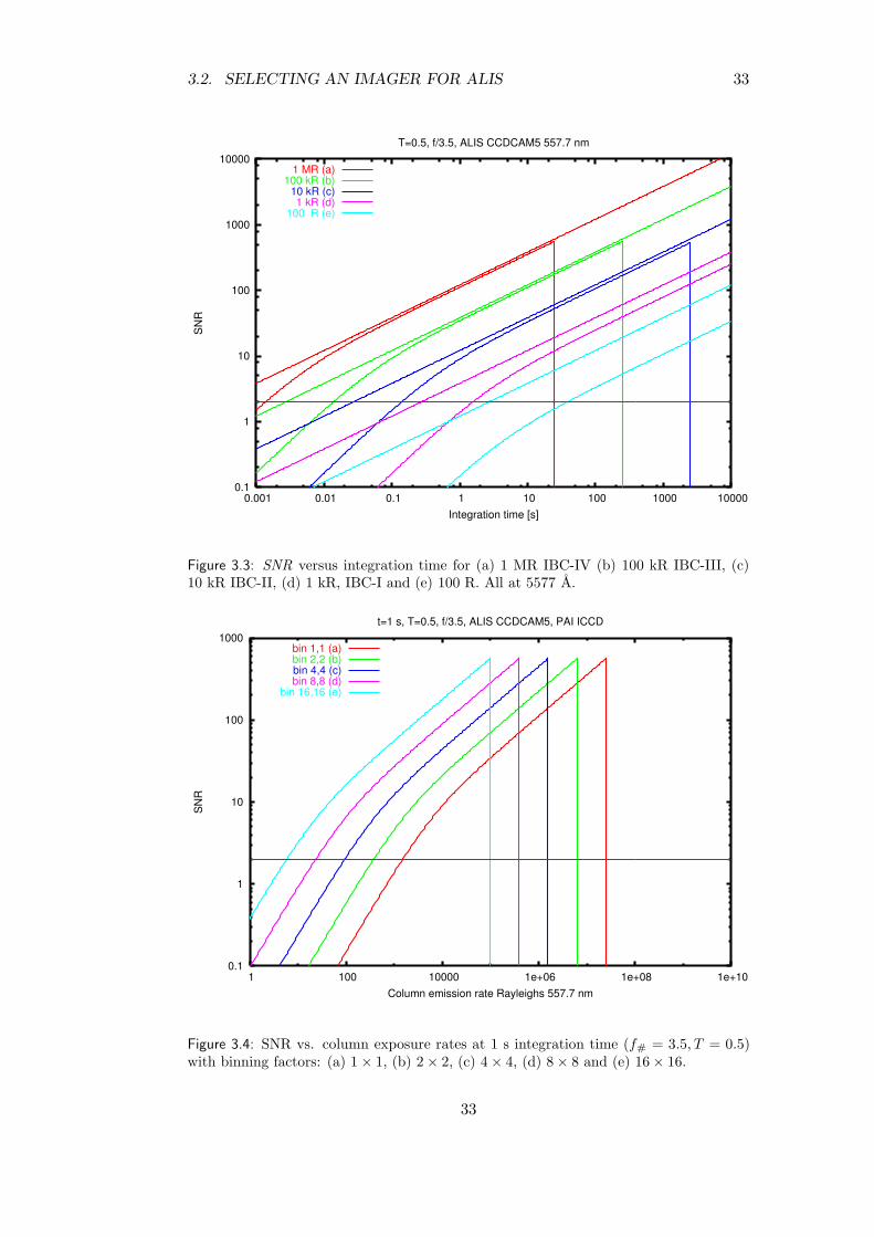
3.2. SELECTING AN IMAGER FOR ALIS 33
0.1
1
10
100
1000
10000
0.001 0.01 0.1 1 10 100 1000 10000
SN
R
Integration time [s]
T=0.5, f/3.5, ALIS CCDCAM5 557.7 nm
1 MR (a) 100 kR (b) 10 kR (c) 1 kR (d)
100 R (e)
Figure 3.3: SNR versus integration time for (a) 1 MR IBC-IV (b) 100 kR IBC-III, (c)10 kR IBC-II, (d) 1 kR, IBC-I and (e) 100 R. All at 5577 A.
0.1
1
10
100
1000
1 100 10000 1e+06 1e+08 1e+10
SN
R
Column emission rate Rayleighs 557.7 nm
t=1 s, T=0.5, f/3.5, ALIS CCDCAM5, PAI ICCD
bin 1,1 (a)bin 2,2 (b)bin 4,4 (c)bin 8,8 (d)
bin 16,16 (e)
Figure 3.4: SNR vs. column exposure rates at 1 s integration time (f# = 3.5, T = 0.5)with binning factors: (a) 1 × 1, (b) 2 × 2, (c) 4 × 4, (d) 8 × 8 and (e) 16× 16.
33
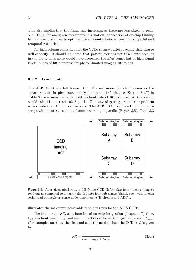
34 CHAPTER 3. THE ALIS IMAGER
This also implies that the frame-rate increases, as there are less pixels to read-out. Thus, for any given measurement situation, application of on-chip binningfactors provides a way to optimise a compromise between sensitivity, spatial andtemporal resolution.
For high column emission rates the CCDs saturate after reaching their chargewell-capacity. It should be noted that pattern noise is not taken into accountin the plots. This noise would have decreased the SNR somewhat at high-signallevels, but is of little interest for photon-limited imaging situations.
3.2.2 Frame rate
The ALIS CCD is a full frame CCD. The read-noise (which increases as thesquare-root of the pixel-rate, mainly due to the 1/f-noise, see Section 3.1.7) inTable 3.2 was measured at a pixel read-out rate of 10.5µs/pixel. At this rate itwould take 11 s to read 10242 pixels. One way of getting around this problemis to divide the CCD into sub-arrays. The ALIS CCD is divided into four sub-arrays with identical read-out channels working in parallel (Figure 3.5). Table 3.3
SubarrayA
CSubarray Subarray
D
BSubarray
Serial readout register Serial readout register
Serial readout registerSerial readout register
Serial readout register
CCDimaging
area
Figure 3.5: At a given pixel rate, a full frame CCD (left) takes four times as long toread-out as compared to an array divided into four sub-arrays (right), each with its ownserial read-out register, sense node, amplifiers, S/H circuits and ADC:s.
illustrates the maximum achievable read-out rates for the ALIS CCDs.
The frame rate, FR, as a function of on-chip integration (“exposure”) time,tint , read-out time, tread , and misc. time before the next image can be read, tmisc,(for example caused by the electronics, or the need to flush the CCD etc.) is givenby:
FR =1
tint + tread + tmisc
(3.43)
34

3.3. THE CCD IMAGER FOR ALIS 35
3.3 The CCD imager for ALIS
Based on the discussion in the previous sections, it might be concluded thatan ICCD imager is better for video-rate observations, mainly due to the longread-out time of a full-frame CCD. On the other hand, the large dynamic range,linearity and long time stability of a scientific-grade unintensified CCD make itan interesting choice for absolute spectroscopic imaging measurements of columnemission rates down to about 1 s time resolution. Therefore it was decided to se-lect a thinned back-side illuminated quad-read-out CCD for the ALIS imagers. Atthe time of specification no commercially available imager met the requirementsof temporal resolution. One company was willing to modify their dual-read-outCCD camera head to a quad-read-out system, resulting in the imager systemfinally procured for ALIS. This section presents a short summary of some of themost important technical details of the six imagers. For further technical inform-ation about the imager hardware, etc., see Preston [1993, 1995]; AstroMed Ltd.[1993] and AstroCam Ltd. [1995]
3.3.1 The camera head
The CCD camera head (CCH) is of dimensions 125×140×144 mm3 (Figure 3.6).A slightly larger front plate (155× 170 mm2) enables mounting the camera head
Figure 3.6: The six ALIS imagers. In the right forefront a sideview of an imager is shown.The front lens, telecentric part with filter wheel, and camera lens connected to the CCDcamera head are seen. The white box on the left is a camera control unit.
to the structure supporting the camera head, optics and filter-wheel. Centred onthe front plate is the optical interface, which consists of a removable ring witha Canon lens-mount. By replacing the ring, the lens-mount can be reconfiguredto a Nikon lens-mount. Thus it is possible to attach a wide variety of stand-ard objective lenses. The thinned back-side illuminated quad-read-out CCD ismounted onto a Peltier cooler inside a hermetically sealed compartment filledwith an inert gas under low-pressure. Light enters through the front-plate hole, amechanical shutter, and a high-quality optical window onto the CCD inside the
35
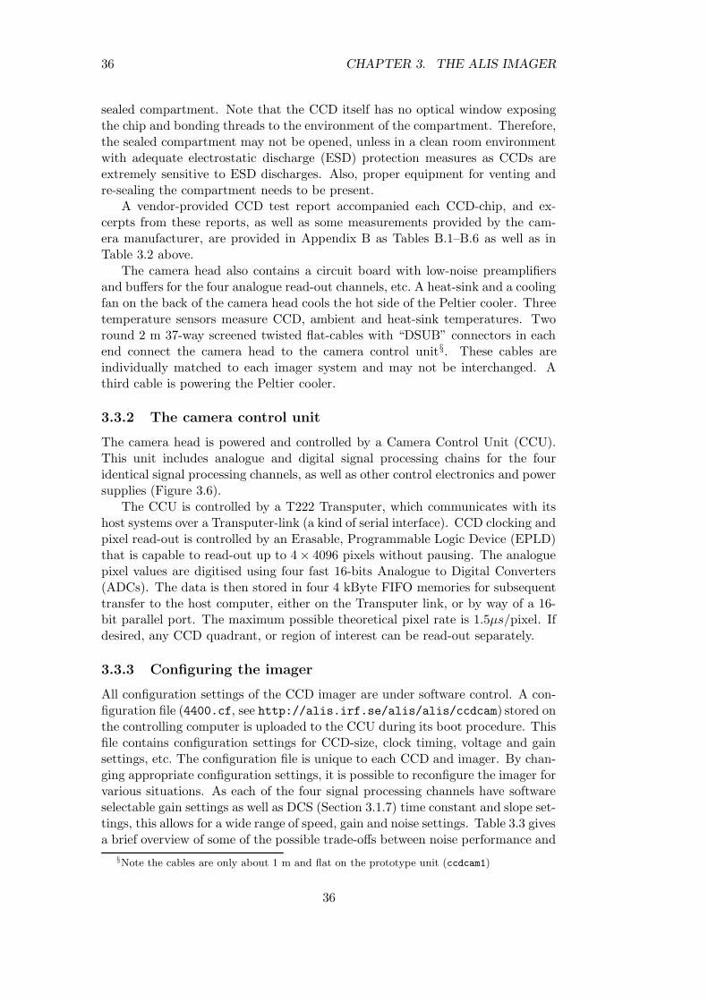
36 CHAPTER 3. THE ALIS IMAGER
sealed compartment. Note that the CCD itself has no optical window exposingthe chip and bonding threads to the environment of the compartment. Therefore,the sealed compartment may not be opened, unless in a clean room environmentwith adequate electrostatic discharge (ESD) protection measures as CCDs areextremely sensitive to ESD discharges. Also, proper equipment for venting andre-sealing the compartment needs to be present.
A vendor-provided CCD test report accompanied each CCD-chip, and ex-cerpts from these reports, as well as some measurements provided by the cam-era manufacturer, are provided in Appendix B as Tables B.1–B.6 as well as inTable 3.2 above.
The camera head also contains a circuit board with low-noise preamplifiersand buffers for the four analogue read-out channels, etc. A heat-sink and a coolingfan on the back of the camera head cools the hot side of the Peltier cooler. Threetemperature sensors measure CCD, ambient and heat-sink temperatures. Tworound 2 m 37-way screened twisted flat-cables with “DSUB” connectors in eachend connect the camera head to the camera control unit§. These cables areindividually matched to each imager system and may not be interchanged. Athird cable is powering the Peltier cooler.
3.3.2 The camera control unit
The camera head is powered and controlled by a Camera Control Unit (CCU).This unit includes analogue and digital signal processing chains for the fouridentical signal processing channels, as well as other control electronics and powersupplies (Figure 3.6).
The CCU is controlled by a T222 Transputer, which communicates with itshost systems over a Transputer-link (a kind of serial interface). CCD clocking andpixel read-out is controlled by an Erasable, Programmable Logic Device (EPLD)that is capable to read-out up to 4 × 4096 pixels without pausing. The analoguepixel values are digitised using four fast 16-bits Analogue to Digital Converters(ADCs). The data is then stored in four 4 kByte FIFO memories for subsequenttransfer to the host computer, either on the Transputer link, or by way of a 16-bit parallel port. The maximum possible theoretical pixel rate is 1.5µs/pixel. Ifdesired, any CCD quadrant, or region of interest can be read-out separately.
3.3.3 Configuring the imager
All configuration settings of the CCD imager are under software control. A con-figuration file (4400.cf, see http://alis.irf.se/alis/alis/ccdcam) stored onthe controlling computer is uploaded to the CCU during its boot procedure. Thisfile contains configuration settings for CCD-size, clock timing, voltage and gainsettings, etc. The configuration file is unique to each CCD and imager. By chan-ging appropriate configuration settings, it is possible to reconfigure the imager forvarious situations. As each of the four signal processing channels have softwareselectable gain settings as well as DCS (Section 3.1.7) time constant and slope set-tings, this allows for a wide range of speed, gain and noise settings. Table 3.3 givesa brief overview of some of the possible trade-offs between noise performance and
§Note the cables are only about 1 m and flat on the prototype unit (ccdcam1)
36

3.3. THE CCD IMAGER FOR ALIS 37
ccdcam pixels µspixel
ne−
r[e−RMS ] tread [s] Notes
1 1124× 1024 6 12–14 1.7 a)1 1124× 1024 8 9–12 2.3 a)1 1124× 1024 13 8–9 3.7 a) default1 1124× 1024 23 7 6.62 1124× 1024 1.6 28 0.52 1124× 1024 2.5 11 0.72 1124× 1024 4.1 10 1.22 1124× 1024 10.5 8 3.0 default3 1124× 1024 1.6 25 0.53 1124× 1024 2.5 13 0.73 1124× 1024 4.1 10 1.23 1124× 1024 7.0 9 2.0 default4 1124× 1024 1.6 25 0.5 b)4 1124× 1024 3.8 13 1.1 b)4 1124× 1024 6.7 10 1.9 b)4 1124× 1024 12.5 9 3.6 b) default5 1056× 1024 1.6 28 0.45 1056× 1024 2.5 11 0.75 1056× 1024 4.1 10 1.15 1056× 1024 10.5 8 2.8 default6 1076× 1024 1.6 25 0.46 1076× 1024 3.8 13 1.06 1076× 1024 6.7 10 1.86 1076× 1024 12.5 9 3.4 default
Table 3.3: CCD-read noise at various pixel clocks for the six ALIS imagers. The valuesare from the vendor-provided configuration files for the imagers.
37

38 CHAPTER 3. THE ALIS IMAGER
read-out speed. For a more detailed understanding of these configuration possib-ilities, please refer to the imager documentation and configuration files. See alsoTable 3.2, Equations 4.7 and 4.8 in Section 4.2.1.
3.3.4 The user port
“Okay, Houston, we’ve had a problem here.” John Leonard Swigert, Jr.
As the T222 Transputer links are capable of no more than 20 Mbits/s, image-data transfer at maximum pixel-clocking would be too slow. To remedy this thecamera controllers are equipped with a 16-bit parallel interface. Originally itwas intended that data from this interface would be read directly by the NIPU,however, due to the fast technical development, an extra computer responsiblefor receiving and storing the image data took over the role of the NIPU (see alsoSection 2.2.2). A prototype fast read-out interface card for a PC computer wasbuilt and tested. During these tests it was found that the user port omitted the50 last pixels of each line on each of the four read-out channels (corresponding toa total of 102400 pixels in the centre 100 columns of the image) thus rendering theimage data useless. Contacts were taken with the camera manufacturer to remedythis. This resulted in a new version of the camera controller software, fixing someof these problems, but now severe intermittent problems arose. Great effort wasmade to find the cause of these data-losses but without success. A solution tothese problems still remains to be found, and meanwhile, the fast read-out modehad to be abandoned.
3.3.5 Operational remarks
At the time of writing, the ALIS imagers have been in operation for up to tenyears. During this time they have produced a large number of images resultingin scientific findings as reported in Chapter 6, and references therein. The maintechnical obstacle has been poor frame-rate as discussed above.
The oldest, prototype imager, (ccdcam1) still works well, as does the newestimager (ccdcam6). The second camera (ccdcam2) developed a problem with iceon the CCD in 1999, probably due to a breach in the hermetic compartment.This problem should be fairly easy to resolve. The remaining cameras havehad intermittent reliability problems related to the electronics. The occurrenceof these problems has increased during the last couple of years. Another issueis that much of the camera electronics is becoming obsolete, severely affectingspare-parts availability. On a short time-scale (3–5 years), a limited maintenanceoperation will most likely bring 4–6 imagers back into operation. However, in alonger perspective, the now rather old imager electronics need to be completelyreplaced. During such a renovation it must be investigated if the most expensivepart of the system (i.e. CCDs), and even the camera heads can be reused. All sixCCD detectors are in good condition, and still among the best imaging detectorsavailable for the scientific objectives of ALIS.
38
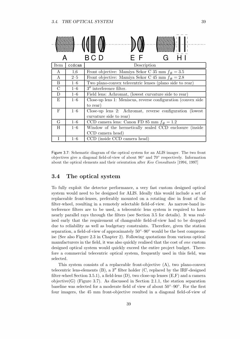
3.4. THE OPTICAL SYSTEM 39
A C D E F G H IBItem ccdcam Description
A 1,6 Front objective: Mamiya Sekor C 35 mm f# = 3.5
A 2–5 Front objective: Mamiya Sekor C 45 mm f# = 2.8
B 1–6 Two plano-convex telecentric lenses (plano side to rear)
C 1–6 3′′ interference filter.
D 1–6 Field lens: Achromat, (lowest curvature side to rear)
E 1–6 Close-up lens 1: Meniscus, reverse configuration (convex sideto rear)
F 1–6 Close-up lens 2: Achromat, reverse configuration (lowestcurvature side to rear)
G 1–6 CCD camera lens: Canon FD 85 mm f# = 1.2
H 1–6 Window of the hermetically sealed CCD enclosure (insideCCD camera head)
I 1–6 CCD (inside CCD camera head)
Figure 3.7: Schematic diagram of the optical system for an ALIS imager. The two frontobjectives give a diagonal field-of-view of about 90 and 70 respectively. Informationabout the optical elements and their orientation after Keo Consultants [1994, 1997]
3.4 The optical system
To fully exploit the detector performance, a very fast custom designed opticalsystem would need to be designed for ALIS. Ideally this would include a set ofreplaceable front-lenses, preferably mounted on a rotating disc in front of thefilter-wheel, resulting in a remotely selectable field-of-view. As narrow-band in-terference filters are to be used, a telecentric lens system is required to havenearly parallel rays through the filters (see Section 3.5 for details). It was real-ised early that the requirement of changeable field-of-view had to be droppeddue to reliability as well as budgetary constraints. Therefore, given the stationseparation, a field-of-view of approximately 50–90 would be the best comprom-ise (See also Figure 2.3 in Chapter 2). Following quotations from various opticalmanufacturers in the field, it was also quickly realised that the cost of one customdesigned optical system would quickly exceed the entire project budget. There-fore a commercial telecentric optical system, frequently used in this field, wasselected.
This system consists of a replaceable front-objective (A), two plano-convextelecentric lens-elements (B), a 3′′ filter holder (C, replaced by the IRF-designedfilter-wheel Section 3.5.1), a field-lens (D), two close-up lenses (E,F) and a cameraobjective(G) (Figure 3.7). As discussed in Section 2.1.1, the station separationbaseline was selected for a moderate field of view of about 50–90. For the firstfour imagers, the 45 mm front-objective resulted in a diagonal field-of-view of
39

40 CHAPTER 3. THE ALIS IMAGER
about 50. Experiences gained from tomographic reconstruction using imagesfrom these four systems resulted in a decision to slightly widen the field-of-viewfor the next two imagers. Consequently these were equipped with a 35 mm front-objective, giving a diagonal field-of-view of about 90.
According to vendor specifications [Keo Consultants, 1994, 1997], the f-num-ber setting on the front lens, f#fl, will determine image brightness on the CCD,as well as the maximum ray-angle through the filter, θmax, given by the followingapproximate formula:
θmax = arctan
(
1
2f#fl
)
(3.44)
A photograph of the six ALIS imagers appears in Figure 3.6.
3.5 Interference filters
To make spectroscopic imaging, narrow-band interference filters are required.These filters are sometimes referred to as Fabry-Perot filters, as they are multiplecavity solid Fabry-Perot etalons [See for example Macleod , 1986; Hernandez ,1986, and references therein]. Rays passing through an interference filter mustbe nearly normal to the filter system. This dictates the use of a telecentric lens-system as discussed in Section 3.4.
The passband of an interference filter with effective index of refraction, Ne,(Ne ≈ 2 for most interference filters) and filter centre wavelength at normalincidence, λcw, shifts to λθ at angle of incidence θ according to the followingequation¶:
λθ = λcw
√
1 − sin2 θ
N2e
(3.45)
As seen, the passband shifts to shorter wavelengths at increasing angle of incid-ence. This fact is often utilised to fine-tune filters, or to measure backgroundintensity by tilting the filter out of the passband for the emission line understudy. In the case of the ALIS optics, let θ define a cone between normal in-cidence and θmax given by Equation 3.44. Optimum filters for this situationshould be designed as insensitive to angle as possible, and the bandwidth shouldbe wide enough to pass the wavelength(s) of interest at all angles within thecone. Thus θmax also defines the minimum possible bandwidth of the filter.Given a wavelength region of interest, specification of the optical system, fil-ter centre wavelength (λcw) and desired filter-bandwidth, ∆λ, an optimal filteris manufactured. As almost every batch of filters are tailored for a particularapplication, high-quality interference filters for imaging applications are ratherexpensive devices. Data on the filters used for ALIS appear in Tables 3.4-3.5.A discussion of the selected emission lines is found in the work by Gustavsson[2000, Chapter 2] and references therein.
¶from the filter manufacturer (http://www.barrassociates.com/terms.php?type=angle),see also [Jones, 1974]
40
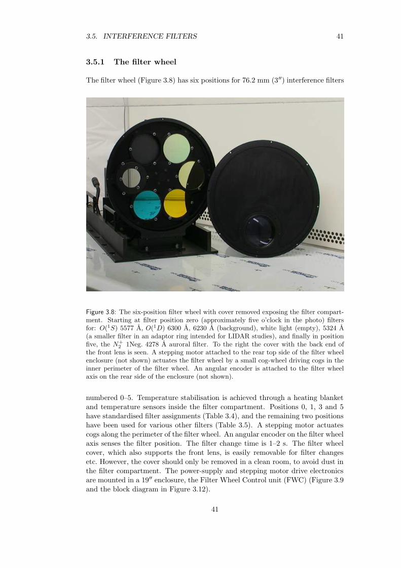
3.5. INTERFERENCE FILTERS 41
3.5.1 The filter wheel
The filter wheel (Figure 3.8) has six positions for 76.2 mm (3′′) interference filters
Figure 3.8: The six-position filter wheel with cover removed exposing the filter compart-ment. Starting at filter position zero (approximately five o’clock in the photo) filtersfor: O(1S) 5577 A, O(1D) 6300 A, 6230 A (background), white light (empty), 5324 A(a smaller filter in an adaptor ring intended for LIDAR studies), and finally in positionfive, the N+
2 1Neg. 4278 A auroral filter. To the right the cover with the back end ofthe front lens is seen. A stepping motor attached to the rear top side of the filter wheelenclosure (not shown) actuates the filter wheel by a small cog-wheel driving cogs in theinner perimeter of the filter wheel. An angular encoder is attached to the filter wheelaxis on the rear side of the enclosure (not shown).
numbered 0–5. Temperature stabilisation is achieved through a heating blanketand temperature sensors inside the filter compartment. Positions 0, 1, 3 and 5have standardised filter assignments (Table 3.4), and the remaining two positionshave been used for various other filters (Table 3.5). A stepping motor actuatescogs along the perimeter of the filter wheel. An angular encoder on the filter wheelaxis senses the filter position. The filter change time is 1–2 s. The filter wheelcover, which also supports the front lens, is easily removable for filter changesetc. However, the cover should only be removed in a clean room, to avoid dust inthe filter compartment. The power-supply and stepping motor drive electronicsare mounted in a 19′′ enclosure, the Filter Wheel Control unit (FWC) (Figure 3.9and the block diagram in Figure 3.12).
41
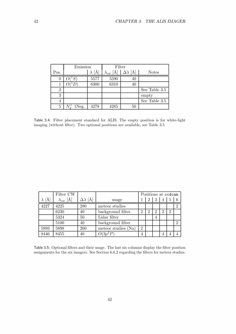
42 CHAPTER 3. THE ALIS IMAGER
Emission FilterPos. λ [A] λcw [A] ∆λ [A] Notes
0 O(1S) 5577 5590 40
1 O(1D) 6300 6310 40
2 See Table 3.5
3 empty
4 See Table 3.5
5 N+2 1Neg. 4278 4285 50
Table 3.4: Filter placement standard for ALIS. The empty position is for white-lightimaging (without filter). Two optional positions are available, see Table 3.5
Filter CW Positions at ccdcamλ [A] λcw [A] ∆λ [A] usage 1 2 3 4 5 6
4227 4225 280 meteor studies 2
6230 40 background filter. 2 2 2 2 2
5324 50 Lidar filter 4
5100 40 background filter. 2
5893 5898 200 meteor studies (Na) 2
8446 8455 40 O(3p3P ) 4 4 4 4
Table 3.5: Optional filters and their usage. The last six columns display the filter positionassignments for the six imagers. See Section 6.6.2 regarding the filters for meteor studies.
42
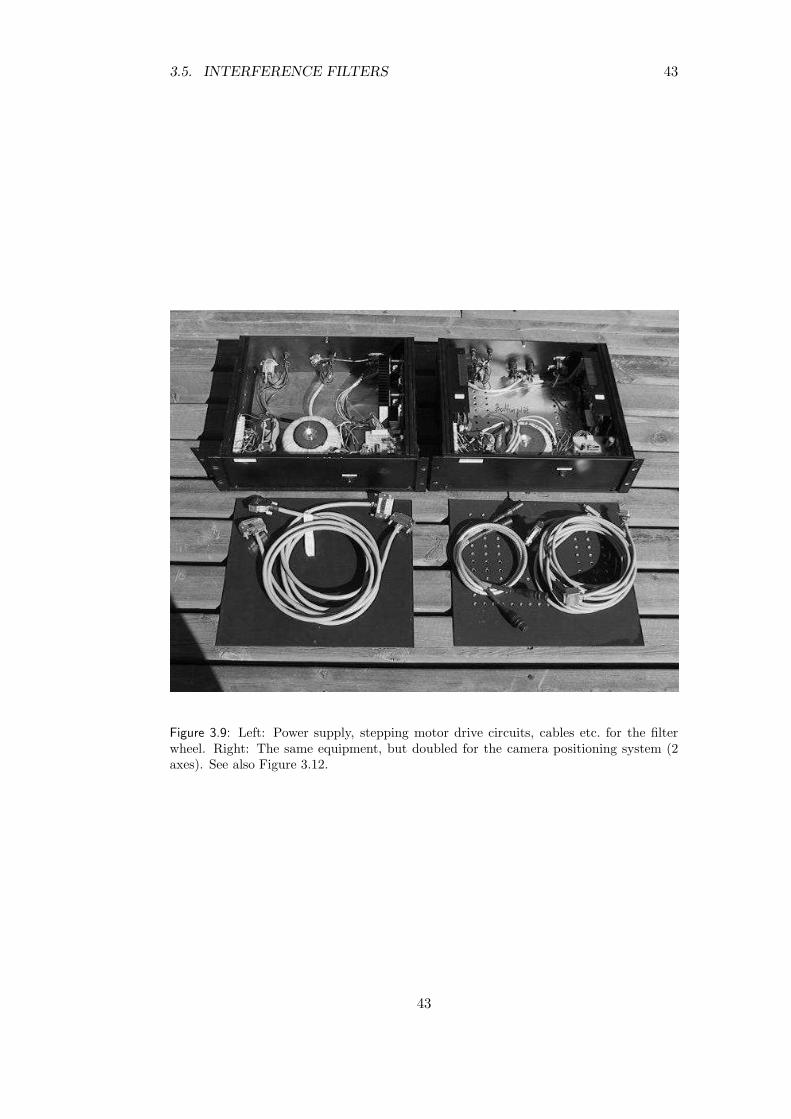
3.5. INTERFERENCE FILTERS 43
Figure 3.9: Left: Power supply, stepping motor drive circuits, cables etc. for the filterwheel. Right: The same equipment, but doubled for the camera positioning system (2axes). See also Figure 3.12.
43

44 CHAPTER 3. THE ALIS IMAGER
3.6 The camera positioning system
As the imagers are using moderate fields-of-view (Figure 2.3), a Camera Position-ing System (CPS) is required in order to be able to configure ALIS for variousimaging situations. For example, when running in a tomographic mode, observa-tion of a common volume centred on an auroral arc is desired, while maximumsky coverage, or tracking of the foot-point of a spacecraft might be the objectiveof other observational modes. When observing for example HF-pump enhancedairglow (Section 6.4), the cameras need to point towards the anticipated regionof enhanced airglow above the EISCAT-Heating facility in Tromsø
Initially a traditional azimuth/elevation drive with rotation in azimuth andelevation was considered, but it was found that such a drive would be difficultand expensive to build given the size and weight of the imager and the availablespace at the station. There is also a cable wrap problem associated with theazimuth drive, where the drive would have to rotate back 360 in certain imagingsituations. Because of this, a solution consisting of three frames mounted insideone another was selected.
The two innermost frames are mounted on perpendicular axes. The ALISimager is attached to the innermost frame (Figure 3.10). Stepping motors areconnected to one end of each axis via a worm-gear assembly, and an angularencoder is attached to the other end. The worm-gear assembly gives an automaticbrake when the stepping motors are disengaged, but also introduces a small lag.The innermost axis is denoted α and the outer axis β. In this way it is possibleto reach any region on the sky, keeping the image rotations small and withoutwrapping the cables. Also the cable lengths can be kept short (about 0.5 m ) andthe imager is accessible for maintenance and fairly easy to remove. A worst-caserepositioning typically takes less than 10 s, and the accuracy is 0.01 as long asthe stepping motors are engaged.
The CPS Control unit (CPC) is a similar electronics unit to the FWC (Fig-ure 3.9) and contains the power supply and electronics for the CPS. Both theFWC and the CPC are in turn controlled by the NIPU (Section 2.2.2). Conver-sion of set azimuth, aφ, and zenith-angle, zθ, of the optical axis, into α and βvalues is automatically done by the NIPU software according to these equations:
α = arctan(sin aφ tan zθ) (3.46)
β = − arcsin(cos aφ sin zθ) (3.47)
Azimuth is defined as zero towards North and 90 towards east. Zenith angle iszero in zenith and increases towards the horizon, (i.e. zθ = 90 − hθ, where hθ isthe elevation). It is worth remembering that the azimuth value is undefined forsmall zenith angles. The maximum zenith angle is typically about 54.
To simplify the use of ALIS, a set of standard pre-programmed positions forvarious typical observing requirements are available (Table 3.6 and Figure 3.11).
The present CPS has been in use since 1993. Since being put into operationthe CPS appears to be reliable and it has worked for years without any majorproblems. Worm-gear adjustment due to mechanical wear, as well as some angu-lar encoder failures, probably due to an aging laser-diode in the angular encoder,
44
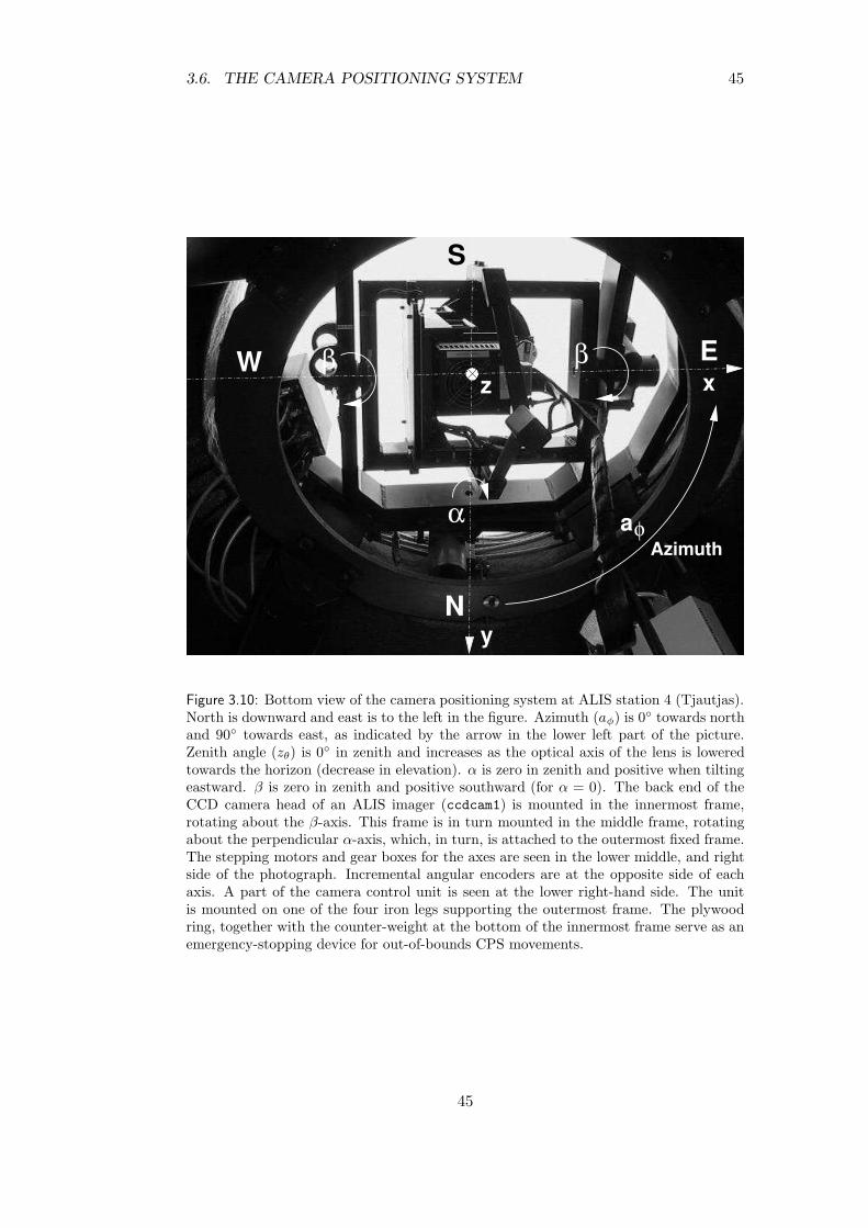
3.6. THE CAMERA POSITIONING SYSTEM 45
aφ
Azimuth
W E
S
α
x
Ny
zβ β
Figure 3.10: Bottom view of the camera positioning system at ALIS station 4 (Tjautjas).North is downward and east is to the left in the figure. Azimuth (aφ) is 0 towards northand 90 towards east, as indicated by the arrow in the lower left part of the picture.Zenith angle (zθ) is 0 in zenith and increases as the optical axis of the lens is loweredtowards the horizon (decrease in elevation). α is zero in zenith and positive when tiltingeastward. β is zero in zenith and positive southward (for α = 0). The back end of theCCD camera head of an ALIS imager (ccdcam1) is mounted in the innermost frame,rotating about the β-axis. This frame is in turn mounted in the middle frame, rotatingabout the perpendicular α-axis, which, in turn, is attached to the outermost fixed frame.The stepping motors and gear boxes for the axes are seen in the lower middle, and rightside of the photograph. Incremental angular encoders are at the opposite side of eachaxis. A part of the camera control unit is seen at the lower right-hand side. The unitis mounted on one of the four iron legs supporting the outermost frame. The plywoodring, together with the counter-weight at the bottom of the innermost frame serve as anemergency-stopping device for out-of-bounds CPS movements.
45
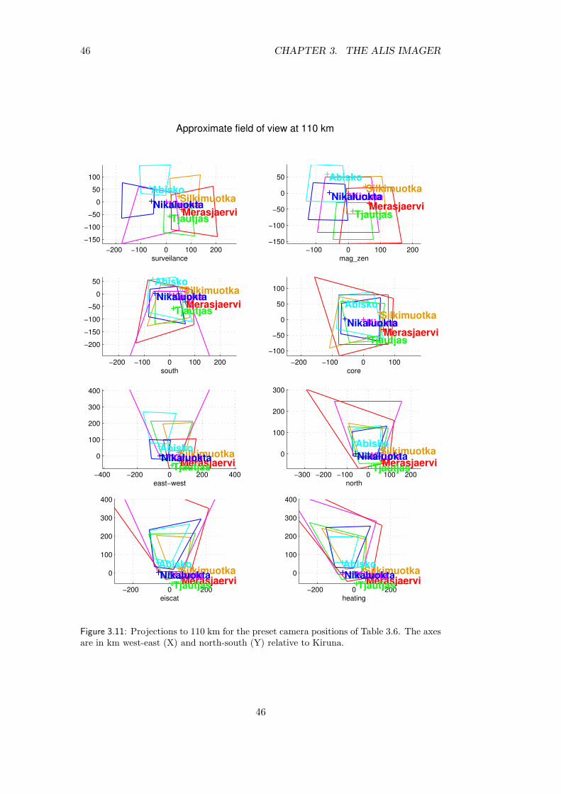
46 CHAPTER 3. THE ALIS IMAGER
−200 −100 0 100 200−150
−100
−50
0
50
100
MerasjaerviSilkimuotka
Tjautjas
surveilance
KirunaNikaluoktaAbisko
−100 0 100 200−150
−100
−50
0
50
Merasjaervi
Silkimuotka
Tjautjas
mag_zen
KirunaNikaluokta
Abisko
−200 −100 0 100 200
−200
−150
−100
−50
0
50
MerasjaerviSilkimuotka
TjautjasKiruna
south
NikaluoktaAbisko
−200 −100 0 100
−100
−50
0
50
100
Merasjaervi
Silkimuotka
Tjautjas
Kiruna
core
Nikaluokta
Abisko
−400 −200 0 200 400
0
100
200
300
400
MerasjaerviSilkimuotka
TjautjasKiruna
east−west
NikaluoktaAbisko
−300 −200 −100 0 100 200
0
100
200
300
MerasjaerviSilkimuotka
TjautjasKirunaNikaluokta
Abisko
north
−200 0 200
0
100
200
300
400
MerasjaerviSilkimuotka
TjautjasKiruna
eiscat
NikaluoktaAbisko
Approximate field of view at 110 km
−200 0 200
0
100
200
300
400
MerasjaerviSilkimuotka
TjautjasKiruna
heating
NikaluoktaAbisko
Figure 3.11: Projections to 110 km for the preset camera positions of Table 3.6. The axesare in km west-east (X) and north-south (Y) relative to Kiruna.
46

3.7. SUMMARY 47
1 KRN 2 MER 3 SIL 4 TJA 5 ABK 6 NILaφ zθ aφ zθ aφ zθ aφ zθ aφ zθ aφ zθ
core — Centred on a volume above Kiruna0 0 298 24 249 28 346 20 130 24 90 20
eiscat — Optimised for field-aligned EISCAT studies0 39 348 42 350 32 0 42 20 35 15 42
E-W — Optimise east-west field-of-view0 39 0 15 0 32 0 42 0 35 0 15
heating — Optimised for HF-pump enhanced airglow346 37 340 40 330 37 345 44 5 25 5 40
mag-Z — Local magnetic zenith180 12 180 12 180 12 180 12 180 12 180 12
north — Centred on a volume north of Kiruna0 30 330 33 311 25 355 33 85 22 44 26
south — Centred on a volume south of Kiruna180 30 250 23 215 28 260 7 148 31 135 23
surv — Optimised for maximum field-of-view225 20 100 14 45 12 115 15 30 14 270 20
Table 3.6: ALIS preset camera positions. The columns give azimuth and zenith anglesfor the six stations. See also Figure 3.11.
have been encountered so far. Future CPS units will need a slight re-design ofthe hardware and a micro-controller replacing the obsolete NIPU. The existingdevices will need upgraded electronics including new angular encoders as part ofnormal system maintenance.
3.7 Summary
This chapter has discussed the selection and design of the ALIS imager and itsassociated subsystems. In summary these systems consist of the following items:
ALIS imager: consisting of Optics (Section 3.4), filter-wheel (Section 3.5.1),with interference filters (Section 3.5) and the CCD Camera Head (CCH)mounted together as a removable unit. Six ALIS imagers exist to date,and they are denoted ccdcam 1–6 (See Section 3.3.1 and Tables B.1–B.6 inAppendix B. It is important not to confuse these numbers with the stationnumbers (Table 2.3).
Camera Control Unit (CCU) : containing power-supply and electronics forthe camera head. The CCUs are individually adapted for each camera headand must not be used with a different camera head.
Filter-Wheel Control unit (FWC) : containing power-supply and electron-ics for the filter-wheel (Figure 3.9).
Camera Positioning System (CPS) : Supports the ALIS Imager and pro-vides the possibility to remotely point the camera to any desired region ofthe sky. The CPS is attached to the camera-stand (Section 3.6).
47
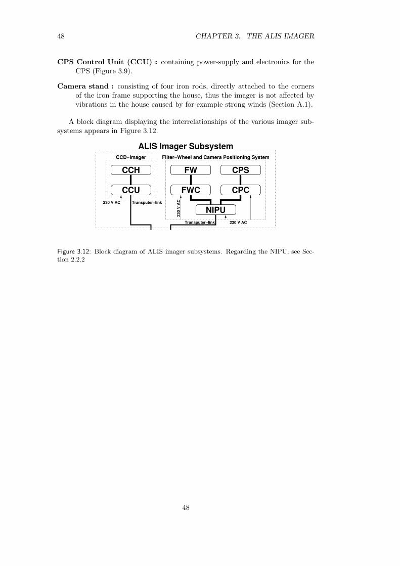
48 CHAPTER 3. THE ALIS IMAGER
CPS Control Unit (CCU) : containing power-supply and electronics for theCPS (Figure 3.9).
Camera stand : consisting of four iron rods, directly attached to the cornersof the iron frame supporting the house, thus the imager is not affected byvibrations in the house caused by for example strong winds (Section A.1).
A block diagram displaying the interrelationships of the various imager sub-systems appears in Figure 3.12.
Transputer−link
CCH
CCU230 V AC
CCD−Imager
FWC
FW CPS
CPC
NIPU
230
V A
C
Filter−Wheel and Camera Positioning System
Transputer−link 230 V AC
ALIS Imager Subsystem
Figure 3.12: Block diagram of ALIS imager subsystems. Regarding the NIPU, see Sec-tion 2.2.2
48
49
Chapter 4
Calibrating ALIS
“Gor vad du kan — och uppgiften skall vila latt i din hand, sa latt att dumed forvantan stracker dig mot det svarare prov som kan folja.
Det ar nar morgonglansen bytts i middagstrotthet, nar benmusklerna skalvavid anspanningen, vagen tycks oandlig och plotsligt ingenting vill ga riktigtsom du onskar — det ar da du inte far tveka.” Dag Hammarskjold
Calibration is the process of answering the following two basic questions:
1. What physical value does the pixel represent?
2. How is each pixel mapped to the observed object?
Answering these two rather simple questions is often no simple task.
In the case of a classical photometer, there is only one detector with a rel-atively narrow field-of-view. For an ALIS imager there are about 106 individualdetectors (pixels) covering a moderate field-of-view (50–60). Calibrating imagedata is therefore a considerably more complex issue compared to calibrating aphotometer.
An ALIS Imager produces two-dimensional images of size m×n pixels. Eachpixel is represented by a signed 16-bit integer value (−32768–32767). This valueis often referred to as digital output, DN ij . The indices are pixel columns, i, andpixel rows, j, These go from the first to the last pixel in each direction (Figure 4.1).Note that the number of pixels in each direction should be divided by the on-chipbinning factors (Section 3.2.1). Supplemental information is contained in theimage header (for example azimuth, zenith-angle, integration time, filter, etc.).
4.1 Removing the instrument signature
First it is necessary to remove the instrument signature from the image data.This task is sometime called “data reduction”. The procedure is to a large extentsimilar to that followed when reducing astronomical CCD image data [for exampleMassey , 1992]. In most cases the reduction is carried out first by removingadditive effects, and then proceeding with multiplicative effects.
49
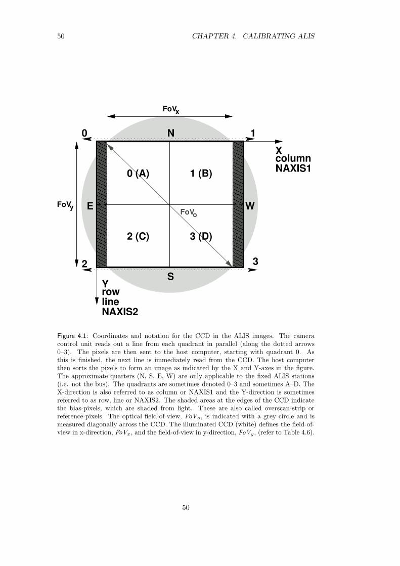
50 CHAPTER 4. CALIBRATING ALIS
FoVx
FoVy
rowY
lineNAXIS2
XcolumnNAXIS1
1 (B)
3 (D)2 (C)
0 (A)
E W
N
S
10
2 3
oFoV
Figure 4.1: Coordinates and notation for the CCD in the ALIS images. The cameracontrol unit reads out a line from each quadrant in parallel (along the dotted arrows0–3). The pixels are then sent to the host computer, starting with quadrant 0. Asthis is finished, the next line is immediately read from the CCD. The host computerthen sorts the pixels to form an image as indicated by the X and Y-axes in the figure.The approximate quarters (N, S, E, W) are only applicable to the fixed ALIS stations(i.e. not the bus). The quadrants are sometimes denoted 0–3 and sometimes A–D. TheX-direction is also referred to as column or NAXIS1 and the Y-direction is sometimesreferred to as row, line or NAXIS2. The shaded areas at the edges of the CCD indicatethe bias-pixels, which are shaded from light. These are also called overscan-strip orreference-pixels. The optical field-of-view, FoVo , is indicated with a grey circle and ismeasured diagonally across the CCD. The illuminated CCD (white) defines the field-of-view in x-direction, FoVx , and the field-of-view in y-direction, FoVy , (refer to Table 4.6).
50
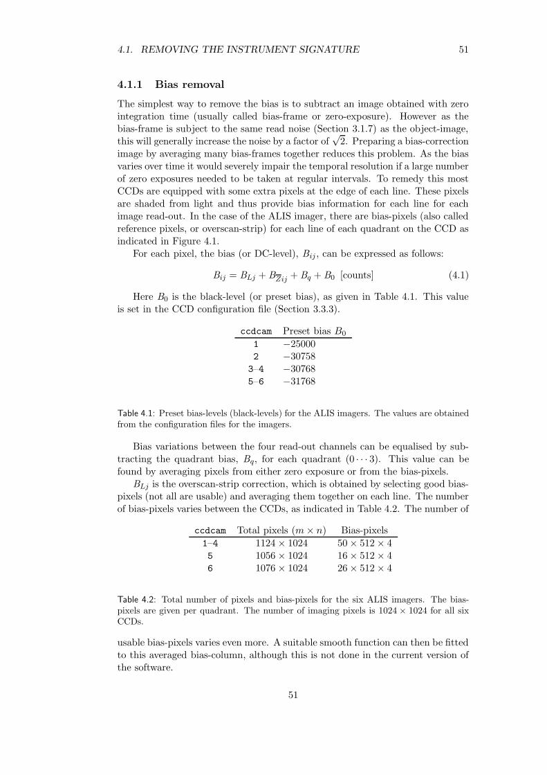
4.1. REMOVING THE INSTRUMENT SIGNATURE 51
4.1.1 Bias removal
The simplest way to remove the bias is to subtract an image obtained with zerointegration time (usually called bias-frame or zero-exposure). However as thebias-frame is subject to the same read noise (Section 3.1.7) as the object-image,this will generally increase the noise by a factor of
√2. Preparing a bias-correction
image by averaging many bias-frames together reduces this problem. As the biasvaries over time it would severely impair the temporal resolution if a large numberof zero exposures needed to be taken at regular intervals. To remedy this mostCCDs are equipped with some extra pixels at the edge of each line. These pixelsare shaded from light and thus provide bias information for each line for eachimage read-out. In the case of the ALIS imager, there are bias-pixels (also calledreference pixels, or overscan-strip) for each line of each quadrant on the CCD asindicated in Figure 4.1.
For each pixel, the bias (or DC-level), Bij , can be expressed as follows:
Bij = BLj + BZij + Bq + B0 [counts] (4.1)
Here B0 is the black-level (or preset bias), as given in Table 4.1. This valueis set in the CCD configuration file (Section 3.3.3).
ccdcam Preset bias B0
1 −250002 −30758
3–4 −307685–6 −31768
Table 4.1: Preset bias-levels (black-levels) for the ALIS imagers. The values are obtainedfrom the configuration files for the imagers.
Bias variations between the four read-out channels can be equalised by sub-tracting the quadrant bias, Bq, for each quadrant (0 · · · 3). This value can befound by averaging pixels from either zero exposure or from the bias-pixels.
BLj is the overscan-strip correction, which is obtained by selecting good bias-pixels (not all are usable) and averaging them together on each line. The numberof bias-pixels varies between the CCDs, as indicated in Table 4.2. The number of
ccdcam Total pixels (m × n) Bias-pixels
1–4 1124 × 1024 50 × 512 × 45 1056 × 1024 16 × 512 × 46 1076 × 1024 26 × 512 × 4
Table 4.2: Total number of pixels and bias-pixels for the six ALIS imagers. The bias-pixels are given per quadrant. The number of imaging pixels is 1024 × 1024 for all sixCCDs.
usable bias-pixels varies even more. A suitable smooth function can then be fittedto this averaged bias-column, although this is not done in the current version ofthe software.
51
52 CHAPTER 4. CALIBRATING ALIS
As mentioned initially, to further enhance the bias removal, it is also possibleto obtain k bias-frames (Typically at least 25 images), resulting in an averagedbias-correction image, BZij .
∀(i, j) : BZij =1
k
k∑
1
(DN Zij − BLj − Bq − B0) [counts] (4.2)
This correction is normally only present when calibrating the imagers.
4.1.2 Dark-current
Correction for the dark-current is performed by taking several dark-exposures,i.e. long exposures (tint ≥ 600 s) with the shutter closed. The dark-currentcorrection image, Dij , is then produced by averaging these images together inmuch the same way as the averaged bias-correction image (Equation 4.2):
∀(i, j) : Dij =1
k
k∑
1
1
tint,k
(
DN Dij − BZij − BLj − Bq − B0
)
[counts] (4.3)
Here tint,k is the integration time for image k.However for the ALIS imagers, this correction has been found to be negli-
gible for integration times less than 10–15 minutes. Therefore, no dark-currentcorrection is made except for very special cases.
4.1.3 Flat-field correction
The purpose of the flat-field calibration is to remove multiplicative variationsintroduced by pixel-to-pixel sensitivity differences, vignetting in the optics, vari-ation in transmittance on the filter surface, etc.. This is done by taking a largenumber of images of a uniform flat-field source:
∀(i, j, λ) : Fijλ =1
k
k∑
1
1
tint,k
(
DN Fijλ − BZij − BLj − Bq − B0 − Dij
)
(4.4)
In this equation Fijλ is the flat-field correction. The index, λ, indicates that theflat-field correction images should be obtained for each wavelength of interest.Normally this means one set of flat-field images per filter. However a calibrationfacility which can take measurements for several wavelengths within the filterpassband would enable measurements of the combined effects of transmittances(Section 3.1.3) and quantum efficiency (Section 3.1.6) for the entire imaging sys-tem (and as a function of wavelength).
The moderate fields-of-view (50–60) for the ALIS imagers necessitate anintegrating sphere of a sufficient diameter for flat-field calibration [i.e. about1.5–2 m, see Brandstrom, 2000; Labsphere, 1997, and references therein.].
Numerous attempts were made to use simpler methods, such as cloudy skies,white screens, diffuse spherical lamp covers etc. to obtain reasonably good flat-field images. None of these attempts provided flat-field images of sufficient qual-ity, as non-uniformities and gradients were hard to avoid with these simple ap-proaches.
52
4.1. REMOVING THE INSTRUMENT SIGNATURE 53
One ALIS imager (ccdcam6) has actually been calibrated in the integratingsphere facility at National Institute of Polar Research, Japan [Okano et al., 1997].The results from this calibration (using white light) are described by Urashimaet al. [1999]. Due to the considerable distance to this facility it would be difficultto perform flat-field calibrations for all cameras, as would be required. Thereforeit is hoped that a similar calibration facility will be established in the proximityof the optical instruments in northern Scandinavia. This was proposed by Steen[1998]. Such a facility would be beneficial to many imaging devices in Europe.
So far no proper flat-field calibration are done on the ALIS images on a regularbasis. Instead, the flat-field correction is solely based on a mathematical model ofthe vignetting in the optical system [Gustavsson, 2000, Chapter 5]. (This modelresembles the “natural vignetting” of cos4 θ discussed in Section 3.1.3). Despitethe fact that this model does not take variations in filter-transmission, pixel-to-pixel sensitivity variations, etc. into account, it has proved to work reasonablywell.
4.1.4 Bad-pixel correction
Defects are unavoidable in the production of a CCD, so defect-free chips areextremely rare and expensive. The CCDs used for the ALIS imagers are ofscientific grade, allowing for only a few pixel-defects. The pixel-defects, and howto detect them, can be summarised as follows [after Holst , 1998]:
Point defect: Pixel with deviation of more than 6 % compared to adjacentpixels when illuminated to 70 % saturation. (Expose a white area to about70 % of the dynamic range.)
Hot point defect: Pixels with extremely high output voltage. Typically a pixelwhose dark-current is 10 times higher than the average dark-current. (Takea zero or dark image.)
Dead pixels: Pixels with low output voltage and/or poor responsitivity. Typ-ically a pixel whose output is one half of the others when the backgroundnearly fills the wells. (Expose a white area.)
Pixel traps: A trap interferes with the charge transfer process and results ineither a partial or whole bad line, either all white or all dark. (Take a zero,dark or object image, depending on type of trap)
Column defect: Many (typically 10 or more) point defects in a single column.May be caused by pixel traps (see above).
Cluster defect: A cluster (grouping) of pixels with point defects (see above).
Although the CCDs in the ALIS imager are of scientific grade, there are a fewpixel-defects present on each CCD. These defects have been identified by manu-ally inspecting the images. The bad pixels are then removed by substitutinginterpolated values from adjacent pixels.
53
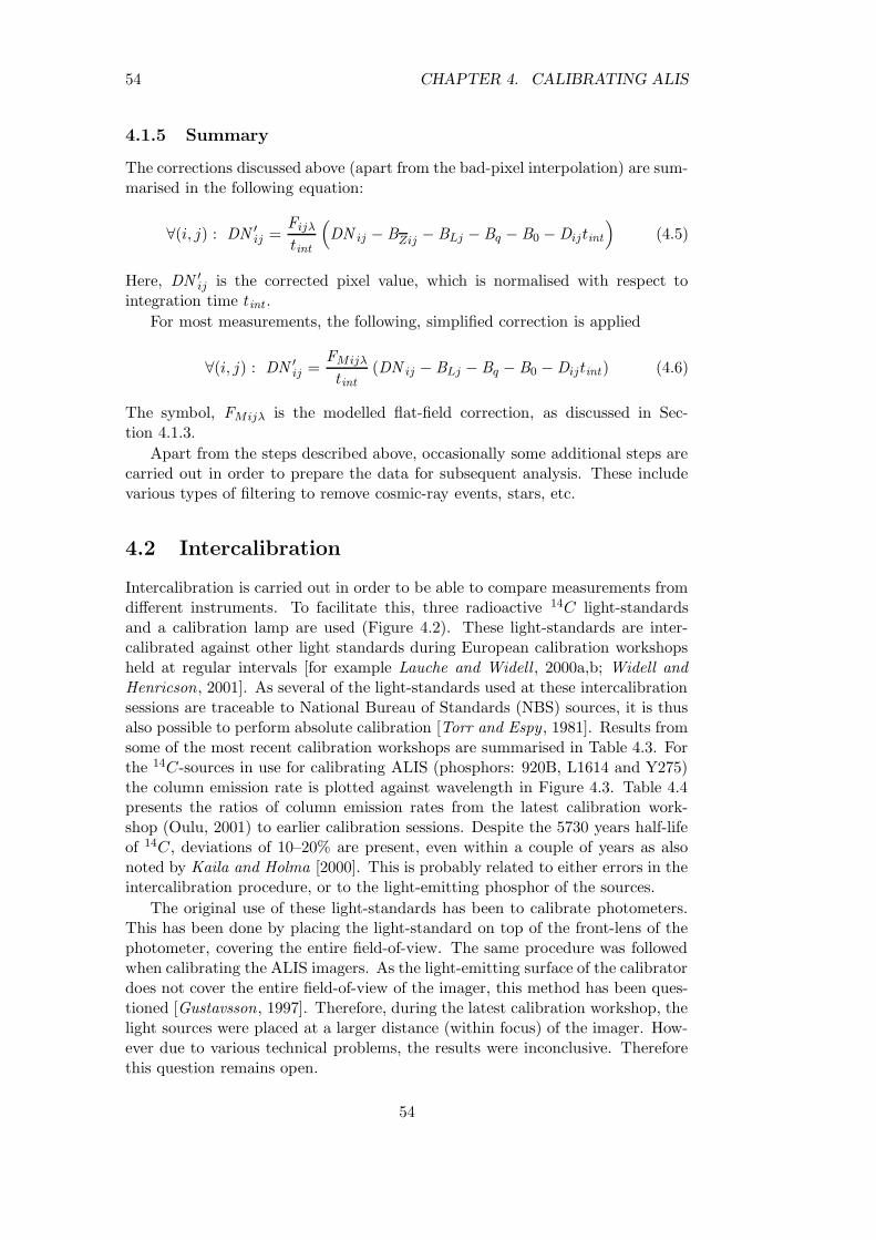
54 CHAPTER 4. CALIBRATING ALIS
4.1.5 Summary
The corrections discussed above (apart from the bad-pixel interpolation) are sum-marised in the following equation:
∀(i, j) : DN ′ij =
Fijλ
tint
(
DN ij − BZij − BLj −Bq − B0 − Dijtint
)
(4.5)
Here, DN ′ij is the corrected pixel value, which is normalised with respect to
integration time tint .
For most measurements, the following, simplified correction is applied
∀(i, j) : DN ′ij =
FMijλ
tint
(DN ij − BLj − Bq − B0 − Dijtint) (4.6)
The symbol, FMijλ is the modelled flat-field correction, as discussed in Sec-tion 4.1.3.
Apart from the steps described above, occasionally some additional steps arecarried out in order to prepare the data for subsequent analysis. These includevarious types of filtering to remove cosmic-ray events, stars, etc.
4.2 Intercalibration
Intercalibration is carried out in order to be able to compare measurements fromdifferent instruments. To facilitate this, three radioactive 14C light-standardsand a calibration lamp are used (Figure 4.2). These light-standards are inter-calibrated against other light standards during European calibration workshopsheld at regular intervals [for example Lauche and Widell , 2000a,b; Widell andHenricson, 2001]. As several of the light-standards used at these intercalibrationsessions are traceable to National Bureau of Standards (NBS) sources, it is thusalso possible to perform absolute calibration [Torr and Espy , 1981]. Results fromsome of the most recent calibration workshops are summarised in Table 4.3. Forthe 14C-sources in use for calibrating ALIS (phosphors: 920B, L1614 and Y275)the column emission rate is plotted against wavelength in Figure 4.3. Table 4.4presents the ratios of column emission rates from the latest calibration work-shop (Oulu, 2001) to earlier calibration sessions. Despite the 5730 years half-lifeof 14C, deviations of 10–20% are present, even within a couple of years as alsonoted by Kaila and Holma [2000]. This is probably related to either errors in theintercalibration procedure, or to the light-emitting phosphor of the sources.
The original use of these light-standards has been to calibrate photometers.This has been done by placing the light-standard on top of the front-lens of thephotometer, covering the entire field-of-view. The same procedure was followedwhen calibrating the ALIS imagers. As the light-emitting surface of the calibratordoes not cover the entire field-of-view of the imager, this method has been ques-tioned [Gustavsson, 1997]. Therefore, during the latest calibration workshop, thelight sources were placed at a larger distance (within focus) of the imager. How-ever due to various technical problems, the results were inconclusive. Thereforethis question remains open.
54
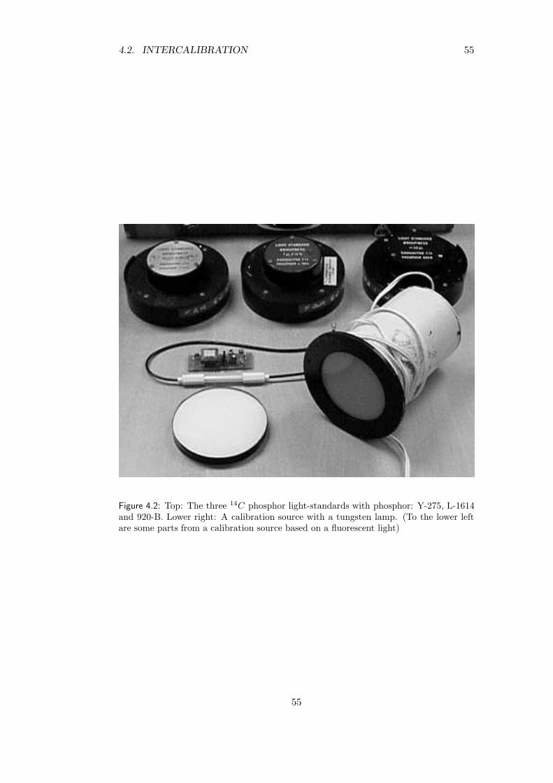
4.2. INTERCALIBRATION 55
Figure 4.2: Top: The three 14C phosphor light-standards with phosphor: Y-275, L-1614and 920-B. Lower right: A calibration source with a tungsten lamp. (To the lower leftare some parts from a calibration source based on a fluorescent light)
55

56 CHAPTER 4. CALIBRATING ALIS
Sources Column emission rate [R/A] at Filter [A]calibration year 3914 4280 4866 5573 5882 6299 6562
Esrange, tungsten lampStockholm 2000 1.3 4.1 30 212 310 532 553Oulu 2001 0.53 1.5 11.6 82 122 233 171IRF, UJO 920BLysebu 1985 5.1 126.0 61.5 18.6 10.5 6.7 8.1Lindau 1999 4.4 102 60 22 12 7.6 2.4Stockholm 2000 4.6 109 64 23 12.7 10 8.5Oulu 2001 5.2 105 65 22 13 9.2 1.2IRF, UJO L1614Lysebu 1985 0.07 0.73 32.5 27.7 8.7 2.5 4.3Lindau 1999 0.6 1 37 33 9.3 1 2Stockholm 2000 0.07 1.0 40 35 9.6 0.36 0.57Oulu 2001 0.1 1.1 38 27 7 1.2 10.2IRF, UJO Y275Lysebu 1985 0.03 0.3 3.8 251.0 378.0 217.0 113.0Lindau 1999 0.01 0.2 3.8 263 383 282 165Stockholm 2000 0.01 0.22 3.9 276 405 282 181Oulu 2001 0.002 0.18 3.6 258 482 274 155Mike Taylor, sourceStockholm 2000 0.03 0.98 6.8 10 1.8 0.3 2.5Sodankyla,blue lampLysebu 1985 2.0 6.0 10.1 9.9 15.3 4.0 0.66Lindau 1999 2.3 7.2 12 9.3 10 7.5 7.2Stockholm 2000 2.5 7.3 12.5 9.3 9.5 6.3 2.8Oulu 2001 2.6 7.6 12 8.9 13 10 12Sodankyla,tungsten lampLysebu 1985 0.12 0.71 5.4 31.8 62.8 125.8 137Lindau 1999 0.1 0.75 5.6 33.5 65 137 192Stockholm 2000 0.10 0.65 5.2 31 61 139 285Oulu 2001 0.01 0.6 5 30 75 133 248IRF, tungsten lampStockholm 2000 0.19 1.1 8.5 50 98 223 454Oulu 2001 0.17 1.2 8 48 115 228 428MPI-2 lampLysebu 1985 0.02 0.16 2.43 193.7 290.7 191.8 98.2Lindau 1999 0.03 0.12 2.2 172 258 213 235Stockholm 2000 0.01 0.13 2.3 175 266 153 105Oulu 2001 0.01 0.01 2.3 169 251 193 105S.Chernouss, Glow lampOulu 2001 13 143 66 84 374 392 59S.Chernouss, TungstenOulu 2001 0.01 1.6 5.5 36 293 947 679
Table 4.3: Results from a selection of recent intercalibration workshops: The columnemission rates are given in [R/A] (Rayleighs/Angstrom). (Some sources have been omit-ted in order to fit the table on one page.) [after Lauche and Widell , 2000a,b; Widell andHenricson, 2001, and earlier calibration workshop reports]
56
4.2. INTERCALIBRATION 57
0.001
0.01
0.1
1
10
100
1000
3500 4000 4500 5000 5500 6000 6500 7000 7500
[Ray
leig
hs/A
ngst
rom
]
Wavelength [Angstrom]
Y275L1614920B
Figure 4.3: Column emission rates [R/A] as a function of wavelength [A] for the threeradioactive 14C light-standards with phosphor: 920-B (blue line), L-1614 (green line)and Y-275 (red line). These plots also include intercalibration results from the Aberdeen1980 workshop [Torr and Espy , 1981]. These values are not shown in Table 4.3. Legend:Intercalibration sessions of 1981 ’x’ 1985 ’+’, 1999 ’*’, 2000 ’o’ , and 2001 ’’. Thelines connect the results from the latest calibration workshop, held in Oulu 2001. (Thelast points on these lines for the L1614 and 920B calibrators are probably measurementerrors)
Source Year column emission ratios (2001/year) at Filter [A]3914 4280 4866 5573 5882 6299 6562
y275 1985 0.07 0.60 0.95 1.03 1.28 1.26 1.37y275 1999 0.20 0.90 0.95 0.98 1.26 0.97 0.94y275 2000 0.20 0.82 0.92 0.93 1.19 0.97 0.86l1614 1985 1.43 1.51 1.17 0.97 0.80 0.48 2.37l1614 1999 0.17 1.10 1.03 0.82 0.75 1.20 5.10l1614 2000 1.43 1.10 0.95 0.77 0.73 3.33 17.89920b 1985 1.02 0.83 1.06 1.18 1.24 1.37 0.15920b 1999 1.18 1.03 1.08 1.00 1.08 1.21 0.50920b 2000 1.13 0.96 1.02 0.96 1.02 0.92 0.14
Table 4.4: Ratios of results from the latest calibration workshop [Oulu, 2002, see Widelland Henricson, 2001] to earlier calibration sessions. Bold face indicates results forwavelengths where the calibrators are most commonly used. See also Table 4.3 andFigure 4.3
57
58 CHAPTER 4. CALIBRATING ALIS
4.2.1 Absolute calibration
The digital-output, DN ij , and number of generated photo-electrons per pixelne−γij
is related by:
DN ij = GS ne−γij[counts] (4.7)
where GS is the imager system gain, [Preston, 1993, 1995]:
GS =GCCD GP tDCS
BADC τDCS
[
counts
e−γ
]
(4.8)
Here, GCCD is the CCD output sensitivity, GP is the programmable gain set-ting (5 or 10), tDCS is the DCS integration time, BADC is the ADC bit weight(90.6 µV/counts), and τDCS is the DCS integrator time constant. These para-meters are configured during CCU start-up (Section 3.3.3).
Combining Equation 4.6 with Equations 3.20 and 3.22 yields for uniformlyilluminated central pixels of the CCD, DN Cij :
Ical
DN Cij=
1
tint
16f2#
1010 Gs QE T Apix
[
R
counts
]
(4.9)
The “known” column emission rate, Ical, which is obtained from a light-standard by integrating over the filter passband, λ1 · · · λ2 is given by:
Ical =
∫ λ2
λ1
Ils(λ) dλ ≈ Ils(λ2 − λ1) = Ils ∆λ [R] (4.10)
Here, the column emission rate of the light standard, Ils(λ), is a function ofwavelength λ, that must be integrated over the filter passband, ∆λ. Howeverduring the intercalibration workshops, Ils(λ) is measured only for one wavelengthin the filter passband, hence the approximation in Equation 4.10 (see Table 4.3and Figure 4.3).
Now, consider the right-hand part of Equation 4.9. The quantum-efficiency,transmittance and system gain is a function of wavelength and pixel-coordinatesamong other things, such as for example filter-temperature (i.e. QE =QE(λ, i, j, . . .), T = T (λ, i, j, . . .) and GS = GS(i, j, . . .)). Due to the difficultiesof determining these functions as well as the approximations and uncertaintiesrelated to the f# Equation 4.9 is rewritten as follows:
Ical
DN Cij=
1
tint
Cabsλc Fijλ
[
R
counts
]
(4.11)
Here Fijλ (Equation 4.4) corrects for both the dependence on pixel-coordinatesas well as on wavelength for a particular filter. (The index λc in the absolutecalibration constant, Cabsλc, indicates that the constant is unique for each filterof each imager c). Hence, the importance of a proper flat-field calibration cannotbe underestimated (Section 4.1.3). Unfortunately, a proper flat-field calibrationis not yet available for ALIS, and some approximations are required:
Ical
DN Cij≈ 1
tint
CabsλcFMijλ
∫ λ2
λ1T ′(λ)dλ ≈ CabsλcFMijλ
[
R
counts
]
(4.12)
58
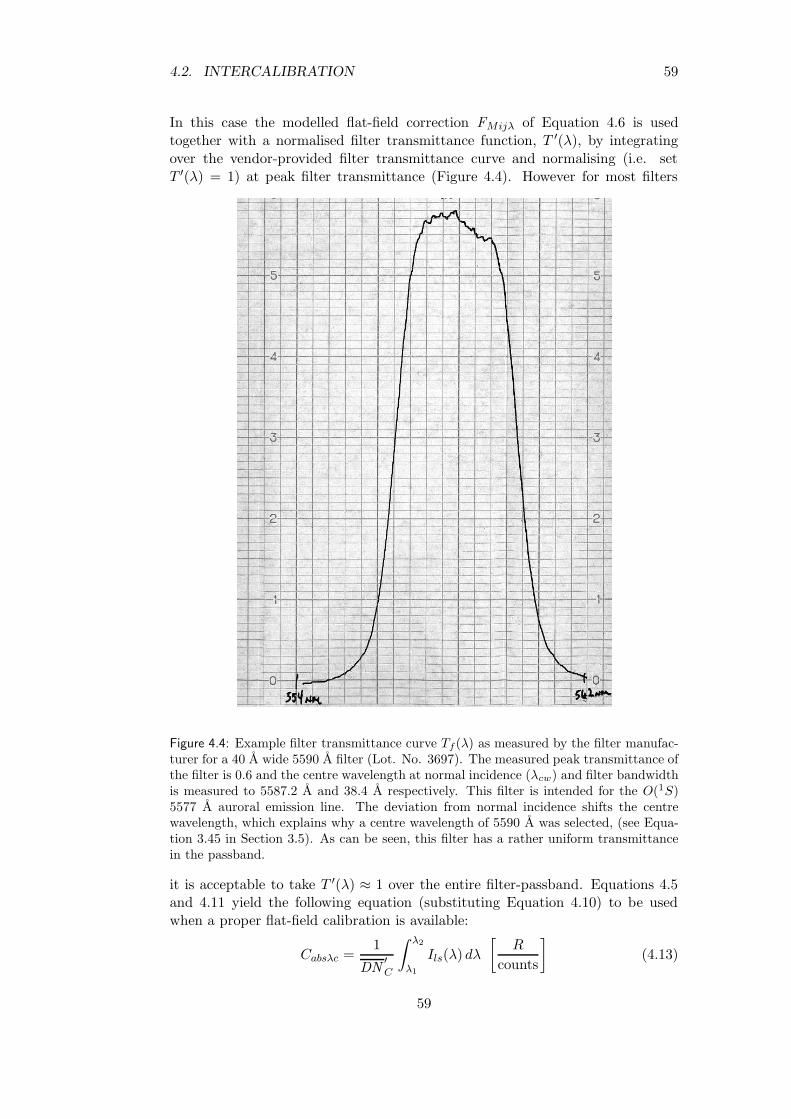
4.2. INTERCALIBRATION 59
In this case the modelled flat-field correction FMijλ of Equation 4.6 is usedtogether with a normalised filter transmittance function, T ′(λ), by integratingover the vendor-provided filter transmittance curve and normalising (i.e. setT ′(λ) = 1) at peak filter transmittance (Figure 4.4). However for most filters
Figure 4.4: Example filter transmittance curve Tf (λ) as measured by the filter manufac-turer for a 40 A wide 5590 A filter (Lot. No. 3697). The measured peak transmittance ofthe filter is 0.6 and the centre wavelength at normal incidence (λcw) and filter bandwidthis measured to 5587.2 A and 38.4 A respectively. This filter is intended for the O(1S)5577 A auroral emission line. The deviation from normal incidence shifts the centrewavelength, which explains why a centre wavelength of 5590 A was selected, (see Equa-tion 3.45 in Section 3.5). As can be seen, this filter has a rather uniform transmittancein the passband.
it is acceptable to take T ′(λ) ≈ 1 over the entire filter-passband. Equations 4.5and 4.11 yield the following equation (substituting Equation 4.10) to be usedwhen a proper flat-field calibration is available:
Cabsλc =1
DN′
C
∫ λ2
λ1
Ils(λ) dλ
[
R
counts
]
(4.13)
59
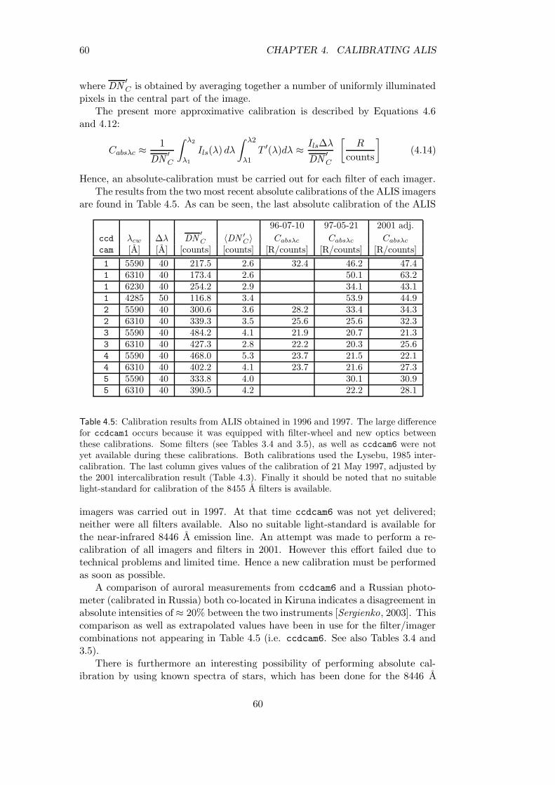
60 CHAPTER 4. CALIBRATING ALIS
where DN′C is obtained by averaging together a number of uniformly illuminated
pixels in the central part of the image.The present more approximative calibration is described by Equations 4.6
and 4.12:
Cabsλc ≈1
DN′C
∫ λ2
λ1
Ils(λ) dλ
∫ λ2
λ1T ′(λ)dλ ≈ Ils∆λ
DN′C
[
R
counts
]
(4.14)
Hence, an absolute-calibration must be carried out for each filter of each imager.The results from the two most recent absolute calibrations of the ALIS imagers
are found in Table 4.5. As can be seen, the last absolute calibration of the ALIS
96-07-10 97-05-21 2001 adj.
ccd λcw ∆λ DN′
C 〈DN ′
C〉 Cabsλc Cabsλc Cabsλc
cam [A] [A] [counts] [counts] [R/counts] [R/counts] [R/counts]
1 5590 40 217.5 2.6 32.4 46.2 47.41 6310 40 173.4 2.6 50.1 63.21 6230 40 254.2 2.9 34.1 43.11 4285 50 116.8 3.4 53.9 44.92 5590 40 300.6 3.6 28.2 33.4 34.32 6310 40 339.3 3.5 25.6 25.6 32.33 5590 40 484.2 4.1 21.9 20.7 21.33 6310 40 427.3 2.8 22.2 20.3 25.64 5590 40 468.0 5.3 23.7 21.5 22.14 6310 40 402.2 4.1 23.7 21.6 27.35 5590 40 333.8 4.0 30.1 30.95 6310 40 390.5 4.2 22.2 28.1
Table 4.5: Calibration results from ALIS obtained in 1996 and 1997. The large differencefor ccdcam1 occurs because it was equipped with filter-wheel and new optics betweenthese calibrations. Some filters (see Tables 3.4 and 3.5), as well as ccdcam6 were notyet available during these calibrations. Both calibrations used the Lysebu, 1985 inter-calibration. The last column gives values of the calibration of 21 May 1997, adjusted bythe 2001 intercalibration result (Table 4.3). Finally it should be noted that no suitablelight-standard for calibration of the 8455 A filters is available.
imagers was carried out in 1997. At that time ccdcam6 was not yet delivered;neither were all filters available. Also no suitable light-standard is available forthe near-infrared 8446 A emission line. An attempt was made to perform a re-calibration of all imagers and filters in 2001. However this effort failed due totechnical problems and limited time. Hence a new calibration must be performedas soon as possible.
A comparison of auroral measurements from ccdcam6 and a Russian photo-meter (calibrated in Russia) both co-located in Kiruna indicates a disagreement inabsolute intensities of ≈ 20% between the two instruments [Sergienko, 2003]. Thiscomparison as well as extrapolated values have been in use for the filter/imagercombinations not appearing in Table 4.5 (i.e. ccdcam6. See also Tables 3.4 and3.5).
There is furthermore an interesting possibility of performing absolute cal-ibration by using known spectra of stars, which has been done for the 8446 A
60
4.2. INTERCALIBRATION 61
emission-line [Gustavsson, 2003]. This method would simplify the calibration pro-cedures considerably. However this is a new method and these results have yetto be intercalibrated with the present calibration method. Regardless of whetherthe new method will be a verification procedure, or replace the present calibra-tion procedure, it will no doubt represent a major improvement of the absolutecalibration for ALIS.
Due to the inherent difficulties of absolute intensity calibration, an error ofthe order of 50 % is often regarded as acceptable. The largest errors appear tobe related to the intercalibration of the light-standards (about 10–20 %, refer toTable 4.4). Furthermore, the calibration results appear to be fairly stable overone year (Table 4.5). On the other hand there are still many uncertain factors inthe calibration procedure, most notably the absence of a uniform source neededfor the flat-field calibration (Section 4.1.3). Therefore, to be on the safe side, itmight be stated that the absolute calibration error lies in the range of 25–50 %.The intercalibration error of the ALIS imagers is probably much lower, at leastfor pixels in the central region of the image. For an imaging instrument, theseerrors are probably to be considered as acceptable. However improvements arestill required.
Finally, the absolute calibration is applied to the object-images (DN ′ij, see
Equations 4.5 and 4.6):
Iij = CabsλcDN ′ij − Ibg,ij [R] (4.15)
In this equation, Iij is the calibrated pixel-value, and Ibg,ij is the sky backgroundcorrection.
4.2.2 Removing the background
Different schemes are employed to remove the sky background in Equation 4.15,depending on available data and the measurement situation. Therefore back-ground removal is only outlined here.
In the case of HF pump-enhanced aurora, linear interpolation with time issometimes used. Also a polynomial could be fitted line by line on each side ofthe emission region. In the most recent papers (Section 6.4) weighted sums ofkeograms through the emission region and on the side of it are used. This is doneunder the assumption that there is no aurora.
Regarding PSC studies (Section 6.6.1), brute-force median/min. filtering wasapplied [Enell , 2002].
For general auroral studies, background determinations are extremely diffi-cult, as there is always some diffuse aurora present. In this case backgroundimages must be obtained by using a filter for a wavelength region with no auroralemissions. For the ALIS imagers, background filters are available: 5100 A and6230 A. However these filters have seldom been used as they are only present atsome stations (Section 3.5). For the future, permanent background photometersmight be a solution of the problem.
61

62 CHAPTER 4. CALIBRATING ALIS
4.2.3 Related issues
On-chip binning
The absolute calibration has been found to scale accurately with the binningfactors, thus:
Cabsλc,binxy =Cabsλc
xbin × ybin
(4.16)
Where Cabsλc,binxy is the absolute calibration constant with binned pixels, xbin isthe binning-factor in the x-direction, ybin is the binning factor in the y-direction.
Linearity
As no variable light-standard is available, the linearity has been checked by vary-ing the integration time (tint). As expected, the CCD detector appears to be com-pletely linear until it reaches the saturation-equivalent exposure (Section 3.1.10).
Interference filters
Both the transmission characteristics and passband of a narrow-band interferencefilter are subject to aging effects. The filter-wheels of the ALIS imagers are alsosometimes subject to high temperatures due to day-time sunlight. This is knownto have a permanent degenerative effect on the filters. Questions have thereforebeen raised regarding the long-term stability of the filters. To clarify these issues,it would be desirable to re-measure filter characteristics for the filters. This wasplanned for the autumn of 2001, but had to be postponed for a number of reasons.
Another concern is to measure the transmittance of the filter, Tf (i, j, λ), asa function of pixel indices, (i, j), (columns, lines). A monochromator systemfor filter transmission measurements was developed for ALIS [Vaattovaara andEnback , 1993]. Provided that an ALIS imager has a valid flat-field calibration, itshould in principle be possible to check the transmittance of the optical system(including the filter) as a function of wavelength and pixel coordinates. Such astudy would be beneficial for all optical instruments, using interference filters, andcould provide answers to questions posed by Kaila and Holma [2000] regardingabsolute calibration of wide field-of-view photometers and camera systems.
4.3 Geometrical calibration
The task of mapping the field-of-view of each pixel to the observed object is calledgeometrical calibration. As this topic is extensively covered in Gustavsson [2000,Chapter 4–5] it will only be briefly touched upon here. First a set of star-imagesare obtained for the viewing direction under consideration. Then the positions ofthe stars are calculated from a star-catalogue (Bright Star Catalogue (BSC))∗ andmapped down to the image coordinates. Then preferably more than 100 stars,evenly distributed across the image, are identified. Finally a transfer function isadjusted so that the calculated and actual positions of the stars overlap. This
∗ftp://adc.gsfc.nasa.gov/pub/adc/archives/catalogs/5/5050
62

4.3. GEOMETRICAL CALIBRATION 63
transfer function is then used for calculating the field-of-view of each pixel of theCCD. Table 4.6 displays the fields-of-view of the ALIS imagers as calculated fromthe transfer-function.
field-of-viewccdcam FoVo FoVx FoVy
1 90.4 59.3 × 60.5
〈FoV〉 1.2 1.1 0.9
2 71.8 48.5 × 48.7
〈FoV〉 0.2 0.1 0.1
3 71.7 48.8 × 48.8
〈FoV〉 0.1 0.6 0.3
4 72.2 49.9 × 49.6
〈FoV〉 0.1 0.1 0.1
5 71.8 49.6 × 49.1
〈FoV〉 0.2 0.2 0.1
6 102.1 66.1 × 68.6
〈FoV〉 1.1 0.4 0.2
Table 4.6: Measured fields-of-view for the ALIS imagers. These values are obtained fromthe geometrical calibration procedure using star images. Note that the CCD is a squareinscribed in a circular field-of-view. Also note that the fields-of-view are calculated in aspherical geometry.
The optics used for the ALIS imagers is aberration limited, rather than dif-fraction limited. The effect of this aberration limited focus is shown in Figure 4.5.As can be seen the point spread function varies over the image plane, from 1–2pixels in the centre to a few pixels at the edges. This will smoothen and widenimages of sharp and narrow structures, in particular in the corners of the images.At the present no attempts are made to deblur/sharpen the effect of the PSF[Gustavsson, 2000, pp. 46–47].
63
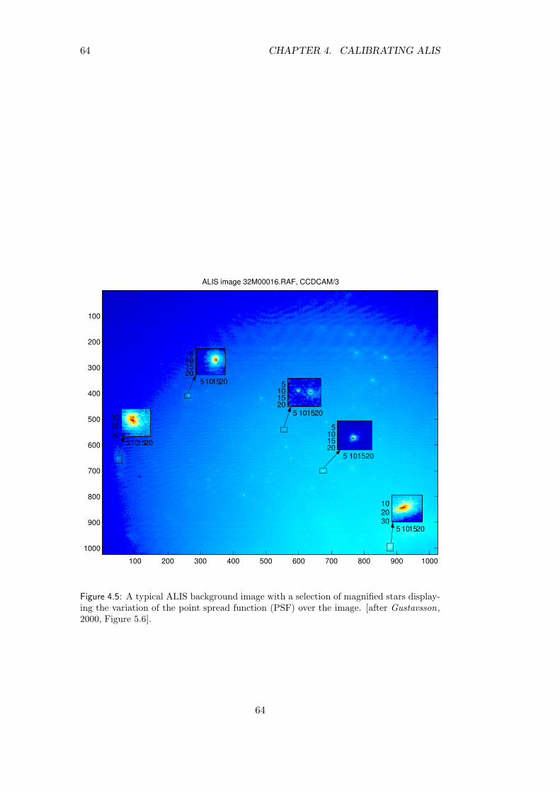
64 CHAPTER 4. CALIBRATING ALIS
ALIS image 32M00016.RAF, CCDCAM/3
100 200 300 400 500 600 700 800 900 1000
100
200
300
400
500
600
700
800
900
1000
5101520
102030
5101520
5101520
5 101520
5101520
5 101520
102030
5 101520
5101520
Figure 4.5: A typical ALIS background image with a selection of magnified stars display-ing the variation of the point spread function (PSF) over the image. [after Gustavsson,2000, Figure 5.6].
64
65
Chapter 5
Controlling ALIS
“For the highest payoff per dollar risked it should be remembered that com-munication system development is normally a ten year leadtime cycle pro-cess. Much better work in this field appears to result from a small numberof people working for a long period of time than from a large massive crasheffort attempting to generate a complete system within short time”
F. R. Collbohm
Software for ALIS falls into two main categories: data analysis software (Sec-tion 6.2) and software for controlling ALIS. In the early phase of work on ALIS,initial ideas for how to develop the software for controlling ALIS were discussedby Steen et al. [1990]; Johansson [1991]; Nilsson and Nystrom [1992] and Nilsson[1994]. While the main ideas for the control centre software have been in useuntil now, this is not the case for the station software.
ALIS is a complex and highly configurable instrument compared to traditionalground-based auroral imaging equipment. Someone once remarked that “com-paring ALIS with a traditional all-sky camera is like comparing EISCAT with anionosonde”. ALIS is a campaign-orientated instrument and therefore needs moreattention prior to measuring compared to traditional imagers. This gives largeamount of flexibility for performing new types of scientific studies, but also intro-duces new problems. First of all, ALIS is a new instrument, with new and partlyunexplored possibilities, and to learn those possibilities takes long time. Whileabsolute measurements from photometers have been analysed for almost half acentury, there is no common established practice to deal with such data expandedto two dimensions (not to mention three dimensions). Traditionally images havebelonged to the realm of morphological measurements (some exceptions exist).Another concern is the tremendous increase in the amount of data produced, andhow to process and analyse the data in a way that enables and improves the pos-sibilities for physical interpretation. The point of this discussion is simply that itis difficult to develop a control system for something that is to a large extent newand unknown. Other difficulties arise from technical limitations, as well as fromthe rapid technical development, causing some components to become obsoletebefore they are finished and making it difficult to put priorities in the right order.(In the beginning of the project various proprietary programming environmentshad to be procured and learned, often at a high cost. Some years later, morestandardised, reliable and free software emerged, partly making the earlier efforts
65
66 CHAPTER 5. CONTROLLING ALIS
superfluos. If that had been known in advance, those resources could have beenspent on other tasks.) The development of a control system for ALIS was there-fore carried out by successive approximation and “survival of the fittest” ideas.The following sections will provide a brief overview of a vast subject that is bestdescribed by running ALIS and studying the source code.
5.1 Making an observation with ALIS
Experience has suggested the following steps for configuring ALIS for an obser-vation:
1. Defining a scientific rationale: This is of course the first and most im-portant task. Naturally it is almost impossible to predict the outcome ofany observations. Nevertheless, well planned measurements with a clearview of what needs to be done tend to yield better results than “ad hoc”operations.
2. Selecting stations: Normally it is best to use as many stations as possible,but there might be observation schemes that require only a subset of thestations. It is also important to plan what changes to the rationale arenecessary in case some stations cannot take part in the observation (forexample due to clouds or technical problems).
3. Selecting imager viewing directions: This can be either the standardpreset viewing-directions (Figure 3.11 and Table 3.6) or specially calculatedviewing directions for a particular measurement. It is advisable to preparea strategy for possible changes if the observed phenomena moves outside ofthe field-of-view. In most cases it is best to avoid changes of the viewingdirections during a measurement. “Chasing the aurora” usually results inpoor data. Another concern is to make sure that the selected positions aregeometrically calibrated against the star background (Section 4.3).
4. Selecting filters: Filter selection usually follows directly from the scientificrationale. However all filters are not available at all stations (see Tables 3.4and 3.5). Filter change time increases with the distance between the filterson the filter-wheel (nominally 1–2 s). It might also be necessary to obtainbackground intensities by exposing images with background filters.
5. Selecting integration times: The minimum integration time is defined bythe shortest exposure resulting in an acceptable SNR. As the spectral sens-itivity varies for the imager, there is normally a need for longer exposuresfor shorter wavelengths. Maximum exposure is defined by the longest ex-posure without saturating the CCD, or, more frequently, by requirementsset by the desired temporal resolution. The risk of saturating the CCD mustbe considered at high binning factors as the sensitivity increases with thebinning factors (Figure 3.4). Occasional saturated images pose no threat tothe CCD, but yield unusable data. Finding an optimal integration time hasproven to require large amounts of experience from earlier measurements.(see also Chapter 3)
66
5.1. MAKING AN OBSERVATION WITH ALIS 67
6. Selecting temporal resolution: The temporal resolution is currently lim-ited to one image per 30–60 s at maximum resolution, and is generally neverbetter than 30 images per minute at higher binning factors. These figuresvary somewhat between the imagers. Also times for filter changes must beconsidered.
7. Selecting spatial resolution and sensitivity: This is generally a compro-mise between temporal resolution, sensitivity, framerate and disk-space.Note that increasing the temporal resolution by binning might lead to sat-uration problems due to the increase in sensitivity.
8. Deciding on data storage strategies: As the disk space at the stationsis limited, it is advisable to estimate the amount of data produced anddecide what data should be kept, when to retrieve the data and if deletingpresumed unusable images should be allowed, etc.
9. Coordination with other instruments: Such as EISCAT measurements,satellite passes, rocket launches etc. This involves many considerations (forexample when does a satellite pass occur? Should ALIS image along thefoot-point of the satellite pass?). It is also essential to establish communic-ation with the control centres of participating facilities.
10. Selection of a suitable operational mode for the observation:Available modes are: automatic, semiautomatic or manual, see Sec-tion 5.1.1. In order to increase the number of observations of a particularphenomenon it would be desirable to have more automatic runs, however,experiences indicate that at the present, the best results emerge frommanned semiautomatic runs.
11. Defining and testing the required configuration of ALIS: No us-able bug-free program exists. Therefore everything should be tested asthoroughly as possible before running the actual observation. It is alsoimportant to start up all systems in ALIS well in advance. The imagersneed to be thermally stable and defrosting of the domes as well as bootingsubsystems at the stations might also take some time. (Estimate at least1–2 days for testing a new measurement scheme, and 2–4 hours to startup ALIS.) It is also advisable to perform some rudimentary last checkoutprocedures about one hour prior to starting the measurements.
12. Waiting for the right conditions: This might be a long wait. In thisphase, it is advisable to take images at all stations at regular intervals tocheck weather conditions and system performance. It is also a good practiceto be prepared for many different kinds of observations. For example, ifconditions for observing HF-pump enhanced airglow are not right, theremight be an excellent auroral event instead.
13. Run the observation: During measurements many unexpected things canhappen, so it is good to be well-prepared with alternatives. Two to threepeople in the control centre are the ideal for most measurements: one whotakes care of technical problems and runs the system, one who concentrates
67
68 CHAPTER 5. CONTROLLING ALIS
on taking scientific decisions and possibly one who coordinates with otherinstruments. Taking good notes is essential, as analysis might not occuruntil months later.
14. Retrieve the raw-data from the stations: It is time-consuming to re-trieve raw-data from the stations. All six stations can be visited in less thana week, but this requires a lot of driving. Usually the disks are brought backonly during scheduled maintenance trips to the stations, or as the disks be-come full. If exceptionally interesting data have been recorded, it mightstill be desirable to retrieve it as quickly as possible.
15. Analysing and publishing the results: First one needs to select data,then this data-set must be preprocessed and calibrated before the actualanalysis and publication phase starts. These final steps rely on good record-keeping in the previous steps.
5.1.1 Modes of operation
The modes for controlling ALIS are summarised below:
Manual control: By sending commands directly to ALIS, a user is able to con-trol observations interactively. This mode of operation is most frequentlyused for checking observing conditions (cloudiness, etc.), for troubleshoot-ing and for maintenance.
Semiautomatic operation: In this mode a user controls ALIS by running ob-servation control programs (usually these are shell-scripts at the stations)that are uploaded, prepared and tested in advance. This is the normaloperating mode.
Automatic operation: In this mode, an observation control program is loadedand run automatically at a predefined time. This mode can easily beswitched to semi-automatic mode if the user wishes to change anything.Exceptions can be reported using a paging system if the control centre isunmanned. Due to the vast amounts of data produced, automatic meas-urements are uncommon.
5.1.2 Alarms and other exceptions
Many exceptions can be properly acted upon automatically, while others requiremanual interaction. These exceptions trigger alarms, which are displayed atALIS-CC and at all user interfaces. If user interface is active, an automaticpaging system will also alert the operator on duty. Typically, a pager call occursfor A-Alarms or fatal alarms, (see below) but the paging system can be configuredto alert a user when an interesting measurement situation is emerging, etc. ALISexceptions are classified in three alarm categories:
Fatal alarms: Fire, trespass or other severe conditions threatening the hard-ware.
68

5.2. OPERA 69
A-Alarms: Conditions causing the imaging to stop at one or several stations(power failures, filter-wheel problems, unrecoverable run-time errors, etc.).
B-Alarms: Other conditions affecting the quality of observations (timing prob-lems, communication problems, over- or under-exposed images, etc.).
5.2 OPERA
The complete collection of software for controlling ALIS is called an OPERationssystem for ALIS (OPERA). The three main components of OPERA are brieflydescribed below.
5.2.1 User interfaces
The main graphical user interface for ALIS is an X-windows application(parsifal) that has been supported on various computing platforms (HP-UX,Sun-OS (Solaris), GNU/Linux, Windows-95 and Java). It provides a user-friendlyway to configure and run ALIS as well as to display quick-looks and status in-formation. Commands can be sent to the system, either by user-defined menus ordirectly by typing them on a command line. From parsifal it is possible to mon-itor and control ALIS in many ways, to receive and view quick-look images, tocommunicate with other ALIS users, to upload experiment configurations, etc.. Atext-only user interface, (tosca), is available for controlling ALIS over slow com-munication lines (implemented in Lisp as a major mode for the Emacs editor).From around 1999, as the stations become networked over ppp (Section 2.2.3) italso became possible to configure and control the stations over direct TCP/IPconnections (for example by making a direct telnet login to the desired stationcomputer). It is foreseen that the need for a dedicated control centre and specialuser-interfaces will vanish as it will be possible to control ALIS from an ordinaryweb-browser in the future.
5.2.2 AIDA
A central set of server processes, Alis Internal Data Administration (AIDA) runsat the control centre, accepting connections from user interfaces and directinguser-commands to the desired set of stations. Furthermore, requests from thestations affecting users, or other stations, are routed to their proper destinations.AIDA also handles alarms and other exceptions and activates the paging systemif no user-interface is online. The concept of AIDA as a central node (or crossbar-switch) has survived since the first implementation (around 1992), but is subjectto change in the future as all stations become networked. When this happens, acentral node is no longer required, as this functionality can be undertaken by anystation. Therefore the need for a dedicated control centre will also diminish withtime. All of the AIDA software was written in a Unix/C environment from thebeginning, first under HP-UX and later ported to GNU/Linux. A block-diagramof the AIDA software and user interfaces appears in Figure 5.1. See [Nilsson,1994] for a more detailed description of AIDA.
69

70 CHAPTER 5. CONTROLLING ALIS
V
RRR
G
R
S04S03 S05 S06
RR
S02
R
S01
AIDA
CC−map
User Interfaces:Tosca Parsifalssh Parsifal http:
Figure 5.1: Block diagram of OPERA. Any number of user-interfaces (parsifal, tosca)can connect to AIDA in order to control ALIS. In AIDA a central supervising process V(verdi) routes all information between the different user-interfaces and the stations. Thestations are connected to verdi via an interface process, R (radames controls a RS-232serial line and a modem, or rigoletto that provides a TCP/IP connection to a stationover an existing network connection). The control centre status display map (Figure 2.7)is connected in the same way as an ALIS station. The user-interfaces labeled ssh andhttp indicate the possibility to control the stations over a shell-login, or from a standardweb-browser. This will eventually make the control centre software superfluous, as thefunctionality of AIDA will be available at each station.
70
5.2. OPERA 71
5.2.3 Station software
The present ALIS stations are to a large extent controlled by station-control pro-grams running in the station computer (SC). As long as MS-DOS was used asthe operation system for the station computer (Section 2.2.6) a huge applicationprogram (HENRIK) controlled the station. Due to the many and absurd tech-nical limitations of MS-DOS, this program had problems meeting the requiredspecifications, especially with respect to speed, reliability and the data-handlingcapacity. As GNU/Linux emerged as a reliable and free multi-tasking operatingsystem, it was quickly realised that a change of operating-system at the stationswas top priority. Around 1997, HENRIK was quickly ported to GNU/Linux; theresulting program was called arnljot. Although this was a major improvement,it was still a ported huge MS-DOS program including large amounts of code writ-ten exclusively to bypass MS-DOS limitations. To remedy this, a major rewrite ofthe code was initiated, removing all “MS-DOS-artifacts”, as well as splitting theprogram in three parts: aniara handling the overall station control and commu-nication with the control centre; mima, controlling the imager; and nipu handlingthe NIPU, (Section 2.2.2). These programs have been in routine operation since1999.
aniara supervises most functions at the station and provides an interface toAIDA. Among many other things, aniara handles alarm conditions, storesconfigurations, and acknowledges “sanity-checks” sent from the Housekeep-ing Unit (Section A.4) after verifying that the station computer is operatingproperly. A simple text-oriented user interface to ALIS, mainly intendedfor system maintenance is also provided by aniara. As AIDA is slowlyphased out, aniara will most likely take over some of its functionality.
mima is the imager control program. It boots up the camera-control unit (Sec-tion 3.3.2), configures the imager (Section 3.3.3), retrieves the image-dataas well as creates and saves FITS images onto the local disks (Section 2.2.5).This program is thus responsible for putting all the supplementary informa-tion into the FITS header (integration-time, filter, UTC, viewing direction,CCD-temperatures, etc.).
nipu is a program for controlling and booting the NIPU. This program is usedto calibrate the FPS and CPS, select filters (Section 3.5) and viewing-directions (Section 3.6).
Apart from the software discussed above, it is also worth mentioning the followingsoftware packages at the station:
CCU-software: Vendor-provided Transputer binaries for the camera-controlunit (Section 3.3.2). This code is uploaded by mima during the imagerboot-up phase.
HU-firmware: The Housekeeping Unit (Section A.4) firmware is written inassembler and stored in an Erasable Programmable Read-Only Memory(EPROM). It provides low-level interfaces to various GLIP systems (Ap-pendix A), watchdog functions for the station computer, as well as alarm
71
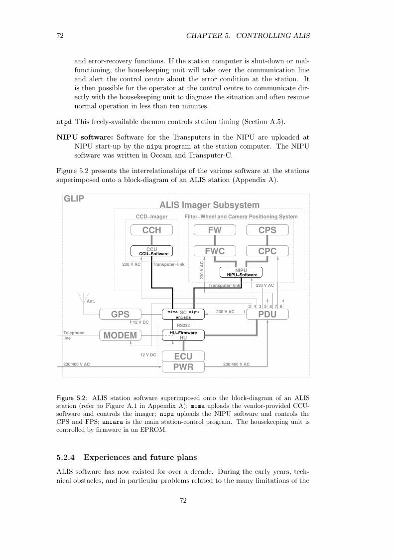
72 CHAPTER 5. CONTROLLING ALIS
and error-recovery functions. If the station computer is shut-down or mal-functioning, the housekeeping unit will take over the communication lineand alert the control centre about the error condition at the station. Itis then possible for the operator at the control centre to communicate dir-ectly with the housekeeping unit to diagnose the situation and often resumenormal operation in less than ten minutes.
ntpd This freely-available daemon controls station timing (Section A.5).
NIPU software: Software for the Transputers in the NIPU are uploaded atNIPU start-up by the nipu program at the station computer. The NIPUsoftware was written in Occam and Transputer-C.
Figure 5.2 presents the interrelationships of the various software at the stationssuperimposed onto a block-diagram of an ALIS station (Appendix A).
NIPU
FW CPS
FWC CPC
Filter−Wheel and Camera Positioning System
230
V A
C
230 V ACTransputer−link
CCU
Transputer−link
CCH
230 V AC
CCD−Imager
ALIS Imager Subsystem
SC
HU
PWRECU
PDU12 4 8 7 653
MODEMTelephoneline
GPS
230/400 V AC 230/400 V AC
12 V DCRS232
230 V AC
CCU−Software
Ant.
NIPU−Software
mima nipuaniara
HU−Firmware
GLIP
12 V DC
Figure 5.2: ALIS station software superimposed onto the block-diagram of an ALISstation (refer to Figure A.1 in Appendix A); mima uploads the vendor-provided CCU-software and controls the imager; nipu uploads the NIPU software and controls theCPS and FPS; aniara is the main station-control program. The housekeeping unit iscontrolled by firmware in an EPROM.
5.2.4 Experiences and future plans
ALIS software has now existed for over a decade. During the early years, tech-nical obstacles, and in particular problems related to the many limitations of the
72
5.2. OPERA 73
operating system at the stations, dominated. Following the major OS upgrade toGNU/Linux, most of these software problems have now been eliminated. The im-portance of reliable and free operating systems cannot be over-estimated. Manyman-years of programming efforts could have been saved if proprietary softwarecould have been avoided in the first place.
Regarding the user-interfaces, it seems inevitable that an effort will be re-quired to create a web-oriented standard user interface for ALIS. AIDA willprobably be depreciated in favour of moving this functionality to the stations.This will also increase redundancy of the ALIS control system. At the stationsa simple and flexible approach seems to be to let each major functionality tobe represented by an application program. An interesting development is thenetworked “parameter-server” that can be used to configure ALIS as well as toretrieve status information in a consistent way over the entire network of stationsand user-interfaces.
The lag between the desired and present control system for ALIS is in theorder of 1–2 man-years. Finally it should never be forgotten that software devel-opment is an evolutionary process that requires continuous upgrades and main-tenance.
73

74 CHAPTER 5. CONTROLLING ALIS
74
75
Chapter 6
Scientific results from ALIS
“Vetenskapsmannen ar en byggmastare. Att samla vetenskapliga uppgifterkan jamforas med att samla stenar till ett hus; en hog med uppgifter ar intemer “vetenskap” an en hog stenar ar ett hus. Obearbetade vetenskapligaresultat ar bara en dod stenhog” Kristian Birkeland
“Wovon man nicht sprechen kann, daruber muß man schweigen”Ludwig Wittgenstein
This chapter attempts to provide a summary of the scientific results obtainedfrom the analysis of data from ALIS. It is important to stress that this canonly be a brief review of published scientific results in order to demonstratethe scientific applicability of ALIS in particular, and of multi-station imaging ingeneral. The reader is urged to read the original papers for more complete anddetailed information about the scientific results summarised.
Interesting results often emerge from unexpected directions. HF pump-enhanced airglow was not mentioned among the scientific objectives in the earlyALIS papers. However, this topic existed as an auxiliary scientific objective until16 February 1999, when the first unambiguous observations of this phenomenonat high-latitudes were made. Since then it has been the main scientific objectiveof the ALIS measurements. Hence, a large portion of this chapter (Section 6.4)is therefore devoted to these observations.
It is essential for a proper interpretation of the data-sets to do coordinatedobservations involving as many independent measurement systems as possible.ALIS has participated in a number of coordinated campaigns involving instru-mentation such as the tri-static European Incoherent SCATter radar (EISCAT),the EISCAT Heating facility in Tromsø, the American FAST, POLAR and MSXsatellites, and the German lee-wave campaign studying polar stratospheric cloudsetc.
The author’s main role has been to supervise and make the observations withALIS and supporting instruments, retrieve, calibrate and validate the datasets,as well as to assist with data-analysis and interpretation of the data-sets. MostALIS data-analysis software, and in particular the software for triangulation andtomography-like analysis has been designed and written by Bjorn Gustavsson.He also performed most of the data-analysis. Many other coauthors (see thebibliography) contributed to the physical interpretations of the data-sets obtained
75
76 CHAPTER 6. SCIENTIFIC RESULTS FROM ALIS
from ALIS. This division of responsibilities appeared naturally in a small groupwith a large and technically complex project.
6.1 Scientific objectives of ALIS
The list below tries to summarise the scientific objectives of ALIS, from the firstproposal [Steen, 1989] until the present time.
Non-stable auroral forms: Auroral events such as: substorm onsets, West-ward Travelling Surges (WTS), surges, folds, spirals (or auroral vortices),rays and omega bands, and the not well-understood pulsating and flicker-ing aurora belong to this category. These phenomena require observationswith high temporal and spatial resolution. So far, ALIS has been usedinfrequently to make this type of observations, due to a combination oftechnical limitations (Section 3.3.4), as well as difficulties related to thescientific understanding of these phenomena. However, a theoretical paperon auroral vortices was published (Section 6.5.3).
Stable auroral forms: The stable auroral arc has been the topic for many stud-ies during the last five decades. Despite this, the ionospheric environmentin and around it is not yet fully understood. Detailed field-aligned meas-urements of ionospheric parameters combined with tri-static plasma-driftmeasurements by EISCAT, produce profiles on electron density, electronand ion temperatures ranging from some 90 km to 1000 km, as well as, ho-rizontal electric-field estimates in the ionospheric F-region. To relate suchmeasurements to the optical data from ALIS, as well as to satellite andother ground-based instruments would increase the scientific yield of stud-ies of stable auroral forms. Some results of such coordinated observationswith ALIS, EISCAT and the FAST satellite are discussed in Section 6.5.2.Another stable auroral form is the diffuse aurora, (added to the scientificobjectives in Steen et al. [1990]) where the equatorward edge of the dif-fuse aurora has been used to estimate the size of the auroral oval. Themain ionospheric trough is often associated with the equatorward edge ofthe auroral oval. Examples of “accidental” measurements of the trough arediscussed in Section 6.5.4. Other studies (however, not always of stableaurora) that could be included here are : enhanced aurora [Hallinan et al.,1985], black aurora, statistical studies of arc-thickness etc.
Characteristic energy of particles: By the use of spectroscopic ratios, thecharacteristic energy of the precipitating particles can be obtained [Hechtet al., 1989; Meier et al., 1989; Strickland et al., 1994; Rees and Luckey ,1974]. To do this properly would require simultaneous measurements attwo wavelengths at each station, thus doubling the data-flow and requiringat least two imagers at each station. Results obtained so far involve a singlecamera at each station and rapid filter changes (Section 6.5.1).
A 3-D image: Since the fields-of-view of the ALIS stations overlap, it is pos-sible to estimate the altitude distribution of auroral emissions by utilisingtriangulation and tomographic inversion techniques. Steen [1989] expected
76
6.1. SCIENTIFIC OBJECTIVES OF ALIS 77
that ALIS would be able to produce 2-D maps of the altitude-distributionof the different auroral emissions. This would represent a pseudo 3-D imageof the aurora. To develop techniques for visualising the variations in timeand space of 3-D aurora was characterised as “an interesting but non-trivialexercise∗”. While the latter still lies in the realm of the future, ALIS-imageshave frequently been used for obtaining heights and volume distributionsthrough triangulation and tomography-like inversion techniques. The pro-gress in this field is reported in Section 6.3 and references therein.
Relation between electron and proton aurora: The main auroral particlespecies are electrons and protons. The intensity of the more diffuse protonaurora is much lower than the electron aurora. In order to study the relationbetween these two types of aurora, it was suggested to use the N +
2 1Neg.(4278 A) and Hβ (4861 A) emission lines [see for example Galand , 2001,and references therein]. Although ALIS would be well-suited for studies ofproton aurora, no measurements have been carried out to date.
The relation between the neutral wind and the aurora: Auroral intensi-fications appear to be related to rapid variations in the thermospheric neut-ral wind on a time scale which excludes contribution from the ion-drag force.This objective was added in Steen et al. [1990] and some initial studies werecarried out (Section 6.5.6).
Non-auroral studies: It was envisioned that ALIS would make mainly auroralobservations during dark periods. The system would also be available forother types of measurements. One such type of measurement is to studythe formation of Polar Stratospheric Clouds (PSC) which is important forthe understanding of ozone depletion. The results of some of these studiesare summarised in Section 6.6.1. It was later proposed [Steen et al., 1990]to study gravity wave modulation of airglow emissions. However, no suchstudies have been carried out to date. It was also speculated that ALIScould be used for other studies, for example high-altitude flashes, cloudsand comets, etc. ALIS acquired some images of the Hale-Bopp and theHyakutake comets; however these data have not yet been analysed. Insummary, observations of HF pump-enhanced airglow quite unexpectedlyended up as the main topic for ALIS.
The majority of published ALIS results to date concerns studies of HF pump-enhanced airglow and therefore constitutes the main part of this chapter. WhenALIS measurements stopped for the season each year due to the midnight sunperiod, one detector participated in a joint study to attempt daytime auroral ima-ging using an imaging spectrometer. This generated some interesting first results,as outlined in Section 6.5.5. Another sidetrack that might become productive inthe future is the study of meteor trails. Some rather promising observations havealready been carried out (Section 6.6.2).
∗The problem is not so much the visualisation itself, but rather that human perception hasevolved to interpret 2-D surfaces of 3-D objects. Evolution has never required an understandingof a true 3-D distribution.
77
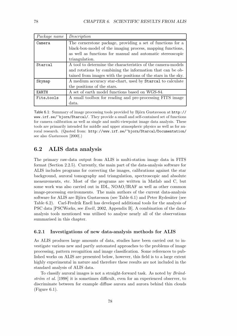
78 CHAPTER 6. SCIENTIFIC RESULTS FROM ALIS
Package name Description
Camera The cornerstone package, providing a set of functions for ablack-box-model of the imaging process, mapping functions,as well as functions for manual and automatic stereoscopictriangulation.
Starcal A tool to determine the characteristics of the camera-modelsand rotations by combining the information that can be ob-tained from images with the positions of the stars in the sky.
Skymap A medium accuracy star-chart, used by Starcal to calculatethe positions of the stars.
EARTH A set of earth model functions based on WGS-84.
Fits tools A small toolbox for reading and pre-processing FITS imagedata.
Table 6.1: Summary of image processing tools provided by Bjorn Gustavsson at http://www.irf.se/~bjorn/Starcal/. They provide a small and self-contained set of functionsfor camera calibration as well as single and multi-viewpoint image data analysis. Thesetools are primarily intended for middle and upper atmospheric physics as well as for au-roral research. (Quoted from: http://www.irf.se/~bjorn/Starcal/Documentation/
see also Gustavsson [2000].)
6.2 ALIS data analysis
The primary raw-data output from ALIS is multi-station image data in FITSformat (Section 2.2.5). Currently, the main part of the data-analysis software forALIS includes programs for correcting the images, calibrations against the starbackground, auroral tomography and triangulation, spectroscopic and absolutemeasurements, etc. Most of the programs are written in Matlab and C, butsome work was also carried out in IDL, NOAO/IRAF as well as other commonimage-processing environments. The main authors of the current data-analysissoftware for ALIS are Bjorn Gustavsson (see Table 6.1) and Peter Rydesater (seeTable 6.2). Carl-Fredrik Enell has developed additional tools for the analysis ofPSC data [PSCWorks, see Enell , 2002, Appendix B]. A combination of the data-analysis tools mentioned was utilised to analyse nearly all of the observationssummarised in this chapter.
6.2.1 Investigations of new data-analysis methods for ALIS
As ALIS produces large amounts of data, studies have been carried out to in-vestigate various new and partly automated approaches to the problems of imageprocessing, pattern recognition and image classification. Some references to pub-lished works on ALIS are presented below, however, this field is to a large extenthighly experimental in nature and therefore these results are not included in thestandard analysis of ALIS data.
To classify auroral images is not a straight-forward task. As noted by Brand-strom et al. [1998] it is sometimes difficult, even for an experienced observer, todiscriminate between for example diffuse aurora and aurora behind thin clouds(Figure 6.1).
78
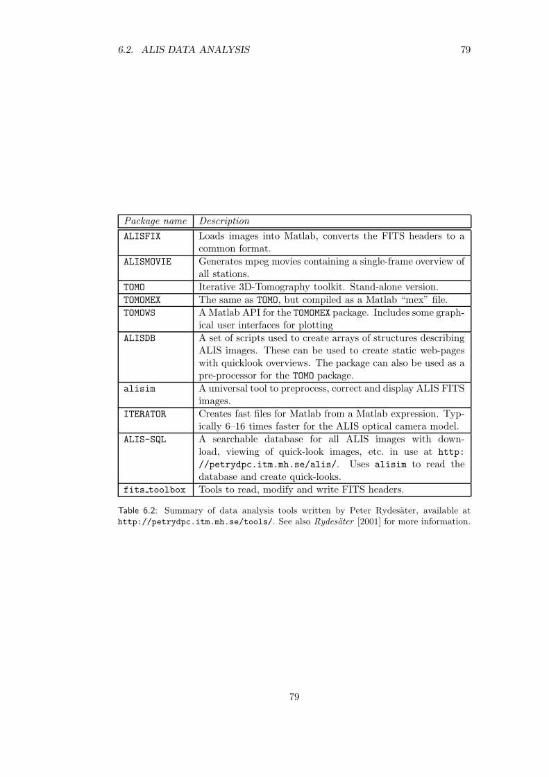
6.2. ALIS DATA ANALYSIS 79
Package name Description
ALISFIX Loads images into Matlab, converts the FITS headers to acommon format.
ALISMOVIE Generates mpeg movies containing a single-frame overview ofall stations.
TOMO Iterative 3D-Tomography toolkit. Stand-alone version.
TOMOMEX The same as TOMO, but compiled as a Matlab “mex” file.
TOMOWS A Matlab API for the TOMOMEX package. Includes some graph-ical user interfaces for plotting
ALISDB A set of scripts used to create arrays of structures describingALIS images. These can be used to create static web-pageswith quicklook overviews. The package can also be used as apre-processor for the TOMO package.
alisim A universal tool to preprocess, correct and display ALIS FITSimages.
ITERATOR Creates fast files for Matlab from a Matlab expression. Typ-ically 6–16 times faster for the ALIS optical camera model.
ALIS-SQL A searchable database for all ALIS images with down-load, viewing of quick-look images, etc. in use at http:
//petrydpc.itm.mh.se/alis/. Uses alisim to read thedatabase and create quick-looks.
fits toolbox Tools to read, modify and write FITS headers.
Table 6.2: Summary of data analysis tools written by Peter Rydesater, available athttp://petrydpc.itm.mh.se/tools/. See also Rydesater [2001] for more information.
79
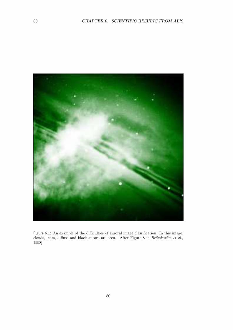
80 CHAPTER 6. SCIENTIFIC RESULTS FROM ALIS
Figure 6.1: An example of the difficulties of auroral image classification. In this image,clouds, stars, diffuse and black aurora are seen. [After Figure 8 in Brandstrom et al.,1998]
80

6.2. ALIS DATA ANALYSIS 81
Auroral classification scheme
Main Secondary Temporal Vortexmorphological morphological feature feature
feature feature
Non-diffuse Active Spiral (E.g. WTS,Diffuse Quiet omega, torch)
Multiple (2,3,. . . ) Pulsating FoldAuroral arc Rayed Curl
one dimension is Striatedsignificantly larger Corona
than the other Dark auroraEnhanced
Partly cloudsIntensity
Non-diffuse Active FoldDiffuse Quiet Curl
Multiple (2,3,. . . ) PulsatingRayed
Fragmental auroral Striatedstructure Corona
Dark auroraEnhanced
Partly cloudsIntensity
Dark aurora PulsatingDiffuse aurora Partly cloudy
covering a larger region Intensity
Unidentified aurora
Table 6.3: An auroral classification scheme (after a proposal by A. Steen) used by themanual classification program for ALIS data. (“Dark aurora” stands for a class of phe-nomena commonly known as “black aurora”)
Early on in the ALIS project, an auroral classification scheme was suggested(by Ake Steen, see Table 6.3). A classification program (developed by PetrusHyvonen and later Mats Luspa) was written. The program was used to manu-ally, but relatively quickly, classify the images according to the classificationscheme in Table 6.3. This classification was very useful but time-consuming dueto the large number of images from many stations. The quality of the image-classification was also dependent on the operator. This classification method wastherefore abandoned, and investigations started to find automated methods ofimage classification.
In an exploratory study carried out by Waldemark et al. [1997]; Eide et al.[1997] Pulse Coupled Neural Networks (PCNN) were evaluated as a preprocessorfor classifying image-data from ALIS. The PCNN is a biologically inspired neuralnetwork based on findings in the visual cortex of small mammals. The algorithmhas been successfully applied in the field of mammography [Kinser and Lindblad ,
81
82 CHAPTER 6. SCIENTIFIC RESULTS FROM ALIS
1997] which, to some extent, possesses similar image processing and classifica-tion problems as encountered in auroral imaging. A three-step procedure forautomatically classifying auroral images is outlined: (1) use a PCNN for imagesegmentation, (2) post-process the resulting data, either by using Singular ValueDecomposition (SVD) or by applying a second PCNN for feature extraction, (3)carry out the actual classification using a traditional neural network. This workwas followed up by Rydesater et al. [1998] who concentrated on the problem ofhow to find auroral arcs, and on their location within the images. For this pur-pose an arc detection algorithm was constructed and tested. Initial attempts weremade to enhance the algorithm with a Radial Basis Neural Network (RBNN). Itwas concluded that the arc detection algorithm gave a robust detection of auroralarcs and their direction. Preliminary results from the application of a RBNN waspromising.
Alpatov et al. [2000] applied self-organising neural networks to ALIS data, forthe detection of polar stratospheric clouds.
A different approach to the problem of automatic recognition of auroral formsis studied by Pudovkin et al. [1998]. Here a more traditional method, based onthe analysis of isolines of auroral luminosity shapes is utilised. Classical formssuch as ellipses, spirals and folds appear to be confidently retrieved. However,Pudovkin et al. [1998] notes that the entire field of auroral classification seems tobe at an early stage: “There are needs for extensive and purposeful studies of theforms peculiar to certain geophysical conditions, with the nature of the physicalprocess within the auroral plasma and their characteristic time and space scalesbeing taken into account.”
Rydesater [2001] presents a survey of possible methods of implementing aSelective Imaging Technique (SIT) functionality in ALIS, as proposed by Steenet al. [1997a]. (This would be an algorithm or a device that automatically controlsALIS, or advises the operator to acquire data of specific interest when favourableconditions occur.)
A study on the effects of lossy compression of auroral image data is presentedin Rydesater et al. [2001]. At least for the images studied, it appears to bepossible to compress images to approximately 5–12% of their original size withoutincreasing errors.
Another topic is the study of the fractal dimension of auroral features. Aninitial study was carried out by Alpatov et al. [1996a,b]. It was concluded thatfractal analysis methods can be used to segment auroral images into aurora,stars, clouds and background. However it remains to be seen if segmentation ofthe auroral features themselves can be related to physical processes responsiblefor the aurora.
Despite the fact that these studies provided promising preliminary results,much work remain before these methods can be applied to auroral imaging on aregular basis.
Apart from the work related to ALIS, many other groups are working inthis field. An example of this is the very promising work by Syrjasuo [2001,and references therein] on auroral detection/classification by automated imageanalysis.
82
6.3. TOMOGRAPHY AND TRIANGULATION 83
6.3 Tomography and triangulation
Many earlier experiments have used multi-station measurements combined withtriangulation techniques to estimate the height of the aurora (Section 1.1.1).Computer Tomography (CT) has its most well-known applications in the field ofradiology† [Cormac, 1963a,b]. A similar method was applied by Solomon et al.[1984] to estimate the airglow distribution as measured by space-borne photomet-ers. An emission distribution was characterised by Jones et al. [1991] by usingdata from a rocket and three ground-based scanning photometers. Na and Lee[1991] estimated ionospheric electron densities from radar measurements by theuse of tomographic methods. McDade and Llewellyn [1994] presented methodsto estimate airglow distributions from limb-scanning satellite measurements. Bythe use of image data from two monochromatic TV-cameras in Antarctica witha separation of 20 km Aso et al. [1990] studied the auroral emission distributionin slices.
6.3.1 Methods, initial studies and simulations
One primary scientific objective of ALIS was to provide the possibility to re-construct the 3D auroral volume emission by applying tomographic inversiontechniques on spectroscopic high-resolution images of aurora, airglow and relatedphenomena [Steen, 1989]. An initial study based on simulated ALIS-data wasperformed by Gustavsson [1992]. Later, the problems of auroral tomographywere discussed during an auroral tomography workshop in Kiruna [Steen, 1993].A more detailed model simulation study [Gustavsson, 1998] concluded that thecapability to achieve results with acceptable horizontal and vertical resolution,exists. This paper also suggests a useful way to define a stopping criteria for iter-ative tomographic methods by combining adaptive low-pass filtering and feasibil-ity tests, and concludes that “it is possible to achieve feasible reconstructions withthe modified Multiplicative Algebraic Reconstruction Technique (MART).” Anintroductory overview of ground-based tomography, including a further investig-ation of resolution and error sensitivity is presented in Gustavsson [2000, Chap.3] concluding that “the result of the tomographic inversion cannot retrieve finescale internal structures. However, estimates of the spatial distribution of iono-spheric emissions which, in general, have a comparatively simple shape, can beaccurately obtained”. The chapter also presents a strengthening of the statisticalstopping criteria of Veklerov and Llacer [1989].
6.3.2 Summary of results from computer tomography of ALIS-data
At an early stage a close scientific and technical collaboration was establishedwith colleagues at Kyoto University, and later at the National Institute for Polar
†Incidentally, the term “tomography” existed in radiological applications decades before com-puterised tomography became a real possibility. See, for example, Lodin [1935]; Weinbren [1946],and other references discussed in Backlund [1956]. Typically a series of X-ray exposures wereobtained while the X-ray tube and film-cassette rotated around the patient. Back then, thetomographic inversion had to be performed by the brain of the radiologist observing these seriesof X-ray images.
83

84 CHAPTER 6. SCIENTIFIC RESULTS FROM ALIS
Research (NIPR), Tokyo. During a joint campaign (ALIS-Japan 1) held in March1996, the first results of auroral tomography were obtained as reported in Asoet al. [1998a]. At this time ALIS had only three imagers, and two additionalintensified CCD-cameras were provided by our Japanese colleagues [Aso et al.,1993, 1994], resulting in a total of five imaging stations. A modified MARTwas used for tomographic analysis, presenting initial results of tomography for afolded arc, and a double-arc system [Aso et al., 1998a]. An auroral model with afolded arc is also discussed in this paper.
In Aso et al. [1998b] initial results and model comparisons using a modifiedversion of a Simultaneous Iterative Reconstruction Technique (SIRT) [Gilbert ,1972] were applied to data from the March 1995 ALIS-Japan 1 campaign. Themethod was also verified by numerical simulations. An auroral fold occurringat 23:40:30 UTC on 26 March 1995 was selected for testing the tomographicanalysis with the modified SIRT method assuming magnetic field-aligned auroralstructures. Projecting back the reconstructed volume onto the original imagesreveals a disparity of about 10% or less. The modified SIRT method was found tobe a promising CT application in the field of auroral studies. In total, four jointALIS-Japan campaigns have been undertaken so far, and some of these data arestill in the analysis phase.
Aso et al. [2000] reports on tomographic analysis of auroral images by themodified SIRT method. Auroral images were obtained on 9 February 1997 at19:46:00 UTC in the O(1S) 5577 A emission line as well as at 18:31:30 UTC inthe N+
2 1Neg. 4278 A emission line. The latter case showed a bright folded arcsouth of Kiruna and a faint thin arc north of Kiruna. The peak height of theintense aurora appears lower than the faint arc. Given favourable conditions forauroral tomography, it is possible to study the basic auroral formation process.To demonstrate this Aso et al. [2000] also performed a numerical simulation forthe reconstruction of a slightly folded auroral structure using data from sevenstations. Furthermore, the authors report on initial triangulation results appliedto the studies of nacreous clouds. Some more reports of ALIS observations ofnacreous clouds are summarised in Section 6.6.1.
Triangulation and tomography-like methods were applied to the studies ofHF pump-enhanced airglow (Section 6.4). A solution to the inverse problem fora particularly ill-posed problem, with data from only three stations south of theemission region, is discussed in Gustavsson et al. [2001a].
In Gustavsson et al. [2001b] a constrained tomographic inversion was used toestimate the N+
2 1Neg. 4278 A altitude distribution, which allowed an estimateof the energy distribution of the electron flux (Section 6.5.1).
This section has provided a rather brief summary of a very large subject. Forfurther, more detailed studies, the reader is encouraged to read the cited papers,and, in particular, the main reference for three-dimensional imaging with ALISby Gustavsson [2000].
Future developments to be expected in this field include the investigation ofsmooth basis functions and approximated projection algorithms for faster tomo-graphy [Rydesater and Gustavsson, 2001].
84
6.4. HF PUMP-ENHANCED AIRGLOW 85
6.4 HF pump-enhanced airglow
By transmitting a powerful high-frequency (HF) (“short-wave”) radio signal intothe ionosphere it is possible to modify the ionosphere given that the ionosphericconditions are favourable (i.e. high enough electron concentration, and littleor no auroral activity). Such experiments may excite plasma processes on awide range of temporal and spatial scales [Leyser et al., 2000]. It is possible toproduce enhanced optical emissions, which are far to weak to be detected bythe unaided human eye, but that can be detected with sensitive imagers andphotometers. These optical emissions can be used as a diagnostic tool to studyelectron energisation during driven plasma turbulence. For example, it is possibleto study what the roles of heating and electron acceleration are for dissipatingthe turbulence [Leyser et al., 2000]. The naturally occurring airglow emissionsat 6300 A and 5577 A (from the two lowest excited states of oxygen, O(1D) andO(1S)) can be enhanced by transmitting a high-powered short-wave radio signalinto the ionospheric F-region plasma. The low noise and high quantum-efficiencyof the ALIS imager (Chapter 3) makes ALIS an ideal instrument for studyingoptical effects from active ionospheric experiments.
HF pump-enhanced airglow ‡ has been studied at low latitudes (Arecibo, Pu-erto Rico) since the early 1970s by Carlsson et al. [1982] and Bernhardt et al.[1989]. At mid-latitudes, experiments have been carried out in: Platteville,U.S.A., [Sipler and Biondi , 1972; Haslett and Megill , 1974], Moscow, Russia,[Adeishvili et al., 1978], and in Sura, Russia [Bernhardt et al., 1991]. However, athigh (auroral) latitudes, there was only one previous report of HF pump-enhancedairglow before 1999 made by Stubbe et al. [1982].
The airglow enhancement has been attributed to excitation of metastablestates of atomic oxygen by energetic electrons accelerated in plasma instabilit-ies, [Perkins and Kaw , 1971; Weinstock and Bezzerides, 1974; Weinstock , 1975;Gurevich et al., 1985] and by energetic electrons from the tail of the heatedthermal electron plasma [Mantas, 1994; Mantas and Carlson, 1996; Gurevichand Milikh, 1997]. Electron collisions with energies above 3.5 eV yield the ex-cited O(1D) metastable state, which radiates at 6300 A [Bernhardt et al., 1991].The second excited metastable state O(1S), which radiates at 5577 A, is ob-tained for electron energies from about 4.5 eV and upwards. For comparison, theionospheric background electron temperature is typically 0.1–0.2 eV. Further, ithas been proposed that the O(1D) state may be thermally excited and that thescarcity of observations of simultaneous 6300 A and 5577 A enhancements implythat acceleration of electrons may require special experimental and ionosphericconditions that are not often fulfilled [Mantas and Carlson, 1996].
‡As long as the enhancements were only observed in the O(1D) (6300 A) and occasionally inthe O(1S) (5577 A) emission lines, the natural term was “HF pump-enhanced airglow”. Withthe recent observations in the N+
2 1Pos. (6600 A) emission [Djuth et al., 1999], and N+
2 1Neg.(4278 A) and O(3p3P ) (8446 A), a more correct term would be something like “HF pump-enhanced optical emissions” or maybe “Radio-induced optical emissions”. However, the oldterm “HF pump-enhanced airglow” will be retained in this text for compatibility with earlierpapers.
85
86 CHAPTER 6. SCIENTIFIC RESULTS FROM ALIS
6.4.1 The EISCAT Heating facility
The EISCAT Heating facility is located at Ramfjordmoen near Tromsø, Norway(69.6N, 19.2E, 86.3 m above sea level, L=6.2, magnetic dip angle I=78) [Ri-etveld et al., 1993]. The facility is located about 200 km north of Kiruna (SeeFigure 6.2). Up to 1.2 MW of CW power in the frequency range from 3.85 to8 MHz can be generated by twelve transmitters of 100 kW each. There are threeantenna arrays, covering the frequency ranges of 5.4-8 MHz, 3.85–5.65 MHz and5.4–8 MHz. Array 1 has a beam width of 7 with a gain of 30 dB correspondingto 1200 MW Effective Radiated Power (ERP). Arrays 2–3 have beam widths of14.5, a gain of 24 dB and a maximum ERP of 300 MW. The main HF waveparameters such as frequency, polarisation, beam direction, and maximum powerare chosen and set up at the time of tuning-up the transmitters. It is furthermorepossible to modulate, power-step, change polarisation modes and to change thedirection of the beam during an experiment [Rietveld et al., 1993].
The EISCAT Heating facility enables strong excitation of plasma turbulencein a wide range of angles to the geomagnetic field. This is due to the fact that thepump electric field is directed parallel to the geomagnetic field at the reflectionheight, and essentially perpendicular to the magnetic field at only a few kilometreslower altitude [Leyser , 1991].
6.4.2 ALIS observations of enhanced airglow
Starting in 1995, a series of experiments were carried out, attempting to produceenhanced airglow with the EISCAT Heating facility, and to detect it with ALIS.Stubbe et al. [1982] noted that such experiments require: a sufficiently high iono-spheric critical frequency, dark and clear skies, no auroral activity and a low orat least stable natural airglow background. As seen from Table 6.4 many eventsare yet to be analysed. In the following text emphasis will be on the 16 February1999 event.
6.4.3 Observations on 16 February 1999
The first unambiguous observation of HF pump-enhanced airglow at auroral lat-itudes was made on 16 February 1999 [Brandstrom et al., 1999]. This evening theskies were clear at most ALIS stations and there was no auroral activity (Kp ≈ 0).ALIS operated between 16:15 and 18:30 UTC taking a new image every 10 s with5 s integration time for the O(1D) 6300 A emission line. The sensitivity of theCCD-cameras was enhanced 64 times by on-chip binning 8 × 8 pixels, thus re-ducing the spatial resolution from 1024 × 1024 pixels to 128 × 128 pixels. AllALIS-cameras were pointing towards the anticipated region of enhanced airglow.This is the so called “heating-position” (see Table 3.6 and Figure 3.11), centredat an altitude of approximately 250 km above the EISCAT Heating facility (Fig-ure 6.2). Ten transmitters were operating with an output power of 85 kW each.Thus a total transmitted power of 850 kW, yielded an ERP of around 125 MW.The transmitted frequency was 4.04 MHz, reflecting in the ionospheric F-region,and the ordinary mode (O-mode) beam was tilted 6 south from the vertical(which is about half the angle between the vertical and the geomagnetic field
86
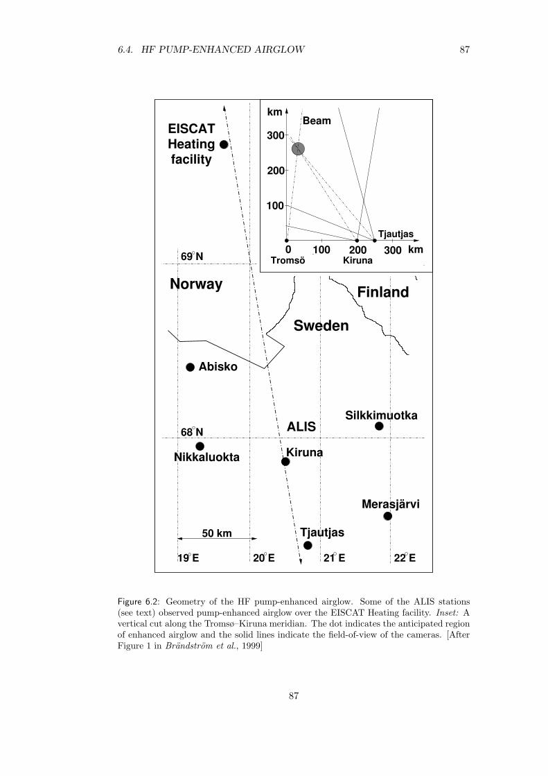
6.4. HF PUMP-ENHANCED AIRGLOW 87
EISCATHeatingfacility
19 E 20 E 21 E 22 E
69 N
68 N
Norway
Sweden
Finland
ALIS
Nikkaluokta
Abisko
Kiruna
Silkkimuotka
Merasjärvi
Tjautjas50 km
100 300
100
200Tromsö
0Kiruna
Tjautjas
km
300
200
kmBeam
Figure 6.2: Geometry of the HF pump-enhanced airglow. Some of the ALIS stations(see text) observed pump-enhanced airglow over the EISCAT Heating facility. Inset: Avertical cut along the Tromsø–Kiruna meridian. The dot indicates the anticipated regionof enhanced airglow and the solid lines indicate the field-of-view of the cameras. [AfterFigure 1 in Brandstrom et al., 1999]
87
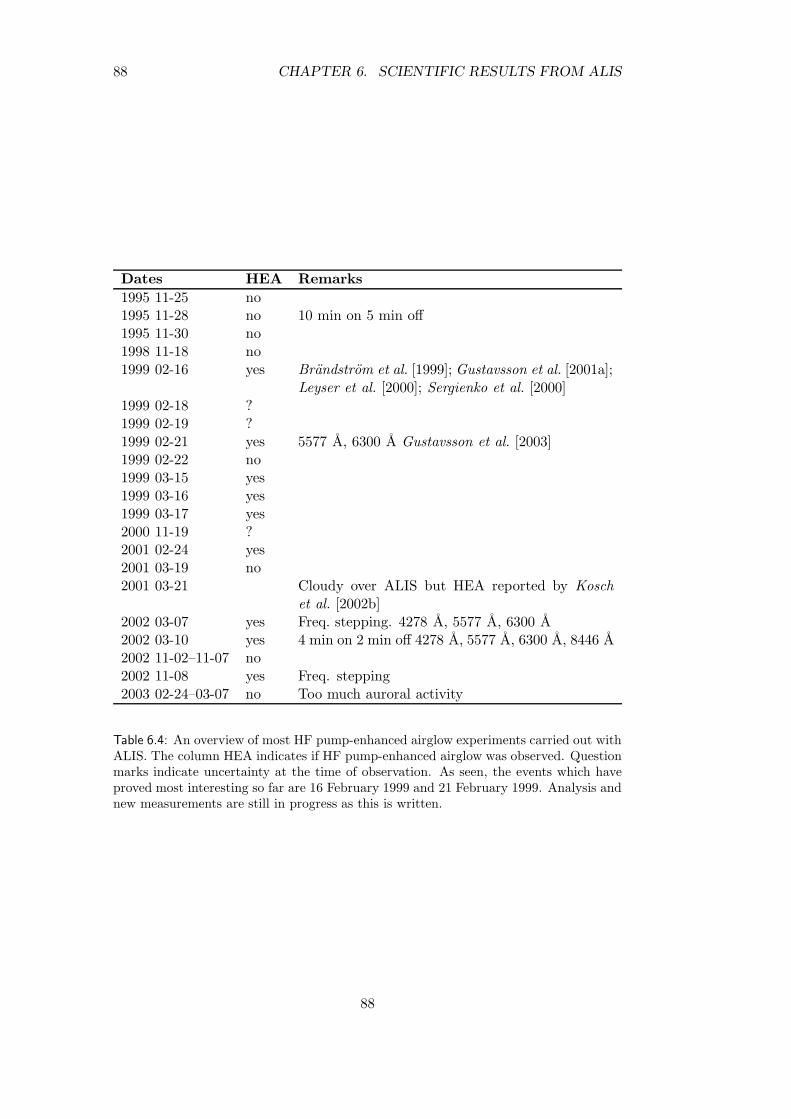
88 CHAPTER 6. SCIENTIFIC RESULTS FROM ALIS
Dates HEA Remarks
1995 11-25 no1995 11-28 no 10 min on 5 min off1995 11-30 no1998 11-18 no1999 02-16 yes Brandstrom et al. [1999]; Gustavsson et al. [2001a];
Leyser et al. [2000]; Sergienko et al. [2000]1999 02-18 ?1999 02-19 ?1999 02-21 yes 5577 A, 6300 A Gustavsson et al. [2003]1999 02-22 no1999 03-15 yes1999 03-16 yes1999 03-17 yes2000 11-19 ?2001 02-24 yes2001 03-19 no2001 03-21 Cloudy over ALIS but HEA reported by Kosch
et al. [2002b]2002 03-07 yes Freq. stepping. 4278 A, 5577 A, 6300 A2002 03-10 yes 4 min on 2 min off 4278 A, 5577 A, 6300 A, 8446 A2002 11-02–11-07 no2002 11-08 yes Freq. stepping2003 02-24–03-07 no Too much auroral activity
Table 6.4: An overview of most HF pump-enhanced airglow experiments carried out withALIS. The column HEA indicates if HF pump-enhanced airglow was observed. Questionmarks indicate uncertainty at the time of observation. As seen, the events which haveproved most interesting so far are 16 February 1999 and 21 February 1999. Analysis andnew measurements are still in progress as this is written.
88

6.4. HF PUMP-ENHANCED AIRGLOW 89
1000
1500
2000mean intensitymax intensity heater on
1000
2000
3000
1000
2000
3000
4000
1650 1700 1710 1720 1730 1740 1750 1800 1810 1820 18301000
1500
2000
PSfrag replacements
Kiruna
Abisko
Silkkimuotka
Nikkaluokta
time (UT)
Cou
nts
Cou
nts
Cou
nts
Cou
nts
Figure 6.3: Maximum and average column emission of the 6300 A airglow as seen fromfour stations. The intensity modulations correlate well with the transmitter-on/off cycles.After 17:40 UTC the Kiruna camera was directed to local zenith, imaging the naturalbackground airglow. [After Figure 1 in Gustavsson et al., 2001a]
in the ionospheric F-region above the transmitters). The transmitters (or “HF-pump”) were cycled on/off with a duty cycle of 50%. Between 16:32 and 17:22UTC the transmitters were cycled 2 min on/2 min off. Between 17:24 and 18:32UTC this was changed to 4 min on/4 min off.
When the transmitters were cycled 2 min on/2 min off, weak airglow enhance-ments were observed [Brandstrom et al., 1999; Leyser et al., 2000; Gustavssonet al., 2001a]. Starting at 17:32 UTC and continuing until 18:30 UTC (trans-mitters 4 min on/4 min off) pump-enhanced airglow was observed by all ALISstations in operation. Due to occasional thin clouds and technical problems, somedata-losses occurred. In Figure 6.3 the maximum intensity of the 6300 A emissionis plotted against time for each image from the four stations observing between16:40 and 18:40 UTC.
The airglow intensity has an e-folding growth time of about 60 s aftertransmitter-on, and decays with an e-folding decay time of about 35 s aftertransmitter-off. After the growth time following transmitter-on, the maximumintensity of the emission appears to have a different temporal evolution at differ-ent transmitter-on/off periods. This feature may be due to irregularities in the
89

90 CHAPTER 6. SCIENTIFIC RESULTS FROM ALIS
17:40:15 17:40:35 17:40:55 17:41:15 17:41:35 17:41:55
0
1000
2000
3000
4000
17:43:55 17:44:05 17:44:15 17:44:25 17:44:35 17:44:45
0
1000
2000
3000
4000
Figure 6.4: Sequence of airglow images from the Silkkimuotka ALIS station for 20 sintervals following transmitter-on at 17:40:00 UTC (top), and at 10 s intervals followingtransmitter-off at 17:44:00 UTC (bottom). The intensity scale is in raw counts. Twopeaks of airglow intensification are clearly visible in the transmitter-on sequence. [AfterFigure 3 in Brandstrom et al., 1999]
background ionosphere, which drift through the transmitted beam.
A series of images of the airglow intensity is shown in Figure 6.4. Transmitter-on occurs at 17:40 UTC, beyond which the airglow region and intensity is seento slowly grow, forming two peaks. The upper one appears to saturate, afterwhich the lower peak underneath intensifies, and eventually merges with the firstpeak. Transmitter-off occurs at 17:44 UTC, beyond which the airglow slowlydecays. The peak intensity was estimated to be approximately 300± 100 R. (SeeSection 4.2.1, regarding the estimated error of the absolute calibration).
Figure 6.5 shows data from the Silkkimuotka station obtained neartransmitter-on at 17:48:00 UTC and -off at 17:52:00 UTC. Both the intensityand size of the patch are seen to slowly increase after transmitter-on, and todecay slowly after transmitter-off.
From Figure 6.3 it is seen that simultaneous data from up to three stationsexist for some time periods. This enables triangulation of the height of theairglow region. As shown in the top panel in Figure 6.6, the typical heightof the maximum emission was found to be 230–240 km from 17:32 UTC to18:08 UTC. For the transmitter-on at 18:12 UTC, the enhanced airglow alti-tude is 250-260 km. In the bottom panel it is shown that the airglow region waspositioned approximately 160–170 km to the north of Kiruna and 50 km to thewest.
In Figure 6.7, it is seen that the initial location of the two interaction regionsare approximately 20–30 km apart. The initially more intensive northernmostregion of excitation is fairly immobile, while the southernmost moves 30 kmnorthward in 4 minutes corresponding to a velocity of 100 ± 20 m/s [Gustavssonet al., 2001a].
Also, the ionospheric F-region neutral wind was measured by Fabry-Perotinterferometers (FPI) [Aruliah et al., 1996; Gustavsson et al., 2001a]. Figure 6.8
90
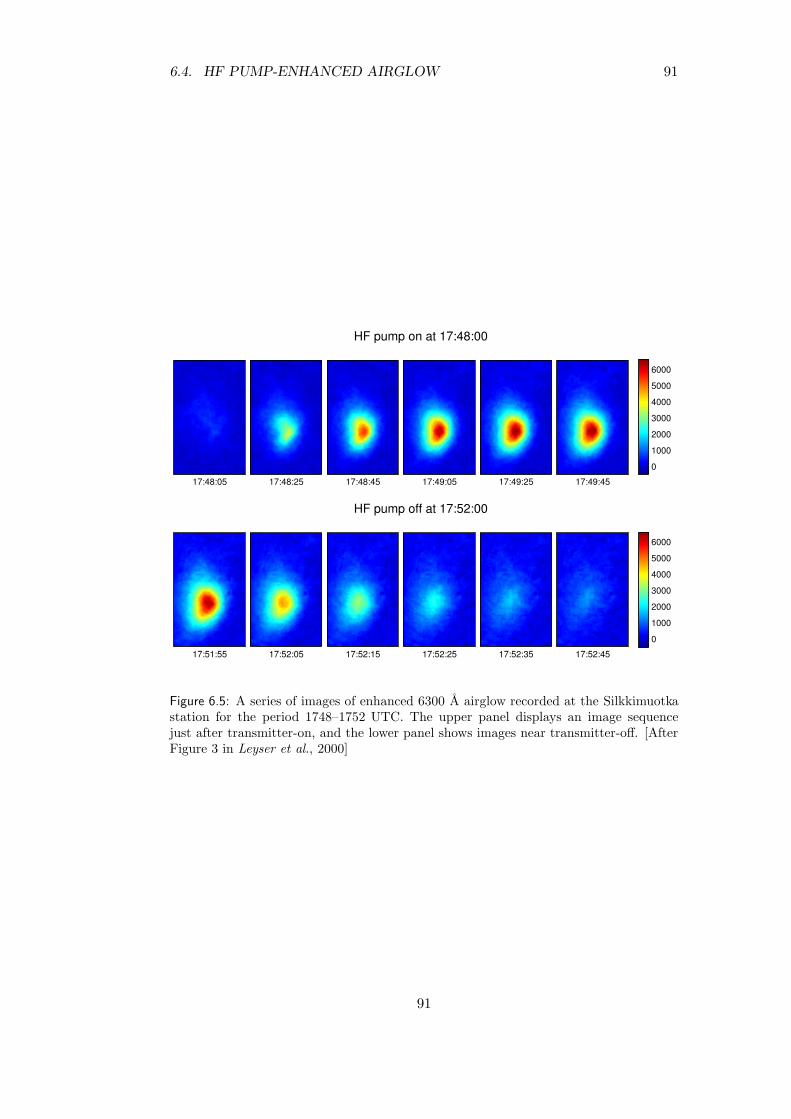
6.4. HF PUMP-ENHANCED AIRGLOW 91
17:48:05 17:48:25 17:49:05 17:49:25 17:49:45
0
1000
2000
3000
4000
5000
6000
17:51:55 17:52:05 17:52:25 17:52:35 17:52:45
0
1000
2000
3000
4000
5000
6000
17:48:45
HF pump on at 17:48:00
17:52:15
HF pump off at 17:52:00
Figure 6.5: A series of images of enhanced 6300 A airglow recorded at the Silkkimuotkastation for the period 1748–1752 UTC. The upper panel displays an image sequencejust after transmitter-on, and the lower panel shows images near transmitter-off. [AfterFigure 3 in Leyser et al., 2000]
91
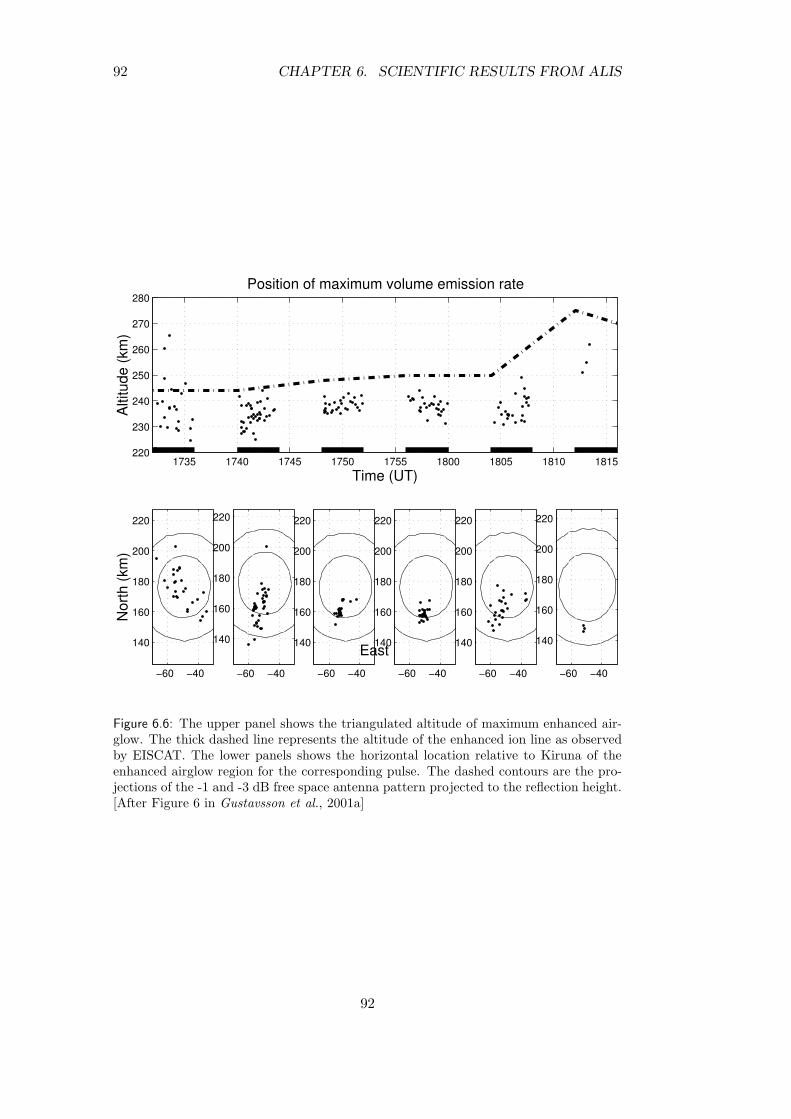
92 CHAPTER 6. SCIENTIFIC RESULTS FROM ALIS
1735 1740 1745 1750 1755 1800 1805 1810 1815220
230
240
250
260
270
280
Time (UT)
Position of maximum volume emission rate
Alti
tude
(km
)
−60 −40
140
160
180
200
220
Nor
th (k
m)
−60 −40
140
160
180
200
220
−60 −40
140
160
180
200
220
East (km)−60 −40
140
160
180
200
220
−60 −40
140
160
180
200
220
−60 −40
140
160
180
200
220
Figure 6.6: The upper panel shows the triangulated altitude of maximum enhanced air-glow. The thick dashed line represents the altitude of the enhanced ion line as observedby EISCAT. The lower panels shows the horizontal location relative to Kiruna of theenhanced airglow region for the corresponding pulse. The dashed contours are the pro-jections of the -1 and -3 dB free space antenna pattern projected to the reflection height.[After Figure 6 in Gustavsson et al., 2001a]
92
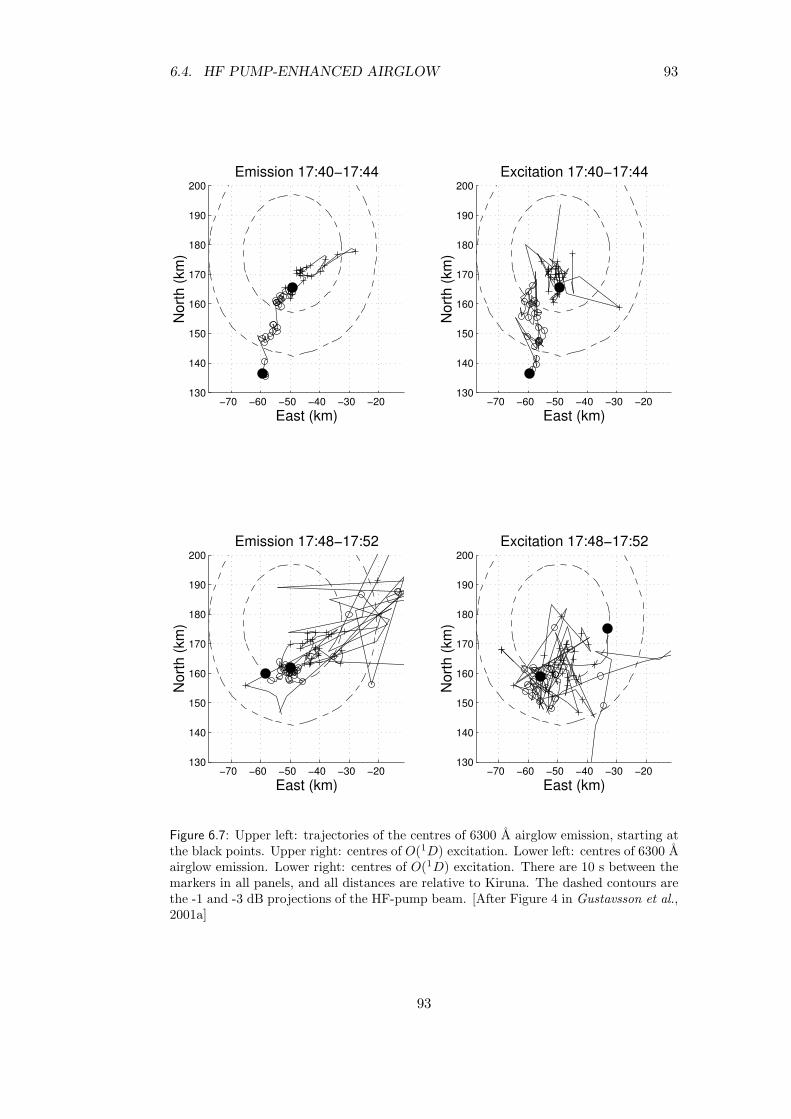
6.4. HF PUMP-ENHANCED AIRGLOW 93
−70 −60 −50 −40 −30 −20130
140
150
160
170
180
190
200Emission 17:40−17:44
East (km)
Nor
th (k
m)
−70 −60 −50 −40 −30 −20130
140
150
160
170
180
190
200Excitation 17:40−17:44
East (km)
Nor
th (k
m)
−70 −60 −50 −40 −30 −20130
140
150
160
170
180
190
200Emission 17:48−17:52
East (km)
Nor
th (k
m)
−70 −60 −50 −40 −30 −20130
140
150
160
170
180
190
200Excitation 17:48−17:52
East (km)
Nor
th (k
m)
Figure 6.7: Upper left: trajectories of the centres of 6300 A airglow emission, starting atthe black points. Upper right: centres of O(1D) excitation. Lower left: centres of 6300 Aairglow emission. Lower right: centres of O(1D) excitation. There are 10 s between themarkers in all panels, and all distances are relative to Kiruna. The dashed contours arethe -1 and -3 dB projections of the HF-pump beam. [After Figure 4 in Gustavsson et al.,2001a]
93
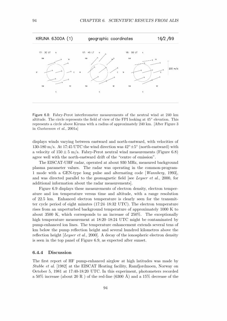
94 CHAPTER 6. SCIENTIFIC RESULTS FROM ALIS
Figure 6.8: Fabry-Perot interferometer measurements of the neutral wind at 240 kmaltitude. The circle represents the field of view of the FPI looking at 45 elevation. Thisrepresents a circle above Kiruna with a radius of approximately 240 km. [After Figure 3in Gustavsson et al., 2001a]
displays winds varying between eastward and north-eastward, with velocities of130-180 m/s. At 17:45 UTC the wind direction was 42±5 (north-eastward) witha velocity of 150 ± 5 m/s. Fabry-Perot neutral wind measurements (Figure 6.8)agree well with the north-eastward drift of the “centre of emission”.
The EISCAT-UHF radar, operated at about 930 MHz, measured backgroundplasma parameter values. The radar was operating in the common-program-1 mode with a GEN-type long pulse and alternating code [Wannberg , 1993],and was directed parallel to the geomagnetic field [see Leyser et al., 2000, foradditional information about the radar measurements].
Figure 6.9 displays these measurements of electron density, electron temper-ature and ion temperature versus time and altitude, with a range resolutionof 22.5 km. Enhanced electron temperature is clearly seen for the transmit-ter cycle period of eight minutes (17:24–18:32 UTC). The electron temperaturerises from an unperturbed background temperature of approximately 1000 K toabout 3500 K, which corresponds to an increase of 250%. The exceptionallyhigh temperature measurement at 18:20–18:24 UTC might be contaminated bypump-enhanced ion lines. The temperature enhancement extends several tens ofkm below the pump reflection height and several hundred kilometres above thereflection height [Leyser et al., 2000]. A decay of the ionospheric electron densityis seen in the top panel of Figure 6.9, as expected after sunset.
6.4.4 Discussion
The first report of HF pump-enhanced airglow at high latitudes was made byStubbe et al. [1982] at the EISCAT Heating facility, Ramfjordmoen, Norway onOctober 5, 1981 at 17:40-18:20 UTC. In this experiment, photometers recordeda 50% increase (about 20 R ) of the red-line (6300 A) and a 15% decrease of the
94
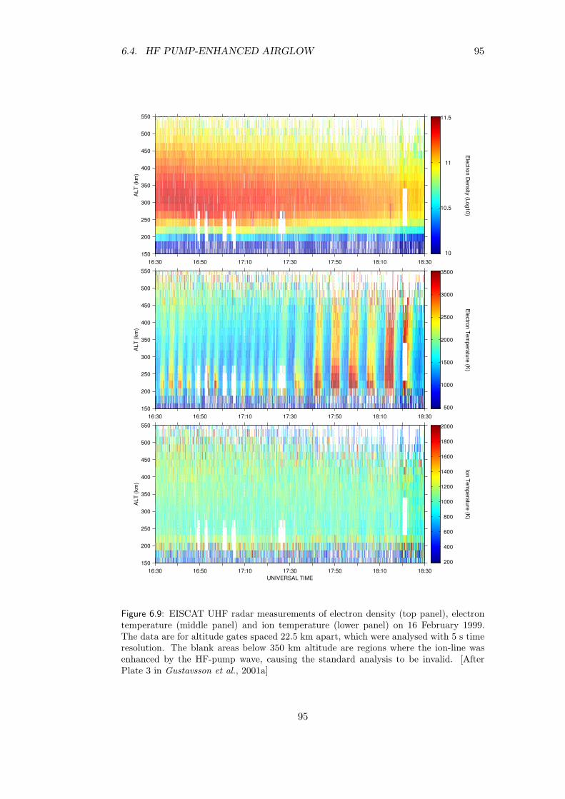
6.4. HF PUMP-ENHANCED AIRGLOW 95
16:30 16:50 17:10 17:30 17:50 18:10 18:30150
200
250
300
350
400
450
500
550
Electron D
ensity (Log10)
ALT
(km
)
10
10.5
11
11.5
16:30 16:50 17:10 17:30 17:50 18:10 18:30150
200
250
300
350
400
450
500
550
Electron Tem
perature (K)
ALT
(km
)
500
1000
1500
2000
2500
3000
3500
16:30 16:50 17:10 17:30 17:50 18:10 18:30150
200
250
300
350
400
450
500
550
Ion Temperature (K
)
UNIVERSAL TIME
ALT
(km
)
200
400
600
800
1000
1200
1400
1600
1800
2000
Figure 6.9: EISCAT UHF radar measurements of electron density (top panel), electrontemperature (middle panel) and ion temperature (lower panel) on 16 February 1999.The data are for altitude gates spaced 22.5 km apart, which were analysed with 5 s timeresolution. The blank areas below 350 km altitude are regions where the ion-line wasenhanced by the HF-pump wave, causing the standard analysis to be invalid. [AfterPlate 3 in Gustavsson et al., 2001a]
95
96 CHAPTER 6. SCIENTIFIC RESULTS FROM ALIS
green line (5577 A) during transmitter-on periods. The frequency was 5.423 MHz,and an O-mode beam with an ERP of 260 MW was switched 5 min on/5 minoff. However, simultaneous observations made by Henriksen et al. [1984] didnot find any evidence of pump enhanced airglow, which casted some doubts onthe results by Stubbe et al. [1982]. In both of these observations, the opticalinstrumentation was scanning photometers with field-of-view of about 5. Thiscould have introduced aiming problems, causing the photometers to measure inthe wrong region of the sky. On the other hand, it must be noted that RadioFrequency Interference (RFI) is more likely to produce false positive results froma photometer, as compared with an imager as a shift of bias of a single readoutchannel is more likely to be affected than all pixels in an image. These remarksillustrate why multi-station imaging measurements are superior to photometersgiven enough sensitivity. Such cameras were not available at the time of theexperiments cited above.
The first clearly unambiguous observations of high-latitude HF pump-enhanced airglow were made on 16 February 1999, as described in the previ-ous section. The positive result of this and subsequent observations might beattributed to some of the following reasons: improved optical instrumentation,more favourable ionospheric conditions, the approaching solar maximum. Whilethe previous positive observation by Stubbe et al. [1982], relied on photometermeasurements made from the same site as the EISCAT Heating facility, theresults from 16 February 1999 were obtained by several stations located about150–200 km away from the heating facility. Therefore, direct RFI from the trans-mitters can be clearly ruled out for these observations. The observations havealso been confirmed by simultaneous measurements from an independent imager[Kosch et al., 2000b,a, 2002b] on several occasions. It could therefore be statedthat the validity of these observations are beyond all reasonable doubt. In addi-tion, HF pump-enhanced airglow was observed at auroral latitudes at the HighFrequency Active Auroral Research Program facility (HAARP) facility in Alaska[Pedersen and Carlson, 2001].
In Brandstrom et al. [1999] the observations of 16 February 1999 are foundto be similar to the observations by Bernhardt et al. [1991] where an 165 MW,5.828 MHz O-mode beam produced ≥ 200 R of airglow near zenith above theSURA-facility (latitude 56N) in Russia.
The two intensity peaks in Figure 6.4, resemble seed irregularities as discussedby Bernhardt et al. [1991]. The drift-pattern of the two intensity peaks (Fig-ure 6.7) is probably associated with electric fields and neutral-wind convection.During the next transmitter-on period 17:48–17:52 UTC, (Figure 6.5) a singlepatch of enhanced airglow appeared. Leyser et al. [2000] attributes this vari-ability to possible large-scale plasma density irregularities in the pump-plasmainteraction region.
The altitude of maximum volume emission is slightly lower than the pumpreflection height of approximately 250 km as measured with the Dynasonde andEISCAT-UHF radar. These measurements are consistent with model calculationsof the airglow emission altitude for different source altitudes of monoenergeticelectrons [Bernhardt et al., 1989].
The observed decay time of the airglow of approximately 30–35 s is signi-
96
6.4. HF PUMP-ENHANCED AIRGLOW 97
ficantly shorter than the 110 s lifetime of the O(1D) metastable state [Solomonet al., 1988]. However, at 240 km altitude, the effective life time of the O(1D)emission is reduced due to collisional quenching by excitation of vibrational statesin N2 and O2 to as low values as 30 s [Sipler and Biondi , 1972; Bernhardt et al.,1991]. Thus, the observed decay time is consistent with the effective life time ofthe O(1D) state being reduced by quenching [Leyser et al., 2000].
Sergienko et al. [2000] used EISCAT measurements of the electron temperat-ure to estimate the position and magnitude of the heating source. The magnitudeof a modelled electron heating source was adjusted to give the best fit to the ob-served time-behaviour of the electron temperatures at all altitudes. This proced-ure led to a determination of the position and magnitude of the electron-heatingsource at 220 km altitude and 6 × 10⁴ eVs−1 cm−3 respectively. A good agree-ment with the measured and calculated electron temperatures were obtained.The next step was to compare modelled and measured column emission ratesof the O(1D) (6300 A) line. Assuming a thermal excitation mechanism led tolarge overestimates of the modelled column emission rates as compared to anaccelerated electron excitation mechanism. The paper shows that the assump-tion of abnormal electron heating generated by the transmitted wave leads to apossible explanation of the observed electron-temperature variations, but cannotaccount for the observed airglow variations. A process resembling acceleration byLangmuir turbulence (where the electrons above 2 eV are non-Maxwellian with auniform energy distribution from 3–10 eV) might be an alternative explanationfor airglow enhancements. This modelling was done according to the analysis byBernhardt et al. [1989] and by calculating the production rate of the O(1D) stateby electron impact according to the Monte Carlo model for electron transportinto the atmosphere by Ivanov and Sergienko [1992].
It was, however, later found out that the electrons are more likely acceleratedby upper hybrid turbulence [see Leyser et al., 2000] instead of Langmuir turbu-lence. For example, if the pump-frequency is close to a multiple of the electrongyro-frequency, the optical emissions in 6300 A and 5577 A becomes very faint[Kosch et al., 2002a] while the Langmuir turbulence is very strong. This is alsoconsistent with results from tomographic inversion, which resulted in a too lowaltitude for Langmuir-turbulence. [Leyser and Gustavsson, 2003]
The most complete treatment of the observations from 16 February 1999(so far) is presented in Gustavsson et al. [2001a]. This paper presents the firstestimate of the volume distribution the HF pump-enhanced airglow emissionobtained from a tomography-like analysis of the image data. Where data fromthree stations exists (17:40–17:56 UTC), the tomography-like inversion proceduregives reliable results [see Gustavsson et al., 2001a, for details]. For periods withdata from only two stations a stereoscopic triangulation method was employed todetermine the position of the enhanced airglow region. In Figure 6.10 the resultof the tomography-like inversion is presented. The shape of the excitation variesfrom prolate along the magnetic field to slightly oblate. Also, the existence oftwo separable regions is clearly seen in the figure. These results were validatedby back-projecting images from the reconstructed volume and comparing themto the original images. Comparing the images [see Gustavsson et al., 2001a] givesa typical maximum error of ±10%. Thin drifting clouds in Abisko as well as
97
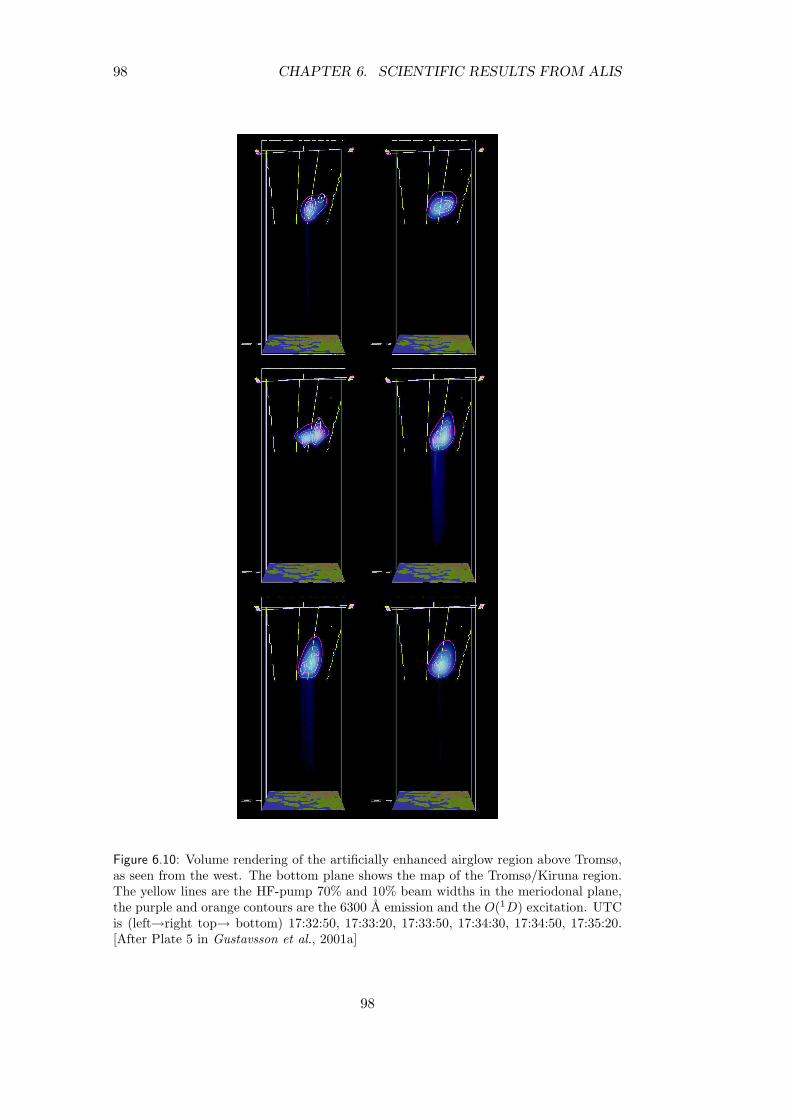
98 CHAPTER 6. SCIENTIFIC RESULTS FROM ALIS
Figure 6.10: Volume rendering of the artificially enhanced airglow region above Tromsø,as seen from the west. The bottom plane shows the map of the Tromsø/Kiruna region.The yellow lines are the HF-pump 70% and 10% beam widths in the meriodonal plane,the purple and orange contours are the 6300 A emission and the O(1D) excitation. UTCis (left→right top→ bottom) 17:32:50, 17:33:20, 17:33:50, 17:34:30, 17:34:50, 17:35:20.[After Plate 5 in Gustavsson et al., 2001a]
98
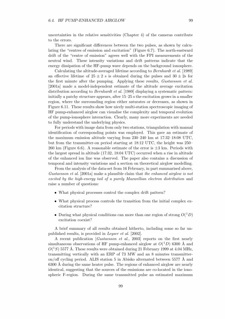
6.4. HF PUMP-ENHANCED AIRGLOW 99
uncertainties in the relative sensitivities (Chapter 4) of the cameras contributeto the errors.
There are significant differences between the two pulses, as shown by calcu-lating the “centres of emission and excitation” (Figure 6.7). The north-eastwarddrift of the “centre of emission” agrees well with the FPI measurements of theneutral wind. These intensity variations and drift patterns indicate that theenergy dissipation of the HF-pump wave depends on the background ionosphere.
Calculating the altitude-averaged lifetime according to Bernhardt et al. [1989]an effective lifetime of 25 ± 2 s is obtained during the pulses and 30 ± 2s forthe first minute after the pumping. Applying these results, Gustavsson et al.[2001a] made a model-independent estimate of the altitude average excitationdistribution according to Bernhardt et al. [1989] displaying a systematic pattern:initially a patchy structure appears, after 15–25 s the excitation grows in a smallerregion, where the surrounding region either saturates or decreases, as shown inFigure 6.11. These results show how nicely multi-station spectroscopic imaging ofHF pump-enhanced airglow can visualise the complexity and temporal evolutionof the pump-ionosphere interaction. Clearly, many more experiments are neededto fully understand the underlying physics.
For periods with image data from only two stations, triangulation with manualidentification of corresponding points was employed. This gave an estimate ofthe maximum emission altitude varying from 230–240 km at 17:32–18:08 UTC,but from the transmitter-on period starting at 18:12 UTC, the height was 250–260 km (Figure 6.6). A reasonable estimate of the error is ±3 km. Periods withthe largest spread in altitude (17:32, 18:04 UTC) occurred when a rise in altitudeof the enhanced ion line was observed. The paper also contains a discussion oftemporal and intensity variations and a section on theoretical airglow modelling.
From the analysis of the data-set from 16 February, in part summarised above,Gustavsson et al. [2001a] make a plausible claim that the enhanced airglow is notexcited by the high-energy tail of a purely Maxwellian electron distribution andraise a number of questions:
• What physical processes control the complex drift pattern?
• What physical process controls the transition from the initial complex ex-citation structure?
• During what physical conditions can more than one region of strong O(1D)excitation coexist?
A brief summary of all results obtained hitherto, including some so far un-published results, is provided in Leyser et al. [2002].
A recent publication [Gustavsson et al., 2003] reports on the first nearlysimultaneous observations of HF pump-enhanced airglow at O(1D) 6300 A andO(1S) 5577 A. These results were obtained during 21 February 1999 at 4.04 MHz,transmitting vertically with an ERP of 73 MW and an 8 minutes transmitter-on/off cycling period. ALIS station 5 in Abisko alternated between 5577 A and6300 A during the same heater pulse. The regions of enhanced airglow are nearlyidentical, suggesting that the sources of the emissions are co-located in the iono-spheric F-region. During the same transmitted pulse an estimated maximum
99
100 CHAPTER 6. SCIENTIFIC RESULTS FROM ALIS
17:39:55
Cou
nts
17:40:05 17:40:15 17:40:25 17:40:35
1000
2000
3000
17:31:55
Cou
nts
17:32:05 17:32:15 17:32:25 17:32:35
1000
2000
3000
17:47:55
Cou
nts
17:48:05 17:48:15 17:48:25 17:48:35
1000
2000
3000
17:55:55
Cou
nts
17:56:05 17:56:15 17:56:25 17:56:35
1000
2000
3000
18:03:55
Cou
nts
18:04:05 18:04:15 18:04:25 18:04:35
1000
2000
3000
Figure 6.11: Estimates of the O(1D) excitation rates for the period just beforetransmitter-on and the four 10 s periods just after transmitter-on for five pulses. Thearrows are the neutral wind direction projected to the images. All images are from theALIS station in Silkkimuotka. [After Plate 7 in Gustavsson et al., 2001a]
100
6.5. AURORAL STUDIES 101
column emission rate of about 40–60 Rayleighs in 6300 A and with a maximumcolumn emission rate of about 10–20 Rayleighs in 5577 A were observed. Thesepreliminary results indicate that an intensity-ratio of 5577 A and 6300 A of about0.3–0.4 implies that the excitation is caused by a non-thermal electron population.Previously obtained intensity ratios were 0.05–0.3 [Haslett and Megill , 1974], and0.08 [Bernhardt et al., 1989].
HF pump-enhanced airglow in the N+2 1Neg. 4278 A emission was observed in
photometer data from 2001 by Kaila [2003b]. In March 2002 ALIS observed HFpump-enhanced airglow in N+
2 1Neg. 4278 A. In this experiment the transmittedwave was stepped up and down in frequency through the third harmonic of theionospheric electron gyro frequency. The airglow was simultaneously imagedwith one CCD camera operated at 6300 A by M. Kosch in Skibotn, and themobile ALIS station (Section A.8) located at the same place. The ALIS camerarecorded emissions in 5577 A as the frequency was stepped downward throughthe gyro harmonic, and weaker 4278 A emissions as the transmitted frequencywas stepped up again. This is the first time that pump-enhanced ionisationof the thermosphere has been directly observed. Furthermore, the frequencydependence of the 4278 A emission gives input to theoretical modelling of electronacceleration for HF-frequencies near the harmonics. It is important in futureexperiments to be able to reconstruct the volume distribution of the N +
2 1Neg.emission and compare with the volume distribution of for example O(1D) tostudy the role of the underlying plasma dynamics perpendicular and parallel tothe geomagnetic field [Leyser et al., 2002]. Therefore it is essential to obtain moremulti-station measurements with ALIS in the future.
6.5 Auroral studies
Although ALIS was built for auroral observations, and consequently most ofits observing time was spent on auroral observations, the amount of publishedscientific results in this field have been sparse. One explanation is that oncethe HF pump-enhanced airglow experiments proved successful, it was deemed farmore productive for a small group to spend time publishing these results. Othercontributing factors are the technical problems affecting the maximum framerate(Section 3.3.4). Furthermore, as ALIS is a new type of instrument, much remainsto be learned about how to exploit it in the optimal way. The amount of datais also somewhat limited as auroral studies often are dependent on a variety ofcoordinated observations with other instruments.
When planning coordinated studies with satellites as well as ground-basedradars and optical instruments, many criteria need to be fulfilled; near new-moon, clear skies, the satellite magnetic footprint needs to be reasonably closeto the ground-based instruments, radar observing-time needs to be applied forand scheduled [Hedin et al., 1999]. Furthermore, the probability of observingthe desired auroral phenomena must be maximised for the ground-based sitestaking part in the study. For campaigns involving satellite passes, slow magneticmidnight passes are optimal. Yet, fulfilling all of these criteria for a successfulobservation might take a very long time. Therefore patience, long-term stabilityand flexibility in changing the scientific objectives are key-issues. An auroral
101
102 CHAPTER 6. SCIENTIFIC RESULTS FROM ALIS
event cannot be made to occur at the desired time or place to fit a particularmeasurement. However, well-planned observations will increase the probability ofmaking useful observations. In this section some of the results related to auroralstudies are summarised.
6.5.1 An estimate of the auroral electron spectra
One of the traditional emission lines of choice for monochromatic auroral imagingis the O(1D) 6300 A emission line [Solomon et al., 1988; Meier et al., 1989].However, the excitation mechanism of that line is still under some debate [Meieret al., 1989]. As the excited O(1D) state is quenched at lower altitudes, theratios of the column emission rates for the O(1D) 6300 A and N+
2 1Neg. 4278 Aemission-lines have been taken as an indicator of the characteristic energies of theprecipitating electrons. The long radiative lifetime of the O(1D) 6300 A emissionline makes comparisons with the rapid N+
2 1Neg. 4278 A and O(1S) 5577 Aemission-lines difficult, particularly for active auroral events.
In 1996 the first ALIS station was equipped with filters for the O(3p3P ) 8446 Aemission line. Initial observations confirmed a sufficient signal strength for theALIS-Imagers, and subsequently all stations were equipped with filters for thisemission-line.
A preliminary study [Steen et al., 1999a] presents data from 25 March 1998.Two ALIS stations (Kiruna and Merasjarvi) provided data from an auroral eventoccurring at the end of a geomagnetically disturbed period. An eastward travel-ling fold similar to that described by Steen et al. [1988] first appeared in the westand traversed the Kiruna zenith at about 1000 m/s as estimated from all-skyimages. After that, the arc broke up and was replaced by a diffuse auroral band.The fold was observed in O(1D) 6300 A, O(1S) 5577 A, N+
2 1Neg. 4278 A, andO(3p3P ) 8446 A. The observed fold appeared almost identical in all emission-lines, except, as expected in the slow O(1D) emission. This initial study con-cluded that the O(3p3P ) 8446 A auroral morphology appears similar to that ofN+
2 1Neg. 4278 A.In a more extensive study [Gustavsson et al., 2001b], two methods for es-
timating characteristics of primary electron spectra are compared and used todescribe the auroral event of 25 March 1998. One method uses the spectralinformation in the images (Figure 6.12), while the other method is based onan inversion of the N+
2 1Neg. 4278 A altitude distribution. Using the secondmethod, ALIS can currently give estimates of the primary electron distributionwith a time resolution of about 10 s (Figure 6.13). The paper concludes thatonly two dimensional measurements are able to follow the dynamics of this typeof event, as single-point measurements cannot distinguish between temporal andspatial variations. Estimating the characteristic energy of precipitating electronsby combining measurements in 4278 A, 6300 A and 8446 A provides useful resultsfor temporal variations slower than 100 s. The primary electron spectra retrievedfrom the altitude distribution of the N+
2 1Neg. 4278 A emission can give estim-ates of the electron characteristics with 10 s time resolution, but only for discreteauroral structures. To fully exploit the information obtainable from these kind ofobservations requires a combination of spectral and spatial analysis and to com-pare the results with two-dimensional electron transport and ionospheric models.
102
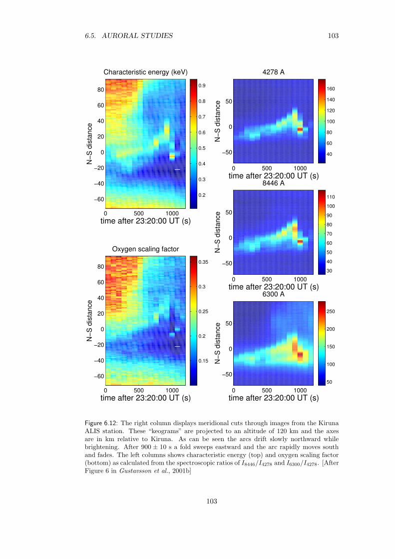
6.5. AURORAL STUDIES 103
0.2
0.3
0.4
0.5
0.6
0.7
0.8
0.9
0 500 1000
−60
−40
−20
0
20
40
60
80
time after 23:20:00 UT (s)
N−S
dis
tanc
e
Characteristic energy (keV)
0.15
0.2
0.25
0.3
0.35
0 500 1000
−60
−40
−20
0
20
40
60
80
time after 23:20:00 UT (s)
N−S
dis
tanc
e
Oxygen scaling factor
40
60
80
100
120
140
160
0 500 1000
−50
0
50
time after 23:20:00 UT (s)
N−S
dis
tanc
e
4278 A
30
40
50
60
70
80
90
100
110
0 500 1000
−50
0
50
time after 23:20:00 UT (s)
N−S
dis
tanc
e
8446 A
50
100
150
200
250
0 500 1000
−50
0
50
time after 23:20:00 UT (s)
N−S
dis
tanc
e
6300 A
Figure 6.12: The right column displays meridional cuts through images from the KirunaALIS station. These “keograms” are projected to an altitude of 120 km and the axesare in km relative to Kiruna. As can be seen the arcs drift slowly northward whilebrightening. After 900 ± 10 s a fold sweeps eastward and the arc rapidly moves southand fades. The left columns shows characteristic energy (top) and oxygen scaling factor(bottom) as calculated from the spectroscopic ratios of I8446/I4278 and I6300/I4278. [AfterFigure 6 in Gustavsson et al., 2001b]
103

104 CHAPTER 6. SCIENTIFIC RESULTS FROM ALIS
4.5
5
5.5
6
6.5
7
7.5
8
8.5
9
200 400 600 800 1000 1200
100
101
102
time after 23:20:00 UT (s)
elec
tron
ener
gy
log10
electron energy flux
Figure 6.13: An estimation of the energy flux by inversion of N+2 1Neg. 4278 A altitude
distribution. About 400 s after 23:20:00 UTC there appears to be a slight increase inboth total flux and typical energy. [After Figure 6 in Gustavsson et al., 2001b]
104
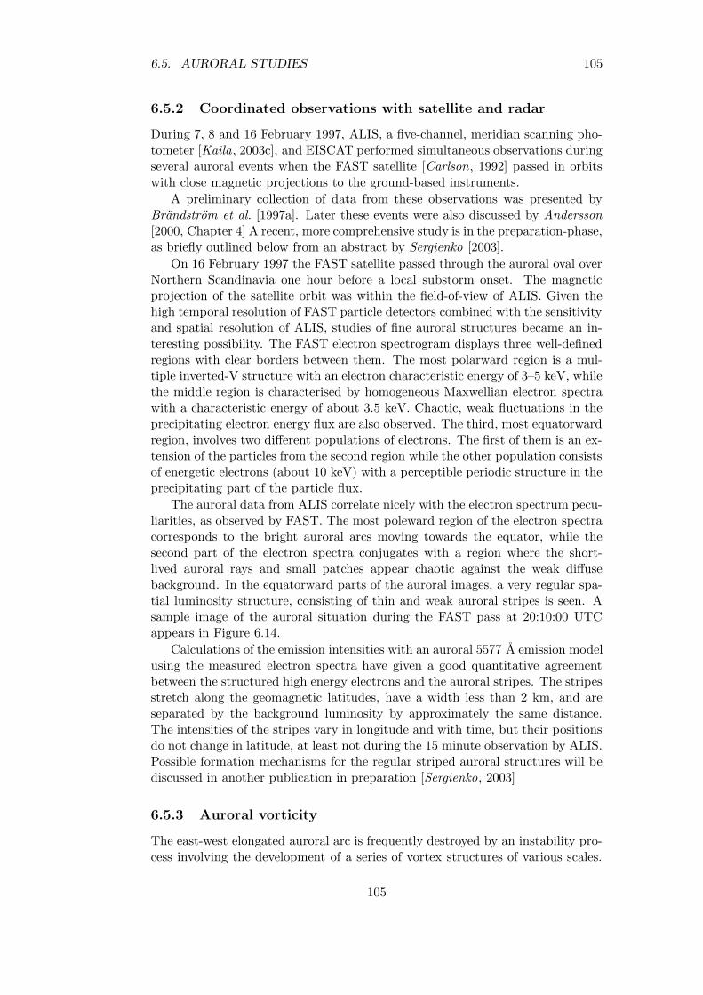
6.5. AURORAL STUDIES 105
6.5.2 Coordinated observations with satellite and radar
During 7, 8 and 16 February 1997, ALIS, a five-channel, meridian scanning pho-tometer [Kaila, 2003c], and EISCAT performed simultaneous observations duringseveral auroral events when the FAST satellite [Carlson, 1992] passed in orbitswith close magnetic projections to the ground-based instruments.
A preliminary collection of data from these observations was presented byBrandstrom et al. [1997a]. Later these events were also discussed by Andersson[2000, Chapter 4] A recent, more comprehensive study is in the preparation-phase,as briefly outlined below from an abstract by Sergienko [2003].
On 16 February 1997 the FAST satellite passed through the auroral oval overNorthern Scandinavia one hour before a local substorm onset. The magneticprojection of the satellite orbit was within the field-of-view of ALIS. Given thehigh temporal resolution of FAST particle detectors combined with the sensitivityand spatial resolution of ALIS, studies of fine auroral structures became an in-teresting possibility. The FAST electron spectrogram displays three well-definedregions with clear borders between them. The most polarward region is a mul-tiple inverted-V structure with an electron characteristic energy of 3–5 keV, whilethe middle region is characterised by homogeneous Maxwellian electron spectrawith a characteristic energy of about 3.5 keV. Chaotic, weak fluctuations in theprecipitating electron energy flux are also observed. The third, most equatorwardregion, involves two different populations of electrons. The first of them is an ex-tension of the particles from the second region while the other population consistsof energetic electrons (about 10 keV) with a perceptible periodic structure in theprecipitating part of the particle flux.
The auroral data from ALIS correlate nicely with the electron spectrum pecu-liarities, as observed by FAST. The most poleward region of the electron spectracorresponds to the bright auroral arcs moving towards the equator, while thesecond part of the electron spectra conjugates with a region where the short-lived auroral rays and small patches appear chaotic against the weak diffusebackground. In the equatorward parts of the auroral images, a very regular spa-tial luminosity structure, consisting of thin and weak auroral stripes is seen. Asample image of the auroral situation during the FAST pass at 20:10:00 UTCappears in Figure 6.14.
Calculations of the emission intensities with an auroral 5577 A emission modelusing the measured electron spectra have given a good quantitative agreementbetween the structured high energy electrons and the auroral stripes. The stripesstretch along the geomagnetic latitudes, have a width less than 2 km, and areseparated by the background luminosity by approximately the same distance.The intensities of the stripes vary in longitude and with time, but their positionsdo not change in latitude, at least not during the 15 minute observation by ALIS.Possible formation mechanisms for the regular striped auroral structures will bediscussed in another publication in preparation [Sergienko, 2003]
6.5.3 Auroral vorticity
The east-west elongated auroral arc is frequently destroyed by an instability pro-cess involving the development of a series of vortex structures of various scales.
105
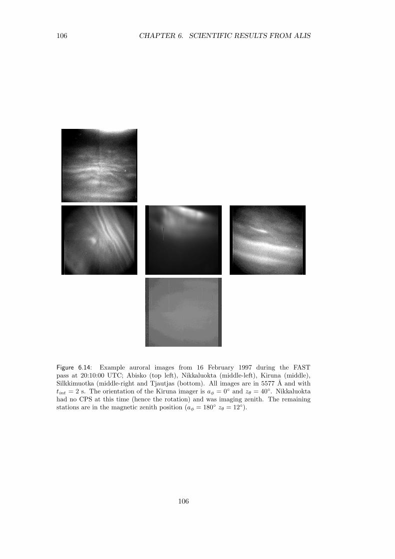
106 CHAPTER 6. SCIENTIFIC RESULTS FROM ALIS
Figure 6.14: Example auroral images from 16 February 1997 during the FASTpass at 20:10:00 UTC; Abisko (top left), Nikkaluokta (middle-left), Kiruna (middle),Silkkimuotka (middle-right and Tjautjas (bottom). All images are in 5577 A and withtint = 2 s. The orientation of the Kiruna imager is aφ = 0 and zθ = 40. Nikkaluoktahad no CPS at this time (hence the rotation) and was imaging zenith. The remainingstations are in the magnetic zenith position (aφ = 180 zθ = 12).
106

6.5. AURORAL STUDIES 107
Vorticity, ζ, is the measure of rotation in a fluid, ζ = ∇ × u (where u is thefluid velocity). Pudovkin et al. [1997] published a theoretical and experimentalreview of data connected with vorticity in the magnetospheric plasma and on itssignatures in the auroral dynamics. Early ALIS images were used in this paperto exemplify what can be learned from studying vortex structures in the aurora.Such studies can yield an abundant information on the physical state of the mag-netospheric plasma as well as the processes developing in it. For example, byobserving auroral forms with high temporal and spatial resolution, it is possibleto determine the distribution of the electric field and field-aligned currents in themagnetosphere. The shape of auroral vortices, carry information on the nature ofthe Magnetohydrodynamical (MHD) instabilities responsible for the excitation ofthe observed turbulence. Subsequent experimental work by for example Trond-sen [1998, and references therein] is an excellent example of research in this field.Due to technical problems affecting the maximum achievable temporal resolution(Section 3.3.4), ALIS has not been perfectly suited to continue studies in thisfield.
6.5.4 Studies of the ionospheric trough
An example showing that ALIS sometimes can provide usable supporting meas-urements, even when not operated in a scientific mode is presented by Hedinet al. [1999, 2000]. In this study of the main ionospheric trough, all the EISCATradars were for the first time operated in a four-beam configuration close to themeridian plane in order to obtain a wide area of observation without the lossof temporal resolution [Hedin et al., 2000]. This combined “meta-radar” has ahuge fan-like observation area, of about 70N–80N in geographic latitude [Hedinet al., 2000]. Supporting measurements were provided by the FAST satellite andALIS. During the night of 14 March 1997, ALIS was only operated occasion-ally since there were no significant aurora, and the conditions at some stationswere partly cloudy. The images were obtained randomly in order to check cloudconditions etc. However, some images happened to be acquired at relevant timesfor the trough study, displaying faint, diffuse auroral structures around the timewhen the trough poleward boundary passed over the field-of-view of ALIS. Theposition of the diffuse aurora obtained from ALIS was consistent with extrapol-ated data from the more direct measurements by EISCAT [Hedin et al., 2000].This observation of the trough was found to be typical as it had all the commonfeatures as compared to earlier studies. Calculations of the apparent southwardmotion of the trough were consistent with it having an oval shape. The troughwas seen to be wider towards magnetic midnight. The paper concludes by statingthat “the earlier proposed linear equations for trough motions are shown not tobe valid over the latitude range in question”.
6.5.5 Daytime auroral imaging
The problem of isolating atmospheric airglow and auroral emissions fromscattered sunlight has been solved in a number of ground-based experiments,such as: Noxon and Goody [1962]; Bens et al. [1965]; Barmore [1977]; Cockset al. [1980]; Conde and Jacka [1989]; Conde et al. [1992].
107
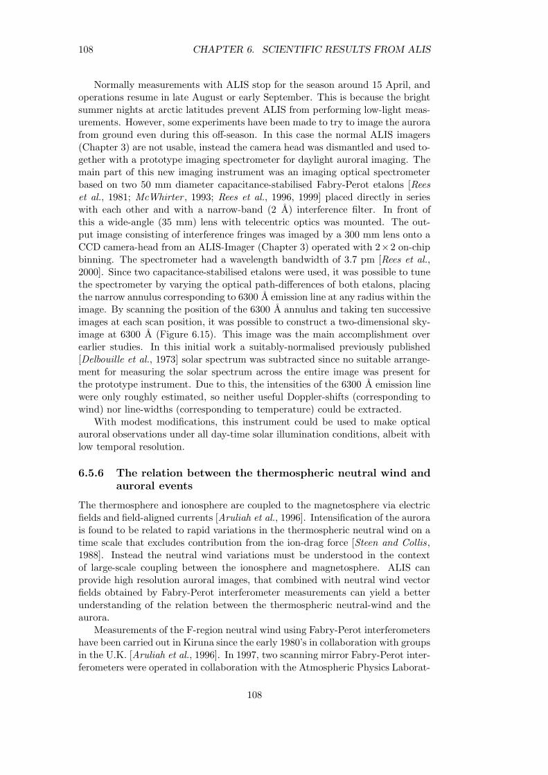
108 CHAPTER 6. SCIENTIFIC RESULTS FROM ALIS
Normally measurements with ALIS stop for the season around 15 April, andoperations resume in late August or early September. This is because the brightsummer nights at arctic latitudes prevent ALIS from performing low-light meas-urements. However, some experiments have been made to try to image the aurorafrom ground even during this off-season. In this case the normal ALIS imagers(Chapter 3) are not usable, instead the camera head was dismantled and used to-gether with a prototype imaging spectrometer for daylight auroral imaging. Themain part of this new imaging instrument was an imaging optical spectrometerbased on two 50 mm diameter capacitance-stabilised Fabry-Perot etalons [Reeset al., 1981; McWhirter , 1993; Rees et al., 1996, 1999] placed directly in serieswith each other and with a narrow-band (2 A) interference filter. In front ofthis a wide-angle (35 mm) lens with telecentric optics was mounted. The out-put image consisting of interference fringes was imaged by a 300 mm lens onto aCCD camera-head from an ALIS-Imager (Chapter 3) operated with 2×2 on-chipbinning. The spectrometer had a wavelength bandwidth of 3.7 pm [Rees et al.,2000]. Since two capacitance-stabilised etalons were used, it was possible to tunethe spectrometer by varying the optical path-differences of both etalons, placingthe narrow annulus corresponding to 6300 A emission line at any radius within theimage. By scanning the position of the 6300 A annulus and taking ten successiveimages at each scan position, it was possible to construct a two-dimensional sky-image at 6300 A (Figure 6.15). This image was the main accomplishment overearlier studies. In this initial work a suitably-normalised previously published[Delbouille et al., 1973] solar spectrum was subtracted since no suitable arrange-ment for measuring the solar spectrum across the entire image was present forthe prototype instrument. Due to this, the intensities of the 6300 A emission linewere only roughly estimated, so neither useful Doppler-shifts (corresponding towind) nor line-widths (corresponding to temperature) could be extracted.
With modest modifications, this instrument could be used to make opticalauroral observations under all day-time solar illumination conditions, albeit withlow temporal resolution.
6.5.6 The relation between the thermospheric neutral wind andauroral events
The thermosphere and ionosphere are coupled to the magnetosphere via electricfields and field-aligned currents [Aruliah et al., 1996]. Intensification of the aurorais found to be related to rapid variations in the thermospheric neutral wind on atime scale that excludes contribution from the ion-drag force [Steen and Collis,1988]. Instead the neutral wind variations must be understood in the contextof large-scale coupling between the ionosphere and magnetosphere. ALIS canprovide high resolution auroral images, that combined with neutral wind vectorfields obtained by Fabry-Perot interferometer measurements can yield a betterunderstanding of the relation between the thermospheric neutral-wind and theaurora.
Measurements of the F-region neutral wind using Fabry-Perot interferometershave been carried out in Kiruna since the early 1980’s in collaboration with groupsin the U.K. [Aruliah et al., 1996]. In 1997, two scanning mirror Fabry-Perot inter-ferometers were operated in collaboration with the Atmospheric Physics Laborat-
108
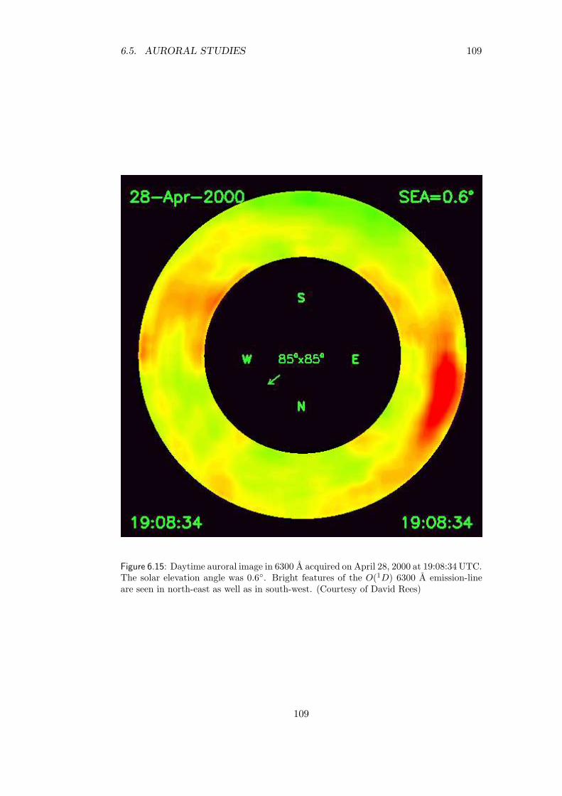
6.5. AURORAL STUDIES 109
Figure 6.15: Daytime auroral image in 6300 A acquired on April 28, 2000 at 19:08:34 UTC.The solar elevation angle was 0.6. Bright features of the O(1D) 6300 A emission-lineare seen in north-east as well as in south-west. (Courtesy of David Rees)
109
110 CHAPTER 6. SCIENTIFIC RESULTS FROM ALIS
ory at University College London [McWhirter , 1993; Aruliah et al., 1996], as wellas one Doppler Imaging System (DIS) [Rees et al., 1997] in collaboration withUtah State University and Hovemere Ltd. In a preliminary study [Brandstromet al., 1997b] data from the latter instrument was compared to auroral imagesobtained from ALIS. The Doppler Imaging System (DIS) used in Kiruna consistsof an all-sky lens, an interference filter for the 6300A airglow/auroral emissionand a Fabry-Perot etalon. The resulting interference fringes are imaged by anintensified Peltier-cooled CCD camera. In the subsequent analysis, each of the sixinterference fringes are divided into 24 sectors for which the Doppler shift of theinput signal is calculated. Each sector thus corresponds to the Doppler-shift in acertain region of the sky, making it possible to ‘image’ the neutral wind velocity.
During the winter of 1996/1997 events with conjugate all-sky, ALIS and DISobservations were collected. Events when there was clear sky, auroral activity andpreferably discrete auroral forms with a strong signal in the O(1D) 6300 A emis-sion line were selected. A collection of data from 10 January 1997 was describedby Brandstrom et al. [1997b]. (Other promising events also exist for example7–9 February 1997). When a stable arc was seen, the neutral wind was mainlynorthward. Preliminary analysis of the dataset suggests that the wind is directedperpendicular to the arc, with very low wind speeds parallel to the arc. Thisobservation is supported by observations from 10 January. Another interestingfeature in the data is the apparent westward drift of diffuse auroral structuresat the same time as the wind turns eastward around 19:30 UTC. However theseresults are to be considered only as a demonstration of measurement possibilities.These studies have not been followed up so far.
6.6 Other studies
6.6.1 Polar stratospheric clouds
ALIS was optimised for studies of auroral phenomena at altitudes ranging from90–300 km (Chapter 2). Despite this, it was realised early [Steen, 1989; Steenet al., 1990] that ALIS might also be useful for the study of PSCs. Such cloudsoccur when regions of liquid or solid aerosols form in the altitude range of 15–30 km due to the low stratospheric temperatures that can be reached during thepolar night in Arctic and Antarctic polar vortex combined with the additionalrapid cooling caused by lee-waves [for example Hesstvedt , 1960; Toon et al., 1986;Crutzen and Arnold , 1986; Tolbert , 1996, and references therein]. PSCs have beenobserved for more than a hundred years and Mohn [1893] attempted to make analtitude estimation by visual observations but arrived at uncertain results (23–100 km). One of the first accurate measurements of PSC altitude was performedby Størmer [1930], using photographic triangulation techniques. The presenceof stratospheric clouds causes increased stratospheric ozone depletion [Solomonet al., 1986] and because of this, the interest in PSC studies increased at the endof the last century.
ALIS is used to detect the appearance of PSCs and also to obtain temporalvariation in the 3D distribution of the cloud surfaces. In 1997 ALIS made PSCobservations, presenting a temporal development of the two-dimensional altitude
110
6.6. OTHER STUDIES 111
distribution during three events, 9, 11 and 16 January 1997 [Steen et al., 1997b].Measurement techniques and the derivation of a composite colour image (derivedfrom three images obtained with narrow-band interference filters for the threemain auroral lines 6300 A, 5577 A and 4278 A) are presented in Steen et al.[1999b] and Enell et al. [1999c]. According to Steen et al. [1999b] “it would, atleast in principle be possible to invert the particle size distribution in the PSC bymeasuring the absolute colour variation, 3-D surface location, wind parametersand temperature, using an optical transport model”. Enell et al. [1999b] statesthat, in certain cases, it might be possible to retrieve the particle size distributionin a section across the PSC from narrow-band images in several wavelengths. Anexample of time development of an altitude contour of PSC cloud-bases calculatedby triangulation was also presented in this paper.
A feasibility study regarding the use of multi-station imaging systems forstudies of PSC physics was presented by Enell et al. [2000], proposing a methodto solve for particle sizes using bistatic multi-wavelength observations. As ithas not yet been possible to apply this method to real measurements, numer-ical simulations for an ideal case (single scattering, spherical particles) work withreasonable results, even if random noise is added. Despite these positive results,a major complication is that light is scattered not only from the cloud particles,but also from the entire atmospheric column observed. A background correction,assuming a smoothly varying atmospheric background must therefore be applied.An example of a background correction by quad-tree decomposition is discussedby Enell et al. [1999a]. Should this method prove to be practically applicable, animportant issue might be to determine the probability that actual PSC incidencegives rise to visually observable mother-of-pearl clouds, for example for interpret-ation of historical reports of PSC sightings. Such studies would be of interest formodellers of atmospheric chemistry and radiative transfer.
Enell et al. [2003] presented a case study of the development of visible PSCsobserved by ALIS. The paper concerns automatic and manual altitude determ-ination of PSC observations made on 9 January 1997 from two ALIS stations(Figure 6.16). It is shown that semi-automatic detection of stratospheric clouds ispossible, and that short-term dynamics such as altitude variations can be tracked.The PSCs, observed during twilight, were found to be moving within a stationarysloping surface, and some evidence was provided that they were lee-wave induced.Enell et al. [2003] suggests that in future studies “it would be desirable to im-age PSC with polarisation-sensitive devices in order to characterise the scatteredlight with a full set of Stokes parameters at different wavelengths. This might bea way to yield information about the particle shapes as well as the nature of themultiple scattered light illuminating the PSCs.” Furthermore, imaging of PSCsunder different conditions, i.e. direct or scattered sunlight, moon-light, and evenextinction of starlight, deserves further experimental investigations. The PSCevents summarised here were published by Enell [2002]. This work constitutesthe main reference for PSC observations with ALIS.
111
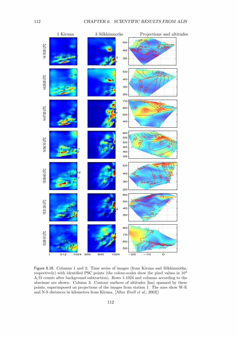
112 CHAPTER 6. SCIENTIFIC RESULTS FROM ALIS
14:19
:30 U
TC
1 2 3 4
5 6 7
8 9101112
13
1 512 1024
1 2
3 4
5
6 7 8 9
10
1112
13
600 800 1024
PSfrag replacements1 Kiruna 3 Silkkimuotka
Projections and altitudes
Altitude surfaces −20 −10 0 10
30
40
50
23.5
23.523.5
23.5
2424
24
2424
24
24
24
24
24.524.5
24.5
PSfrag replacements
1 Kiruna3 Silkkimuotka
Projections and altitudes
Altitude surfaces
14:25
:00 U
TC
12
3 456 7
89
1 512 1024
12
3 45
6 7
89
600 800 1024
PSfrag replacements
−15 −10 −5 0 5
20
30
40
50 22.52323.5
2424
24.5
PSfrag replacements
14:47
:00 U
TC
1 2 3
4 5 6
7 8
910
1112
1 512 1024
1 2 3
4
5 6
7 8
910
11
12
600 800 1024
PSfrag replacements
−20 −10 0
40
50
60
70212223
24
25
26
PSfrag replacements
14:56
:10 U
TC
1 2 3 4
5 6 7 8 91011
1213
14
1 512 1024
1
2 3 4 5 6 7
8 910
11 12
1314
600 800 1024
PSfrag replacements
−30 −20 −10 0
35
40
45
50
55
6023
2323.5
24
24
24.5
24.5
25
25
PSfrag replacements
15:09
:40 U
TC
1 2 3 4 5
6 7 8
910
111213
1 512 1024
1 2 3 4
5
6 7 8
910
1112
13
600 800 1024
PSfrag replacements
−20 −10 020
30
40
50 22
22.5
22.5
23
2323.5
23.5
24
24
24
24.5
24.5
24.5
24.5PSfrag replacements
15:21
:30 U
TC 1 2 3 4 5 6 7
8 9 10
1112
13141516
171819
1 512 1024
1 2 3 4
5 6 7
8 9
101112
1314
15161718
19
600 800 1024
PSfrag replacements
−20 −10 0
30
40
50
60
212223
23
24
24
25
PSfrag replacements
15:29
:10 U
TC
1 2 3 4 5
6 7 8 91011
12
131415
1617
1 512 1024
1 2 3 4 5 6
7 8
910
11
1213
141516 17
600 800 1024
PSfrag replacements
−20 −10 0
50
60
70
80
24
242628
30
PSfrag replacements
Figure 6.16: Columns 1 and 2: Time series of images (from Kiruna and Silkkimuotka,respectively) with identified PSC points (the colour-scales show the pixel values in 104
A/D counts after background subtraction). Rows 1-1024 and columns according to theabscissae are shown. Column 3: Contour surfaces of altitudes [km] spanned by thesepoints, superimposed on projections of the images from station 1. The axes show W-Eand N-S distances in kilometres from Kiruna. [After Enell et al., 2003])
112

6.6. OTHER STUDIES 113
6.6.2 Astronomical applications — water in a Leonid?
Vi missade pa Mars, kom ur dess banaoch for att undga faltet Jupitervi lade oss pa kurvan ICE-tolvi Magdalenafaltets yttre ring,men motte stora mangder leonideroch vajde vidare mot Yko-nio.Vid faltet Sari-sexton uppgav vi forsokenatt vanda om.
Harry Martinsson, Aniara
Early on it was realised that ALIS might be usable for spectroscopic studies ofcertain astronomical objects, such as comets and meteoroids ejected from comets.Images were acquired of both the Hyakutake and Hale-Bopp comets, howevernone of these data-sets have yet been analysed.
Meteor showers are one of few processes taking place above the tropospherethat are observable by the naked eye. This influx of extraterrestrial matter toEarth, on the order of 100 tons per day [Love and Brownlee, 1993] gives rise to thepermanent layer of metal atoms in the 80–110 km altitude region [Hoffner andvon Zahn, 1999]. The study of these phenomena has important implications withrespect to irregularities in long range radio communications, sporadic E-layers,as well as the survivability of artificial satellites, etc.
Modelling studies [McNeil et al., 1995, 2001] combined with LIDAR observa-tions [Hoffner and von Zahn, 1999; von Zahn et al., 1999] as well as observationsby the GLO-1 instrument on the space-shuttle [Gardner et al., 1999] have yiel-ded significant new information on the mechanisms involved in the formation ofmeteor-trails and their properties.
When cosmic dust particles enters the Earth’s atmosphere, heating and ab-lation of the material causes deposition of metals at altitudes between 80 and110 km. As the atmospheric density increases exponentially along the particletrajectory, the ablation increases with decreasing altitude. On the other hand,due to atmospheric friction, the particle eventually reaches its terminal velocity,corresponding to a temperature lower than that needed for ablation to take place.Particle mass and particle velocity determine the altitude at which ablation takesplace. Given high enough velocity (about 30 km/s) a particle ablates completely,otherwise parts of the material fall to ground unablated [McNeil et al., 1998].In essence this means that different elements are released from the meteor atdifferent times, as demonstrated by von Zahn et al. [1999] using ground-basedLIDARs.
ALIS could be used to study such differential ablation phenomena in meteortrails. The easiest meteoroid constituents to observe are the quite common so-dium (Na) and calcium (Ca). These elements have strong emission lines at 5893 Aand 4227 A [Ceplecha and Rajchl , 1963]. The evaporation is a temperature-dependent process for the different constituents. According to the differentialablation model there is a distinct altitude difference of several kilometres for thesodium and calcium deposition distributions. This should be quite easily seenwith two or more ALIS stations equipped with the proper filters, especially forslow meteors. However, there are other practical problems concerning observa-
113

114 CHAPTER 6. SCIENTIFIC RESULTS FROM ALIS
tions of this type. A meteor is most often seen during a short interval of just onesecond or less, and this must occur while the shutter is open. To maximise thepossibility of acquiring an image of a meteor-trail, the stations should be operatedwith overlapping exposures, so that there are always at least two imagers withopen shutters. In this way simultaneous imaging from up to six stations mightoccur, so that the altitude distribution of the meteor trails could be triangulated,while some stations simultaneously image the trails in the rather strong sodium(5893 A) and calcium (4227 A) emission lines [Ceplecha and Rajchl , 1963].
In a simulated study [Brandstrom et al., 2001a] it was suggested that ALISwould operate with all six stations. The imagers would be oriented to observea common volume, in order to enable triangulation of altitudes. The CCD-detectors are operated in maximum resolution mode (1024 × 1024 pixels) andwith the longest possible integration times without saturating the CCD (on theorder of several minutes). The dynamics is recorded by quickly opening andclosing the shutter, with a period of 50 ms. (In principle this should be possible,but there are still some technical problems to be solved. Another option is toinstall a separate “meteor-shutter”.) Performing the observations in this wayincreases the probability of observing a meteor and gives the possibility to studythe velocities of a particular meteor at different altitudes.
In order to attempt experiments involving meteor observations, two filterswith suitable passbands were procured (Table 6.5).
λcw [A] ∆λ [A] corr. passband [A] usage
4227 280 4087–4356 Covering Ca I and Fe I emission-lines[Ceplecha and Rajchl , 1963] as well asa water band around 4230 A [Dressleret al., 1992]
5893 200 5793–5978 Covering Na emission-lines at 5893 A[Ceplecha and Rajchl , 1963]
Table 6.5: Filters for meteor studies. The table gives centre wavelengths, filter bandwidth,corrected passband and emission lines of interest.
Some preliminary studies were carried out during the Leonid showers of 1996(without the meteor filters), 1999, 2000 and 2001. These observations yieldedno usable results mainly due to bad weather conditions, although, importantknowledge about how to perform an observation of this type was gained. Themain objective with these experimental observations was to try to observe apredicted differential ablation process.
Successful observations of a meteor trail using two adjacent ALIS stations(Kiruna, and the mobile station) were obtained on 19 November 2002, at 03:48UTC. The observed Leonid probably originated from the population ejected fromthe comet 55P/Tempel-Tuttle in 1767 according to the dust-trail simulations andobservations by McNaught and Asher [1999]. Consequently this meteoroid wason its 7th period around the sun and still quite young in the sense that it hadnot lost much of its volatile constituents. Four images of this meteor trail appear
114

6.6. OTHER STUDIES 115
Figure 6.17: Portions of ALIS raw-data images of a meteor trail acquired on November19, 2002. From left to right: (1) A 20 s exposure starting at 03:48:00 UTC in 4227 A.(2) 10 s exposure at 03:48:00 UTC in 5893 A (3) Same filter and integration time, butexposed at 03:48:30 UTC and (3) at 03:49:00 UTC. The false colours correspond to thecolours in Figure 6.18
in Figure 6.17.In Figure 6.18 projected altitude profiles for the images in Figure 6.17 appear.Figure 6.19 shows the meteor-trail projected in altitude versus horizontal
distance scale as observed through the two filters and with intensity profilesfor both wavelengths. The relatively high intensity, the length of the trail aswell as the short life time of the 4227 A component were unexplained from thebeginning. The 5893 A component was seen in three consecutive images rangingover 1.5 minutes while the strong 4227 A emission line was seen only withinone 20 seconds exposure. The 4227 A echo became visible already from 160 kmaltitude while the other one appeared at about 130 km altitude.
Similar optical observations of high-altitude Leonids have been reported from1998 Leonids by Spurny et al. [2000] and there is still no good explanation forthem. While their observations were made in white light, the rather wide pass-band of the filter used for the ALIS-observations might provide a hint as to apossible origin of these unusual high and bright Leonids. The 280 A bandwidthof the 4227 A filter corresponds to a corrected passband of about 4077 A to4356 A (Equation 3.45). Dressler et al. [1992] report luminescence measurementsof N+
2 + H2O supra-thermal charge transfer collisions and have measured hy-drogen atom Balmer series and N+
2 emissions at high energies overlapping thepassband of the ALIS observations. This observation can thus restrict the ori-gin of these high-altitude meteors to one possible explanation. The water is stillbound to some minerals in these young meteors. By reaching temperatures ofabove 1500 K which occurs already at about 130 km altitude in the meteor impactprocess, the water is suddenly released in a fast and bright process.
This explanation was found in March 2003. Therefore the value of observingwater from meteoroides, cannot yet be evaluated, especially in the perspective ofthe present observing instrument ALIS. The analysis of this case continues anda manuscript is in preparation [Pellinen-Wannberg et al., 2003].
115

116 CHAPTER 6. SCIENTIFIC RESULTS FROM ALIS
2500
4000
6000
1000020000 40000
60000
−10 0 10 20 30 40 5080
100
120
140
160
180
200
Figure 6.18: Projected altitude-profile of the raw-data in Figure 6.17. The iso-intensitylines corresponds to the 4227 A image. The red, green and blue colours correspond tothe three images in 5893 A. It is possible to see how the Na emission in the meteor traildrifts with time from 03:48:00 UTC until 03:49:00 UTC.
116
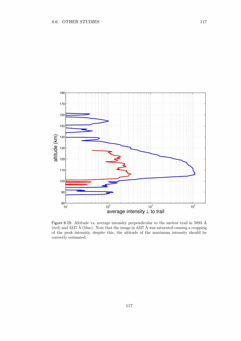
6.6. OTHER STUDIES 117
101 102 103 10480
90
100
110
120
130
140
150
160
170
180
average intensity ⊥ to trail
altit
ude
(km
)
Figure 6.19: Altitude vs. average intensity perpendicular to the meteor trail in 5893 A(red) and 4227 A (blue). Note that the image in 4227 A was saturated causing a croppingof the peak intensity, despite this, the altitude of the maximum intensity should becorrectly estimated.
117

118 CHAPTER 6. SCIENTIFIC RESULTS FROM ALIS
118
119
Chapter 7
Concluding remarks
“Cur invideamus posteritati nostris laboribus frui?Majori laudi ducteur Seculo nostro observationes veras ad posteritatis me-moriam transmisisse, quam falsas & facile refellendas hypotheses.Utinam priora Secula rerum naturalium experientias potius, quam variasopiniones nobis reliquissent!” Celsius [1733]
This report has attempted to provide a thorough documentation of the ALIS-project. Naturally, the focus of this work has been on the design, operationand calibration of the instrument, as this has been the main occupation of thisauthor for more than one decade. Apart from ALIS, which provides imagingspectroscopic absolute-measurements of column emission rates, there has beensome work carried out related to colour imaging of aurora, as is briefly describedin Appendix C.
Since April 2001, only occasional campaigns related to the study of HF pump-enhanced airglow have been carried out with 1–2 stations that were operatedmanually. As there has recently emerged increased interest in a more extensiveoperation of ALIS, an outline of the required actions, as well as some ideas forthe future appear in Appendix D.
Chapter 6 provided a survey of the versatile scientific applications of a multi-station low-light imaging system such as ALIS. Although many results alreadyhave been obtained, scientific questions that have arisen from this work requirefurther analysis of existing data-sets as well as new measurements.
At present, the scientific highlights from ALIS include the first unambigu-ous observations of HF-pump enhanced aurora [Brandstrom et al., 1999] and thefirst tomographic estimate of volume distribution of HF-pump enhanced airglowemissions [Gustavsson et al., 2001a]. The task of following up some of the newscientific questions raised by these observations would alone motivate the con-tinued operation of ALIS for many years. The recent promising observations ofLeonid meteor-trails (Section 6.6.2) might also prove to be a fruitful field of futurestudies with ALIS.
As a spin-off effect, the combined use of the ALIS detector together with animaging spectrometer resulted in the first daytime ground-based optical image ofthe aurora which was acquired on 2 May 1999 [Rees et al., 2000].
It can therefore undoubtably be said that there exist strong multi-disciplinaryscientific arguments for the continued operation of ALIS.
119
120 CHAPTER 7. CONCLUDING REMARKS
A reader interested in further information related to three-dimensional ima-ging of the aurora and airglow, geometrical calibration, etc., is recommended tostudy Gustavsson [2000], as these topics were only briefly touched upon in thepresent work. Further reading related to the processing of multi-station auroralimage data is found in the work by Rydesater [2001].
Simultaneous auroral imaging from space-borne optical instruments would bean effective complement to the ground-based images. Ideally a sounding rocketlaunched through an auroral structure, resulting in simultaneous measurementsfrom both ground and space, would certainly provide new insights into the auroralaltitude distribution and the possibility to further validate and enhance the 3D-reconstruction techniques.
Observations of the rich and interesting night-sky phenomena related to au-roral and ionospheric space plasma physics as well as the environmentally import-ant atmospheric physics is a long-term commitment involving many disciplines aswell as ground-based and space-borne instruments of various types. The diversityof the scientific results summarised in this chapter provides an example of whatcan be achieved on a moderate budget.
In this field of science, long-term stability, not only in terms of continuousobservations, but also in terms of budget and staffing, combined with long-termplans for technical maintenance and development is important.
120
121
Appendix A
The Instrumentation Platform
“It might be the warriors who get the glory, but it’s the engineers who buildsocieties” B’Lanna Torres
Any scientific instrumentation, regardless of whether it is manual or automatic,ground-based or space-borne, needs some basic supporting infrastructure in theform of:
• Structural support of the instrument, for example the satellite platform ora measurement structure with instrument stand.
• Environmental subsystems, keeping environmental parameters (for exampletemperature) within acceptable limits.
• Power supply and conditioning devices.
• Control subsystems. Anything from a simple switch to a sophisticatedtelecommand system.
• Monitoring subsystems. Anything from eyeball observations of an instru-ment reading to a complex telemetry system.
• Communication] subsystems.
• Data processing and storage subsystems.
For space-borne instruments, many of these functions are provided by the space-craft platform. In the ground-based case many of these requirements are oftenmore relaxed due to a less-hostile environment and the proximity to the generalinfrastructure of human civilisation. However if unmanned measurement sta-tions are deployed in a sparsely-populated area with a sub-arctic climate, somerequirements on the instrument platform becomes as demanding as in the space-borne case. Thus the ALIS-project required a closer examination of the basicinfrastructure than most ground-based facilities in the field. The required ba-sic infrastructure for low-light imaging stations could to a large extent also beused by other instruments (not necessarily optical), or even in entirely differentcontexts. Thus, these efforts to provide a housing for the ALIS stations resul-ted in the concept of a Ground-based Low-light Imaging Platform (GLIP) whichconstitutes the major part of an ALIS station.
121
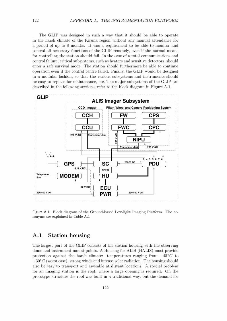
122 APPENDIX A. THE INSTRUMENTATION PLATFORM
The GLIP was designed in such a way that it should be able to operatein the harsh climate of the Kiruna region without any manual attendance fora period of up to 8 months. It was a requirement to be able to monitor andcontrol all necessary functions of the GLIP remotely, even if the normal meansfor controlling the station should fail. In the case of a total communication- andcontrol failure, critical subsystems, such as heaters and sensitive detectors, shouldenter a safe survival mode. The station should furthermore be able to continueoperation even if the control centre failed. Finally, the GLIP would be designedin a modular fashion, so that the various subsystems and instruments shouldbe easy to replace for maintenance, etc. The major subsystems of the GLIP aredescribed in the following sections; refer to the block diagram in Figure A.1.
MODEM
Transputer−link
CCH
CCU230 V AC
CCD−Imager
FWC
FW CPS
CPC
NIPU
230
V A
C
Filter−Wheel and Camera Positioning System
Transputer−link 230 V AC
ALIS Imager Subsystem
Telephoneline
SC
HU
PDU12 4 8 7 653
ECUPWR
GPS
Ant.
GLIP
230/400 V AC
12 V DC
12 V DC
RS232
230/400 V AC
230 V AC
Figure A.1: Block diagram of the Ground-based Low-light Imaging Platform. The ac-ronyms are explained in Table A.1
A.1 Station housing
The largest part of the GLIP consists of the station housing with the observingdome and instrument mount points. A Housing for ALIS (HALIS) must provideprotection against the harsh climate: temperatures ranging from −45C to+30C (worst case), strong winds and intense solar radiation. The housing shouldalso be easy to transport and assemble at distant locations. A special problemfor an imaging station is the roof, where a large opening is required. On theprototype structure the roof was built in a traditional way, but the demand for
122
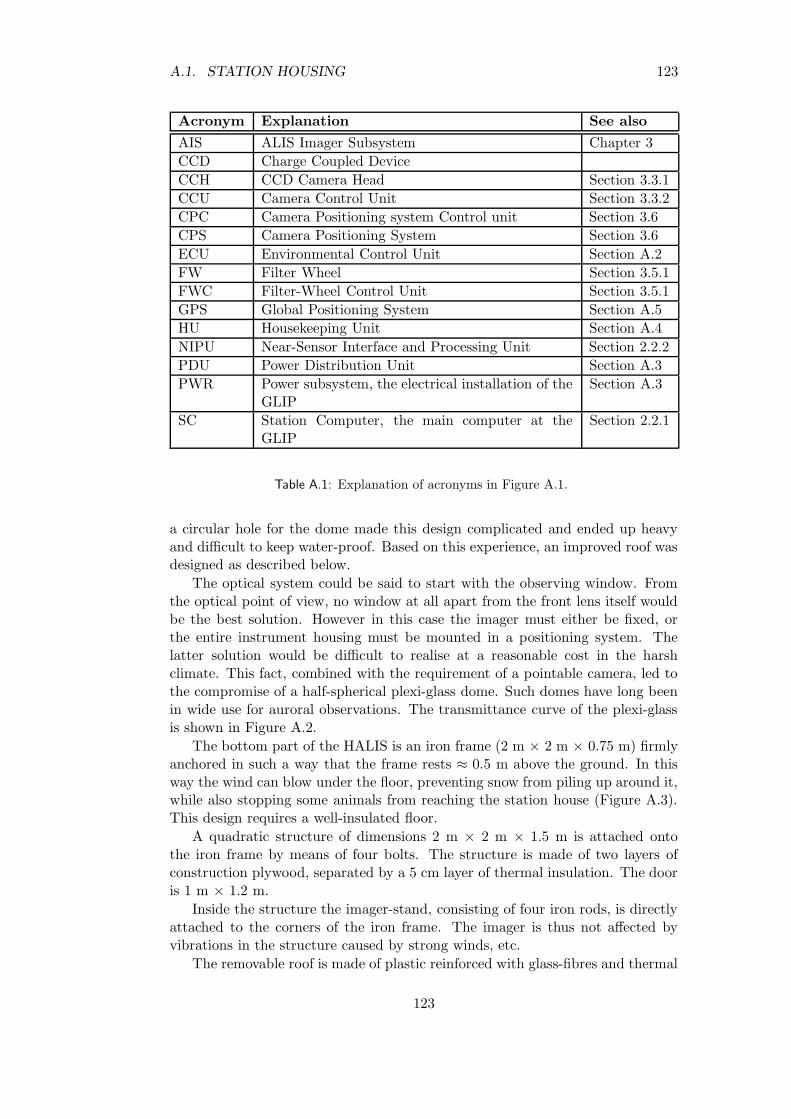
A.1. STATION HOUSING 123
Acronym Explanation See also
AIS ALIS Imager Subsystem Chapter 3
CCD Charge Coupled Device
CCH CCD Camera Head Section 3.3.1
CCU Camera Control Unit Section 3.3.2
CPC Camera Positioning system Control unit Section 3.6
CPS Camera Positioning System Section 3.6
ECU Environmental Control Unit Section A.2
FW Filter Wheel Section 3.5.1
FWC Filter-Wheel Control Unit Section 3.5.1
GPS Global Positioning System Section A.5
HU Housekeeping Unit Section A.4
NIPU Near-Sensor Interface and Processing Unit Section 2.2.2
PDU Power Distribution Unit Section A.3
PWR Power subsystem, the electrical installation of theGLIP
Section A.3
SC Station Computer, the main computer at theGLIP
Section 2.2.1
Table A.1: Explanation of acronyms in Figure A.1.
a circular hole for the dome made this design complicated and ended up heavyand difficult to keep water-proof. Based on this experience, an improved roof wasdesigned as described below.
The optical system could be said to start with the observing window. Fromthe optical point of view, no window at all apart from the front lens itself wouldbe the best solution. However in this case the imager must either be fixed, orthe entire instrument housing must be mounted in a positioning system. Thelatter solution would be difficult to realise at a reasonable cost in the harshclimate. This fact, combined with the requirement of a pointable camera, led tothe compromise of a half-spherical plexi-glass dome. Such domes have long beenin wide use for auroral observations. The transmittance curve of the plexi-glassis shown in Figure A.2.
The bottom part of the HALIS is an iron frame (2 m × 2 m × 0.75 m) firmlyanchored in such a way that the frame rests ≈ 0.5 m above the ground. In thisway the wind can blow under the floor, preventing snow from piling up around it,while also stopping some animals from reaching the station house (Figure A.3).This design requires a well-insulated floor.
A quadratic structure of dimensions 2 m × 2 m × 1.5 m is attached ontothe iron frame by means of four bolts. The structure is made of two layers ofconstruction plywood, separated by a 5 cm layer of thermal insulation. The dooris 1 m × 1.2 m.
Inside the structure the imager-stand, consisting of four iron rods, is directlyattached to the corners of the iron frame. The imager is thus not affected byvibrations in the structure caused by strong winds, etc.
The removable roof is made of plastic reinforced with glass-fibres and thermal
123
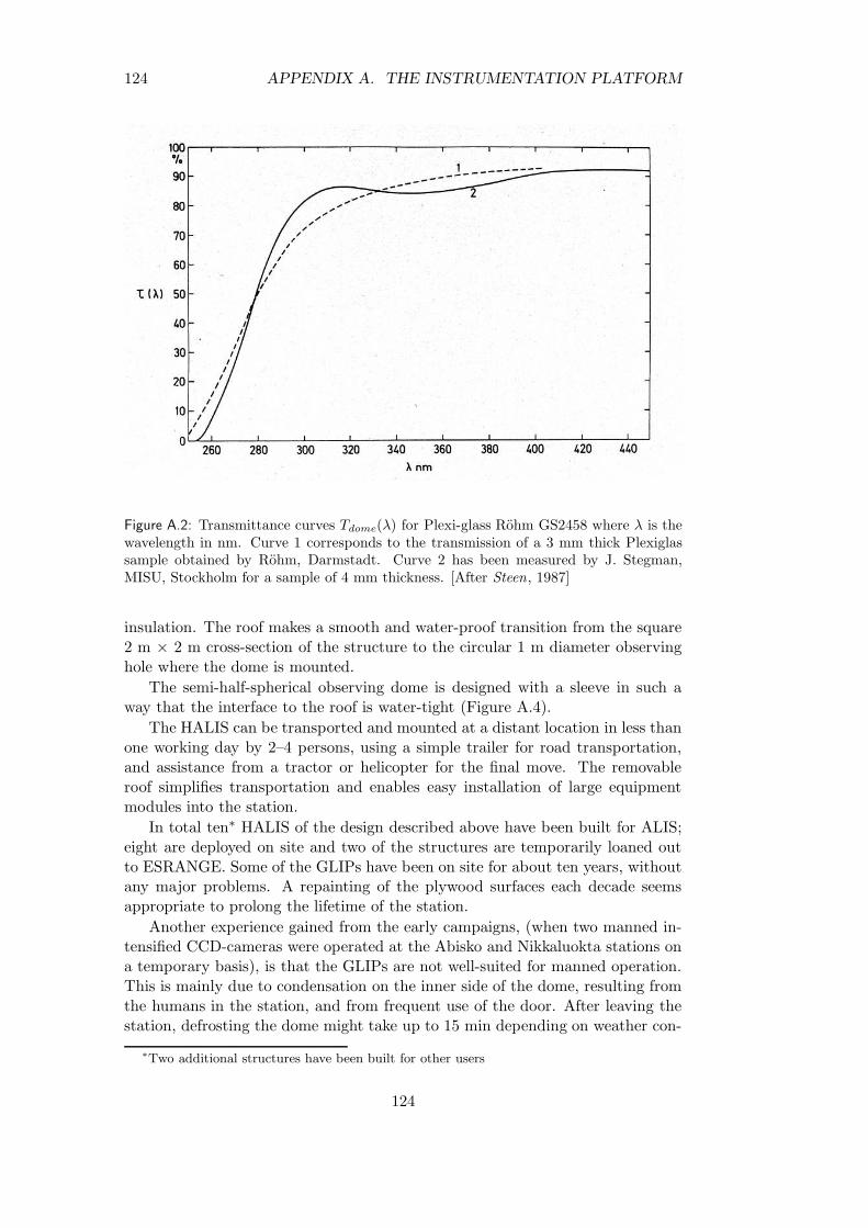
124 APPENDIX A. THE INSTRUMENTATION PLATFORM
Figure A.2: Transmittance curves Tdome(λ) for Plexi-glass Rohm GS2458 where λ is thewavelength in nm. Curve 1 corresponds to the transmission of a 3 mm thick Plexiglassample obtained by Rohm, Darmstadt. Curve 2 has been measured by J. Stegman,MISU, Stockholm for a sample of 4 mm thickness. [After Steen, 1987]
insulation. The roof makes a smooth and water-proof transition from the square2 m × 2 m cross-section of the structure to the circular 1 m diameter observinghole where the dome is mounted.
The semi-half-spherical observing dome is designed with a sleeve in such away that the interface to the roof is water-tight (Figure A.4).
The HALIS can be transported and mounted at a distant location in less thanone working day by 2–4 persons, using a simple trailer for road transportation,and assistance from a tractor or helicopter for the final move. The removableroof simplifies transportation and enables easy installation of large equipmentmodules into the station.
In total ten∗ HALIS of the design described above have been built for ALIS;eight are deployed on site and two of the structures are temporarily loaned outto ESRANGE. Some of the GLIPs have been on site for about ten years, withoutany major problems. A repainting of the plywood surfaces each decade seemsappropriate to prolong the lifetime of the station.
Another experience gained from the early campaigns, (when two manned in-tensified CCD-cameras were operated at the Abisko and Nikkaluokta stations ona temporary basis), is that the GLIPs are not well-suited for manned operation.This is mainly due to condensation on the inner side of the dome, resulting fromthe humans in the station, and from frequent use of the door. After leaving thestation, defrosting the dome might take up to 15 min depending on weather con-
∗Two additional structures have been built for other users
124
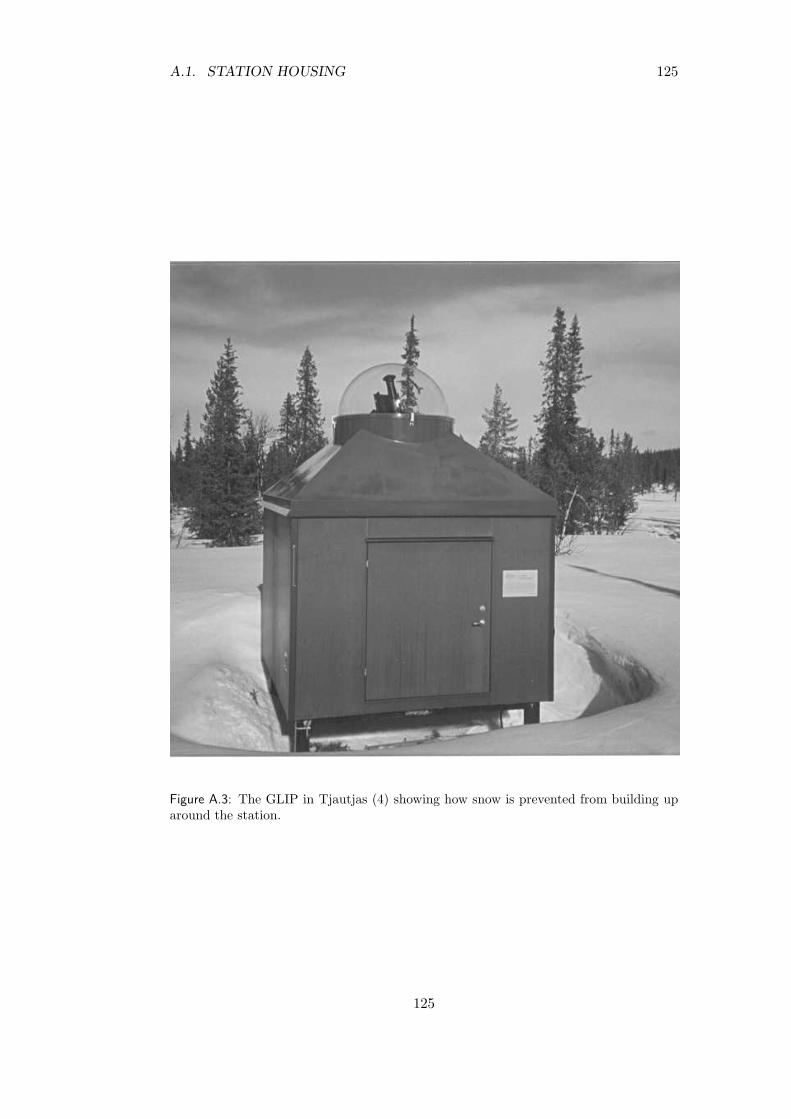
A.1. STATION HOUSING 125
Figure A.3: The GLIP in Tjautjas (4) showing how snow is prevented from building uparound the station.
125
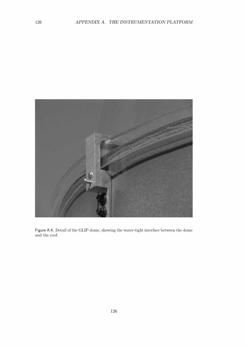
126 APPENDIX A. THE INSTRUMENTATION PLATFORM
Figure A.4: Detail of the GLIP dome, showing the water-tight interface between the domeand the roof.
126
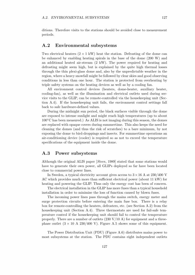
A.2. ENVIRONMENTAL SUBSYSTEMS 127
ditions. Therefore visits to the stations should be avoided close to measurementperiods.
A.2 Environmental subsystems
Two electrical heaters (2 × 1 kW) heat the station. Defrosting of the dome canbe enhanced by enabling heating spirals in the base of the dome (200 W) andan additional heated air-stream (2 kW). The power required for heating anddefrosting might seem high, but is explained by the quite high thermal lossesthrough the thin plexi-glass dome and, also by the unpredictable weather in theregion, where a heavy snowfall might be followed by clear skies and good observingconditions in less than one hour. The station is protected from overheating bytriple safety systems on the heating devices as well as by a cooling fan.
All environment control devices (heaters, dome-heater, auxiliary heater,cooling-fan), as well as the illumination and electrical outlets used during ser-vice visits to the GLIP, can be remote-controlled via the housekeeping unit (Sec-tion A.4). If the housekeeping unit fails, the environment control settings fallback to safe hardware-defined values.
During the midnight sun period, the black surfaces visible through the domeare exposed to intense sunlight and might reach high temperatures (up to about100C has been measured.) As ALIS is not imaging during this season, the domesare replaced with opaque covers during summertime. This also keeps the need forcleaning the domes (and thus the risk of scratches) to a bare minimum, by notexposing the dome to bird-droppings and insects. For summertime operations anair-conditioning device (cooler) is required so as not to exceed the temperaturespecifications of the equipment inside the dome.
A.3 Power subsystems
Although the original ALIS paper [Steen, 1989] stated that some stations wouldhave to generate their own power, all GLIPs deployed so far have been locatedclose to commercial power lines.
In Sweden, a typical electricity account gives access to 3× 16 A at 230/400 VAC which provides much more than sufficient electrical power (about 11 kW) forheating and powering the GLIP. Thus only the energy cost has been of concern.
The electrical installation in the GLIP has more fuses than a typical householdinstallation in order to minimise the loss of function caused by blown fuses.
The incoming power lines pass through the mains switch, energy meter andsurge protection circuits before entering the main fuse box. There is a relaybox for remote-controlling the heaters, defrosters, etc. (see Section A.2) from thehousekeeping unit (Section A.4). Three thermostats are used for fail-safe tem-perature control if the housekeeping unit should fail to control the temperatureproperly. There are a number of outlets (230 V/10 A) for equipment and a three-phase outlet (3 × 10 A 230/400 V). Figure A.5 shows some of this equipment.
The Power Distribution Unit (PDU) (Figure A.6) distributes mains power tomost subsystems at the station. The PDU contains eight independent outlets
127
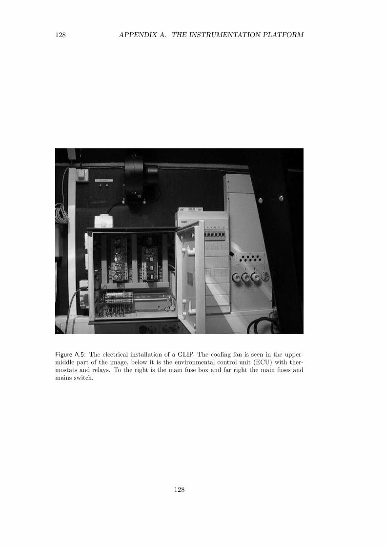
128 APPENDIX A. THE INSTRUMENTATION PLATFORM
Figure A.5: The electrical installation of a GLIP. The cooling fan is seen in the upper-middle part of the image, below it is the environmental control unit (ECU) with ther-mostats and relays. To the right is the main fuse box and far right the main fuses andmains switch.
128
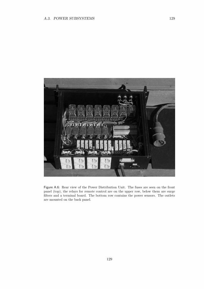
A.3. POWER SUBSYSTEMS 129
Figure A.6: Rear view of the Power Distribution Unit. The fuses are seen on the frontpanel (top), the relays for remote control are on the upper row, below them are surgefilters and a terminal board. The bottom row contains the power sensors. The outletsare mounted on the back panel.
129
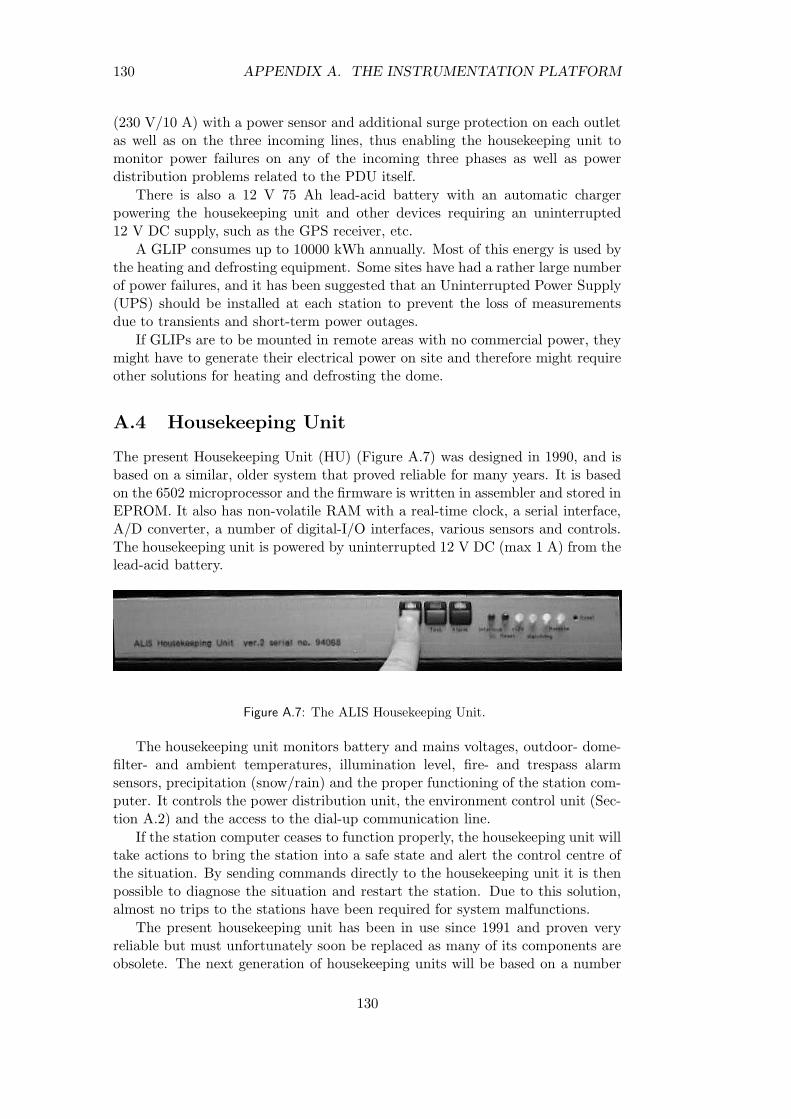
130 APPENDIX A. THE INSTRUMENTATION PLATFORM
(230 V/10 A) with a power sensor and additional surge protection on each outletas well as on the three incoming lines, thus enabling the housekeeping unit tomonitor power failures on any of the incoming three phases as well as powerdistribution problems related to the PDU itself.
There is also a 12 V 75 Ah lead-acid battery with an automatic chargerpowering the housekeeping unit and other devices requiring an uninterrupted12 V DC supply, such as the GPS receiver, etc.
A GLIP consumes up to 10000 kWh annually. Most of this energy is used bythe heating and defrosting equipment. Some sites have had a rather large numberof power failures, and it has been suggested that an Uninterrupted Power Supply(UPS) should be installed at each station to prevent the loss of measurementsdue to transients and short-term power outages.
If GLIPs are to be mounted in remote areas with no commercial power, theymight have to generate their electrical power on site and therefore might requireother solutions for heating and defrosting the dome.
A.4 Housekeeping Unit
The present Housekeeping Unit (HU) (Figure A.7) was designed in 1990, and isbased on a similar, older system that proved reliable for many years. It is basedon the 6502 microprocessor and the firmware is written in assembler and stored inEPROM. It also has non-volatile RAM with a real-time clock, a serial interface,A/D converter, a number of digital-I/O interfaces, various sensors and controls.The housekeeping unit is powered by uninterrupted 12 V DC (max 1 A) from thelead-acid battery.
Figure A.7: The ALIS Housekeeping Unit.
The housekeeping unit monitors battery and mains voltages, outdoor- dome-filter- and ambient temperatures, illumination level, fire- and trespass alarmsensors, precipitation (snow/rain) and the proper functioning of the station com-puter. It controls the power distribution unit, the environment control unit (Sec-tion A.2) and the access to the dial-up communication line.
If the station computer ceases to function properly, the housekeeping unit willtake actions to bring the station into a safe state and alert the control centre ofthe situation. By sending commands directly to the housekeeping unit it is thenpossible to diagnose the situation and restart the station. Due to this solution,almost no trips to the stations have been required for system malfunctions.
The present housekeeping unit has been in use since 1991 and proven veryreliable but must unfortunately soon be replaced as many of its components areobsolete. The next generation of housekeeping units will be based on a number
130
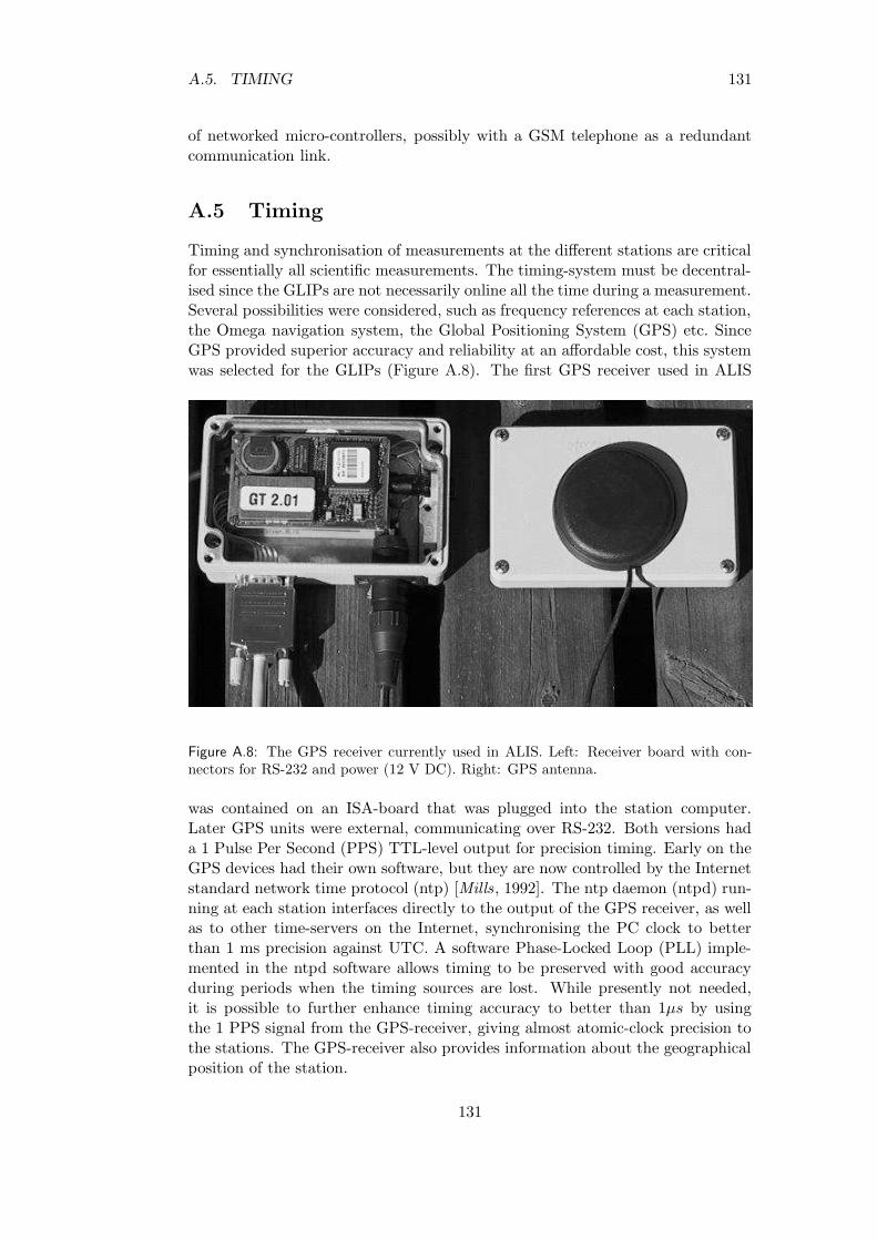
A.5. TIMING 131
of networked micro-controllers, possibly with a GSM telephone as a redundantcommunication link.
A.5 Timing
Timing and synchronisation of measurements at the different stations are criticalfor essentially all scientific measurements. The timing-system must be decentral-ised since the GLIPs are not necessarily online all the time during a measurement.Several possibilities were considered, such as frequency references at each station,the Omega navigation system, the Global Positioning System (GPS) etc. SinceGPS provided superior accuracy and reliability at an affordable cost, this systemwas selected for the GLIPs (Figure A.8). The first GPS receiver used in ALIS
Figure A.8: The GPS receiver currently used in ALIS. Left: Receiver board with con-nectors for RS-232 and power (12 V DC). Right: GPS antenna.
was contained on an ISA-board that was plugged into the station computer.Later GPS units were external, communicating over RS-232. Both versions hada 1 Pulse Per Second (PPS) TTL-level output for precision timing. Early on theGPS devices had their own software, but they are now controlled by the Internetstandard network time protocol (ntp) [Mills, 1992]. The ntp daemon (ntpd) run-ning at each station interfaces directly to the output of the GPS receiver, as wellas to other time-servers on the Internet, synchronising the PC clock to betterthan 1 ms precision against UTC. A software Phase-Locked Loop (PLL) imple-mented in the ntpd software allows timing to be preserved with good accuracyduring periods when the timing sources are lost. While presently not needed,it is possible to further enhance timing accuracy to better than 1µs by usingthe 1 PPS signal from the GPS-receiver, giving almost atomic-clock precision tothe stations. The GPS-receiver also provides information about the geographicalposition of the station.
131
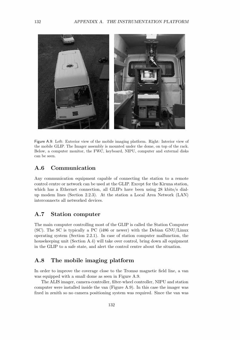
132 APPENDIX A. THE INSTRUMENTATION PLATFORM
Figure A.9: Left: Exterior view of the mobile imaging platform. Right: Interior view ofthe mobile GLIP. The Imager assembly is mounted under the dome, on top of the rack.Below, a computer monitor, the FWC, keyboard, NIPU, computer and external diskscan be seen.
A.6 Communication
Any communication equipment capable of connecting the station to a remotecontrol centre or network can be used at the GLIP. Except for the Kiruna station,which has a Ethernet connection, all GLIPs have been using 28 kbits/s dial-up modem lines (Section 2.2.3). At the station a Local Area Network (LAN)interconnects all networked devices.
A.7 Station computer
The main computer controlling most of the GLIP is called the Station Computer(SC). The SC is typically a PC (i486 or newer) with the Debian GNU/Linuxoperating system (Section 2.2.1). In case of station computer malfunction, thehousekeeping unit (Section A.4) will take over control, bring down all equipmentin the GLIP to a safe state, and alert the control centre about the situation.
A.8 The mobile imaging platform
In order to improve the coverage close to the Tromsø magnetic field line, a vanwas equipped with a small dome as seen in Figure A.9.
The ALIS imager, camera-controller, filter-wheel controller, NIPU and stationcomputer were installed inside the van (Figure A.9). In this case the imager wasfixed in zenith so no camera positioning system was required. Since the van was
132

A.8. THE MOBILE IMAGING PLATFORM 133
manned during the observations, no housekeeping unit, power distribution unit,communications, etc. were required. However if an unmanned, remote-controlledconfiguration had been desired, this equipment could easily have been installed.A mobile generator was also included, so the station was independent of mainspower. This station operated with good results in the years 1999–2003.
133

134 APPENDIX A. THE INSTRUMENTATION PLATFORM
134
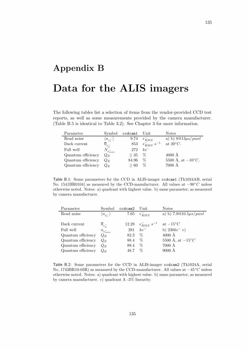
135
Appendix B
Data for the ALIS imagers
The following tables list a selection of items from the vendor-provided CCD testreports, as well as some measurements provided by the camera manufacturer.(Table B.5 is identical to Table 3.2). See Chapter 3 for more information.
Parameter Symbol ccdcam1 Unit Notes
Read noise 〈ne−
r〉 9.74 e−RMS a) b) 8@13µs/pixel
Dark current ne−
d853 e−RMS s−1 at 20C.
Full well Ne−
max272 ke−
Quantum efficiency QE ≥ 35 % 4000 AQuantum efficiency QE 84.96 % 5500 A, at −10C.Quantum efficiency QE ≥ 60 % 7000 A
Table B.1: Some parameters for the CCD in ALIS-imager ccdcam1 (Tk1024AB, serialNo. 1541BR0104) as measured by the CCD-manufacturer. All values at −90C unlessotherwise noted. Notes: a) quadrant with highest value. b) same parameter, as measuredby camera manufacturer.
Parameter Symbol ccdcam2 Unit Notes
Read noise 〈ne−
r〉 7.65 e−RMS a) b) [email protected]µs/pixel
Dark current ne−
d12.28 e−RMS s−1 at −15C
Full well ne−
max281 ke− b) 230ke− c)
Quantum efficiency QE 82.3 % 4000 AQuantum efficiency QE 88.4 % 5500 A, at −15CQuantum efficiency QE 89.4 % 7000 AQuantum efficiency QE 48.7 % 9000 A
Table B.2: Some parameters for the CCD in ALIS-imager ccdcam2 (Tk1024A, serialNo. 1743BR10-03R) as measured by the CCD-manufacturer. All values at −45C unlessotherwise noted. Notes: a) quadrant with highest value. b) same parameter, as measuredby camera manufacturer. c) quadrant A -3% linearity.
135
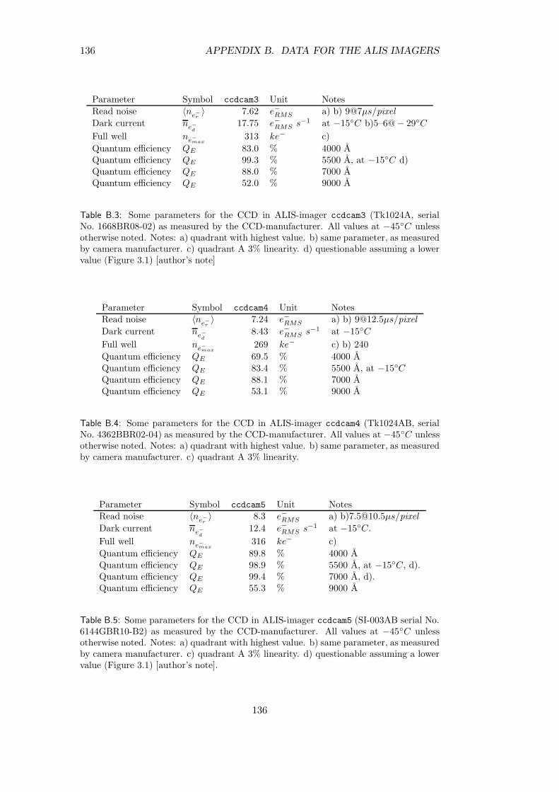
136 APPENDIX B. DATA FOR THE ALIS IMAGERS
Parameter Symbol ccdcam3 Unit Notes
Read noise 〈ne−
r〉 7.62 e−RMS a) b) 9@7µs/pixel
Dark current ne−
d17.75 e−RMS s−1 at −15C b)5–6@− 29C
Full well ne−
max313 ke− c)
Quantum efficiency QE 83.0 % 4000 AQuantum efficiency QE 99.3 % 5500 A, at −15C d)Quantum efficiency QE 88.0 % 7000 AQuantum efficiency QE 52.0 % 9000 A
Table B.3: Some parameters for the CCD in ALIS-imager ccdcam3 (Tk1024A, serialNo. 1668BR08-02) as measured by the CCD-manufacturer. All values at −45C unlessotherwise noted. Notes: a) quadrant with highest value. b) same parameter, as measuredby camera manufacturer. c) quadrant A 3% linearity. d) questionable assuming a lowervalue (Figure 3.1) [author’s note]
Parameter Symbol ccdcam4 Unit Notes
Read noise 〈ne−
r〉 7.24 e−RMS a) b) [email protected]µs/pixel
Dark current ne−
d8.43 e−RMS s−1 at −15C
Full well ne−
max269 ke− c) b) 240
Quantum efficiency QE 69.5 % 4000 AQuantum efficiency QE 83.4 % 5500 A, at −15CQuantum efficiency QE 88.1 % 7000 AQuantum efficiency QE 53.1 % 9000 A
Table B.4: Some parameters for the CCD in ALIS-imager ccdcam4 (Tk1024AB, serialNo. 4362BBR02-04) as measured by the CCD-manufacturer. All values at −45C unlessotherwise noted. Notes: a) quadrant with highest value. b) same parameter, as measuredby camera manufacturer. c) quadrant A 3% linearity.
Parameter Symbol ccdcam5 Unit Notes
Read noise 〈ne−
r〉 8.3 e−RMS a) b)[email protected]µs/pixel
Dark current ne−
d12.4 e−RMS s−1 at −15C.
Full well ne−
max316 ke− c)
Quantum efficiency QE 89.8 % 4000 AQuantum efficiency QE 98.9 % 5500 A, at −15C, d).Quantum efficiency QE 99.4 % 7000 A, d).Quantum efficiency QE 55.3 % 9000 A
Table B.5: Some parameters for the CCD in ALIS-imager ccdcam5 (SI-003AB serial No.6144GBR10-B2) as measured by the CCD-manufacturer. All values at −45C unlessotherwise noted. Notes: a) quadrant with highest value. b) same parameter, as measuredby camera manufacturer. c) quadrant A 3% linearity. d) questionable assuming a lowervalue (Figure 3.1) [author’s note].
136
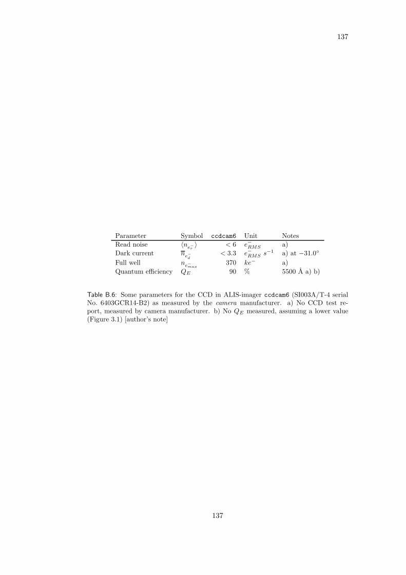
137
Parameter Symbol ccdcam6 Unit Notes
Read noise 〈ne−
r〉 < 6 e−RMS a)
Dark current ne−
d< 3.3 e−RMS s−1 a) at −31.0
Full well ne−
max370 ke− a)
Quantum efficiency QE 90 % 5500 A a) b)
Table B.6: Some parameters for the CCD in ALIS-imager ccdcam6 (SI003A/T-4 serialNo. 6403GCR14-B2) as measured by the camera manufacturer. a) No CCD test re-port, measured by camera manufacturer. b) No QE measured, assuming a lower value(Figure 3.1) [author’s note]
137

138 APPENDIX B. DATA FOR THE ALIS IMAGERS
138
139
Appendix C
Related work
“Hier stehe ich und kann nicht anders.” Martin Luther
When ALIS began operating, an “aiming-system” appeared as desirable. Thiswas planned to consist of a simpler white-light video-rate camera intended mainlyto assist the ALIS operator. Two old low-light TV-cameras were used for thispurpose at the ALIS operations centre. However it was always desired to havereal-time digital colour images available, even if ALIS was operated from a remoteplace. For many years this appeared as impossible or too expensive. Around 1999commercially-available digital still- and video colour cameras began to reach therequired sensitivity. This initiated a study, mainly intended to replace the presentall-sky imager in Kiruna, but also with interesting implications for ALIS. Thisappendix briefly describes these efforts.
It is, however, of great importance to note that the imagers discussed hereare in no way comparable to the ALIS imagers. A colour CCD camera cannever be used for absolute measurements of column emission rates as it containsits own colour filters. On the other hand, the colour cameras can be of greatvalue for providing overview information of the morphology and dynamics. Also,colour images and movies of auroral phenomena tend to be much more appealingfor public outreach purposes, compared to the more scientifically useful, but“unexciting” monochromatic images.
C.1 A new digital all-sky camera
An all-sky camera has been operating in Kiruna since the International Geophys-ical Year in 1957 [Stoffregen, 1962]. In 1977 the camera was replaced with a newmore automated camera [Hypponen et al., 1974]. This camera is still in operation,but a replacement was strongly desired as the data storage medium is 16 mm col-our film, a medium soon to become obsolete, as well as expensive to develop andcopy and difficult to digitise, and thus complicated to make available and distrib-ute to the scientific community and general public. In Finland all 16 mm all-skycameras have already been replaced by advanced new cameras with filter-wheelsand narrow-band interference filters similar to ALIS, but with all-sky optics andintensified CCDs [Syrjasuo, 2001]. Furthermore, a non-intensified spectroscopicall-sky imager is described by Ejiri et al. [1999] (see also Section 1.1). Here an
139
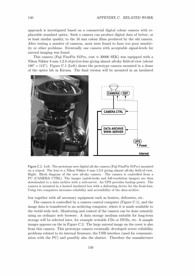
140 APPENDIX C. RELATED WORK
approach is investigated based on a commercial digital colour camera with re-placeable standard optics. Such a camera can produce digital data of better, orat least similar quality, to the 16 mm colour films produced by the old camera.After testing a number of cameras, most were found to have too poor sensitiv-ity or other problems. Eventually one camera with acceptable signal-levels forauroral imaging was found.
This camera (Fuji FinePix S1Pro, cost ≈ 30000 SEK) was equipped with aNikon Nikkor 8 mm 1:2.8 objective-lens giving almost all-sky field-of-view (about180 × 112). Figure C.1 (Left) shows the prototype camera mounted in a domeof the optics lab in Kiruna. The final version will be mounted in an insulated
DEF
DATA ARCHIVEWWW−SERVER
UPS
CAMERA
Internet
Power
CAMERA CTRL
Figure C.1: Left: The prototype new digital all-sky camera (Fuji FinePix S1Pro) mountedon a tripod. The lens is a Nikon Nikkor 8 mm 1:2.8 giving almost all-sky field-of-view.Right: Block diagram of the new all-sky camera. The camera is controlled from aPC (CAMERA CTRL). The images (quick-looks and full-resolution images) are thendownloaded to a data archive with a web-server. An UPS provides backup power. Thecamera is mounted in a heated insulated box with a defrosting device for the front-lens.Using two computers increases reliability and accessibility of the data-archive.
box together with all necessary equipment such as heaters, defrosters, etc.The camera is controlled by a camera control computer (Figure C.1), and the
image data is transferred to an archiving computer, where it is made available tothe world-wide web. Monitoring and control of the camera can be done remotelyusing an ordinary web browser. A data storage medium suitable for long-termstorage will be selected later, for example writable CDs or DVDs, etc. A sampleimages appears on the in Figure C.2. The large auroral image on the cover is alsofrom this camera. This prototype camera eventually developed severe reliabilityproblems related to its internal firmware, the USB interface (used for communic-ation with the PC) and possibly also the shutter. Therefore the manufacturer
140
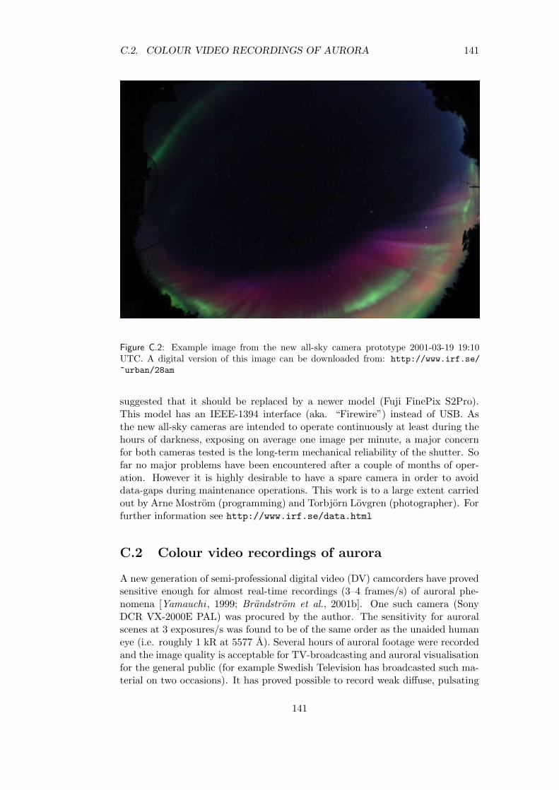
C.2. COLOUR VIDEO RECORDINGS OF AURORA 141
Figure C.2: Example image from the new all-sky camera prototype 2001-03-19 19:10UTC. A digital version of this image can be downloaded from: http://www.irf.se/
~urban/28am
suggested that it should be replaced by a newer model (Fuji FinePix S2Pro).This model has an IEEE-1394 interface (aka. “Firewire”) instead of USB. Asthe new all-sky cameras are intended to operate continuously at least during thehours of darkness, exposing on average one image per minute, a major concernfor both cameras tested is the long-term mechanical reliability of the shutter. Sofar no major problems have been encountered after a couple of months of oper-ation. However it is highly desirable to have a spare camera in order to avoiddata-gaps during maintenance operations. This work is to a large extent carriedout by Arne Mostrom (programming) and Torbjorn Lovgren (photographer). Forfurther information see http://www.irf.se/data.html
C.2 Colour video recordings of aurora
A new generation of semi-professional digital video (DV) camcorders have provedsensitive enough for almost real-time recordings (3–4 frames/s) of auroral phe-nomena [Yamauchi , 1999; Brandstrom et al., 2001b]. One such camera (SonyDCR VX-2000E PAL) was procured by the author. The sensitivity for auroralscenes at 3 exposures/s was found to be of the same order as the unaided humaneye (i.e. roughly 1 kR at 5577 A). Several hours of auroral footage were recordedand the image quality is acceptable for TV-broadcasting and auroral visualisationfor the general public (for example Swedish Television has broadcasted such ma-terial on two occasions). It has proved possible to record weak diffuse, pulsating
141
142 APPENDIX C. RELATED WORK
and black aurora with an acceptable signal-to-noise ratio. These cameras couldtherefore be a good tool for studies of auroral morphology and dynamics, as wellas for providing supporting images for other instruments (ALIS, EISCAT, etc.).Another interesting future possibility is to use this type of camera together withmethods for automated image analysis as described by [for example Rydesater ,2001; Syrjasuo, 2001] for automated control over spectroscopic imaging systemslike ALIS. The following table summarises some of the features of the camcordertested:
• 3 CCD ≈ 450 kpixels.
• Optics: f = 6 − 72 mm 1:1.6-2.4
• 12× optical zoom, 48× digital zoom.
• miniDV tapes (memorystick for still-images)
• IEEE-1394 “Firewire” capture directly to a computer.
• Colour auroral imaging possible from about 3 images per second up to videorate, depending on auroral intensity. Good sensitivity for Red and Greenauroras, acceptable for blue.
A sample frame of an auroral scene with a meteor trail is displayed in Figure C.3.Video footage can be made available by the author on request.
142

C.2. COLOUR VIDEO RECORDINGS OF AURORA 143
Figure C.3: Sample frame from a auroral video obtained with a commercial mini-DVcamcorder displaying green, red and blue aurora. A meteor-trail is seen in the lowermiddle part of the image. A digital version of this image can be downloaded from:http://www.irf.se/~urban/28am
143

144 APPENDIX C. RELATED WORK
144
145
Appendix D
Continued operations withALIS
“Determinismens huvudskal ar kausalitetslagen.Indeterminismens huvudskal ar ansvarskanslan.” Dag Hammarskjold
The design work on ALIS started in 1990. Thus most of the technology of the sys-tem is about ten years old and consequently the need for upgrades and technicalmaintenance has increased. Unfortunately, this has not been possible, mainly be-cause of budgetary constraints. As the measurement season of 2000/2001 ended,ALIS was put into hibernation, mainly to give the author a chance to finish thisreport, but also due to a shortage of staff and funding. Since then, 1–2 ALISimagers have occasionally been operated manually, primarily for studies of HFpump-enhanced airglow. In the fall of 2001 funding covering operation and sometechnical maintenance was received for the period 2002–2004.
From a scientific point of view, a continued and enhanced operation of ALIScan be motivated solely on the new questions raised by the observations of HFpump-enhanced airglow (Section 6.4). The recent promising observations ofmeteor trails (Section 6.6.2), as well as continued auroral studies (Section 6.5)also constitute strong arguments for a prolonged operation of ALIS.
This short appendix outlines how to assess the present status of ALIS in orderto make a plan for bringing ALIS back into full operation. It is assumed thatthe present funding situation is stable for 2003/2004, and that performing newmeasurements, as well as analysing existing data, will enable a sustained fundingat the present level, or higher. The most limited resource for ALIS has alwaysbeen the staff. Here it is assumed that a stable group of at least 3–4 physicists,with a thorough scientific and technical knowledge of ALIS, is available to atleast 50% for engineering and programming tasks, as well as general maintenance.(Ideally ALIS should have access to an electronics engineer and one programmer.However given the present situation this is not considered economically feasible.)
D.1 Assessing the present status of ALIS
Finding out the present status of ALIS is the inevitable first step in making aplan. As ALIS was closed, the status of the system was reported in [Brandstrom,
145
146 APPENDIX D. CONTINUED OPERATIONS WITH ALIS
2001a,b]. Based on this information, an estimate of the efforts required to restartALIS will be presented. It is important to note that in order to make a finalplan, a thorough technical examination of vital systems is required. Such aninvestigation is estimated to take about two man-months (preferably two peoplefor one month). However despite this, it should be possible to start immediatemeasurements with two imagers in parallel as the rest of ALIS is evaluated, theonly constraint being staff availability.
The following list summarises anticipated status of the main technical systems(see also Figure A.1 in Appendix A).
The ALIS stations: In order to save money all stations have been left withelectrical power switched off. To avoid equipment damage, heating shouldbe turned on at least two weeks before attempting to turn on any equipment.The GLIPs (Appendix A) are expected to be found in good condition.However the domes will require cleaning, and some stations might requirerepainting.
Computers: With few exceptions, all computers should be usable. However,all computers are old, and failures cannot be excluded. As each stationcomputer needs at least two ISA-slots for interface boards (NIPU, CCU),it is important to keep the old computers usable as long as possible as newcomputers with ISA slots are becoming rare. Although the NIPU mustbe replaced soon, it is not feasible to replace the CCU within a couple ofyears at the present funding level. Computer replacements must likely bescheduled within 1–2 years.
The NIPU: All NIPUs (Section 2.2.2) were working in 2001, and are expectedto be used at least initially. It must be stressed, however, that the NIPUs aretotally obsolete, they cannot be repaired, nor can any changes to the CPSand FPS be accommodated (for example replacements of angular encoders).As the NIPUs are essential for filter changes, it is important to replace theseunits as soon as possible. They can be replaced by micro-controllers at areasonable cost.
Communication systems: All dial-up telephone lines must be checked. Somemodems might require replacement. It should furthermore be investigatedif station 5 in Abisko can be connected to Internet via the LAN at theAbisko Research Station. Continued efforts should be made to find cheaperand faster communication to the stations. (see also Section 2.2.3)
Station data storage: Most external disks used for local data storage (Sec-tion 2.2.4) at the stations are well past their safe technical lifetime, due tomany hours of operation. They are also small by present standards. Asdisk-crashes at the stations may lead to large data losses, all disks shouldbe replaced. The cost for procuring 10–12 external disks is relatively low.
Data archiving: Documentation and backup copying at alternate sites of theALIS data-base is underway as this is written. It is recommended thatthe archive media be transferred from CD-R (Recordable CD-ROMs) to
146
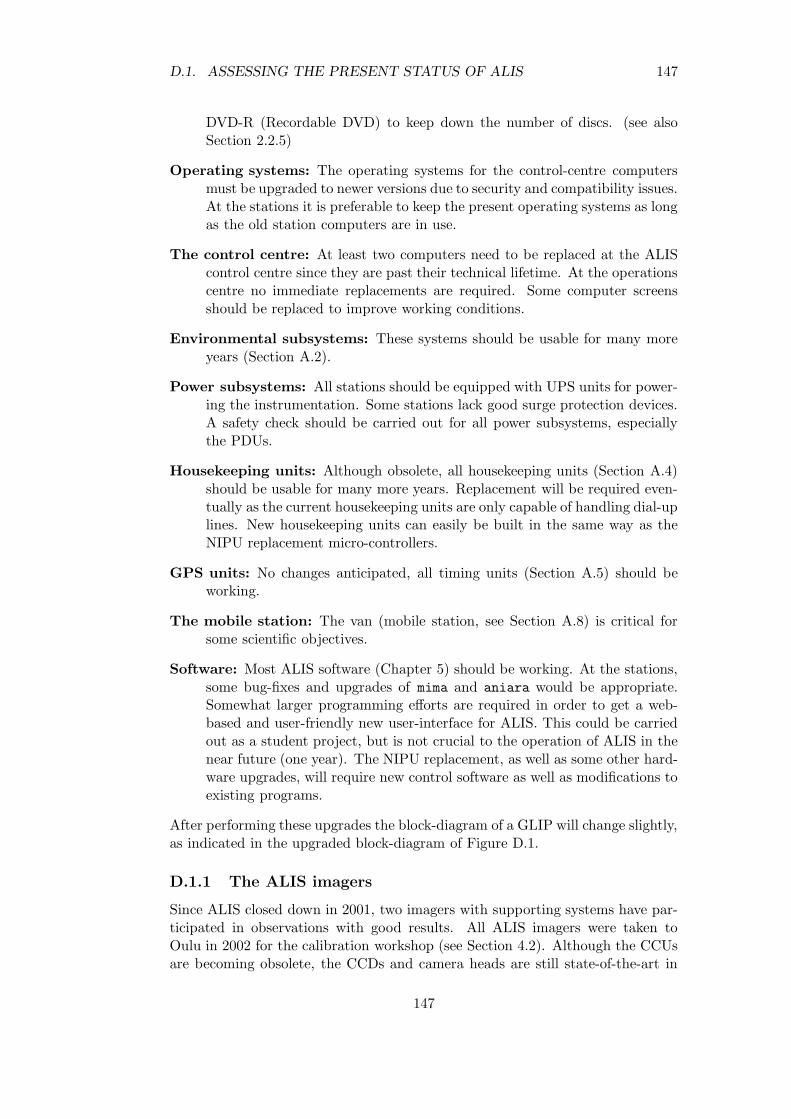
D.1. ASSESSING THE PRESENT STATUS OF ALIS 147
DVD-R (Recordable DVD) to keep down the number of discs. (see alsoSection 2.2.5)
Operating systems: The operating systems for the control-centre computersmust be upgraded to newer versions due to security and compatibility issues.At the stations it is preferable to keep the present operating systems as longas the old station computers are in use.
The control centre: At least two computers need to be replaced at the ALIScontrol centre since they are past their technical lifetime. At the operationscentre no immediate replacements are required. Some computer screensshould be replaced to improve working conditions.
Environmental subsystems: These systems should be usable for many moreyears (Section A.2).
Power subsystems: All stations should be equipped with UPS units for power-ing the instrumentation. Some stations lack good surge protection devices.A safety check should be carried out for all power subsystems, especiallythe PDUs.
Housekeeping units: Although obsolete, all housekeeping units (Section A.4)should be usable for many more years. Replacement will be required even-tually as the current housekeeping units are only capable of handling dial-uplines. New housekeeping units can easily be built in the same way as theNIPU replacement micro-controllers.
GPS units: No changes anticipated, all timing units (Section A.5) should beworking.
The mobile station: The van (mobile station, see Section A.8) is critical forsome scientific objectives.
Software: Most ALIS software (Chapter 5) should be working. At the stations,some bug-fixes and upgrades of mima and aniara would be appropriate.Somewhat larger programming efforts are required in order to get a web-based and user-friendly new user-interface for ALIS. This could be carriedout as a student project, but is not crucial to the operation of ALIS in thenear future (one year). The NIPU replacement, as well as some other hard-ware upgrades, will require new control software as well as modifications toexisting programs.
After performing these upgrades the block-diagram of a GLIP will change slightly,as indicated in the upgraded block-diagram of Figure D.1.
D.1.1 The ALIS imagers
Since ALIS closed down in 2001, two imagers with supporting systems have par-ticipated in observations with good results. All ALIS imagers were taken toOulu in 2002 for the calibration workshop (see Section 4.2). Although the CCUsare becoming obsolete, the CCDs and camera heads are still state-of-the-art in
147
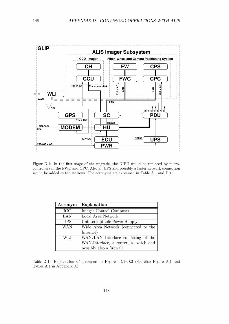
148 APPENDIX D. CONTINUED OPERATIONS WITH ALIS
LANWAN
WLI
MODEMTelephoneline
Ant.
SC
HU
PDU12 4 5 6 8 37
ECUPWR
UPS230/400 V AC
12 V DC
12 V DC
RS232
RS232
Transputer−link
CH
CCU230 V AC
CCD−Imager
FWC
FW CPS
CPC
Filter−Wheel and Camera Positioning System
LAN
230
V A
C
230
V A
C
LAN
ALIS Imager Subsystem
GPS
GLIP
Figure D.1: In the first stage of the upgrade, the NIPU would be replaced by micro-controllers in the FWC and CPC. Also an UPS and possibly a faster network connectionwould be added at the stations. The acronyms are explained in Table A.1 and D.1
Acronym Explanation
ICC Imager Control Computer
LAN Local Area Network
UPS Uninterruptable Power Supply
WAN Wide Area Network (connected to theInternet)
WLI WAN/LAN Interface consisting of theWAN-Interface, a router, a switch andpossibly also a firewall
Table D.1: Explanation of acronyms in Figures D.1–D.2 (See also Figure A.1 andTables A.1 in Appendix A)
148
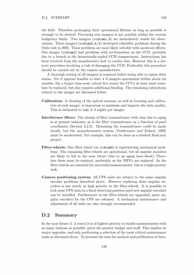
D.2. SUMMARY 149
the field. Therefore prolonging their operational lifetime as long as possible isstrongly to be desired. Procuring new imagers is not possible within the currentbudgetary limits. Two imagers (ccdcam1,6) are immediately usable for obser-vations. Three imagers (ccdcam3,4,5) developed reliability problems during theOulu visit in 2002. These problems are most likely solvable with moderate efforts.One imager (ccdcam2) had problems with ice-formation on the CCD, probablydue to a breach in the hermetically-sealed CCD compartment. Instructions hasbeen received from the manufacturer how to resolve this. However this is a del-icate procedure involving a risk of damaging the CCD. Preferably this procedureshould be carried out by the camera manufacturer.
A thorough testing of all imagers is required before being able to assess theirstatus. Yet it appears feasible to have 4–6 imagers operational within about sixmonths. On a longer time-scale (about five years) the CCUs at least must some-how be replaced, but this requires additional funding. The remaining subsystemsrelated to the imager are discussed below:
Calibration: A cleaning of the optical systems, as well as focusing and calibra-tion of each imager, is important to maintain and improve the data quality.This is estimated to take 2–3 nights per imager.
Interference filters: The change of filter transmittance with time due to agingis at present unknown, as is the filter transmittance as a function of pixelcoordinates (Section 4.2.3). Measuring the transmittance could be madelocally, but the monochromator system [Vaattovaara and Enback , 1993]must be modernised. For example, this can be done as a student final-yearproject.
Filter-wheels: One filter wheel (on ccdcam5) is experiencing mechanical prob-lems. The remaining filter-wheels are operational, but all angular encodersare likely to fail in the near future (due to an aging laser-diode) There-fore these must be replaced, preferably as the NIPUs are replaced. As thefilter-wheels are essential for successful measurements, this is a high-prioritytask.
Camera positioning system: All CPS units are subject to the same angularencoder problems described above. However replacing these angular en-coders is not nearly as high priority as the filter-wheels. It is possible tolock some CPS units in a fixed observing position until new angular encoderscan be installed. Furthermore as the filter-wheels are upgraded, spare an-gular encoders for the CPS are released. A mechanical maintenance andadjustment of all units are also strongly recommended.
D.2 Summary
In the near future (1–2 years) it is of highest priority to enable measurements withas many stations as possible, given the present budget and staff. This implies nomajor upgrades, and only performing a selection of the most critical maintenancetasks as discussed above. To increase the time for analysis and publication of data,
149
150 APPENDIX D. CONTINUED OPERATIONS WITH ALIS
as well as for performing the necessary upgrades and maintenance, it might bean option to increase the student involvement in the observations, as well as insome software development and data-analysis.
The fate (i.e. funding) of ALIS in a longer perspective is directly dependenton what actions are taken in the upcoming 1–3 years. A stable core-group withthorough scientific and technical experience from ALIS operations is withoutdoubt the most critical component.
D.2.1 A longer perspective
Given a sustained and increased funding in the future, upgrading (or replacing)the imagers is required in a longer perspective. Also all obsolete systems atthe stations need to be replaced. The next step would probably be to expandALIS towards Tromsø with station (9) Frihetsli (Figure 2.4 and Table 2.3) andpossibly near the EISCAT site at Ramfjordmoen, as well as equipping the existingstations (7) Kilvo and (8) Nytorp with instruments. For such new stations atentative block-diagram appears in Figure D.2. It must also not be forgotten
WLI
GLIP−LAN
WAN
GLIP−LAN
CCH
CCU
ICC
CCD−Imager
230 V AC
FWC
FW CPS
CPC
Filter−Wheel and Camera Positioning system
230
V A
C
230
V A
C
ALIS Imager Subsystem
PWRECU
UPS
PDUHU
RS232
Ant.
GPSOther
Scientificsubsystems
GLIP
230/400 V AC 230 V AC
Cellphone Antenna
230 V AC
230 V AC
Figure D.2: For future new stations, the SC is replaced by an new HU, which might havea cell-phone interface for emergency operation. The imager is controlled by a dedicatedcomputer, and the dial-up line is replaced by a high-speed Internet connection.
that the GLIPs are capable of housing several other instruments of various types(Section 2.1). Such instruments could include imaging spectrometers, dedicatedcloud cameras, colour imagers for auroral imaging (Appendix C), magnetometers,riometers, ionosondes, etc.
Another issue is that as the stations become networked over permanent Inter-net connections, there will be no need for a dedicated control centre as illustratedin Figure D.3. Given an internationally-standardised set of interfaces, any collec-
150

D.2. SUMMARY 151
alis.irf.se
User Interfaces
EISCAT
httpssh sshhttp
Figure D.3: A decentralised future ALIS: As the ALIS stations will most likely gainpermanent Internet access in the future, the functions of the control centre will be de-centralised to the stations. Connections to other stations, as well as other instruments(exemplified by EISCAT and a satellite) can then also be initiated as required.
tion of instruments could be quickly enrolled into simultaneous observations of aparticular phenomena.
In the future perhaps scientific instruments will be placed on a standardisedGeneral Instrument Platform (GIP), which can be either ground-based, airborne,or placed on a spacecraft. Networks of such GIPs could then be spontaneouslycreated, configured and controlled for specific scientific studies. Developing suchideas might enhance the availability and usage of the existing plethora of scientificinstrumentation, in the same way as the world-wide-web enhanced simplifiedInternet usage.
151

152 APPENDIX D. CONTINUED OPERATIONS WITH ALIS
152
BIBLIOGRAPHY 153
Bibliography
Adeishvili, T. G., A. V. Gurevich, S. B. Lyakhov, G. G. Managadze, G. M. Milikh,and I. S. Shlyuger, Ionospheric emisson caused by an intense radio wave, Sov.J. Plasma Phys., 4 , 721–726, 1978.
Alpatov, V., A. Steen, and U. Brandstrom, Fractal analysis of the ALIS auroralimages, 1996a, (draft manuscript).
Alpatov, V. A., A. A. Matveev, C.-F. Enell, B. Gustavsson, and U. Brandstrom,Investigations of the polar atmosphere with the use of dynamical characteristicsof the processes and self-organizing neural networks on ground-based multi-position optical observations, in Proceedings of the EGS General Assembly ,2000.
Alpatov, V. V., U. Brandstrom, A. Steen, and B. Gustavsson, Fractal analysisof auroral images from ALIS, (poster presentation), 1996b, The third interna-tional substorm conference (ICS3), Paris, France.
Andersson, L., Acceleration processes in auroral region, Ph.D. thesis, SwedishInstitute of Space Physics, 2000, (IRF Scientific Report 270 ISBN: 91-7191-914-7).
Anger, C. D., S. K. Babey, A. L. Broadfoot, R. G. Brown, L. L. Cogger, R. Gat-tinger, J. W. Haslett, R. A. King, D. J. McEwen, J. S. Murphree, E. H.Richardson, B. R. Sandel, K. Smith, and A. Vallance Jones, An ultravioletauroral imager for the Viking spacecraft, Geophys. Res. Lett., 14 , 387–390,1987.
Angstrom, A. J., Recherches sur le Spectre Solaire, W. Schultz, Uppsala, 1868.
Angstrom, A. J., Spectrum des Nordlichts, Pogg. Ann., 137 , 161–163, 1869.
Aristotle, Meteorologica, vol. I, chap. 5, (ancient text), ca. 340 B.C.
Aruliah, A. L., A. D. Farmer, D. Rees, and U. Brandstrom, The seasonal beha-viour of high-latitude thermospheric winds and ion velocities observed over onesolar cycle, J. Geophys. Res., 101 , 15,701–15,711, 1996.
Aso, T., M. A. Hashimoto, T. Ono, and M. Ejiri, On the analysis of aurora stereoobservations, J. Geomag. Geoelectr., 42 , 579–595, 1990.
153

154 BIBLIOGRAPHY
Aso, T., M. Ejiri, H. Miyaoka, T. Ono, T. Hashimoto, T. Yabu, and M. Abe,Aurora stereo observations in Iceland, in Proc. NIPR Symposium on UpperAtmos. Phys., vol. 6, pp. 1–14, National Institute of Polar Research, 1993.
Aso, T., M. Ejiri, H. Miyaoka, T. Ono, Y. Tetsuro, K. Muguruma, T. Hashimoto,and M. Abe, Aurora stereo observation in Iceland and its tomography analysis,Trans. Inst. Electronics Communication Engineers, J77-DII , 69–78, 1994, (inJapanese).
Aso, T., M. Ejiri, A. Urashima, H. Miayoka, A. Steen, U. Brandstrom, andB. Gustavsson, First results from auroral tomography from ALIS-Japan multi-station observations in March 1995, Earth Planets Space, 50 , 81–86, 1998a.
Aso, T., M. Ejiri, A. Urashima, H. Miyaoka, A. Steen, U. Brandstrom, andB. Gustavsson, Auroral tomography analysis of a folded arc observed at theALIS-JAPAN multi-station campaign on March 26, 1995, in Proceedings of theNIPR Symposium on upper atmosphere Physics, vol. 11, pp. 1–10, NationalInstitute of Polar Research, Tokyo, 1998b.
Aso, T., A. Steen, U. Brandstrom, B. Gustavsson, A. Urashima, and M. Ejiri,ALIS — a state of the art optical observation network for the exploration ofpolar atmospheric processes, Adv. Space Res., 26 , 917–924, 2000.
AstroCam Ltd., 4400 Programmer’s reference manual , AstroCam Ltd., 1995.
AstroMed Ltd., 4400 Programmer’s reference manual , AstroMed Ltd., 1993.
Backlund, V., Uber die Technik der simultanen Telefilmsplanigraphie, Acta Ra-diol. Suppl., 137 , 1956, (PhD Thesis).
Baker, D. J., and G. J. Romick, The Rayleigh interpretation of the unit in termsof column emission rate or apparent radiance expressed in SI units, AppliedOptics, 15 , 1966–1968, 1976.
Barmore, F. E., High resolution observations of the 6300 A oxygen line in theday airglow, Planet Space Sci., 25 , 185–191, 1977.
Baschin, O., Die ersten Nordlichtphotographien etc., Met. Z., 17 , 1900.
Bens, A. R., L. L. Cogger, and G. G. Shepherd, Upper atmospheric temperaturesfrom Doppler line-widths — Observation of the OI dayglow emission at 6300 A,Planet Space Sci., 13 , 551–563, 1965.
Bernhardt, P. A., C. A. Tepley, and L. M. Duncan, Airglow enhancements asso-ciated with plasma cavities formed during ionospheric heating experiments, J.Geophys. Res., 94 , 9071–9092, 1989.
Bernhardt, P. A., W. A. Scales, S. M. Grach, A. N. Keroshtin, D. S. Kotik, andS. V. Polyakov, Excitation of artificial airglow by high power radio waves fromthe SURA ionospheric heating facility, Geophys. Res. Lett., 18 , 1477–1480,1991.
154
BIBLIOGRAPHY 155
Birkeland, K., The Norwegian aurora polaris expedition 1902–1903. Volume I Onthe cause of magnetic storms and the origin of terrestrial magnetism. Firstsection, vol. 1, A. W. Brøggers bogtryckeri, Christiania (Oslo), Norway, 1908.
Birkeland, K., The Norwegian aurora polaris expedition 1902–1903. Volume I Onthe cause of magnetic storms and the origin of terrestrial magnetism. Secondsection, vol. 1, A. W. Brøggers bogtryckeri, Christiania (Oslo), Norway, 1913.
Brandy, J. H., and J. E. Hill, Rapid determination of auroral heights, Canad. J.Phys., 42 , 1813–1819, 1964.
Brown, N. B., T. N. Davis, T. J. Hallinan, and H. C. Stenbaek-Nielsen, Altitudeof pulsating aurora determined by a new instrumental technique, Geophys. Res.Lett., 3 , 403–404, 1976.
Brandstrom, B. U. E., T. B. Leyser, A. Steen, M. T. Rietveld, B. Gustavsson,T. Aso, and M. Ejiri, Unambigous evidence of HF pump-enhanced airglow,Geophys. Res. Lett., 26 , 3561–3564, 1999.
Brandstrom, U., Reduction of CCD images from ALIS, ALIS internal note, 2000,(Intended for CCD-course).
Brandstrom, U., ALIS, a brief technical summary of the current situation, ALISinternal note, 2001a.
Brandstrom, U., ALIS stangt for sasongen, email to alis [email protected] 2001-04-11,2001b, (in Swedish).
Brandstrom, U., and A. Steen, Report on the ALIS project, in Proc. 19th AnnualEuropean meeting on atmospheric studies by optical methods, Kiruna, Sweden,edited by A. Steen, pp. 310–321, Swedish Institute of Space Physics, Kiruna,Sweden, 1992, IRF Scientific Report 209.
Brandstrom, U., A. Steen, B. Gustavsson, L. Andersson, I. Haggstrom, A. West-man, A. Pellinen-Wannberg, T. Aso, K. Kaila, C. W. Carlson, D. Klumpar,and C. Catell, Preliminary results from coordinated measurements by FASTand groundbased optical and radar facilities, in Northern Scandinavia, duringactive auroral conditions, in Proceedings of the 24th annual European Meetingon Atmospheric Studies by Optical Methods, pp. 41–46, Sentraltrykkeriet A/SBodø, 1997a, ISBN 82-994583-0-7.
Brandstrom, U., A. Steen, B. Gustavsson, D. Rees, and M. J. Harris, Prelimin-ary results from a comparision of observations of thermospheric neutral windpatterns and auroral emissions, in Proceedings of the 24th annual EuropeanMeeting on Atmospheric Studies by Optical Methods, pp. 37–40, Sentraltryk-keriet A/S Bodø, 1997b, ISBN 82-994583-0-7.
Brandstrom, U., A. Steen, P. Rydesater, B. Gustavsson, and T. Aso, ALIS, amulti station imaging facility with possibilities of future VI applications, inNinth workshop on Virtual Intelligence / Dynamic neural networks, edited by
155
156 BIBLIOGRAPHY
M. L. P. Thomas Lindbladh and J. Kinser, vol. 3728, pp. 108–114, Royal Insti-tute of Technology, Stockholm, Sweden, The International Society for OpticalEngineering, 1998, ISBN 0-8194-3202-4.
Brandstrom, U., B. Gustavsson, A. Steen, and A. Pellinen-Wannberg, ALIS (Au-roral Large Imaging System) used for optical observations of the meteor impactprocess, in Proceedings of the Meteoroids 2001 Conference, edited by B. Warm-bein, vol. SP-495, pp. 331–336, European Space Agency, 2001a, ISBN 92-9092-805-0.
Brandstrom, U., T. Lovgren, A. Mostrom, C.-F. Enell, B. Gustavsson, T. Aso,M. Ejiri, A. Steen, and P. Rydesater, Brief report on ALIS (Auroral LargeImaging System), a new all-sky camera in Kiruna and auroral imaging using amini-DV camcorder, in Proc. of 28th Annual European Meeting on AtmosphericStudies by Optical Methods, Sodankyla Geophysical Observatory, 2001b, (inpress).
Carlson, C. W., The Fast Auroral SnapshoT explorer, EOS, Transactions, Amer-ican Geophysical Union, 73 , 1992.
Carlsson, H. C., V. B. Wickwar, and G. P. Mantas, Observations of suprathermalelectrons accelerated by HF-excited instabilities, J. Atmos. Terr. Phys., 44 ,1089–1100, 1982.
Celsius, A., Observationes de lumine boreali , Norimbergae, 1733.
Ceplecha, Z., and J. Rajchl, The meteor spectrum with dispersion from 11 to 38A/mm, Publishing House of the Czechoslovak Academy of Sciences, 14 , 29–47,1963, (Available from the NASA Astrophysics Data System).
Chamberlain, J. W., Physics of the aurora and airglow , Classics in geophysics,AGU (American Geophysical Union), 1995, (A reprint of the original workfrom 1961).
Cocks, T. D., D. F. Creighton, and F. Jacka, Application of a dual Fabry-Perotspectrometer for daytime airglow studies, J. Atmos. Terr. Phys., 42 , 499–511,1980.
Conde, M., and F. Jacka, Analysis of day-time observations of the 630 nm thermo-spheric emission over Mawson, Antarctica, ANARE Res. notes, 69 , 125–138,1989.
Conde, M. P., P. Greet, and F. Jacka, The Ring effect in the sodium D2Fraunhofer line of day skylight over Mawson, Antarctica, J. Geophys. Res.,97 , 11,561–11,565, 1992.
Cormac, A. M., Representation of a function by its line integrals, with someradiological applications, I, J. Appl. Phys., 34 , 2722–2727, 1963a.
Cormac, A. M., Representation of a function by its line integrals, with someradiological applications, II, J. Appl. Phys., 35 , 2908–2913, 1963b.
156
BIBLIOGRAPHY 157
Crutzen, P. J., and F. Arnold, Nitric acid cloud formation in the cold Antarcticstratosphere: a major cause for the springtime ”ozone hole”, Nature, 324 ,651–655, 1986.
Csorba, I., Image Tubes, Howard Sams, Indianapolis, Indiana, 1985.
Davis, T. N., and G. T. Hicks, Television cinemaphotography of Auroras andpreliminary measurements of auroral velocities, J. Geophys. Res., 69 , 1931,1964.
de Mairan, J. J. D., Traite Physique et Historique de l’Aurore Boreale, ImprimerieRoyale, Paris, 1733, (2ns ed., 1754).
Delbouille, L. G., L. G. Roland, and L. Neven, Photometric atlas of the solarspectrum from 3000 to 10000 A, Institute d’Astrophysique de l’Universite deLiege, Cointe-Ougre, Belgium, 1973.
Djuth, F. T., P. A. Bernhardt, C. A. Tepley, J. A. Gardner, M. C. Keley, A. L.Broadfoot, L. M. Kagan, M. P. Sulzer, J. H. Elder, C. Selcher, B. Isham,C. Brown, and H. C. Carlson, Large airglow enhancements produced via wave-plasma interactions in sporadic E, Geophys. Res. Lett., 26 , 1557–1560, 1999.
Dressler, R. A., J. A. Gardener, R. H. Salter, and E. Murad, Luminescence meas-urements of Ar+ + H2O and N+
2 + H2O suprathermal charge transfer collisions:Product state distribution from H2O
+A2A1−X2B1 analysis, J. Chem. Phys.,96 , 1062–1076, 1992.
Eather, R. H., Majestic lights the aurora in science, history and the arts, AGU(American Geophysical Union), Washington D.C., 1980, ISBN: 0-87590-215-4.
Eather, R. H., Low light level imaging design, Tech. rep., Air Force Geophysicslaboratory, USAF, Hanscom AFB, Massachusetts USA, 1982, AFGL-TR-82-0308.
Eide, A. J., V. Becanovic, U. Brandstrom, C. Holmstrom, M. Larsson, I. M.Lillesand, T. Lindblad, C. S. Lindsey, A. Steen, and J. Waldemark, Pulsecoupled neural network pre-processing of aurora images, in AI Applications inSolar Terrestial Physics, vol. WPP-148, pp. 201–205, European Space Agency,1997.
Ejiri, M., M. Okada, M. Tsutsumi, M. Taguchi, and S. Okano, All sky imagerobservation of aurora and airglow at south pole station : Initial results, inProceedings of the 25th annual European Meeting on Atmospheric Studies byOptical Methods, Granada, Spain, pp. 54–57, 1998.
Ejiri, M., T. Aso, M. Okada, M. Tsutsumi, M. Taguchi, N. Sato, and S. Okano,Japanese research project on Arctic and Antarctic observations of the middleatmosphere, Adv. Space Res., 24 , 1689–1692, 1999.
Elvey, C. T., and W. Stoffregen, Auroral photography by all-sky camera, Ann.IGY., 5 , 117–151, 1957.
157
158 BIBLIOGRAPHY
Enell, C.-F., Optical studies of polar stratospheric clouds and related phenomena,Ph.D. thesis, Swedish Institute of Space Physics, Kiruna, Sweden, 2002, (IRFScientific Report 278), ISBN: 91-7305-307-4.
Enell, C.-F., B. Gustavsson, A. Steen, U. Brandstrom, P. Rydesater, P. Johans-son, T. Wagner, U. Friess, K. Pfeilsticker, and U. Platt, Optical studies of polarstratospheric clouds, in Proceedings of SPIE, Satellite remote sensing of cloudsand the atmosphere IV , edited by J. E. Russell, vol. 3867, pp. 290–297, TheInternational Society for Optical Engineering, 1999a.
Enell, C.-F., A. Steen, B. Gustavsson, U. Brandstrom, P. Johansson, T. Wagner,U. Frieß, K. Pfeilsticker, and U. Platt, Studies of polar stratospheric cloudsoccurence at Kiruna, in XXV annual European Meeting on Atmospheric Stud-ies by Optical Methods, pp. 122–126, Instituto de Astrofısica de Andalucia,Granada, Spain, 1999b.
Enell, C.-F., A. Steen, B. Gustavsson, U. Brandstrom, P. Johansson, T. Wagner,U. Frieß, K. Pfeilsticker, U. Platt, and K.-H. Fricke, Detection of polar strato-spheric clouds at Kiruna, in Air pollution report 69, Mesoscale processes in thestratosphere, edited by K. S. Carslaw and G. T. Amanatidis, vol. 18912, pp.65–68, Office for Official Publications of the European Communities, EuropeanCommission, Luxembourg, 1999c, ISBN 92-828-4629-6.
Enell, C.-F., B. Gustavsson, A. Steen, U. Brandstrom, and P. Rydesater, Multi-static imaging and optical modelling of nacreous clouds, Phys. Chem. Earth,25 , 451–457, 2000.
Enell, C.-F., U. Brandstrom, B. Gustavsson, S. Kirkwood, K. Stebel, andA. Steen, Case studies of the development of polar stratospheric clouds us-ing bistatic imaging, Ann. Geophys., 2003, (in press).
Frey, S., H. U. Frey, D. J. Carr, O. H. Bauer, and G. Haerendel, Auroral emissionprofiles extracted from three-dimensionally reconstructed arcs., J. Geophys.Res., 101 , 21,731–21,741, 1996.
Galand, M., Special section: Proton precipitation into the atmosphere, J. Geo-phys. Res., 106 , 1–178, 2001.
Galperin, Y. I., Multiple scales in auroral plasmas, J. Atmos. Solar and Terr.Phys., 64 , 211–229, 2001.
Gardner, J. A., A. L. Broadfoot, W. J. McNeil, S. T. Lai, and E. Murad, Analysisof the GLO-1 observations of meteoric metals in the thermosphere, J. Atmos.Terr. Phys., 61 , 545–562, 1999.
Gartlein, C. W., Unlocking secrets of the northern lights, Nat. Geograph. Mag.,p. 673, 1947.
Gassendi, P., De vita Pereskii, Anno 1621 , Edit. Hag. Com., 1651.
Gilbert, P., Iterative methods for the three-dimensional reconstruction of an ob-ject from projections, J. Theor. Boil., 36 , 105–117, 1972.
158

BIBLIOGRAPHY 159
Gurevich, A. V., and G. M. Milikh, Artificial airglow due to modifications of theionosphere by powerful radio waves, J. Geophys. Res., 102 , 389–394, 1997.
Gurevich, A. V., Y. S. Dimant, G. M. Milikh, and V. V. Va’skov, Multiple ac-celeration of electrons in the regions of high power radio-wave reflection in theionosphere, J. Atmos. Terr. Phys., 47 , 1057–1070, 1985.
Gustavsson, B., A study of feasible tomographic inversion techniques for ALIS,Tech. Rep. 039 , Swedish Institute of Space Physics, Kiruna, Sweden, 1992,ISSN 0284-1738.
Gustavsson, B., Private communication, 1997.
Gustavsson, B., Tomographic inversion for ALIS noise and resolution, J. Geophys.Res., 103 , 26,621–26,632, 1998.
Gustavsson, B., Three Dimensional Imaging of Aurora and Airglow,, Ph.D. thesis,Swedish Institute of Space Physics, Kiruna, Sweden, 2000, (IRF Scientific Re-port 267), ISBN: 91-7191-878-7.
Gustavsson, B., Private communication, 2003.
Gustavsson, B., T. Sergienko, M. T. Rietveld, F. Honary, A. Steen, B. U. E.Brandstrom, T. B. Leyser, A. L. Aruliah, T. Aso, and M. Ejiri, First tomo-graphic estimate of volume distribution of enhanced airglow emission causedby HF pumping, J. Geophys. Res., 106 , 29,105–29,123, 2001a.
Gustavsson, B., A. Steen, T. Sergienko, and B. U. E. Brandstrom, Estimateof auroral electron spectra, the power of ground-based multi-station opticalmeasurements, Phys. Chem. Earth, 26 , 189–194, 2001b.
Gustavsson, B., B. U. E. Brandstrom, A. Steen, T. Sergienko, T. B. Leyser,M. T. Rietveld, T. Aso, and M. Ejiri, Nearly simultaneous images of HF-pumpenhanced airglow at 6300 A and 5577 A, Geophys. Res. Lett., 29 , 2003, paperNo. 10.1029/2002GL015350.
Hallinan, T. J., H. C. Stenbaek-Nielsen, and C. S. Deehr, Enhanced aurora, J.Geophys. Res., 90 , 8461–8475, 1985.
Hammarskjold, D., Vagmarken, Albert Bonniers Forlag AB, 1963, (In Swedish,reprinted 1999 ISBN:9100571121).
Hammarskjold, D., Markings, Knopf, New York, 1964, (transl. by Leif Sjobergand W. H. Auden, ISBN: 039443532X).
Haslett, J. C., and L. R. Megill, A model of the enhanced airglow excited byRF-radiation, Radio Sci., 9 , 1005–1019, 1974.
Hecht, J. H., A. B. Christensen, D. J. Strickland, and R. R. Meier, Deducingcomposition and incident electron spectra from ground-based auroral opticalmeasurements: Variation in oxygen density, J. Geophys. Res., 94 , 13,553–13,563, 1989.
159
160 BIBLIOGRAPHY
Hedin, M., I. Haggstrom, A. Pellinen-Wannberg, I. Haggstrom, L. Andersson,U. Brandstrom, B. Gustavsson, A. Steen, A. Westman, G. Wannberg, T. vanEyken, T. Aso, C. Cattell, C. W. Carlson, and D. Klumpar, Trough observa-tions with the EISCAT radars, ALIS auroral imaging system and FAST satel-lite, in Proceedings of RadioVetenskap och Kommunikation 99 , edited by J.-O.Gustavsson, vol. 1, pp. 113–117, Hogskolan i Karlskrona/Ronneby, Karlskrona,Sweden, 1999, ISBN 91-630-8156-3.
Hedin, M., I. Haggstrom, A. Pellinen-Wannberg, I. Haggstrom, L. Andersson,U. Brandstrom, B. Gustavsson, A. Steen, A. Westman, G. Wannberg, T. vanEyken, T. Aso, C. Cattell, C. W. Carlson, and D. Klumpar, 3-D extent of themain ionospheric trough —a case study, Adv. Polar Upper Atmos. Res., 14 ,157–162, 2000.
Henriksen, K., W. Stoffregen, B. Lybekk, and A. Steen, Photometer and spec-trometer search of the oxygen green and red lines during artificial ionosphericheating in the auroral zones, Ann. Geophys., 2 , 73–76, 1984.
Hernandez, G., Fabry-Perot Interferometers, Cambridge University Press, 1986,ISBN: 0-521-32238-3.
Hertel, R. J., Signal and noise properties of proximity focused image tubes, inUltrahigh Speed and High Speed Photography, Photonics and Videography , ed-ited by G. L. Stradling, vol. 1155, pp. 332–343, The International Society forOptical Engineering, 1989.
Hesstvedt, E., On the physics of mother of pearl clouds, Geofysiske Publikasjoner ,XXI , 1–32, 1960.
Holst, G. C., CCD arrays, cameras and displays, 2nd ed., The InternationalSociety for Optical Engineering, 1998, ISBN: 0-8194-2853-1.
Høymork, S. H., ed., Sensors and Instruments for Space Exploration, chap. 6.Measurements by optical methods, pp. 71–119, 2nd ed., Swedish Institute ofSpace Physics, Kiruna, 2000.
Hunten, D. M., F. E. Roach, and J. W. Chamberlain, A photometric unit for theaurora and airglow, J. Atmos. Terr. Phys., 8 , 345–346, 1956.
Hypponen, M., R. Pellinen, C. Sucksdorff, and R. Torniainen, Digital all-skycamera, Tech. Rep. 9 , Finnish Meteorological Institute, Helsinki, 1974.
Hoffner, J., and U. von Zahn, The 1996 Leonid shower as studied with a potassiumlidar: Observations and inferred meteoroid sizes, J. Geophys. Res., 104 , 2633–2643, 1999.
Ivanov, V. E., and T. I. Sergienko, Interaction of the auroral electrons with theatmospheric gases. (the Monte-Carlo modelling), 1992, Nakua, St. Petersburg,1992.
Janesick, J. R., T. Elliott, S. Collins, M. M. Blouke, and J. Freeman, Scientificcharge-coupled devices, Optical Engineering , 26 , 692–714, 1987.
160
BIBLIOGRAPHY 161
Johansson, H., Station software for ALIS, IRF Tech. Report 036 , Swedish Insti-tute of Space Physics, 1991, ISSN 0284-1738.
Jones, A. R. V., R. L. Gattinger, F. Creutzberg, F. R. Harris, A. G. McNamara,A. W. Yau, E. J. Llewellyn, D. Lummerzheim, M. H. Rees, I. C. McDade,and J. Margot, The ARIES auroral modelling campaign: Characterization andmodelling of an evening auroral arc observed from a rocket and a ground-basedline of meridian scanners, Planet Space Sci., 39 , 1677–1705, 1991.
Jones, A. V., Aurora, vol. 9 of Geophysics and astrophysics monographs, D. ReidelPublishing Company, 1974, ISBN: 90-277-0272-1.
Kaila, K., Optical instrumentation of Oulu, http://spaceweb.oulu.fi/
projects/optical and Private communication, 2003a.
Kaila, K., Private communication, 2003b, data analysis and publication in pro-gress.
Kaila, K., Private communication, 2003c, (See also http://spaceweb.oulu.fi/
projects/optical).
Kaila, K. U., An iterative method for calculating the altitudes and positions ofauroras along the arc, Planet. Space Sci., 35 , 245–258, 1987.
Kaila, K. U., and H. J. Holma, Absolute calibration of photometer, Phys. Chem.Earth, B(25), 467–470, 2000.
Keo Consultants, Kiruna telecentric lens systems, 1994, vendor-provided docu-mentation.
Keo Consultants, Telecentric lens for Kyoto university, 1997, vendor-provideddocumentation.
Kinser, J. M., and T. Lindblad, Detection of microcalcifications by cortical stimu-lation, in Proceedings EANN’97 Neural networks in engineering systems, editedby A. Bulsari and S. Kallio, pp. 203–206, 1997, ISBN: 952908667-9.
Kosch, M. J., T. Rietveld, M., S. A, and T. Hagfors, HF-Induced Airglow: DoublePatches, Phys. Chem. Earth, 25 , 475–581, 2000a.
Kosch, M. J., T. Rietveld, M., T. Hagfors, and T. B. Leyser, High-latitude HF-induced airglow displaced equatorward of the pump beam, Geophys. Res. Lett.,27 , 2817–2820, 2000b.
Kosch, M. J., M. T. Rietveld, A. J. Kavanagh, C. Davis, T. Yeoman, F. Honary,and T. Hagfors, High-latitude pump-induced optical emissions for frequenciesclose to th third electron gyro-harmonic, Geophys. Res. Lett., 29 , 27–1–274,2002a.
Kosch, M. J., M. T. Rietveld, T. Yeoman, K. Cierpka, and T. Hagfors, The high-latitude artificial aurora of 21 February 1999: An analysis, Adv. Polar UpperAtmos. Res., 2002b, (in press).
161
162 BIBLIOGRAPHY
Labsphere, A guide to integrating sphere theory and applications, Labsphere,1997.
Lance, C., and R. H. Eather, High frequency active auroral research pro-gram (HAARP) imager, Tech. rep., Air Force Geophysics laboratory, USAF,Hanscom AFB, Massachusetts USA, 1993, PL-TR-93-2219.
Lauche, H., and O. Widell, Intercalibration of low light level sources, letter fromHans Lauche, 2000a.
Lauche, H., and O. Widell, Intercalibration of low light level sources, in Proc.of 27th Annual European Meeting on Atmospheric Studies by Optical Methods,Stockholm, Sweden, Meteorological institution, Stockholm university, Sweden,2000b.
Leyser, T. B., Parametric interactions between upper hybrid and lower hybridwaves in heating experiments, Geophys. Res. Lett., 18 , 408–411, 1991.
Leyser, T. B., and B. Gustavsson, Private communication, 2003.
Leyser, T. B., B. Gustavsson, B. U. E. Brandstrom, F. H. A. Steen, T. A.M. T. Rietveld, and M. Ejiri, Simultaneous measurements of high-frequencypump-enhanced airglow and ionospheric temperatures at auroral latitudes,Adv. Polar Upper Atmos. Res., 14 , 1–11, 2000.
Leyser, T. B., B. U. E. Brandstrom, B. Gustavsson, T. Sergienko, and M. T.Rietveld, Enhanced airglow by high frequency electromagnetic pumping withthe EISCAT heating facility and observed by the multi-station auroral largeimaging system ALIS, in URSI , URSI, 2002, paper 815, 2002.
Lodin, H., The value of tomography in examination of the intrapulmonary bron-chi, Acta Radiol. Suppl., 101 , 1935.
Love, S. G., and D. E. Brownlee, A direct measurement of the terrestial massaccretion rate of cosmic dust, Science, 262 , 550–553, 1993.
Macleod, H. A., Thin-film optical filters, Macmillan, New York, 1986, ISBN:0-02-948110-4.
Mantas, G. P., Large 6300 A airglow intensity enhancements observed in iono-sphere heating experiments are excited by thermal electrons, J. Geophys. Res.,99 , 8993, 1994.
Mantas, G. P., and H. C. Carlson, Reinterpretation of the 6300 A airglow en-hancements observed in the ionosphere heating experiments based on analysisof Platteville Colorado, J. Geophys. Res., 101 , 195–209, 1996.
Massey, P., A User’s guide to CCD Reductions with IRAF , National OpticalAstronomy Observatory, 1992, http://iraf.noao.edu/docs.
McDade, I. C., and E. J. Llewellyn, Satellite airglow limb tomography: Meth-ods for recovering structured emission rates in the mesospheric airglow layer,Canad. J. Phys., 71 , 552–563, 1994.
162
BIBLIOGRAPHY 163
McNaught, R. H., and D. J. Asher, Variation of Leonid maximum times withlocation of observer, Meteorit. Planet. Sci., 34 , 975–978, 1999.
McNeil, W. J., E. Murad, and S. T. Lai, Comprehensive model for the atmo-spheric sodium layer, J. Geophys. Res., 100 , 16,847–16,855, 1995.
McNeil, W. J., S. T. Lai, and E. Murad, Models of thermospheric sodium, calciumand magnesium at the magnetic equator, Adv. Space Res., 21 , 863–866, 1998.
McNeil, W. J., R. A. Dressler, and E. Murad, Impact of a major meteor storm onearth’s ionosphere: A modeling study, J. Geophys. Res., 106 , 10,447–10,465,2001.
McWhirter, I., Imaging photon detectors and their use with single and multiplefabry-perot etalon systems for atmospheric wind measurements, Ph.D. thesis,University College London, London, 1993.
Meier, R. R., D. J. Strickland, J. H. Hecht, and A. B. Christensen, Deducingcomposition and incident electron spectra from ground-based auroral opticalmeasurements: a study of auroral red line processes, J. Geophys. Res., 94 ,13,541–13,552, 1989.
Mills, D. L., Network time protocol (version 3) specification, implementationand analysis, Request for Comments: 1305, 1992, ftp://ftp.rfc-editor.org/in-notes/rfc1305.txt.
Mohn, H., Perlemorskyer, in Christiania Videnskabs-Selskabs Forhandlinger ,vol. 2, A. W. Brøggers bogtryckeri, Christiania (Oslo), Norway, 1893.
Na, H., and H. Lee, Orthogonal decomposition technique for ionospheric tomo-graphy, Int. J. Imaging Syst. Technol., 3 , 354–365, 1991.
NASA, Definition of the Flexible Image Transport System (FITS),NASA/Science Office of Standards and Technology, Code 633.2, NASAGoddard Space Flight Center, Greenbelt MD, USA, 1999, nOST 100-2.0,http://fits.gsfc.nasa.gov/fits documentation.html.
Nilsson, L., OPERA operations program for ALIS version 1.0, Internal Note 024 ,Swedish Institute of Space Physics, Kiruna, Sweden, 1994.
Nilsson, L., and B. Nystrom, OPERA operations program for ALIS version 1.0,IRF Tech. Rep. 037 , Swedish Institute of Space Physics, Kiruna, Sweden, 1992,ISSN 0284-1738.
Noxon, J. F., and R. M. Goody, Observations of day airglow, J. Atmos. Sci., 19 ,342–343, 1962.
Okano, S., S. Takeshita, and M. Taguchi, Absolute calibration system at NIPRfor aurora/airglow measurements using an 1.9 m integrating sphere, in Proceed-ings of the 24th annual European Meeting on Atmospheric Studies by OpticalMethods, Sentraltrykkeriet A/S Bodø, 1997, ISBN: 82-994583-0-7.
163

164 BIBLIOGRAPHY
Pedersen, and Carlson, First observations of HF heater-produced airglow at theHigh Frequency Active Auroral Research Program facility: Thermal excitationand spatial structuring, Radio Sci., 36 , 1013–1026, 2001.
Pellinen, R., and K. Kaila, Optical groundbased network, in Proc. of the Clusterworkshop, Svalbard, Norway 16–19 Sept., pp. 147–158, European Space AgencyPublications Division, 1991, (ESA SP-330).
Pellinen-Wannberg, A., E. Murad, B. Gustavsson, U. Brandstrom, C.-F. Enell,C. Roth, I. P. Williams, and A. Steen, Water in Leonid meteor trails, (inpreparation), 2003.
Perkins, F. W., and P. K. Kaw, On the role of plasma instabilities in ionosphericheating by radio waves, J. Geophys. Res., 76 , 282–284, 1971.
Pliny, Historiae Naturalis, vol. II, chap. 27,33, (ancient text), ca. 77.
Pountain, D., The transputer strikes back, Byte, pp. 265–275, 1991.
Preston, T. J., 4400 Quad CCD Camera controller user guide. System descriptionand operations manual , AstroMed Ltd., Cambridge, 1993.
Preston, T. J., 4400 Quad CCD Camera controller user guide for motherboard is-sue B. System description and operations manual , AstroCam Ltd., Cambridge,1995.
Puccio, W., Private communication, 2002.
Pudovkin, M. I., A. Steen, and U. Brandstrom, Vorticity in the magnetosphericplasma and its signature in the aurora dynamics., Space Science Rev., 80 ,411–444, 1997.
Pudovkin, M. I., A. Steen, N. V. Nikolaev, O. I. Kornilov, U. Brandstrom,B. Gustavsson, and P. Rydesater, Automatic recognition of auroral forms, inNinth workshop on Virtual Intelligence / Dynamic neural networks, edited byM. L. P. Thomas Lindbladh and J. Kinser, vol. 3728, pp. 121–127, Royal Insti-tute of Technology, Stockholm, Sweden, The International Society for OpticalEngineering, 1998, ISBN 0-8194-3202-4.
Raspopov, O. M., V. A. Dergachev, and E. G. Goos’kova, Ezekiel’s vision:visual evidence of Sterno-Etrussia geomagnetic excursion?, EOS, Transactions,American Geophysical Union, 84 , 77, 2003.
Rayleigh, L., Absolute intensity of the aurora line in the night sky, and thenumber of atomic transitions required to maintain it, Proc. Roy. Soc. London,A129 , 458, 1930.
Rees, D., I. McWhirter, P. B. Hays, and T. Dines, A stable rugged, capacitance-stabilised piezoelectric scanned Fabry-perot etalon, J. Phys. E: Sci. Instrum.,14 , 1320–1325, 1981.
164
BIBLIOGRAPHY 165
Rees, D., M. Vyssogorets, N. P. Meredith, E. Griffin, and Y. Chaxell, The dopplerwind and temperature system for the ALOMAR observatory: Design and initialresults, J. Atmos. Terr. Phys., 58 , 1827–1842, 1996.
Rees, D., R. W. Smith, F. Sigernes, K. Henriksen, U. Brandstrom, W. B. Wick-war, N. D. Lloyd, and M. Harris, Observations of thermospheric wind patternsin the vicinity of the polar cusp from a doppler imaging system, in Proceed-ings of the 24th annual European Meeting on Atmospheric Studies by OpticalMethods, Sentraltrykkeriet A/S Bodø, 1997, ISBN: 82-994583-0-7.
Rees, D., U. von Zahn, G. von Cossart, K.-H. Fricke, W. Eriksen, and J. A.McKay, Daytime LIDAR measurements of the stratosphere and mesosphere atthe ALOMAR observatory, Adv. Space Res., 1999, proc. COSPAR meeting,Nagoya, July 1998, accepted.
Rees, D., M. Conde, A. Steen, and U. Brandstrom, The first daytime ground-based optical image of the aurora, Geophys. Res. Lett., 27 , 313–316, 2000.
Rees, M. h., and D. Luckey, Auroral electron energy derived from ratio of spec-troscopic emissions 1. model computations, J. Geophys. Res., 79 , 5181, 1974.
Rietveld, M. T., H. Kohl, H. Kopka, and P. Stubbe, Introduction to ionosphericheating at Tromsø —I. Experimental overview, J. Atmos. Terr. Phys., 55 ,577–599, 1993.
Romick, G. J., and A. E. Belon, The spatial variation of auroral luminosity—II,Planet Space Sci., 15 , 1695–1716, 1967.
Rydesater, P., and B. Gustavsson, Investigation of smooth basis functions andan approximated projection algorithm for faster tomography, Int. J. ImagingSyst. Technol., 11 , 347–354, 2001.
Rydesater, P., Processing of multi-station auroral image data, Lic. thesis, AppliedPhysics and Electronics, Umea University, Umea, Sweden, 2001, ISBN: 91-7305-149-7.
Rydesater, P., A. Steen, U. Brandstrom, and B. Gustavsson, Classifying aurorasusing artificial neural networks, in Ninth workshop on Virtual Intelligence /Dynamic neural networks, edited by M. L. P. Thomas Lindbladh and J. Kinser,vol. 3728, pp. 115–120, Royal Institute of Technology, Stockholm, Sweden, TheInternational Society for Optical Engineering, 1998, ISBN 0-8194-3202-4.
Rydesater, P., B. Gustavsson, U. Brandstrom, and A. Steen, Lossy compressionof scientific images of aurora, in Proc. of 28th Annual European Meeting onAtmospheric Studies by Optical Methods, Sodankyla Geophysical Observatory,2001, (in press).
Scourfield, M. W. J., and N. R. Parsons, Auroral pulsations and flaming — Someinitial results of a cinematographic study using an image intensifier, PlanetSpace Sci., 17 , 1141, 1969.
Seneca, Quaestiones Naturales, vol. I, chap. 14–15, (ancient text), ca. 63.
165

166 BIBLIOGRAPHY
Sergienko, T., Private communication, 2003.
Sergienko, T., B. Gustavsson, A. Steen, U. Brandstrom, M. Rietveld, T. Leyser,and F. Honary, Analysis of excitation of the 630.0 nm airglow during heatingexperiment in Tromsø on February 16, 1999, Phys. Chem. Earth, 25 , 531–535,2000.
Simpson, W., The point-to-point protocol (ppp), Request For Comments: 1661 ,1994, ftp://ftp.rfc-editor.org/in-notes/rfc1661.txt.
Sipler, D. P., and M. A. Biondi, Measurements of O(1D) quenching rates in theF region, J. Geophys. Res., 77 , 6202–6212, 1972.
Siscoe, G. L., A historical footnote on the origin of aurora borealis, EOS, Trans-actions, American Geophysical Union, 59 , 994, 1978.
Siscoe, G. L., S. M. Silverman, and K. D. Siebert, Ezekiel and the Northernlights: Biblical aurora seems plausible, EOS, Transactions, American Geo-physical Union, 83 , 173, 2002.
Solomon, S., R. R. Garcia, F. S. Rowland, and D. J. Wuebbles, On the depletionof Antarctic ozone, Nature, 321 , 755–758, 1986.
Solomon, S. C., P. B. Hays, and V. J. Abreu, Tomographic inversion of satellitephotometry, Applied Optics, 23 , 3409–3414, 1984.
Solomon, S. C., P. B. Hays, and V. J. Abreu, The auroral 6300 A emisson:Observation and modelling, J. Geophys. Res., 93 , 9867–9882, 1988.
Spurny, P., H. Betlem, K. Jobse, P. Koten, and J. van’t Leven, New type of brightLeonid meteors above 130 km, Meteorit. Planet. Sci., 35 , 1109–1115, 2000.
Steen, A., The optical laboratory in Kiruna: A new research facility in the auroralzone, KGI Tech. Report 033 , Kiruna Geophysical Institute, Kiruna, Sweden,Kiruna, Sweden, 1987, ISSN 0349-2672.
Steen, A., Investigations of auroral dynamics, techniques and results, Ph.D.thesis, Swedish Institute of Space Physics, Kiruna, Sweden, 1988a, (KGI Sci-entific Report 1994), ISSN 0984-1703.
Steen, A., An auroral height measuring system designed for real time operation,Rev. Sci. Instrum., 1988b.
Steen, A., An Auroral Large Imaging System in Northern Scandinavia, in Proc.9th Symposium on European rocket and ballon programmes and related research,Lahnstein, FRG , pp. 299–303, European Space Agency, 1989, ESA SP-291.
Steen, A., ed., Auroral Tomography workshop proceedings, IRF Scientific Report213, Swedish Institute of Space Physics, 1993, ISSN 0284-1703.
Steen, A., Application for equipment to an optical calibration facility inkiruna, Funding application to Forskningsradsnamnden (FRN), 1998, (partlyin Swedish, IRF Dnr 238-150/98).
166
BIBLIOGRAPHY 167
Steen, A., and P. N. Collis, High time-resolution imaging of auroral arc deform-ation at substorm onset, Planet. Space Sci., 36 , 715–732, 1988.
Steen, A., P. N. Collis, and I. Haggstrom, On the development of folds in auroralarcs, J. Atmos. Terr. Phys., 50 , 301–313, 1988.
Steen, A., U. Brandstrom, and K. Kaila, A scientific and technical description ofALIS, in Proc. NSSR Annual meeting Bolkesjø, Norway , pp. 153–164, NordicSociety for Space Research, 1990.
Steen, A., U. Brandstrom, and B. Gustavsson, ALIS — a multi station imagingsystem at high latitude with multi disciplinary scientific objectives, in Proceed-ings 13th ESA Symposium on European Rocket and Balloon Programmes andRelated Research, pp. 261–266, ESA, 1997a.
Steen, A., B. Gustavsson, and U. Brandstrom, Temporal variation of 2D altitudedistributions of lee-wave generated polar stratospheric clouds, in Proceedingsof the 4th European symposium of polar stratospheric ozone, 1997b.
Steen, A., B. Gustavsson, U. Brandstrom, T. Aso, and M. Ejiri, OI 846.6 nmauroral imaging, in Proceedings of the 25th annual European Meeting on At-mospheric Studies by Optical Methods, Granada, Spain, pp. 90–95, Institutode Astrofısica de Andalucia, Granada, Spain, 1999a.
Steen, A., B. Gustavsson, C.-F. Enell, and U. Brandstrom, PSC dynamics in-vestigated by multi-station imaging — techniques, results and prospects, inAir pollution research report. Mesoscale processes in the stratosphere, editedby K. Carslaw and G. Amanatidis, vol. 69, pp. 239–242, European Comission,1999b, ISBN 92-828-4629-6.
Stenbaek-Nielsen, H. C., and T. J. Hallinan, Pulsating auroras: Evidence fornon-collisional thermalization of precipitating particles., J. Geophys. Res., 84 ,3257–3271, 1979.
Stoffregen, W., All-sky camera auroral research during the third geophysical year1957–1958, Tellus, 7 , 509–517, 1955.
Stoffregen, W., An all-sky camera for auroral research, description and opera-tional manual, Tech. rep., Uppsala Jonosfarsobservatorium, 1956.
Stoffregen, W., ed., I.G.Y. ASCAPLOTS , vol. XX (part 1) of Annals of theinternational geophysical year , Pergamon Press, Oxford, London, New York,Paris, 1962.
Størmer, C., Bericht uber eine Expedition nach Bossekop etc., Vid. Selsk. Skr.Math. Nat. Kl., 1911, Christiania (Oslo), Norway.
Størmer, C., Photogrammetrishe bestimmung der Hohe von irisierenden Wolken(Perlmutterwolken) am 30. Dezember 1926., Geofysiske Publikasjoner , 5 , 1–8,1930.
Størmer, C., The Polar Aurora, Clarendon Press, Oxford, 1955.
167
168 BIBLIOGRAPHY
Strickland, D. J., R. R. Meier, J. H. Hecht, and A. B. Christensen, Deducingcomposition and incident electron spectra from ground-based auroral opticalmeasurements: theory and results, J. Geophys. Res., 94 , 13,527–13,539, 1994.
Stubbe, P., H. Kopka, H. Lauche, M. T. Rietveld, A. Brekke, O. Holt, T. B. Jones,T. Robinson, A. Hedberg, B. Thide, B. Crochet, and H. J. Lotz, Ionosphericmodification experiments in northern Scandinavia, J. Atmos. Terr. Phys., 44 ,1025–1041, 1982.
Syrjasuo, M., New Finnish all-sky cameras, in Proceedings of the 24th annualEuropean meeting on atmospheric studies by optical methods, pp. 247–251,Sentraltrykkeriet A/S Bodø, 1997, ISBN: 82-994583-0-7.
Syrjasuo, M. T., All-sky camera, (master’s-thesis), Helsinki Univ. of Technology,1996.
Syrjasuo, M. T., Auroral monitoring network: From all-sky camera system toautomated image analysis, (D.Sc.(Tech.)-thesis), Finnish Meteorological Insti-tute, Helsinki, Finland, 2001, Contribution series 32, ISBN: 951-697-551-8.
Theuwissen, A. J. P., Solid-state imaging with charge-coupled devices, vol. 1 ofSolid-state scenece and technology library , Kluwer, 1995.
Tolbert, M. A., Polar clouds and sulfate aerosols, Science, 272 , 1597, 1996.
Toon, O. B., P. Hamill, R. P. Turco, and J. Pinto, Condensation of HNO3 andHCl in the winter polar stratospheres, Geophys. Res. Lett., 13 , 1284–1287,1986.
Torneus, A., GOSSIP a general information panel for ALIS, IRF Tech. Rep. 040 ,Swedish Institute of Space Physics, Kiruna, Sweden, 1992, ISSN 0284-1738.
Torr, M. R., and P. Espy, Intercalibration of instrumentation used in the obser-vation of atmospheric emissions: Second progress report, Tech. Rep. 101 , UtahState University, Center for atmospheric and space sciences, Logan Utah, 1981.
Trondsen, T. S., High spatial and temporal resolution auroral imaging, Ph.D.thesis, University of Tromsø, 1998.
Urashima, A., T. Aso, M. Ejiri, A. Steen, U. Brandstrom, and B. Gustavsson,Camera calibration by integrating sphere for the auroral tomography observa-tion, Adv. Polar Upper Atmos. Res., 13 , 79–88, 1999.
Vaattovaara, M., and J. Enback, Development of a calibration system using amonochromator and an APD, Internal Note 023 , Swedish Institute of SpacePhysics, 1993.
Vegard, L., Photographische Aufnahmen des Nordlichtspektrums mit einem Spec-trographen von grosser Dispersion, Phys. Zhur., 14 , 677–681, 1913.
Vegard, L., and O. Krogness, The position in space of the aurora polaris, inGeofysiske Publikasjoner , vol. 1 of Geofysiske Publikasjoner , pp. 1–170, A. W.Brøggers bogtryckeri, Christiania (Oslo), Norway, 1920.
168
BIBLIOGRAPHY 169
Veklerov, E., and J. Llacer, Feasible images and practical stopping rules for it-erative algorithms im emission tomography, IEEE Trans. Medical Imaging , 8 ,186–193, 1989.
von Zahn, U., M. Gerding, J. Hoffner, W. J. M. Neil, and E. Murad, Fe, Ca andK atom densities in the trails of Leonids and other meteors: Strong evidenceof differential ablation., Meteorit. Planet. Sci., 34 , 1017–1027, 1999.
Waldemark, J., V. Becanovic, U. Brandstrom, C. Holmstrom, M. Larsson,T. Lindblad, C. S. Lindsay, and A. Steen, Investigation of useful image prepro-cessing for analysis of aurora images, in Proceedings EANN , 1997.
Wannberg, G., The G2-system and general purpose alternating code experimentsfor EISCAT, J. Atmos. Terr. Phys., 55 , 543–557, 1993.
Weinbren, M., A manual of tomography , H. K. Lewis & Co., 1946.
Weinstock, J., Theory of enhanced airglow during ionospheric modifications, J.Geophys. Res., 80 , 4331, 1975.
Weinstock, J., and B. Bezzerides, Theory of electron acceleration during para-metric instabilities, Phys. Rev. Lett., 32 , 754–758, 1974.
Widell, O., and H. Henricson, Intercalibration of low light level sources, in Proc.of 28th Annual European Meeting on Atmospheric Studies by Optical Methods,Oulu, Finland , Sodankyla Geophysical Observatory, 2001, (in press).
Wilcke, J. C., Tal om de nyaste forklaringar ofver Norr-Skenet, hallet, i Kongl.Maj:ts hoga narvaro, for dess vetenskaps-academie, vid praesidii nedlaggande,den 7 Febr. 1778 , Johan Georg Lange, Stockholm, 1778.
Yamauchi, M., Private communication, 1999, (see also http://www.irf.se/
pics/YamaAuroraVideo/).
169

170 BIBLIOGRAPHY
170
INDEX OF ACRONYMS 171
Index of acronyms
CTE Charge Transfer Efficiency, 26pc photo-cathode, 28
FoV field-of-view, 5IBC International Brightness Coeffi-
cients, 23
ADCs Analogue to Digital Convert-ers, 36
AIDA Alis Internal Data Adminis-tration, 69
AIS ALIS Imager Subsystem, 123ALIS Auroral Large Imaging Sys-
tem, I, 1, 2, 5
ANS Abisko Scientific Station, 15API Application Program Interface,
79
ASC All-Sky Camera, 2ASI all-sky optical imager, 2
BSC Bright Star Catalogue, 62
CC control centre, 17CCD Charge Coupled Device, 25,
123
CCH CCD Camera Head, 47, 123CCH CCD camera head, 35
CCU Camera Control Unit, 36, 47,123
CCU CPS Control Unit, 48
CPC Camera Positioning systemControl unit, 123
CPC CPS Control unit, 44
CPS Camera Positioning System, 13,44, 47, 123
CT Computer Tomography, 83
DCS Double Correlated Sampling,27
DDS Digital Data Storage, 16
DIS Doppler Imaging System, 110
DQE detective quantum efficiency,25
ECU Environmental Control Unit,123
EISCAT European IncoherentSCATter radar, 75
EPLD Erasable, Programmable Lo-gic Device, 36
EPROM Erasable ProgrammableRead-Only Memory, 71
ERP Effective Radiated Power, 86ESD electrostatic discharge, 36
FITS Flexible Image Transfer Sys-tem, 16
FPN Fixed Pattern Noise, 27FW Filter Wheel, 123FWC Filter Wheel Control unit, 41FWC Filter-Wheel Control Unit, 123FWC Filter-Wheel Control unit, 47
GIP General Instrument Platform,151
GLIP Ground-based Low-light Ima-ging Platform, 8, 121
GPS Global Positioning System, 123,131
HAARP High Frequency Active Au-roral Research Program fa-cility, 96
HALIS Housing for ALIS, 122HF high-frequency, 85HU Housekeeping Unit, 123, 130
ICC Imager Control Computer, 148ICCD Intensified CCD, 25IGY International Geophysical Year,
2IPC Image Processing Computer, 13
171

172 INDEX OF ACRONYMS
IRF Swedish Institute of Space Phys-ics, I, 10
IT Information Technology, 11
LAN Local Area Network, 132, 148
MART Multiplicative Algebraic Re-construction Technique, 83
MCP micro-channel plate, 28
MHD Magnetohydrodynamical, 107
NBS National Bureau of Standards,54
NIPR National Institute for PolarResearch, 84
NIPU Near-Sensor Interface andProcessing Unit, 123
NIPU Near-sensor Interface and Pro-cessing Unit, 13
ntp network time protocol, 131
OC Operations Centre, 17
OPERA OPERations system forALIS, 69
PAI Portable Auroral Imager, 3, 30PCNN Pulse Coupled Neural Net-
works, 81
PDU Power Distribution Unit, 123,127
PLL Phase-Locked Loop, 131ppp Point-to-Point Protocol, 15
PPS Pulse Per Second, 131PRNU Photo Response Non-
Uniformities, 27PSC Polar Stratospheric Clouds, 1,
2, 77PSF point spread function, 64
PWR Power subsystem, the elec-trical installation of theGLIP, 123
RBNN Radial Basis Neural Network,82
RFI Radio Frequency Interference,96
SC Station Computer, 132SC station computer, 71
SC Station Computer, the main com-puter at the GLIP, 123
SEE Saturation Equivalent Expos-ure, 29
SIRT Simultaneous Iterative Recon-struction Technique, 84
SIT Selective Imaging Technique, 82SVD Singular Value Decomposition,
82Swe-ALIS the Swedish part of ALIS,
5
UPS Uninterruptable Power Supply,148
UPS Uninterrupted Power Supply,130
WAN Wide Area Network (connec-ted to the Internet), 148
WLI WAN/LAN Interface consist-ing of the WAN-Interface, arouter, a switch and possiblyalso a firewall, 148
WTS Westward Travelling Surges,76
172
INDEX OF NOTATION 173
Index of notation
(i, j) pixel indices., 62
ACCD [m2] area of CCD-detector.,23
Aapp [m2] effective aperture of theoptics., 23
Ai [m2] image area., 23
Apix, 28
Apix [m2] area of a CCD pixel., 23
As [m2] source area., 21
As [m2] source of area., 24
BADC [µV/counts] ADC bit weight(90.6 µV/counts)., 58
Cabsλc,binxy [R/A] absolute calibra-tion constant with binnedpixels., 62
Cabsλc [R/counts] absolute calibra-tion constant., 58
E Spectral radiant incidence (irradi-ance)., 23
GCCD [µV/e−γ ] CCD output sensitiv-ity., 58
GP [1] programmable gain setting (5or 10)., 58
GS [counts/e−γ ] imager system gain.,58
I, 23
I [R] column emission rate., 24
Ibg,ij [R] sky background correction.,61
Ical [R] “known” column emissionrate., 58
Iij [R] calibrated pixel-value., 61
Ils(λ) [R/A] column emission rate ofthe light standard., 58
L spectral radiant sterance., 21
LE, 23
LE [W m−2 sr−1] spectral radiantsterance in energy units., 22
MFO [1] fibre-optic minification ra-
tio., 28
N , 26
Ne [1] effective index of refraction.,40
QEI , 25
QECCD, 30
T , 23, 24
T ′(λ) [1] normalised filter transmit-tance function., 59
T (λ, ...) [1] transmittance., 23
Tf (λ), 59
TCCD, 25
TFO, 28
TX , 23
Ta, 23
Tdome(λ), 124
Tf , 23
Tf (i, j, λ) [1] transmittance of the fil-ter., 62
To, 23
Tw, 25
CTEN , 26
DN [counts] digital output., 27
DN Cij [counts] uniformly illumin-ated central pixels of theCCD., 58
DN DC [counts] DC-bias-level., 30
DN SEE [counts] maximum charge-well capacity., 29
DN ij, 58
DN ij [counts] digital output., 49
DN ′ij, 61
DN ′ij [counts] corrected pixel value.,
54
DN max, 29
DN min [counts] minimum ADC out-put., 30
DR [dB] Dynamic Range., 30
∆λ [A] filter passband., 58
173
174 INDEX OF NOTATION
∆λ [A] filter-bandwidth., 40
Eγapp [photons s−1 m−2] spectral ra-diant incidence at the aper-ture., 24
Eγi[photons s−1 m−2] spectral radi-
ant incidence at the imageplane., 24
FR [images/s] frame rate., 34
FoVo [angle] optical field-of-view., 50
FoVp , 10
FoVp [angle] field-of-view per pixel.,10
FoVx [angle] field-of-view in x-direction., 50
FoVy [angle] field-of-view in y-direction., 50
Lγ , 22, 23
NEE Noise Equivalent Exposure., 29
Ω [sr] solid angle., 22
Ωds, 24
Φγapp [photons/s] photon flux., 24
Φ [W ] radiant flux., 22
QE, 25
QE [e−/photons] quantum effi-ciency., 25
SNR, 27–30, 32
SNR [1] signal-to-noise ratio., 25
SNRICCD SNR of an ICCD., 29
α, 44, 45
aφ, 45
aφ [angle] azimuth., 44
β, 44, 45
B0 [counts] black-level (or presetbias)., 51
BLj [counts] overscan-strip correc-tion., 51
BZij [counts] averaged bias-correction image., 52
Bij [B] bias (or DC-level)., 51
Bq [counts] quadrant bias., 51
cos4 θ, 53
cos4 θ “natural vignetting”., 24
Dij counts dark-current correctionimage., 52
hθ, 44
ε(r, t, λ) [photonsm−3s−1] volumeemission rate., 22
ηE , 25
ηP [1] phosphor efficiency., 28
FMijλ, 59
FMijλ [1] modelled flat-field correc-tion., 54
Fijλ [1] flat-field correction., 52
f# [1] f-number., 24
λ, 22, 23, 58
λ index., 52
λ1 · · · λ2 [A] filter passband., 58
λθ, 40
λcw, 59
λcw [A] filter centre wavelength atnormal incidence., 40
ζ, 107
ne−γ
, 26
ne−γMCP
[e−RMS ] average number of
secondary photoelectrons.,28
ne−γ,pc[e−RMS ] average number of sig-
nal electrons generated bythe photo-cathode., 28
ne−γij, 58
ne−max[e−] charge well capacity., 29
nγCCD[photons] number of photonshitting the CCD., 25
nγi, 28
nγi[photons] number of photons
reaching the image plane.,25
nγpix[photons] number of photons
hitting an individual pixel.,25
ν, 22
X , 26
DN′C , 60
g, 29
g [1] average MCP gain., 28
ne−γ[e−RMS ] average number of pho-
toelectrons., 26
e−RMS , 27
〈X〉, 26
〈ne−ICCD
〉 [e−RMS ] total noise for the
ICCD., 29
〈ne−γ〉 [e−RMS ] standard deviation of
the noise resulting from the
174
INDEX OF NOTATION 175
photoelectrons., 26〈ne−
d〉 [e−RMS ] dark-current noise., 26
〈ne−p〉 [e−RMS ] pattern noise., 27
〈ne−r〉 [e−RMS ] standard deviation of
the noise floor (or readnoise)., 27
〈ne−s〉 [e−RMS ] shot noise., 26
〈ne−tot〉 e−RMS total noise., 30
τDCS [µs] DCS integrator time con-stant., 58
θ, 40θmax, 40θmax [angle] maximum ray-angle
through the filter., 40tint , 25, 54, 62tint [s] on-chip integration (“expos-
ure”) time., 34tmisc [s] misc. time before the next
image can be read., 34tread [s] read-out time., 34〈X〉2, 26zθ, 45zθ zenith-angle., 44c, 22dapp [m] aperture-stop., 24f [m] focal length., 24f#fl [1] f-number setting on the front
lens., 40h, 22hi, 24hs, 24i [1 · · ·m] pixel columns., 49j [1 · · · n] pixel rows., 49kMCP microchannel excess noise., 29l [m] line of sight., 22ri, 24rs, 24tDCS [µs] DCS integration time., 58tint,k [s] integration time for image
k., 52[R/A], 56
xbin [1] binning-factor in the x-direction., 62
ybin [1] binning factor in the y-direction., 62
175

176 INDEX OF NOTATION
176
INDEX 177
Index
CTE Charge Transfer Efficiency, 26SNR of an ICCD SNRICCD , 29pc photo-cathode, 28HF pump-enhanced airglow, 145FoV field-of-view, 5IBC International Brightness Coeffi-
cients, 23α-axis, 45β-axis, 45“known” column emission rate Ical
[R], 58“natural vignetting”, 53“natural vignetting” cos4 θ , 24
Abisko Scientific Station ANS, 15absolute calibration constant Cabsλc
[R/counts], 58absolute calibration constant with
binned pixels Cabsλc,binxy
[R/A], 62ADC bit weight (90.6 µV/counts)
BADC [µV/counts], 58ADCs Analogue to Digital Convert-
ers, 36
AIDA, 71AIDA Alis Internal Data Adminis-
tration, 69AIS ALIS Imager Subsystem, 123ALIS Auroral Large Imaging Sys-
tem, I, 1, 2, 5ALIS Imager Subsystem AIS, 123Alis Internal Data Administration
AIDA, 69All-Sky Camera ASC, 2all-sky optical imager ASI, 2Analogue to Digital Converters
ADCs, 36aniara, 71, 72ANS Abisko Scientific Station, 15aperture-stop dapp [m], 24
API Application Program Interface,79
Application Program Interface API,79
area of a CCD pixel Apix [m2], 23
area of CCD-detector ACCD [m2], 23
arnljot, 71
ASC All-Sky Camera, 2
ASI all-sky optical imager, 2
Auroral Large Imaging SystemALIS, I, 1, 2, 5
average MCP gain g [1], 28
average number of photoelectronsn
e−γ[e−RMS ], 26
average number of secondary photo-electrons ne−
γMCP[e−RMS ], 28
average number of signal electronsgenerated by the photo-cathode n
e−γ,pc[e−RMS ], 28
averaged bias-correction image BZij
[counts], 52
Azimuth, 44
azimuth aφ [angle], 44
azimuth/elevation drive, 44
bias (or DC-level) Bij [B], 51
bias-frame, 51
bias-pixels, 50
binning factor in the y-direction ybin
[1], 62
binning-factor in the x-direction xbin
[1], 62
black-level (or preset bias) B0
[counts], 51
Bright Star Catalogue BSC, 62
BSC Bright Star Catalogue, 62
calibrated pixel-value Iij [R], 61
camera control unit, 45, 50
177
178 INDEX
Camera Control Unit CCU, 36, 47,123
Camera Positioning system Controlunit CPC, 123
Camera Positioning System CPS, 13,44, 47, 123
Camera stand, 48CC control centre, 17CCD Camera Head CCH, 47, 123CCD camera head CCH, 35CCD Charge Coupled Device, 25,
123CCD output sensitivity GCCD
[µV/e−γ ], 58CCH CCD Camera Head, 47, 123CCH CCD camera head, 35CCU, 58CCU Camera Control Unit, 36, 47,
123CCU CPS Control Unit, 48Charge Coupled Device CCD, 25,
123Charge Transfer Efficiency CTE , 26charge well capacity ne−max
[e−], 29column emission, 22column emission rate, 23column emission rate I [R], 24column emission rate of the light
standard Ils(λ) [R/A], 58Computer Tomography CT, 83control centre, 18control centre CC, 17corrected pixel value DN ′
ij [counts],54
CPC, 44CPC Camera Positioning system
Control unit, 123CPC CPS Control unit, 44CPS, 71CPS Camera Positioning System, 13,
44, 47, 123CPS Control Unit CCU, 48CPS Control unit CPC, 44CT Computer Tomography, 83
dark-current correction image Dij
counts, 52dark-current noise, 29
dark-current noise 〈ne−d〉 [e−RMS ], 26
DC-bias-level DN DC [counts], 30
DCS, 36
DCS Double Correlated Sampling,27
DCS integration time tDCS [µs], 58
DCS integrator time constant τDCS
[µs], 58
DDS Digital Data Storage, 16
detective quantum efficiency DQE,25
Digital Data Storage DDS, 16
digital output DN [counts], 27
digital output DN ij [counts], 49
digital-output, 58
DIS Doppler Imaging System, 110
Doppler Imaging System DIS, 110
Double Correlated Sampling DCS,27
DQE detective quantum efficiency,25
Dynamic Range DR [dB], 30
ECU Environmental Control Unit,123
effective aperture of the optics Aapp
[m2], 23
effective index of refraction Ne [1], 40
effective quantum yield, 25
Effective Radiated Power ERP, 86
EISCAT, 76
EISCAT European IncoherentSCATter radar, 75
electron multiplication noise, 29
electrostatic discharge ESD, 36
Environmental Control Unit ECU,123
EPLD Erasable, Programmable Lo-gic Device, 36
EPROM, 72
EPROM Erasable ProgrammableRead-Only Memory, 71
Erasable Programmable Read-OnlyMemory EPROM, 71
Erasable, Programmable LogicDevice EPLD, 36
ERP Effective Radiated Power, 86
178
INDEX 179
ESD electrostatic discharge, 36European Incoherent SCATter radar
EISCAT, 75
f-number setting on the front lensf#fl [1], 40
f-number f# [1], 24
Fabry-Perot filters, 40fibre-optic minification ratio MFO
[1], 28field-of-view FoV, 5field-of-view in x-direction FoVx
[angle], 50
field-of-view in y-direction FoVy
[angle], 50
field-of-view per pixel FoVp [angle],10
filter centre wavelength at normal in-cidence λcw [A], 40
filter passband ∆λ [A], 58filter passband λ1 · · · λ2 [A], 58
Filter Wheel Control unit FWC, 41Filter Wheel FW, 123filter-bandwidth ∆λ [A], 40Filter-Wheel Control Unit FWC, 123
Filter-Wheel Control unit FWC, 47FITS, 71FITS Flexible Image Transfer Sys-
tem, 16Fixed Pattern Noise FPN, 27
flat-field correction Fijλ [1], 52Flexible Image Transfer System
FITS, 16focal length f [m], 24FPN Fixed Pattern Noise, 27
FPS, 71Frame rate, 34frame rate FR [images/s], 34frequency, 22
FW Filter Wheel, 123FWC, 44FWC Filter Wheel Control unit, 41FWC Filter-Wheel Control Unit, 123
FWC Filter-Wheel Control unit, 47
General Instrument Platform GIP,151
geometrical calibration, 62
GIP General Instrument Platform,151
GLIP Ground-based Low-light Ima-ging Platform, 8, 121
Global Positioning System GPS, 123,131
GOSSIP, 18
GPS Global Positioning System, 123,131
Ground-based Low-light ImagingPlatform GLIP, 8, 121
HAARP High Frequency Active Au-roral Research Program fa-cility, 96
HALIS Housing for ALIS, 122
HENRIK, 71
HF high-frequency, 85
High Frequency Active AuroralResearch Program facilityHAARP, 96
high-frequency HF, 85
high-speed link, 15
Housekeeping Unit, 71
Housekeeping Unit HU, 123, 130
Housing for ALIS HALIS, 122
http, 70
HU Housekeeping Unit, 123, 130
ICC Imager Control Computer, 148
ICCD Intensified CCD, 25
IGY International Geophysical Year,2
image area Ai [m2], 23
Image Processing Computer IPC, 13
image-intensifier, 28
Imager Control Computer ICC, 148
imager system gain GS [counts/e−γ ],58
index λ , 52
Information Technology IT, 11
integrating sphere, 52
integration time, 25
integration time for image k tint,k [s],52
Intensified CCD ICCD, 25
interference filter, 40
179
180 INDEX
International Brightness CoefficientsIBC, 23
International Geophysical Year IGY,2
IPC Image Processing Computer, 13IRF, 11, 15–18IRF Swedish Institute of Space Phys-
ics, I, 10IT Information Technology, 11
LAN Local Area Network, 132, 148line of sight l [m], 22Local Area Network LAN, 132, 148
Magnetohydrodynamical MHD, 107MART Multiplicative Algebraic Re-
construction Technique, 83maximum ADC output, 29maximum charge-well capacity
DN SEE [counts], 29maximum ray-angle through the fil-
ter θmax [angle], 40MCP micro-channel plate, 28mean value, 26MHD Magnetohydrodynamical, 107micro-channel plate MCP, 28microchannel excess noise kMCP , 29mima, 71, 72minimum ADC output DN min
[counts], 30misc. time before the next image can
be read tmisc [s], 34modelled flat-field correction, 59modelled flat-field correction FMijλ
[1], 54Multiplicative Algebraic Reconstruc-
tion Technique MART, 83
narrow-band interference filters, 40National Bureau of Standards NBS,
54National Institute for Polar Research
NIPR, 84NBS National Bureau of Standards,
54Near-Sensor Interface and Pro-
cessing Unit NIPU, 123Near-sensor Interface and Processing
Unit NIPU, 13
network time protocol ntp, 131NIPR National Institute for Polar
Research, 84NIPU, 38, 44, 47, 48, 71nipu, 71, 72NIPU Near-Sensor Interface and
Processing Unit, 123
NIPU Near-sensor Interface and Pro-cessing Unit, 13
Noise, 26Noise Equivalent Exposure NEE , 29normalised filter transmittance func-
tion T ′(λ) [1], 59ntp network time protocol, 131ntpd, 72number of photons hitting an indi-
vidual pixel nγpix[photons],
25number of photons hitting the CCD
nγCCD[photons], 25
number of photons reaching the im-age plane, 28
number of photons reaching the im-age plane nγi
[photons], 25number of transfers, 26
OC Operations Centre, 17
on-chip integration (“exposure”)time tint [s], 34
OPERA OPERations system forALIS, 69
operations centre, 18Operations Centre OC, 17OPERations system for ALIS OP-
ERA, 69optical field-of-view FoVo [angle], 50overscan-strip, 50, 51overscan-strip correction BLj
[counts], 51
PAI Portable Auroral Imager, 3, 30parsifal, 69, 70
passband, 40pattern noise 〈ne−p
〉 [e−RMS ], 27
PCNN Pulse Coupled Neural Net-works, 81
PDU Power Distribution Unit, 123,127
180
INDEX 181
Phase-Locked Loop PLL, 131
phosphor efficiency ηP [1], 28
Photo Response Non-UniformitiesPRNU, 27
photo-cathode, 29
photo-cathode pc, 28
photo-cathode dark-current noise, 29
photometry, 21
photon flux Φγapp [photons/s], 24
photon-noise, 29
pixel columns i [1 · · ·m], 49
pixel indices (i, j) , 62
pixel rows j [1 · · · n], 49
Planck’s constant, 22
PLL Phase-Locked Loop, 131
point spread function PSF, 64
Point-to-Point Protocol ppp, 15
Polar Stratospheric Clouds PSC, 1,2, 77
polar-stratospheric clouds, 10
Portable Auroral Imager PAI, 3, 30
Power Distribution Unit PDU, 123,127
Power subsystem, the electricalinstallation of the GLIPPWR, 123
ppp, 69
ppp Point-to-Point Protocol, 15
PPS Pulse Per Second, 131
PRNU Photo Response Non-Uniformities, 27
programmable gain setting (5 or 10)GP [1], 58
PSC, 61
PSC Polar Stratospheric Clouds, 1,2, 77
PSF point spread function, 64
Pulse Coupled Neural NetworksPCNN, 81
Pulse Per Second PPS, 131
PWR Power subsystem, the elec-trical installation of theGLIP, 123
quadrant bias Bq [counts], 51
quantum efficiency QE [e−/photons],25
radames, 70Radial Basis Neural Network RBNN,
82radiance, 21radiant flux Φ [W ], 21Radio Frequency Interference RFI,
96radiometric unit for the aurora and
airglow, 22radiometry, 21Rayleigh, 22Rayleighs/Angstrom, 56RBNN Radial Basis Neural Network,
82read noise, 27read-noise, 34read-out time tread [s], 34reference pixels, 51reference-pixels, 50Removing the instrument signature,
49RFI Radio Frequency Interference,
96rigoletto, 70root-mean-square electrons, 27
Saturation Equivalent ExposureSEE, 29
SC Station Computer, 132SC station computer, 71SC Station Computer, the main com-
puter at the GLIP, 123SEE Saturation Equivalent Expos-
ure, 29Selective Imaging Technique SIT, 82shot noise 〈ne−s
〉 [e−RMS ], 26Signal-to-noise ratio, 27signal-to-noise ratio SNR [1], 25signal-to-noise ratio of an ICCD, 28Simultaneous Iterative Reconstruc-
tion Technique SIRT, 84Singular Value Decomposition SVD,
82SIRT Simultaneous Iterative Recon-
struction Technique, 84SIT Selective Imaging Technique, 82sky background correction Ibg,ij [R],
61
181
182 INDEX
solid angle Ω [sr], 22
solid angle of the lens aperture asseen from the source, 24
source area As [m2], 21
source of area As [m2], 24
Spectral radiant incidence (irradi-ance) E , 23
spectral radiant incidence atthe aperture Eγapp
[photons s−1 m−2], 24
spectral radiant incidence atthe image plane Eγi
[photons s−1 m−2], 24
Spectral radiant sterance, 21
spectral radiant sterance, 23
spectral radiant sterance L , 21
spectral radiant sterance in energyunits LE [W m−2 sr−1], 22
spectral radiant sterance in quantumunits, 22
speed of light, 22
ssh, 70
standard deviation, 26
standard deviation of the noise floor(or read noise) 〈ne−r
〉 [e−RMS ],27
standard deviation of the noise res-ulting from the photoelec-trons 〈ne−γ
〉 [e−RMS ], 26
Station Computer SC, 132
station computer SC, 71
Station Computer, the main com-puter at the GLIP SC, 123
SVD Singular Value Decomposition,82
Swe-ALIS the Swedish part of ALIS,5
Swedish Institute of Space PhysicsIRF, I, 10
telnet, 69
the Swedish part of ALIS Swe-ALIS,5
threshold of detection, 29
tosca, 69, 70
total noise 〈ne−tot〉 e−RMS , 30
total noise for the ICCD 〈ne−ICCD
〉
[e−RMS ], 29Transmittance, 124transmittance T (λ, ...) [1], 23transmittance of the atmosphere, 23transmittance of the filter Tf (i, j, λ)
[1], 62
uniformly illuminated central pixelsof the CCD DN Cij [counts],58
Uninterruptable Power Supply UPS,148
Uninterrupted Power Supply UPS,130
UPS Uninterruptable Power Supply,148
UPS Uninterrupted Power Supply,130
variance, 26verdi, 70vignetting, 24volume emission rate ε(r, t, λ)
[photonsm−3s−1], 22Vorticity, 107
WAN Wide Area Network (connec-ted to the Internet), 148
WAN/LAN Interface consistingof the WAN-Interface, arouter, a switch and pos-sibly also a firewall WLI,148
wavelength, 22, 23Westward Travelling Surges WTS, 76Wide Area Network (connected to
the Internet) WAN, 148WLI WAN/LAN Interface consist-
ing of the WAN-Interface, arouter, a switch and possiblyalso a firewall, 148
WTS Westward Travelling Surges,76
Zenith angle, 44zenith-angle zθ , 44zero-exposure, 51
182