Geophysica (2002), 38(1-2), 3-14

Analysis of Auroral Images: Detection and Tracking

M.T. Syrjäsuo1 and E.F. Donovan2 1 Finnish Meteorological Institute, Geophysical Research

Helsinki, FIN-00100, Finland 2 Department of Physics and Astronomy

University of Calgary Calgary, Alberta, Canada

(Received: September 2001; Accepted: October 2001)

Abstract

The aurora provides us with a powerful tool for studying the near-Earth space. Processes in the magnetosphere and the ionosphere shape the visual appearance of the aurora, which itself is caused by precipitating particles colliding with atmospheric atoms and molecules. Today's auroral research utilises sensitive ground-based all-sky cameras to acquire images of the whole sky. These cameras produce millions of images every year, only a fraction of which are used in research due to the required manual labour. In this work, we present two important results. First, to answer the question whether a given image contains aurora or not, we present a K-nearest-neighbour classifier that agrees with a human expert with an accuracy of about 90%. Second, we show that the CONDENSATION algorithm can successfully track auroral arcs. The information of arc location and movements are direct indicators of the physical processes taking place in the space environment surrounding our planet.

Key words: aurora, image processing, machine vision, auroral occurrence

1. Introduction

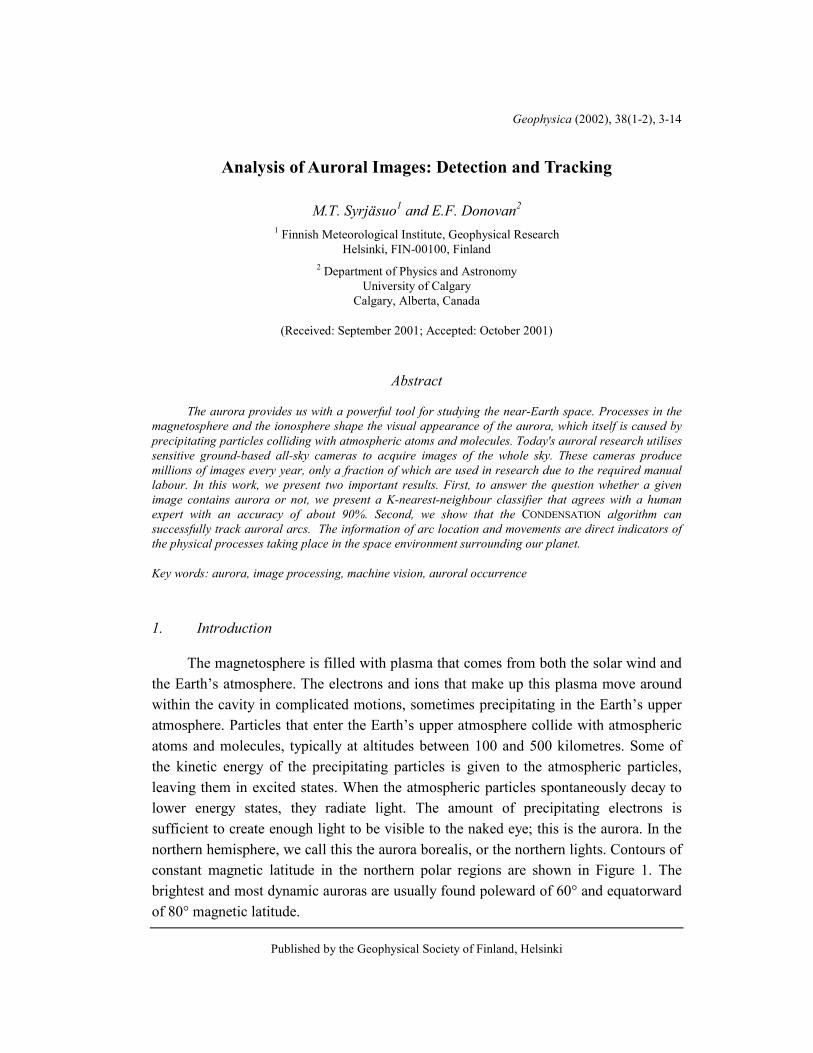
The magnetosphere is filled with plasma that comes from both the solar wind and the Earth’s atmosphere. The electrons and ions that make up this plasma move around within the cavity in complicated motions, sometimes precipitating in the Earth’s upper atmosphere. Particles that enter the Earth’s upper atmosphere collide with atmospheric atoms and molecules, typically at altitudes between 100 and 500 kilometres. Some of the kinetic energy of the precipitating particles is given to the atmospheric particles, leaving them in excited states. When the atmospheric particles spontaneously decay to lower energy states, they radiate light. The amount of precipitating electrons is sufficient to create enough light to be visible to the naked eye; this is the aurora. In the northern hemisphere, we call this the aurora borealis, or the northern lights. Contours of constant magnetic latitude in the northern polar regions are shown in Figure 1. The brightest and most dynamic auroras are usually found poleward of 60° and equatorward of 80° magnetic latitude.

Published by the Geophysical Society of Finland, Helsinki

M.T. Syrjäsuo and E.F. Donovan 4

Though always present, the intensity, location and structure of the aurora is virtually ever-changing. Early work in space physics led to the realisation that changes in the aurora are directly coupled to dynamics within the magnetosphere and the solar wind, and hence that the aurora provides us with a powerful tool for studying the plasma environment in near-Earth space.

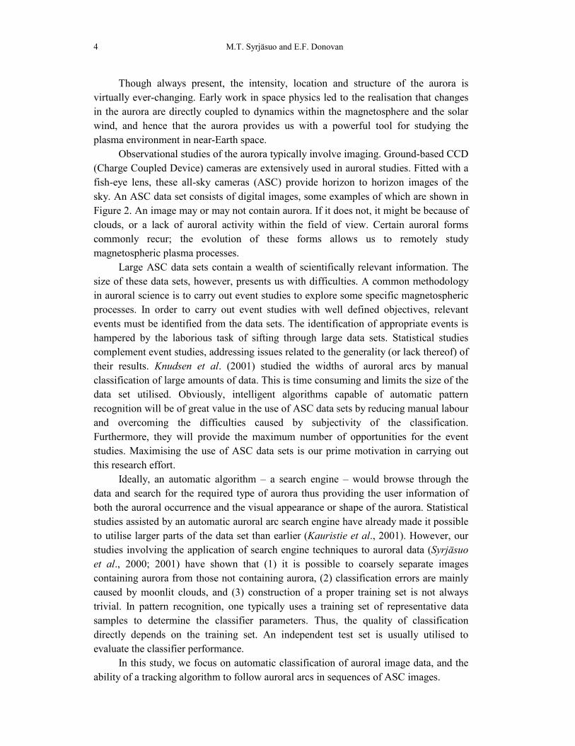
Observational studies of the aurora typically involve imaging. Ground-based CCD (Charge Coupled Device) cameras are extensively used in auroral studies. Fitted with a fish-eye lens, these all-sky cameras (ASC) provide horizon to horizon images of the sky. An ASC data set consists of digital images, some examples of which are shown in Figure 2. An image may or may not contain aurora. If it does not, it might be because of clouds, or a lack of auroral activity within the field of view. Certain auroral forms commonly recur; the evolution of these forms allows us to remotely study magnetospheric plasma processes.

Large ASC data sets contain a wealth of scientifically relevant information. The size of these data sets, however, presents us with difficulties. A common methodology in auroral science is to carry out event studies to explore some specific magnetospheric processes. In order to carry out event studies with well defined objectives, relevant events must be identified from the data sets. The identification of appropriate events is hampered by the laborious task of sifting through large data sets. Statistical studies complement event studies, addressing issues related to the generality (or lack thereof) of their results. Knudsen et al. (2001) studied the widths of auroral arcs by manual classification of large amounts of data. This is time consuming and limits the size of the data set utilised. Obviously, intelligent algorithms capable of automatic pattern recognition will be of great value in the use of ASC data sets by reducing manual labour and overcoming the difficulties caused by subjectivity of the classification. Furthermore, they will provide the maximum number of opportunities for the event studies. Maximising the use of ASC data sets is our prime motivation in carrying out this research effort.

Ideally, an automatic algorithm – a search engine – would browse through the data and search for the required type of aurora thus providing the user information of both the auroral occurrence and the visual appearance or shape of the aurora. Statistical studies assisted by an automatic auroral arc search engine have already made it possible to utilise larger parts of the data set than earlier (Kauristie et al., 2001). However, our studies involving the application of search engine techniques to auroral data (Syrjäsuo et al., 2000; 2001) have shown that (1) it is possible to coarsely separate images containing aurora from those not containing aurora, (2) classification errors are mainly caused by moonlit clouds, and (3) construction of a proper training set is not always trivial. In pattern recognition, one typically uses a training set of representative data samples to determine the classifier parameters. Thus, the quality of classification directly depends on the training set. An independent test set is usually utilised to evaluate the classifier performance.

In this study, we focus on automatic classification of auroral image data, and the ability of a tracking algorithm to follow auroral arcs in sequences of ASC images.

Analysis of Auroral Images: Detection and Tracking 5

Fig. 1. Map of the northern polar regions, showing contours of constant magnetic latitude. Bright auroral emissions occur most commonly at latitudes between 60° and 80° magnetic latitude. The 160° field of view (FOV) of the auroral imagers are shown; this FOV discards the lowest 10° degrees of elevation angle which provide the least accurate data. The imager arrays are described in section 2.

Fig. 2. Four examples of commonly occurring auroral forms. From left to right, these are: 1) auroral arc; 2) auroral band (ripples on an auroral arc); 3) an omega band-like distortion of diffuse aurora; 4) streamers intruding into the field of view from the north. North is towards the top of the figure.

2. Data

There are several ground-based observation programs that involve operation of ASCs and other instruments such as photometers, magnetometers, riometers and radars. These instrument arrays provide a comprehensive quantitative picture of the impact of magnetospheric dynamics on the Earth’s upper atmosphere and hence on the state and dynamics of the magnetosphere. Two such programs are MIRACLE (for Magnetometers, Ionospheric Radars, and All-sky Cameras Large Experiment) (Syrjäsuo et al., 1998) and CANOPUS (for Canadian Auroral Network for the OPEN Program Unified Study) (Rostoker et al., 1995). The fields of view of the one CANOPUS and eight MIRACLE ASCs are shown in Figure 1.

M.T. Syrjäsuo and E.F. Donovan 6

The data used in this study was obtained from the CANOPUS and MIRACLE ASC data sets. The ASCs are similar in both networks: a fish-eye lens captures the whole sky, narrow bandpass filters are used to choose a scientifically meaningful spectral line, and after intensification the image is recorded by a CCD camera (the CANOPUS and MIRACLE CCDs are 256 × 256 and 512 × 512 pixel devices, respectively). The resulting circular images are 8-bit grey-scale images. On average CANOPUS produces about 60000 images annually, whereas the eight MIRACLE cameras typically record over five million images every year. The CANOPUS and MIRACLE ASCs obtain images through 427.8 nm, 557.7 nm, and 630.0 nm filters. Due to CCD and intensifier performance issues and details of the auroral process, the 557.7 nm images in both data sets show the brightest, clearest and most dynamic structures. Almost all auroral all-sky cameras record this spectral line, which makes the presented classification technique applicable to other imagers, too. Consequently, we restrict our attention to the 557.7 nm data.

3. Classifying individual images

3.1 Construction of the training and test sets

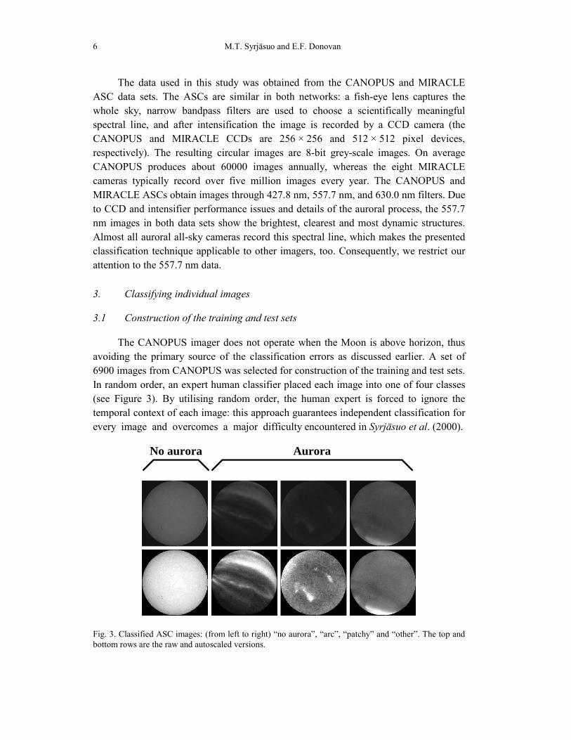
The CANOPUS imager does not operate when the Moon is above horizon, thus avoiding the primary source of the classification errors as discussed earlier. A set of 6900 images from CANOPUS was selected for construction of the training and test sets. In random order, an expert human classifier placed each image into one of four classes (see Figure 3). By utilising random order, the human expert is forced to ignore the temporal context of each image: this approach guarantees independent classification for every image and overcomes a major difficulty encountered in Syrjäsuo et al. (2000).

No aurora Aurora

Fig. 3. Classified ASC images: (from left to right) “no aurora”, “arc”, “patchy” and “other”. The top and bottom rows are the raw and autoscaled versions.

Analysis of Auroral Images: Detection and Tracking 7

One class was no aurora. The other three were distinct, though broad, classes of auroras. The training set consisted of 760 “no aurora” images and 760 “aurora” images. The latter class was constructed by merging all auroral classes into one superclass. The test set consisted of the remaining 5380 images, similarly divided into two classes.

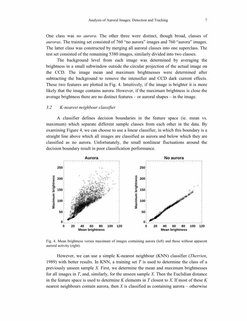
The background level from each image was determined by averaging the brightness in a small subwindow outside the circular projection of the actual image on the CCD. The image mean and maximum brightnesses were determined after subtracting the background to remove the intensifier and CCD dark current effects. These two features are plotted in Fig. 4. Intuitively, if the image is brighter it is more likely that the image contains aurora. However, if the maximum brightness is close the average brightness there are no distinct features – or auroral shapes – in the image.

3.2 K-nearest neighbour classifier

A classifier defines decision boundaries in the feature space (ie. mean vs. maximum) which separate different sample classes from each other in the data. By examining Figure 4, we can choose to use a linear classifier, in which this boundary is a straight line above which all images are classified as aurora and below which they are classified as no aurora. Unfortunately, the small nonlinear fluctuations around the decision boundary result in poor classification performance.

Aurora

0 20 40 60 80 100 120Mean brightness

0

50

100

150

200

250

Max

imu

m b

rig

htn

ess

No aurora

0 20 40 60 80 100 120Mean brightness

0

50

100

150

200

250

Max

imu

m b

rig

htn

ess

Fig. 4. Mean brightness versus maximum of images containing aurora (left) and those without apparent auroral activity (right).

However, we can use a simple K-nearest neighbour (KNN) classifier (Therrien, 1989) with better results. In KNN, a training set T is used to determine the class of a previously unseen sample X. First, we determine the mean and maximum brightnesses for all images in T, and, similarly, for the unseen sample X. Then the Euclidian distance in the feature space is used to determine K elements in T closest to X. If most of these K nearest neighbours contain aurora, then X is classified as containing aurora – otherwise

M.T. Syrjäsuo and E.F. Donovan 8

it is classified as no aurora. This classification scheme clearly defines nonlinear decision boundaries and thus improves the performance.

We found that, with K = 17, the classification of CANOPUS images is ~ 92% accurate, which is good enough for most statistical applications. The accuracy was determined by comparing the classification of the KNN classifier to that of the human expert. Furthermore, the feature distribution suggests that the number of datapoints used in the example set T can be considerably reduced for faster processing: only those examples that are close to the decision boundary are actually required.

3.3 Auroral occurrence in Kevo in 1997-98

Nevanlinna and Pulkkinen (2001) utilised an auroral occurrence index AO for studying the visibility of auroras in Finland. The AO index is based on determining the relationship between positive (ie. with aurora) and negative auroral (ie. no aurora) observations during clear nights. In percentage,

AO = 100A/(A + C), (1)

where A is the cumulative duration of auroral light during a given hour and, similarly, C is the total time with clear sky and no auroras visible for the same hour.

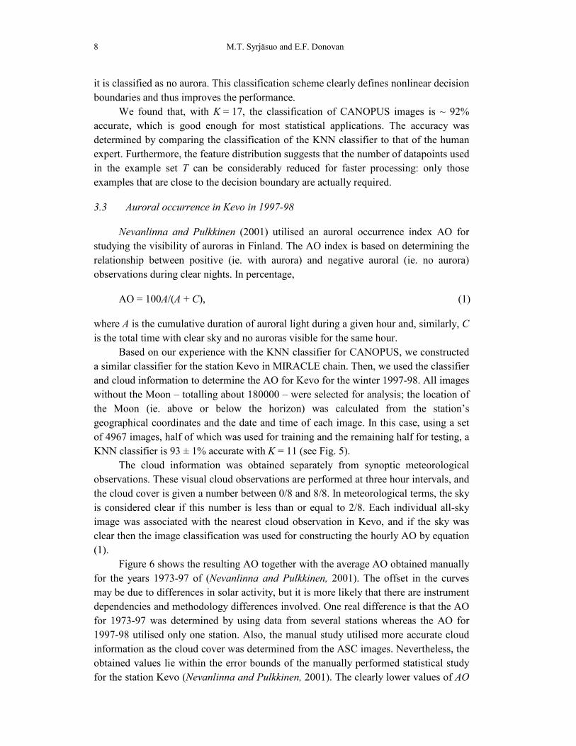
Based on our experience with the KNN classifier for CANOPUS, we constructed a similar classifier for the station Kevo in MIRACLE chain. Then, we used the classifier and cloud information to determine the AO for Kevo for the winter 1997-98. All images without the Moon – totalling about 180000 – were selected for analysis; the location of the Moon (ie. above or below the horizon) was calculated from the station’s geographical coordinates and the date and time of each image. In this case, using a set of 4967 images, half of which was used for training and the remaining half for testing, a KNN classifier is 93 ± 1% accurate with K = 11 (see Fig. 5).

The cloud information was obtained separately from synoptic meteorological observations. These visual cloud observations are performed at three hour intervals, and the cloud cover is given a number between 0/8 and 8/8. In meteorological terms, the sky is considered clear if this number is less than or equal to 2/8. Each individual all-sky image was associated with the nearest cloud observation in Kevo, and if the sky was clear then the image classification was used for constructing the hourly AO by equation (1).

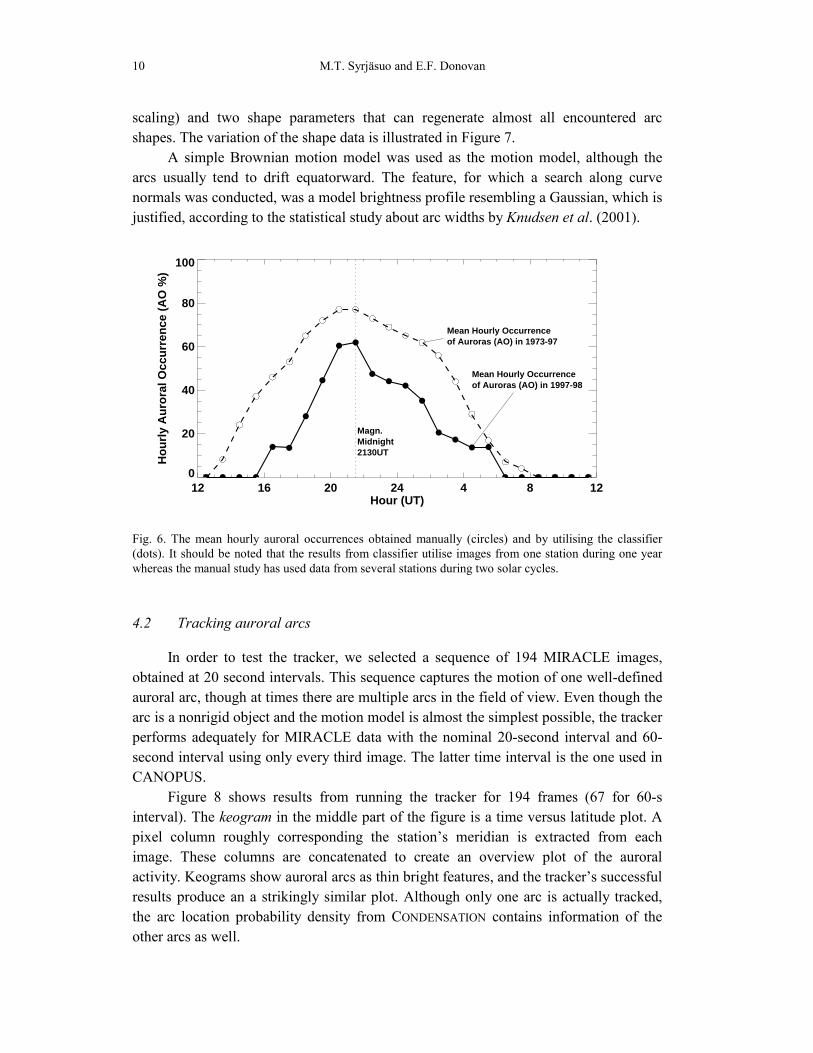
Figure 6 shows the resulting AO together with the average AO obtained manually for the years 1973-97 of (Nevanlinna and Pulkkinen, 2001). The offset in the curves may be due to differences in solar activity, but it is more likely that there are instrument dependencies and methodology differences involved. One real difference is that the AO for 1973-97 was determined by using data from several stations whereas the AO for 1997-98 utilised only one station. Also, the manual study utilised more accurate cloud information as the cloud cover was determined from the ASC images. Nevertheless, the obtained values lie within the error bounds of the manually performed statistical study for the station Kevo (Nevanlinna and Pulkkinen, 2001). The clearly lower values of AO

Analysis of Auroral Images: Detection and Tracking 9

between 08-15 UT are due to unused data: if the Sun is not far below the horizon, the refracted sunlight imitates the appearance of aurora and causes misclassification. Thus, the images from late morning and early morning were not utilised. One should also note that at the latitude of the station Kevo, daylight prevents auroral observations between 08-12 UT.

0 5 10 15 20 25 30 35K in KNN

6

8

10

12

14

16

18

20

To

tal e

rro

r (%

)

Fig. 5. The classification error as a function of K in KNN classification – upper and lower bounds are shown. The bounds are estimated by classifying all images (lower bound) and using a “leave-one-out”-technique (upper bound) (Therrien, 1989).

4. Tracking aurora

4.1 Motivation and tracker details

Once the images containing aurora have been found, tracking of aurora makes it possible to collect information about auroral shapes automatically. It also allows the estimation of process parameters for the visual appearance of aurora by providing accurate location information together with their temporal changes. This can be utilised in constructing mathematical models for both auroral shapes and their behaviour.

We used the CONDENSATION tracker introduced by Isard and Blake (1998). This stochastic tracker utilises random sampling technique together with a shape and motion model for tracking objects in noisy and cluttered scene. We used B-splines (Bartels et al., 1987) to represent the arc shape. A visually pleasing arc required six spline control points (x- and y-coordinates for each point) resulting in a 12-dimensional parameter space.

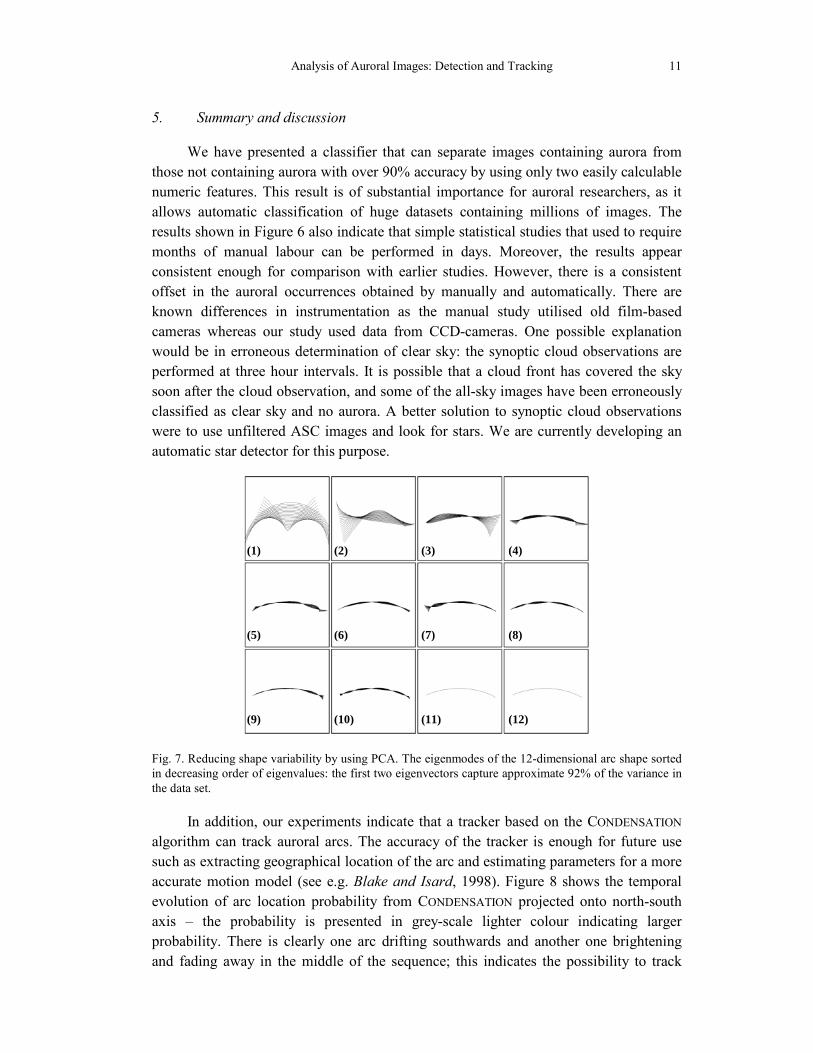
To reduce the dimensionality, we utilised Principal Component Analysis (PCA) on a set of 746 manually fine-tuned and confirmed arc shapes from MIRACLE data (Isard and Blake, 1998). This resulted in a 6-dimensional shape space consisting of Euclidean transformations (ie. four parameters for translation, rotation and isotropic

M.T. Syrjäsuo and E.F. Donovan 10

scaling) and two shape parameters that can regenerate almost all encountered arc shapes. The variation of the shape data is illustrated in Figure 7.

A simple Brownian motion model was used as the motion model, although the arcs usually tend to drift equatorward. The feature, for which a search along curve normals was conducted, was a model brightness profile resembling a Gaussian, which is justified, according to the statistical study about arc widths by Knudsen et al. (2001).

12 16 20 24 4 8 12Hour (UT)

0

20

40

60

80

100

Ho

url

y A

uro

ral O

ccu

rren

ce (

AO

%)

Magn.Midnight2130UT

Mean Hourly Occurrenceof Auroras (AO) in 1997-98

Mean Hourly Occurrenceof Auroras (AO) in 1973-97

Fig. 6. The mean hourly auroral occurrences obtained manually (circles) and by utilising the classifier (dots). It should be noted that the results from classifier utilise images from one station during one year whereas the manual study has used data from several stations during two solar cycles.

4.2 Tracking auroral arcs

In order to test the tracker, we selected a sequence of 194 MIRACLE images, obtained at 20 second intervals. This sequence captures the motion of one well-defined auroral arc, though at times there are multiple arcs in the field of view. Even though the arc is a nonrigid object and the motion model is almost the simplest possible, the tracker performs adequately for MIRACLE data with the nominal 20-second interval and 60-second interval using only every third image. The latter time interval is the one used in CANOPUS.

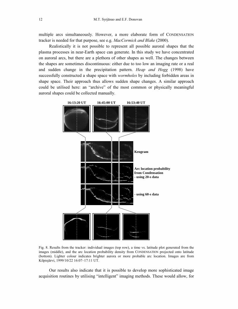
Figure 8 shows results from running the tracker for 194 frames (67 for 60-s interval). The keogram in the middle part of the figure is a time versus latitude plot. A pixel column roughly corresponding the station’s meridian is extracted from each image. These columns are concatenated to create an overview plot of the auroral activity. Keograms show auroral arcs as thin bright features, and the tracker’s successful results produce an a strikingly similar plot. Although only one arc is actually tracked, the arc location probability density from CONDENSATION contains information of the other arcs as well.

Analysis of Auroral Images: Detection and Tracking 11

5. Summary and discussion

We have presented a classifier that can separate images containing aurora from those not containing aurora with over 90% accuracy by using only two easily calculable numeric features. This result is of substantial importance for auroral researchers, as it allows automatic classification of huge datasets containing millions of images. The results shown in Figure 6 also indicate that simple statistical studies that used to require months of manual labour can be performed in days. Moreover, the results appear consistent enough for comparison with earlier studies. However, there is a consistent offset in the auroral occurrences obtained by manually and automatically. There are known differences in instrumentation as the manual study utilised old film-based cameras whereas our study used data from CCD-cameras. One possible explanation would be in erroneous determination of clear sky: the synoptic cloud observations are performed at three hour intervals. It is possible that a cloud front has covered the sky soon after the cloud observation, and some of the all-sky images have been erroneously classified as clear sky and no aurora. A better solution to synoptic cloud observations were to use unfiltered ASC images and look for stars. We are currently developing an automatic star detector for this purpose.

(1) (2) (3) (4)

(5) (6) (7) (8)

(9) (10) (11) (12)

Fig. 7. Reducing shape variability by using PCA. The eigenmodes of the 12-dimensional arc shape sorted in decreasing order of eigenvalues: the first two eigenvectors capture approximate 92% of the variance in the data set.

In addition, our experiments indicate that a tracker based on the CONDENSATION algorithm can track auroral arcs. The accuracy of the tracker is enough for future use such as extracting geographical location of the arc and estimating parameters for a more accurate motion model (see e.g. Blake and Isard, 1998). Figure 8 shows the temporal evolution of arc location probability from CONDENSATION projected onto north-south axis – the probability is presented in grey-scale lighter colour indicating larger probability. There is clearly one arc drifting southwards and another one brightening and fading away in the middle of the sequence; this indicates the possibility to track

M.T. Syrjäsuo and E.F. Donovan 12

multiple arcs simultaneously. However, a more elaborate form of CONDENSATION tracker is needed for that purpose, see e.g. MacCormick and Blake (2000).

Realistically it is not possible to represent all possible auroral shapes that the plasma processes in near-Earth space can generate. In this study we have concentrated on auroral arcs, but there are a plethora of other shapes as well. The changes between the shapes are sometimes discontinuous: either due to too low an imaging rate or a real and sudden change in the precipitation pattern. Heap and Hogg (1998) have successfully constructed a shape space with wormholes by including forbidden areas in shape space. Their approach thus allows sudden shape changes. A similar approach could be utilised here: an “archive” of the most common or physically meaningful auroral shapes could be collected manually.

16:13:20 UT 16:45:00 UT 16:53:40 UT

Keogram

Arc location probabilityfrom Condensation- using 20-s data

- using 60-s data

Fig. 8. Results from the tracker: individual images (top row), a time vs. latitude plot generated from the images (middle), and the arc location probability density from CONDENSATION projected onto latitude (bottom). Lighter colour indicates brighter aurora or more probable arc location. Images are from Kilpisjärvi, 1999/10/22 16:07–17:11 UT.

Our results also indicate that it is possible to develop more sophisticated image acquisition routines by utilising “intelligent” imaging methods. These would allow, for

Analysis of Auroral Images: Detection and Tracking 13

example, increased temporal resolution whenever the characteristic timescale of auroral activity requires it.

While the KNN classifier can be used for practically all images without the Moon, the tracker is more suited for case studies in which the time period is already known. However, the tracker can assist in finding drift velocities and accurate geographical locations required for, say, mapping ionospheric measurements to magnetosphere.

Acknowledgements

MIRACLE and CANOPUS are operated under the leadership of the Finnish Meteorological Institute and the Canadian Space Agency, respectively. K. Kauristie and L.L. Cogger are the Principal Investigators of the MIRACLE and CANOPUS ASC projects, respectively. We acknowledge the financial support of the Natural Sciences and Engineering Research Council (Canada), and the Vilho, Yrjö and Kalle Väisälä Foundation (Finland).

References

Bartels, B., J. Beatty and B. Barsky, 1987. An introduction to splines for use in computer graphics and geometrical modeling. Morgan Kaufmann.

Blake A. and M. Isard, 1998. Active contours. Springer. Heap, T. and D. Hogg, 1998. Wormholes in shape space: tracking through

discontinuous changes in shape. In Proc. of the International Conference on Computer vision, pp. 344-349.

Isard, M. and A. Blake, 1998. CONDENSATION – conditional density propagation for visual tracking. Int. J. Computer Vision, 29(1), 5-28.

Kauristie, K., M. Syrjäsuo, O. Amm, A. Viljanen, T. Pulkkinen and H. Opgenoorth, 2001. Statistical study of evening sector arcs and electrojets. Advances in Space Research, Vol. 28, No. 11, 1605-1610.

Knudsen, D.J., E.F. Donovan, L.L. Cogger, B. Jackel and W.D. Shaw, 2001. Width and structure of mesoscale optical auroral arcs. Geophysical Research Letters, 28, 705-708.

MacCormick, J. and A. Blake, 2000. Probabilistic exclusion and partitioned sampling for multiple objects. Int. J. Computer Vision, 39(1), 57-71.

Nevanlinna, H. and T. Pulkkinen, 2001. Auroral observations in Finland: results from all-sky cameras, 1973-1997. J. Geophys. Res., 106, 8109-8118.

Rostoker, G., J.C. Samson, F. Creutzberg, T.J. Hughes, D.R. McDiarmid, A. McNamara, A.G. Vallance-Jones, D.D. Wallis and L.L. Cogger, 1995. CANOPUS – a ground-based instrument array for remote sensing of the high-latitude ionosphere during the ISTP/GGS Program. Space Science Reviews, 71, 743-760.

Syrjäsuo, M.T., K. Kauristie and T.I. Pulkkinen, 2000. Searching for aurora. In Proc. of the IASTED Int. Conf. on Signal and Image Processing, SIP-2000, pp. 381-386.

M.T. Syrjäsuo and E.F. Donovan 14

Syrjäsuo, M.T., K. Kauristie and T.I. Pulkkinen, 2001. A search engine for auroral forms. Advances in Space Research, Vol. 28, No. 11, pp. 1611-1616.

Syrjäsuo M.T, T.I. Pulkkinen, R.J. Pellinen, P. Janhunen, K. Kauristie, A. Viljanen, H.J. Opgenoorth, P. Karlsson, S. Wallman, P. Eglitis, O. Amm, E. Nielsen and C. Thomas, 1998. Observations of substorm electrodynamics using the MIRACLE network, In: S. Kokubun and Y. Kamide (eds), Proceedings of the International Conference on Substorms-4: Astrophysics and Space Science Library, Vol. 238, Terra Scientific Publishing Company. Kluwer Academic Publishers, pp. 111-114.

Therrien, C.W., 1989. Decision, estimation and classification. John Wiley & Sons.