THE ARGO AUTONOMOUS VEHICLE’S VISION AND ... Journal of Intelligent Control and Systems Vol. 3, No. 4 (1999) 409{441 c World Scienti c Publishing Company THE ARGO AUTONOMOUS VEHICLE’S

International Journal of Intelligent Control and SystemsVol. 3, No. 4 (1999) 409–441c©World Scientific Publishing Company

THE ARGO AUTONOMOUS VEHICLE’SVISION AND CONTROL SYSTEMS∗

ALBERTO BROGGI

Dip. di Informatica e Sistemistica, Universita di Pavia, Via Ferrata 1

Pavia, I-27100 Pavia, Italy

MASSIMO BERTOZZI, ALESSANDRA FASCIOLI

CORRADO GUARINO LO BIANCO, AURELIO PIAZZI

Dip. di Ingegneria dell’Informazione, Universita di Parma, Parco Area delle Scienze 181AParma, I-43100 Parma, Italy

Received (November 1999)Revised (May 2000)

This paper presents the current status of the ARGO Project, whose main target is the de-velopment of an active safety system and an automatic pilot for a standard road vehicle.

First the ARGO project is briefly described along with its main objectives, then the pro-

totype vehicle and its functionalities are presented. The perception of the environment isperformed through the processing of images acquired from the vehicle; details about the

detection of lane markings, generic obstacles and leading vehicles are given. The paperdescribes the current implementation of the control system, based on a gain scheduled

controller, which allows the vehicle to follow the road and/or other vehicles, while future

control strategies (flatness approach) are presented with simulations results. The paperends with a description of the MilleMiglia in Automatico tour, a journey through Italy

performed in automatic driving, together with some concluding remarks.

Keywords: Vision-based autonomous vehicle, Image processing, Obstacle detection, Lane

detection, Vehicle detection, Visual servoing, Automatic steering, Flatness approach,Trajectory planning.

1. Introduction

Automatic Vehicle Driving is a generic term used to address a technique aimed atautomating –entirely or in part– one or more driving tasks. The automation ofthese tasks carries a large number of benefits, such as: a higher exploitation of theroad network, lower fuel and energy consumption, and –of course– improved safetyconditions compared to the current scenario.

The tasks that automatically driven vehicles are able to perform include thepossibility to follow the road and keep within the right lane, maintaining a safe∗This research has been partially supported by the Italian MURST and CNR under the frame ofProgetto Madess 2 and under the contract n. 99.00619.CT12.

409

410 A. Broggi et al.

distance between vehicles, regulating the vehicle’s speed according to traffic condi-tions and road characteristics, moving across lanes in order to overtake vehicles andavoid obstacles, helping to find the correct and shortest route to a destination, andthe movement and parking within urban environments.

Two main cooperative solutions are possible to achieve automatic driving func-tionalities: they require to act on infrastructures or vehicles. Both scenarios havetheir own pros and cons, depending on the specific application1; the research doc-umented in this paper is focused exclusively on vehicles.

The following section presents the ARGO project and the prototype vehicledeveloped within this framework. The vehicle has visual and control capabilities:section 3 describes how the ARGO prototype vehicle can perceive the surroundingenvironment and the basics of lane and vehicle detection functionalities, while sec-tion 4 describes the current control subsystem and a new method based on a flatnessapproach. Section 5 gives an overview of the extensive test, called MilleMiglia inAutomatico, that took place in 1998 when the vehicle drove itself for more than2000 km in automatic mode on Italian highways, and section 6 presents some con-cluding remarks and possible future research directions.

2. The ARGO Project

The main target of the ARGO Project1 is the development of an active safety systemwhich can also act as an automatic pilot for a standard road vehicle.

In order to achieve an autonomous driving system which fits into the existingroad network with no need for specific infrastructures, the capability of perceivingthe environment is essential for the intelligent vehicle. Although very efficient insome fields of application, active sensors –besides polluting the environment– featuresome specific problems in automotive applications due to inter-vehicle interferenceamongst the same type of sensors, and due to the wide variation in reflection ratioscaused by many different reasons, such as obstacles’ shape or material. Moreover,the maximum signal level must comply with safety rules and must be lower than asafety threshold. For this reason in the implementation of the ARGO vehicle onlythe use of passive sensors, such as cameras, has been considered.

A second design choice was to keep the system costs low. These costs includeboth production costs (which must be minimized to allow a widespread use of thesedevices) and operative costs, which must not exceed a certain threshold in ordernot to interfere with the vehicle performance. Therefore low cost devices have beenpreferred, both for the image acquisition and the processing: the prototype installedon ARGO is based on cheap cameras and a commercial PC.

2.1. The ARGO Vehicle Prototype

ARGO, shown in figure 1, is an experimental autonomous vehicle equipped withvision systems and an automatic steering capability.

It is able to determine its position with respect to the lane, to compute the road

The ARGO Autonomous Vehicle’s Vision and Control Systems 411

Fig. 1. The ARGO prototype vehicle.

geometry, to detect generic obstacles on the path, and to localize a leading vehicle.The images acquired by a stereo rig placed inside the windscreen are analyzed inreal-time by a computing system located into the boot. The results of the processingare used to drive an actuator mounted onto the steering wheel and other drivingassistance devices.

The system was initially conceived as a safety enhancement unit: in particular itis able to supervise the driver behavior and issue both optic and acoustic warningsor even take control of the vehicle when dangerous situations are detected. Furtherdevelopments have extended the system functionalities to automatic driving.

2.1.1. The Data Acquisition System

Only passive sensors (two cameras and a speedometer) are used on ARGO to sensethe surrounding environment. In addition, a button-based control panel has beeninstalled enabling the driver to modify a few driving parameters, select the systemfunctionality, issue commands, and interact with the system.

The stereoscopic vision system installed on ARGO consists of two low cost syn-chronized cameras able to acquire pairs of grey level images simultaneously. Thecameras lie inside the vehicle at the top corners of the windscreen, so that thelongitudinal distance between the two cameras is maximum.

The vehicle is also equipped with a speedometer to detect its velocity. A Halleffect-based device has been chosen due to its simplicity and its reliability and hasbeen interfaced to the computing system via a digital I/O board with event countingcapabilities. The resolution of the measuring system is about 9 cm/s.


2.1.2. The Processing System

The architectural solution currently installed on the ARGO vehicle is based on astandard 450 MHz Pentium II processor. Thanks to recent advances in computertechnologies, commercial systems offer nowadays sufficient computational power forthis application. All the processing needed for the driving task (image featureextraction and vehicle trajectory control) is performed in real-time: 50 single fieldimages are processed every second.

2.1.3. The Output System

Several output devices have been installed on ARGO (see figure 2).Acoustical (stereo loudspeakers) and optical (led-based control panel) devices

are used to issue warnings to the driver in case dangerous conditions are detected,while a color monitor is mainly used as a debugging tool.

A single mechanical device has been integrated on ARGO to provide autonomoussteering capabilities. It is composed of an electric stepping motor coupled to thesteering column by means of a belt. During automatic driving the output providedby the vision system is used to turn the steering wheel so to maintain the vehicleinside the lane or to follow the leading vehicle.

2.2. Automatic Driving Functionalities

Thanks to the control panel the driver can select the level of system intervention.The following three driving modes are integrated.Manual Driving: the system simply monitors and logs the driver’s activity.Supervised Driving: in case of dangerous situations the system warns the driverwith acoustic and optical signals.Automatic Driving: the system fully controls of the vehicle’s trajectory.

In the automatic driving operative mode two different functionalities can beselected: Road Following or Platooning.

The Road Following task, namely the automatic movement of the vehicle alongthe lane, is based on Lane Detection which includes the localization of the road, thedetermination of the relative position between vehicle and road, and the analysis ofthe vehicle’s heading direction.

Conversely, the Platooning functionality, namely the automatic following of thepreceding vehicle requires the localization and tracking of the target vehicle (VehicleDetection), which relies on the recognition of specific vehicle’s characteristics.

3. Visual Perception of the Environment

In this section the vision algorithms implemented on the ARGO vehicle are de-scribed. Initially the extraction of the road geometry from monocular images ispresented. Then, the algorithm for the recognition and localization of the preced-ing vehicle is discussed.


3.1. Lane Detection

The Lane Detection functionality is based on the removal of the perspective effect

Electric engine

TV monitor

Right cameraLeft camera

Control panel

Emergency buttons

Emergency pedal

Fig. 2. Internal view of the ARGO vehicle.


(a) (b)

(c) (d) (e) (f)

Fig. 3. The sequence of images produced by the low-level Lane Detection phase: (a) original;

(b) remapped; (c) filtered; (d) binarized; (e) chains; (f ) polylines.

obtained through the Inverse Perspective Mapping (IPM).1 The IPM allows toremove the perspective effect from incoming images remapping each pixel toward adifferent position. It exploits a knowledge about the acquisition parameters (cameraorientation, position, optics,. . . ) and the assumption of a flat road in front of thevehicle. The result is a new 2-dimensional array of pixels (the remapped image) thatrepresents a bird’s eye view of the road region in front of the vehicle. Figures 3.aand 3.b show an image acquired by the ARGO vision system and the correspondingremapped image respectively.

The following steps are divided in low level and high level processing.

3.1.1. Low Level Processing for Lane Detection

In the remapped image a road marking resembles a semi-vertical line of constantwidth brighter than the dark road background. Therefore, road marking’s pixelsfeature a higher brightness value than their horizontal left and right neighbors ata given distance. Consequently, the first phase of road markings detection is basedon the determination of horizontal black-white-black transitions, while the followingprocess is aimed at extracting information and reconstructing road geometry.

Feature ExtractionThe brightness value of a generic pixel belonging to the remapped image is comparedto the two horizontal left and right neighbors at a given distance. A new image,


whose values encode the presence of a road marking, is computed assigning:

1. zero to the pixels whose one or both of the two neighbors have a higherbrightness value, or

2. the absolute difference between the pixel’s brightness and their neighbors’ onesto the pixels whose brightness is higher than the ones of the two neighbors.

The resulting filtered image is shown in figure 3.c.Due to different light conditions (e.g. in presence of shadows), pixels represent-

ing road markings may have different brightness, yet maintaining their superiorityrelationship with their horizontal neighbors. Therefore, since a simple threshold sel-dom gives a satisfactory binarization, the image is enhanced exploiting its verticalcorrelation. The result is presented in figure 3.d.

Road Geometry ReconstructionThe binary image is scanned row by row in order to build chains of 8-connectednon-zero pixels (see figure 3.e).

Subsequently, each chain is approximated with a polyline composed by one or fewsegments, by means of an iterative process. Initially, a single segment that joins thetwo extrema of the chain is considered. The horizontal distance between segment’smid point and the chain is used to determine the quality of the approximation. Incase it is larger than a threshold, two segments sharing an extremum are consideredfor the approximation of the chain. Their common extremum is the intersectionbetween the chain and the horizontal line that passes through the segment’s midpoint. The process is iterated until a satisfactory approximation has been reached.At the end of the processing all chains are approximated by polylines (see figure 3.f).

3.1.2. High Level Processing for Lane Detection

After the first low level stage, in which the main features are localized, and afterthe second stage, in which the main features are extracted, the new data structure(a list of polylines) is now processed in order to semantically group homologousfeatures and to produce a high level description of the scene.

This process in divided into: filtering of noisy features and selection of thefeature that most likely belong to the line marking; joining of different segments inorder to fill gaps caused by occlusions, dashed lines, or even worn lines; selection ofthe best representative and reconstruction of the information that may have beenlost, on the basis of continuity constraints; then the result is kept for reference inthe next frames and displayed onto the original image.

Feature filtering and selectionEach polyline is compared against the result of the previous frame, since continuityconstraints provide a strong and robust selection procedure. The distance betweenthe previous result and each extremum of the considered polyline is computed: if all


� � � ��

� � � ��

� � � � ��

� � � � ��

� � � � � ��

� � � � � ��

� � � � ��

� � � � ��

� � � � ��

� � � � ��

� � ��

� � � � ��

� � � � ��

� � � � ��

� � � � ��

� � � ��

� � � ��

� � � ��

� � � ��

� � � ��

� � � ��

� � � ��

� � � ��

� � ��

A

D

B

EC

F

Polyline

Linear approximation

Parabolicapproximation

(a) (b) (c)Fig. 4. High level processing for Lane Detection, first steps: (a) selection of polylines almostmatching the previous left result, (b) joining of similar polylines, (c) continuation of short polylines.

the polyline extrema lay within a stripe centered onto the previous result then thepolyline is marked as useful for the following process. This stripe is shaped so thatit is small at the bottom of the image (namely close to the vehicle, therefore shortmovements are allowed) and larger at the top of the image (far from the vehicle,where also curves that appear quickly must be tracked). This process is repeatedfor both left and right lane markings.

Figure 4.a shows the previous result with a heavy solid line and the search spacewith a gridded pattern; it refers to the left lane marking.

Polylines joiningOnce the polylines have been selected, all the possibilities are checked for theirjoining. In order to be joined, two polylines must have similar direction; must benot too far away; their projection on the vertical axis must not overlap; the higherpolyline in the image must have its starting point within an elliptical portion ofthe image; in case the gap is large also the direction of the connecting segment ischecked for uniform behavior. Figure 4.b shows that polyline A cannot be connectedto: B due to high difference of orientation; C due to high distance (does not laywithin the ellipse); D due to the overlapping of their vertical projections; E sincetheir connecting segment would have a strongly mismatching orientation. It canonly be connected to F.

Selection of the best representativeAll the new polylines, formed by concatenations of the original ones, are then evalu-ated. Starting from a maximum score, each of the following rules provides a penalty.First each polyline is segmented; in case the polyline does not cover the whole im-age, a penalty is given. Then, the polyline length is computed and a proportionalpenalty is given to short ones, as well as to polylines with extremely varying angu-lar coefficients. Finally, the polyline with the highest score is selected as the bestrepresentative of the line marking.


Reconstruction of lost informationThe polyline that has been selected at the previous step may not be long enough tocover the whole image; therefore a further step is necessary to extend the polyline.In order to take into account road curves, a parabolic model has been selected tobe used in the prolongation of the polyline in the area far from the vehicle. In thenearby area, a linear approximation suffices. Figure 4.c shows the parabolic andlinear prolongation.

Model fittingThe two reconstructed polylines (one representing the left and one the right lanemarkings) are now matched against a model that encodes some more knowledgeabout the absolute and relative positions of both lane markings on a standard road.A model of a pair of parallel lines at a given distance (the lane width) and in aspecific position is initialized at the beginning of the process; a specific learningphase allows to adapt the model to errors in camera calibration (lines may benon perfectly parallel). Furthermore, this model can be slowly changed during theprocessing to adapt to new road conditions (lane width and lane position), thanksto a learning process running in the background.

The model is kept for reference: the two resulting polylines are fitted to thismodel and the final result is obtained as follows. First the two polylines are checkedfor non-parallel behavior; a small deviation is allowed since it may derive fromvehicle movements or deviations from the flat road assumption, that cause thecalibration to be temporarily incorrect (diverging of converging lane markings).

(high quality)Left polyline

(low quality)Right Polyline

Models

0.5

1

0

Weigth

Measured distance

Model distance

Final position

A B

Wr (weight right polyline)

Wl (weigth left polyline)

Quality = (Qright-Qleft)

A = (Model distance - Measured distance - K) * WrB = (Model distance - Measured distance - K) * Wl

H

h

Bd

Td

K = (Td - Bd) * h / H

Fig. 5. Generation of the final result.


Fig. 6. Filtered polylines, joined polylines, and model fitting for the left (upper row) and right

(bottom row) lane markings.

Then the quality of the two polylines, as computed in the previous steps, is matched:the final result will be attracted toward the polyline with the highest quality witha higher strength. In this way, polylines with equal or similar quality will equallycontribute to the final result; on the other hand, in case one polyline has beenheavily reconstructed, or is far from the original model, or is even missing, theother polyline will be used to generate the final result. The weights for the left andright polylines are computed as shown in figure 5. Then, each horizontal line of thetwo polylines is used to compute the final results, as shown in figure 5.

Finally figure 6 presents the resulting images referring to the example presentedin figure 3. It shows the results of the selection, the joining, and the matching phasephases for the left (upper row) and for the right (bottom row) lane markings.

Figure 7 presents the final result of the process.

(a) (b)Fig. 7. The result of lane detection: (a) the acquired image, (b) the result of lane detection shown

onto a saturated copy of the original image; black markers represent effective lane markings, whilewhite markings represent interpolations between them.


Fig. 8. Lane Detection: the result is shown with black markings superimposed onto a brighter

version of the original image.

3.1.3. Results of Lane Detection

Figure 8 presents a few results of lane detection in different conditions ranging fromideal situations to road works, patches of non-painted roads, the entry and exitfrom a tunnel. Both highway and extraurban scenes are provided for comparison;the systems proves to be robust with respect to different illumination situations,missing road signs, and overtaking vehicles which occlude the visibility of the leftlane marking. In case two lines are present, the system selects the continuous one.

Concerning the quantitative performance, the algorithm requires an overall av-erage time of 4 ms for the processing of a frame.

3.2. Vehicle Detection

The platooning functionality is based on the detection of the distance, speed, and


heading of the preceding vehicle, which is localized and tracked using a single monoc-ular image sequence.

The vehicle detection algorithm is based on the following considerations: a ve-hicle is generally symmetric, characterized by a rectangular bounding box whichsatisfies specific aspect ratio constraints, and placed in a particular region of theimage. These features are used to identify vehicles in the image in the followingway: first an area of interest is identified on the basis of road position and perspec-tive constraints. This area is searched for possible vertical symmetries; not onlygray level symmetries are considered, but vertical and horizontal edges symmetriesas well, in order to increase the detection robustness. Once the symmetry positionand width has been detected, a new search begins, which is aimed at the detectionof the two bottom corners of a rectangular bounding box. Finally, the top horizontallimit of the vehicle is searched for, and the preceding vehicle localized.

The tracking phase is performed through the maximization of the correlationbetween the portion of the image contained into the bounding box of the previousframe (partially stretched and reduced to take into account small size variationsdue to the increment or reduction of the relative distance) and the new frame.

Symmetry detectionIn order to search for symmetrical features, the analysis of gray level images isnot sufficient. Figure 9 shows that strong reflections cause irregularities in vehiclesymmetry, while uniform areas and background patterns present highly correlatedsymmetries. In order to cope with these problems, also symmetries in other domainsare computed.

Fig. 9. Typical road scenes: in the leftmost image a strong sun reflection reduces the vehicle

gray level symmetry; in the center image a uniform area can be regarded as a highly symmetricalregion; the rightmost image shows background symmetrical patterns.

To get rid of reflections and uniform areas, vertical and horizontal edges areextracted and thresholded, and symmetries are computed into these domains aswell. Figure 10 shows that although a strong reflection is present on the left sideof the vehicle, edges are anyway visible and can be used to extract symmetries;moreover, in uniform areas no edges are extracted and therefore no symmetries aredetected. Figure 11 shows two examples in which gray level symmetries alone can besuccessful for vehicle detection, while figure 12 shows the result of edge symmetry.


Fig. 10. Edges enforce the detection of real symmetries: strong reflections have lower effects while

uniform areas are discarded since they do not present edges.

Fig. 11. Grey level symmetries: the rightmost image for each case shows a symmetry map encoding

high symmetries with bright points.

Fig. 12. Edge symmetries: the symmetries are computed on the binary images obtained after

thresholding the gradient image.

For each image, the search area is shown in dark gray and the resulting verticalaxis is superimposed. For each image its symmetry map is also depicted both in itsoriginal size and –on the right– zoomed for better viewing. Bright points encodethe presence of high symmetries. The 2D symmetry maps are computed by varyingthe axis’ horizontal position within the grey area (shown in the original image) andthe symmetry horizontal size. The lower triangular shape is due to the limitationin scanning large horizontal windows for peripheral vertical axes.


Fig. 13. Computing the resulting symmetry: (a) grey-level symmetry; (b) edge symmetry; (c) hor-

izontal edges symmetry; (d) vertical edges symmetry; (e) total symmetry. For each row theresulting symmetry axis is superimposed onto the leftmost original image.

Similarly, the analysis of symmetries of horizontal and vertical edges producesother symmetry maps, which –with specific coefficients detected experimentally–can be combined with the previous ones to form a single symmetry map. Figure 13shows all symmetry maps and the final one, that allows to detect the vehicle.

Bounding box detectionAfter the localization of the symmetry, the symmetrical region is checked for thepresence of two corners representing the bottom of the bounding box around thevehicle. Perspective constraints as well as size constraints are used as search criteria.


Figure 14 presents the results of the lower corners detection.

Fig. 14. Detection of the lower part of the bounding box: (a) original image with symmetry axis;(b) edges; (c) localization of the two lower corners.

This process is followed by the detection of the top part of the bounding box,which is looked for in a specific region whose location is again determined by per-spective and size constraints.

BacktrackingSometimes it may happen that in correspondence to the symmetry maximum nocorrect bounding boxes exist. Therefore, a backtracking approach is used: thesymmetry map is again scanned for the next local maximum and a new search for abounding box is performed. Figure 15 shows a situation in which the first symmetrymaximum, generated by a building, does not lead to a correct bounding box; onthe other hand, the second maximum leads to the correct detection of the vehicle.

Fig. 15. A case in which the total background symmetry is higher than the vehicle symmetry.Original image; first symmetry map; second symmetry map after the backtracking process has

removed the peak near the maximum; final bounding box detection.


3.2.1. Results of Vehicle Detection

Figure 16 shows some qualitative results of vehicle detection in different situations:the preceding vehicle is correctly detected at different distances, even when severalother vehicles are present on the road.

The quantitative performance has also been assessed: the algorithm runs in23 ms when no vehicle has been detected in the previous frame and therefore a newsearch is started. However, the time required for the processing decreases to 9 mswhen the target vehicle is being tracked.

Fig. 16. Vehicle Detection: the images show the search area and the detected vehicle with black

markings superimposed onto a brighter version of the original image.

4. Vehicle Control

In recent years, the problem of automatic steering of an autonomous vehicle hasgained considerable attention from both the theoretical2,3 and experimental side.4,5

Roughly speaking this problem is centered on finding a satisfactory law forthe command of the steering wheel. Many works have been reported in the litera-ture6,7,8,9,10,11,12,13,14 and various steering control designs were proposed for systemsin which the sensing is performed with nonvisual devices (for example, guiding wire,microwave radars, etc.).

On the other hand, a visual servoing paradigm was proposed by Epiau et al.15 byconsidering a simple omnidirectional mobile robot. Neural networks were adoptedand subsequently developed in the RALPH project.16,17 A comparative survey onvarious vision-based control strategies for autonomous vehicles can be found in thepaper of Taylor et al.5

Subsection 4.1 presents the gain scheduled proportional controller currently im-plemented on the ARGO vehicle. By using a feedback supervisor this control lawcan be adopted to perform both path following and platooning. A simple propor-tional control law was previously examined by Ozguner et al.18 for the path followingfunctionality solely. Subsection 4.2 exposes a differential flatness approach that will


��

��

� �� !�"�# ��$&%'�(��*)

+-,/.10

2*3�4�3�5�67�8 9!8:<; 5>=

?

Fig. 17. Control scheme with the gain scheduled proportional controller.

d

�

��

�

Fig. 18. Offset from the desired path, estimated by the vision system.

be the base of the future ARGO’s control system. The main result (Proposition 1)characterizes the path of a vehicle lateral dynamics as G2-path, i.e. a path withsecond order geometric continuity. Subsection 4.3 presents the vehicle’s trajectoryplanning with the quintic G2-splines and a new recursive trajectory control schemefor path following. The new overall control approach can be regarded as a gener-alization of the control strategy described by Tsugawa et al.19 Simulation resultsregarding this new approach are reported in the last subsection.

4.1. Gain Scheduled Proportional Controller

The controller currently adopted for the ARGO vehicle was initially designed andoptimized for a road following task. Minor changes have been introduced to imple-ment also the platooning functionality.

The basic control scheme is visible in figure 17. The command steering angle δis obtained with a variable gain proportional controller. The vision based systemreconstructs the road environment and the supervisor uses the results to select themost appropriate gain for the proportional controller and estimate the error signal.Initially, the offset e existing between the vehicle heading and the desired pathis computed at the look-ahead distance L (see figure 18). The estimated signale is inherently noisy so that it cannot be directly supplied to the proportional


Table 1. Parameters for the evaluation of the look-ahead distance.

vmin = 8.33 ms−1

(30 km/h)vmax = 22.22 ms−1

(80 km/h)tl = 1.5 sLmin = 12.5 mLmax = 33.33 m

controller. To reduce the disturbances, e is preliminary filtered with a movingaverage filter. The look-ahead distance is variable and depends on the vehiclespeed; more precisely, L is obtained according to the following expression

L(v) :=

Lmin if v < vminv tl if vmin ≤ v ≤ vmaxLmax if v > vmax

(4.1)

where Lmin = vmintl and Lmax = vmaxtl indicate the minimum and the maximumlook-ahead distance respectively, tl is the look-ahead time, v is the vehicle speed.The choice of L influences the behaviour of the controller. It has been demonstrated5

that, as v increases, the damping factor of the closed loop system gets worse andcan be improved, under certain limits, by increasing the look-ahead distance. Forthe ARGO vehicle, the supervisor uses the parameters reported in tab. 1.

To further improve the performances of the closed loop system a gain schedulingtechnique has been adopted for the proportional controller. Specifically K inverselydepends on the velocity v according to:

K(v) :={Kmax if v < v∗

KA/v if v∗ ≤ v . (4.2)

If the velocity becomes smaller then v∗, the proportional gain is upper bounded byKmax (for ARGO v∗ = 2.777 ms−1 = 10 km/h). K(v) is continuous because KA

must satisfy the equation Kmax = KA/v∗. The parameter KA (and consequently

Kmax) has been set by means of a series of experiments on the ARGO vehicle.The controller sampling time is imposed by the vision system (it is given by the

refresh rate of the cameras) and is equal to 0.02 s (50 Hz). The average computationtime that comprises both vision and control algorithm processings is equal to 0.004 s.

The control strategy adopted for platooning takes advantage of the previouslydefined control scheme (see figure 17). The main and crucial difference with respectto the path-following functionality is on the supervisor estimation of the offset errore. When the platooning functionality is activated, the target point is centered on thepreceding vehicle so that the target look-ahead distance L′ is nor constant neitherthe most appropriate for the current velocity (see figure 19). Obviously, using thislook-ahead distance L′ and the corresponding target offset error e′ could degrade


d

��

��

!�"�#�$�%&!'�(�)�* !

+�,�-�.�/&+0 /�1�2�3�45/

6 78 9

:�;

<>=

?A@ABDC

Fig. 19. Evaluation of the proper error signal for a platooning application.

the performance of the platooning functionality. The efficiency of the platooningcontrol algorithm is recovered by scaling the tracking error e′ measured at L′ toan estimated offset error e(v) given through a “virtual” target point placed at theappropriate look-ahead distance L(v) (cf. (4.1)):

e(v) :=L(v)L′

e′. (4.3)

This approach has revealed to be effective for highway driving tasks.

4.2. The Flatness Approach

The previous gain scheduling proportional controller has been designed with a visualservoing approach regardless of a quantitative model of the vehicle lateral motiondynamics. A possible improvement in the design of the vehicle’s automatic steeringcan start by considering the following simplified nonholonomic model of the lateralmotion dynamics:

x = v cos θy = v sin θθ = v

l tan δ(4.4)

The state variables x, y, and θ are the planar coordinates of the rear axle midpointand the vehicle’s heading angle respectively (see figure 20). The vehicle’s velocityis v, the inter-axle distance is l and δ is the front wheel steering angle.

Flatness is a differential property of a broad class of dynamic systems.20,21

Roughly stating, a system is flat when it is possible to determine, at any giventime t, system’s state and input from the sole knowledge of the output and itsderivatives (till a finite order) at the same instant t. As a consequence, open-loopcontrol problems relative to flat systems can be addressed by posing an outputtrajectory planning and then computing the corresponding input via a dynamic


�

�

�

�

�

Fig. 20. Vehicle’s variables of the model (4.4).

inversion that exploits the flatness property. Subsequently, the resulting system’sstate and output trajectories are stabilized against disturbances and modeling errorsby designing a suitable feedback controller.22

Focusing on trailer systems, that are nonholonomic, it is possible to use flatnessfor deriving the motion planning.23,24 Pursuing a similar aim regarding the nonholo-nomic system (4.4), we exploit its flatness by studying the differential properties ofthe vehicle’s cartesian trajectory. Before presenting the proposition summarizingthe main findings, we introduce the following terminology and definitions.

A curve on the {x, y}-plane can be described by a parameterization p(u) =[x(u) y(u)]T with real parameter u ∈ [u0, u1]. The associated “path” is the imageof [u0, u1] under the vectorial function p(u). We say that the curve p(u) is regularif there exists p(u) over [u0, u1] and p(u) 6= 0 ∀u ∈ [u0, u1]. A curve p(u) has firstorder geometric continuity, i.e. p(u) ∈ G1, if p(u) is regular and its unit tangentvector is a continuous function over [u0, u1]. In turn, a curve p(u) has second ordergeometric continuity, i.e. p(u) ∈ G2, if p(u) ∈ G1 and its curvature vector iscontinuous over [u0, u1].25 By natural extension we say that a {x, y}-path, i.e. a setof points in the {x, y}-plane, belongs to Gi, i ∈ {1, 2} if there exists a parametriccurve p(u) ∈ Gi such that its image is the {x, y}-path. The Euclidean norm of avector p is denoted with ‖p‖.

Proposition 1. A path on plane {x, y} is generated by vehicle model (4.4) via acontinuous control input δ(t) if and only if the {x, y}-path is a G2-path.

Proof.

Necessity

Consider a {x, y}-path generated by model (4.4) with a continuous δ(t). A naturalparameterization over this path is given by the explicit solution p(t) = [x(t) y(t)]T

of the model (4.4) when t belongs, say, to the interval [t0, t1]. The unit tangent


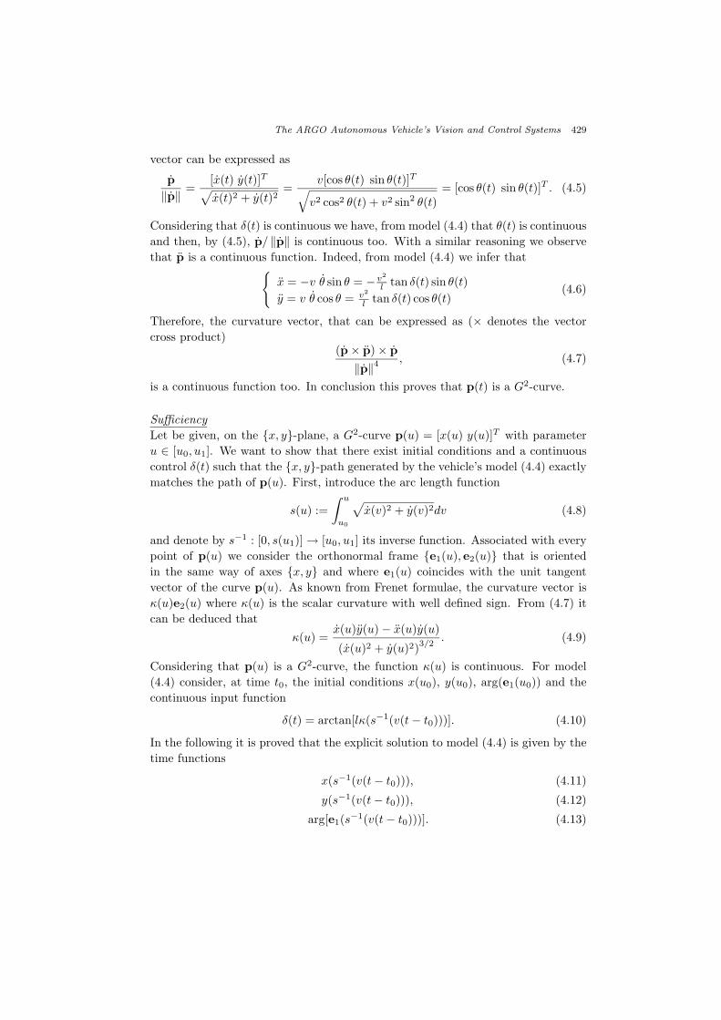
vector can be expressed as

p‖p‖

=[x(t) y(t)]T√x(t)2 + y(t)2

=v[cos θ(t) sin θ(t)]T√v2 cos2 θ(t) + v2 sin2 θ(t)

= [cos θ(t) sin θ(t)]T . (4.5)

Considering that δ(t) is continuous we have, from model (4.4) that θ(t) is continuousand then, by (4.5), p/ ‖p‖ is continuous too. With a similar reasoning we observethat p is a continuous function. Indeed, from model (4.4) we infer that{

x = −v θ sin θ = −v2

l tan δ(t) sin θ(t)y = v θ cos θ = v2

l tan δ(t) cos θ(t)(4.6)

Therefore, the curvature vector, that can be expressed as (× denotes the vectorcross product)

(p× p)× p

‖p‖4, (4.7)

is a continuous function too. In conclusion this proves that p(t) is a G2-curve.

SufficiencyLet be given, on the {x, y}-plane, a G2-curve p(u) = [x(u) y(u)]T with parameteru ∈ [u0, u1]. We want to show that there exist initial conditions and a continuouscontrol δ(t) such that the {x, y}-path generated by the vehicle’s model (4.4) exactlymatches the path of p(u). First, introduce the arc length function

s(u) :=∫ u

u0

√x(v)2 + y(v)2dv (4.8)

and denote by s−1 : [0, s(u1)]→ [u0, u1] its inverse function. Associated with everypoint of p(u) we consider the orthonormal frame {e1(u), e2(u)} that is orientedin the same way of axes {x, y} and where e1(u) coincides with the unit tangentvector of the curve p(u). As known from Frenet formulae, the curvature vector isκ(u)e2(u) where κ(u) is the scalar curvature with well defined sign. From (4.7) itcan be deduced that

κ(u) =x(u)y(u)− x(u)y(u)

(x(u)2 + y(u)2)3/2. (4.9)

Considering that p(u) is a G2-curve, the function κ(u) is continuous. For model(4.4) consider, at time t0, the initial conditions x(u0), y(u0), arg(e1(u0)) and thecontinuous input function

δ(t) = arctan[lκ(s−1(v(t− t0)))]. (4.10)

In the following it is proved that the explicit solution to model (4.4) is given by thetime functions

x(s−1(v(t− t0))), (4.11)

y(s−1(v(t− t0))), (4.12)

arg[e1(s−1(v(t− t0)))]. (4.13)


From standard derivation rules we obtain

d

dt[x(s−1(v(t− t0)))] = v

x(u)‖p(u)‖

∣∣∣∣u=s−1(v(t−t0))

=

= v cos[arg[‖p(u)‖−1 p(u)]

]∣∣∣u=s−1(v(t−t0))

(4.14)

and analogously

d

dt[y(s−1(v(t− t0)))] = v

y(u)‖p(u)‖

∣∣∣∣u=s−1(v(t−t0))

=

= v sin[arg[‖p(u)‖−1 p(u)]

]∣∣∣u=s−1(v(t−t0))

. (4.15)

Considering that e1(u) ≡ ‖p(u)‖−1 p(u), identities (4.14) and (4.15) verify the firsttwo equations of model (4.4). Define as θ(t) the time function appearing in (4.13).Hence, we have

θ(t) =

arctan [y(u)/x(u)]

∣∣∣u=s−1(v(t−t0))

if x(u) ≥ 0

π + arctan [y(u)/x(u)]∣∣∣u=s−1(v(t−t0))

if x(u) < 0(4.16)

and, by derivation, obtain

θ(t) =ddt [y(u)]x(u)− y(u) ddt [x(u)]

x(u)2 + y(u)2

∣∣∣∣∣u=s−1(v(t−t0))

=

= vx(u)y(u)− x(u)y(u)

(x(u)2 + y(u)2)3/2

∣∣∣∣∣u=s−1(v(t−t0))

. (4.17)

Note that, in the definition (4.16) of θ(t) we have assumed

arctan [y(u)/x(u)]∣∣∣x(u)=0

:={

+π/2 if y(u) > 0−π/2 if y(u) < 0 (4.18)

By virtue of (4.9) it is then proved that

θ(t) = v κ(s−1(v(t− t0))). (4.19)

On the other hand relation (4.10) implies

v

ltan δ(t) = v κ(s−1(v(t− t0))) (4.20)

so that (4.19) and (4.20) verify the third equation of model (4.4).From (4.11) and (4.12) we finally note that the {x, y}-path generated by input

(4.10) exactly matches the path of p(u). 2


��

�� !�

"$# ��%'&(��)

*,+.-0/

1�2�3�2�4�56�7 8!79;: 4=<

>

?A@$B�C(DAE�F�?�G�D

HJILKNM�O$P�Q�R�ST S(R�S�U�V W�X�U

Fig. 21. The new recursive trajectory control scheme.

�

�

��

� �

��

��

Fig. 22. The G2-interpolating problem on the {x, y}-plane.

4.3. Quintic G2-splines and Recursive Trajectory Control

The sufficiency proof of Proposition 1 gives the explicit dynamic inversion formulae(4.8)–(4.10) for the open-loop steering control of vehicle (4.4) provided that thedesired path to follow is assigned as a given parametric curve. Therefore, considerthe following interpolating path problem. Let be given on plane {x, y} two distinctpoints pA = [xA yA]T and pB = [xB yB ]T with assigned unit tangent vectorsdefined by θA and θB and scalar curvatures κA and κB (see figure 22). The signsof κA and κB are given according to the Frenet formulae; cf. the introduction to(4.9) in the proof of Proposition 1. The data pA, θA, and κA represent the vehicle’scurrent status at a given time t0, i.e. the coordinates xA and yA of the rear axlemidpoint, the heading angle, and the curvature κA given by

κA = (1/l) tan δ(t0) (4.21)

where δ(t0) is the current steering angle. The data pB , θB , and κB are the desiredfuture status of the vehicle.

The parametric curve to consider is a quintic polynomial vector function p(u) =[x(u) y(u)]T , u ∈ [0, 1] where

x(u) := x0 + x1u+ x2u2 + x3u

3 + x4u4 + x5u

5 (4.22)


y(u) := y0 + y1u+ y2u2 + y3u

3 + y4u4 + y5u

5. (4.23)

with interpolating conditions (cf. (4.5) and (4.9)):

p(0) = pA , p(1) = pB , (4.24)p(0)‖p(0)‖

=[

cos θAsin θA

],

p(1)‖p(1)‖

=[

cos θBsin θB

], (4.25)

κ(0) = κA , κ(1) = κB . (4.26)

Focusing on polynomial parametric curves and working with arbitrary interpolatingdata, it is necessary to use, at least, quintic polynomials as in (4.22), (4.23), in orderto satisfy conditions (4.24)–(4.26).26 Nevertheless, conditions (4.24)–(4.26) leavefour degrees of freedom that are exploited by the following closed-form solution:

x0 = xA (4.27)

x1 = η1 cos θA (4.28)

x2 =12(η3 cos θA − η2

1κA sin θA)

(4.29)

x3 = 10(xB − xA)− (6η1 +32η3) cos θA − (4η2 −

12η4) cos θB

+32η2

1κA sin θA −12η2

2κB sin θB (4.30)

x4 = −15(xB − xA) + (8η1 +32η3) cos θA + (7η2 − η4) cos θB

−32η2

1κA sin θA + η22κB sin θB (4.31)

x5 = 6(xB − xA)− (3η1 +12η3) cos θA − (3η2 −

12η4) cos θB

+12η2

1κA sin θA −12η2

2κB sin θB (4.32)

y0 = yA (4.33)

y1 = η1 sin θA (4.34)

y2 =12(η3 sin θA + η2

1κA cos θA)

(4.35)

y3 = 10(yB − yA)− (6η1 +32η3) sin θA − (4η2 −

12η4) sin θB

−32η2

1κA cos θA +12η2

2κB cos θB (4.36)

y4 = −15(yB − yA) + (8η1 +32η3) sin θA + (7η2 − η4) sin θB

+32η2

1κA cos θA − η22κB cos θB (4.37)

y5 = 6(yB − yA)− (3η1 +12η3) sin θA − (3η2 −

12η4) sin θB

−12η2

1κA cos θA +12η2

2κB cos θB (4.38)


The real parameters ηi, i = 1, . . . , 4, appearing in the above relations, can be packedtogether to form the four-dimensional parameter vector η := [η1η2η3η4]T so thatthe resulting parametric curve be concisely denoted as p(u;η).

Proposition 2 (Guarino Lo Bianco and Piazzi26). Given any interpolatingdata pA, θA, κA and pB , θB , κB , the parametric curve p(u;η) satisfies condi-tions (4.24)–(4.26) for all η1, η2 ∈ IR+ and all η3, η4 ∈ IR. Conversely, given anyquintic polynomial curve p(u) with p(0) 6= 0, p(1) 6= 0 satisfying (4.24)–(4.26)there exists parameters η1, η2 ∈ IR+ and η3, η4 ∈ IR such that it can be expressedas p(u;η).

Note that η1 = p(0;η), η2 = p(1;η) are “velocity” parameters whereas η3, η4

can be denoted as “twist” parameters of the curve. These parameters can be chosenin order to appropriately shape the trajectory, for example minimizing the curvaturein a lane changing maneuver or minimizing the variations of curvature following aroad arc with constant curvature.

The recursive use of the parametric curve p(u;η) permits to exactly interpolateany given sequence of cartesian points with arbitrarily assigned unit tangent andcurvature vectors. In such a way it results an overall G2-curve, i.e. a curve withsecond order geometric continuity. In the following we refer to p(u;η) as the quinticG2-spline.

Figures 21 and 23 help describing the new overall feedforward/feedback controlof the ARGO vehicle on the path following functionality. A new quintic G2-splineis planned at the chosen trajectory updating rate. The vision data system with theIPM can give, on a planar {x, y}-coordinate system, the road scene with knowncar’s position and path to follow. Hence pA and θA are known and the currentcurvature κA of the vehicle path can be computed with relation (4.21).

The interpolating point pB is determined on the path to follow at the interpolat-ing distance ID from vehicle’s rear axle midpoint. The vision data processing shouldalso provide the tangent angle θB with respect to axis x and the path curvatureκB at pB . The supervisor (see figure 21), collect the interpolating data, assign theshaping vector parameter η, and pass all the data to the G2-spline generator. Fromthe knowledge of p(u;η) a dynamic inversion based on model (4.4) is performed viaformulae (4.8)–(4.10) for obtaining the steering angle function

δ(t) = arctan[lκ(u;η)]|u=s−1(v(t−t0)) . (4.39)

In (4.39), κ(u;η) denotes the curvature of the G2-spline p(u;η) and v is the vehiclevelocity that is considered constant during the trajectory updating time, i.e. thetime slot where the steering action (4.39) is based on the updated G2-spline.

The feedback action is issued by the supervisor by planning a new G2-spline, sothat the steering control (4.39) is updated, when the vehicle has covered a relativelysmall fraction of the current G2-spline. This mechanism is recursively applied tothe new G2-spline resulting in an overall continuous steering control that makes thevehicle converging on the desired path.


d��

�

�

��

��

��

��

"!

#%$

&�' (*)+)+,�-.0/ (213,"4 .05*/76

Fig. 23. Vision-based planning of the G2-spline.

4.4. Simulation Results

The new flatness-based recursive trajectory control scheme, shown in figure 21, hasbeen simulated. To obtain realistic results, the Wong car lateral model has beenadopted.27 It takes into account the geometric and dynamic characteristics of thevehicle as well as the tires characteristics. A summary of the model parametersis reported in tab. 2. In that table m indicates the vehicle mass, J the inertiawith respect to the center of gravity, lf and lr indicate the distance of the centergravity with respect to the front and the rear wheels respectively, Cf and Cr arethe cornering stiffness of the front and the rear wheels and µ is the coefficient ofroad adhesion (µ = 1 for dry roads). It has been supposed that the frame rateof the visual system is the same of the proportional controller currently used inthe ARGO vehicle: 50 Hz. The delay time from the image acquisition to thecontrol actuation has been considered in the simulations. A reasonable value of0.008 s, deduced from the gain scheduled proportional controller used by real ARGOvehicle, has been adopted. The supervisory controller renews the spline coefficientswith a rate that is a fraction of the frame rate. The reason for this choice isintrinsic to the selected control strategy. In fact, to correctly approach the desired


Table 2. Parameters for the simulated car.

m = 1300 kgJ = 2900 kg m2

lf = 1.15 mlr = 1.52 mCf = Cr = 45000 N rad−1

µ = 1

road path, a proper percentage of the spline path must be covered before it isupdated. Practically, we have a spline updating rate equal to 50/ν with ν beinga positive integer. The parameter ν is selectable and is chosen to obtain the bestperformance from the controlled system. Normally, the spline updating rate haveto be increased proportionally with the car speed. Also the interpolating distanceID, i.e. the ahead distance used to plan the spline, is proportional to the vehicle’svelocity in a way similar to (4.1). Vector η has been chosen to guarantee thegeneration of optimal trajectories in the cases of lane change, straight roads orcurves with small curvatures (the curvature range considered practically covers allthe standard highways curvatures). “Optimal” means that the error between thegenerated spline and the road path is minimum and, at the same time, this result isobtained with minimum variations of the steering command δ.26 Roads with verylarge curvatures requires different values for η. A suboptimal behaviour must beexpected for sharp curves because in this simulations η is supposed to be constant(η = [25 25 −45 45]T ) .

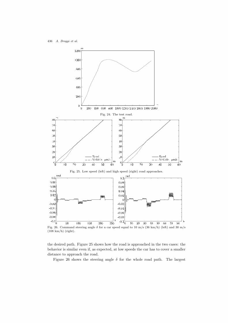
The simulation results reported in the following refer to the road shown infigure 24. It is composed by a sequence of line segments and circular arcs joined toobtain an overall G1-path (cf. subsection 4.2). The road shape, that is discontinuousat segment/arc joints, complicates the control task because the controller alwaysplans trajectories with continuous curvatures. Road curvatures are chosen insidethe interval [0, 0.005] m−1. The maximum curvature (corresponding to 200 m ofradius) is bigger than standard highway curvatures: the purpose is to test thecontrol strategy in critical situations, i.e. when the chosen value of η is not themost appropriate.

Two different car speeds have been used for the simulations. In the first run aconstant velocity of 10 m/s (36 km/h) has been chosen, while in the second run thevelocity has been increased to 30 m/s (108 km/h). In the first simulation ν wasfixed equal to 30 (which corresponds to a spline update time of 0.6 s) while in thesecond one it was decreased to 10 (spline update time equal to 0.2 s). Owing to theWong’s model used to describe the car, the actual car paths are different for thetwo cases, but in both situations the maximum tracking error is smaller than 20 cmand it occurs when the curvature radius of the road becomes equal to 200 meters.On the straight stretches the error is very close to zero.

At the beginning, if the vehicle is not on the correct path, it converges toward


� �� !�!#"�$�$�$%

&�'�'

(�)�)

*�+�+

,�-�-

.�/�/�/

0�1�2�2

3

4

Fig. 24. The test road.

� ��

��

��

��

��

��

��

"!

#�$ %

&')(�*,+ -�. (0/21435*687�9�:

� ��

��

��

��

��

��

��

"!

#�$ %

&')(�*,+ -�. (0/21435*687�9�:

Fig. 25. Low speed (left) and high speed (right) road approaches.

� ��

�� !"�# "$%�& ')(+*�,

-. /0 1322 4356 788 9:; � �� !#"�$ "�%&#'�( '�)*�+�, +.-/�0�1 0�2

34�5 4�67�8 7.9:�; :�<=�> =�?@�A B CED�F

GFig. 26. Command steering angle δ for a car speed equal to 10 m/s (36 km/h) (left) and 30 m/s(108 km/h) (right).

the desired path. Figure 25 shows how the road is approached in the two cases: thebehavior is similar even if, as expected, at low speeds the car has to cover a smallerdistance to approach the road.

Figure 26 shows the steering angle δ for the whole road path. The largest


steering angle is detected at the beginning of the simulation when the vehicle has toapproach the road, but even in that case it is smaller than 0.1 rad (close to 5o). Asexpected, the worst situation for the control algorithm is detected when the vehicleapproaches curves with the biggest curvature (0.005 m−1). Nevertheless, in theworst case (i.e at low speed) the steering command δ has a peak-to-peak amplitudeequal to 0.02 rad (1o). In future works, the performances will be further improvedby considering a variable η, chosen depending on the road curvature.

5. Results

The following paragraphs present a 2000 km test on the road. For each systemcomponent a detailed analysis of the main problems encountered during the test ispresented and the overall system performance is discussed.

5.1. The MilleMiglia in Automatico Tour

In order to extensively test the Road Following functionality under different trafficsituations, road environments, and weather conditions, a 2000 km journey was car-ried out in June 1998 along the Italian highway network. The Italian road networkis particularly suited for such an extensive test since it is characterized by quicklyvarying road scenarios including different weather conditions and a generally largeamount of traffic. During the journey, besides the usual tasks of data acquisitionand processing for automatic driving, the system logged the most significant data,such as speed, position of the steering wheel, lane changes, user interventions andcommands, and dumped the whole status of the system (images included) in cor-respondence to situations in which the system had difficulties in reliably detectingthe road lane.

After the end of the tour, the collected logs have been processed in order tocompute the overall system performance, such as the percentage of automatic driv-ing, and to analyze unexpected situations. At the end of the tour, the system logscontained more than 1200 Mbyte of raw data.

5.2. Performance Analysis

5.2.1. The Vision System

The low-cost cameras installed on the ARGO vehicle demonstrated to be the weak-est component of the whole system. Although they have a high sensitivity even inlow light conditions (e.g. the twilight), a quick change in the illumination of thescene causes a degradation in the image quality. In particular, in correspondenceto a tunnel exit images are completely saturated for about 100÷200 ms thereforenullifying the processing. The use of cameras featuring automatic gain control andhigher dynamics is now under evaluation.


5.2.2. The Processing System

The processing system installed on ARGO during the tour was a a commercialPC with a 200 MHz Pentium processor and 32 Mbyte of memory. It was able toprocess up to 25 pairs of stereo frames per second and provide the control signals forautonomous steering every 40 ms (e.g. one refinement on the steering wheel positionfor every meter at 100 km/h), proving to be powerful enough for the automaticdriving of the vehicle.

5.2.3. The Visual Processing

The IPM approach used for Lane Detection, proved to be effective for the wholetrip. Even if on Italian highways the flat road assumption is not always valid,anyway, the approximation of the road surface with a planar surface was acceptable.The wrong calibration, in fact, generates a lateral offset in the vehicle trajectory.Nevertheless, since the highway lanes’ width is sufficiently large, this offset hasnever caused serious problems. Anyway, an enhancement to the IPM transform iscurrently under development.28

5.2.4. The Control System

The control system tested during the tour was based on the gain scheduled propor-tional controller previously discussed. With this kind of control, for speeds reachingaround 90÷ 95 km/h there was no noticeable difference in comparison to a humandriver, while for higher speeds (up to 123 km/h) the vehicle tended to oscillateinside the lane.

Regarding the mechanical part, an electric stepping motor allows the rotationof the steering wheel with a high resolution and a reduced power consumption.

5.2.5. Environmental Conditions

During the tour, the system’s behavior was evaluated in various environmental con-ditions. The route was chosen in order to include areas with different morphologicalcharacteristics: from flat areas to sloping territories of the Appennines region andheavy traffic zones, inevitably encountering stretches of highway with road works,absent or worn horizontal road signs, and diversions, and various weather condi-tions. The different environmental conditions demonstrated the robustness of theimage processing algorithms.

5.2.6. Statistical analysis of the tour

The analysis of the data collected during the tour29 allowed the computation of anumber of statistics regarding system performance (see table 3). The automaticdriving percentage and the maximum distance automatically driven show high val-ues despite the presence of many tunnels and of several stretches of road with absentor worn lane markings or even no lane markings at all.


Table 3. Statistical data regarding the system performance during the tour.

Maximum distance in automatic [km]Percentage of automatic drivingMaximum speed [km/h]Average speed [km/h]km

Stage Departure Arrival

1 Parma → Turin 245 86.6 109 93.3 23.42 Turin → Pavia 175 80.2 95 85.1 42.23 Pavia → Ferrara 340 89.8 115 86.4 54.34 Ferrara → Ancona 260 89.8 111 91.1 15.15 Ancona → Rome 365 88.4 108 91.1 20.86 Rome → Florence 280 87.5 110 95.4 30.67 Florence → Parma 195 89.0 123 95.1 25.9

It is important to note that some stages included passing through toll stationsand transiting in by-passes with heavy traffic and frequent queues during which thesystem had to be switched off.

6. Conclusions and Future Work

The experience gained during these years of work within the ARGO project clearlyhighlighted some of the main problems of automatic driving, whilst the extensiveuse of the ARGO prototype helped to find their most promising solutions.

The main aims established at the beginning of the project were achieved, namelythe development of a prototype vehicle and its use as a test-bed for both the hard-ware and software aspects of the project.

The critical analysis of the results of the MilleMiglia in Automatico tour, aswell as the experience gained during the last few years, will be helpful for the futureresearch within the ARGO project, namely the development of a new vehicle whichwill include the automatic control of both the steering wheel and the speed. Newand more robust algorithms for Vehicle Detection are currently under developmentas well as a new module for Pedestrian Detection.

Also the control subsystem will derive benefit from the new strategies high-lighted in this work: the expected advantages of the new flatness-based recursivetrajectory control over the previous proportional control are basically: (i) superiorroad following with smooth cruising and (ii) highly-flexible functionality. In par-ticular flexibility can be simply obtained by modifying the supervisor strategy inorder to perform, for example, lane changing, lane inserting, platooning and evencar parking maneuvers.

References

1. A. Broggi, M. Bertozzi, A. Fascioli, and G. Conte, Automatic Vehicle Guidance: theExperience of the ARGO Vehicle, World Scientific, Apr. 1999. ISBN 981-02-3720-0.


2. R. Frezza, S. Soatto, and G. Picci, “Visual path following by recursive spline updating,”in Proceedings of the 36th Conference on Decision and Control, pp. 1130–1134,(San Diego, California USA), Dec. 1997.

3. Y. Ma, J. Kosecka, and S. Sastry, “Vision guided navigation for a nonholomonic mobilerobot,” IEEE Transaction on Robotics and Automation 15(3), pp. 521–536, 1999.

4. C. Hatipoglu, K. Redmill, and U. Ozguner, “Steering and lane change: a workingsystem,” in IEEE Conference on Intelligent Transportation Systems, ITSC’97,(Boston, MA), Nov. 1997.

5. C. J. Taylor, J. Kosecka, R. Blasi, and J. Malik, “A comparative study of vision-basedlateral control strategies for autonomous highway driving,” The International Journalof Robotic Research 18(5), pp. 442–453, 1999.

6. H. Peng and M. Tomizuka, “Lateral control of front-wheel steering rubber-tire vehicles,”Tech. Rep. UCB-ITS-PRR-90-5, Institute of transportation studies, Berkeley, CA, 1990.

7. R. E. Parson and W. B. Zhang, “Program on advanced technology for the highwaylateral guidance/control,” in Proc. of the 1st Int’l Conf. Applications of advancedTechnology in Transpotation Engineering, pp. 275–280, (San Diego, CA), 1989.

8. W. Zhang, R. E. Parsons, and T. West, “An intelligent roadway reference system for ve-hicle lateral guidance/control,” in Proc. of the 1990 American Control Conference,ACC90, pp. 281–286, (San Diego, CA), 1990.

9. N. Matsumoto and M. Tomizuka, “Vehicle lateral velocity and yaw rate control with twoindependent control inputs,” in Proc. of the 1990 American Control Conference,ACC90, pp. 1868–1875, (San Diego, CA), 1990.

10. T. Hessburg and M. Tomizuka, “Fuzzy logic control for lateral vehicle guidance,” IEEEControl System Magazine 14, pp. 55–63, Aug. 1994.

11. J. Ackermann and W. Sienel, “Robust control for automated steering,” in Proc. of the1990 American Control Conference, ACC90, pp. 795–800, (San Diego, CA), 1990.

12. J. Ackermann, “Robust car steering by yaw rate control,” in Proc. of the 1990 Con-ference on Decision and Control, CDC90, pp. 2033–2034, (Honolulu), 1990.

13. J. Ackermann, Robust Control: systems with uncertain phisical parameters, Com-munications and Control Engineering, Springer-Verlag, London, Great Britain, 1993.

14. R. H. Byrne, C. T. Abdallah, and P. Dorato, “Experimental results in robust lateralcontrol of highway vehicles,” IEEE Control Systems 18(2), pp. 70–76, 1998.

15. B. Epiau, F. Chaumette, and P. Rives, “A new approach to visual servoing,” IEEETrans. on Robotics and Automation 8(3), pp. 313–326, 1992.

16. D. Pomerleau, “Progress in neural network-based vision for autonomous robot driving,”in Proc. of the Int. Vehicles ’92 Symposium, pp. 391–396, (Detroit), 1992.

17. D. Pomerleau, “RALPH: Rapidly adapting lateral position haldler,” in Proc. of theInt. Vehicles ’95 Symposium, pp. 54–59, 1995.

18. U. Ozguner, K. Unyelioglu, and C. Hatipoglu, “An analytical study of vehicle steer-ing control,” in Proc. of the IEEE Conf. on Control Applications, pp. 125–130,(Washington, DC), 1995.

19. S. Tsugawa, H. Mori, and S. Kato, “A lateral control algorithm for vision-based vehicleswith a moving target in the field of view,” in 1998 International Conference onIntelligent Vehicles, vol. 1, pp. 41–45, (Stuttgart, Germany), Oct. 1999.

20. M. Fliess, J. Levin, P. Martin, and P. Rouchon, “Sur les systemes non lineairesdifferentiellement plots,” C. R. Acad. Sci. Paris I–315, pp. 619–624, 1992.

21. M. Fliess, J. Levin, P. Martin, and P. Rouchon, “Flatness and defect of nonlinearsystems: introduction theory and examples,” Int. J. of Control 61(6), pp. 1327–1361,1995.

22. J. Levine, “Are there new industrial perspectives in the control of mechanical sys-


tems?,” in Advances in Control: highlights of ECC’99, P. M. Frank, ed., pp. 197–226,Springer-Verlag, (London, Great Britain), 1999.

23. P. Rouchon, M. Fliess, J. Levin, and P. Martin, “Flatness, motion planning and trailersystems,” in Proceedings of the 32nd IEEE Conference on Decision and Control,CDC’93, pp. 2700–2705, 1993.

24. P. Rouchon, M. Fliess, J. Levin, and P. Martin, “Flatness and motion planning: thecar with n trailers,” in Proceedings of the European Control Conference, ECC’93,pp. 1518–1522, (Groninger, Netherlands), 1993.

25. B. A. Barsky and J. C. Beatty, “Local control of bias and tension in beta-spline,”Computer Graphics 17(3), pp. 193–218, 1983.

26. C. Guarino Lo Bianco and A. Piazzi, “Quintic G2-splines for trajectory planning ofautomated vehicles,” Tech. Rep. TSC03/99, Dip. Ingegneria Informazione, Universityof Parma, Parma (Italy), Oct. 1999.

27. J. Wong, Theory of ground vehicles, John Wiley & Sons Inc., New York, 2nd ed.,1993.

28. M. Bertozzi, A. Broggi, and A. Fascioli, “An extension to the Inverse Perspective Map-ping to handle non-flat roads,” in Procs. IEEE Intelligent Vehicles Symposium‘98,pp. 305–310, (Stuttgart, Germany), Oct. 1998.

29. A. Broggi, M. Bertozzi, and A. Fascioli, “The 2000 km Test of the ARGO Vision-BasedAutonomous Vehicle,” IEEE Intelligent Systems 14, pp. 55–64, Jan.–Feb. 1999.

Documents

THE ARGO AUTONOMOUS VEHICLE’S VISION AND ... Journal of Intelligent Control and Systems Vol. 3, No. 4 (1999) 409{441 c World Scienti c Publishing Company THE ARGO AUTONOMOUS VEHICLE’S