Embed Size (px)
Citation preview
The Approach of using Molecular Dynamics for
Nanofluid Simulations
Adil Loya1, Jacqueline L. Stair
2, Guogang Ren
1
1School of Engineering and Technology, University of Hertfordshire
2School of Pharmacy, University of Hertfordshire
Hatfield
United Kingdom
Abstract—The approach of using molecular dynamics (MD)
for mimicking the dynamics of nanoparticles dispersion in
different fluids is increasing since last decade. This vast
increment utilizes computational softwares to mimick distictive
aspects of experimental conditions. The technique of MD further
makes it easier for understanding conditions of physical and
chemical interactions that exist in nanofluid system.
However, this review explains the procedure and implication
on how to simulate the nanofluid system using molecular
dynamics. Further, it is made easier for the reader for applying
the technique, by good software recommendations and step by
step procedure are given for utilization of successful nanofluid
simulations.
Keywords—Nanofluid; Molecular dynamics; Brownian;
Diffusion; Dispersion.
I. INTRODUCTION
The word nanofluid, explains itself, assuming nano as a system that is specified at the level of 10
-9m, and fluid as the
form of matter that continually deforms itself under applied shear stress. The application of nanoparticles as a carrier medium in fluid produces nanofluid. This nanofluid consists of particles that exhibit Brownian motion when they are dispersed in the fluid. The use of nanoparticle enhances the properties of the fluid. These properties are physical[1, 2], rheological[3-6], electrical[7], chemical[8, 9] and biological[10-12].
There has been lots off nanofluids experimental studies. These studies are related to metal, metaloxides, ceramic and polymeric nanoaprticles dispersion in different base fluids. The nanofluid experimental studies have tried to undermine different properties of basefluid modification with nanoparticles. These properties are thermal conductivity enhancement, viscosity change, particle sizes, zeta potential, density, heat capacity, heat flux, electrostatic and Van der Waal forces, pH variation, and many others. Variable parameters are too many and increases with changing nanoparticles being used. The extent of extracting different parameters with experimentation requires high technical expertise, as well as, requires extensive material usage for accuracy of data prediction and extensive time period for performing each experiment.
Different experimental studies for nanofluids have been done for more than two decades. The Argonne Lab in United
States under the supervision of Dr. Stephen US Choi was the first to call new heat transfer fluid as ―Nanofluids‖[13, 14]. Further, various researchers started to undermine distinctive properties of nanofluids in different conditions. The outbreak of usage was not just held in the engineering sciences; whereas, it became popular in biological science and pharmacology. The enhancement of the properties was immense as compared to the amount of particle concentration being used. The investigated study shows that Al2O3 nanoparticles when used at a volume fraction of 1-5%, shows 60% increment in the viscosity of water[15]. Then CuO nanoparticles have been investigated showing an increase of viscosity by 60-80% in water based nanofluid[16]. Later other nanoparticles were also examined for enhancing viscosity, thermal conductivity and other proeprties[17-21]. The usage of nanoparticles in biological basefluids enhances the properties of fluid. This nano-biofluid received a huge importance from the medical side for diffusing the Gold nanoparticles in different fluids to treat cancers[10].
However, as discussed that there have been immense experimental studies on the dispersion and application of nanofluids; nevertheless, conducting these experiments is being considered as an expensive and time consuming method. Further, predicted experimental results are genuine, on the contrary, they require lots of effort and knowledge on experimental procedures. Due to these drawbacks and upcoming computer age, researchers are more diverting the experimentation on simulation platforms. Therefore, since the last decade due to enhancements in molecular dynamics and computational technology, nanoparticle dispersions in different fluid‘s simulation are being attempted. By conducting the dispersion of nanoparticles in fluid using MD has become a useful and cost-effective approach. MD has become popular for nanofluids simulation on a large scale since the last decade as tabulated in table2. Before this, there were MD simulations, but they were mostly related to self-diffusion of fluids[22], mixing of oil with water to create emulsions, protein bi-layer [23]and polymeric diffusions [24].
The increase in the nanofluidic simulations is due to the concern and curiosity of how the diffusion of nanoparticles takes place in different fluids. These simulations can easily be used to understand the pheonomena and further analysis. The electrostatic, Van der Waal, electrosteric and Derjaguin and Landau, Verwey and Overbeek (DVLO) theory can further be understood by simulation, which were hard to understand at the
1236
International Journal of Engineering Research & Technology (IJERT)
IJERT
IJERT
ISSN: 2278-0181
www.ijert.orgIJERTV3IS051461
Vol. 3 Issue 5, May - 2014
time of experimental studies. Moreover, the visualization of the simulations can explain the transport of the nanoparticle in fluid on the greater scale; this is a necessary fact to understand the diffusion of nanoparticles, since it differs from its microparticles counterparts. Thereby, lots of researchers came up with different techniques to design nanoparticles fluid interactions; some came up with their own potential and some used already available techniques. Nevertheless, these applied techniques and methods were progressive in describing the nanoparticle interaction with different fluids. Furthermore, researchers have also tried to use various simulation packages.
The initiative was mostly started with describing the system dispersion and diffusion with the Brownian equation of motion that is interconnected with Einstein diffusion model as shown in equation 1 and 2.
Later, Stokes formulation was also incorporated for enhancing the results. Moreover, the derivation for Newton‘s formulation indeed starts from the Langragian formulation that was further optimized by the Galilean relativity principle. This derivation is the bases for the molecular dynamic simulations to analyze the detailed atomic motion within the MD domain rather than just implementing the statical analysis [25]
i i iF m a (1)
(2)
Fi force on particle i, mi mass of particle i, ai acceleration of
particle i, r is the position vector and V is the potential energy
derivative. Equations of motion are time reversible; if we
change the signs of all velocities, the atoms will retrace their
trajectories. Furthermore, numerical methods are required to
solve these equations for systems larger than two independent
particles.
However, this review demonstrates the simplicity for adopting the MD technique for nanofluid simulations. Further it describes to the reader, the easy procedure for carrying out these simulations. There are different reviews on MD, but they are mostly oriented towards biological or protein simulations. Further, this review has gathered previous studies carried out by others on various nanofluid simulations using different methodologies as shown in table 2.
II. SIMULATION METHODOLOGY
The process followed by the molecular dynamic simulation
technique equilibrate the system from its unstable position to
stable position. Implementing force field causes the movement
of the atoms in the system. Later, the pair potential, computes
a particular behavior that is required to fulfil the simulation.
The movement of particles in the system is caused by the
velocity theorem, i.e. carried out by ensembles. These
ensembles help to carry out thermodynamic conditions on a
system using the kinetic theory of a molecular system; this
theory further causes the system equilibration with time
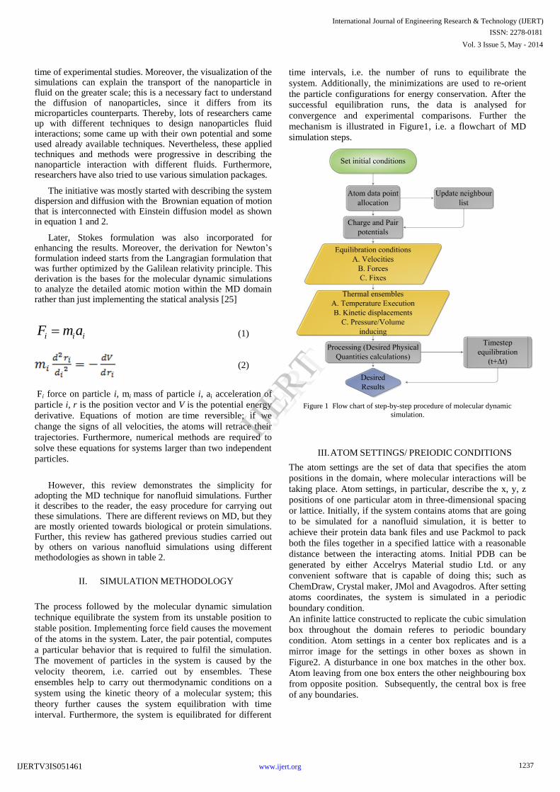
interval. Furthermore, the system is equilibrated for different
time intervals, i.e. the number of runs to equilibrate the
system. Additionally, the minimizations are used to re-orient
the particle configurations for energy conservation. After the
successful equilibration runs, the data is analysed for
convergence and experimental comparisons. Further the
mechanism is illustrated in Figure1, i.e. a flowchart of MD
simulation steps.
Figure 1 Flow chart of step-by-step procedure of molecular dynamic
simulation.
III. ATOM SETTINGS/ PREIODIC CONDITIONS
The atom settings are the set of data that specifies the atom
positions in the domain, where molecular interactions will be
taking place. Atom settings, in particular, describe the x, y, z
positions of one particular atom in three-dimensional spacing
or lattice. Initially, if the system contains atoms that are going
to be simulated for a nanofluid simulation, it is better to
achieve their protein data bank files and use Packmol to pack
both the files together in a specified lattice with a reasonable
distance between the interacting atoms. Initial PDB can be
generated by either Accelrys Material studio Ltd. or any
convenient software that is capable of doing this; such as
ChemDraw, Crystal maker, JMol and Avagodros. After setting
atoms coordinates, the system is simulated in a periodic
boundary condition.
An infinite lattice constructed to replicate the cubic simulation
box throughout the domain referes to periodic boundary
condition. Atom settings in a center box replicates and is a
mirror image for the settings in other boxes as shown in
Figure2. A disturbance in one box matches in the other box.
Atom leaving from one box enters the other neighbouring box
from opposite position. Subsequently, the central box is free
of any boundaries.
1237
International Journal of Engineering Research & Technology (IJERT)
IJERT
IJERT
ISSN: 2278-0181
www.ijert.orgIJERTV3IS051461
Vol. 3 Issue 5, May - 2014

Figure 2 Periodic boundary replication.
IV. FORCE FIELDS
The force field is a basic step to describe the interactions
between atoms and their potential energies. Furthermore, force
fields can be constructed by parameters achieved from the
potential energies using the apparatus such as experimental
data of x-ray electronic diffraction, Nuclear magnetic
resonance (NMR) and Fourier‘s transformation infrared
(FTIR) spectroscopy; which gives the differentiation between
matter and radiation with the uses of semi-experimental
technique of quantum-mechanical calculation. Moreover,
force fields are obtained parameters from higher-level
quantum-mechanic calculations. These calculations help in
imitating the realistic performance of the atomistic system
with which results of interactions can be achieved in a matter
of time. However, a successful simulation performance
depends on the rationality of force fields being used.
Further, the computation of classical energy terms is carried
out using force field. These terms account for the calculation
of interaction parameters as shown in Equation 3. Later, this
equation is elaborated for further understanding by graphical
representation as shown in table1, with its specific variable
descriptions.
(3)
The scientific calculation of parameters such as k-bond, k-
angle, and k-torsion are known as potential energy
functions[23]. The subject in simulation depends on its force
field, on the other hand, the way which van der Waals and
electrostatic interaction are treated, determines the precision of
the computational simulation. Additionally, the force fields
that have generally been used are ‗Amber, CHARMM, OPLS
and Gromos‘.
However, for the interatomic collisions, force field
implements interaction parameters of scientific measurements
used to show the potential energy arrangement of elements. To
sum up, force field actually holds parameters that are
controlled from equally experimental observation and large
amount of quantum-mechanics calculation.
The interacting bond expressions are well explained by the
non-bonded van der waals and coulomb‘s forces between the
atoms. The angles terminologies and torsion technique may be
implemented to the corresponding angular coordinates from
the stationary point of a classical diffusion equation. However,
terminologies represent a different primary condition for
diffusion. In addition, the variety of potentials states the
degree of diffusion space in a system. On the other hand,
another method to compute the diffusion coefficient for each
terminology are outlined by interaction potential. Non-bonded
force parameters of larger range interactions can be estimated
from the comparative values of the experimental work for the
Van der Waal and coulomb's parameters.
There are many force fields that give suitable parameters for
mimicking the realistic effect of nanofluid, out of which some
are aimed at each and individual atom in a system. However,
other relate to the whole molecular arrangement. Furthermore,
different types of force fields that has been used and are being
used for nanofluid simulations are given in section 3.A.
A. Types of Force Fields
There are many force fields that are widely being used for
nanofluids such as amber, charmm, compass, opls, gromos,
COMPASS, EAM and MEAM.
A.1 Universal Forcefield(UFF):
Most particles have a force field that gives a parameter aimed
at each and individual molecule in a system. If, integrating
hydrogen with combined atoms of carbon, force fields that
handles hydrogen and carbon atoms in each part of methyl are
controlled by Universal force field. This is a force field
distinctive from others, as it covers all the periodic table
elements. The parameters are an estimation from general rule;
that is used to convert the elemental parameters into
intermolecular interaction parameteric values for calculation.
It is hard to obtain consistensy of results using UFF to that
of experimental ones. Therefore, it is not convenient to use
this force field for condensed state calculations. Nevertheless,
this forcefield is good for exotic molecules for which other
forcefield can not be implemented.
A.2 Amber:
Amber forcefield full abbreviation is Assisted Model Building
Energy Refinement, which is a model created with energy
refinement. Also a collective property of package that agrees
us to convey out MD simulatons. Amber has a set of
molecular mechanical force boundary conditions of bio-
molecule. However, to use AMBER force field it is vital you
have the dimensions for the parameters regarding the force
field. Additionally, it is necessary to check on the charges of
the atoms and force constant. Further, Fig.3 shows the use of
AMBER forcefield to simulate stacked pyrenes that was
carried out by S.M. Langenegger et al.
2 2
0 0 0,
12 6
0, 0,
,
1 1( ) ( ) 1 cos[ ( )]
2 2 2
[ 2 ]
nr i i i
bonds angles torsions
i j ij ij
ij ij
elec Pairs ijij ij ij
VU k r r k n
q q r r
r r r
1238
International Journal of Engineering Research & Technology (IJERT)
IJERT
IJERT
ISSN: 2278-0181
www.ijert.orgIJERTV3IS051461
Vol. 3 Issue 5, May - 2014

Figure 3 AMBER Molecular model of the duplex 3c*4c with two interstrand
stacked pyrenes (HyperChem2 7.0, minimised with amber force field).15 The
nonnucleosidic building blocks are highlighted in red and green. Left: view
perpendicular to the helical axis. Right: view along the helical axis. Showing
the pyrenes stacked on the nucleotide bases; nucleotides on the viewer‘s side have been omitted for clarity; the GC-base pair adjacent to the pyrenes is
shown in blue [26].
A.3 Chemistry At Harvard Macromolecular Mechanics
(CHARMM):
CHARMM that consumes several properties of charm force
fields such as CHARMM19, CHARMM22, and CHARMM27.
In molecular dynamic these are the most popular types of
charm force field. This force field helps in protein
simulations[27]. Later, it was also used for gold nanoaprticles
simulation with peptides[28]. Furthermore, these are mostly
used for protein system, but the drawback of this force field is
it can calculate non-bonded parameters.
A.4 Condense Optimized Molecular Potentials for Atomistic
Simulation (COMPASS):
Moreover, COMPASS is a unique technique which is
considered as a force field that provides atomistic simulation
for reduced materials. Compass means condense optimized
molecular potentials for atomistic simulation[29, 30]. These
force fields permit perfect concurrent estimation of structural,
conformational, vibrational and a thermo physical property
which may occur for a vast range of molecular separation in
condensed phases, and with a confined range of
environments[31]. Later, Fig.4 a,b shows the use of
COMPASS force field for phenol and carboxylic andhydride
simulations [32] and Fig.4c demonstrates the use of this
forcefield in simulating metaloxide nanoparticles in aqueous
fluid[33]. Further the use of COMPASS forcefield for
molecular dynamics of polymer metaloxide system was also
proposed by Prathab et al. [34] .
Figure 4 (a)A close-up view of H-bonding between a phenol group and a carboxylic anhydride group as predicted from the MD simulations of soot
with the COMPASS forcefield; b) MP2/ 6-31G* calculation of H-bonding
between phenol and carboxylic anhydride used to test the result of the
COMPASS-based MD simulation shows similar H-bonding behavior [32];c)
CuO (metaloxide) nanoparticles simulated using COMPASS forcefield[33].
A.5 Optimized Potentials for Liquid Simulations (OPLS):
OPLS is a force field which is divided into two different
sections one being united atom which stands for OPLS-UA
and the other being OPLS-AA force fields. However, the basic
definition of OPLS is optimized potential for liquid
simulations. OPLS-AA force field is used for renovating the
Fourier torsional coefficient. This renovates the accurate data
as an aim proficient fitting subspace of the entire potential
energy surface. Thus, setting weights for each of the fitting
focuses dependent upon sizes of the potential-energy slope.
OPLS-UA [35] is use for possible flattening in standard OPLS-
UA constraint with modification to Van der Waal forces and
improper torsion terms.
A.6 Gromos
Gromos is a general force field that holds information of
biological molecules in a process[36]. Furthermore, it
integrates its specific force field maintaining protein,
nucleotides and so forth. It can be utilised to chemical and
physical nature ranging from glasses and liquid crystal to
polymer and solution of biological particles. This force field is
highly fast due to algorithms as it runs accumulates times
faster than other force feilds.
The Gromos force field vary between the rests in the way
hydrogen atoms are preserved. Furthermore, in the gromos
1239
International Journal of Engineering Research & Technology (IJERT)
IJERT
IJERT
ISSN: 2278-0181
www.ijert.orgIJERTV3IS051461
Vol. 3 Issue 5, May - 2014

force field‘s non-polar hydrogen atoms are reviewed into their
adjacent carbon molecule, i.e. a three particle H-C-H
combination, which formally becomes a single CH2 molecule.
Moreover, this form of force field is called a combined atom
and is more effective for simulation of lipid membrane.
A.7 Embedded Atom Model/Modified (EAM/MEAM)
EAM is a force field that describes and estimates the energy
between two atoms. In this case energy can be known as a sum
of a function of departing between two atoms and its
neighbours in the system. Furthermore, EAM is mostly
associated for a metallic process and is very commonly used
in molecular dynamics simulation[37].
Moreover, the modification of EAM has already been carried
out as MEAM, which stands for modified embedded atom
method. This forcefield is a semi practical derivation method
developed to calculate the properties of a metallic process.
Additionally, this technique has demonstrated to be accurate in
terms of prediction bulk and surface properties within metals.
Modern modification of this forcefield has helped to use large
atoms and elements in the system.
V. PAIR POTENTIAL
Pair potential is a process where a function portrays potential
energy of two particles in interaction. Furthermore, Pair
potentials interlinks with one law which is recognised by
lennard-Jones potentials law denoted by equation (4).
A. Lenard Jones(LJ) Pair potential
LJ potential is an estimation which portrays the potential of
interaction among two non-bonding particles in respect to the
distance of distribution of atoms. Atoms that consist of same
mass and molecular diameter interact by Lennard-Jones
potentials.
12 6
4 ij
ij ij
J cr r
; i,j=[1,2,3,…](4)
Where J is intermolecular potential between two atoms.
ԑ is how strong the particles are attached.
𝜎 is how close they can approach each other.
r is the distance of distribution of particles. Consequently, LJ
potential has many drawbacks that can either put the
simulation in danger or enable to give you the perfect results.
Such as, it only has two parameters, therefore can only be
accumulated into only two physical quantities. Eventually, this
can be an issue to satisfy three different interacting atoms in
the system. As the scaling of energy and bond elasticity after
considering this ideology is difficult to pair all three quantities
together with L-j potential.
B. Brownian potential
Brownian potential is the random motion of molecules
projected in a liquid [38] leading to their collision with fast
atom in solid and liquid state. This potential can be devoted to
mathematical model in simulation to configure the random
movement. Brownian potential also describes the diffusive
limit of the Langevin equation where the motion is highly
random. However, this potential has a high friction coefficient.
Brownian helps in expressing processes as diffusion controlled
system.
C. Smoothed Particle Hydrodynamic (SPH) potential
SPH is an abbreviation for Smoothed Particle Hydrodynamic
which is a computational technique used for the simulation of
fluid hydrodynamics[39, 40]. Furthermore, it applies mesh
free method, where motion is not restricted. In simulation of
fluid dynamics this is highly used, as SPH assures
conservation of mass without further computation since the
molecules state the mass itself. Moreover, it has a feature
which computes pressure from weighted pressure distribution
of neighbouring function rather than solving linear parts of the
system. Furthermore, this potential promotes hydrodynamic
effect in the system. Thus, fulfilling the hydrodynamic
movement of molecules according to the liquid-liquid
layering[41].
D. Dissipative particle dynamic (DPD) potential
DPD is used to perform stochastic simulations [42, 43]. This
potential helps in simulating Brownian dynamics of complex
fluid system. This method was used to neglect lattice
properties for the lattice gas automata and attempt
hydrodynamic time and space with in molecular dynamic
boundaries. Furthermore, DPD involves a set of molecules
moving in the continuous scale of the time and space.
Momentum of conservation of energy necessitates that random
forces applied when two beads are not symmetrical.
Moreover, pairs of molecules interacting take the help of a
single random force calculation. This differentiates DPD to
Brownian dynamics in how each individual particles
experiences random force independently of all molecules.
Additionally, two particles get so close they can be considered
to be known as zero potential energy. Moreover, the space of
distribution decreases as the chances of interaction increased
and in some way the potential is decreased from zero to
negative as the particles held together. However the length
among the base will remain constant to reduce the atoms to
gain a balance which can be estimated by the separation
distance, these values are used for acquiring coefficient of pair
potentials.
VI. ENSEMBLES
Molecular dynamics simulation is attempted under pre-defined
thermodynamic conditions, such as constant number of
particles (N), volume (V), pressure (P) and temperature.
These conditions specify the ―ensemble‖ of the systems.
Ensembles are a compilation of every possible classification
which contains different microscopic properties that include a
1240
International Journal of Engineering Research & Technology (IJERT)
IJERT
IJERT
ISSN: 2278-0181
www.ijert.orgIJERTV3IS051461
Vol. 3 Issue 5, May - 2014

similar macroscopic or thermodynamic quantities. Mostly, a
mathematical quantity used to combine sums of motion in
Molecular dynamics is fulfilled using algorithms (used in
computing). Therefore if every force in the boundary found
from Newton‘s formula of activity, this will be connected to
the impending source of energy of the boundary then the total
energy of the process is given by equation 5.
KE EE P (5)
A. Types of Ensembles
There are three major types of ensembles a) Micro canonical
ensembles NVE; b) Canonical ensembles NVT and c)
Isothermal-isobaric NPT
A.1 Microcanonical Ensembles
Microcanonial ensembles, is a natural ensemble. This is the
first ensemble used for describing conservation of energy in a
system. Microcanonical ensemble further is a forms of an
algebraic ensembles which can be applied to represent the
potential conditions of a mechanical group which has total
energy. Therefore, the system is known to have been isolated
in the intelligence that, process cannot change or exchange
energy or particles with its boundary, as the energy in the
process stay constant known to time. The development of
energy composition is kept in the same natural property. The
variables of the NVE ensembles are numerical values of
particles (N), the volume (v) and the last letter is (E) which
stands for total energy.
A.2 Canonical Ensembles
Canonical ensembles are a form of statistical ensemble that
can be used to show the natures of a mechanical property
which is thermally equal with the high temperature bath. The
process of the mechanism is said to be clogged in the sense
that the boundary can change energy from opposite directions.
Therefore, various chances to remain in normal states of total
energy. The process composition or shapes are kept the same
in all possible forms according to the process. The adjustable
variables of the canonical ensembles are the absolute
temperature known as T. This is dependent on mechanical
variables such as N which stand for the quantity of particles
and lastly V being volume, i.e. base x height x length
therefore, summing NVT ensembles. This ensemble make the
system volume constant varying the system pressure.
A.3 Isothermal-isobaric Ensembles
Isothermal-isobaric ensemble has constant temperature and
steady pressure ensemble is a statistical mechanics ensemble
that remains the same in terms of temperature and P which is
known for pressure gives NPT ensemble. This ensemble is
highly used in chemistry, for its effects are normally taken out
under constant pressure conditions. Ensembles have been used
for many things and have been measured through two simple
schemes; one being algorithm and another being Monte Carlo
simulation. It was an old process used for bio molecules. On
the other hand multibaric-multithermal algorithm has two
dimensional casual chances not only in a potential energy
space but also in the system required. Therefore, the algorithm
has a higher potential sampling efficiency than the
multicononical and canonical algorithm.
VII. PROPERTIES RELATED TO NANOFLUID
DISPERSION
Properties analysed for dispersion analysis of nanofluid
suspension are mostly related with four important parameters
a) diffusion coefficient, b) Radial distribution function (RDF)
c) viscosity and d) thermalconductivity. Out of these four
properties diffusion coefficient, RDF and viscosity defines the
system agglomeration and dispersion status of particles in
fluid suspension. Diffusion coefficient is related to the molar
flux due to atomic diffusion, further, it is defined by a slope of
concentration of the sample.
Viscosity is the property that defines deformation of the
material due to applied shear stress. RDF is the pair
distribution function, that adheres to the system density
variation with respect to the molecular spacing. RDF also
defines the crystallinity structure. Finally, thermal
conductivity is a property that defines the heat conduction,
moreover, correlated with fourier law of conduction. The
equations used for these four parameters for molecular
dynamics calculation are given in table 3.
VIII. RECOMMENDATIONS AND SUGGESTIONS
The implementation, importance of molecular dynamics can
now be a valid point for researcher to simulate nanofluids;
rather than experimentally testing the properties of nanofluids.
Nevertheless, experimentation cannot be completely
neglected, but simulation sometime requires initial proper
validation of parameters with realistic experimentation. The
recommendations to the reader is to consider the following
steps or softwares to simulate the on purpose nanofluid
simulations. Fig. 5 demonstrates different softwares and their
capabilities as a part of nanofluid simulation criteria.
1) The nanofluid atom coordination files can be generated
by a software that can easily make a PDB file.
2) Later the nanoparticle can either be made over the
Material studio software or Visual molecular dynamics
(VMD).
3) Further, after creating the nanoparticle PDB file, it can
be used in Packmol software with the solvent file to combine
them together. This takes quite a while, however, it arranges
the nanoparticles within the dimensions specified to the
Packmol.
4) Now, as we have obtained the complete PDB (i.e.
Solvent + nanoparticles) we need to assign a forcefield and
intermolecular potentials that can either be carried out using
VMD or Material studio by discover tool.
1241
International Journal of Engineering Research & Technology (IJERT)
IJERT
IJERT
ISSN: 2278-0181
www.ijert.orgIJERTV3IS051461
Vol. 3 Issue 5, May - 2014
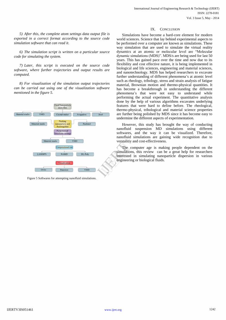
5) After this, the complete atom settings data output file is
exported in a correct format according to the source code
simulation software that can read it.
6) The simulation script is written on a particular source
code for simulating the system.
7) Later, this script is executed on the source code
software, where further trajectories and output results are
computed.
8) For visualization of the simulation output trajectories
can be carried out using one of the visualization software
mentioned in the figure 5.
Figure 5 Softwares for attempting nanofluid simulations.
IX. CONCLUSION
Simulations have become a hard-core element for modern world sciences. Science that lay behind experimental aspects to be performed over a computer are known as simulations. These way simulation that are used to simulate the virtual reality dynamics at an atomic or molecular level are ―Molecular dynamic simulations (MDS)‖. MDS/s are being used for last 50 years. This has gained pace over the time and now due to its flexibility and cost effective nature, it is being implemented in biological and life sciences, engineering and material sciences, and nanotechnology. MDS has helped researchers to excavate further understanding of different phenomena‘s at atomic level such as rheology, tribology, stress and strain analysis of fatigue material, Brownian motion and thermo-physical quantities. It has become a breakthrough in understanding the different phenomena‘s that were not easy to understand while performing the actual experiment. The quantitative analysis done by the help of various algorithms excavates underlying features that were hard to define before. The rheological, thermo-physical, tribological and material science properties are further being polished by MDS since it has become easy to undermine the different aspects of experimentation.
However, this study has brought the way of conducting nanofluid suspension MD simulations using different softwares, and the way it can be visualized. Therefore, nanofluid simulations are gaining wide recognition due to verstalitiy and cost-effectiveness.
The computer age is making people dependent on the simulations, this review can be a great help for researchers interested in simulating nanoparticle dispersion in various engineering or biological fluids.
1242
International Journal of Engineering Research & Technology (IJERT)
IJERT
IJERT
ISSN: 2278-0181
www.ijert.orgIJERTV3IS051461
Vol. 3 Issue 5, May - 2014

Table 1. Force field classical energy function.
Equations Energy
calculation
methods
Graphical illustration Variable resemblance
2
0
1( )
2r
bonds
k r r Bond stretches
2
0
1( )
2angles
k Angle bending
0,1 cos[ ( )]2
ni i i
torsions
Vn
Torsional
rotation
i j
elec ij
q q
r
Electrostatic
interaction
12 6
0, 0,
,
[ 2 ]ij ij
ij ij
Pairs ij ij ij
r r
r r
Van der Waal-
interaction
Table 2. Nanofluid simulations historical background and applications for different systems.
S No. Simulation On What Forcefield/
potentials used
Year Properties
Analysed
1 Adil Loya et al.
[33]
CuO in water COMPASS
forcefield, DPD
potential and SPH potential
2014 Viscosity and
diffusion properties
2 Ali Rajab pour et al. [44]
Cu water simulation L-J potential and Lorentz-Berthlot
2013 Specific heat capacity
3 Hongbo et al. [45]
Cu-Ar Ar-Ar L-J Potential 2012 Diffusion
4 Ali Mohebbi [46]
Beta-Si3N4 in argon system
L-J Potential, Morse function and
Charm FF
2012 Thermal conductivity and
specific heat
5 Yung Sheng Lin et EthyleneGlycol-Cu L-J Potential, 2012 Thermal
1243
International Journal of Engineering Research & Technology (IJERT)
IJERT
IJERT
ISSN: 2278-0181
www.ijert.orgIJERTV3IS051461
Vol. 3 Issue 5, May - 2014

al.
[1]
Morse potential,
Lorrentz Berthelot
mixing rule and JR
FF
conductivity
6 Wenzheng Cui
[47]
Cu in argon liquid L-J Potential 2011 Turbulance model
7 Valery Ya Rudyak
et al. [48]
General Np in dense
fluid
L-Jpotential and R-
K Potential
2011 Coupling factor
8 Chengzhen Sun et al.
[37]
Cu-Ar nanofluid L-J Potential and EAM potential
2011 Thermal conductivity
9 D.L Cheung
[49]
Nanopartilce-solvent L-J potential 2010 Diffusion and RDF
10 N.Sankar et al.
[50]
Pt-water and pt-pt L-J potential, Morse
potential and FENE
potential
2008 Thermal
conductivity
11 Wen-Qiang Lu et al.
[51]
Alumina-water or
C2H5OH or C2H4(OH)2
L-J potential 2008 Thermal
conductivity and viscosity
12 Ling Li et al. [52]
Cu-Ar L-J potential 2008 Thermal conductivity
13 S. Sarkar et al. [53]
Cu-Ar EAM and L-J Potential
2007 Thermal conductivity and
Diffusion
14 Mingxiang Luo et
al.
[54]
Hydrocarbon-water-
polymer Np
Gromos force field
and L-J potential
2006 Density and
diffusion
15 Delphine Barbier et al.
[55]
PEO Oilogomers melts with silica
nanoparticles
L-J potential, UFF and OPLS FF
2004 Density and RDF
16 Francis W. Starr et
al.
[56]
Polymer melt with np L-J potential and
FENE model
2002 Density and RDF
17 Anatoly Malevanets
et al. [57]
Nanocolloidal model L-J potential 2000 Velocity
Autocorrelation Function (VACF),
Diffusion
18 D M Heyes et al.
[58]
Colloidal model WCA and L-J
potential
1998 RDF, VACF,
Density and
diffusion
Table 3. Nanofluid simulation dispersion properties equations used in most molecular dynamics calculations.
1244
International Journal of Engineering Research & Technology (IJERT)
IJERT
IJERT
ISSN: 2278-0181
www.ijert.orgIJERTV3IS051461
Vol. 3 Issue 5, May - 2014

REFERENCES
[1] Y.-S. Lin, P.-Y. Hsiao, C.-C. Chieng, Thermophysical characteristics
of ethylene glycol-based copper nanofluids using nonequilibrium and
equilibrium methods, International Journal of Thermal Sciences, 62 (2012) 56-60.
[2] C.W. Sohn, M.M. Chen, Microconvective thermal conductivity in
disperse two-phase mixtures as observed in a low velocity couette flow experiment, Journal Name: J. Heat Transfer; (United States);
Journal Volume: 103:1, (1981) Medium: X; Size: Pages: 47-51.
[3] J. Chevalier, O. Tillement, F. Ayela, Rheological properties of nanofluids flowing through microchannels, Applied Physics Letters,
91 (2007) 233103-233103-233103.
[4] D.W. Litchfield, D.G. Baird, The rheology of high aspect ratio nano-particle filled liquids, Rheology Reviews, 2006 (2006) 1.
[5] P.K. Namburu, D.P. Kulkarni, A. Dandekar, D.K. Das, Experimental
investigation of viscosity and specific heat of silicon dioxide nanofluids, Micro & Nano Letters, IET, 2 (2007) 67-71.
[6] S.M. Hosseini, E. Ghasemi, A. Fazlali, D. Henneke, The effect of
nanoparticle concentration on the rheological properties of paraffin-based Co3O4 ferrofluids, J Nanopart Res, 14 (2012) 1-7.
[7] A. Aqil, H. Serwas, J.L. Delplancke, R. Jérôme, C. Jérôme, L. Canet, Preparation of stable suspensions of gold nanoparticles in water by
sonoelectrochemistry, Ultrasonics Sonochemistry, 15 (2008) 1055-
1061. [8] D.J. Cooke, J.A. Elliott, Atomistic simulations of calcite nanoparticles
and their interaction with water, The Journal of Chemical Physics,
127 (2007) 104706-104709. [9] B. Streszewski, W. Jaworski, K. Pacławski, E. Csapó, I. Dékány, K.
Fitzner, Gold nanoparticles formation in the aqueous system of
gold(III) chloride complex ions and hydrazine sulfate—Kinetic studies, Colloids and Surfaces A: Physicochemical and Engineering
Aspects, 397 (2012) 63-72.
[10] D.A. Giljohann, D.S. Seferos, W.L. Daniel, M.D. Massich, P.C.
Patel, C.A. Mirkin, Gold Nanoparticles for Biology and Medicine,
Angewandte Chemie International Edition, 49 (2010) 3280-3294.
[11] R.S.K. Shriram S. Sonawane, Kailas L. Wasewar and Ajit P. Rathod Dispersions of CuO Nanoparticles in Paraffin Prepared by
Ultrasonication: A Potential Coolant 3rd International Conference on
Biology, Environment and Chemistry, IPCBEE vol.46 (2012) © (2012)IACSIT Press, Singapore (2012).
[12] S. Pandey, M. Thakur, R. Shah, G. Oza, A. Mewada, M. Sharon, A
comparative study of economical separation and aggregation properties of biologically capped and thiol functionalized gold
nanoparticles: Selecting the eco-friendly trojan horses for biological
applications, Colloids and surfaces. B, Biointerfaces, 109 (2013) 25-31.
[13] S.U. Choi, J. Eastman, Enhancing thermal conductivity of fluids with
nanoparticles, in, Argonne National Lab., IL (United States), 1995. [14] S. Lee, S.-S. Choi, S. Li, and, J. Eastman, Measuring thermal
conductivity of fluids containing oxide nanoparticles, Journal of Heat
Transfer, 121 (1999) 280-289.
[15] F. Duan, D. Kwek, A. Crivoi, Viscosity affected by nanoparticle
aggregation in Al2O3-water nanofluids, Nanoscale Research Letters,
6 (2011) 248. [16] C.T. Nguyen, F. Desgranges, G. Roy, N. Galanis, T. Maré, S.
Boucher, H. Angue Mintsa, Temperature and particle-size dependent
viscosity data for water-based nanofluids – Hysteresis phenomenon, International Journal of Heat and Fluid Flow, 28 (2007) 1492-1506.
[17] C. Zhao, Y.K. Chen, G. Ren, A Study of Tribological Properties of
Water-Based Ceria Nanofluids, Tribology Transactions, 56 (2013) 275-283.
[18] C. Zhao, Y.K. Chen, Y. Jiao, A. Loya, G.G. Ren, The preparation
and tribological properties of surface modified zinc borate ultrafine powder as a lubricant additive in liquid paraffin, Tribology
International, 70 (2014) 155-164.
[19] C. Zhao, Y. Chen, G. Ren, A study of tribological properties of water-based ceria nanofluids, Tribology Transactions, 56 (2013) 275-
283.
[20] M.J. Pastoriza-Gallego, C. Casanova, J.L. Legido, M.M. Piñeiro, CuO in water nanofluid: Influence of particle size and polydispersity
on volumetric behaviour and viscosity, Fluid Phase Equilibria, 300 (2011) 188-196.
[21] A. Hernández Battez, R. González, J.L. Viesca, J.E. Fernández, J.M.
Díaz Fernández, A. Machado, R. Chou, J. Riba, CuO, ZrO2 and ZnO nanoparticles as antiwear additive in oil lubricants, Wear, 265 (2008)
422-428.
[22] M.-O. Coppens, A.T. Bell, A.K. Chakraborty, Effect of topology and molecular occupancy on self-diffusion in lattice models of zeolites—
Monte-Carlo simulations, Chemical Engineering Science, 53 (1998)
2053-2061. [23] M. Levitt, M. Hirshberg, R. Sharon, V. Daggett, Potential energy
function and parameters for simulations of the molecular dynamics of
proteins and nucleic acids in solution, Computer Physics
Communications, 91 (1995) 215-231.
[24] J.R. Spaeth, I.G. Kevrekidis, A.Z. Panagiotopoulos, A comparison of
implicit- and explicit-solvent simulations of self-assembly in block copolymer and solute systems, The Journal of Chemical Physics, 134
(2011) 164902-164913.
[25] J.M. Haile, Molecular Dynamics Simulation: Elementary Methods, Wiley, 1997.
[26] S.M. Langenegger, R. Haner, Excimer formation by interstrand
stacked pyrenes, Chemical Communications, (2004) 2792-2793. [27] S. Patel, C.L. Brooks, CHARMM fluctuating charge force field for
proteins: I parameterization and application to bulk organic liquid
simulations, Journal of Computational Chemistry, 25 (2004) 1-16. [28] K.H. Lee, F.M. Ytreberg, Effect of gold nanoparticle conjugation on
peptide dynamics and structure, Entropy, 14 (2012) 630-641.
[29] H. Sun, P. Ren, J.R. Fried, The COMPASS force field: parameterization and validation for phosphazenes, Computational and
Theoretical Polymer Science, 8 (1998) 229-246.
Property Definition Statisical Mechanical
formula
Einstein Relation for larger t
Diffusion
Coefficient
nn D
x
0
1. 0
3i iv t v dt
21
06
i ir t rt
Thermal
conductivity T
qx
2
0
. 0B
Vq t q dt
K T
2
20
2B
Vt
K T t
Shear Viscosity UF
x
2
( )( )
4
dn rg r
r dr
0
. 0B
Vp t p dt
K T
( )( ) exp
B
u rg r
K T
2
02B
VD t D
K T t
None
RDF
1245
International Journal of Engineering Research & Technology (IJERT)
IJERT
IJERT
ISSN: 2278-0181
www.ijert.orgIJERTV3IS051461
Vol. 3 Issue 5, May - 2014

[30] H. Sun, COMPASS: An ab Initio Force-Field Optimized for
Condensed-Phase ApplicationsOverview with Details on Alkane and Benzene Compounds, The Journal of Physical Chemistry B, 102
(1998) 7338-7364.
[31] S.W. Bunte, H. Sun, Molecular Modeling of Energetic Materials: The Parameterization and Validation of Nitrate Esters in the
COMPASS Force Field, The Journal of Physical Chemistry B, 104
(2000) 2477-2489. [32] J.D. Kubicki, Molecular mechanics and quantum mechanical
modeling of hexane soot structure and interactions with pyrene,
Geochemical Transactions, 1 (2000) 1-6. [33] A. Loya, S. J.L., R. G., The Study Of Simulating Metaloxide
Nanoparticles In Aqueous Fluid. , International Journal of
Engineering Research & Technology, 3 (2014) 1954-1960. [34] B. Prathab, V. Subramanian, T. Aminabhavi, Molecular dynamics
simulations to investigate polymer–polymer and polymer–metal oxide
interactions, Polymer, 48 (2007) 409-416. [35] R.V. Pappu, R.K. Hart, J.W. Ponder, Analysis and Application of
Potential Energy Smoothing and Search Methods for Global
Optimization, The Journal of Physical Chemistry B, 102 (1998) 9725-
9742.
[36] W.R. Scott, P.H. Hünenberger, I.G. Tironi, A.E. Mark, S.R. Billeter,
J. Fennen, A.E. Torda, T. Huber, P. Krüger, W.F. van Gunsteren, The GROMOS biomolecular simulation program package, The Journal of
Physical Chemistry A, 103 (1999) 3596-3607.
[37] C. Sun, W.-Q. Lu, J. Liu, B. Bai, Molecular dynamics simulation of nanofluid‘s effective thermal conductivity in high-shear-rate Couette
flow, International Journal of Heat and Mass Transfer, 54 (2011) 2560-2567.
[38] D.L.M. Ermak, J. A., Brownian dynamics with hydrodynamic
interactions, J. Chem. Phys., 69 (1978) 1352-1360. [39] R.A. Gingold and J.J. Monaghan, ―Smoothed particle
hydrodynamics: theory and application to non-spherical stars,‖ Mon.
Not. R. Astron. Soc, Vol 181, pp. 375–89 (1977). [40] J.J. Monaghan, Smoothed particle hydrodynamics, Reports on
Progress in Physics, 68 (2005) 1703.
[41] G.C. Ganzenmuller, a.M.O. Steinhauser, The implementation of Smooth Particle Hydrodynamics in
LAMMPS., (2011).
[42] P.J.H.a.J.M.V.A. Koelman, Simulating microscopic hydrodynamic phenomena with dissipative particle dynamics,
Europhys.Lett.,19:155-160, (1992).
[43] P. Español, P. Warren, Statistical Mechanics of Dissipative Particle Dynamics, EPL (Europhysics Letters), 30 (1995) 191.
[44] A. Rajabpour, F. Akizi, M. Heyhat, K. Gordiz, Molecular dynamics
simulation of the specific heat capacity of water-Cu nanofluids, International Nano Letters, 3 (2013) 58.
[45] H. Kang, Y. Zhang, M. Yang, L. Li, Nonequilibrium molecular
dynamics simulation of coupling between nanoparticles and base-fluid in a nanofluid, Physics Letters A, 376 (2012) 521-524.
[46] A. Mohebbi, Prediction of specific heat and thermal conductivity of
nanofluids by a combined equilibrium and non-equilibrium molecular dynamics simulation, Journal of Molecular Liquids, 175 (2012) 51-
58.
[47] J. Lv, M. Bai, W. Cui, X. Li, The molecular dynamic simulation on impact and friction characters of nanofluids with many nanoparticles
system, Nanoscale Research Letters, 6 (2011) 1-8.
[48] V. Rudyak, S. Krasnolutskii, D. Ivanov, Molecular dynamics simulation of nanoparticle diffusion in dense fluids, Microfluid
Nanofluid, 11 (2011) 501-506.
[49] D.L. Cheung, Molecular simulation of nanoparticle diffusion at fluid interfaces, Chemical Physics Letters, 495 (2010) 55-59.
[50] N. Sankar, N. Mathew, C.B. Sobhan, Molecular dynamics modeling
of thermal conductivity enhancement in metal nanoparticle suspensions, International Communications in Heat and Mass
Transfer, 35 (2008) 867-872.
[51] W.-Q. Lu, Q.-M. Fan, Study for the particle's scale effect on some
thermophysical properties of nanofluids by a simplified molecular
dynamics method, Engineering Analysis with Boundary Elements, 32
(2008) 282-289. [52] L. Li, Y. Zhang, H. Ma, M. Yang, An investigation of molecular
layering at the liquid-solid interface in nanofluids by molecular
dynamics simulation, Physics Letters A, 372 (2008) 4541-4544. [53] S. Sarkar, R.P. Selvam, Molecular dynamics simulation of effective
thermal conductivity and study of enhanced thermal transport mechanism in nanofluids, Journal of Applied Physics, 102 (2007) -.
[54] M. Luo, O.A. Mazyar, Q. Zhu, M.W. Vaughn, W.L. Hase, L.L. Dai,
Molecular Dynamics Simulation of Nanoparticle Self-Assembly at a Liquid−Liquid Interface, Langmuir, 22 (2006) 6385-6390.
[55] D. Barbier, D. Brown, A.-C. Grillet, S. Neyertz, Interface between
End-Functionalized PEO Oligomers and a Silica Nanoparticle Studied by Molecular Dynamics Simulations, Macromolecules, 37
(2004) 4695-4710.
[56] F.W. Starr, T.B. Schrøder, S.C. Glotzer, Molecular Dynamics Simulation of a Polymer Melt with a Nanoscopic Particle,
Macromolecules, 35 (2002) 4481-4492.
[57] A. Malevanets, R. Kapral, Solute molecular dynamics in a mesoscale solvent, The Journal of Chemical Physics, 112 (2000) 7260-7269.
[58] D.M. Heyes, M.J. Nuevo, J.J. Morales, A.C. Branka, Translational
and rotational diffusion of model nanocolloidal dispersions studied by molecular dynamics simulations, Journal of Physics: Condensed
Matter, 10 (1998) 10159.
Abbreviation Table and their units
Symbols Meanings CuO Copper Oxide
CuO-NP/s Copper OxideNanoparticle/s
DLVO Derjaguin and Landau, Verwey and Overbeek
EAM/MEAM Embedded Atom Method/Modified Embedded Atom
Method
LJ Lenord Jones
NVE Number of atoms, Volume and Energy
NVT Number of atoms, Volume and Temperature
NPT Number of atoms, Pressure and Temperature
UFF Universal Forcefield
AMBER Assisted Model Building Energy Refinement
CHARMM Chemistry At Harvard Macromolecular Mechanics
COMPASS Condensed-phase Optimized Molecular Potential for
Atomistic Simulation studies
OPLS Optimized Potentials for Liquid Simulations
DPD Discrete particle dynamics
MD Molecular dynamics
BD Brownian Dynamics
1246
International Journal of Engineering Research & Technology (IJERT)
IJERT
IJERT
ISSN: 2278-0181
www.ijert.orgIJERTV3IS051461
Vol. 3 Issue 5, May - 2014
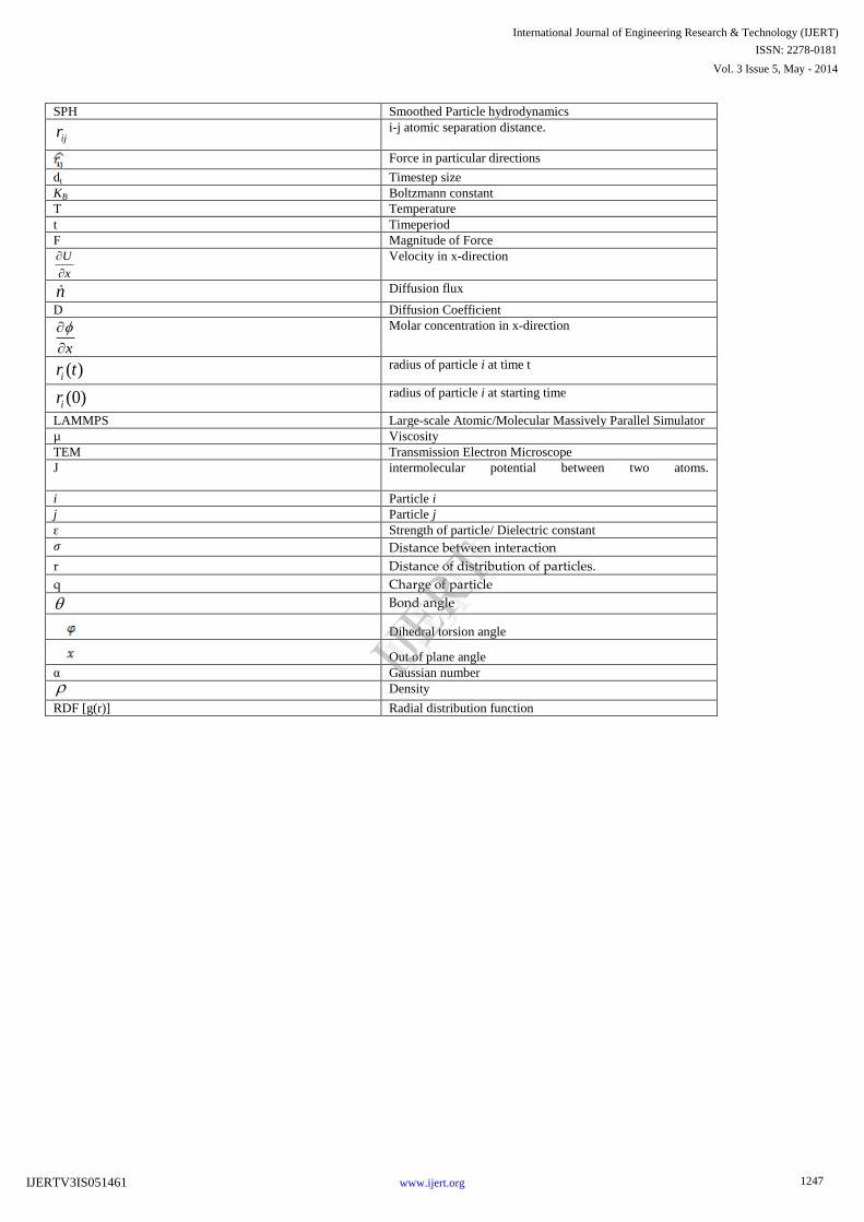
SPH Smoothed Particle hydrodynamics
ijr i-j atomic separation distance.
Force in particular directions
dt Timestep size
KB Boltzmann constant
T Temperature
t Timeperiod
F Magnitude of Force
U
x
Velocity in x-direction
n Diffusion flux
D Diffusion Coefficient
x
Molar concentration in x-direction
( )ir t radius of particle i at time t
(0)ir radius of particle i at starting time
LAMMPS Large-scale Atomic/Molecular Massively Parallel Simulator
µ Viscosity
TEM Transmission Electron Microscope
J intermolecular potential between two atoms.
i Particle i
j Particle j
ԑ Strength of particle/ Dielectric constant
𝜎 Distance between interaction
r Distance of distribution of particles.
q Charge of particle
Bond angle
Dihedral torsion angle
Out of plane angle
α Gaussian number
Density
RDF [g(r)] Radial distribution function
1247
International Journal of Engineering Research & Technology (IJERT)
IJERT
IJERT
ISSN: 2278-0181
www.ijert.orgIJERTV3IS051461
Vol. 3 Issue 5, May - 2014