THE APPLICATION OF CFD TO BUILDING … · Specification of the modeling context: scope and resources.37 ... specification of data and other prior knowledge.....37 4.2.4. Selection

THE APPLICATION OF CFD TO BUILDING ANALYSIS AND DESIGN:

A COMBINED APPROACH OF AN IMMERSIVE CASE STUDY AND

WIND TUNNEL TESTING

Daeung Kim

Dissertation submitted to the Faculty of the Virginia Polytechnic Institute and State University in

partial fulfillment of the requirements for the degree of

Doctor of Philosophy

in

Architecture and Design Research

James R. Jones, Chair

Robert P. Schubert

Elizabeth J. Grant

Demetri P. Telionis

Saad A. Ragab

December 11, 2013

Blacksburg, Virginia

Keywords: Computational Fluid Dynamics, building design, design assistance tool, immersive

case study, wind tunnel tests

Copyright 2013, Daeung Kim

THE APPLICATION OF CFD TO BUILDING ANALYSIS AND DESIGN:

A COMBINED APPROACH OF AN IMMERSIVE CASE STUDY AND

WIND TUNNEL TESTING

Daeung Kim

ABSTRACT

Computational Fluid Dynamics (CFD) can play an important role in building design. For all

aspects and stages of building design, CFD can be used to provide more accurate and rapid

predictions of building performance with regard to air flow, pressure, temperature, and similar

parameters.

Generally, the process involved in conducting CFD analyses is relatively complex and requires a

good understanding of how best to utilize computational numerical methods. Moreover, the level

of skill required to perform an accurate CFD analysis remains a challenge for many professionals

particularly architects. In addition, the user needs to input a number of different items of

information and parameters into the CFD program in order to obtain a successful and credible

solution.

This research seeks to improve the general understanding of how CFD can best be used as a

design assistance tool. While there have been a number of quantitative studies suggesting CFD

may be a useful tool for building related airflow assessment, few researchers have explored the

more qualitative aspects of CFD, in particular developing a better understanding of the

procedures required for the proper application of CFD to whole building analysis. This study

therefore adopted a combined qualitative and quantitative methodology, with the researcher

immersing himself into a case study approach and defining several lessons-learned that are

documented and shared. This research will assist practicing architects and architecture students

to better understand the application of CFD to building analysis and design.

DEDICATION

In my memory, my father didn�t say much, but I could feel your love.

While I am finishing this journey, I miss you the most and I won�t forget your smile at the airport

when I left for the United States.

Without your support and encouragement, I couldn�t get to the end of this journey.

With my full respect, I dedicate this dissertation to you, my father,

Chun-Hwan Kim (1949 � 2010).

I also dedicated my dissertation to my family in South Korea:

My dear mom, for her greatest sacrifices and praying;

My lovely wife, Gajin Moon and our first baby, for care, support and patience;

My sister, Boram Kim, for her support;

Parents-in-law, for their support and encouragement

I love you all.

ACKNOWLEDGEMENTS

I would like to thank my supervisor, Dr. James R. Jones, for his guidance, assistance,

encouragement, and patience. During my journey, his insightful guidance showed me the way to

go forward. In addition, his way of conducting research made me to realize what the researcher�s

role is between Architecture and Engineering. Without his advice and support, I couldn�t

complete this journey. Thank you, Jim. Your thoughtful guidance always reminds me of the

famous quotes from the movie �Dead Poets Society�. That is �Oh Captain, My Captain.�

I would also like to thank the members of my committee. Thank you, Dr. Elizabeth Grant, for

your insightful ideas. Thank you, Prof. Robert Schubert, for your support and advice. Thank you,

Dr. Saad Ragab, for your advice in conducting CFD simulation and kindness. Thank you, Dr.

Demetri Telionis.

I am also thankful to CD-adapco, Computer-aided engineering company, for providing the

academic license for the CFD simulation package �STAR-CCM+� without a charge.

Many thanks to my colleagues, Naif Altahlawi, Kongkun Charoenvisal, Bandar Alkahlan,

Mohammed Aloshan, Vidya Gowda and Ana Jaramillo, for their warm words and support.

A special thanks to Heejin Jung, who is one of my best friends in Blacksburg, for his support and

wishes.

TABLE OF CONTENTS

TABLE OF CONTENTS��..

LIST OF FIGURES��...xxi

LIST OF EQUATIONS��.xxix

LIST OF TABLES��.��xxx

1. INTRODUCTION��....1

1.1. Background��.1

1.2. Wind tunnel tests��...��..2

1.3. CFD simulations for building design��..3

1.4. General use of CFD as a design assistance tool��.6

1.5. Problem statement��..8

1.6. Scope of research��9

1.6.1. Primary goal ��.9

1.6.2. Research objectives��...9

1.7. Significance��....10

1.8. Limitations��.10

1.9. Dissertation outlines��...11

2. QUALITATIVE RESEARCH APPROACH��.13

2.1. Qualitative research method��...13

2.2. Utilizing the case study approach ��..15

2.3. Overview of case study approach��...16

2.4. Case study research design��.16

2.5. Selection of the cases��..18

2.6. Objectives of the case study��...19

2.7. Data collection��21

2.8. Analysis of case study evidence��.22

2.9. Validity of the study��...22

2.10. Research�s role��..23

3. BEST PRACTICE GUIDELINES FOR CFD��..24

3.1. Overview of best practice guidelines��.24

3.2. Recommendations for the use of CFD for wind around buildings��25

3.2.1. Geometrical representation ��.26

3.2.2. The computational domain ��..27

3.2.3. Computational grid��...28

3.2.4. Boundary conditions��.....30

3.2.5. Turbulence models��32

3.2.6. Convergence criteria��.32

3.3. Summary of the best practice guidelines��....33

4. THE TEN ITERATIVE STEPS APPROACH��.��.35

4.1. Introduction��....35

4.2. The characteristics of the ten iterative steps approach��...35

4.2.1. Definition of the purposes for modeling��...36

4.2.2. Specification of the modeling context: scope and resources��.�37

4.2.3. Conceptualization of the system, specification of data and other prior

knowledge��.��....37

4.2.4. Selection of model features and families��..37

4.2.5. Choice of how model structure and parameter values are to be found�....37

4.2.6. Choice of estimation performance criteria and technique��....38

4.2.7. Identification of model structure and parameters��.38

4.2.8. Conditional verification including diagnostic checking��...38

4.2.9. Quantification of uncertainty��39

4.2.10. Model evaluation or testing (other models, algorithms, comparisons

with alternatives)��.......39

4.3. Selection of journals��....40

4.4. Lessons-learned from the journal one: Numerical simulation of dispersion

around an isolated cubic building: Model evaluation of RANS and LES

(Tominaga & Stathopoulos, 2010)��........41


4.4.2. Specification of the modeling context: scope and resources��....42

4.2.2.1. Available resources��.............42

4.4.2.2. Forcing variables and required outputs��..42

4.4.2.3. Spatial and temporal scope, scale and resolution��...43

4.4.2.4. Users of the model and model flexibility��...44


knowledge��.....44

4.4.4. Selection of model features and families��....45

4.4.5. Choice of how model structure and parameter values are found��...45

4.4.6. Choice of performance criteria��...........46

4.4.7. Identification of model structure and parameters��...........47

4.4.8. Conditional verification including diagnostic checking��.47

4.4.9. Quantification of uncertainty��......48

4.4.10.Model evaluation or testing (other models, algorithms, comparisons with

alternatives) ��.��...48

4.5. Lessons-learned from the journal two: wind-induced pressure coefficients

on buildings with and without balconies (Montazeri & Blocken, 2013)��..51

4.5.1. Definition of the purposes for modeling��...........51


4.5.2.1. Available resources��...........51

4.5.2.2. Forcing variables and required outputs��52

4.5.2.3. Spatial and temporal scope, scale and resolution��.53

4.5.2.4. Users of the model and model flexibility��.55


knowledge��56


4.5.5. Choice of how model structure and parameter values are found��.57

4.5.6. Choice of performance criteria��.57





with alternatives) ��.59

4.6. Lessons-learned from the journal three: Effect of roof shape, wind direction,

building height and urban configuration on the energy yield and positioning

of roof mounted wind turbines (Abohela et al., 2013)��61


4.6.2. Specification of the modeling context: scope and resources��.61

4.6.2.1. Available resources��....61

4.6.2.2. Forcing variables and required outputs��.62

4.6.2.3. Spatial and temporal scope, scale and resolution��..63

4.6.2.4. Users of the model and model flexibility��...64


knowledge��.64


4.6.4.1. Modeling approach��65

4.6.4.2. Conceptual model��.65







with alternatives) ��.67

4.7. Lessons-learned from the journal four: Near-field pollutant dispersion in

the built environment by CFD and wind tunnel simulations (Chavez et al.,

2011)��.��...��69

4.7.1. Definition of the purposes for modeling��...........69


4.7.2.1. Available resources��....70

4.7.2.2. Forcing variables and required outputs��.71

4.7.2.3. Spatial and temporal scope, scale and resolution��..72

4.7.2.4. Users of the model and model flexibility��..73


knowledge��.....74


4.7.4.1. Modeling approach��74

4.7.4.2. Conceptual model��.75

4.7.4.3. Spatial and temporal scales��...75



4.7.7. Identification of model structure and parameters��.....76



4.7.10. Model evaluation or testing (other models, algorithms, comparisons with

alternatives) ��..77

4.8. Summary of lessons-learned from the journal analysis��.��79

5. WIND TUNNEL TESTING��.83

5.1. Architectural applications of wind tunnel testing��.�.83

5.2. Overview of wind tunnel testing at IBHS��.....83

5.2.1. The IBHS wind facility��.84

5.2.2. Facility details of the IBHS��..86

5.3. Experimental configuration��.��..87

5.4. Results��...........92

6. THE SENSITIVITY ANALYSIS��.94

6.1. Introduction ��...94

6.2. Context of the wind tunnel tests at the IBHS��.�94

6.3. Other computational parameters��.�....95

6.4. Investigations of wind flow on a roof with three different computational domain

sizes��.....�95

6.4.1. Problem statement��..�95

6.4.2. Computational domain��.�..96

6.4.3. Computational grid��.�....97

6.4.4. Boundary conditions��.�.99

6.4.5. Other computational conditions��...100

6.4.6. CFD simulation results��.100

6.4.6.1. Qualitative comparisons��100

6.4.6.2. Comparisons of pressure coefficient on the roof surface of three

models��105

6.4.7. Discussion��.106

6.5. The sensitivity analysis of impact of the computational grid resolution��108

6.5.1. Problem statement��108

6.5.2. Computational domain��.108


6.5.4. Boundary conditions��.109

6.5.5. Other computational conditions��.�...111

6.5.6. CFD simulation results��.111



grids. ..��..115

6.5.7. Discussion��.��...116

6.6. The sensitivity analysis of impact of turbulence model��.��116

6.6.1. Case study problem statement��..116

6.6.2. The Selection of turbulence models��.117



6.6.5. Other computational parameters��...118

6.6.5.1. Parameters for LES��...��119

6.6.6. Other computational conditions��.��...119

6.6.7. CFD Simulation Results��...120



turbulence models��..124

6.6.8. Discussion��.125

6.7. Summary of the sensitivity analysis��..��..125

6.8. Computational parameters for wind flow around building through research

process��.126

7. IMMERSIVE CASE STUDY��...�...128

7.1. Introduction ��...��..128

7.2. Preparation for input computational parameters ��...��..129

7.2.1. The selection of the turbulence model ��...��.��..129

7.2.2. The selection of the geometry ��...��..�..130

7.2.3. Other computational parameters ��.................��..131

7.3. Case study A: An investigation of wind flow over a flat roof for two different

building heights��...��...132

7.3.1. Introduction and context��.��132

7.3.2. Computational domain��132

7.3.3. Computational grid��.134

7.3.4. Boundary conditions��...135

7.3.5. Other computational parameters��.�135

7.3.6. CFD simulation results��....�...136

7.3.6.1 Qualitative comparisons��..136

7.3.6.2. Comparisons of pressure coefficient distributions on the roof

surfaces��....137

7.3.7. Discussion��...138

7.4. Case Study B: A comparisons of wind flow over a flat roof surface with two

different building aspect ratios��...�139

7.4.1. Introduction and context��139

7.4.2. Computational domain��...�140

7.4.3. Computational grid��.141


7.4.5. Other computational parameters��.�143

7.4.6. CFD simulation results��....143



surfaces��....145

7.4.7. Discussion��...146

7.5. Case Study C: A comparisons of wind flow over the flat roof surface of a low-

rise building with three different parapet walls��..�147

7.5.1. Introduction and context��.�147

7.5.2. Computational domain��...�.�147

7.5.3. Computational grid��...��..148


7.5.5. Other computational parameters��.149

7.5.6. CFD simulation results��150



surfaces��.�..151

7.5.7. Discussion��..152

7.6. Summary of case studies��..�..153

7.7. Discussion of the computational parameters through case studies��154

8. CFD AS A DESIGN ASSITANCE TOOL IN SCHEMATIC DESIGN STAGE��...155

8.1. Selecting the commercial code��....�155

8.2. Preparing the geometry ��..�.156

8.3. The computational domain size ��..�158

8.4. Grid generation��162

8.5. Turbulence model��..��..�163

8.6. Boundary conditions��165

8.7. Numerical schemes and the algorithm ��166

8.8. Convergence criterion ��.166

8.9. Conclusions regarding the CFD simulation process for wind comfort around

buildings in the schematic design stage ��...167

8.9.1. Pre-processing��.�167

8.9.2. Solving��168

8.9.3. Post-processing��...168

9. LESSONS-LEARNED��.�170

9.1. Introduction��..170

9.2. Consider influential factors in the urban area including vegetation and

surface characteristics when preparing the geometry��.170

9.3. Clean up and reproduce the initial design of the building of interest and

surroundings in the native AutoCAD file as much as possible before importing

them into the computational domain��...171

9.4. Choose the proper grid type for various applications of building design��171

9.5. Consider the smallest length scale of the building of interest when determining

the base size of grids and check for computational errors after grid

generation��.��..��.�173

9.6. Choose the proper turbulence model for applications of building design, namely

either LES or the RANS turbulence model��.....�174

9.7. Use the default values provided for turbulence quantities in the commercial

code for the inlet boundary condition when experimental data is not

available��...��..�..175

9.8. Monitor the residuals and visualization of the results while calculating the

solutions��..��176

9.9. Practice an effective visualization of the results��..��178

10. CONCLUSIONS��..��.�180

10.1. Introduction��.��.�.180

10.2. Methodology��...��...181

10.3. Research findings��.�..182

10.3.1. Selecting the commercial code��. ��182

10.3.2 Preparing the geometry��.��.............182

10.3.3. Importing the geometry��...��..183

10.3.4. Creating the computational domain��.��.183

10.3.5. Generating grids��..�..183

10.3.6.Selecting turbulence model��..��..184


10.3.8. Numerical schemes and the algorithm��..185

10.3.9. Convergence criterion��...�186

10.4. Recommendations for the computational parameters for various building

design objectives��.186

10.5. Lessons-learned through the research process��...188

10.6. Suggestions for further research��189

REFERENCES��..��..193

APPENDICES��..��...209

Appendix A: CFD procedures��....��........209

Appendix B: CFD fundamentals��...��.........210

1. Governing equations��.210

2. Initial conditions��...211

3. Grid generation��.211

4. Discretization��212

5. Turbulence models��214

6. Solution algorithm��.216

7. Boundary conditions��.217

8. Numerical parameters for controlling the calculation ��..217

Appendix C: Definitions of several CFD terms��..��...�218

Appendix D: The commercial CFD codes��.��..��..221

1. FLUENT��...........221

2. STAR-CCM+��222

3. The selection of CFD code��....223

LIST OF FIGURES

Figure 1.1 Various CFD applications for building design: a. Assessment of pedestrian

wind comfort (Janssen et al., 2013), b. Prediction of natural ventilation

(Bangalee et al., 2012), c.Investigation of HVAC system for indoor

environment (Chiang et al., 2012), and d. Prediction of pollutant

dispersion (Gousseau et al., 2011)��...6

Figure 1.2 Architectural design process with CFD simulation��.7

Figure 2.1 Overview of the case study design��..20

Figure 3.1 An example of geometric resolution (Blocken et al., 2012): a. Aerial

view of the geometry for CFD resolution and b. Corresponding

high-resolution computational grid��..27

Figure 3.2 Dimensions of the domain grid (Lateb et al., 2013)��28

Figure 4.1 Iterative relationship between model building steps. (Jakeman et al., 2006)�..36

Figure 4.2 Computational domain and boundary conditions of LES

(Tominaga & Stathopoulos, 2010)��...43

Figure 4.3 Distribution of time-averaged dimensionless concentration (K) on roof

and wall surfaces (Tominaga & Stathopoulos, 2010): (1) RNG, (2)

LES and (3) Exp��...49

Figure 4.4 Distribution of time-averaged dimensionless concentration (K) on the

centerline of the roof and leeward and side walls (Tominaga &

Stathopoulos, 2010): (1) Streamwise direction and (2) Lateral direction��50

Figure 4.5 Geometry of building model and balconies (unit:mm) (Montazeri &

Blocken, 2013)��.53

Figure 4.6 Computational grid (Montazeri & Blocken, 2013): a. Grid at bottom

and side faces of computational domain, b. Grid at building surfaces

and ground surface and c. Detail of grid near balconies��..54

Figure 4.7 Computational grids for grid-sensitivity analysis (Montazeri & Blocken,

2013): a. Coarse grid, b. Basic grid and c. Fine grid��...55

Figure 4.8 The results of pressure coefficient distribution and velocity vector

field (Montazeri & Blocken, 2013): a. Pressure coefficient across

windward façade of building with balconies, b.Velocity vector

field in cross-section of building with balconies, c. Pressure

coefficient across windward façade of building without balconies

and d.Velocity vector field in cross-section of building without

balconies��..��60

Figure 4.9 Results for grid-sensitivity analysis with three different grids (Montazeri

& Blocken, 2013): a. Pressure Coefficient along edge line and

Pressure coefficient along center line��..��60

Figure 4.10 Roof shapes, from top left: flat, domed, gabled, pyramidal, barrel vaulted

and wedged (Abohela et al., 2013)��.�.62

Figure 4.11 The results of straemwise velocity pathlines and the pressure

distribution (Abohela et al., 2013): a. Stremwise velocity pathlines

through the vertical central plan and b. Streamwise velocity pathlines

at ground level��.63

Figure 4.12 Mesh refinement areas around the cube (Abohela et al., 2013)��..64

Figure 4.13 Optimum mounting location for different investigated roof shapes under

0 wind direction (Abohela et al., 2013): flat, domed, gabled, pyramidal,

barrel vaulted and wedged (from top left)��68

Figure 4.14 The results of streamlines velocity pathlines for the 12 and 24 m vaulted

building (Abohela et al., 2013): a. Streamlines velocity pathlines along

the central vertical axis for the 12 m vaulted building and b. Streamlines

velocity pathlines along the central vertical axis for the 24 m

vaulted building��.��..68

Figure 4.15 Three cases for CFD simulation (Chavez et al., 2011)��.�...70

Figure 4.16 Plan view and elevation (Chavez et al., 2011)��.�....71

Figure 4.17 Boundary conditions used for the CFD model (Chavez et al., 2011)��..72

Figure 4.18 Perspective view of the mesh of isolated building case B1

(Chavez et al., 2011)��73

Figure 4.19 Contours of mean velocity magnitude (m/s) for stack height h - 1 m and

exhaust momentum M � 3 (Chavez et al., 2011): a. case 1, b. case 2 and

c. case 3��78

Figure 5.1 IBHS Research Center in Richburg, SC (Morrison et al., 2012a):

a. Aerial photograph of the IBHS Research Center and

b. 105 fans of the Inlet��.85

Figure 5.2 Plan view and elevation views of the IBHS facility (Liu et al., 2009)��85

Figure 5.3 Wind vanes at the inlet of the IBHS wind facility��.......86

Figure 5.4 Layout of the IBHS Research Center test chamber and inlet from

the fans (Morrison et al., 2012a)��..87

Figure 5.5 The overall view of the wind tunnel facility: a. Test building and

b. Layout of the test building and the chamber��88

Figure 5.6 The location of the pressure taps on the roof of the test building��....90

Figure 5.7 Mean velocity (left) and longitudinal turbulence intensity (Iu)

(right) profiles (Morrison et al., 2012a)��...91

Figure 5.8 Pressure coefficient distribution on the roof surface (Morrison et al., 2012b)�92

Figure 5.9 Pressure coefficient distribution along the centerline on the roof surface��...93

Figure 6.1 Three different computational domains: a. Computational domains for

the reference model, b. Computational domains for the model with 2H of

the upstream length and c.Computational domains for the increased

blockage ratio model��98

Figure 6.2 The inlet boundary conditions: a. The mean wind speed profile by

power law and b. Turbulence kinetic energy k��...�.........100

Figure 6.3. Contours and vectors of mean velocity magnitude for the middle vertical

plan: a. The reference model, b. 2H of upstream length and

c. The increased blockage ratio��102

Figure 6.4 Contours of mean velocity magnitude on the roof surface: a. The reference

model, b. 2H of upstream length and c. The increased blockage ratio��103

Figure 6.5 Contours of pressure coefficients distribution on the roof surface: a. The

reference model, b. 2H of upstream length and c. The increased

blockage ratio��...104

Figure 6.6 Comparison of pressure coefficient from CFD simulation results and

wind tunnel measurements along the roof surface centerline��..105

Figure 6.7 Impact of the computational domain size on CFD simulation results

for the pressure coefficient along the roof surface centerline��..�106

Figure 6.8 Comparison of pressure coefficients along the centerline of the windward

façade, roof and leeward façade with the average of the 15 wind tunnel tests,

the Silsoe 6 m cube full scale measurement and CFD simulation

(Abohela et al., 2013)��...107

Figure 6.9 Three different computational grids for grid-sensitivity analysis The

reference model: 682,380 cells The coarse grids: 98,510 cells

The fine grids: 1,590,548 cells��.110

Figure 6.10 Contours and vectors of mean velocity magnitude for the middle vertical

plan: a. The reference model: 682,380 cells, b. The coarse grids: 98,510 cells

and c. The fine grids: 1,590,548 cells��..112


model, b. The coarse grids and c. The fine grids��..113


reference model, b. The coarse grids and c. The fine grids��.�.114

Figure 6.13 Results of the grid sensitivity analysis: pressure coefficient along the

centerline of the roof surface��.��...115

Figure 6.14 Contours and vectors of mean velocity magnitude for the middle vertical

plan: a. The reference model: the Realizable k-ɛ turbulence model,

b. The Standard k-ɛ turbulence model and c. The LES model…………………121


model: the Realizable k-ɛ turbulence model, b. The Standard k-ɛ turbulence

model and c. The LES model…………………………………………………...122


reference model: the Realizable k-ɛ turbulence model, b. The

Standard k-ɛ turbulence model and c. The LES model…………………….…..123

Figure 6.17 CFD simulation results: Impact of turbulence models on the pressure

coefficients along the centerline of the roof surface……………………………124

Figure 7.1 Prototype of the roof vent system (Grant, 2003, p. 35)..……………………….128

Figure 7.2 The result of contours and vectors of the mean velocity magnitude for the

middle vertical plane of a building when the RANS turbulence model was

applied………………………………………………………………………….130

Figure 7.3 The result of contours and vectors of the mean velocity magnitude for the

middle vertical plane of a building with the roof surface area 150,000 ft2….....131

Figure 7.4 Two different building height : a. Reference model: Height=36 ft and

b.Building with height=12 ft…………………………………………………...132

Figure 7.5 The two different computational domains: a. Reference model (building

height: 36 ft) and b. The 12 ft high building…………………………………....133

Figure 7.6 The computational grids: a. Computational grids for the reference model

and b. Computational grids for the 12 ft high building……………………........134

Figure 7.7 Contours and vectors of mean velocity magnitude on the roof and for the

middle vertical plane: a. The reference model and b. The 12 ft high building…136

Figure 7.8 Contours of pressure coefficients on the roof : a. The reference model and

b. The 12 ft high building ……………………...................................................137

Figure 7.9 CFD simulation results for the pressure coefficient along the centerline of

the roof surface for the two structures………………………………………….138

Figure 7.10 Two different building aspect ratios Reference model: a. Aspect ratio 1:2

and b. Test building: aspect ratio 1:1…………………………………………...140

Figure 7.11 Two different computational domain: a. Reference model with the building

aspect ratio 1:2 and b. Test building with the building aspect ratio 1:1………...141

Figure 7.12 The computational grids: a. Computational grids for the reference model

with a building aspect ratio 1:2 and b. Computational grids for the building

with a building aspect ratio 1:1………………………………………………....142

Figure 7.13 Contours and vectors of mean velocity magnitude on the roof and for the

middle vertical plane: a. The reference model: Aspect ratio 1:2 and

b. The building with aspect ratio 1:1……………………………………………144

Figure 7.14 Contours of pressure coefficients on the roof: a. The reference model and

b. Test building with a height of 12ft ……………………………………….….145

Figure 7.15 Results of pressure coefficients along the centerline of the roof surface……….146

Figure 7.16 The reference building with three different parapet walls: 3 in, 24 in

and 42 in (From the top)………………………………………………………..147

Figure 7.17 The computational domain for the reference model…………………………...148

Figure 7.18 The computational grids for the three different parapet walls:

a. Computational grids for the reference building with the 3 in curb edge,

b. Computational grids for the reference building with 24 in parapet

wall and c. Computational grids for the building with 42 in parapet wall……...149

Figure 7.19 Contours and vectors of mean velocity magnitude on the roof and for

the middle vertical plane: a. The reference model with the parapet wall

height 42 in, b. The building with the parapet wall height 24 in and

c. The building with the curb edge……………………………………………..150

Figure 7.20 Contours of pressure coefficient on the roof: a. The reference model

with the parapet wall height 42 in, b. The building with the parapet wall

height 24 in and c. The building with the curb edge……………………………151

Figure 7.21 CFD simulation results: Impact of turbulence models on the pressure

coefficients along the centerline of the roof surface……………………………152

Figure 8.1 Aerial view of the area north of the Amsterdam ArenA football stadium

and its surroundings (Hooff & Blocken, 2010)…………………………………157

Figure 8.2 Grid generation for the Amsterdam ArenA football stadium and surroundings

: (a) Computational model geometry, view from northeast; (b) computational

grid for the building surfaces and part of the ground surface (Hooff &

Blocken, 2010)………………………………………………………………….157

Figure 8.3 Standard wind rose with frequency distribution of the hourly mean wind

speed for Eindhoven University campus (Janssen et al., 2013)………………...158

Figure 8.4 A single building in the computational domain: a. Test building in the wind

tunnel at the IBHS, b. Layout of the test building and the chamber and

c. The test building in the computational domain……………………………...160

Figure 8.5 The computational domain of an urban area in Antwerp (Montazeri et al.

2013): a. Aerial view of the Park Tower (red) and surrounding buildings,

b. Top view of Park Tower and wider surroundings in a rectangular area

of 630–1000 m2 with an indication of building heights and

c. Computational domain for wind directions 180°–270°, consisting of

a basic domain and an additional downstream domain…………………………161

Figure 9.1 An example of the residuals during calculation of the sensitivity

analysis in Chapter 6..……………………………………….….……….….…..177

Figure 9.2 Monitoring the vector and contour plots of mean velocity during calculation

of the sensitivity analysis in Chapter 6...…………………………….………....177

Figure 9.3 An example of the visualization of CFD results…………………………….….179

APPENDICES

Figure 1 The two different mesh types (Bosbach et al.,2006): a. Unstructured

mesh and b. Structured mesh…………………………………………………...212

Figure 2 Close-up view of a hybrid computational grid (Zhang & Wang, 2004)………..212

Figure 3 Structured meshes for the two main discretization methods

(Molina-Aiz et al., 2010): a. FEM and b. FVM………………………………...214

LIST OF EQUATIONS

Equation 5.1 Calculation of the pressure coefficient………………………………………..89

Equation 6.1 Calculation of the turbulence kinetic energy……………….………………....99

Equation 6.2 Calculation of the turbulence dissipation rate…………………….…………..99

Equation 8.1 A log-law for the wind profile ………………………………………………..165

Equation 8.2 A power law for the mean velocity profile .…………………………………..165

APPENDICES

Equation 1 The conservation of mass……………………………………………………..210

Equation 2 A momentum equation………………………………………………………..210

LIST OF TABLES

Table 2.1 Overview of the three case projects……………………………………………..19

Table 4.1 Selected journal papers…………………………………………………….…....40

Table 4.2 Comparison of reattachment lengths on roof and behind cube (Tominaga

& Stathopoulos, 2010)…………………………………………………………..48

Table 4.3 Building models for CFD and wind tunnel experiments (Chavez et

al., 2011)………………………………………………………………………...70

Table 4.4 A summary of lessons-learned: the computational parameters for

wind flow around buildings………..……………………………………………82

Table 6.1 A summary of computational parameters for wind flow around building

through research process………………………………………………………..127

Table 8.1 Comparison between the characteristics of FLUENT and STAR-CCM+……...156

Table 8.2 Comparison between the characteristics of hexahedral and tetrahedral grids….162

Table 8.3 Comparison of the characteristics of the RANS approach and

the LES model………………………………………………………………….164

Table 8.4 Values for typical terrain dependent parameters in the UK (Cook, 1997,

as quoted in Drew et al., 2013)…………………………………………………166

Table 9.1 Recommendations for the selection of a suitable grid type for

various applications……………………………………………………………..173

Table 9.2 Recommendations for the selection of turbulence model for

various applications……………………………………………………………..175

Table 10.1 Recommendations for the computational parameters for various building

design objectives………………………………………………………………..187

APPENDICES

Table 1 File formats for importing into FLUENT (ANSYS FLUENT, 12.0

User’s Guide)…………………………………………………………………...222

Table 2 File formats for importing into STAR-CCM+ (STAR-CCM+ user

guide 8.04)……………………………………………………………………...223

1. INTRODUCTION

1.1. Background

Natural disasters such as cyclones, earthquakes, floods and landslides strike various parts of the

world every year. In the United States alone, these cause hundreds of deaths and cost billions of

dollars in disaster aid annually. According to the preliminary report issued by NOAA’s National

Climatic Data Center (Graumann et al., 2005), Hurricane Katrina has been the most expensive

natural disaster in recent U.S. history. Although only a Category 3 hurricane, Katrina caused

massive devastation along the central Gulf Coast states of the U.S. and was responsible for more

than 1,800 deaths.

Wind fluctuations during high wind events can have a serious effect on building envelopes, often

with serious consequences such as roof failures (Morrison & Kopp, 2011) because wind uplift

pressure makes roof membranes flutter or rapidly flap up and down (Baskaran et al., 2009).

According to Blessing et al. (2009), the resulting loss of roofing leads to rainwater intrusion,

interior restoration and occupant displacement. Moreover, roofing elements separated by high

winds become wind-borne debris that then cause further damage to other structures downwind.

Suaris and Irwin (2010) found that the uplift pressure generated by corner vortices can create

very high intermittent suction. Aerodynamic loads on the roof and walls of a low building are

characterized by the interaction of wind flow with the surface of the building and this interaction

depends primarily on the building geometry and flow characteristics (Stathopoulos, 1984).

However, architects and engineers seldom consider these issues but instead tend to focus

primarily on design and structural aspects related to elements such as walls, overhangs,

foundation and roofing when designing buildings.

Managing the risk to buildings from wind requires detailed information on the type and

magnitude of the wind loads that buildings are likely to be exposed to. Recent attempts to

minimize damage due to high winds have been devoted to developing more reliable estimates of

wind effects on buildings. For example, Tieleman et al. (1998) used a 1:50 scale model of the

WERFL experimental building in the wind load test facility at Clemson University to examine

how the pressure coefficient varied with horizontal turbulence intensity, the small-scale

turbulence parameter and the streamwise and lateral turbulence integral scale. Chen and Zhou

(2007) investigated the equivalent static wind loads on low-rise buildings based on full-scale

measurements, while wind-induced torsional loads on low rise buildings were reported by

Elsharawy et al. (2012), who assessed the effectiveness of three national building codes and

standards, namely ASCE 7 (United States), NBCC (Canada), and EN 1991-14 (Australia). Ho et

al. (2005) studied the effect of the surroundings on wind loads on flat roof low buildings,

examining several cases of similar buildings with different types of immediate surroundings.

Traditionally, this information has been gathered using a combination of wind tunnel tests and

full-scale measurements. However, these field studies can be both time-consuming and costly so

Computational Fluid Dynamics (CFD) methods are becoming more widely accepted as an

alternative tool for predicting turbulent flow over buildings and thus informing their design. CFD

methods are convenient to access for design practice and can simulate the flow field about a

building and predict parameters of interest such as velocity, pressure, and temperature fields

(Alexander et al., 1997). CFD techniques are now commonly applied in a number of industries.

1.2. Wind tunnel tests

Wind tunnels have been employed extensively for both industry and research applications over

the past 50 years. Varying greatly in scale and geometry, some facilities are large enough to

house and test small aircraft while others are miniaturized to accommodate the flow generators

used in the calibration of small sensors (Morrison & Kopp, 2011). Wind tunnels are used to study

the flow of air over objects of interest, the forces acting on them, and their interaction with the

flow and have been employed to verify aerodynamic theories and facilitate the design of aircraft,

as well as to develop new aircraft, wind turbines and other designs that involve complex

interactions with an airflow (Hernandez et al., 2013).

On Mar 23 – 24, 2012, wind tunnel testing was conducted at the IBHS in Richburg, SC to

investigate the performance of roof vent systems developed by Virginia Tech and Acrylife Inc.

For this study, the data from these wind tunnel tests were utilized to validate the results of the

CFD modeling.

1.3. CFD simulations for building design

Due to the time and cost issues involved in wind tunnel testing, CFD is now widely employed for

the prediction of flow fields. The first CFD techniques were introduced in the early 1950s, made

possible by the advent of the digital computer (Chung, 2002). CFD is a computer-based

mathematical modeling tool capable of dealing with fluid flow problems and predicting physical

fluid flows and heat transfer (Versteeg & Malalasekera, 1995). While traditionally thought of as

exclusively for use in aerodynamic research, CFD analysis is now being applied in many other

fields, including marine engineering, electrical and electronic engineering, biomedical

engineering, chemical engineering, environmental engineering, wind engineering, hydrology,

oceanography, meteorology, and nuclear power (Versteeg & Malalasekera, 1995). As the range of

CFD applications continues to increase, new techniques have been introduced that facilitate its

use in both architectural engineering and HVAC (heating ventilating and air conditioning) design

(Zhang et al., 2009). It is particularly useful for building design and analyses, where it has been

applied with considerable success (Murakami, 1998). There are now numerous commercial CFD

software packages that are targeted specifically toward building applications.

CFD is used intensively as a tool for evaluating the indoor environment of a building and its

interaction with the building envelope, as well as for analyzing the outdoor environment

surrounding the building (Blocken et al., 2009). For the prediction of external wind flows, CFD

can be used to analyze wind loading on buildings, bridges, and street canyons. For example,

Sengupta et al. (2008) simulated the effects of microburst and tornadic winds to quantify the

resulting aerodynamic loading on a building in order to investigate the peak loads and stresses at

various locations on a roof and then compared the results to the corresponding values for the

guidelines specified in ASCE 7-05. In a study examining pedestrian wind comfort, Janssen et al.

(2013) compared and evaluated various wind comfort criteria to highlight the importance of

standardizing the wind comfort assessment procedure using CFD techniques. For their research

on predicting pollutant dispersion, Gousseau et al. (2011) employed CFD to investigate pollutant

concentrations in streets and on building surfaces surrounding the source. CFD has also been

applied to test proposed natural ventilation, mixed-mode ventilation, and HVAC systems in

buildings (Hooff & Blocken, 2012; Balocco & Lio, 2011; Bangalee et al., 2012; Chiang et al.,

2012), which generally involves the prediction of air temperature, velocity, and relative humidity,

among other parameters. CFD techniques have been used to simulate the spread of fire and

smoke through large-volume spaces (Huang et al., 2009) as well as being applied in clean rooms

and buildings in order to protect against biochemical and radioactive agents and provide

contamination control (Rui et al., 2008). Figure 1.1 shows several examples of CFD applications

that enhance building performance.

According to Wainwright and Mulligan (2004), CFD offers a number of advantages compared to

traditional wind tunnel testing. Not only can CFD generate full-scale simulations as opposed to

scale models of many physical simulations, it also provides more extensive data than can be

measured in the lab and its results can be visualized clearly and in great detail. On the other hand,

CFD also has several drawbacks and issues. Knowledge and experience of fluid mechanics are

required to evaluate CFD results critically and a good understanding of how a CFD code

functions for a particular application is essential if the results are to be meaningful. In addition,

the cost of purchasing a commercial CFD package is high and a high-performance computer is

required.

a. Assessment of pedestrian wind comfort (Janssen et al., 2013)

b. Prediction of natural ventilation (Bangalee et al., 2012)

c. Investigation of HVAC system for indoor environment (Chiang et al., 2012)

d. Prediction of pollutant dispersion (Gousseau et al., 2011)

Figure 1.1 - Various CFD applications for building design

1.4. General use of CFD as a design assistance tool

According to the AIA (American Institute of Architects), design and construction projects

typically involve several phases (The five phases of design, the AIA).

In the first stage, the most important decisions are made. In this stage, discussions regarding the

project requirements are conducted, with stakeholders presenting their expectations for aspects

such as the number of rooms, functions and occupants to the design team. These discussions

enable the scope of the design project to be outlined. Once the object to be built has been defined,

the next step is to create schematic designs. During the schematic design stage, study drawings,

documents, or other media that illustrate the concepts of the design and include spatial

relationships, scale, and form for the owner to review are developed. The third step is design

development. In this phase, the initial designs from the second phase are developed further by

adding details of the project’s mechanical, electrical, plumbing, and structural elements, and

architectural documents are provided. After the design development phase is complete,

construction documents are prepared. Once the construction documents are finalized, the general

contractor or builder who will undertake the actual construction is hired (The five phases of

design, the AIA).

During the schematic phase, CFD is often employed to calculate airflows in and around the

buildings. Based on the calculated results, it typically determines whether the design needs to be

modified. In order to achieve satisfactory indoor and outdoor environmental conditions for the

building, these steps will be repeated iteratively as often as necessary to achieve a satisfactory

result (Glicksman, & Lin, 2006).

As indicated above, CFD techniques are now commonly used as a design assistance tool. The

results from CFD simulations during the schematic design stage can help architects or designers

to improve the indoor and outdoor environment for the planned building at the schematic design

stage. Figure 1.2 shows the architectural design process when CFD simulation is used.

This study demonstrates the use of the CFD process as a design assistance tool for building

design and provides recommendations to ensure the effective use of CFD simulation results.

Figure 1.2 - Architectural design process with CFD simulation

1.5. Problem statement

The demand for new, easier to use CFD applications continues to increase and many commercial

CFD codes are now available that are designed to be used by non-CFD experts. Many architects

have begun to take advantage of CFD techniques as a design assistance tool because CFD

analyses can provide detailed information throughout all stages of the design process, providing

a flexible and interactive design environment for design decision making. However, there are

several potential pitfalls that users need to constantly bear in mind. First, CFD is difficult to use

in the architectural design process because of its relatively complicated process and time

consuming aspects such as the generation of complex geometries. Second, various calculation

conditions, such as the size of the computational domain, grid resolution, boundary conditions,

selection of the turbulence model, and so on must be set by the user. As Ferziger (1990) pointed

out, the selection of boundary conditions is not a simple matter in the numerical solution of

turbulent flow. Third, although many CFD publications on building performance have focused

on the quantitative aspects of the problem, far fewer have reported qualitative investigations into

the effectiveness of adopting CFD as a design assistance tool. Instead, most numerical studies

have conducted straightforward quantitative comparisons of model predictions against

experimental observations.

Understanding the CFD process and its limitations is crucial if it is to become a dependable tool

for design and analyses. By considering the challenges described above and how they relate to

the needs of architects, the findings of this study will assist designers. Although some

preliminary quantitative procedures are used, the main focus of this study is on the qualitative

aspects of the problem in order to bridge the gap between architecture and engineering.

1.6. Scope of research

1.6.1. Primary goal

This research seeks to improve our understanding of how best to utilize CFD as a design

assistance tool for architecture. While a number of quantitative studies have suggested that CFD

may be a useful tool for building related airflow assessment (Ramponi & Blocken, 2012; Lo et

al., 2013; Hooff & Blocken, 2013), there have been few studies exploring the more qualitative

aspects of CFD, including the development of suitable procedures for the proper application of

CFD to whole building analysis. Adopting a combined qualitative and quantitative investigation,

in the course of which the researcher immersed himself in the case study approach for analyzing

wind effects on building roofs, enabled him to develop a set of lessons-learned that can be

documented and shared. This research thus applied a combined method using both qualitative

and quantitative techniques to maximize the effective use of CFD as a design assistance tool and

to minimize any inaccuracies related to its application for building design in the schematic

design stage.

1.6.2. Research objectives

A thorough literature review and journal analysis of the key computational parameters and

conditions involved in CFD analyses of wind flow around buildings was conducted for this study.

These selected parameters were examined and validated utilizing the data gathered during wind

tunnel tests conducted at the IBHS. Results of a sensitivity analysis comparing CFD to wind

tunnel data were then used to inform the immersive case study. The observations were gathered

and discussed in the context of the themes that emerged from the data during the case studies.

Throughout this process, lessons-learned were documented. The outcome was a rich description

of the simulation process and a summary of lessons-learned to inform the practice of those using

CFD for building airflow analysis.

1.7. Significance

The significance and unique contribution of this research is that it considered the challenges of

CFD simulation from a designer’s point of view. Its findings include a comprehensive set of

recommendations to guide the use of CFD for the prediction of building performance that are

expected to provide a greatly improved understanding of how to apply CFD methods to best

effect during the building design process.

1.8. Limitations

In order to predict air flow in and around a building, CFD analyzes the air velocity, temperature,

contaminant concentrations, and amount of turbulence around that building by solving a set of

mathematical equations. It is therefore necessary to conduct mathematical modeling at the outset

to establish the necessary computational inputs. Unlike other building simulations such as energy

simulations, CFD requires users to have some knowledge of mathematical modeling and

experience with numerical methods. In addition, the CFD modeling approach relies on physical

models such as turbulence. However, computational domains for outdoor environment studies

can be very large and the boundary conditions are not always well-known (Blocken et al., 2011).

This may lead to very large computational errors in the simulation results. It is difficult for non-

experts or architects to conduct CFD simulations.

Moreover, this research employed a qualitative approach using case study methods. For this

approach, the primary instrument of data collection and analysis is the researcher. However, it is

difficult for case study researchers to act as trained observers. In addition, the research outcome

is generally heavily dependent on the researcher’s own instincts and abilities.

In this research, the critical computational inputs were established through case study methods.

As a building designer, it is not always easy to completely understand mathematical equations

and physical models in real world. The computational inputs utilized were those established by

previous researchers and reported in the literature, particularly the findings of studies

investigating wind flow in building applications using CFD techniques. Less rigorous

commercial CFD codes are available that can be used in building practice and for analyses of the

built environment. These commercial codes include advanced techniques that automate much of

the data specification process for common situations. Moreover, the limitations of case study

methods can be overcome by employing iterative methods such as the document analysis and an

immersive approach.

1.9. Dissertation outline

Chapter Two presented the qualitative research approach to provide an in-depth description of

the CFD process as a design assistance tool. A review of the qualitative research method and the

case study approach was presented in this chapter. For this approach, the research design, data

collection, case study evidence and the validity were presented in detail.

In order to choose the initial computational parameters for CFD simulation at the early design

stage, best practice guidelines were briefly reviewed in Chapter Three and a set of computational

parameters for wind flows around buildings reviewed. However these selected parameters were

not sufficient to ensure credibility, and therefore the ten-steps approach was employed. The

characteristics of this approach were summarized in Chapter Four. In this chapter, four journal

articles related to the application of CFD for wind flows around buildings were analyzed using

the ten-steps approach in order to obtain specific computational parameters.

Computational results should be validated with experimental data whenever possible to ensure

their credibility and reliability. For this validation and to inform the CFD simulation process,

wind tunnel testing was conducted at the IBHS wind facility. An overview of these wind tunnel

tests and their results were presented in Chapter Five.

Using the computational parameters from Chapters Three and Four, three sensitivity analyses

were conducted and these were presented in Chapter Six. CFD simulations were compared with

the wind tunnel testing at the IBHS as described in Chapter Five. These results included the

velocity and pressures along the centerline and on the roof of the building.

The computational parameters selected in Chapters Three to Six were employed in the case study.

The wind flow behaviors on the roof surface of a low-rise building with several building

configurations, including various building heights, aspect ratios and parapet wall heights were

investigated in Chapter Seven. For the case study, some computational parameters were

subsequently reselected based on these results.

The computational parameters from Chapters Six and Seven were analyzed and are categorized

under two themes in Chapter Eight. Discussions of the CFD process for wind flow around

buildings considering the accuracy and the effective use of CFD in the schematic design stage

were presented in this chapter.

Chapter Nine was devoted to a set of the lessons-learned from the present study. In Chapter Ten,

the conclusions and some recommendations were made for future research.

2. QUALITATIVE RESEARCH APPROACH

The main goal of this research is to provide an in-depth description of the CFD process in order

to improve our understanding of its use as a design assistance tool. This chapter outlines the

rationale supporting the utility of qualitative research methods and the case study approach and

describes the case study research design and methods used for this study. Multiple case study

methods are explored and the case selection process, methods of data collection and analysis of

the collected data are described.

2.1. Qualitative research method

This research makes use of qualitative research methodologies to understand the process of

applying CFD tools to issues related to building design as a decision-support tool following the

recommendations provided by Linda Groat and David Wang. In their book Architectural

Research Methods, Groat and Wang address the �generic� definition of qualitative research

originally stated by Norman Denzin and Yvonne Lincoln as follows:

Qualitative research is multi-method in focus, involving an interpretive, naturalistic approach

to its subject matter. This means that qualitative researchers study things in their natural

settings, attempting to make sense of, or interpret, phenomenon in terms of the meanings

people bring to them. Qualitative research involves the studied use and collection of a variety

of empirical materials (Denzin & Lincoln, 1998, as quoted in Groat & Wang, 2002, p. 176).

This definition implies that the value of the research is precisely due to its ability to highlight

trends embedded in the context of the academic departments the subjects are a part of. They

ground their work in the empirical realities of their observations and interviews, while at the

same time making it clear that they, as researchers, play an important role in interpreting and

making sense of that data. Researchers aim to present a holistic portrayal of the setting or

phenomenon under study as the respondents themselves understand it. Groat and Wang also

pointed out that the strategy of qualitative research consists of first-hand encounters with a

specific context and thus involves gaining an understanding of how people in real-world

situations �make sense� of their environment and themselves using a variety of tactics. They

provide the following summary of the attributes of qualitative research design, based on previous

researchers� descriptions:

Holistic. The goal of qualitative research is to gain a holistic (systematic, encompassing,

integrated) overview of the context under study.

Prolonged Contact. Qualitative research is conducted through an intense and/or prolonged

contact with a �field� or life situation.

Open Ended. Qualitative research tends to be more open-ended in both theoretical conception

and research design than other research strategies.

Researcher as Measurement Device. Since there is relatively little use of standardized measures

such as survey questionnaires, the researcher is essentially the main measurement device in the

study.

Analysis Through Words. Since an emphasis on descriptive numerical measures and inferential

statistics is typically eschewed, the principal mode of analysis is through words, whether

represented in visual displays or through narrative devices.

Personal Informal Writing Stance. In contrast to the typical journal format of experimental or

correlational studies, the writing style of qualitative work is typically offered in a personal

informal writing stance that lessens the distance between the writer and the reader (Groat &Wang,

2002, p. 179).

This description goes a long way towards describing the aims and strategies of the present

research. Here, the actions will be those components of the lessons related to the CFD simulation

that most accurately reflect the reality and the understanding of its application. Groat and Wang

(2002) conclude that the major strengths of qualitative research follow from its capacity to take

in the rich qualitative information available in real-life circumstances and settings. Based on this

qualitative research method, a direct means of achieving this is as a participant observer directly

involved in the prediction of building design and systems in order to answer the research

question concerning the applicability of the CFD technique. In addition to the information

gleaned as a participant observer and through direct observation of a CFD case study for building

design and systems, information that addresses the research question will be gathered through the

researcher�s practice as an architect. It is through this practice that a participant observer can gain

a more comprehensive understanding of what lessons can be learned about the utility of CFD as

a decision-support technique.

2.2. Utilizing the case study approach

This qualitative study is concerned with improving our understanding of CFD as a technique for

studying airflow around buildings. In order to perform this study, a case study approach was

adopted. According to Rowley (2002), case studies as a research method or strategy have

traditionally been considered as lacking rigor and objectivity comparing with other social

research methods. However, in spite of this skepticism they are widely accepted by researchers

in many fields since they can offer insights that might not be achieved with other approaches.

Rowley (2002) also mentioned that case studies have often been considered a useful tool for the

preliminary, exploratory stage of a research project in order to provide a basis for the

development of the �more structured� tools that are necessary in surveys and experiments. Robert

Yin quotes a useful definition of case studies given by an earlier researcher in his book Case

Study Research (1994):

The essence of a case study, the central tendency among all types of case study, is that it tries

to illuminate a decision or set of decisions: why they were taken, how they were implemented,

and with what result (Schramm, 1971, quoted in Yin, 1994, p.17).

He explores the concept further to provide an alternative definition:

A case study is an empirical inquiry that investigates a contemporary phenomenon within its

real-life context, especially when the boundaries between phenomenon and context are not

clearly evident (Yin, 1994, p.18).

Yin (1994) emphasized that an important strength of case studies is their ability to facilitate an

investigation into a phenomenon in its context. Thus, the replication of the phenomenon in a

laboratory or experimental setting is no longer necessary to achieve a better understanding of the

phenomena, making the case study method a valuable way of looking at the world around us.

Moreover, case study research can be based on any mix of quantitative and qualitative

approaches and can utilize multiple data sources, including direct/participant observations,

interviews, and documents (Rowley, 2002).

The goal of this study has been to improve our understanding of the use of CFD as an

architectural design tool. Many researchers have shown that CFD studies can provide useful

information, demonstrating good statistical and quantitative reliability between experiments and

simulations (Ramponi & Blocken, 2012; Hooff & Blocken, 2012; Chavez et al, 2011; Blocken et

al, 2008), and the increasing use of CFD has led to it being applied for a wide range of purposes

in built environments. However, real-world projects may involve conditions or parameters that

are either unfamiliar or too complex to apply to different situations. To determine the limits that

should be applied to restrict the scope of its use, the applicability of CFD will be studied in the

context of wind flow over a roof by adopting a case study strategy.

2.3. Overview of case study approach

The case study performed for this research was designed to obtain a holistic description of the

CFD modeling process in the context of wind flow around a building. The following sections

will discuss, in turn, the guidelines for data collection, analysis, and the decision-making process

regarding which evidence to pursue and information to collect among the available data.

2.4. Case study research design

The design of a case study encompasses the logic that connects the data to be collected and the

conclusions to be drawn to the initial questions addressed by the study. This ensures that there is

a clear view of what is to be achieved by the case study. This process includes defining the basic

components of the investigation, such as the research questions and propositions, determining

how validity and reliability will be established, and selecting an appropriate case study design

(Rowley, 2002).

Among these components, the research question is perhaps the most significant element in

determining the most appropriate research approach. Who, what and where questions can be

investigated through documents, archival analysis, surveys and interviews (Yin, 1994). As

mentioned previously, this study is based on the CFD modeling process. However, issues

concerning the credibility and acceptance of CFD results remain due to its complexity and the

number of computational parameters. Thus, the research questions guiding this case study are:

1) What computational parameters are used in the context of the CFD analysis of wind flow

around a building?

2) How has the wind tunnel testing informed the CFD modeling process?

3) How are the credibility and reliability of the CFD results determined?

4) What CFD tool is most appropriate to support architectural design decision making? and

5) How can CFD modeling be integrated with the architectural design process?

According to Yin (1994), the design of a case study can be classified along two dimensions,

reflecting the number of case studies contributing to the design, and the number of units in each

case study, respectively. It is important to make a distinction between single case and multiple

case designs. A single case design is appropriate when the case is closely linked to an established

theory for some reason. This might occur when the case provides a critical test of a well-

established theory, for example, or where the case is extreme, unique, or has something special to

reveal. In the case of a multiple case design, the more cases that can be included to establish or

refute a theory, the more robust the resulting research outcomes. In a multiple case design cases

should be chosen carefully in order to produce either similar or contrasting results.

For this study, a multiple case design was employed. Each case was investigated using a

conceptual framework to include as wide a range as possible of contextual factors and outcomes

to be explored and compared. The context of interest for the case studies focused on the wind

flow around a building. Multiple sources of evidence, including documents, participant

observation, archival records and artifacts, were collected to ensure the strength of the case study

methodology.

2.5. Selection of the cases

After taking the decision to adopt a multiple case study design for this study, the next issue was

the number of cases that should be included in the research project. Cases are typically selected

purposively to maximize learning about the research questions, in contrast to the quantitative

ideal of a random sample that is statistically representative of a larger population (Patton, 2002;

Yin, 1994). With regard to the sample size, Patton argued that �There are no rules for sample size

in qualitative inquiry. Sample size depends on what you want to know, the purpose of the inquiry,

what�s at stake, what will be useful, what will have credibility, and what can be done with the

available time and resources� (2002, p. 244). Yin (1994) suggested that the decision on sample

size should reflect the number of replications of both literal and theoretical aspects of the

problem and that this replication is one of the most powerful ways to ensure the high credibility

of the results. In order to identify patterns of similarity, the sample size will be determined based

on the literal replication.

Another important consideration in selecting the cases to be included in a multiple case design is

the specific sampling strategy utilized (Patton, 2002). Patton suggested that �Because research

and evaluations often serve multiple purposes, more than one qualitative sampling strategy may

be necessary . . . The sampling strategy must be selected to fit the purpose of the study, the

resources available, the questions being asked, and the constraints being faced� (2002, p. 242).�

In order to achieve a better understanding of the problem and the research questions, cases were

therefore selected purposefully for this case study (Cresswell, 2009). Three cases were selected

and each case conducted a CFD simulation in order to examine wind flow on the roof surface

with several building configurations including the building height, aspect ratio and parapet wall

heights. The three cases are presented in Table 2.1.

Table 2.1- Overview of the three case projects

Cases Projects

Case A An investigation of wind flow on a roof with two different building heights

Case B A comparisons of wind flow on the roof surface with two different building aspect ratios

Case C A comparisons of wind flow on the roof surface of a low-rise building with three different parapet walls

2.6. Objectives of the case study

In order to address the study�s overarching research questions, a set of substantive research

objectives was developed to achieve a robust, holistic description of the CFD simulation for the

investigation of wind flow around buildings in the architectural design process. Figure 2.1

showed an overview of the major components of the case study design. In this figure, the

objectives provided a roadmap for data collection and analysis, guiding decisions on what

documentary evidence to pursue and what information to gather through participant observation

during two design stages. The objectives are:

1) Early design stage

- In order to reproduce wind flow around buildings using CFD, computational parameters were

selected through document analysis and the sensitivity tests.

- Best practice guidelines were reviewed to select computational parameter for wind flow around

buildings (Chapter 3).

- Four journal articles were analyzed in order to achieve specific computational parameters for

wind flow around buildings (Chapter 4).

- The sensitivity of selected computational parameters from best practice guidelines and the

analysis of journal articles were analyzed using the data of wind tunnel tests at the IBHS

(Chapter 5 & 6).

- The chosen computational parameters through Chapter 4 to 7 were applied and analyzed

through case studies (Chapter 7).

2) Schematic design stage

- The computational parameters of the early stage were categorized and analyzed under two

categories (Chapter 8):

a) What are the computational parameters to maximize the accuracy of the CFD

modeling? and,

b) What are the computational parameters for the effective use of CFD as a design

assistance tool regarding time consuming aspects and easy use of CFD?

- Through research process, lessons-learned to inform CFD process for building design were

documented (Chapter 9).

Figure 2.1 - Overview of the case study design

2.7. Data collection

Typically, case studies draw on multiple sources of evidence including documents, archival

records, interviews, direct observation, participant observation, and physical artifacts. Each of

these different sources requires a different approach and is likely to produce a different kind of

insight (Yin, 1994).

This section introduces the methods used to collect the evidence for this case study during two

design stages. First, documents including studies, reports and practice guidelines related to CFD

investigations of wind flow around a building were reviewed and analyzed. In the context of

wind flow around a building, information on the computational parameters used and how these

have influenced the results were gathered. Second, participant observation was conducted,

conducting the CFD analysis, and any relevant physical artifacts or archival records were also

obtained. For the observation, the data were collected with the researcher as a passive observer,

immersing him into each case. For the specific data collection, the evidence for this case study

was obtained from the following four sources:

Documents � Studies, evaluations of the computational parameters for CFD applications of wind

flow around a building.

Archival records �Statistical or survey data from the result of CFD analyses validated

quantitatively.

Participant observation � The researcher�s first-hand knowledge of CFD modeling was

important due to his personal experience of making decisions regarding computational

parameters.

Physical Artifacts � The visualization of wind flow speed or pressures by CFD simulations.

Among those different types of evidence, participant observation implies an active engagement

with individuals in their natural setting. For the participant observation, an immersive approach

was therefore employed. An immersive approach consists of introducing people into a simplified

situation to facilitate the observation of their various behaviors. The immersion continues the

idea of a controlled set-up from the laboratory methodology but also builds on the importance of

rich contextual situations advocated by the situated methodology (Sester et al., 2013). For this

study, participant observation involved recording impressions and descriptions in the form of a

set of field notes describing the CFD modeling process.

For the document collection, the best CFD practice guidelines were reviewed in order to provide

initial inputs for the computational parameters. To obtain a specific understanding of CFD

analysis in the context of wind flow around a building, four papers published in academic

journals were collected and analyzed using the ten iterative steps approach in order to provide

more detailed computational parameters. The best practice guidelines are presented in Chapter 3

and an analysis of four selected papers using the ten steps approach is presented in Chapter 4.

2.8. Analysis of case study evidence

Cresswell contended that �The process of data analysis involves making sense out of text and

image data. It involves preparing the data for analysis, conducting different analyses, moving

deeper and deeper into understanding the data, representing the data, and making an

interpretation of the larger meaning of the data� (2009, p. 183). Unlike statistical analysis,

qualitative analysis depends on an investigator�s own style of rigorous empirical thinking,

accompanied with a presentation of the evidence and a consideration of alternative

interpretations (Yin, 1994). For the analysis in this study, data collected from the examination of

documentation and observations including field notes were stored and organized under categories

based on emergent themes. The data gathered in the course of the participant observation were

given more weight in the analysis than were the data extracted from the document reviews.

2.9. Validity of the study

Cresswell also noted that �Validity is one of the strengths of qualitative research, and it is based

on determining whether the findings are accurate from the standpoint of the researcher, the

participant, [or] of the readers of an account” (2009, p. 191). In this research, established

procedures were employed to enhance the credibility:

- Data triangulation across multiple evidence sources was used during data collection and

analysis to strengthen the information and to assess patterns (Yin, 1994)

- Self-reflection was used during the data collection process for the participant observation to

create an open and honest narrative (Cresswell, 2009).

2.10. Researcher�s Role

The researcher is the sole investigator in this study. Since 2005, I have regularly performed CFD

simulations to analyze wind flow in and around buildings. The two and a half years’ experience

gained during my master’s research and the 5 years I have spent studying for my Ph.D. have

given me a deep understanding of its intricacies, enabling me to appreciate how CFD

applications can best be used in the context of built environments. Conducting this multiple case

study will allow me to immerse myself into the case studies in order to collect evidence based on

my CFD experience. Based on my observations of the creation and modification of CFD models

in analyzing wind flow on buildings, the findings of this research will help designers gain a

better understanding of the utility of CFD applications for building design.

3. BEST PRACTICE GUIDELINES FOR CFD

When performing a simulation, the user typically chooses select target variables, the approximate

form of the governing equations, the turbulence model, the level of detail in the geometrical

representation of the buildings, the size of the computational domain, the type and resolution of

the computational grid, the boundary conditions, the discretization schemes, and the iterative

convergence criteria. Since the results of CFD simulations can be highly sensitive to the wide

range of computational parameters, these parameters must be carefully considered by the user

(Blocken & Gualtieri, 2012). It is also increasingly necessary to establish generally recognized

and accepted quality assurance criteria for evaluating CFD results as a result of the rapid

development of CFD and the increasing complexity of the geometrical and physical conditions

of CFD simulations (Hirsch, 2006). The past decade has seen the development and publication of

several important best practice guideline documents to assist in this process (Blocken et al.,

2012).

3.1. Overview of best practice guidelines

In the late 1970s and 80s, CFD investigations into issues such as the effects of the size of the

computational domain, the grid resolution, the boundary conditions and the turbulence model on

the computational results. These studies have all contributed to the introduction of best practice

guidelines for CFD in urban aerodynamics (Blocken et al., 2012).

Since 2000, several best practice guidelines have been published. ERCOFTAC’s Special Interest

Group on “Quality and Trust in Industrial CFD” published best practice guidelines for achieving

high-quality industrial CFD using RANS equations (Casey & Wintergerste, 2000). These

guidelines focused on helping less experienced CFD users and experienced users moving to a

new application area. To ensure the accuracy of CFD in wind engineering applications, Franke et

al. (2004) summarized the results of CFD simulations in the built environment, focusing

particularly on the mean velocities and turbulence obtained using steady RANS simulations in

order to deduce recommendations on the proper use of CFD. Franke et al. (2007) then went on to

publish best practice guidelines for CFD simulations of flows in urban environments based on

published guidelines and recommendations dealing with applications of the steady RANS

simulations and included a consideration of other turbulence models such as unsteady RANS and

LES. A set of guidelines for CFD prediction were also provided by the Architectural Institute of

Japan (AIJ) that focused on the pedestrian wind environment around buildings. Tominaga et al.’s

(2008) AIJ guidelines on this topic utilized steady RANS equations. In a parallel project, Tamura

et al. (2008) published another AIJ guide that examined the numerical prediction of wind loads

on buildings based on the use of LES simulations.

3.2. Recommendations for the use of CFD for wind around buildings

Best practice guidelines provide valuable information on how the CFD applications should be

used in order to avoid or at least reduce user errors caused by the incorrect use of CFD and a lack

of experience or resources (Franke et al., 2007). A number of best practice guidelines have been

published that classify proper computational conditions for the CFD resolution of wind around

buildings. Three of these were reviewed for this study: “Best practice guidelines for the CFD

simulation of flows in the urban environment” (Franke et al., 2007), “AIJ guidelines for practical

applications of CFD to pedestrian wind environment around buildings” (Tominaga et al., 2008),

and “Best practice guidelines” (Casey & Wintergerste, 2000) since their recommendations are

widely used in current CFD studies focusing on wind flows around elements in the built

environment (Chavez et al., 2011; Ramponi & Blocken, 2012; Blocken & Persoon, 2009; Hooff

& Blocken, 2012; Chavez et al., 2012; Balogh et al., 2012; Karava et al., 2012; Blocken et al.,

2008; Lateb et al., 2013; Hooff et al., 2012; Cheung & Liu2011;Hertwigetal.,2012;Moonen

et al., 2012; Blocken et al., 2012; Montazeri & Blocken, 2013; Hooff & Blocken, 2010;

Blocken&Gualtier,2012�.

Sections 3.2.1 through 3.2.6 in this chapter briefly highlight and explain the recommendation for

CFD conditions related to wind around buildings based on the works cited above.

3.2.1. Geometrical representation

According to Franke et al. (2007), wind flow patterns are greatly influenced by the distribution

of buildings or topography and the central region of interest should be represented with as much

as possible. They also suggest that simulations be performed both with and without details of a

small region around the region of interest to limit the consideration of details and thus avoid the

need for increased computational resources. Moreover, those buildings located away from the

center region can be represented by simple blocks. However, Tominaga et al. (2008) mention

specifically that the area of a radius 1- 2H from the building of interest should be reproduced as

accurately as possible, where the height of the building of interest is H. They also recommend

that at least one additional street block in each direction around the region of interest should be

clearly reproduced. Figure 3.1 shows and example of a high-resolution computational domain

taken from Blocken et al. (2012), who created the computational domain and reproduced

building geometries satisfying the best practice guidelines recommended by both COST (Franke

et al., 2007) and AIJ (Tominaga et al., 2008).

For the geometrical representation, the central region of interest (the area of a radius 1 -2 H from

the building of interest) is reproduced as accurately as possible and buildings located away from

the region of interest are represented by simple blocks. In addition, at least one additional street

block in each direction around the region of interest should be represented.

a. Aerial view of the geometry for CFD

resolution

b. Corresponding high-resolution

computational grid

Figure 3.1 - An example of geometric resolution (Blocken et al., 2012)

3.2.2. The computational domain

Generally, the size of the entire computational domain depends on the targeted area and the

boundary conditions. For a single building, the distance from the top of the building to the top of

the computational domain should be at least 5H with a maximum blockage of 3%, where H is the

building height. For the lateral boundary, 2.3H is required between the building’s sidewalls and

the edge of the computational domain. 5H is also considered to be the minimum for the inflow

boundary when the approach flow profiles are well known. If the approach flow profiles are not

provided, a larger distance is required in order to establish a realistic flow profile. For the

outflow boundary, at least 15H behind the building is suggested (Franke et al., 2007). Tominaga

et al. (2008) suggest 5H for the lateral boundary and 10H for the outflow boundary, but their

other boundary condition recommendations are similar to those of Franke et al. (2007).

For the case of urban areas with multiple buildings, COST (Franke et al., 2007) suggests 5Hmax

for both the top boundary and the lateral boundary, where Hmax is the height of the tallest

building. They also mentioned the size of the computational domain in the case of the boundary

layer wind tunnel. However, if the height of the wind tunnel is much larger than 6Hmax, a lower

height of the computational domain can be employed. For the lateral boundary, if the distance of

the lateral walls of the wind tunnel from the built area is much larger than 5Hmax, a smaller extent

of the computational domain can be used.

Figure 3.2 shows the dimensions of the computational domain specified by Lateb et al. (2013),

who employed the COST guidelines (Franke et al., 2007). Here, the top and the lateral

boundaries are 5H away from the building and the outflow boundary is 20H downwind from the

building to allow adequate flow development.

Therefore, 5H for the top and the lateral boundary is recommended in both the case of a single

building and urban areas with multiple buildings when H is the height of the tallest building. In

addition, 5H and 15H can be used for the upstream and the downstream length respectively.

Figure 3.2 - Dimensions of the domain grid (Lateb et al., 2013)

3.2.3. Computational grid

With regard to the geometry of the region of interest, the computational grids that discretize the

computational domain should be fine enough to provide an adequate resolution of the

geometrical and expected flow features (Casey & Wintergerste, 2000). Generally, the greater the

number of cells the better the CFD results, but as the number of cells increases, the calculation

time also increases. The maximum number of cells that can be created for the solution depends

on the computing resources available. According to the AIJ guidelines (Tominaga et al., 2008),

the grid resolution must be at least 1/10 the building scale within the region that includes the

evaluation points around the building of interest. COST (Franke et al., 2007) also recommends a

minimum of 10 cells per building side and at least 10 cells per cube root of building volume

should be used for the initial grid resolution.

To boost the accuracy of the simulation, local grid refinement can be used. Some commercial

codes provide algorithms to adjust the local grid resolution according to numerical criteria

obtained from the flow solution. However this accuracy comes at a cost, as any increase in the

number of cells also increases the computer storage required and the run-time of the simulation.

Thus, it is important to determine the optimum mesh size taking into account the available

computer storage and run-time (Casey & Wintergerste, 2000). Casey and Wintergerste also

provide some recommendations for the choice of grids and the grid design:

1) Choose a suitable global topology for the mesh to help satisfy the skewness, aspect ratio and

expansion ratio.

2) The computational domain should be chosen to capture all the relevant flow and geometrical

features.

3) Use local grid refinement to capture fine geometrical details.

4) Avoid highly skewed cells, warped cells, and non-orthogonal cells near boundaries.

5) Observation is needed for any specific requirements on mesh expansion ratios.

6) Use a finer and more regular mesh in regions of interest with high flow gradients or with large

changes.

7) Make use of a grid dependency study to analyze the suitability of the mesh in order to obtain

an estimate of the numerical error in the simulation for each class of problem.

COST (Franke et al., 2007) suggests that grid stretching should be small in regions of high

gradients, keeping the truncation error small. The term for grid stretching which clusters the

nodes of the computational grid within the regions of steep gradients without an increase in the

total number of grid nodes (Liseikin, 2010). The expansion ratio between two consecutive cells

should be below 1.3 within regions and a value of 1.2 for the maximum expansion ratio (Franke

et al., 2007).

The shape of the grids can be categorized as either an unstructured or structured mesh. COST

(Franke et al., 2007) consider hexahedral cells to be preferable to tetrahedral cells because

hexahedral cells produce smaller truncation errors and provide better iterative convergence. They

also note that when using tetrahedral cells, prismatic cells must be used at the wall and

tetrahedral cells away from the wall since the grid lines should be perpendicular to the wall.

Tominaga et al. (2008) also indicate that it is important to arrange that prismatic cells are parallel

to walls and ground surfaces when using tetrahedral cells.

Thus, both hexahedral and tetrahedral mesh can be used for CFD applications for wind flow

around buildings. In addition, at least 10 cells per cube root of building volume are

recommended for the initial grid resolution.

3.2.4. Boundary conditions

The definition of the boundary conditions determines at what point the surroundings are deemed

to no longer have a significant effect on the computational domain, so it is important to choose

proper boundary conditions since these decide to a large extent the solution in the computational

domain (Franke et al., 2007). As mentioned in Appendix, there are two types of boundary

conditions and combinations of these can be used. The Dirichlet condition defines the

distribution of a physical quantity over the boundary at a given time step and the Neumann

condition specified the distribution of its first derivative (Casey & Wintergerste, 2000). Casey &

Wintergerste also suggest guidelines for selecting boundary conditions: 1) Ensure that proper

conditions are available for the case being considered and 2) check whether the CFD code allows

inflow for open boundary conditions.

When setting the inflow boundary conditions, the mean velocity profile and information about

the turbulence quantities is needed to create an equilibrium boundary layer (Franke et al., 2007).

This means that the velocity profile can be achieved either from the logarithmic profile

corresponding to the upwind terrain via the roughness length z0 or from the profiles of the wind

tunnel simulations. In the case of steady RANS simulations, the mean velocity profile and

information about the turbulence quantities is needed and suitable profiles can be achieved from

the assumption of an equilibrium boundary layer. When wind tunnel data for turbulent kinetic

energy are available, these should be employed to describe the profile. Franke et al. also suggest

that an analysis should be conducted to ascertain whether the chosen grid and boundary

conditions are consistent before simulating flow over obstacles. In this instance, an empty

computational domain with the same grid and periodic boundary conditions can be used for the

analysis to obtain consistent profiles that match the velocity measurements at the meteorological

station.

For the top and lateral boundaries, Tominaga et al. (2008) suggest that the inviscid wall condition

can be used since these boundaries do not affect the calculated results around the target building.

Franke et al. (2007) disagree, however, instead recommending symmetry conditions for these

boundaries.

For the outflow boundary conditions, open boundary conditions are used at the boundary behind

the obstacles and outflow or constant static pressure conditions are frequently used for the open

boundary conditions in CFD codes. In addition, this outflow boundary condition has to be far

enough away from the region of interest (Franke et al., 2007; Tominaga et al., 2008; Casey &

Wintergerste, 2000).

Therefore, the mean velocity profile prescribed by logarithmic law and information about

turbulence quantities is required for inlet. For outlet boundary condition, constant pressure

conditions are recommended. In addition, symmetry conditions are used for the top and lateral

boundaries.

3.2.5. Turbulence models

Turbulent flow in urban or industrial environments is modeled by the Navier-Stokes equations

and it is important to decide whether the application needs a steady or an unsteady treatment

(Franke et al., 2007). According to Casey & Wintergerste (2000), there is no universally valid

general turbulence model for all classes of flows, so validation and calibration with experimental

data are necessary for all applications. They also note that examination of the effect and

sensitivity of results to the turbulence model is necessary, which requires changing the models

being used, and a thorough review of the published literature regarding the known weakness of

the model is needed in order to use a particular turbulence model.

Generally, a steady-state RANS simulation is used for many simulations, which provides an

average flow field. In the case of wind tunnel experiments, RANS equations can represent the

wind tunnel’s reality (Franke et al., 2007) but it is difficult to reproduce the separation and

reverse flow at the roof top of a building using RANS equation approaches such as the standard

k-ɛ model (Tominaga et al., 2008). Due to the drawbacks of the RANS approach, the LES

approach has also been used to predict and represent wind loads on buildings (Tamura et al.,

2008). However, although LES can provide more information about the flow field than the

RANS approach, it requires substantially greater computing resources (Franke et al., 2007).

Therefore, both LES and the RANS turbulence models can be used to reproduce wind flow

around a building.

3.2.6. Convergence criteria

Generally, CFD codes employ iterative methods to calculate the algebraic system of equations

and the termination criterion is subject to the residuals of the corresponding equations (Franke et

al., 2007). The termination criterion must move from one to zero and the residuals are scaled

iteratively and Franke et al. recommend a termination criterion of 0.001 for industrial

applications. Tominaga et al. (2008) take an alternative approach, suggesting that it is better to

check the solution directly using different convergence criteria such as the relaxation coefficient

or periodic fluctuations than to simply use a yardstick of four orders of magnitude for the

residuals. Thus, it is recommended that the scaled residuals are terminated at 0.001.

3.3. Summary of the best practice guidelines

Since CFD simulations have been developed based on numerical methods and algorithms, it was

considered preferable to summarize the characteristics of the computational parameters rather

than provide explanations of the equations for non-CFD experts. Thus, several widely used best

practice guidelines were reviewed for this study.

In general, the best CFD practice guidelines have been developed over the past decade to support

the proper use of CFD simulations. They were considered necessary due to CFD’s complexity

and the potentially serious effects of computational errors or uncertainties and many researchers

have now used these guidelines for a wide range of applications. For this study, three best

practice guidelines were selected and reviewed that focused primarily on CFD applications

related to wind flow around buildings. Based on the computational parameters described in the

CFD fundamentals outlined in Appendix, specific recommendations regarding the need to

consider the size of the computational domain, geometrical representation, grid generation, the

selection of boundaries, the selection of turbulence models, and convergence criteria were

discussed:

1) What level of detail in the geometrical representation of the buildings is needed?

- The central region of interest (the area of a radius 1 -2 H from the building of interest) is

reproduced as accurately as possible.

- At least one additional street block in each direction around the central region of interest is

represented.

- Buildings located away from the region of interest are represented by simple blocks.

2) What is the proper size of the computational domain?

- 5H for the top and 10H for the lateral boundary are recommended in both the case of a single

building and urban areas with multiple buildings when H is the height of the tallest building.

- 5H and 15H can be used for the upstream and the downstream length respectively.

3) What is the appropriate the type of computational grid and grid resolution?

- Both hexahedral and tetrahedral mesh can be used for CFD applications for wind flow around

buildings.

- At least 10 cells per cube root of building volume are recommended for the initial grid

resolution.

4) What is the appropriate boundary conditions including inlet, outlet and the top and sides?

- The mean velocity profile prescribed by logarithmic law and information about turbulence

quantities is required for inlet boundary condition.

- For outlet boundary condition, constant pressure conditions are recommended.

- Symmetry conditions are used for the top and lateral boundaries.

5) What is the proper turbulence model?

- In order to reproduce wind flow around a building, both LES model and turbulence models

based on the RANS approach can be used.

6) What is the proper range for the iterative convergence criteria?

- The scaled residuals are terminated at 0.001

The main purpose of this study was to obtain a rich description of the CFD process by validating

the results obtained by comparison with experimental results. The recommendations provided by

the best practice guidelines were used to specify the computational conditions, but it is important

to note that it is not sufficient to perform CFD simulations based solely on these conditions. Thus,

more specific information regarding appropriate computational parameters will be obtained

through an analysis of four journal papers, as described in the next chapter.

4. THE TEN ITERATIVE STEPS APPROACH

4.1. Introduction

Generally, the output of CFD simulations is highly sensitive to a wide range of computational

parameters that are chosen by the user (Blocken & Gualtieri, 2012). In order to achieve

successful CFD simulations, best practice guidelines have been proposed to reduce

computational errors or uncertainties caused by the users. As mentioned in the previous chapter,

the existing CFD best practice guidelines have mainly dealt with target variables, the extent of

model, time intervals, the choice of turbulence models, boundary conditions, convergence

criteria and initialization. However, these alone are not sufficient to ensure the credibility,

acceptance and impact of CFD results, and Blocken and Gualtieri (2012) therefore employed the

ten iterative steps approach to construct a comprehensive framework for CFD models.

The ten iterative steps approach was originally introduced in a position paper by Jakeman et al.

(2006). This approach develops purposeful, credible models from data and prior knowledge,

working closely with the end-users and with every stage open to critical review and revision

(Jakeman et al., 2006). Their paper was intended to provide more general guidelines covering a

wide range of model types including empirical, data-based, statistical models, specific theory-

based or process-based models such as CFD, conceptual models based on assumed structural

similarities to the system, agent-based models, and rule-based models. For this study, four

journal articles were selected and analyzed using the ten iterative steps approach. Through the

journal analysis, lessens-learned were gathered focusing on the CFD application for wind flow

around buildings.

4.2. The characteristics of the ten iterative steps approach

In presenting the ten steps approach, Jakeman et al. stated “Whatever the type of modeling

problem, certain common steps must be considered if the goals are credible results and

knowledge acquisition, for the immediate purpose of the exercise and for the wider community

and the longer term” (2006, p.606). As shown in Figure 4.1, this approach is largely composed of

a series of iterative steps, thus including trial and error for pursuing good practice in model

development and application (Jakeman et al., 2006). The following ten steps were defined by

Jakeman et al. (2006):

Figure 4.1 - Iterative relationship between model building steps. (Jakeman et al., 2006)

4.2.1. Definition of the purposes for modeling

In general, it is often difficult to be clear about the precise purpose of any modeling process as

different stakeholders will have different degrees of interest in the possible purposes of the end

product. Thus, the modeler should establish the purposes and priorities of the model that is to be

produced because these choices can have a profound effect on the model development,

particularly during the later stages (Jakeman et al, 2006).

4.2.2. Specification of the modeling context: scope and resources

This step identifies the specific questions and issues to be addressed by the model, the required

output, the forcing variables, temporal and spatial scope, scale and resolution, the available

resources and the model flexibility (Jakeman et al., 2006).

4.2.3. Conceptualization of the system, specification of data and other prior knowledge

Jakeman et al. (2006) define conceptualization as the basic premises governing the working of

the system being modeled. In this step, the data, prior knowledge and assumptions about

processes are defined.

4.2.4. Selection of model features and families

Any modeling approach needs to choose model features such as the types of variables and the

nature of their treatment based on the preceding three steps. The links between system

components and processes are specified by the model structure, which includes the functional

form of the interactions between the components and processes, the data structures or measures

used to specify links, and the spatial and temporal scales of the processes and their interactions

(Jakeman et al, 2006).

4.2.5. Choice of how model structure and parameter values are to be found

Prior science-based theoretical knowledge is generally sufficient to suggest the form of the

relations between the variables in the model (Jakeman et al, 2006).

4.2.6. Choice of estimation performance criteria and technique

The parameter estimation criteria reflect the desired properties of the estimates and the parameter

estimation technique must be:

- Computationally as simple as possible to minimize the chance of coding error;

- Robust in the face of outliers and deviations from assumptions (e.g. about noise distribution);

- As close to statistically efficient as feasible (as reflected by the amount of data required for the

estimates to converge);

- Numerically well-conditioned and reliable in finding the optimum;

- Able to quantify uncertainty in the results (not at all easy, as the underlying theory is likely to

be dubious when the uncertainty is large); and

- Accompanied by a test for over-parameterisation. (Jakeman et al., 2006, p.610)

4.2.7. Identification of model structure and parameters

In this step, the iterative process of finding a suitable model structure and parameter values are

addressed, which involves hypothesis testing of alternative model structures. According to the

results of the model testing through steps 5.2.8 – 5.2.10, the complexity of interactions proposed

for the model may be increased or reduced (Jakeman et al., 2006).

4.2.8. Conditional verification including diagnostic checking

The eighth step is very important because not only it checks the model’s believability, but also it

builds the client’s confidence in the model. Jakeman et al. explained the process involved as

follows:

Once identified, the model must be ‘conditionally’ verified and tested to ensure it is sufficiently

robust, i.e. insensitive to possible but practically insignificant changes in the data and to possible

deviations of the data and system from the idealizing assumptions made (e.g. of Gaussian

distribution of measurement errors, or of linearity of a relation within the model). It is also

necessary to verify that the interactions and outcomes of the model are feasible and defensible,

given the objectives and the prior knowledge. (2006, p.611)

This step should include as wide a range of quantitative and qualitative criteria as circumstances

allow. For quantitative verification this could encompass a wide range of criteria, including

goodness of fit and tests on residuals or errors, particularly for relatively simple empirical

models. In the case of qualitative verification, this generally involves knowledgeable data

suppliers or model users who are not modelers (Jakeman et al, 2006).

4.2.9. Quantification of uncertainty

Jakeman et al. noted that “Uncertainty must be considered in developing any model, but is

particularly important, and usually difficult to deal with, in large, integrated models” (2006,

p.612). They also stressed that model uncertainty should be considered in the context of the

purposes of the model.


alternatives)

The model should be evaluated in the light of its specific objectives (Jakeman et al., 2006).

Blocken and Gualtieri developed this further by adding questions originally posed by Robson et

al.:

- How well does the model reproduce an independent data set?

- How well does the model perform under unusual conditions?

- Is the complex model better than a simpler one?

- Can the model be used to improve understanding of underlying system function?

- Finally, and most importantly, does the model help to answer questions about the system

function and can it be used to make predictions about the future? (Robson et al., 2008, as

quoted in Blocken and Gualtieri, 2012, p.612)

4.3. Selection of journal papers

Four articles published in refereed journals related to CFD investigations of wind flow around a

building were selected for further analysis. As computer technology has advanced considerably

in recent years, it was possible to choose a range of computational conditions and/or parameters.

For example, the number of grids that can be generated has increased and more turbulence

models have become available. Thus, only papers published since 2010 were chosen for this

analysis.

Table 4.1 - Selected journal papers

Authors Title Journal

Tominaga & Stathopoulos

(2010)

Numerical simulation of dispersion around an isolated cubic building: Model evaluation of

RANS and LES

Building & Environment

Montazeri & Blocken (2013)

CFD simulation of wind-induced pressure coefficients on buildings with and without

balconies: Validation and sensitivity analysis

Building & Environment

Abohela et al. (2013)

Effect of roof shape, wind direction, building height and urban configuration on the energy yield

and positioning of roof mounted wind turbines Renewable Energy

Chavez et al. (2011)

Near-field pollutant dispersion in the built environment by CFD and wind tunnel simulations

Journal of Wind Engineering &

Industrial Aerodynamics

Tominaga and Stathopoulos (2010) utilized CFD to predict dispersion around buildings based on

a RANS model. They also employed an LES model in order to obtain a more accurate prediction.

The performance of the two types of turbulence models was compared in order to identify the

most suitable numerical method for this purpose.

To gain information regarding the pressure distribution on building walls, Montazeri and

Blocken (2013) conducted a CFD analysis to investigate mean wind pressures on the windward

and leeward surfaces of a medium rise building with and without balconies using a 3D RANS

approach. They also performed a grid sensitivity analysis.

Abohela et al.’s (2013) study examined the effect of different roof shapes, building heights and

urban configurations using CFD in order to identify the optimum placement for roof mounted

wind turbines based on the predicted energy yield.

Finally, Chavez et al. (2011) investigated pollutant dispersion for three cases, namely an isolated

low-rise building, a taller building placed upwind of the source and taller buildings placed

upwind and downwind of the source using CFD with a RANS approach.

The articles selected all provided highly detailed descriptions of the studies performed; the

purpose of this analysis was not to fully describe the CFD models, schemes, algorithms and

conclusions reached from the numerical results, but rather to explore the application of the ten-

iterative steps approach to this journal analysis (Blocken & Gualtieri, 2012).

4.4. Lessons-learned from the journal article one: Numerical simulation of dispersion

around an isolated cubic building: Model evaluation of RANS and LES (Tominaga &

Stathopoulos, 2010)


Plume dispersion near buildings is an important factor in the design of exhaust vents and air

intakes in order to avoid adverse air quality impacts. In this paper, the CFD method was applied

to predict dispersion around buildings based on a RANS (Reynolds Averaged Navier Stokes

equations) model. However, the authors reported that the RANS approach under-predicted the

horizontal concentration diffusion. To achieve more accurate results, LES (Large Eddy

Simulation) was then used to take into account the fluctuations that were causing the problem.

Although LES has become a widely used tool for dealing with more complicated practical

problems of turbulent flow, this approach does incur higher computational costs. Thus, although

the factors that should be considered when selecting a suitable numerical method for its purpose

need to be clarified, very few studies have compared the basic performance of LES for

dispersion fields with a simple configuration with the results obtained for the same scenario

using the RANS model.

For this case study, the performance of the RANS and LES approaches was investigated for flow

and concentration fields around a cubic building with a flush bent at the rooftop placed within

the neutral surface boundary layer. The specific purposes of this study were to confirm the

accuracy of LES in modeling dispersion near and around a simple building and to clarify the

mechanism of the discrepancy in relation to the RANS computation.


4.4.2.1. Available resources

In order to validate the CFD prediction accuracy for a velocity field, two sets of wind velocity

data measured in a wind tunnel were used. The first wind tunnel measurements were carried out

by the authors (Tominaga & Stathopoulos, 2010) and the other wind tunnel measurements were

conducted by Li and Meroney (1983). Tominaga and Stathopoulos recorded wind tunnel

measurements of velocity around a cubic model without vent emission, with wind velocity being

measured by a split fiber. The wind tunnel measurements by Li and Meroney investigated wind

velocity around a cubic building with vent emission. The other available resource from these two

measurements was the turbulence intensity.

4.4.2.2. Forcing variables and required outputs

This study used two numerical methods, RANS and LES. For RANS, the RNG k-ɛ model

utilized a turbulent Schmidt number of 0.7 and the QUICK scheme was used. At the inlet, inflow

type boundaries were applied with a generalized log-law profile (Launder & Spalding, 1974).

The vertical distributions of U, k and ɛ at the inflow boundaries were based on the results of the

wind tunnel tests. The details of the boundary conditions are provided in Tominaga and

Stathopoulos (2009).

For LES, the standard Smagorinsky model with an empirical constant Cs of -0.12 was used for

the sub-grid scale eddy viscosity model. The sub-grid scale Schmidt number was 0.5 and a

second-order centered difference scheme was used. The inflow boundary condition was that

proposed by Kataoka and Mizuno (2002). For the boundary condition at the solid walls, a linear

or 1/7 power-law distribution of instantaneous velocity was assumed (Werner & Wengle, 1993).

The required outputs were the parameters of the averaged flow field, such as pressure and

velocity components, and the parameters of the averaged concentration field, such as turbulent

fluxes and concentration.

4.4.2.3. Spatial and temporal scope, scale and resolution

The computational domain for both RANS and LES is presented in Figure 4.2. The domain was

discretized into 86 (x1) × 76 (x2) × 46 (x3) grids with structured rectangular girds. The minimum

grid width was 0.0045Hb.

Figure 4.2 - Computational domain and boundary conditions of LES (Tominaga &

Stathopoulos, 2010)

4.4.2.4. Users of the model and model flexibility

The choice of input parameters of the wind tunnel measurements for computational conditions is

best made by a CFD expert. Understanding the difference between RANS and LES in the

application for the dispersion around simple cubic model was a primary goal of this study. Thus,

results such as those obtained for the fluctuating instantaneous values could be applied to

understand the management of the model, which could include a gas that contains toxic,

flammable or odorous components.

Generally, the time required to generate the high-resolution computational mesh constitutes the

largest part (85 - 90%) of the computational time needed for the total modeling effort. Thus,

flexibility in generating additional meshes for the mesh sensitivity analysis and additional

geometries is essential (Blocken & Gualtieri, 2012). With regard to model flexibility, it should be

noted that it would be easy to change the location of the vent on the wall of the geometric model.


Conceptualization of the system refers to the relationship between the prediction accuracy of the

velocity fields and the concentration distributions among the different turbulence models.

Generally, air pollutants being emitted from or near a building can cause much higher than

allowable concentrations in the atmosphere, which can adversely affect people’s health or

disposition. In this study, two numerical approaches were used in order to reproduce the flow

field around a single building placed at a surface boundary layer. On each surface of the building,

the concentration obtained is caused by a process of separation and recirculation. This

concentration, which governs the dispersion of the pollutants, is displayed as a time-averaged

value.

Prior knowledge for this system includes the fundamental physical principles of CFD such as

conservation of mass, Newton’s second law and conservation of energy.


Traditionally, the prediction of plume dispersion has been studied using models of buildings in

wind tunnels or water tunnels. The task of constructing a series of scale-model experiments to

explore systematically the general "model space" of a collection of buildings is laborious because

of the multiplicity of configurations that must be investigated. Furthermore, wind-tunnel

experiments require resources of time and expertise which are often not directly available to

architects and planners. The results of these methods provide little information on dispersion,

such as an expected minimum dilution factor or a recommended stack height, and are also

difficult to apply to more complex building geometries. In contrast, CFD techniques can provide

flow properties around buildings with complex geometric shapes at every point simultaneously.

The relative performance of various turbulence models for flow fields around buildings has been

examined in several studies (Murakami, 1993; Tominaga et al., 2008). CFD is expected to be a

particularly powerful tool for designing exhaust stacks and the air intakes of buildings because it

can provide three-dimensional maps of concentration distributions around individual buildings

by solving the relevant transport equations. Several studies have sought to validate the CFD

method for dispersion around buildings (Zhang et al., 1996; Li & Stathopoulos, 1997; Meroney

et al., 1999), but although the prediction accuracy of these phenomena has been questioned,

applications of CFD have now been extended to dispersion in street canyons and urban geometry

(Li et al., 2006).

For the present study, CFD was deemed the best choice, primarily due to the comparisons

between the results of the experiment and the two numerical methods. As mentioned above, CFD

provides whole-flow field data, which allows the prediction accuracy between two numerical

methods to be determined and compared.

4.4.5. Choice of how model structure and parameter values are found

This section addresses the definition of the structure of the model, including the form of the

relations between the variables in the model (Jakeman et al., 2006). The variables of interest are

the velocity components and the parameters of the averaged concentration field, such as

turbulent fluxes and concentration. The relations between the variables are derived from the

physical laws of the conservation of mass, Newton’s second law and the conservation of energy,

all of which are prescribed by partial differential equations that can be simplified by both RANS

and LES. The use of both these approaches in the study are based on a literature review and on

past experience by the authors (Tominaga & Stathopoulos, 2010), who used their own CFD code

in this research. The default turbulence model parameters were based on experimental data. The

value of the Schmidt number for the RANS approach with RNG k-ɛ was set to 0.7 based on the

findings of an earlier study (Tominaga & Stathopoulos, 2007) and 0.5 was set for the LES

approach (Antonopoulos, 1981). The inlet profiles, wall functions and wall function roughness

were extracted from the scientific literature (Tominaga & Stathopoulos, 2009; Launder &

Spalding, 1974; Kataoka & Mizuno, 2002; Ono et al., 2008; Werner & Wengle, 1993). The

experimental data were also taken from previous studies (Li & Meroney, 1983).

4.4.6. Choice of performance criteria

According to Robson et al. (2008), the performance criteria for environmental models must

reflect the overall aims and specific objectives of the modeling activity.

The first purpose of this study was to confirm the accuracy of LES in modeling dispersion near

and around a simple building model. This could be deemed to be performing well if it could

reproduce the wind velocity and instantaneous fluctuations of concentration at the building

surfaces. The simulation results of the RANS and LES models were compared with experimental

data collected by Li and Meroney (1983) and in the authors’ own wind tunnel tests. Therefore,

the wind velocity and instantaneous fluctuations of concentration were considered to be the

performance criteria. The second objective was to clarify the mechanism of the discrepancy in

relation to the RANS computation. Since it can be difficult to compare the mechanism between

two numerical methods due to the different convergence criteria applied, the CPU time could be

considered as the performance criterion.


Whereas steps 5 and 6 discussed the choice of appropriate methods for identifying the model

structure and parameters and the criteria and techniques for estimating model performance,

respectively, the present step addresses the iterative process of finding a suitable model structure

and parameter values (Jakeman et al., 2006).

This study addressed both RANS and LES methods. For the RANS approach, the authors

selected the RNG k-ɛ model rather than one of the other four types of turbulence models used in

a previous study (Tominaga & Stathopoulos, 2009) because of its superior agreement with the

experimental results. The generalized log-law approximation was employed for the solid

boundary (Launder & Spalding, 1974). For LES, the standard Smagorinsky model was chosen

for the sub-grid scale eddy viscosity model. However a dynamic model has been used in recent

LES computations, as the standard model has exhibited some numerical instability and required

large computation times (Murakami, 1993; Tominaga et al., 1997). A power-law distribution for

the instantaneous velocity was therefore used for the boundary condition at the solid walls

(Wener & Wengle, 1993).


According to Jakeman et al. (2006), quantitative verification of a model may be attempted using

different criteria, most of which are based on a comparison between the model results and

observed data. Qualitative verification preferably involves knowledgeable data suppliers or

model users who are not modelers themselves.

In this study, both quantitative and qualitative verifications were made. The comparison with

measured data could be categorized as quantitative verification; this will be addressed in

Sections 4.4.9 and 4.4.10, respectively. The model results for the contours can be considered as

qualitative verification. In the contour distribution, the feasibility of the calculated wind flow can

be confirmed by non-CFD experts.


According to Blocken and Gualtieri (2012), uncertainty in CFD modeling can be seen in a very

wide range of sources. These can include the simplification of model geometry, the mesh

resolution, the choice of RANS versus LES, boundary conditions, and so on. They contended

that a substantial reduction in uncertainty can be achieved by carefully following the CFD best

practice guidelines. The main purpose of these guidelines is to reduce as far as possible both the

errors and uncertainty in CFD simulations. In the present case study, CFD best practice

guidelines were applied for the size of the computational domain.


alternatives)

The final step in the process is the evaluation of the model considering its objectives. The first

purpose of this study was to investigate the accuracy of LES in modeling dispersion near and

around a cubic model. As the first step of model evaluation, various comparisons among the

experimental data and that obtained from the RNG and LES approaches were carried out. As

table 4.2 shows, the reattachment lengths on the roof (XR) values of both computations showed

good agreement with the experimental values. However, the value obtained by RNG is slightly

larger than the experimental value.

Table 4.2 - Comparison of reattachment lengths on roof and behind cube (Tominaga &

Stathopoulos, 2010)

XR XF

RNG 0.64Hb 1.33Hb

LES 0.64Hb 1.33Hb

Experiment 0.64Hb 1.33Hb

Figure 4.3 compares the contours of the time-averaged dimensionless concentration, (K), on the

roof and wall surfaces provided by the RNG and LES calculations, as well as the experimental

results measured by Li and Meroney (1983). The high concentration region on the roof suggested

by RNG was larger than either of the other two values. In the case of LES, the concentration was

widely spread in the horizontal direction.

Figure 4.3 - Distribution of time-averaged dimensionless concentration (K) on roof and wall

surfaces (Tominaga & Stathopoulos, 2010)

Another useful point of comparison is the distribution of K on the centerline of the roof and

walls (Figure 4.4). Comparing the results of LES and RNG with Saathoff et al. (1995)’s

experiments, the values of K in LES were smaller than the values according to RNG in the

streamwise direction, but the LES values were much higher than those from RNG in the lateral

direction.

Figure 4.4 - Distribution of time-averaged dimensionless concentration (K) on the centerline of

the roof and leeward and side walls (Tominaga & Stathopoulos, 2010).

Concerning the predictions of LES and RNG, other comparisons were also analyzed in this paper.

Comparing the distributions of K, LES showed very good agreement with the experimental data.

Based on these results, the authors concluded that the simple LES method showed better results

than conventional RNG modeling of the distribution of concentration. RNG underestimated the

turbulence diffusion near the cube model in comparison with LES.

The second purpose of this study was to elucidate the mechanism of the difference between LES

and RANS computations. Note that a direct comparison between RNG and LES is difficult due

to different convergence criteria. The authors of this study pointed out that the CPU time

required to achieve statistically significant values of LES was about 25 times longer than for the

RNG case.

Overall, this study concluded that the LES method can yield important information on

instantaneous fluctuations of concentration that cannot be achieved by RANS approaches.

4.5. Lessons-learned from the journal article two: Wind-induced pressure coefficients on

buildings with and without balconies (Montazeri & Blocken, 2013)


Knowledge of the pressure distribution on building walls is important for evaluating wind-

induced natural ventilation and assessing wind loads on building walls and building components.

A wide range of factors such as approach-flow conditions, urban surroundings, building

geometry and wind direction all have an effect on the pressure distribution on a building’s walls.

In particular, building facade details such as balconies and other protrusions can have a major

effect on the peak and mean surface pressure distributions on buildings’ walls and roofs.

The study in this paper conducted CFD simulations to predict mean wind pressure distributions

on building facades. The specific purpose of this study was to evaluate a 3D RANS CFD

approach for predicting pressure distributions on a building with and without balconies for both

normal and oblique approach-flow conditions based on a grid-sensitivity analysis and on

validation with wind-tunnel measurements. An additional purpose was to investigate the impact

of several computational parameters, namely the resolution of the computational grid, the

reference static pressure and the turbulence model.



This study investigated mean wind pressure distributions on building facades with and without

balconies utilizing CFD methods. In order to evaluate the CFD simulations, wind data measured

by wind tunnel experiments conducted by Chand et al. (1998) were utilized. In these experiments,

a scaled model 0.60 m in length and 0.25 m wide, with a height of 0.50 m, was installed in an

open –circuit wind tunnel 16 m long with a cross-section area of 2.5 × 1.8 m2. The upstream

wind velocity was 7.1 m/s at the building height, yielding a building Reynolds number of

250,000. Thus, the first available resource was the specific building plan needed to reproduce the

3D building geometry for CFD simulations. The second resource was the measured wind profile,

which was used for CFD accuracy. The last resource was the commercial CFD code Fluent

6.3.26, which was used to perform the simulations. In this study, the 3D steady RANS equations

were applied in combination with the realizable k-ɛ turbulence model proposed by Shih et al.

(1995). The SIMPLE algorithm was used for pressure-velocity coupling, pressure interpolation

was second order and second-order discretization schemes were employed for both the

convection terms and the viscous terms of the governing equations. When all the scaled residuals

leveled off and reached a minimum of 10-6 for x, y momentum, 10-5 for y momentum and 10-4 for

k, ɛ and continuity, convergence was assumed.


In the simulations, the inlet boundary conditions were applied with the measured vertical wind

profile and inlet turbulent intensity and roughness length were assigned. The longitudinal

turbulence intensity ranged from 13% near ground level to 3% at gradient height. The upstream

wind velocity at building height was 7.1 m/s, so the roughness length was derived using the log-

low equation to be 0.008 m. For the ground surface, the standard wall functions with roughness

modification were used. The standard wall functions were also used at the surfaces of the

building of interest. Zero static pressure was applied at the outlet domain. Symmetry conditions,

i.e. zero normal velocity and zero normal gradients of all variables, were used at the top and

lateral sides of the domain.

The required outputs included the parameters of the averaged flow field, such as the pressure

coefficient and velocity components.


The reduced-scale building model used in the wind-tunnel measurements was selected as a

computational model in this study. The building, at scale 1:30, had dimensions width × depth ×

height of 0.60 × 0.25 × 0.50 m3, corresponding to full-scale dimensions 18 × 7.5 × 15 m3. For the

evaluation of the effect of balconies, three balconies with width 0.15 m, depth 0.05 m and height

0.03 m were evenly spaced across the width of each of the five floors except for the ground floor

(Figure 4.5).

Figure 4.5 - Geometry of building model and balconies (unit:mm) (Montazeri & Blocken,

2013)

For the size of the computational domain, the best practice guidelines recommended by Franke et

al. (2007) and Tominaga et al. (2008) were employed. The upstream domain length was 5H (2.5

m). The resulting dimensions of the domain were W × D × H (10.6 × 10.25 × 3 m3), which

corresponds to 318 × 307.5 × 90 m3 in full scale. The resulting domain is shown in Figure 4.6.

a. Grid at bottom and side

faces of computational

domain

b. Grid at building surfaces

and ground surface

c. Detail of grid near

balconies

Figure 4.6 - Computational grid (Montazeri & Blocken, 2013)

For the computational grid, the surface-grid extrusion technique presented by van Hooff and

Blocken (2010) was used. The result was a hybrid grid with 2,102,250 prismatic and hexahedral

cells. The computational domain allowed two different wind directions, which corresponded to

those used in the wind tunnel experiments (Figure 4.6 - a).

For the resolution, an additional two grid resolutions were utilized for the grid sensitivity

analysis in order to reduce both discretization errors and computational times. Figure 4.7 shows

the coarse grid, basic grid and fine grid tested. The minimum and maximum cell volumes in the

domain were approximately 5 × 10-8 m3 and 7.5 × 10-2 m3, respectively. The coarse grid consisted

of 720,937 cells, while the fine grid had 6,755,370 cells.

a. Coarse grid b. Basic grid c. Fine grid

Figure 4.7 - Computational grids for grid-sensitivity analysis (Montazeri & Blocken, 2013)


This study conducted a systematic evaluation of CFD simulations for the prediction of the mean

pressure distributions on building surfaces. The CFD method was validated using the results of

wind tunnel tests. Thus, the choices of input parameters for the CFD simulation and the

sensitivity analyses should be made by CFD experts. The selection of input parameters such as

aerodynamics, which was derived from the wind tunnel measurements, the computational

physical models and the results of the sensitivity analyses for the grid selection were all very

important in order to reduce discretization errors and computational costs and thus provide an

accurate interpretation of the CFD results (Blocken & Gualtieri, 2012).

As mentioned for the first paper analyzed, the model flexibility is very important for CFD

applications. In this study, the basic mesh had 2,102,250 prismatic and hexahedral cells and a

coarser grid and a finer grid were created for the mesh-sensitivity analysis. The coarse grid had

720,937 cells, while the fine grid had 6,755,370 cells. The three grids are shown in Figure 4.7.


In this case, conceptualization of the system refers to the systematic evaluation of CFD for the

prediction of the mean wind pressure coefficients on building facades with balconies. In this

paper, the evaluation was based on validation with the wind tunnel tests and on a grid-sensitivity

analysis. In the wind tunnel experiment, an isolated building with balconies was considered. The

building at scale 1:30 had dimensions width × depth × height (0.60 × 0.25 × 0.50 m3), which

resulted in a blockage ratio of about 6.6%. The measurements were conducted for a building with

three evenly spaced balconies of width 0.15 m, depth 0.05 m and height 0.03 m, which were

positioned across the width at each of the five floors except for the ground floor. The data from

the wind tunnel measurements were compared with the CFD results of pressure coefficients

along the vertical measurement lines at the building façade. In order to conduct the sensitivity

analyses for the various geometrical and computational parameters, systematic changes were

made to the reference case which was then validated with the wind tunnel tests. One of the

geometrical or computational parameters was varied, while all others were kept identical to those

in the reference case for the sensitivity analyses.

Prior knowledge on this system includes the fundamental physical principles of CFD such as the

conservation of mass, Newton’s second law and the conservation of energy.


Generally, pressure coefficients can be investigated using full-scale on-site measurements

(Levitan et al., 1991), reduced-scale wind-tunnel measurements or numerical simulation with

CFD (Stathopoulos, 1997). Full-scale measurements provide an advantage in that the real

situation and the full complexity of the problem can be considered. However, full-scale

measurements are usually only conducted over a limited number of points in space and there is

no or only limited control over the boundary conditions (Reinhold, 1982). On the other hand,

wind-tunnel measurements can offer a strong degree of control over the boundary conditions but

are also limited to a few points in space (Stathopoulos, 1997). Unlike full-scale or wind tunnel

measurements, CFD offers data on the relevant parameters at all points of the computational

domain (Chen, 2009; Blocken & Gualtieri, 2012; Blocken et al., 2012). Moreover, CFD does not

impact potentially incompatible similarity requirements because CFD can be performed at full

scale and CFD simulations can easily perform parametric studies to evaluate alternative design

configurations (Hooff & Blocken, 2010). Currently, CFD is increasingly used to investigate a

wide range of atmospheric and environmental processes.

Therefore, CFD is the best choice in this case study due to (1) the ability to perform sensitivity

analyses with geometrical changes and (2) the detailed flow over the building facades. In order to

perform an accurate assessment of those purposes, a CFD approach is needed.


The variables of interest here were the pressure coefficient and k-ɛ turbulence parameters. The

relations between these parameters are provided by the classical conservation laws for mass and

momentum and are expressed in the form of partial differential equations. For the pressure

coefficient, this can be computed as Cp = (P – P0) / (0.5ρU2ref), where P is the static pressure at

the surface, P0 is the reference static pressure, ρ 1.225kg/m3 is the air density and Uref is the

reference wind speed at building height. In order to deal with turbulent flow, the RANS approach

was selected in this study. The turbulence model parameters were based on extensive fitting to

experimental data obtained from wind tunnel experiments.


The first objective was to evaluate a 3D RANS CFD approach for predicting pressure

distributions on a building with and without balconies for both normal and oblique approach-

flow conditions based on a grid-sensitivity analysis and on validation with wind-tunnel

measurements. This was assessed as performing well if it reproduced wind pressure distributions

across building facades with balconies with the RANS approach and obtained good agreement

between the CFD results and wind tunnel measurements. Another purpose was to investigate the

impact of computational parameters such as the resolution of the computational grid, the

reference static pressure and the turbulence model. The assessment criterion in this case was the

ability to analyze the sensitivity of the selected parameters.


In this study, the authors (Montazeri & Blocken, 2013) chose the 3D RANS approach because

LES is considerably more computationally expensive than RANS. The 3D RANS simulations

were made in combination with the realizable k-ε turbulence model (Shih et al., 1995). The

SIMPLE algorithm was employed for pressure-velocity coupling, pressure interpolation was

second order and second-order discretization schemes were used for both the convection terms

and the viscous terms of the governing equations.


Grid-sensitivity analysis and comparisons with data of wind tunnel measurements can be

considered as quantitative verification. In addition, a qualitative verification was performed. The

results, including pressure coefficient distributions or velocity vector fields across the building

facades, could provide information for building scientists who were not CFD experts, enabling

them to determine the wind flow and pressure distribution through building geometries.


In this study, CFD best practice guidelines were applied for the size of the computational domain,

the choice of the input parameters for turbulence kinetic energy and dissipation rate, the choice

of turbulence model and the discretization schemes. Grid independence of the results was

confirmed by a grid-sensitivity analysis based on three different grid sizes: coarse, basic and fine.


alternatives)

The final step is the evaluation of the model considering its objectives. The study only utilized

steady RANS CFD simulations and its main purpose was to study how well the RANS approach

reproduced wind pressure distributions across building facades with balconies. Despite the well-

known incompleteness and other deficiencies of the steady RANS method, a good agreement

was achieved between the CFD simulations and the wind-tunnel measurements for the windward

facade both with and without balconies. There was also good agreement for the leeward facade

and for perpendicular wind. Figure 4.8 compares the simulated distribution of Cp across the

entire windward façade for the case with and without balconies. However, the RANS method did

produce large discrepancies with the wind tunnel tests in the case of an oblique wind flow. Thus,

3D steady RANS CFD was acceptable for the prediction of wind-induced mean pressures on

windward building facades and on the leeward wall for the case of a perpendicular approach

flow with and without balconies.

a. Pressure coefficient across windward

façade of building with balconies

b. Velocity vector field in cross-section of

building with balconies

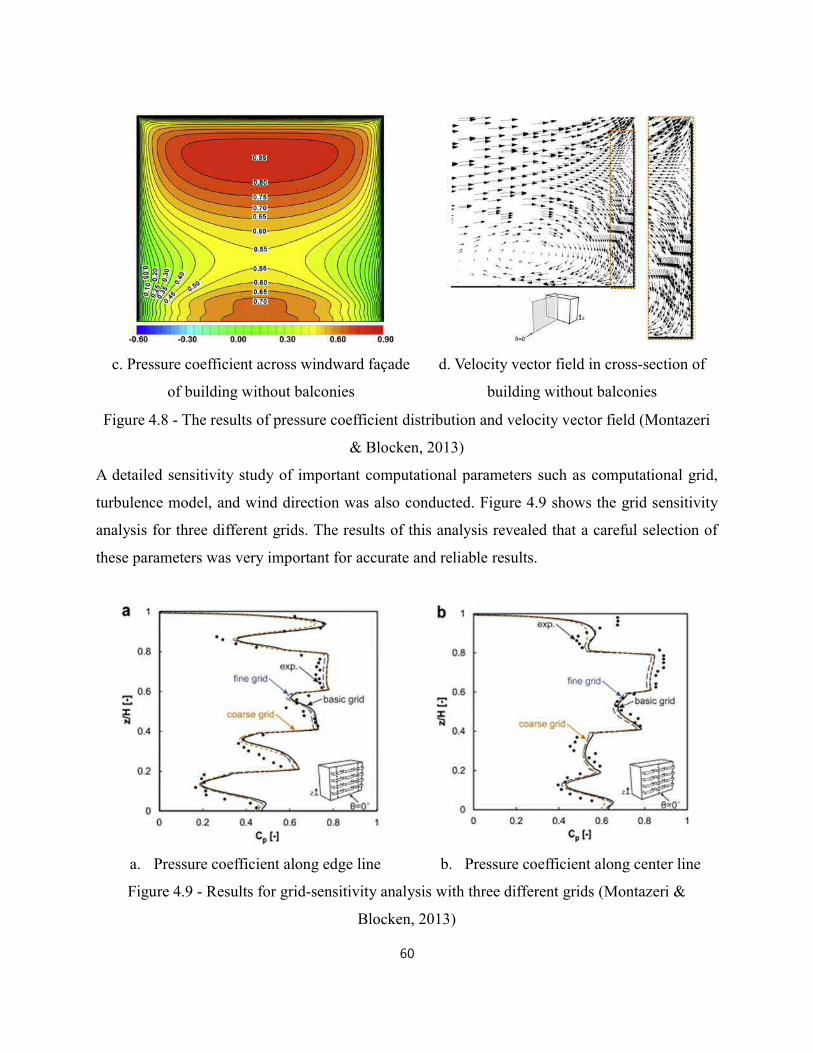
c. Pressure coefficient across windward façade

of building without balconies

d. Velocity vector field in cross-section of

building without balconies

Figure 4.8 - The results of pressure coefficient distribution and velocity vector field (Montazeri

& Blocken, 2013)

A detailed sensitivity study of important computational parameters such as computational grid,

turbulence model, and wind direction was also conducted. Figure 4.9 shows the grid sensitivity

analysis for three different grids. The results of this analysis revealed that a careful selection of

these parameters was very important for accurate and reliable results.

a. Pressure coefficient along edge line b. Pressure coefficient along center line

Figure 4.9 - Results for grid-sensitivity analysis with three different grids (Montazeri &

Blocken, 2013)

4.6. Lessons-learned from the journal article three: Effect of roof shape, wind direction,

building height and urban configuration on the energy yield and positioning of roof

mounted wind turbines (Abohela et al., 2013)


Roof mounted wind turbines have a high potential for integration within the built environment

but there is some uncertainty regarding their feasibility as a result of uninformed decisions about

positioning and locating the wind turbines. The factors that affect the installation of wind

turbines are wind directions, roof shapes, building heights and urban configurations.

This paper presented an investigation of air flow over a range of building roof shapes in order to

determine the most productive location in terms of power generated for a wind turbine using

CFD methods. The specific purpose of this study was to investigate the effect of different roof

shapes, wind direction, building height and urban configurations by examining the flow

characteristics in terms of wind flow patterns, turbulence intensities and streamwise velocities.



The study was intended to reproduce wind flow around buildings based on changes in several

parameters (roof shapes, wind directions, building heights and urban configurations). Thus, the

first resources were the modeled parameters. All roof shapes were designed to cover a building

with a square cross section of 6 m × 6 m and a height of 6 m. For the roof shape, the authors

(Abohela et al., 2013) used six different roof shapes: flat, domed, gabled, pyramidal, barrel

vaulted and wedged (Figure 4.10). For the wind directions, simulations were conducted with five

wind directions (0°, 45°, 90°, 135° and 180°). To understand the effect of building height on

wind flow above the building, three different heights were considered (6 m, 12 m, and 24 m).

Finally, two urban configurations were considered a street canyon and a staggered street.

The other resource was the commercial CFD software package and postprocessor Fluent 12.1.

This commercial code was applied over a wide range of options to examine the wind flow

around buildings. When the scaled residuals reached the range of 104 – 106, the simulations were

terminated.

Figure 4.10 - Roof shapes, from top left:

flat, domed, gabled, pyramidal, barrel vaulted and wedged (Abohela et al., 2013)


In the simulations the inlet boundary conditions were specified using a user defined function for

the log law ABL profile. For the ground surface, the standard wall functions for a rough wall

were used. The standard wall functions were also used for the surfaces of the building of interest.

Zero static pressure was applied at the outlet domain. Symmetry conditions, i.e. zero normal

velocity and zero normal gradients for all variables, were used at the top and lateral sides of the

domain. The realizable k- ɛ turbulence model was employed for the closure of the transport

equations and the SIMPLE algorithm scheme was used for the pressure-velocity coupling.

Pressure interpolation was second order and second-order discretization schemes were employed

for both the convection and the viscous terms of the governing equations.

The required outputs of the model were the values of the reattachment length on top of the roof

through variables such as roof shape, building height, wind direction and urban configuration. In

this paper, all flow features around a roof mounted cube in a turbulent channel flow were

captured including streamwise velocity pathlines and the pressure distribution passing through

the vertical central plane was as shown in Figure 4.11.

a. Stremwise velocity pathlines through the

vertical central plan

b. Streamwise velocity pathlines at ground

level

Figure 4.11 - The results of straemwise velocity pathlines and the pressure distribution

(Abohela et al., 2013)


For the computational domain, 2H + building width was utilized for the lateral dimension, 20H +

building dimension for the flow direction, and 6H for the vertical direction, where H is the height

of the building. Thus, a 126 m × 36 m × 36 m structured mesh was constructed, giving 1,306,368

hexahedral cells and maintaining a blockage ratio below 3%. Three mesh sizes were compared in

order to determine the dependence of the flow field on the refinement of the mesh. As a result, a

resolution of 0.3 m around the cube and 0.8 m throughout the rest of the computational domain

was established (Figure 4.12)

Figure 4.12 - Mesh refinement areas around the cube (Abohela et al., 2013)


This study investigated the effects of a large number of input parameters and conducted

sensitivity tests for the model results in order to help users make appropriate choices using the

commercial CFD code Fluent 12.1. However, the model in this study should still be applied by

CFD experts. Although there are CFD best practice guidelines that can assist non-CFD experts, a

knowledge of the physical models, potential computational errors or uncertainties should be

determined by CFD experts to ensure the correct application of the CFD model.

Generally, the process of generating additional meshes for mesh sensitivity analyses, the

representation of various models or additional geometries is very time consuming. For this study,

model flexibility was very important. The authors selected simple geometries that could easily be

made with structured mesh and once the proper mesh size was identified through a mesh

independence study, this was then applied to generate the meshes for all the parameters in this

study.


Conceptualization of the system refers to the processes that plot streamwise velocity pathlines

along the central plane on the roofs parallel to the wind direction for the most productive location

for a micro turbine. In the case of a building-integrated micro wind turbine and its location, it is

important when designing this structure to consider fully all aspects related to safety, structural

building integrity and turbine performance in order to achieve the maximum wind speed within

the built environment. Both the wind flow and turbulence intensity depend strongly on the roof

shape. Employing a CFD approach enables the air flow to be represented over a range of

common building roof shapes to achieve the most efficient location in terms of power production.

Prior knowledge for the system in this study includes the basic principles of physics in CFD such

as the conservation of mass, Newton’s second law and the conservation of energy and a

familiarity with the CFD best practice guidelines.


4.6.4.1. Modeling approach

The CFD approach adopted for this study was the best choice. The main reason is that four

factors affecting the location of the roof mounted wind turbines (six roof shapes, five different

wind directions, three building heights, and urban configuration) were modeled and flow patterns

visualized along the vertical streamwise central plane. Although this type of investigation has

generally been performed in a wind tunnel, the CFD approach is cost- effective and produces

more information than wind tunnel testing.

4.6.4.2. Conceptual model

As mentioned in Blocken and Gualtieri (2012), it is not efficient to attempt to include all the

physical processes involved and to encompass all possible combinations of meteorological

conditions. The model in this study therefore surveyed the scientific literature to identify

substantial simplifications. For the set of parameters to represent wind flows around buildings,

CFD best practice guidelines were adopted to achieve consistent results. Regarding the physical

processes and boundary conditions, the equilibrium ABL profile was modeled for the wind flow.


The variables of interest in this study are the streamwise velocity and the turbulence intensity.

From the streamwise velocity along the vertical central plane on the roof, the maximum

acceleration location can be determined. The relations between parameters can be expressed in

the form of partial differential equations. Generally, these equations can be solved using different

approaches (Blocken & Gualtieri, 2012); here, these equations were solved using the RANS

approach. The realizable k-ɛ turbulence model was used for the turbulence closure.


The purpose of this case study was to analyze wind flow over a range of common building roof

shapes to identify the most power productive location for building-integrated micro-wind

turbines. The authors addressed four main factors, namely roof shape, wind direction, building

height and urban configuration, that affect the installation of roof mounted wind turbines. The

model would be deemed successful if it was found to be capable of plotting the streamwise

velocity and the turbulence intensity along the central plane of the roof. Thus, the performance

criteria were the streamwise velocity and the turbulence intensity.


The knowledge gained from the literature and the CFD best practice guidelines was employed to

identify models and parameters. The authors selected the 3D RANS approach with the realizable

k-ɛ turbulence model for the closure of the transport equations due to its good performance for

the resolution of wind flows around buildings. The SIMPLE algorithm scheme was employed for

the pressure-velocity coupling. The pressure interpolation was second order and second-order

discretization schemes were used for both the convection and the viscous terms of the governing

equations (Blocken et al., 2010; Franke et al., 2007; Zhai & Chen, 2004).


For quantitative verification, comparisons of the pressure coefficient distribution along the

centerline of the windward, leeward façade and roof were conducted for data gathered from 15

wind tunnel tests, full-scale measurements and the CFD results. In this study, no qualitative

verification was conducted but its results could be presented to roof designers or scientists who

study renewable energy.


In order to reduce computational errors or uncertainties from model geometry, the mesh

generation, the choice of turbulence models, boundary conditions, and other factors, this case

study employed the CFD best practice guidelines. Hence, a range of 10-4 – 10-6 was applied for

the scaled residuals, and the choice of 3D RANS approach and the realizable k-ɛ turbulence

model, the computational domain size, the choice of the boundary conditions, the horizontal

homogeneity of the ABL profile, and so on were all based on the guideline recommendations.

Mesh independence analysis was conducted based on three different mesh sizes.


alternatives)

The purpose of this study was to investigate the effect of the roof shape, wind direction, building

height and surrounding urban configurations on the wind flow above the roof to identify the

optimum location where the accelerating effect occurs on top of the roof to maximize the energy

generation performance of a wind turbine. For the evaluation of the model, a qualitative analysis

of the streamwise velocities for the effects of different roof shapes was investigated (Figure 4.13).

In addition, comparisons of the turbulence intensities and velocities were carried out

quantitatively and quantitatively for the effects of building height and urban configuration

(Figure 4.14).

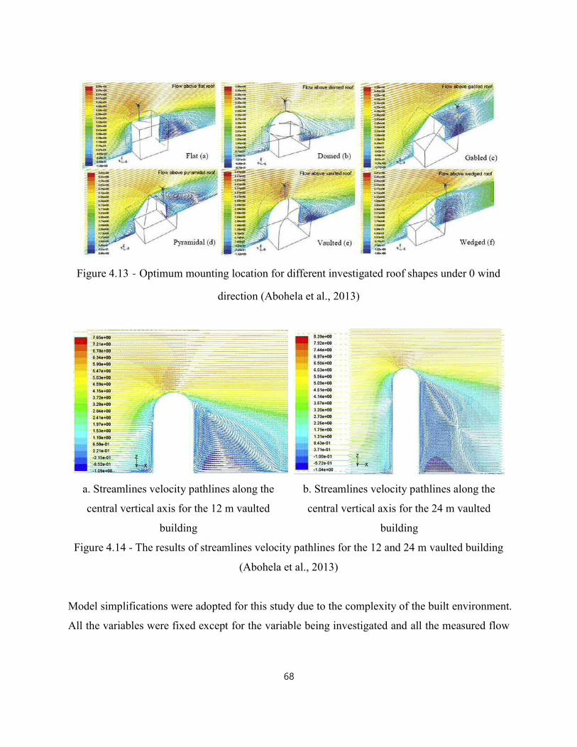
Figure 4.13Optimum mounting location for different investigated roof shapes under 0 wind

direction (Abohela et al., 2013)

a. Streamlines velocity pathlines along the

central vertical axis for the 12 m vaulted

building

b. Streamlines velocity pathlines along the

central vertical axis for the 24 m vaulted

building

Figure 4.14 - The results of streamlines velocity pathlines for the 12 and 24 m vaulted building

(Abohela et al., 2013)

Model simplifications were adopted for this study due to the complexity of the built environment.

All the variables were fixed except for the variable being investigated and all the measured flow

variables were normalized against the values of the flow variables at the same locations under

the same flow conditions in an empty domain to identify the accelerating effect of the roof shape.

In sum, this study concluded that the positioning of a roof mounted wind turbine requires careful

assessment of wind flow in order to maximize the energy extracted. The analyses carried out for

the study also increased our understanding of the accelerating effects of different variables on

wind flow across a roof.

4.7. Lessons-learned from the journal article four: Near-field pollutant dispersion in the

built environment by CFD and wind tunnel simulations (Chavez et al., 2011)


It is important to be able to assess pollutant concentrations in the built environment due to the

complexity of airflows around a multiple building configuration. When pollutants from roof

stacks become trapped in recirculation zones, this polluted air may re-enter the source building

as well as affecting adjacent buildings located downwind or upwind of the emitting building.

Although this re-entering polluted air is recognized to constitute a risk to human health, previous

studies have not provided appropriate design criteria to avoid this problem occurring in new or

existing buildings.

In this study, numerical simulations were conducted to reproduce pollutant dispersion within a

multiple building configuration. Specifically, this study investigated near field dispersion for

three different building configurations using CFD. The three different building configurations

were 1) a low-rise isolated building (emitting building); 2) a taller building placed upstream of

the emitting building; and 3) tall buildings placed upstream and downstream of the emitting

building. For the validation, the simulations results were compared with experimental results.

Another purpose of this study was to investigate the effect of different turbulence Schmidt

numbers on pollutant dispersion using CFD analysis.



For the investigations of pollutant dispersion, three resources were available for this study. The

first consisted of detailed building models for three different cases and the second was a set of

wind tunnel results (Stathopoulos et al., 2008) for comparison with the numerical results. The

other available resource was the commercial CFD code Fluent 6.1. For the building detail, three

cases were considered; the dimensions of the buildings are shown in Figure 4.15 and Table 4.3.

For all cases, it was assumed that the pollutant was released at the roof of B1.

Figure 4.15 - Three cases for CFD simulation (Chavez et al., 2011)

Table 4.3 - Building models for CFD and wind tunnel experiments (Chavez et al., 2011)

Building Height (m) Width (m) Length (m)

B1 0.075(15) 0.25(50) 0.25(50)

B2 0.15(30) 0.25(50) 0.15(30)

B3 0.27(54) 0.22(44) 0.075(15)

The wind tunnel experiments were conducted in the open circuit variable height boundary layer

wind tunnel of Concordia University by Stathopoulos et al. (2008). The dimensions of the wind

tunnel were 1.8 m × 1.8 m in section and 12.2 m in length and model buildings at a scale of

1:200 were used. A mixture of SF6 and nitrogen with a concentration of 10 ppm was released.

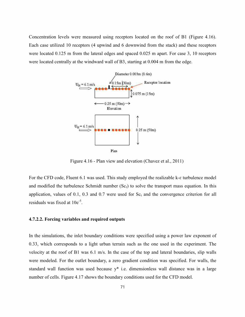
Concentration levels were measured using receptors located on the roof of B1 (Figure 4.16).

Each case utilized 10 receptors (4 upwind and 6 downwind from the stack) and these receptors

were located 0.125 m from the lateral edges and spaced 0.025 m apart. For case 3, 10 receptors

were located centrally at the windward wall of B3, starting at 0.004 m from the edge.

Figure 4.16 - Plan view and elevation (Chavez et al., 2011)

For the CFD code, Fluent 6.1 was used. This study employed the realizable k-ɛ turbulence model

and modified the turbulence Schmidt number (Sct) to solve the transport mass equation. In this

application, values of 0.1, 0.3 and 0.7 were used for Sct and the convergence criterion for all

residuals was fixed at 10e-5.


In the simulations, the inlet boundary conditions were specified using a power law exponent of

0.33, which corresponds to a light urban terrain such as the one used in the experiment. The

velocity at the roof of B1 was 6.1 m/s. In the case of the top and lateral boundaries, slip walls

were modeled. For the outlet boundary, a zero gradient condition was specified. For walls, the

standard wall function was used because y* i.e. dimensionless wall distance was in a large

number of cells. Figure 4.17 shows the boundary conditions used for the CFD model.

Figure 4.17 - Boundary conditions used for the CFD model (Chavez et al., 2011)

The required outputs for the model were the velocity and the dilution field. For the general view

of the results, the mean velocity magnitude of the vertical plane and the streamlines for the

middle vertical cross section and plane were presented to highlight differences in the velocity

field behavior. Contour lines for the dilution field were also presented to reveal the plume

behavior. Another required output was the normalized dilution for different values of Sct. The

authors expected to be able to predict pollutant dispersion based on the value of Sct for CFD

investigations.


The present study employed established CFD best practice guidelines for the computational

domain. For example, taking H as the building height of B1 (Case 1), the lateral and top

boundaries were 5 H away from building B1 and the outlet boundary was 20 H downwind. For

Cases 2 and 3, H was considered to be the building height of the tallest building. In order to

minimize the development of a streamwise gradient, a distance of 3 H away from the inlet to the

target building was employed. The dimension of this computational domain maintained the

blockage at 1.5 % in order to avoid any influence due to the lateral walls on the region of interest,

as recommended by the CFD best practice guidelines.

The computational model was constructed using a structured hexahedral mesh and the total

number of cells in the meshes ranged between 0.9 × 106 and 1.5 × 106 for Cases 1 to 3. The

expansion ratio between two consecutive cells was limited to 1.25. Figure 4.18 shows the mesh

for building B1.

Figure 4.18 - Perspective view of the mesh of isolated building case B1 (Chavez et al., 2011)


Although the commercial code, Fluent 6.1, provides a user-friendly interface for users, the

numerical model in this study needs to be handled carefully by the users. A knowledge of

aerodynamics, computational inputs for CFD analysis and the uncertainties of physical numerical

modeling, as well as an analysis of the grid sensitivity, were all required to obtain a correct

numerical modeling solution. Due to these requirements, this type of numerical study should be

carefully conducted by CFD experts.

The mesh sensitivity analysis examined three meshes: fine, medium and coarse. As the

comparison of normalized dilution in a specific point in the space showed very similar values for

the medium and fine meshes, the medium mesh was chosen by the authors. Regarding model

flexibility, this study only considered three different cases with up to three buildings. The stack

location was fixed on the roof of building B1 and the other buildings were just simple blocks.

Therefore, adding or removing meshes could be easily performed.


Conceptualization of the system in this study refers to the processes that affect pollutant

dispersion. In urban areas, effluents released from stacks located on the roof of a building can be

trapped in recirculation zones and may impact sensitive zones by re-entering the same building

or affecting an adjacent building. This can cause potentially serious health problems for the

occupants of the buildings.

Since previous studies showed that the turbulence Schmidt number (Sct) has a strong impact on

determining pollutant dispersion in the case of an isolated building. An assessment of the value

of Sct was therefore deemed important for the prediction of pollutant dispersion using CFD. Sct

is defined as the ratio of turbulent momentum diffusivity to mass diffusivity. Here, Sct values of

0.1, 0.3 and 0.7 were chosen based on the findings of previous studies (Blocken et al., 2008).

Prior knowledge for this system includes the fundamental physical principles of CFD such as the

conservation of mass, Newton’s second law and the conservation of energy.


4.7.4.1. Modeling approach

In order to assess pollutant concentration, a wide range of methods have been applied including

wind tunnel tests, field measurements, CFD and other semi-empirical models. However, most

available semi-empirical models are unable to solve near-field pollutant dispersion problems, and

wind tunnel and field measurements suffer from time and financial constraints. Thus, CFD

analysis was chosen in this case study. CFD has been widely used in studies of turbulent flow

and pollutant dispersion around buildings. It is expected to achieve whole flow data in order to

visualize flow and plume behaviors for qualitative analysis. Furthermore, it can easily provide

numerical data to permit the determination of Sct and hence analyze the effect of Sct on pollutant

dispersion.

4.7.4.2. Conceptual model

Based on a knowledge of the literature and considering wind tunnel measurements, substantial

simplifications were employed for this numerical study. For the model geometry, only three

simple block type buildings were considered and a single wind direction perpendicular to the

building was adopted. For the assessment of pollutant dispersion, ten receptors were placed

centrally along the windward wall of the rooftop.

4.7.4.3. Spatial and temporal scales

As mentioned earlier, this case study investigated pollutant dispersion in an urban area. For the

numerical model, structured hexahedral meshes were constructed except for the stack. Because

the stack had a circular cross-section, an unstructured wedge grid was used in this area. Within

the computational domain, a distinction can be made in spatial zones such as boundary

conditions.


The variables of interest in this study were the velocity and normalized dilution. The mean

velocity magnitude and streamlines for the three cases permit the flow behaviors to be visualized.

For normalized dilution, this can represent plume behavior such as that used for pollutant

modeling as well as comparing the effects of different values of Sct. The velocity can be

determined based on the physical laws of the conservation of mass, Newton’s second law and the

conservation of energy, all of which were established using partial differential equations. These

equations can be simplified using the RANS or LES approaches (Blocken & Gualtieri, 2012).

The value of Sct was based on previous studies (Blocken et al., 2008).


The main objective of this study was to reproduce the pollutant dispersion within a multiple

building configuration using a numerical approach such as CFD. Another objective was to assess

the effect of different values of Sct on pollutant dispersion. For the assessment of these

objectives, tracer concentrations from the CFD simulation results were used to obtain the

normalized dilution. This normalized dilution was also compared with wind tunnel results by the

authors and literature field results from Stathopoulos et al. (2008). It was also observed that

dilution was affected by the value of Sct, so the normalized dilution can be considered as a

performance criterion. Another criterion could be a qualitative comparison of the mean velocity

magnitude and the streamlines from the simulation results among the three cases.


According to Jakeman et al. (2006), this step is generally an iterative process of finding a

suitable model structure and parameter values. In this study, a 3D RANS approach was employed

rather than LES models. Although LES has been shown to provide a better agreement with

experimental results in pollutant dispersion, this requires computational resources about 100

times greater than those needed by steady RANS models. Among the RANS models, the

realizable k-ɛ turbulence model was selected because the value of Sct can be modified in this

model and it also exhibits much better agreement with experimental results than other steady

RANS turbulence models.


In this study, both qualitative and quantitative verifications were conducted. In the case of

qualitative verification, the mean velocity magnitude and contour lines of the dilution field for all

three cases were examined. For the quantitative verification, a comparison with measured data

was conducted in order to assess the effect of the value of Sct and the mesh sensitivity was also

analyzed.


Uncertainty in CFD modeling can arise from a very wide range of sources including the

simplification of model geometry, the mesh generation, the choice of turbulence models,

boundary conditions, and so on (Blocken & Guartieri, 2012). In order to reduce or avoid

uncertainties, this study employed the CFD best practice guidelines concerning the size of the

computational domain. The mesh sensitivity test was conducted based on three different meshes.


alternatives)

For the final step, the objectives of the model were evaluated. The main objective of this case

study was to reproduce near field pollutant dispersion for three different building configurations

using the CFD technique. For the model evaluation, a qualitative analysis was conducted. Among

the three cases, the mean velocity magnitude, the streamlines of the vertical cross-section and the

plan view, and the contours of normalized dilution were presented. For example, Figure 4.19

shows the concentration of the dilution for the three cases. This qualitative comparison shows

how the vortices interact with the surroundings and provide a better understanding of pollutant

dispersion within an urban area.

a. Case 1

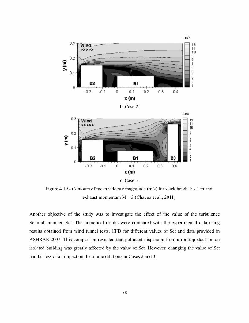
b. Case 2

c. Case 3

Figure 4.19 - Contours of mean velocity magnitude (m/s) for stack height h - 1 m and

exhaust momentum M – 3 (Chavez et al., 2011)

Another objective of the study was to investigate the effect of the value of the turbulence

Schmidt number, Sct. The numerical results were compared with the experimental data using

results obtained from wind tunnel tests, CFD for different values of Sct and data provided in

ASHRAE-2007. This comparison revealed that pollutant dispersion from a rooftop stack on an

isolated building was greatly affected by the value of Sct. However, changing the value of Sct

had far less of an impact on the plume dilutions in Cases 2 and 3.

4.8. Summary of lessons-learned from the journal analysis

Four journals were analyzed using the ten-iterative steps approach focusing on wind flow around

buildings in order to achieve the practical guidelines of CFD. Through the analysis, a rich

description of the CFD processes and lessons-learned were gathered:

Journal articles 1 and 4 used CFD to predict dispersion around an isolated building. While paper

1 was interested in comparing the RANS and LES models to obtain more credible results, paper

4 focused primarily on pollutant dispersion within multiple building configurations. In addition,

paper 2 investigated the pressure coefficients on buildings using CFD, while paper 3 conducted a

CFD analysis to understand the effect of various configurations in order to determine the

optimum position for roof mounted wind turbines.

Three of the papers (1, 2 and 4) reported conducting wind tunnel tests and using the data

collected to evaluate the CFD results. The specific size of the wind tunnel facility and the

velocity or pressure data measured in the wind tunnel, along with the boundary conditions, were

therefore available for the CFD simulations. In the case of paper 3, the specific conditions

utilized were those from earlier studies.

For the computational domain, all the studies created the domain recommended by the CFD best

practice guidelines (Franke et al., 2007; Tominaga et al., 2008). When H is the height of the

building of interest, the length of the upwind distance was 5H from the inlet domain and the

downwind length was 15H from the outlet boundary condition. For the vertical and lateral

dimensions, 6H was used for the height of the domain and 10H+w (where w is the building

width) was the lateral length. In the case of paper 4, distances of 3H for the upstream length and

20H for the downstream length were used.

All studies utilized structured hexahedral meshes except paper 2, which generated a hybrid mesh

composed of both hexahedral and prismatic cells. All four studies performed the grid sensitivity

analysis with three different grid densities in order to identify the proper mesh size. Three

meshes, namely fine, medium and coarse, were generated for each analysis.

For the boundary conditions, the commonly measured vertical wind profile from the experiments

was applied as the inlet boundary condition. In order to specify the velocity profile of the

atmospheric boundary layer at the inlet, two kinds of expression are used. One is a log-law and

another is a power law (Huang et al., 2007). Between these two expressions, the power-law

velocity profile has been generally used when the experimental data is not available (Ai & Mak,

2013). While papers 2 and 3 employed a log-law, paper 4 used a power-law for the inlet

condition, and paper 1, used both log-law and power-law for their RANS and LES approaches,

respectively. For the top and lateral boundary conditions, papers 2 and 3 used symmetry

conditions while paper 1 used no-slip conditions and paper 4 used slip wall conditions for the top

and lateral sides of the domain. In the case of the outlet boundary conditions, most of the studies

assumed a zero static pressure condition. For the ground surface, the standard wall functions as a

rough wall were applied by all the studies.

For all four sets of researchers, the velocity components were the common variable of interest.

This parameter can be expressed in the form of partial differential equations (see Chapter 2).

Generally, these equations can be solved using either the RANS or LES approaches. Papers 2, 3,

and 4 employed the RANS approach with the realizable k-ɛ turbulence model for the closure

while paper 1 employed both the RANS with the RNG k-ɛ turbulence model and LES

approaches in order to compare the accuracy of the results of these models.

In papers 2 and 3, the SIMPLE algorithm was employed for the pressure-velocity coupling, the

pressure interpolation was second order and second-order discretization schemes were employed

for both the convection terms and the viscous terms of the governing equations. In addition, most

of the studies assumed that convergence was obtained when all the scaled residuals leveled off

within the range of 104 – 106.

After convergence had been obtained, the outputs for all the articles consisted of all the

parameters of the average flow field around the building of interest. The velocity or pressure

field and other simulations results were generally represented through the research purpose. In

the case of paper 1, the wind velocity and instantaneous fluctuations of concentration at the

building surfaces were the criteria and these criteria were validated with wind tunnel data in

order to identify the preferred turbulence model between the RANS and LES methods. The

purpose of paper 2 was to predict the pressure distribution on a building with and without

balconies using a 3D RANS approach. Thus, the target criteria of this paper consisted of the

pressure distributions on the building surface, which were also validated with experimental data

and then used to investigate the impact of computational parameters. For paper 3, the streamwise

velocity and turbulence intensity were used to investigate various options for roof shape, wind

direction, building height and urban configuration in order to identify the most productive

location for power generation by building-integrated wind turbines. Finally, paper 4 conducted

CFD simulations to predict pollutant dispersion within buildings. The results of this study were

expressed in terms of the mean velocity magnitude and the streamlines.

The final step was to evaluate the objectives of each journal article. For paper 1, the main

objective was to investigate the accuracy of LES for the reproduction of dispersion around a

building. Through the various comparisons, LES showed better agreement with experimental

data and provided more important information than the RANS approach that was also tested.

However, this came at a cost; the computation time for LES was significantly longer than that of

the RNG k-ɛ model. The objective of paper 2 was to reproduce wind pressure distributions

across building facades with balconies. Here, only a steady RANS approach with the realizable

k-ɛ turbulence model was employed and the results compared with wind tunnel data. Good

agreement was obtained between CFD and wind tunnel tests and the sensitivities of

computational parameters such as grids, turbulence models and wind direction were analyzed.

The authors concluded that the careful selection of computational parameters was very important

to ensure the accuracy and reliability of the results. In the case of paper 3, the objective was to

investigate the effect of roof shape, wind direction, building height and surrounding urban

configurations on the wind flow above the roof. Employing the RANS approach with the

realizable k-ɛ turbulence model, the streamwise velocities for the effects of different roofs shapes

were analyzed qualitatively and comparisons of the turbulence intensities and velocities were

conducted quantitatively to examine the effects of different building heights and urban

configurations. Finally, the objective of paper 4 was to reproduce near field pollutant dispersion

within three different building configurations using the RANS approach with the realizable k-ɛ

turbulence model. The mean velocity magnitude and the streamlines were presented for

qualitative analysis and the numerical results of the concentration were compared with wind

tunnel data.

As described above, the description of the CFD process and lessons-learned were obtained

through the journal analysis. These findings can be helpful to assist designers and architects to

utilize CFD in the architectural design process. By considering these findings, the practical

computational parameters for wind flow around buildings were achieved and summarized in

table 4.4.

Table 4.4 - A summary of lessons-learned: the computational parameters for wind flow around

buildings

The computational

domain size

- 5H and 15H for the length of upwind and downwind length respectively (when H is the height of the building of interest)

- 6H for the vertical extension -10H+W (where, w is the building width) is for the lateral length

Grid type

and resolutions - Hexahedral meshes were used. - Three different grids were constructed.

Boundary conditions - The experimental data were specified at the inlet using power law and logarithmic law.

- A zero static pressure condition was imposed at the outlet - For the sides and tops, symmetry conditions were used. - The standard wall functions were used for wall boundaries.

Turbulence models - Two RANS approaches (the Realizable k-ɛ and the RNG k-ɛ). - LES model was also considered for the accuracy.

Algorithm and scheme - The SIMPLE algorithm and second-order discretization schemes

Convergence criteria - All the scaled residuals leveled off within the range of 104 – 106.

5. WIND TUNNEL TESTING

In general, wind tunnels have been used to study the flow of air over objects of interest, the

forces acting on them and their interaction with the flow. Nowadays, wind tunnels are employed

to verify aerodynamic studies in a wide range of applications, including in the automotive

industry, architecture, environment, and education. While the use of numerical approaches such

as CFD has increased, wind tunnel tests are still important for developing new aircraft, wind

turbines or other designs that involve complex interactions with the flow (Hernández et al., 2013).

In the case of architecture, the effects of aerodynamic forces on buildings and structures must

also be considered for structural stability (English, 2007).

5.1. Architectural applications of wind tunnel testing

Wind tunnels have been used to determine the aerodynamic characteristics of buildings for a

number of years (Zhang & Gu, 2008). In recent examples, Yasui et al. (2002) performed wind

tunnel tests, full-scale observation and CFD to investigate wind pressures on tower-like

structures, while Lo et al. (2013) conducted a combined approach with CFD and wind tunnel

testing for indoor airflow prediction of wind-driven cross ventilation. To predict dispersion in a

street canyon with tree planting, Gromke et al. (2008) conducted both wind tunnel tests and

numerical investigations and Wong and Heryanto (2004) investigated an active stack effect for

improving natural ventilation by means of wind tunnel and CFD simulations. Recently, the use of

wind tunnel studies has been increasingly applied for building applications (Cochran &

Derickson, 2011).

5.2. Overview of wind tunnel testing at IBHS

Wind tunnel tests were performed to characterize the innovative vent system developed by

Virginia Tech and Acrylife Inc. at the wind facility belonging to the Institute for Business and

Home Safety (IBHS) in Richburg, SC. This wind tunnel testing was assisted by Acrylife and

Radco Construction. Pressures were measured under the roof membrane and initial tests without

the membrane were conducted to gather baseline data on pressure magnitudes and distributions

on the roof surface. After the initial measurements, tests were performed with up to two roof

vents, a parapet vent system, and parapet walls. Wind speed data from a reference anemometer at

an elevation of 13 ft and pressure readings recorded at each of the roof pressure taps were stored

at the IBHS (Morrison et al., 2012b).

5.2.1. The IBHS wind facility

The Insurance Center for Building Safety Research (ICBSR) was created by the Institute for

Business & Home Safety (IBHS) to provide a unique research center that can test low-rise

buildings subjected to a variety of natural hazards as well as other types of losses. The main

facility is a large open-jet wind tunnel that can subject full-scale one or two-story buildings to

high winds accompanied by wind-driven rain, hail and even fire. Testing in the facility includes

the ability to rotate building orientation relative to the wind direction, change vanes to generate

lateral turbulence, introduce rain drops with prescribed distributions of droplet sizes and rainfall

rates, inject burning embers of various sizes, and simulate hailstones. The research conducted at

the IBHS improves our understanding of the interaction between extreme winds and buildings.

Moreover, it provides information on the weaknesses of residential buildings and building

systems subjected to natural storms as well as offering opportunities to improve construction

techniques and building component design and manufacturing. It also influences public policy

such as building code development (Liu et al., 2009).

a. Aerial photograph of the IBHS Research

Center b. 105 fans of the Inlet

Figure 5.1 - IBHS Research Center in Richburg, SC (Morrison et al., 2012a)

Figure 5.2 - Plan view and elevation views of the IBHS facility (Liu et al., 2009).

5.2.2. Facility details of the IBHS

The test chamber in the wind tunnel is 145’ (44.2 m) wide × 145’ (44.2 m) long, with a clear

interior height of 60’ (18.3 m). Since the length is relatively short, this facility cannot reproduce

the mean and turbulence characteristics of the atmospheric boundary layer. Due to this limitation,

this facility uses both active and passive control elements. One hundred and five 5.5’ (1.68 m)

diameter vane-axial fans with 350 horse power medium voltage electric motors are used to

produce the wind flow. The array for these fans is divided into 15 cells placed in a grid 5 cells

across and 3 cells high. As shown in Figures 5.3 and 5.4, the contraction from the fans to the

inlet is approximately 2:1 and the size of the inlet has dimensions of 65’ (19.8 m) × 30’ (9.1 m).

The speed of each fan cell is independently operated by a programmable logic controller (PLC)

capable of updating the running speed of the fans at a maximum frequency of 4 Hz. The

directional wind vanes and spires can also be used to control the fan speed to develop appropriate

flow characteristics to reproduce the ABL. There are 16 wind vanes extending the entire height

of the inlet. These vanes are divided into five groups capable of rotating independently of each

other at angles of between -15° to +15°, with 0° representing the streamwise direction. The

movement of the wind vanes produces large-scale flow fluctuations in the lateral direction. In

order to produce turbulence at higher frequencies than are possible by modulation the fan speeds

alone, spires are used to alter the mean flow profile within the lower and middle cells. A 55ft

diameter turntable within the test chamber can be used to rotate the structural test specimens

remotely (Morrison et al., 2012a).

Figure 5.3 - Wind vanes at the inlet of the IBHS wind facility

Figure 5.4 - Layout of the IBHS Research Center test chamber and inlet from the fans

(Morrison et al., 2012a)

5.3. Experimental configuration

The data used in the current study were acquired during experiments performed at the IBHS

wind tunnel facility. The overall view of the test building is shown in Figure 5.5. The test

building was 30ft × 40ft in size, with a height of 13ft, and located 26ft downstream from the inlet.

The test building was furnished with 158 pressure taps. The pressure scanning system used in the

experiment measured all the pressures almost instantaneously. The pressure taps were located on

the left windward quadrant of the roof, as shown on the plan view of the instrumented module

sketched in Figure 5.6. These tap locations were developed as part of IBHS testing of root top

equipment (Morrison et al., 2012b). The density of pressure taps was higher close to the

windward sides of the roof, where larger pressure variations were expected and the tap line

closest to the roof edge was at y/H = 0.038. In the tests, a 900 s sample with 100 Hz sampling

rate was recorded as a time series for every tap at 6 approaching wind angles: 0°, 15°, 30°, 45°,

60° and 90°.

a. Test building

b. Layout of the test building and the chamber

Figure 5.5 - The overall view of the wind tunnel facility

The reference velocity was monitored using a RM Young anemometer at roof height. The

obtained surface pressure data were converted to the non-dimensional pressure coefficient Cp

using:

Pressure coefficient (Cp) is defined as the non-dimensional ratio which describes the relative pressures throughout a flow field.

Cp � � � ��0.5�� Equation 5.1 – Calculation of the pressure coefficient

where P is the average pressure measured on each tap on the surface, P∞ is the static pressure

within the test chamber and V is the 15 minute mean velocity at roof height (Morrison et al.,

2012a).

1.5 1.25 2

0

2.5

5

7.5

10

12.5

15

17.5

20

22.5

2.5 5 7.5 10 12.5 15 17.5 20 22.5

30

4022.5

17.5

22.5 7.5

11

2 21.251 1 1.25 1.25 1.25

1.51.5

1.5

2.51.75

1.51.5

2

2.52.5

2.25

2 2 2 2 2 2 2 2 2

Figure 5.6 - The location of the pressure taps on the roof of the test building

In addition, the mean wind velocity profile and the longitudinal intensity profiles (Iu) were

provided for this study. These measurements were previously conducted in order to provide

realistic predictions of the performance of full-scale structures at the IBHS facility. The data

obtained were compared with field data provided by Texas Tech University. According to the

report by Morrison et al. (2012a), the mean velocity profile and the longitudinal and lateral

turbulence intensity profiles showed good agreement with both field measurements and

theoretical profiles. Among the data obtained, the mean velocity and longitudinal turbulence

intensity profiles were used to determine the turbulent kinetic energy and turbulent dissipation

rate for the CFD modeling (Figure 5.7).

Figure 5.7 - Mean velocity (left) and longitudinal turbulence intensity (Iu) (right) profiles

(Morrison et al., 2012a)

For the evaluation of roof vent performance, pressures on the roof surface were measured. First,

tests were conducted with no membrane on the roof surface at various wind angles. Second,

measurements were performed with the membrane in place. After investigating the pressures

with and without the membrane, two roof vent systems were installed at two locations and the

effect of a parapet vent system was also investigated.

5.4. Results

A number of different experimental configurations were investigated at the IBHS wind facility.

All pressure data were acquired and analyzed by IBHS staff (Morrison et al., 2012b), who

provided the results as contour plots of non-dimensional pressure coefficients. While

experiments with various configurations were conducted, pressure data measured on the roof

surface without the membrane were selected for this study. Since one of the purposes of this

study was to gather a rich description of the CFD process that can be achieved by validation with

experimental data, a simple geometry was used when performing CFD simulation in an attempt

to avoid numerical errors or uncertainties. Thus, the mean surface pressures on the roof deck

without the membrane at a wind angle of 0 degrees were chosen for the validation with CFD.

Figure 5.8 - Pressure coefficient distribution on the roof surface (Morrison et al., 2012b)

Figure 5.8 shows the distribution of the non-dimensional pressure coefficients on the roof surface

without a membrane. The reference wind speed at the building height was 46.2 mph (20.69 m/s).

According to Figure 5.9, the mean pressure coefficients near the edge of the roof were relatively

lower and the pressure coefficients generally increased along the centerline of the roof surface.

This indicates that the highest suction occurred near the edge, decreasing as it progressed along

the centerline.

Figure 5.9 - Pressure coefficient distribution along the centerline on the roof surface

For the CFD analysis, the geometry of the building of interest was employed to create a

computational domain. The wind tunnel data for the rooftop sensors was used for grid sensitivity

tests and the validation. The detailed comparison with the CFD results will be presented in

Chapter 7.

Pres

sure

Coe

ffici

ent

Distance along centerline on the roof of the test building (ft)

6. THE SENSITIVITY ANALYSIS

6.1. Introduction

Based on the document analysis described in Chapter 3 and 4, several computational parameters

were chosen. The selected computational parameters and their influence on CFD analysis are

described in this chapter through the sensitivity analysis. The sensitivity of three computational

parameters including the computational domain size, the grid size and turbulence model was

tested and all the sensitivity analyses employ the same geometry as the wind tunnel testing at the

IBHS.

6.2. Context of the wind tunnel tests at the IBHS

For the sensitivity analysis, the wind tunnel tests with a full-scale building at the IBHS wind

facility were reproduced using the CFD simulation. The purpose of the wind tunnel tests and the

details of the wind facility and the experimental configurations were described in Chapter 5.

The dimensions of the wind tunnel facility are 145 ft long by 145 ft wide, with a height of 60ft.

Although this facility cannot reproduce the mean and turbulent characteristics of the atmospheric

boundary layer due to its short length, the speed of each of its 105 350 horse power fans can be

adjusted by a programmable logic controller to reproduce the conditions typically experienced in

the atmospheric boundary layer.

Inside the chamber, a 30 ft by 40 ft, 13 ft tall, test building was placed 26 ft downstream from the

inlet. The test building was furnished with 163 pressure taps on the left windward quadrant of the

roof. Various experimental configurations were investigated and pressure data obtained using the

pressure taps. During these tests, a 15-min mean speed of the order of 40 - 45 mph was achieved.

In addition, the mean velocity and longitudinal turbulence intensity profiles measured for the

previous experiments were employed to obtain the turbulent kinetic energy and turbulent

dissipation rate for the inlet boundary condition.

Among the various configurations tested in the original wind tunnel experiments, wind flow on

the roof surface without a membrane was selected for the CFD modeling. Since this test had the

simplest geometry, with no extraneous features such as parapet walls, membranes, or vents, this

configuration was selected in order to facilitate the CFD simulation. The obtained pressure data

were used to investigate the impact of computational parameters.

6.3. Other computational parameters

Although the sensitivity analysis investigates the impact of the computational domain size, the

grid density and the selection of turbulence model, respectively, it is necessary to clarify a

number of other computational parameters including initial conditions, discretization methods,

boundary conditions, solution algorithms, and convergence criteria in order to perform the CFD

analysis. According to the guidelines laid out by Casey & Wintergerste (2000), the parameters

for the control of convergence of the solution algorithm, including the relaxation factor, damping

factors or time steps as recommended by the commercial CFD code, can be used. In addition, the

commercial code provides useful parameters or conditions for non-experts to help them conduct

a successful CFD analysis, the default settings of the commercial code were employed for this

study (Bakker et al., 2001). Other computational parameters of best practice guidelines and the

analysis of journal articles (Chapter 3 & 4) were used.

6.4. Investigations of wind flow on a roof with three different computational domain sizes

6.4.1. Problem statement

To maximize the accuracy of the CFD simulation, it is important to determine the size of the

entire computational domain in the vertical, lateral and in/out flow directions. In general, the

recommendations of the best practice guidelines by Franke et al. (2007) and Tominaga et al.

(2008) were employed to create the computational domain. However, the upstream length of the

wind tunnel was only 2H, which was smaller than the recommendations of the best practice

guidelines, where H is the height of the building of interest. In addition, Ramponi and Blocken

(2012) observed that the blockage ratio also influences the results of CFD.

For this study, the sensitivity of three different computational domain sizes was investigated. For

the reference model, 5H for the upstream length and 15H for the downstream length were

employed. For the lateral and vertical domain lengths, the height and width of the wind tunnel

were used. As mentioned previously, 2H was the upstream length for the first test model. Other

conditions were the same as the reference model. For the second test model, an increased

blockage ratio was employed to compare the effect of the blockage ratio.

6.4.2. Computational domain

As described above, a full-scale building in a wind tunnel was modeled explicitly, satisfying the

best CFD practice guidelines requirements for upstream and downstream length as a reference

model. In addition, two other computational domain sizes were also constructed. For all

computational domains, the upstream length was kept as short and the length of downstream was

set long enough to allow the development of the wake region behind the building and thus

support the convergence of the simulations (Blocken et al., 2012). For the reference model, the

domain dimensions were L × W × H – 307 ft × 145 ft × 60 ft (93.7 m × 44.2 m × 18.3 m). In the

wind tunnel tests at the IBHS, the upstream length from the inlet boundary to the test building

was 2H (26 ft) and the blockage ratio was 4.5 %. In order to investigate the impact of upstream

length on the results of CFD, an upstream length of 2H was also applied for the first model; the

dimensions L × W × H – 268 ft × 145 ft × 60 ft (81.7 m × 44.2 m × 18.3 m) were applied. Franke

et al. (2007) recommended a maximum blockage of 3% but used the same cross-section of the

wind tunnel for the computational domain. Thus, the blockage ratio of the reference model was

4.5%. In order to compare the effect of the blockage ratio, a blockage of 6.8 % was applied to the

second model. When the height of the building is H, Hd is the height of the computational

domain and this can be expressed as Hd – H + d. For the lateral extension, W is the test building’s

width and Wd is the width of the computational domain. Wd can be expressed as Wd – W + 2d.

While 5H was used for the vertical and lateral extension in order to avoid any interference of the

domain size on the numerical results (Ramponi & Blocken, 2012), 3H was employed with a

blockage ratio of 6.8% in order to investigate the impact of the blockage ratio, thus reducing the

computational domain size. The dimensions of the second model were L × W × H – 307 ft × 109

ft × 52 ft (93.7 m × 33.2 m × 15.8 m). The three domains are presented in Figure 6.1.


The grid was constructed based on the recommendations made by Franke et al. (2007) and

Tominaga et al. (2008). The grid for the three cases consisted solely of hexahedral cells. While a

considerable effort was required to generate a hexahedral mesh, this type of grid avoids the well-

known convergence problems associated with hybrid grids that include tetrahedral cells (Blocken

et al., 2012). For this grid, a second-order discretization scheme was used, as recommended by

Franke et al. (2007). This option is set as the default in the commercial code STAR-CCM+8.04

and this scheme is considered the most accurate for steady-state calculations (STAR-CCM+

UserGuide 8.04).

For the reference model, 682,380 cells were created using the generating mesh tool in STAR-

CCM+ 8.04. For the first model for the evaluation of effect of the upwind length, 606,008 cells

were constructed. The final model for the investigation of the effect of the blockage ratio

consisted of 393,456 cells.

a. Computational domains for the reference model

b. Computational domains for the model with 2H of the upstream length

c. Computational domains for the increased blockage ratio model

Figure 6.1 - Three different computational domains


In order to obtain a better agreement between the experimental and numerical results, the

boundary conditions adopted in the CFD simulation should be the same as those measurements,

especially for inflow boundary conditions (Huang et al., 2007). For this study, the atmospheric

boundary layer inflow was created at the inlet. The inlet boundary conditions, including the mean

velocity, turbulent kinetic energy and turbulence dissipation rate, were based on the measured

incident vertical profiles of mean wind speed and longitudinal turbulence intensity. The mean

wind speed profile was prescribed by the power law with an exponent of 0.143, which

corresponds to an open land surface. The velocity at the test building height was 20.69 m/s (46.3

mph). The estimated turbulence intensity, the inlet value of turbulence kinetic energy, k, and the

turbulence dissipation rate, ɛ are given by Equations. 6.1 and 6.2:

k � �� Equation 6.1 – Calculation of the turbulence kinetic energy

ɛ � � �/� ��/�

� Equation 6.2 – Calculation of the turbulence dissipation rate

where Uavg is the mean velocity at the inlet, I is the turbulence intensity, Cμ is an empirical

constant specified in the turbulence model (~ 0.09), and l is the turbulence integral length scale.

These values are presented in Figure 6.2. These values can be specified at the inlet in order to

obtain a better agreement between experiments and CFD.

Based on reports in the literature (Blocken et al., 2012), symmetry boundary conditions were

applied for the sides and the top of the computational domain that assumed zero normal velocity

and gradients. For the outlet condition, a static pressure of zero was defined. Within the

computational domain, no-slip wall boundary conditions were applied for the surfaces of the test

building.

U/U10

Z(m

)

Z(m

)

K (m2/s2)

a. The mean wind speed profile by power law b. Turbulence kinetic energy k

Figure 6.2 - The inlet boundary conditions

6.4.5. Other computational conditions

The commercial code STAR-CCM+ 8.04 was employed for this CFD simulation with the 3D

RANS equations. The realizable k-ɛ turbulence model was used for the analysis of wind flow

around a building and the choice for this turbulence model was based on earlier successful

validation studies for wind around a building (Blocken et al., 2012; Montazeri et al., 2013;

Janssen et al., 2013). Steady state calculations were performed using the SIMPLE algorithm with

a second-order discretization scheme for convection terms and viscous terms of the governing

equations. When the residuals reached 105 for the velocities of x, y, and z, 105 for k and ɛ, and

105 for continuity, the iteration process ended.

6.4.6. CFD simulation results

6.4.6.1 Qualitative comparisons

First, the results of the computations in terms of velocity were analyzed for all three models.

Figure 6.3 shows a comparison of the predicted mean velocity magnitude for the middle vertical

plane. According to this comparative view of the results, the wind flow patterns in three cases are

similar. Although the upwind flow of the second case is stronger than that in two other cases, a

large difference among three cases is not observed.

As shown in Figure 6.4 and Figure 6.5, contours of mean velocity magnitudes and pressure

coefficients distribution on the roof surface of each case are presented. Similar to the

comparisons in Fig 7.3, the result of the reference model shows the similar patterns with the two

other cases. Overall, the effect of the shorter upstream length and the increased blockage ratio on

both the velocity and pressure field is small.

a. The reference model

b. 2H of upstream length

c. The increased blockage ratio

Figure 6.3 - Contours and vectors of mean velocity magnitude for the middle vertical plan




Figure 6.4 - Contours of mean velocity magnitude on the roof surface




Figure 6.5 - Contours of pressure coefficients distribution on the roof surface

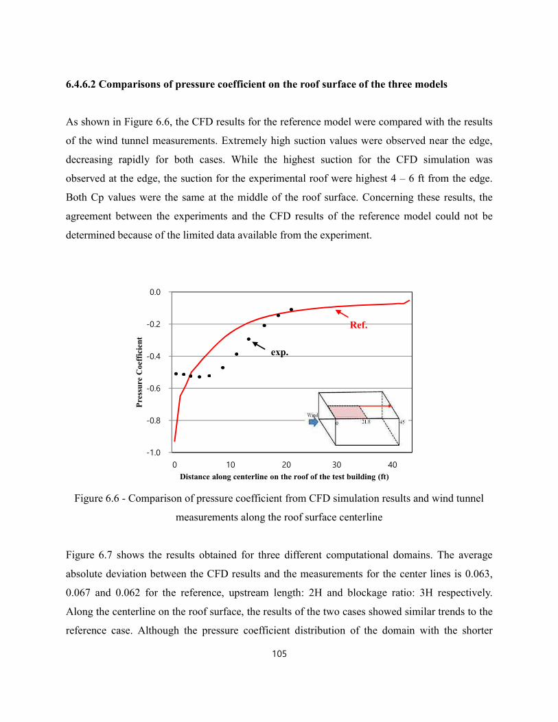
6.4.6.2 Comparisons of pressure coefficient on the roof surface of the three models

As shown in Figure 6.6, the CFD results for the reference model were compared with the results

of the wind tunnel measurements. Extremely high suction values were observed near the edge,

decreasing rapidly for both cases. While the highest suction for the CFD simulation was

observed at the edge, the suction for the experimental roof were highest 4 – 6 ft from the edge.

Both Cp values were the same at the middle of the roof surface. Concerning these results, the

agreement between the experiments and the CFD results of the reference model could not be

determined because of the limited data available from the experiment.

Figure 6.6 - Comparison of pressure coefficient from CFD simulation results and wind tunnel

measurements along the roof surface centerline

Figure 6.7 shows the results obtained for three different computational domains. The average

absolute deviation between the CFD results and the measurements for the center lines is 0.063,

0.067 and 0.062 for the reference, upstream length: 2H and blockage ratio: 3H respectively.

Along the centerline on the roof surface, the results of the two cases showed similar trends to the

reference case. Although the pressure coefficient distribution of the domain with the shorter

Pres

sure

Coe

ffici

ent


exp.

Ref.

upstream length was lower than the other cases, the results of all three cases showed a small

change in pressure distribution.

Figure 6.7 - Impact of the computational domain size on CFD simulation results for the

pressure coefficient along the roof surface centerline

6.4.7. Discussion

This study focused on the validation of the results between CFD and wind tunnel tests,

specifically investigations of CFD simulations of wind flow on the roof surface and the impact of

three different computational domain sizes. The main conclusions can be summarized as follows.

First, the results of the CFD simulation were compared with the wind tunnel tests. Both cases

showed that high suction occurred near the edge. However there was a discrepancy in the Cp

values of both cases near the edge, probably because of the characteristics of the RANS

turbulence model. For this study, the realizable k-ɛ turbulence model was employed, based on

reports in the literature. According to the study by Abohela et al. (2013), a comparison of

exp.

upstream:2H

BR:3HRef.

pressure coefficients of published in-situ measurements, wind tunnel tests and validated CFD

simulations (Figure 6.8) revealed similar patterns for both CFD and wind tunnel tests. Thus, the

discrepancy in the results of the current study was likely caused by the RANS turbulence model

and it is thus necessary to examine the impact of different turbulence models.

Figure 6.8 - Comparison of pressure coefficients along the centerline of the windward façade,

roof and leeward façade with the average of the 15 wind tunnel tests, the Silsoe 6 m cube full

scale measurement and CFD simulation (Abohela et al., 2013)

The results of the examination of the impact of different computational domain sizes confirmed

that the wind flow behavior was indeed affected by the size of the computational domain.

Compared with the reference model, the impact of the shorter upstream length was more

significant than the increased blockage ratio. However, all three cases showed only a small

change in the Cp values. This seems to indicate that the different computational domains were

not highly sensitive to the results of CFD simulation.

6.5. The sensitivity analysis of the impact of the computational grid resolution


With regard to the generation of the computational grid, the discretization method must be

specified to ensure that the grid is created in such a manner that it does not cause errors that are

too large. This means that its resolution has to be fine enough to capture important physical

phenomena such as shear layers and vortices with sufficient resolution (Franke et al., 2007). As

mentioned earlier, as the number of cells increases, the accuracy of the simulation also increases

but at the cost of extremely high computer memory requirements. Therefore, it is important to

determine the optimum size of mesh. Casey & Wintergerste (2000) suggested the analysis of grid

sensitivity to ensure the suitability of the mesh in CFD simulations.

Three different discretization methods may be used: the Finite Volume, Finite Difference and

Finite Element methods. Among these, the Finite Volume method was selected for this study

because it has been widely used in commercial codes and micro-scale obstacle accommodating

meteorological models (Franke et al., 2007). With the Finite Volume method, three significantly

different grid resolutions were generated for the grid sensitivity analysis in an attempt to reduce

both discretization errors and computation time. For the reference model used in the first case

study, 682,380 cells were created for the reference model, along with a coarser grid and a finer

grid. The grid sensitivity analysis was performed in order to determine how grid density

influences the results of the CFD simulation and the impact on the accuracy of the CFD.


As in the first sensitivity test in Section 6.4, a full-scale building in the wind tunnel was modeled.

Satisfying the best CFD practice guidelines, the upstream length was 5H and the downstream

length was set as 15H, with H as the height of the test building. The vertical and lateral distance

from the test building were the same as the wind tunnel. Thus, the domain dimensions of the

reference model were L × W × H – 307 ft × 145 ft × 60 ft (93.7 m × 44.2 m × 18.3 m), with a

blockage ratio of 4.5%. In the computational domain, the building of interest was located 26 ft

from the inlet boundary.


The grid was created following the recommendations made by Franke et al. (2007) and

Tominaga et al. (2008). In addition, the second-order discretization scheme recommended by

Franke et al. (2007) was utilized. The grids for the reference, coarser and finer models were

constructed entirely of hexahedral cells. The three grids are illustrated in Figure 6.9. The three

grids were constructed by increasing the resolution by about a factor of 2 (Ramponi & Blocken,

2012). The grid for the reference model consisted of 682,380 cells, the coarse grid had 98,510

cells, and the fine grid had 1,590,548 cells.


The same boundary conditions as used in the first sensitivity test were also applied for the second.

At the inlet boundary condition, the measured vertical velocity profile was applied and the

turbulence kinetic energy k, and dissipation rate ɛ were specified. For the outlet boundary

conditions, zero static pressure was defined. Symmetry boundary conditions were applied for the

sides and the top of the computational domain, which again assumed zero normal velocity and

gradients. No-slip wall boundary conditions were applied for the surfaces of the test building in

the computational domain.

a. The reference model: 682,380 cells

b. The coarse grids: 98,510 cells

c. The fine grids: 1,590,548 cells

Figure 6.9 - Three different computational grids for grid-sensitivity analysis


The commercial code STAR-CCM+ 8.04 was employed for this CFD simulation, along with the

3D RANS equations. The realizable k-ɛ turbulence model was used for the analysis of wind flow

around the building. Steady state calculations were performed using the SIMPLE algorithm with

a second-order discretization scheme for convection terms and viscous terms of the governing

equations. Convergence was obtained when the scaled residuals reached a minimum of 105 for

the velocities of x, y, and z, 105 for k and ɛ, and 105 for continuity.



First, a view of the computations in terms of velocity was analyzed for three grid types. Figure

6.10 compares the mean velocity magnitudes of their vertical cross-sections. This comparative

view of the results shows the differences in the velocity field behavior of the three difference

grids. In three grids, the wind flow patterns are similar and a large difference was not observed.

Figure 6.11 presents contours of mean velocity magnitudes on the roof surface of each grid. The

results of the reference model and fine grid show very similar trends in the velocity field.

However, the wind pattern at the upwind region in the coarse grid is different with other cases. In

addition to Figure 6.12, the contours of pressure coefficients on the roof surface are compared.

Due to the coarsen grid density, the distribution patterns of pressure coefficients are different

with the reference and the fine grid.


b. The coarse grids

c. The find grids



b. The coarse grids

c. The find grids



b. The coarse grids

c. The find grids


6.5.6.2 Comparison of the pressure coefficient distributions on the roof surfaces for the

three grids

Figure 6.13 compares the pressure coefficient distribution along the centerline of the roof surface

obtained from the CFD for the three different grids. The average absolute deviation between the

CFD results and the measurements for the center lines is 0.063, 0.15 and 0.062 for the reference,

coarse and find grids respectively. Near the edge, the pressure coefficient in the coarse grid was

markedly higher than either of the other two. The pressure distribution predicted by the fine grid

was very similar to that of the reference grid.

Figure 6.13 - Results of the grid sensitivity analysis: pressure coefficient along the centerline

of the roof surface

Pres

sure

Coe

ffic

ient


exp.

Fine grid

Coarse grid

Ref.

6.5.7. Discussion

This study focused on an analysis of three grid sensitivities, namely the reference (basic) mesh

and a coarser and finer mesh, in order to provide information on how the grid sensitivity

influences the CFD results and the choice of an optimum mesh size for CFD simulations. The

results showed that the reference and fine mesh were in generally good agreement with the wind

tunnel data but the coarse mesh was substantially different. The pressure coefficient distribution

for the coarse mesh produced noticeably higher values than either of the others. Although the

results for the reference and fine mesh were very similar, the running time for the fine mesh was

twice that for the reference grid. Thus, the reference grid was deemed most suitable based on the

results of this study.

Predicted wind flow behaviors are clearly influenced by the grid density and special care should

therefore be taken to choose a suitable mesh size that will balance computational accuracy and

computational cost. Furthermore, it is imperative to perform a grid sensitivity analysis for

successful CFD simulations.

6.6. The sensitivity analysis of the impact of turbulence model


Another challenge facing the user of a CFD method is to choose the optimal turbulence model

for the application at hand from the various models available. However, it is not possible to

specify which model will offer the highest accuracy in advance. In addition, considerable

attention should be given to the numerical modeling approach and the required computer power.

For example, more complex models are less robust and require many times more computing

power than the additional number of equations would indicate. It is not common to provide

general rules and recommendations for the selection and use of turbulence models for complex

applications (Menter et al., 2002). Casey and Wintergerste (2000) therefore recommended that

validation and calibration of the turbulence model with experimental data should be carried out

for all applications and it is also important to consult the published literature regarding the

advantages and disadvantages of the model selected.

Considering the statements above, it is necessary to investigate the sensitivity of turbulence

models for successful CFD modeling. For this study, three turbulence models including two

RANS turbulence models and one LES model were examined and the impact of each

investigated. The results of these investigations were analyzed qualitatively using the

visualization of mean wind velocity and compared with the pressure coefficient data measured in

the wind tunnel experiments. These analyses demonstrated how the different turbulence models

influenced the results of the CFD and how they were determined.

6.6.2. The selection of turbulence models

According to Tominaga and Stathopoulos (2010), the selection of the turbulence model has a

significant effect on the reproduction of the flow structure around buildings. Many studies have

investigated wind flow around a building using the CFD technique. Among these, Tominaga and

Stathopoulos (2010) investigated the relationship between the prediction accuracy of the velocity

fields around a cubic building for four types of turbulence models: the standard k–ɛ model, the

RNG k–ɛ model, the k–ɛ model with Launder and Kato modification and the Realizable k–ɛ

model. They concluded that the RNG k–ɛ model was the most suitable turbulence model tested,

providing results that were in general agreement with the experimental data. Gousseau et al.

(2011) employed LES and the RANS standard k–ɛ turbulence model in their investigation of

pollutant dispersion around a building. Through the validation of the two CFD results with wind

tunnel measurements, they reported that LES demonstrated a better agreement with the

experimental results. In recent studies, Montazeri and Blocken (2013), Blocken et al. (2012),

Chavez et al. (2011) and Montazeri et al. (2013) all employed the Realizable k-ɛ turbulence

model in order to predict wind flow or dispersion around a building.

For this sensitivity test, two types of RANS approaches, the standard k–ɛ model and the

Realizable k–ɛ model, and one LES model were selected. The standard k–ɛ model was selected

because this has been widely used to predict industrial flow problems, while the RNG and the

Realizable k-ɛ models have shown much better agreement with the experimental data (Gousseau

et al., 2011; Chavez et al., 2011). Although the RNG k–ɛ model has shown similar results to the

realizable k–ɛ model, it was not chosen for inclusion in this study because STAR-CCM+ 8.04

does not provide this model (Chavez et al., 2011).


The RANS models and LES model used the same size of the computational domain. Based on

the COST Action 732 guidelines (Franke et al., 2007), the domain dimensions were L × W × H –

307 ft × 145 ft × 60 ft (93.7 m × 44.2 m × 18.3 m) and its blockage ratio was 4.5%.


In the present study, the computational grids consisted solely of hexahedral cells, as

recommended by Franke et al. (2007) and Tominaga et al. (2008). RANS and LES were applied

on the same computational grid. As in the first and second studies, the grid was composed of

682,380 cells.


For both RANS and LES, the profiles of mean velocity, turbulent kinetic energy, and turbulent

energy dissipation rate were prescribed at the inlet boundary condition based on the wind tunnel

experiments. A 1/7 power-law was assumed for the profiles of mean velocity at the inlet of the

domain and a turbulent kinetic energy k and turbulent energy dissipation rate ɛ were specified.

Symmetry boundary conditions were used at the top and lateral boundaries. At the outlet of the

domain, zero static pressure was applied. All building surfaces were specified as smooth, no-slip

walls.

6.6.5.1. Parameters for LES

In LES, it is important to determine a suitable time step size and this is limited by the dimensions

of the smallest cells. In this sense, the large dimensions of the domain need a long averaging time

to obtain a statistically-steady solution. Several “flow-through” time units were therefore used: T

– L / Uref, where L is the domain dimension in the streamwise direction and Uref is the reference

velocity (Gousseau et al., 2011).

The LES calculations were initialized with the solution from the standard k-ɛ simulations. In

order to achieve the initial conditions, the steady state calculation was first performed using the

standard k-ɛ model. Once sufficient convergence was obtained, the turbulence model was

changed to LES and the unsteady calculation started (Kobayashi et al., 2013). For this study, the

time interval was 2.0 × 10-4 s, calculated for 35,000 time steps in total.


The commercial code STAR-CCM+ 8.04 was also employed for this CFD simulation with the

3D RANS models and LES. Both the RANS and LES models were performed using the SIMPLE

algorithm. For discretization schemes, a second-order discretization scheme for convection terms

and viscous terms of the governing equations was applied for the RANS model, while a central

differencing scheme was used for LES. In addition, the Dynamic Smagorinsky Subgrid Scale

model was employed to calculate the subgrid scale in the LES model. In the case of the two

RANS models, with the standard k-ɛ and the realizable k-ɛ, convergence was obtained when the

scaled residuals reached a minimum of 105 for velocities of x, y, and z, 105 for k and ɛ, and 105

for continuity. For LES, all the scaled residuals reached a minimum of 105, after which the

calculation was terminated.



The results are shown in Figures 6.14 - 6.16. In Figure 6.14, the mean velocity magnitudes of

vertical cross-section for each turbulence model are presented. As opposed to the two RANS

model, the reversed flows on the roof at upwind region were observed in LES model.

In addition, contours of pressure coefficients distribution and mean velocity on the roof surface

were shown in Figure 6.15 and Figure 6.16. While the velocity field of two RANS models

including the realizable k-ɛ model and the standard k-ɛ model showed very similar trends, the

LES model exhibited completely different patterns in both velocity and pressure field.

a. The reference model: the Realizable k-ɛ turbulence model

b. The Standard k-ɛ turbulence model

c. The LES model


a. The reference model: The Realizable k-ɛ turbulence model


c. The LES model


a. The reference model: The Realizable k-ɛ turbulence model


c. The LES model


6.6.7.2 Comparisons of pressure coefficients on the roof surface for the three turbulence

models

Figure 6.17 compares the pressure coefficients along the centerline of the roof surface for the

three turbulence models. The average absolute deviation between the CFD results and the

measurements for the center lines is 0.063, 0.076 and 0.036 for the reference, standard k-ɛ and

LES respectively. While LES showed somewhat higher values for the pressure coefficients near

the edge than the experimental data, it still showed the best overall agreement with the

experimental results among the three turbulence models tested in this case study. As in the first

sensitivity tests in Section 6.3., the realizable k-ɛ turbulence model tended to overestimate the

pressures near the edge and the standard k-ɛ turbulence models showed similar results.

Figure 6.17 - CFD simulation results: Impact of turbulence models on the pressure coefficients

along the centerline of the roof surface

Pres

sure

Coe

ffici

ent


SKE

LES

Ref.

exp.

6.6.8. Discussion

CFD simulations for wind flow around a building were conducted with three different turbulence

models: two RANS models, standard k-ɛ and realizable k-ɛ, and one LES model that used the

dynamic Smagorinsky SGS model to calculate the subgrid scale. This study focused on the wind

flow field on the roof surface for the three different turbulence models.

LES gave better results than either of the two RANS turbulence models but was approximately

40 times more demanding in terms of computational cost than the RANS models when PC with

64bit, 8GB RAM and CPU 2.5GHz was applied. The same grid was used for all three.

6.7. Summary of the sensitivity analysis

The three sensitivity tests described above investigated the impact of computational parameters

on the CFD modeling process. The CFD modeling conducted for each study reproduced

experiments conducted at the wind tunnel test facility at the IBHS to investigate the sensitivities

of three parameters: the size of the computational domain, the grid density and the selection of

turbulence models. The findings of the three studies were as follows:

1) The computational domain

- The computational domain was created using recommendation by the best practice guidelines

(Franke et al., 2007; Tominaga et al., 2008).

- The pressure distribution of the reference case was found to more closely replicate the

experimental results than either of the other two domain sizes tested. The results for the domain

with the decreased upstream length showed a better agreement with the experimental data than

the domain with the decreased blockage ratio.

2) Grid generation

- Based on the recommendations in the best practice guidelines, the grids constructed consisted

entirely of hexahedral cells.

- The grid sensitivity analysis revealed that the difference between the results obtained for the

fine and reference meshes was only about 10%. Given that the fine grid required considerably

more computing resources, the reference grid was therefore selected.

3) Turbulence model

- As a result of the analysis of the impact of three different turbulence models, the LES model

showed a better agreement with the experimental results than either of the two RANS

approaches tested. However, it also required considerably more computing time and resources.

- Among the RANS approaches, the results of two RANS models including the realizable k-ɛ

model and the standard k-ɛ model showed very similar but the standard k-ɛ model more

overestimated wind flow near the edge than the realizable k-ɛ model. Thus, the realizable k-ɛ

turbulence model is preferred to predict wind flow around a building.

6.8. Computational parameters for wind flow around building through research process

As mentioned in Chapter 1, CFD process is complex and various calculation conditions must be

set by the user. Thus, careful consideration must be given to the selection of computational

parameters. For this present study, the design objective is the CFD analysis of wind flows around

buildings. In the early design stage, computational parameters were specified through the review

of best practice guidelines, the analysis of journal articles and the sensitivity analysis. The

computational parameters are summarized in table 6.1.

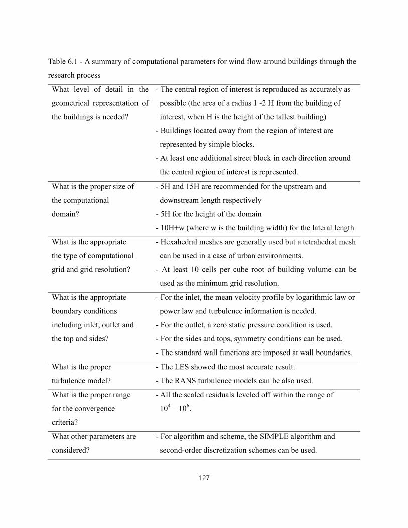
Table 6.1 - A summary of computational parameters for wind flow around buildings through the

research process

What level of detail in the

geometrical representation of

the buildings is needed?

- The central region of interest is reproduced as accurately as

possible (the area of a radius 1 -2 H from the building of

interest, when H is the height of the tallest building)

- Buildings located away from the region of interest are

represented by simple blocks.

- At least one additional street block in each direction around

the central region of interest is represented.

What is the proper size of

the computational

domain?

- 5H and 15H are recommended for the upstream and

downstream length respectively

- 5H for the height of the domain

- 10H+w (where w is the building width) for the lateral length

What is the appropriate

the type of computational

grid and grid resolution?

- Hexahedral meshes are generally used but a tetrahedral mesh

can be used in a case of urban environments.

- At least 10 cells per cube root of building volume can be

used as the minimum grid resolution.

What is the appropriate

boundary conditions

including inlet, outlet and

the top and sides?

- For the inlet, the mean velocity profile by logarithmic law or

power law and turbulence information is needed.

- For the outlet, a zero static pressure condition is used.

- For the sides and tops, symmetry conditions can be used.

- The standard wall functions are imposed at wall boundaries.

What is the proper

turbulence model?

- The LES showed the most accurate result.

- The RANS turbulence models can be also used.

What is the proper range

for the convergence

criteria?

- All the scaled residuals leveled off within the range of

104 – 106.

What other parameters are

considered?

- For algorithm and scheme, the SIMPLE algorithm and

second-order discretization schemes can be used.

7. IMMERSIVE CASE STUDY

7.1. Introduction

Generally, wind flow around buildings creates both negative and positive fluctuations over a

roofing system and these pressures are dynamic. In addition, the pressures can be separated into

static and fluctuating components. Due to vortex flow and separations, the wind pressure

distribution varies spatially over a roof and it can cause high suction at the corner and perimeter.

These high intermittent suctions could make the roofs susceptible to uplift and detachment. Thus,

the roof design must account for these situations that could occur from high winds (Baskaran et

al., 2007).

In an effort to resist wind fluctuation that can cause roof uplift failures, the roof vent system was

developed by Dr. Demetri Telionis, Dr. Jim Jones and Dr. Elizabeth Grant of Virginia Tech and

marketed by Acrylife®. For this roof vent system, it can eliminate the pressure variation that

causes the upward suction during high wind conditions creating a negative pressure zone

underneath the roof membrane. In addition, the performance of the roof vent system is highly

affected by its position. (Dockins & Tankersley, 2009). In order to determine layout of the roof

vent system, it is important to understand pressure and velocity on the roof surface.

Figure 7.1- Prototype of the roof vent system (Grant, 2003, p. 35)

The case studies reported in this chapter investigated the effect of design parameters such as

building height, aspect ratio and parapet height on the wind flow over the roof of a low-rise

building. While wind flow over the roof of a low-rise building has been generally tested using

wind tunnel testing and it provides reliable results, the cost is relatively high when compared to

numerical simulations and the number of parameters that can be tested is limited. In this study,

CFD was employed to investigate the effects of several different building configurations in order

to inform the design of low-rise buildings and to provide information such as the length of the

wind reattachment for roof vent systems.

Based on best practice guidelines, an analysis of journal articles and the sensitivity analysis, a set

of computational parameters were chosen for this study of wind flow around buildings. For the

case study, these computational parameters were reselected for the investigation of wind flow

over the roof because detailed information on both velocities and pressures are needed. All case

studies were designed to respond to the design parameters, specifically building height, building

aspect ratio, and parapet heights. In describing the scope of each case, the researcher immersed

himself into each case study and observed the entire CFD modeling process for wind flow over

the roof of a low-rise building.

7.2. Preparation for input computational parameters

As mentioned in Chapter 1, CFD simulation is a powerful tool in the development of building

design. However the simulation process is still very challenging. Thus, it is important to select

the right simulation models carefully. Moreover, the computational parameters should be

assessed iteratively in order to achieve the maximum results. This section presented preparation

for the selection of the computational conditions for case studies.

7.2.1. The selection of the turbulence model

During CFD processes, one of the most important steps is to select the proper turbulence model.

As mentioned in Chapter 6, the turbulence models based on the RANS approach can be generally

applied to the prediction of wind flow around building and the LES model can provide more

accurate result than the RANS turbulence models.

For the case study, the impact of design parameters such as building height, aspect ratio and

parapet height was investigated in order to provide information for the proper layout of the roof

vent systems. While the turbulence models based on the RANS approach provide easier

approach, their results provide overestimated wind flow on the roof. In order to compare the

differences between the LES model and the turbulence model based on the RANS approach,

these two turbulence models were applied to a building with height 36 ft, aspect ratio 1:2 and

parapet wall height 42 inch. Figure 7.2 showed the result of contours and vectors of the mean

velocity magnitude for the middle vertical plane of a building when the turbulence model based

on the RANS approach was applied. As mentioned in Chapter 6, the turbulence model based on

the RANS approach cannot reproduce the wind flow near the edge. Thus, the LES model was

recommended for this case study.

Figure 7.2 - The result of contours and vectors of the mean velocity magnitude for the middle

vertical plane of a building when the RANS turbulence model was applied

7.2.2. The selection of the geometry

For the geometry, two different roof surface areas were suggested: 50,000 ft2 and 150,000 ft2.

These two roof surface areas with a low rise building with height 36 ft, aspect ratio 1:2 and

parapet wall height 42 inch were applied into the computational domain using the

recommendations described in Chapter 6. The grid for these two models consisted of hexahedral

meshes with a grid resolution of 723,580 cells for the roof surface area 50,000 ft2 and 1,870,000

cells for the others. As described in Section 6.5, as the number of cells increases, the cost of high

computing resources are required. For calculating time, approximately 350 hours were required

for the case with the roof surface area 50,000 ft2. In the other case with the roof surface area

150,000 ft2, the calculation took approximately 500 hours but the result was not sufficiently

accurate. As shown in Figure 7.3, the result of the roof surface area 150,000 ft2 showed that the

wind flow in flow direction was not fully calculated. Considering the computer resources and

run-time of the simulation, the geometry of the roof surface area 50,000 ft2 was applied for the

case study.

Figure 7.3 - The result of contours and vectors of the mean velocity magnitude for the middle

vertical plane of a building with the roof surface area 150,000 ft2

7.2.3. Other computational parameters

Other computational parameters such as boundary conditions utilized the benchmark data

provided by the wind tunnel tests at the IBHS (Chapter 5) and the sensitivity analysis (Chapter 6).

For example, the velocity profile for the inlet boundary condition was specified using power law

with an exponent of 0.143, which corresponds to an open land surface. In addition, the wind

speed was 60 mph which was the same conditions as the wind tunnel testing at the IBHS. For

case studie, a wind angle of 0 degrees was considered because of the large cost of the required

LES model. Once cases with the wind angle of 0 degrees are completed, the various wind angles

of 30 degrees, 45 degrees, 60 degrees will be tested for further research.

7.3. Case study A: An investigation of wind flow over a flat roof for two different building

heights

7.3.1. Introduction and context

For this case study, wind flow over the roof of a low-rise building with two different building

heights was investigated. As shown in Figure 7.4, the reference building with a height of 36 ft

and the other building with a height of 12 ft were created. For both buildings, the flat roof

surface area was 50,000 ft2 and the building aspect ratio which is the ratio of width to length was

1:2. In addition, a parapet wall with a height of 42 inch was considered for both buildings. A

wind speed of 60 mph was used for the inflow condition in the CFD simulations.

a. Reference model: Height=36 ft b. Building with height=12 ft

Figure 7.4 - Two different building height


For this case study, two computational domains were created using the recommendations

obtained through the research. The dimensions of the two computational domains are described

in Figure 7.5. For the reference model, the domain dimensions were L × W × H – 880 ft × 676 ft

× 180 ft and the blockage ratio was 9%. The computational domain size for the other building

with the height 12 ft was L × W × H – 636 ft × 676 ft × 60 ft. For this building, the ratio of the

lateral extension of the computational domain to its height was assumed to be similar to the

corresponding ratio of the building because the lateral direction was much larger than the height

(Franke et al., 2007).

a. Reference model (building height: 36 ft)

b. The 12 ft high building

Figure 7.5 - The two different computational domains


The grid for these two cases consisted solely of hexahedral meshes, as shown in Figure 7.6.

Since significant information regarding the details of turbulent flow over the roof surface is

needed, hexahedral grids were employed. For the gird resolution, the base size of the grid was

based on the smallest length scale of the building. For both models, the base size for grid

generation was based on the parapet wall height. As described in Section 6.5, coarser and finer

grids were constructed. However, more than 1,000,000 grids required considerably higher

computing resources (See Section 7.2). Thus, a grid resolution of 723,580 cells for the reference

model and 842,940 cells for the other was selected.

a. Computational grids for the reference model

b. Computational grids for the 12 ft high building

Figure 7.6 - The computational grids


As mentioned previously, the experimental data should be specified for the inlet boundary

conditions. However, the measurement data was not available for this case study so the inlet

velocity profile was defined using the power law with an exponent of 0.143, which corresponds

to an open land surface. The velocity at a height of 33 ft was 60 mph.

For other boundary conditions such as the top, sides and outlet condition, the same boundary

conditions as those used in Chapter 6 were applied because the simulation settings of the case

study was similar to those of CFD modeling in Chapter 6. Symmetry boundary conditions were

applied for the sides and the top of the computational domain. For the outlet condition, a static

pressure of zero was defined. Within the computational domain, no-slip wall boundary

conditions were applied for the surfaces of the building.



RANS equations. The LES model was used for this analysis because it offers a useful way to

predict wind flow distributions over the roof surface. As described in Chapter 6, the same

conditions for the LES model were applied. The SIMPLE algorithm with a central differencing

scheme was employed. In order to calculate the subgrid scale in the LES model, the Dynamic

Smagorinsky Subgrid Scale model was used. The LES calculations were initialized with the

solution from the standard k-ɛ simulations. For the initial conditions, the steady state calculation

was first performed using the standard k-ɛ model. Once sufficient convergence was obtained, the

turbulence model was changed to the LES model and the unsteady calculation started

(Kobayashi et al., 2013). For this study, the time interval was 2.0 × 10-4 s, calculated for 50,000

time steps in total. When all the scaled residuals reached a minimum of 105, convergence for the

LES model was obtained.



First, the results of the computations in terms of velocity were analyzed for two cases. Figure 7.7

shows a comparison of the predicted mean velocity magnitude for the middle vertical plane and

on the roof surface. According to this comparative view of the results, the wind flow patterns in

the two cases are similar. For the reference model, the upwind flow near the edge is stronger and

the length of the wind reattachment is shorter than for the other case.

a. The reference model b. The 12 ft high building

Figure 7.7 - Contours and vectors of mean velocity magnitude on the roof and for the middle

vertical plane

a. The reference model b. The 12 ft high building

Figure 7.8 - Contours of pressure coefficients on the roof

Figure 7.8 shows the contours of the pressure coefficient distribution on the roof surface for each

case. Similar to the comparisons in Figure 7.7, the results for the reference model predict lower

pressure coefficients near the edge than for the other case.

7.3.6.2. Comparisons of pressure coefficient distributions on the roof surfaces

As shown in Figure 7.9, the CFD results for the reference model were compared with the results

for the building with a height of 12ft. For both cases, high suction values were observed near the

edge, decreasing rapidly as it progressed along the centerline. While the highest suction for the

reference model was observed 62 ft in from the edge, the suction for the other case was highest

32 ft from the edge. Both Cp values were the same at the middle of the roof surface. These

results clearly indicate that differences in building height influenced the wind flow over the roof

surface.

Figure 7.9 - CFD simulation results for the pressure coefficient along the centerline of the roof

surface for the two structures

7.3.7. Discussion

This case study focused on investigating CFD simulations of wind flow over a roof surface and

the impact of different building heights. The study’s discussions for the CFD process can be

summarized as follows.

1) For the size of the computational domain, while the computational domain for the reference

model was constructed using the recommendations obtained through Chapter 3 to 6, the

computational domain for the building with the height 12 ft was created using best practice

guidelines (Franke et al., 2007). For this case, it was difficult to generate the wind profile

using the same recommendations as those used for the reference model because the lateral

Cp

X/H

X

H

The reference model

12 ft building

direction was much larger than the height of the building. Thus, the ratio of the lateral

extension of the computational domain to its height was assumed to be similar to the

corresponding ratio of the building in order for the sufficient distance for the wind profile at

the inlet.

2) For the grid generation, the same base size of the grid was applied for both cases. Based on

the base size, the coarser and finer grids were constructed. In the case of the coarse grid, it

caused computational errors in representing the parapet wall. While the fine grids represented

the parapet wall, more than 1,000,000 grids were generated. Thus, a grid resolution of 723,580

cells for the reference model and 842,940 cells for the other were applied for this case study.

7.4. Case Study B: A comparisons of wind flow over a flat roof surface with two different

building aspect ratios


For the second case study, the wind flow over the flat roofs of two low-rise buildings with

different building aspect ratios was investigated. As shown in Figure 7.10, two different building

aspect ratios were created: 1:2 for the reference building and 1:1 for the other. For both buildings,

the roof surface area was 50,000 ft2 and the building height was 36 ft. A parapet wall with a

height of 42 inch was used for both cases. 60 mph was used for the inflow condition in the CFD

simulations.

a. Reference model: Aspect ratio 1:2 b. Test building: aspect ratio 1:1

Figure 7.10 - Two different building aspect ratios


For this case study, two computational domains were created. The dimensions of these

computational domains were as described in Figure 7.11. For the reference model, the same

computational domain as that used in the first case study was applied. The computational domain

size for the other building with the building aspect ratio 1:1 was L × W × H – 944 ft × 584 ft ×

180 ft.

a. Reference model with the building aspect ratio 1:2

b. Test building with the building aspect ratio 1:1

Figure 7.11 - Two different computational domain


As described in the first case study in Section 7.3.3, the grid for these two cases consisted solely

of hexahedral meshes, as shown in Figure 7.12. For the grid resolution, 723,580 cells were

generated for the reference model. For the building with the aspect ratio 1:1, the grid consisted of

687,430 cells.

a. Computational grids for the reference model with a building aspect ratio 1:2

b. Computational grids for the building with a building aspect ratio 1:1

Figure 7.12 - The computational grids


As described in the first case study in Section 7.3, the velocity profile was specified at the inlet

boundary condition using a power law with an exponent of 0.143, which corresponds to an open

land surface. The velocity 33 ft above the ground was 60 mph. For the sides and the top of the

computational domain, symmetrical boundary conditions were applied. For the outlet condition,

a static pressure of zero was defined. Within the computational domain, no-slip wall boundary

conditions were applied for the surfaces of the building in the computational domain.



RANS equations. The LES model was used for this analysis because it offers a useful way to

predict wind flow distributions over a flat roof surface. In addition, the SIMPLE algorithm with a

central differencing scheme was employed. In order to calculate the subgrid scale in the LES

model, the Dynamic Smagorinsky Subgrid Scale model was used.

The LES calculations were initialized with the solution from the standard k-ɛ simulations. For

the initial conditions, the steady state calculation was first performed using the standard k-ɛ

model. Once sufficient convergence was obtained, the turbulence model was changed to the LES

model and the unsteady calculation started (Kobayashi et al., 2013). For this study, the time

interval was 2.0 × 10-4 s, calculated for 50,000 time steps in total. When all the scaled residuals

reached a minimum of 105, convergence for the LES model was obtained.


7.4.6.1. Qualitative comparisons

Contours and vectors of the mean velocity magnitude for both cases are compared in Figure 7.13.

This comparative view of the results clearly shows the differences in the velocity field behavior

for the two cases. In this case, the wind flow patterns were similar and a large difference was not

observed.

a. The reference model: Aspect ratio 1:2 b. The building with aspect ratio 1:1

Figure 7.13 - Contours and vectors of mean velocity magnitude on the roof and for the middle

vertical plane

Figure 7.14 presents the contours of the pressure coefficients on the roof surface. As for the

comparison of mean velocity magnitude, the results for both cases revealed similar trends,

although somewhat lower values in pressure coefficients for the reference model were observed

near the edge.

a. The reference model b. Test building with a height of 12 ft

Figure 7.14 - Contours of pressure coefficients on the roof

7.4.6.2. Comparison of the pressure coefficient distributions on the roof surfaces for the

three grids

Figure 7.15 compares the pressure coefficient distribution along the centerline of the roof surface

obtained from CFD for both cases. Near the edge, the pressure coefficient in the reference model

was somewhat lower than for the other case. The highest suction was observed at 62 ft and 20 ft

from the edge for the reference building and the other building, respectively.

Figure 7.15 - Results of pressure coefficients along the centerline of the roof surface

7.4.7. Discussion

This case study focused on an analysis of wind flow over the flat roof surface of a low-rise

building with two different building aspect ratios.

For the CFD process, the size of the computational domain for the model with building aspect

ratio 1:1 was created using the recommendations in Chapter 6. In addition, the same base size of

the grid as used for the reference model was applied for this model. For boundary conditions, the

same conditions used for the sensitivity analysis (Chapter 6) were applied because the geometry

and the simulation settings were similar.

Cp

X/H

X

H

The reference model

The building aspect ratio 1:1

7.5. Case Study C: A comparisons of wind flow over the flat roof surface of a low-rise

building with three different parapet walls


For this case study, wind flow over the flat roof of a low-rise building with three different

parapet walls was investigated. As shown in Figure 7.16, three different parapet walls were

defined. For these parapet walls, heights of curb edge (3 inch), 24 inch and 42 inch were applied

to the reference building. The building height and aspect ratio used for the reference building in

the first and second case studies, respectively, was applied. A wind speed of 60 mph was used for

the inflow condition in the CFD simulations.

Figure 7.16 - The reference building with three different parapet walls


For this study, the same computational domain used for the reference model in the first and

second case studies was applied. The dimensions were L × W × H – 880 ft × 676 ft × 180 ft and

the blockage ratio was 9%. This is shown in Figure 7.17.

Figure 7.17 - The computational domain for the reference model


For this case study, three grids were generated using hexahedral meshes. As shown in Figure

7.18, 723,580 cells were generated for the reference model with a 42 inch parapet wall, the

building with a 24 inch parapet wall utilized 791,250 cells, and 833,920 cells were generated for

the building with a 3 inch curb edge.


As described in the first and second case study, the velocity profile was specified at the inlet

boundary condition using a power law with an exponent of 0.143, which corresponds to an open

land surface. The velocity 33 ft above the ground was 60 mph.

For the sides and the top of the computational domain, symmetrical boundary conditions were

applied. For the outlet condition, a static pressure of zero was defined. Within the computational

domain, no-slip wall boundary conditions were applied for the surfaces of the building in the

computational domain.

a. Computational grids for the reference building with the 3 inch curb edge

b. Computational grids for the reference building with 24 inch parapet wall

c. Computational grids for the building with 42 inch parapet wall

Figure 7.18 - The computational grids for the three different parapet walls



RANS equations. The LES model was used for this analysis because it is a good way to predict

wind flow distributions over a flat roof surface. In addition, the SIMPLE algorithm with a central

differencing scheme was employed. In order to calculate the subgrid scale in the LES model, the

Dynamic Smagorinsky Subgrid Scale model was used.

The LES calculations were initialized with the solution from the standard k-ɛ simulations. For

the initial conditions, the steady state calculation was first performed using the standard k-ɛ

model. Once sufficient convergence was obtained, the turbulence model was changed to the LES

model and the unsteady calculation started (Kobayashi et al., 2013). For this study, the time

interval was 2.0 × 10-4 s, calculated for 50,000 time steps in total. When all the scaled residuals

reached a minimum of 105, convergence for the LES model was obtained.


7.5.6.1. Qualitative comparisons

In Figure 7.19, the mean velocity magnitudes of vertical cross-section for each turbulence model

are presented. The wind flow patterns for three cases were similar but the wind reattachment

region migrated closer to the edge as the parapet wall height diminished.

a. The reference model with the parapet height 42 inch

b. The building with the parapet height 24 inch

c. The building with the curb edge

Figure 7.19 - Contours and vectors of mean velocity magnitude on the roof and for the middle vertical plane

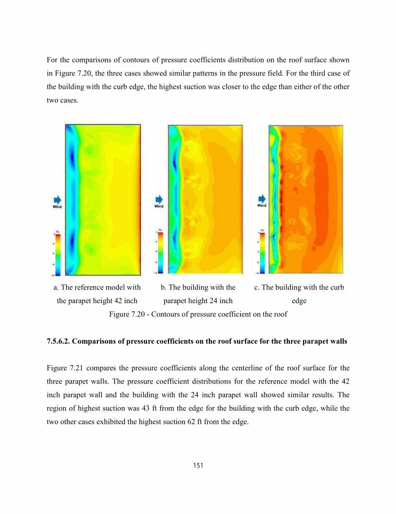
For the comparisons of contours of pressure coefficients distribution on the roof surface shown

in Figure 7.20, the three cases showed similar patterns in the pressure field. For the third case of

the building with the curb edge, the highest suction was closer to the edge than either of the other

two cases.

a. The reference model with

the parapet height 42 inch

b. The building with the

parapet height 24 inch

c. The building with the curb

edge

Figure 7.20 - Contours of pressure coefficient on the roof

7.5.6.2. Comparisons of pressure coefficients on the roof surface for the three parapet walls

Figure 7.21 compares the pressure coefficients along the centerline of the roof surface for the

three parapet walls. The pressure coefficient distributions for the reference model with the 42

inch parapet wall and the building with the 24 inch parapet wall showed similar results. The

region of highest suction was 43 ft from the edge for the building with the curb edge, while the

two other cases exhibited the highest suction 62 ft from the edge.

Figure 7.21 - CFD simulation results: Impact of turbulence models on the pressure coefficients

along the centerline of the roof surface

7.5.7. Discussion

CFD simulations for the wind flow around a building with three different parapet wall heights

were compared. The parapet wall heights tested were: curb edge (3 inch), 24 inch and 42 inch.

The discussions for the CFD process are summarized as follows.

1) For the third case study, the same computational domain was used for the three cases. Only

three different parapet wall heights were considered.

2) During the CFD process, the grid generation was a very time consuming because of the large

difference in length scale between the parapet heights and the computational domain. As

Cp

X/H

X

H

Reference model: 42 inchParapet wall: Curb edge

Parapet wall height: 24 inch

mentioned above, very large discretization errors were occurred when representing two small

parapet wall heights of the curb edge (3 inch) and 24 inch. Thus, the different base size of the

grid was applied for the two cases in order to avoid the computational errors.

7.6. Summary of case studies

The three case studies described above investigated the impact of different building

configurations including the building height, aspect ratio and parapet wall heights. The CFD

modeling conducted for each case study employed the computational parameters identified

through the document analysis and the sensitivity analysis reported in Chapters 3 to 6. The

findings of the three case studies can be summarized as follows:

1) Wind flow over the flat roof surface of a low-rise building for three different building

configurations was examined using CFD simulations and the mean velocity magnitude and

pressure coefficient distributions calculated. Among these building configurations, the

building height significantly influenced wind flow over the roof surface. As the building

height increases, lower values of the pressure coefficient can be achieved.

2) The parapet wall also affected the wind flow behavior over the roof surface. Wind flow and

pressure field were not highly influenced by increasing the height of the parapet wall between

the heights 24 inch and 42 inch. However, the comparison between the curb edge and the other

parapet walls showed a significant difference in the pressure coefficients near the edge. As the

parapet wall height decreased, the region of wind reattachment migrated closer to the edge.

3) While somewhat lower values of pressure coefficients were observed for the reference model,

the building aspect ratio did not substantially influence wind flow over the roof surface.

7.7. Discussion of the computational parameters through case studies

For the case studies, CFD simulations were employed to investigate the wind flow behaviors

over the flat roof surface of a low-rise building for several building configurations.

Computational parameters for wind flow around buildings were obtained through document

analysis and sensitivity analysis. However, several parameters such as turbulence model and grid

type were reselected to better reproduce the wind flow over the building.

In order to represent the wind flow behaviors on the roof surface, the LES model was applied. As

mentioned in Chapters 3 to 6, this turbulence model requires substantial calculating time and

computational resources. Since the k-ε turbulence models based on the RANS equations cannot

adequately represent wind flow over a roof surface, the LES model was used for this case study.

For calculating time, approximately 350 hours were required to achieve the results presented

here.

For the grid type, a hexahedral grid was used rather than a tetrahedral grid because of its

convenience for achieving numerical values and improving accuracy. Although a tetrahedral grid

is generally preferred to represent the air flow patterns around buildings in urban areas, it is

difficult to plot the resulting numerical data. For this case study, it was necessary to compare

numerical values such as pressure coefficients in order to examine the impact of several building

configurations. Thus, a hexahedral grid was employed.

The other computational parameters, including the computational size, grid resolution, boundary

conditions, and convergence criteria, were obtained using the procedures described in Chapters 3

to 6 for this case study.

8. CFD AS A DESIGN ASSITANCE TOOL IN SCHEMATIC DESIGN STAGE

Computational parameters were analyzed and specified for wind flow around buildings through

the research process. Based on the results, the CFD process for specific computational

parameters was obtained. This chapter presents the findings of this study based on a sensitivity

analysis and supported by the reviewed documents. The findings will now be considered in terms

of the two themes that emerged from the data:

1) Which computational parameters maximize the accuracy of the CFD modeling? and,

2) Which computational parameters facilitate the effective use of CFD as a design assistance tool

regarding time efficiency and ease of use?

Considering the above two themes, the data presented in the following sections focus on the

researcher’s observations regarding collecting and analyzing data related to the computational

parameters in the context of CFD simulations of wind flow around a building. Within the CFD

process, the pre-processing steps that consist of selecting the commercial code, preparation of

geometry, the size of computational domain, grid generation, selecting boundary condition and

turbulence model were the primary considerations.

8.1. Selecting the commercial code

Many commercial codes have been employed to simulate flow problems. Among these, the code

FLUENT has been most widely applied; all the journal articles in Chapter 5 used FLUENT for

their studies, for example. As mentioned in Chapter 2, FLUENT has three major components: 1)

GAMBIT (the mesh generator), 2) FLUENT Solvers and 3) the FLUENT post-processor

(ANSYS FLUENT, 12.0). In the case of the code STAR-CCM+, it provides a single integrated

software environment from CAD creation to post-processing that automates simulation workflow

and performs iterative design studies with minimal user interaction. In addition, the CAD-

embedded environment of STAR-CCM+ does not require detailed knowledge of a specialist

simulation package (http://www.cd-adapco.com/products/ comprehensive-simulations).

Although FLUENT has been widely used and its accuracy and reliability has been verified, it

does suffer from difficulties when creating models and meshes from other tools. Moreover, the

user-friendly interface and a single integrated environment of STAR-CCM+ provide an easier

approach to solving time consuming tasks such as repeated simulations on design variables for

designers and analysts than those offered by FLUENT. The accuracy and credibility of STAR-

CCM+ have been confirmed by a number of recent publications (Lo et al, 2013; Pieterse &

Harms, 2013; Norton et al., 2010; Zeng et al., 2012).

In addition, STAR-CCM+ was used for the sensitivity analysis and the case studies for this study.

As mentioned above, this approach reduced the time required for repeated CFD simulations such

as those utilized for these analyses.

Table 8.1 shows a comparison of the characteristics of the two commercial codes. Considering

the advantages and disadvantages of both, the code STAR-CCM+ is recommended for predicting

wind flow around buildings in the architectural design process.

Table 8.1 - Comparison between the characteristics of FLUENT and STAR-CCM+

CFD Code Accuracy Effective use of CFD

Time efficiency Ease of use

FLUENT ✓

STAR-CCM+ ✓ ✓ ✓

8.2. Preparing the geometry

One of the most difficult and time consuming processes is the preparation of the geometry. As

mentioned in Chapter 4, the area of a radius 1-2 H from the building of interest must be

reproduced as accurately as possible, where H is the height of the tallest building in the region of

interest. In addition, at least one additional street block in each direction around the region of

interest must also be clearly reproduced, with buildings located away from the central region

being represented by simple blocks. For example, Hooff & Blocken (2010) investigated urban

wind flow and natural ventilation for the Amsterdam ArenA stadium using CFD techniques. As

indicated in Figures 8.1 and 8.2, they modeled the ArenA stadium in great detail but the

buildings situated within a radius of 500 m from the stadium were reproduced by only their main

shape.

Figure 8.1 - Aerial view of the area north of the Amsterdam ArenA football stadium and its

surroundings (Hooff & Blocken, 2010)

Figure 8.2 - Grid generation for the Amsterdam ArenA football stadium and surroundings:

(a) Computational model geometry, view from northeast; (b) computational grid for the

building surfaces and part of the ground surface (Hooff & Blocken, 2010)

8.3. The computational domain size

Once the geometry has been cleaned up and represented, it is transferred into the computational

domain. Generally a rectangular computational domain is used in urban-scale studies in which

wind is simulated with a constant profile, entering from upstream, encountering buildings of

interest, and exiting the domain downstream (Gousseau et al., 2011; Mirzaei, & Carmeliet, 2012;

Tominaga & Stathopoulos, 2011). Depending on the wind flow analysis through wind rose and

Climate Consultant, the inflow direction of the computational domain is determined and the

magnitude of the approaching wind is simplified according to the existing prevailing and

frequent winds on the area of interest (Mirzaei, & Carmeliet, 2012). For example, the wind

statistics for the location of the Eindhoven university campus were illustrated by means of wind

rose in Figure 8.3. This wind rose was divided into twelve directions with frequency distribution

of the hourly mean wind speed. According to the wind analysis through the wind rose, twelve

different computational domains have to be created in order to cover twelve different wind

directions. However, this would be an idealistic assumption because it is not easy to consider all

approaching winds in the architectural design process. Thus, the wind from one or two prevailing

directions obtained through wind rose or Climate Consultant can be used to determine the inflow

direction in the computational domain. However, if no one or two wind directions are dominant

form the wind rose analysis, then a decision must be made concerning multiple analyses for a

range of wind directions and simulation domain orientations.

Figure 8.3 – Standard wind rose with frequency distribution of the hourly mean wind speed for

Eindhoven University campus (Janssen et al., 2013)

Through the inflow direction of the computational domain, 5H and 15H are used for the

upstream and downstream length respectively, where H is the height of the tallest building. In

addition, 5H is used for the vertical extension and 10H+w is used for the lateral extension, where

w is the built area that surrounds the region of interest. Figures 8.3 and 8.4 show examples

representing the computational domain of a single building and its urban environment,

respectively. In Figure 8.3, a single building tested at the wind tunnel at the IBHS is represented

in the computational domain, applying 5H for the upstream length and 15H for the downstream

length. The height and width of the wind tunnel were used for the lateral and vertical domain

lengths. In Figure 8.4, the park tower and its urban surroundings in Antwerp are represented in

the computational domain. Here, the computational domain consists of the basic domain and an

additional downstream subdomain for wind directions 180°–270° because the prevailing wind

direction is 210°. The explicitly modeled buildings are the park tower and the surrounding

buildings for a rectangle of 1037 by 632 m2 around the tower, when the height of the park tower

is 78.18 m. The tower is reproduced in detail, while the surrounding buildings are represented by

only their main shape (Montazeri et al. 2013). For this computational domain, the distance from

the building to the side, to the inlet and to the top of the domain is at least five times the height of

the building and the distance from the building to the outlet is fifteen times the height.

As can be seen in Figures 8.4 and 8.5, these are consistent with best practice guidelines.

Therefore, the size of the computational domain recommended by best practice guidelines can be

employed.

a. Test building in the wind tunnel at the IBHS

b. Layout of the test building and the chamber

c. The test building in the computational domain

Figure 8.4 - A single building in the computational domain

a. Aerial view of the Park Tower (red) and surrounding buildings

b. Top view of Park Tower and wider surroundings in a rectangular area of 630–1000 m2 with

an indication of building heights

c. Computational domain for wind directions 180°–270°, consisting of a basic domain and an

additional downstream domain

Figure 8.5 - The computational domain of an urban area in Antwerp (Montazeri et al. 2013)

8.4. Grid generation

Once the computational domain size has been determined, this domain must be discretized using

grids that provided an adequate resolution of the geometry and expected flow fields (Casey &

Wintergerste, 2000). Two types of grid topologies are generally used to capture the geometrical

details of domains: structured grids and unstructured grids. For structured grids, the connectivity

is straight-forward and employs a hexahedral shape. In the case of unstructured grids, a

tetrahedral shape is utilized. According to Franke et al. (2007), hexahedral grids are to be

preferred as they lead to smaller truncation errors and better iterative convergence than

tetrahedral grids. However, a tetrahedral mesh generally provides a better fit for complicated

domains and offers more convenient mesh adaptivity (Oliveira et al., 2008). According to a study

by Hefny & Ooka (2009), generating hexahedral grids follows the structured grid constraint of

having continuous gridlines on all faces, which requires the domain to be subdivided into blocks.

Since the gridlines must remain continuous throughout the geometry, these blocks are difficult to

develop. By contrast, tetrahedral grids can be generated automatically using commercial grid

generation software packages (Hefny & Ooka 2009). When it comes to accuracy, it is commonly

accepted that hexahedral grids provide more accurate results than tetrahedral grids at similar

densities. Tetrahedral grids also require 4–10 times more elements than a hexahedral grid to

obtain the same level of accuracy (Hefny & Ooka 2009; Shepherd & Johnson, 2007).

Table 8.2 - Comparison between the characteristics of hexahedral and tetrahedral grids

Grid type Accuracy Effective use of CFD


Hexahedral grids ✓

Tetrahedral grids ✓

Table 8.2 shows a comparison of the characteristics of the two types of grids. As described above,

it is normally recommended that hexahedral grids be used for accuracy. For example, a

hexahedral grid was used for the sensitivity analysis in Chapter 6. The geometry of the test

building in the wind tunnel test at the IBHS consists of a simple block. For this geometry, a

hexahedral grid was used and the detailed information of velocities or pressures was easily

achieved for the analysis. However, it is often difficult to reproduce urban flow situations using

hexahedral grids, while tetrahedral grids are created automatically by the software. Hexahedral

grids may also cause computational errors during grid generation. When considering time

efficiency, correcting the computational errors created by hexahedral grids may take longer than

the computational resources required when using tetrahedral grids to achieve the same level of

accuracy. Thus, hexahedral grids are preferred for a simple geometry such as wind tunnel testing,

while tetrahedral grids are preferred for the representation of urban wind flows regarding the

time efficiency.

Considering the aspects of ease of use and time efficiency, it is thus recommended that a

tetrahedral grid be used for the representation of urban wind flow situations. However, a

hexahedral grid can be used for a simple geometry such as wind tunnel testing and when highly

detailed information is required.

8.5. Turbulence model

Of the many ways of treating turbulent flows, the RANS equations have been most widely used

for CFD simulations of industrial flows. These equations are derived by time or ensemble

averaging the Navier-Stokes equations, reducing the resolution requirements by many orders of

magnitude. However, because of the averaging procedure involved, information about the

turbulence is lost. In the RANS equations, many different turbulence closures have been

provided, including different versions such as the k-ε model, the k-ω model, and so on. These

two-equation models are the mainstay of CFD simulations and provide a good compromise

between complexity, accuracy and robustness. In order to achieve significant information

regarding the details of turbulent flow, LES methods can be used that are based on the numerical

resolution of the large turbulence scales and the modeling of the small scales. Due to the large

cost of the required unsteady simulations, this approach is not employed routinely in industrial

flow simulations (Menter et al., 2002), although as computer technology continues to develop,

the use of the LES approach is becoming feasible and it is now beginning to be used to analyze

industrial flow.

According to the journal articles related to the representation of urban wind flow discussed in

Chapter 4, the RANS approach with the realizable k-ε model, the RNG k-ε model and standard

k-ε model have been most popular because they are easier to use than the LES model and less

time consuming. Considering the results of the sensitivity analysis for the turbulence model

presented in Chapter 6, the RANS approaches generally took 6 to 8 hours to achieve

convergence, while the LES took 40 times longer than either of the RANS models to do so.

Table 8.3 - Comparison of the characteristics of the RANS approach and the LES model

Turbulence model Accuracy Effective use of CFD


The RANS approach ✓ ✓

LES model ✓

Table 8.3 compares the RANS approach and the LES model. In the architectural design process,

CFD has been generally used to modify design problems related to air flow in and around

buildings. For this process, it is difficult to use the LES model because it requires more

computational resources and time than those needed for the RANS turbulence model. Also,

additional computational parameters such as time step and time interval must be set for the LES

model.

Considering time efficiency and ease of use, RANS approaches such as the realizable k-ε model

are recommended for studying wind flow around buildings in the architectural design process. In

the case of the LES model, it can be used for the accurate information of velocities and pressures

such as wind uplift on the roof surface (Chapter 6 and 7).

8.6. Boundary conditions

The boundary conditions reproduce the influence of the surroundings when cut off by the

computational domain (Franke et al., 2007). In general, it is difficult to define some of the

boundary conditions at the inlet and outlet of the computational domain at the level of detail that

is required for an accurate simulation (Casey & Wintergerste, 2000). Significant care is therefore

required when specifying the boundary conditions.

For the inlet boundary conditions, the data from experiments, including the turbulent kinetic

energy k and dissipation rate ɛ, are needed to prescribe the profiles. Most of the studies discussed

in Chapter 4 determined the velocity profile at the inlet using the measured wind profile from

experiments and it was specified using logarithmic or power laws. In the case of the use of CFD

in the architectural design process, the information pertaining to wind data and turbulence from

measurements are not generally available because a design concept at the schematic design stage

does not yet exist. In order to specify the mean velocity profile at the inlet, the information

obtained from previous studies related to similar issues or the weather condition at the site can be

used. When deciding between the use of a logarithmic law or a power law to create wind speed

profiles, the following equations apply. For a log law, the wind profile is given by:

U �z� � �∗� ��

�� Equation 8.1 – A log-law for the wind profile

where u* is the surface friction velocity, k is von Karman's constant (0.4), d is the zero plane

displacement and z0 is the surface roughness length (Drew et al., 2013).

In the case of a power law, the mean velocity profile is given by

U �z�� U��

Equation 8.2 – A power law for the mean velocity profile

where U(Z1) and U(Z2) are the mean wind speeds at heights of Z1 and Z2, respectively, and α is

the magnitude of the exponent (Drew et al., 2013). Values for the terrain dependent parameters

are typically those shown in Table 8.4. Using these equations, the mean wind profile can be

specified at the inlet boundary condition.

Table 8.4 - Values for typical terrain dependent parameters in the UK (Cook, 1997, as quoted in

Drew et al., 2013)

Description Typical rural Suburban City

Roughness length, Z0 (m) 0.03 0.3 0.8

ABL Height (m) 2550 3000 3250

Exponent α 0.16 0.24 0.32

For the outlet boundary conditions, zero static pressure can be imposed and symmetrical

boundary conditions employed for the top and sides of the domain.

8.7. Numerical schemes and the algorithm

In general, higher order approximations such as second-order methods are recommended for

dealing with this type of problem (Franke et al., 2007). For the RANS approach, the SIMPLE

algorithm is employed for pressure-velocity coupling, pressure interpolation is second order and

second-order discretization schemes are used for both the convection terms and the viscous terms

of the governing equations.

8.8. Convergence criterion

As Franke et al. (2007) explain, CFD simulations employ iterative methods to solve the algebraic

system of equations. The termination criterion is usually based on the residuals of the

corresponding equations and a typical termination criterion of 0.001 is used in industrial

applications. For example, one of the studies examined in Chapter 4 used termination criteria of

106 for the x, y and z momentum, and 105 for k, ɛ and continuity (Montazeri & Blocken, 2013)

and Abohela et al. (2013) also set their scaled residuals in the range of 104 – 106. Hence,

convergence is assumed to obtain when all scaled residuals are reached in the range of 104 – 106.

8.9. Conclusions regarding the CFD simulation process for wind flow around buildings in

the schematic design stage

Concerning the data gathered from the analysis of documents, the sensitivity analysis, and

observations, the optimal CFD modeling process for wind flow around buildings can be

summarized as follows:

8.9.1. Pre-processing

1) The commercial CFD code: STAR-CCM+

2) Prepare the geometry:

- The central region of interest (the area of a radius 1-2 H from the building of interest) is

reproduced as accurately as possible.

- One additional street block in each direction around the region of interest is also clearly

reproduced.

- Buildings located away from the region of interest are represented by simple blocks.

3) Transfer the AutoCAD file: Stereo lithography file (.stl), IGES (.iges and .igs), etc. of

AutoCAD file formats

4) The computational domain size:

- With H being the height of the building of interest, upstream and downstream lengths of 5H

and 15H, respectively

- 5H for the height of the domain

- 10H+W (the width of built area) for the lateral extension

5) Grid design:

- Tetrahedral grids

- At least 10 cells per cube roof of building volume for grid resolution

6) Turbulence model: the RANS equations with the realizable k-ɛ turbulence model

7) Boundary conditions:

- The inlet: the mean vertical velocity profile is specified using a power law or log law.

- The outlet: zero static pressure condition

- Top and sides of the domain: symmetry boundary conditions

8) Numerical schemes and the algorithm:

- The SIMPLE algorithm for pressure-velocity coupling, second order for pressure interpolation

and second-order discretization schemes are used in the RANS approach.

9) Convergence criterion: the scaled residuals were set in the range of 104 – 106.

8.9.2. Solving

1) The solution can be calculated using the solvers of STAR-CCM+ 8.04, with continuous

monitoring of the scaled residuals.

8.9.3. Post-processing

1) Visualization: the CFD results may conveniently be visualized as contour and vector plots of

velocity and pressure.

The computational parameters for wind flows around buildings can be presented via the CFD

process. Since the results of CFD simulations are very sensitive to a number of computational

parameters and these parameters are chosen by the user, a number of parameters were reviewed

and analyzed based on the findings of previous studies. Among the selected computational

parameters, conditions of the preparation of the geometry, the computational domain size, and

boundary conditions were developed using the recommendations. Other computational

parameters including turbulence models and grid generation were established through an analysis

of journal articles published since 2011, because the recent rapid developments in computing

power make it possible to incorporate more computational parameters. The selected

computational parameters can be used for the CFD analysis of wind flow around buildings. The

results of CFD will provide information regarding the air flow around building to architects and

designers to assist their design development in the schematic design stage.

9. LESSONS-LEARNED

9.1. Introduction

The research was designed to provide a better understanding of the CFD simulation process by

adopting a combined qualitative and quantitative approach. Through the case study research

method, the researcher described how the CFD modeling process can be conducted in the context

of wind flow around buildings in order to improve our understanding of the application of CFD

for building design.

By identifying computational parameters based on document analysis and observations during a

case study, lessons-learned were gathered. These lessons will be shared with others planning to

use CFD as a design assistance tool in order to help them use it more effectively and avoid

computational errors in the schematic design stage.

9.2. Consider influential factors in the urban area including vegetation and surface

characteristics when preparing the geometry

When commencing any project related to CFD, it is important to determine what must be

included and what can safely be ignored regarding the geometry of the target objects when

preparing the geometry. Generally the distribution of buildings is the major factor that influences

wind flow patterns, while secondary influencing factors in the urban area are vegetation and

surface characteristics such as roads, grass and sand (Franke et al., 2007).

In the case of CFD analysis for wind comfort, trees, grass, road and sand are generally neglected,

although vegetation has sometimes been considered in the planning process for the wind energy

industry. As the examples in Sections 8.2 and 8.3 demonstrate, surface characteristics are

generally not reproduced in the computational domain. Whether the details of the geometry are

included or excluded may significantly influence the number of grid cells. As noted earlier,

increasing the number of grid cells greatly increases the computing resources required and the

running time. The optimum balance to be struck is normally based on the user’s experience,

previous studies and the best practice guidelines.

9.3. Clean up and reproduce the initial design of the building of interest and surroundings

in the native AutoCAD file as much as possible before importing them into the

computational domain

After the appropriate level of detail in the geometrical representation has been determined, the

initial design of the building of interest and surroundings are reproduced and cleaned up in order

for them to be imported into the computational domain. Generally, the buildings in the native

AutoCAD file format are made of surfaces. When the AutoCAD file is imported into the

commercial CFD code, this may produce computational surface errors such as pierced faces, free

edges, non-manifold edges, etc. These computational surface errors may create substantial

computational volume errors which then go on to produce incorrect results in the CFD

simulation. In the case of the wind tunnel tests at the IBHS used for the sensitivity analysis

(Chapter 6), the test building in the wind tunnel was reproduced as solid object in the AutoCAD

and imported into the computational domain in order to avoid computational errors. Thus, it is

important to clean up and reproduce the initial design of the building of interest and its

surroundings in the AutoCAD file format. While the commercial CFD code provides a tool for

correcting computational errors, it is typically easier and faster for architects and designers to

clean up and reproduce them in the AutoCAD file format than to correct computational surface

errors in the commercial code. As mentioned above, the building of interest and its surroundings

should be represented as solid objects in order to be read into the commercial code.

9.4. Choose the proper grid type for various applications of building design

As mentioned in Section 8.4, it is important to choose the proper grid type associated with

various building design objectives including building site design, pedestrian wind comfort,

natural ventilation, pollutant dispersion around buildings, wind uplift on the roof, etc. Generally,

hexahedral grids are used for simple geometries, while tetrahedral grids are preferred for the

investigation of overall wind flow patterns in urban area and complex geometries. In order to

achieve results that satisfy a particular purpose, the grid type should be carefully selected.

A hexahedral grid is generally used to produce detailed information on velocity and pressure. For

natural ventilation as a design objective, a hexahedral grid is employed to calculate the air

exchange rate in a building and for the prediction of pollutant dispersion around buildings. A

hexahedral grid is used for the calculation of how the pollutant dispersion is influenced by

surrounding buildings. In addition, this type of grid can be used to produce detailed information

such as the velocity and pressure on the roof for the investigation of wind uplift. For example, a

hexahedral grid was used for both the sensitivity analysis in Chapter 6 and the case studies in

Chapter 8 because detailed information on turbulence quantities was required. While the

geometry of the wind tunnel tests in Chapter 5 consisted of a simple block, the geometry for the

case studies in Chapter 7 employed large differences in geometrical length scales between the

computational domain and the parapet wall. However, although it caused computational errors

when a hexahedral grid was applied for the geometries in Chapter 8, this grid was deemed to be

more useful overall because of its accuracy and convenience as a way of achieving numerical

values for velocities and pressures.

A tetrahedral grid is generally employed to inform the design of building site planning and wind

comfort studies because of its mesh adaptivity for complex geometries. For example, a

tetrahedral grid is generally used to predict the distributions of air velocity around buildings.

Table 9.1 summarizes the recommendations for the selection of the proper grid type in the light

of various building design objectives.

Table 9.1 - Recommendations for the selection of a suitable grid type for various applications

Building design Computational grids

Hexahedral grids Tetrahedral grids

A study of natural ventilation design ✓

Building site planning ✓

An assessment of pedestrian wind comfort ✓

Prediction of pollutant dispersion ✓

Investigation of wind uplift on the roof ✓

9.5. Consider the smallest length scale of the building of interest when determining the base

size of grids and check for computational errors after grid generation

The most time-consuming and difficult task in the CFD process is the grid generation. To achieve

accurate results, it is important to understand the influence of the mesh size. However, issues

concerning a suitable mesh density to achieve the desired accuracy for a specific problem still

remain. Although commercial CFD codes can automatically generate grids, it is important to

have proper initial values for the base grid size.

When generating grids, the base size should be set up as approximately 5% to 10% of the length

of the building of interest. Considering the smallest length scale of the building of interest, the

value for the base grid size can be varied in order to produce accurate results. In the case of the

sensitivity analysis in Chapter 6, the base size of grids was approximately 10% of the length of

the test building in the wind tunnel and the results of the computational model showed good

agreement with the finer grids. This comparison is shown in Figure 6.13. In addition, the

smallest length scale was focused on the parapet wall of the building in the case studies in

Chapter 7. After the grids have been generated, it is strongly recommended to check whether

computational errors are created at the building of interest.

9.6. Choose the proper turbulence model for applications of building design, namely either

LES or the RANS turbulence model

The selection of the turbulence model depends on considerations such as the physics

encompassed in the flow situation, the objectives for a specific problem, and the amount of time

available for the simulation. For the architectural design process, it is important to choose the

most appropriate turbulence model for various objectives of building design including the study

of natural ventilation, a prediction of pollutant dispersion around buildings, an assessment of

pedestrian wind comfort, building site planning and an investigation of wind uplift on the roof.

As mentioned in Chapter 6, the LES model provides more accurate information about turbulence

quantities such as velocity and pressures. In addition, the sensitivity analysis showed that LES

gave better results than either of the two RANS turbulence models at the perimeter of the roof

(Chapter 6). The LES model was therefore used for the investigation of wind uplift on the roof

surface described in Chapter 7 as it provided more detailed information regarding wind loads on

the roof. Moreover, the LES model when used for the prediction of the pollutant dispersion did

not underestimate the turbulence kinetic energy at the recirculation zone on the roof (Gousseau et

al., 2011) as the RANS models did. In the case of an investigation of roof detachment in

hurricane prone areas, the LES model would be more reliable.

Because the modeling process is easier and simulations take much less time, the RANS

turbulence models are generally employed for the study of natural ventilation, an assessment of

pedestrian wind comfort and building site planning.

Although LES can predict wind loads on the roof and pollutant dispersions around buildings, the

calculating time required is much longer than that for the RANS turbulence models. For example,

approximately 350 hours were needed to achieve the results when the LES model was applied

for the case studies in Chapter 7. Thus, the use of LES for the architectural design process should

be carefully considered. For most architectural design objectives that involve CFD, the RANS

turbulence models can be used to assist design development. Table 9.2 summarizes the

recommendations for the selection of the turbulence model for various building design objectives.

Table 9.2 - Recommendations for the selection of turbulence model for various applications

Building design Turbulence model

The RANS models LES model

A study of natural ventilation design ✓

Building site planning ✓

An assessment of pedestrian wind comfort ✓

Prediction of pollutant dispersion ✓

Investigation of wind uplift on the roof ✓

9.7. Use the default values provided for turbulence quantities in the commercial code for

the inlet boundary condition when experimental data is not available

In order to reproduce the mean velocity profile at the inlet of the computational domain, the

profiles of mean wind speed, turbulent kinetic energy and turbulence dissipation rate must be

prescribed at the inlet. The best way to establish values for the inlet turbulence quantities is to

analyze experimental data such as that from a wind tunnel or from in-situ monitoring at the site.

As indicated in Chapter 6, the values of the turbulence quantities are calculated using equations

such as power-laws. When the experimental data is applied for the inlet boundary condition, the

velocity profile of the CFD can reproduce very similar flow behavior to that observed

experimentally. However, the experimental data is not generally available when CFD is applied

for small scale projects or for the early stages of design development. In addition, it is difficult

for non-CFD experts or designers to calculate turbulence quantities for the inlet boundary

condition even if the measurement data is available.

When experimental data is not available, the default values for turbulence quantities such as

turbulence kinetic energy and turbulence dissipation rate provided by the commercial codes can

be used to specify the velocity profile for the inlet boundary condition in order to predict the air

flow patterns in and around buildings because the default values of the commercial code are

generally adequate for most applications. In addition, the mean wind speed can be employed

using the weather conditions at the site. As described in Chapter 7, the default values of

turbulence quantities provided by the commercial code “STAR-CCM+ were applied to the case

studies because of the measurement data were not available. Although the use of default values

for the inlet boundary condition cannot typically reproduce accurate flow profiles when

compared with experimental data, its predictions of the air flow patterns are generally acceptable.

9.8. Monitor the residuals and visualization of the results while calculating the solutions

After defining the boundary conditions, the computational parameters are applied to the solvers.

Even though all the conditions have been defined completely, errors may occur. When

calculating the solution, these errors may be revealed by monitoring the residuals and visualizing

the velocities or pressures during the calculation process. For example, if some computational

parameters are missed, the rate of change of residuals such as continuity, x, y and z momentum,

energy, and turbulence dissipation rate and kinematic energy could either stagnate or diverge.

Figure 9.1 and 9.2 show the residuals, the vector and contour plots during calculation of the

sensitivity analysis (Chapter 6). Thus, it is recommended that users should monitor the residuals

or visualization of the results, including the vector or contour plots, during calculations.

Figure 9.1 - An example of the residuals during calculation of the sensitivity analysis in

Chapter 6.

Figure 9.2 - Monitoring the vector and contour plots of mean velocity during calculation of the

sensitivity analysis in Chapter 6.

9.9. Practice an effective visualization of the results

Unlike other building simulation tools, one of the advantages of CFD is its ability to visualize the

results. After the results have been calculated, they are presented to the user using the

visualization tool provided in the commercial code. In general, vector and contour plots for

velocities and pressures are visualized. Figure 9.3 shows an example of the visualization of

velocities using vector and contour plots used in the sensitivity analysis in Chapter 6. At this

point, the user must decide on what and how results will be represented in order to effectively

understand and present them to others. There is no preferred approach to visualizing CFD results.

Whatever the graphic tools used, an effective visualization can be obtained through practice. In

addition, some familiarity with the literature or with similar projects can assist the user to create

an effective visualization of the results.

Figure 9.3 - An example of the visualization of CFD results

10. CONCLUSIONS

10.1. Introduction

CFD analysis is now being applied over a wide range of fields and applications. With the

development of more powerful computer technology and the increasing frequency of

applications such as building design, CFD software is available for both non-experts and

designers. Many architects have begun to take advantage of CFD techniques as a design

assistance tool because CFD analysis generates detailed information throughout all design stages,

providing a flexible and interactive design environment for design decision making. For example,

when an architect creates a design, an engineer simulates it using CFD in order to calculate air

flows in and around buildings. Through the CFD results, the design can be modified. Thus, a

strong collaboration between engineers and architects is needed to improve the quality of

buildings.

However, the CFD process is relatively complex and a good understanding of the model on

which the numerical method is based is required. In addition, values for various computational

conditions must be assigned. Although much of the research published on the use of CFD for

predicting building performance has focused on the quantitative aspects of the problem, far fewer

studies have involved qualitative investigations into the effectiveness of adopting CFD as a

design assistance tool.

The purpose of this research was to improve our understanding of the procedures involved in the

implementation of CFD for building design in order to utilize CFD effectively as a design

assistance tool and to minimize inaccuracies in its application for building design. Research was

conducted through a combined qualitative and quantitative investigation, with the researcher

immersing himself in a case study approach to analyze the wind effects around a building.

Through this research process, the computational parameters and conditions involved in CFD

analyses of wind flow on buildings were identified while focusing on addressing the study’s

research questions:

1) What computational parameters are used in the context of the CFD analysis of wind flow

around a building?

2) How has the wind tunnel testing informed the CFD modeling process?

3) How are the credibility and reliability of the CFD results determined?

4) What CFD tool is most appropriate to support architectural design decision making? and

5) How can CFD modeling be integrated with the architectural design process?

This chapter summarizes the research findings of this study. During the process of conducting

this research, many valuable lessons were learned. These lessons are presented here to describe

the CFD simulation process and provide recommendations for the effective use of CFD.

10.2. Methodology

The research was designed to provide a better understanding of the CFD simulation process for

wind flow around a building through the case study research method. For data collection, the

detailed description and analysis of computational parameters and conditions involved in the

early design process is presented in Chapters 3 through 7. Chapter 3 reviewed several best

practice guidelines for CFD simulations to identify the most important computational parameters

concerning wind flow around buildings. Chapter 4 presented an analysis of four recent journal

articles using the ten-iterative steps approach to achieve more generic and purposeful CFD

guidelines focused on wind flow around a building. Chapter 5 presented the results of wind

tunnel tests conducted at the IBHS facility to examine wind flow patterns on a roof surface and

in Chapter 6 three sensitivity analyses were conducted to investigate the impact of the selected

computational parameters. The computational parameters identified in Chapters 3 to 6 were then

applied to the case studies. Through three case studies, the computational parameters were

specified in Chapter 7.

The data collected from the early design stage were categorized in the schematic design stage in

terms of the two themes that emerged from the data, namely 1) Which computational parameters

maximize the accuracy of the CFD modeling? and 2) Which computational parameters facilitate

the effective use of CFD as a design assistance tool regarding time required and ease of use?

These two themes are discussed below in the context of CFD investigations of wind flow around

buildings.

10.3. Research findings

10.3.1. Selecting the commercial code

Generally, the code FLUENT has been most widely applied to solve flow problems. All the

journal articles in Chapter 4 used FLUENT for their studies. As mentioned in Appendix,

FLUENT has an additional tool for mesh generation called GAMBIT, while STAR-CCM+

provides a single integrated software environment from CAD creation to post-processing that can

decrease the time associated with repairing CAD problems and repeating simulations on design

variables easily. In addition, the interactive graphical interface of STAR-CCM+ allows non-

experts to use a step-by-step approach for specific tasks. Moreover, the cost of the FLUENT

license is prohibitively expensive for researchers, while STAR-CCM+ provides an academic

license and professional training without charge. For the sensitivity analysis and case studies in

this study, the approaches offered by STAR-CCM+ performed the repeated simulations more

easily and faster. Considering these advantages, STAR-CCM+ is preferred to assist design

development in the architectural design process.

10.3.2. Preparing the geometry

Generally, it is very important to determine how best to prepare the geometry in a format such as

an AutoCAD file before importing it to the computational domain. This is a very time consuming

process. Thus, the recommendations made by best practice guidelines are generally employed.

As described in Chapter 3, the area of a radius 1-2 H from the building of interest should be

reproduced as accurately as possible, where H is the height of the tallest building in the region of

interest. In addition, at least one additional street block in each direction around the region of

interest is also clearly reproduced, then buildings located away from the central region can be

represented by simple blocks. Considering the analysis in Chapter 8, wind flow in the urban area

can be adequately represented using the recommendations made by best practice guidelines.

10.3.3. Importing the geometry

After determining the level of detail to be included in the geometrical representation, the next

consideration is to import the geometry into the computational domain. In general, most

architectural geometry is created in a native AutoCAD file format. The surface data of the

AutoCAD file can be imported into the commercial code after the AutoCAD file has been

thoroughly checked.

10.3.4. Creating the computational domain

The computational domain size is generally determined by the recommendations provided by

best practice guidelines. The analysis of the effect of different domain sizes conducted for this

study highlight the need for care when setting the size of the computational domain in order to

reproduce the flow field around the building of interest as accurately as possible. As described in

Chapters 6 and 7, the recommendations made by best practice guidelines for the computational

domain size can be employed in most CFD investigations for building design.

10.3.5. Generating grids

Generally, two types of grids can be used to generate the mesh. When selecting a grid type, this

may depend on the details of the geometry. Both the literature and personal experience suggest

that a hexahedral mesh is to be preferred because it can provide more accurate results than a

tetrahedral mesh. However, it is not easy to create a complex geometry using a hexahedral mesh.

When using a hexahedral mesh for a complex geometry, there are several possible approaches

but grid refinement is recommended. However, it is not easy to learn how to perform grid

refinement. Although the commercial code does provide an easier way to refine the meshes, it

may cause computational errors. Although a tetrahedral mesh provides less accurate results than

a hexahedral mesh, it is automatically generated. Thus, tetrahedral meshes are recommended for

use in modeling wind flow around buildings rather than hexahedral meshes.

Concerning the number of cells, at least 10 cells per cube root of the building volume of interest

should be used, as suggested by the best practice guidelines. Although more cells can be

generated in order to achieve more accurate results, this would require three or four times longer

running times. In order to reduce running time and at the same time avoid errors,

recommendations from the best practice guidelines can be used for grid resolutions.

10.3.6. Selecting a turbulence model

Before considering which turbulence model to use, a choice must be made between the steady-

state and unsteady approach. If the steady-state approach is selected, then RANS equations with

various k-ɛ turbulence models have been used successfully in many studies because of the easier

access and shorter running time compared to the LES model. When CFD simulations began to be

widely used a decade ago, the basic model, namely the standard k-ɛ turbulence model, was used

for building analysis. However, the advent of more powerful computers has allowed other

models such as the realizable k-ɛ model and the RNG k-ɛ model, among others, to be used more

frequently than the standard k-ɛ model.

In the case of the unsteady approach, the LES model can be employed. As computer technology

continues to develop, time-dependent turbulence models will become feasible for many

industrial applications. Generally LES provides more accurate and detailed information about the

flow field than the RANS model. However, it also requires considerably higher computing power

than RANS. Depending on the capacity of the computers available, LES may become more

widely used. Where more detailed information regarding the turbulence in and around buildings

is required, the LES model is preferred.

For most architectural design problems, the RANS approach is thus more useful than LES in

terms of time-efficiency and ease of use. In the future, more turbulence models based on RANS

are likely to be developed, and these are likely to maintain their advantage with regard to the

computer resources required.


For an accurate simulation, it is important to reproduce the influence of the surroundings as

accurately as possible in the computational domain. Significant care is therefore required when

specifying the boundary conditions including the inlet, outlet, top and sides boundary conditions.

In general, the data from experiments, including the turbulent kinetic energy k and dissipation

rate ɛ, are needed to prescribe the profiles for the inlet boundary conditions. The velocity profile

at the inlet can be achieved using logarithmic or power laws. However, the information

pertaining to wind data and turbulence from measurements are not generally available because a

design concept at the schematic design stage does not yet exist and it is time consuming and

costly. In order to specify the mean velocity profile at the inlet, the information obtained from

previous studies related to similar issues or the weather condition at the site can be employed.

For the outlet boundary conditions, zero static pressure can be imposed. In addition, symmetrical

boundary conditions can be employed for the top and sides of the domain.

10.3.8. Numerical schemes and the algorithm

For the steady state simulation, the SIMPLE algorithm is employed for pressure-velocity

coupling, pressure interpolation is second order and second-order discretization schemes are used

for both the convection terms and the viscous terms of the governing equations. In the case of

unsteady simulation, the SIMPLE algorithm with the central-differencing scheme can be used.

10.3.9. Convergence criterion

CFD simulations employ iterative methods to solve the algebraic system of equations. The

termination criterion is usually based on the residuals of the corresponding equations. The

convergence is assumed to obtain when all scaled residuals are in the range of 104 – 106.

10.4. Recommendations for the computational parameters for various building design

objectives

Adopting a combined qualitative and quantitative investigation, a comprehensive set of

recommendations for the computational parameters to guide the use of CFD for building design

were achieved. These recommendations for various building design objectives are summarized in

Table 10.1.

Table 10.1 - Recommendations for the computational parameters for various building design

objectives

Computational parametersNatural

ventilation

design

Building

site

planning

Pedestrian

wind

comfort

Pollutant

dispersion

Wind

uplift

on the roof

CFD Codes STAR-CCM+ ✓ ✓ ✓ ✓ ✓

FLUENT

Preparation of the geometry by Best Practice

Guidelines ✓ ✓ ✓ ✓ ✓

The Computational domain size by Best Practice

Guidelines ✓ ✓ ✓ ✓ ✓

Grid design Hexahedral grids ✓ ✓ ✓

Tetrahedral grids ✓ ✓

Turbulence models The RANS models ✓ ✓ ✓

The LES model ✓ ✓

Boundary conditions

The inlet: Power law ✓ ✓ ✓ ✓ ✓

The inlet: Logarithmic

law

The outlet, top and

sides by Best Practice

Guidelines

✓ ✓ ✓ ✓ ✓

Numerical algorithm The SIMPLE ✓ ✓ ✓ ✓ ✓

Numerical scheme Second order ✓ ✓ ✓

Central differencing ✓ ✓

Time steps and intervals ✓

10.5. Lessons-learned through the research process

Based on the data collected through document analysis and participant observations, a set of

useful lessons-leaned for CFD modeling was achieved. Among the lessons-learned through the

research, most were related to the pre-processing because this phase includes the preparation of

the geometry, grid generation and the selection of turbulence models. Designers and architects

who want to utilize CFD as a design assistance tool need to carefully consider the selection of

the computational parameters in the pre-processing phase.

Although these lessons are insufficient for the CFD modeling, it could be a starting point to

allow architects and designers to consider the use of CFD in their design development. In

addition, I hope that these lessons can be used to assist architecture students to develop various

design alternatives at the early design stage using CFD simulations.

10.6. Suggestions for further research

CFD is being increasingly used by many industries to provide an insight into existing

technologies or products. However, few studies for the use of CFD in the architectural design

process have been conducted, specifically in the early design stages when many critical decisions

are made, including those pertaining to the building performance (Kaijima et al., 2013). The

main purpose of this research was not to extend knowledge in the field of CFD but to improve

our understanding of CFD simulations in order to facilitate their more effective use during the

architectural design stage. The outcomes of this research suggest several possibilities for further

research:

Generally, the application of CFD has been limited to the schematic design phase. CFD

simulations are seldom used for the generation of design, probably due to mathematical issues

and the complexities of computational parameters. In addition, CFD tools are not routinely

employed to support different design alternatives at the early design phase. In the case of the

example of the Bishopsgate tower, CFD contributed to the form development of the aerodynamic

shape of the building. The tower designed by architects Kohn Pedersen Fox Associates is the

tallest building in London and it is nearly 300 m tall (Hesselgren et al., 2007). Due to wind

loading problems, its double skin of partially overlapping glazing panels introduced “Snake-Skin”

design which is a singly and doubly curved façade (Hanna et al., 2010). For the façade design,

CFD was used to improve the performance of natural ventilation while taking advantage of the

prevailing winds (Hesselgren et al., 2007). In addition, CFD was used to predict wind effects on

pedestrian areas at the ground level because of the possible impact that could be adversely

affected by winds redirected and amplified by the building’s extreme size (Hanna et al., 2010).

As a result, the vertical surfaces of the glazed tower expanded outward to form a canopy and

redirect wind flow at the ground level for pedestrian wind comfort (Hanna et al., 2010). Although

the CFD modeling in this example was performed by engineers, it showed that CFD can

contribute to the early design stage in the architectural design process. Future work could

investigate the connection between design variables at the early design phase and the

computational parameters needed in order to utilize CFD for form development in the

architectural design process. In addition, it is expected that CFD will become an integrated

component of the design process.

Moreover, CFD simulations have been conducted by engineers and experts to test both macro

and micro levels of performance in the example of the Bishopsgate tower. Although CFD

simulations performed by engineers and experts can be applied to all design stages, the main

benefits of CFD cannot yet be realized by architects. In addition, large amounts of input data are

required. To facilitate the effective use of CFD by architects, this research could serve as the first

step for utilizing CFD in their design development, although it will still require some knowledge

of computational parameters. In the future, it would be beneficial to identify and define

computational parameters focused on design-oriented applications to enable architects to make

full use of CFD.

While this research discussed the application of CFD to model wind flows around buildings, it

would be very helpful to investigate computational parameters for air flow in indoor

environments such as natural ventilation strategies and HVAC system design. In the case of the

San Francisco Federal Building designed by Morphosis architects, the design concept of the

building maximizes natural airflow for cooling and ventilation in order to provide a comfortable

interior environment using CFD simulation (Mayne, 2008). According to various space

conditioning strategies applied for the building, the first five levels are fully air-conditioned

because of high concentrations of people and equipment, while the windows automatically adjust

to allow fresh air directly into the building for natural ventilation and free cooling above the fifth

floor (Mayne, 2008). As can be seen in this example, CFD can contribute to the climate control

in order to improve indoor environmental quality.

In addition, the example of the San Francisco Federal building presented the phenomenological

concepts in the architectural design process looking at the relationship between a person and

space. For the phenomenological approach, there are two roles of architecture: one is to make us

aware of our presence in the space and the other is to make us aware of our place in the outside

world. According to the example above, breezes can pass the space controlled of our own

identifying ourselves in the space. Moreover, breezes coming from the outside allow the building

to be connected to the outside world through the windows. In this sense, CFD can contribute the

two roles in phenomenology. Visualizing the results, CFD allows us to see air flow in the space

and to make us to design the openings in the space. It can also help architecture students to

understand indoor environmental issues in their design development.

Through the present study, pre-processing including problem thinking, meshing and generation

of the computational model is still the most time-consuming and difficult process for architects

in order to utilize CFD in the architectural design process. During the early design stage,

multiple geometries can be generally created for a particular building design. It means that

multiple generations of the computational model such as the computational domain and grids are

needed for the design development. Although architects require visual accuracy and speed rather

than qualities of the results from analysis in the early design stage to compare multiple

geometries, a significant amount of pre-processing should be repetitive for the results at the

current state of technology (Kaijima et al., 2013).

However, in the future, CFD software can be integrated with CAD systems from the graphical

interface to model preparation to easy meshing in order to avoid the repetitive pre-processing

processes in the early design stage. In addition, the computational time and resources will be

decreased with the advent of more powerful computers. It can offer more available

computational parameters such as turbulence models for making fast and accurate comparisons

of various building designs.

The present study showed that CFD modeling can be effectively extended into the design process

in architecture. Although the present study cannot give exact answers, I believe that it can help

architects and designers to facilitate CFD as a design assistance tool and assist to make fact-

assisted design decisions through the visualization of the airflow in and around buildings. In

addition, this research will be of assistance to architectural students seeking to use CFD for

building design, especially its use for issues related to environmental design.

Through the researcher’s roles as architect and CFD simulator, he will continue to seek new

ways of bridging the gap between architecture and engineering in order to facilitate the use of

CFD simulations in the architectural design process.

REFERENCES

Abohela, I., Hamza, N., & Dudek, S. (2013). Effect of roof shape, wind direction, building height and urban configuration on the energy yield and positioning of roof mounted wind turbines. Renewable Energy, 50, 1106-1118. ISSN 0960-1481, http://dx.doi.org/10.1016/j.renene.2012.08.068.

Ai, Z.T., & Mak, C.M. (2013). CFD simulation of flow and dispersion around an isolated building: Effect of inhomogeneous ABL and near-wall treatment. Atmospheric Environment, 77, 568-578. ISSN 1352-2310, http://dx.doi.org/10.1016/j.atmosenv.2013.05.034.

ANSYS FLUENT 12.0 User’s Guide

Antonopoulos, D.M. (1981). Large eddy simulation of a passive scalar inisotropic turbulence. Journal of Fluid Mechanics, 104, 55-79.

Alexander, D, Jenkins, H., & Jones, P. (1997). A comparison of wind tunnel and CFD methods applied to natural ventilation design. Proceedings of Building Simulation �97, pp. 321-326.

Anderson, J. (1995). Computational Fluid Dynamics: The basics with applications. New York, NY: McGraw-Hill, Inc.

Bakker, A., Haidari, A.H., Oshinowo, L.M. (2001). Realize Greater Benefits from CFD, CEP magazine, 45-53. Retrieved from http://www.bakker.org/cfmbook/030145.pdf

Balocco, C. & Lio, P. (2011). Assessing ventilation system performance in isolation rooms. Energy and Buildings, 43(1), 246-252. ISSN 0378-7788, http://dx.doi.org/10.1016/j.enbuild.2010.09.020.

Balogh, M., Parente, A., & Benocci, C. (2012). RANS simulation of ABL flow over complex terrains applying an Enhanced k-ε model and wall function formulation: Implementation and comparison for fluent and OpenFOAM. Journal of Wind Engineering and Industrial Aerodynamics, 104–106, 360-368. ISSN 0167-6105, http://dx.doi.org/10.1016/j.jweia.2012.02.023.

Bangalee, M.Z.I., Lin, S.Y., & Miau, J.J. (2012). Wind driven natural ventilation through multiple windows of a building: A computational approach. Energy and Buildings, 45, 317-325. ISSN 0378-7788, http://dx.doi.org/10.1016/j.enbuild.2011.11.025.

Baskaran, B., Murty, B., & Wu, J. (2009). Calculating roof membrane deformation under simulated moderate wind uplift pressures. Engineering Structures, 31 (3), 642-650. ISSN 0141-0296, http://dx.doi.org/10.1016/j.engstruct.2008.10.013.

Bern, M., & Plassmann, P. (2000).Chapter 6 - Mesh Generation, In Handbook of Computational Geometry, edited by J.-R. Sack and J. Urrutia, North-Holland, Amsterdam, 291-332, ISBN 9780444825377, http://dx.doi.org/10.1016/B978-044482537-7/50007-3.

Blessing, C., Chowdhury, A., Lin, J., & Huang, P. (2009). Full-scale validation of vortex suppression techniques for mitigation of roof uplift. Engineering Structures, 31 (12) 2936-2946. ISSN 0141-0296, http://dx.doi.org/10.1016/j.engstruct.2009.07.021

Blocken, B., Defraeye, T., Derome, D., & Carmeliet, J. (2009). High-resolution CFD simulations for forced convective heat transfer coefficients at the facade of a low-rise building. Building and Environment, 44(12), 2396-2412. ISSN 0360-1323, http://dx.doi.org/10.1016/j.buildenv.2009.04.004.

Blocken, B., & Gualtieri, C. (2012). Ten iterative steps for model development and evaluation applied to Computational Fluid Dynamics for Environmental Fluid Mechanics. Environmental Modelling & Software, 33, 1-22. ISSN 1364-8152, http://dx.doi.org/10.1016/j.envsoft.2012.02.001.

Blocken, B., Janssen, W.D., & Hooff, T.V. (2012). CFD simulation for pedestrian wind comfort and wind safety in urban areas: General decision framework and case study for the Eindhoven University campus. Environmental Modelling & Software, 30, 15-34. ISSN 1364-8152, http://dx.doi.org/10.1016/j.envsoft.2011.11.009

Blocken, B., & Persoon, J. (2009). Pedestrian wind comfort around a large football stadium in an urban environment: CFD simulation, validation and application of the new Dutch wind nuisance standard. Journal of Wind Engineering and Industrial Aerodynamics, 97 (5–6), 255-270. ISSN 0167-6105, http://dx.doi.org/10.1016/j.jweia.2009.06.007.

Blocken, B., Stathopoulos, T., Saathoff, P., & Wang, X. (2008). Numerical evaluation of pollutant dispersion in the built environment: Comparisons between models and experiments. Journal of Wind Engineering and Industrial Aerodynamics, 96 (10–11), 1817-1831. ISSN 0167-6105, http://dx.doi.org/10.1016/j.jweia.2008.02.049.

Blocken, B., Stathopoulos, T., Carmeliet, J., & Hensen, J.L.M. (2011). Application of computational fluid dynamics in building performance simulation for the outdoor environment: an overview. Journal of Building Performance Simulation, 4 (2), 157-184.

Bosbach, J., Pennecot, J., Wagner, C., Raffel, M., Lerche, T., & Repp, S. (2006). Experimental and numerical simulations of turbulent ventilation in aircraft cabins. Energy, 31 (5), 694-705. ISSN 0360-5442, http://dx.doi.org/10.1016/j.energy.2005.04.015.

Casey, M., & Wintergerste, T. (2000). Best Practice Guidelines, ERCOFTAC Special Interest Group on Quality and Trust in Industrial CFD. ERCOFTAC, Brussels.

Castro I.P., & Robins, A.G. (1977). The flow around a surface-mounted cube in uniform and turbulent streams. J Fluid Mech 1977;79:307e35.

Chand, I., Bhargava, P.K., & Krishak, N.L.V. (1998). Effect of balconies on ventilation inducing aeromotive force on low-rise buildings. Build Environment, 33, 385-396. ISSN 0360-1323, http://dx.doi.org/10.1016/S0360-1323(97)00054-1.

Chavez, M., Hajra, B., Stathopoulos, T., & Bahloul, A. (2011). Near-field pollutant dispersion in the built environment by CFD and wind tunnel simulations. Journal of Wind Engineering and Industrial Aerodynamics, 99(4), 330-339. ISSN 0167-6105, http://dx.doi.org/10.1016/j.jweia.2011.01.003.

Chavez, M., Hajra, B., Stathopoulos, T., & Bahloul, A. (2012). Assessment of near-field pollutant dispersion: Effect of upstream buildings. Journal of Wind Engineering and Industrial Aerodynamics, 104–106, 509-515. http://dx.doi.org/10.1016/j.jweia.2012.02.019.

Chen, Q. (2009). Ventilation performance prediction for buildings: A method overview and recent applications. Building and Environment, 44 (4), 848-858. ISSN 0360-1323, http://dx.doi.org/10.1016/j.buildenv.2008.05.025.

Chen, X., & Zhou, N. (2007). Equivalent static wind loads on low-rise buildings based on full-scale pressure measurements. Engineering Structures, 29(10), 2563-2575. ISSN 0141-0296, http://dx.doi.org/10.1016/j.engstruct.2007.01.007.

Cheung, J.O.P., & Liu, C.H. (2011). CFD simulations of natural ventilation behaviour in high-rise buildings in regular and staggered arrangements at various spacings. Energy and Buildings, 43(5), 1149-1158. ISSN 0378-7788, http://dx.doi.org/10.1016/j.enbuild.2010.11.024.

Chiang, W. H., Wang, C.Y., & Huang, J. S. (2012). Evaluation of cooling ceiling and mechanical ventilation systems on thermal comfort using CFD study in an office for subtropical region. Building and Environment, 48, 113-127. ISSN 0360-1323, http://dx.doi.org/10.1016/j.buildenv.2011.09.002.

Chung, T. (2002). Computational fluid dynamics. Newyork, NY: Cambridge University Press.

Cresswell, J.W. (2009). Research design: Qualitative, Quantitative, and Mixed Methods Approaches. Sage Publications, Inc. London, United Kingdom.

Cochran, L., & Derickson, R. (2011). A physical modeler's view of Computational Wind Engineering. Journal of Wind Engineering and Industrial Aerodynamics, 99 (4) 139-153. ISSN 0167-6105, http://dx.doi.org/10.1016/j.jweia.2011.01.015.

Drew, D.R., Barlow, J.F., & Lane, S.E. (2013). Observations of wind speed profiles over Greater London, UK, using a Doppler lidar. Journal of Wind Engineering and Industrial Aerodynamics, 121, 98-105. ISSN 0167-6105, http://dx.doi.org/10.1016/j.jweia.2013.07.019.

Elsharawy, M., Stathopoulos, T., & Galal, K. (2012). Wind-induced torsional loads on low buildings. Journal of Wind Engineering and Industrial Aerodynamics, 104–106, 40-48. ISSN 0167-6105, http://dx.doi.org/10.1016/j.jweia.2012.03.011.

English, T.G. (2007). Application of experimental design of efficient wind tunnel testing: the Tandem wing MAC case (Master’s thesis). Retrieved from http:// http://diginole.lib.fsu.edu/cgi/viewcontent.cgi?article=1423&context=etd

Ferziger, J. H. (1990). Approaches to turbulent flow computation: Applications to flow over obstacles. Journal of Wind Engineering and Industrial Aerodynamics, 35, 1-19. ISSN 0167-6105, http://dx.doi.org/10.1016/0167-6105(90)90208-T.

Franke, J., Hellsten, A., Schlünzen, H., & Carissimo, B. (2007). Best Practice Guideline for the CFD Simulation of Flows in the Urban Environment. COST 732: Quality Assurance and Improvement of Microscale Meteorological Models. COST Office Brussels, ISBN 3-00-018312-4.

Franke, J., Hirsch, C., Jensen, A.G., Krüs, H.W., Schatzmann, M., Westbury, P.S., Miles, S.D., Wisse, J.A., & Wright, N.G. (2004). Recommendations on the use of CFD in wind engineering. Proc. Int. Conf. Urban Wind Engineering and Building Aerodynamics. In: van Beeck, J.P.A.J. (Ed.), COST Action C14, Impact of Wind and Storm on City Life Built Environment. von Karman Institute, Sint-Genesius- Rode, Belgium. 5-7 May 2004.

Glicksman, L., & Lin, J. (Eds.). (2006). Sustainable Urban Housing in China. Alliance for Global Sustainability Bookseries Volume 9. ISBN: 978-1-4020-4785-5 (Print) 978-1-4020-4786-2 (Online). Springer, Netherlands.

Gousseau, P., Blocken, B., Stathopoulos, T. & Heijst, G.J.F.V. (2011). CFD simulation of near-field pollutant dispersion on a high-resolution grid: A case study by LES and RANS for a building group in downtown Montreal, Atmospheric Environment, 45 (2), 428-438. ISSN 1352-2310, http://dx.doi.org/10.1016/j.atmosenv.2010.09.065.

Grant, E.J. (2003). Design and implementation of a pressure-equalizing vent system for low-slope roofs (Master’s thesis).

Graumann, A., Houston, T., Lawrimore, J., Levinson, D., Lott, N., McCown, S., Stephens, S., & Wuertz, D. (2005). Hurricane Katrina A Climatological Perspective-Preliminary Report, NOAA’s Natioanal Climatic Data Center. Retrieved Jan, 2005, from http://www.ncdc.noaa.gov/

Groat, L. & Wang, D. (2002). Architectural research methods. New York: John Wiley & Sons, Inc.

Gromke, C., Buccolieri, R., Sabatino, S.D., & Ruck, B. (2008). Dispersion study in a street canyon with tree planting by means of wind tunnel and numerical investigations – Evaluation of CFD data with experimental data. Atmospheric Environment, 42 (37), 8640-8650. ISSN 1352-2310, http://dx.doi.org/10.1016/j.atmosenv.2008.08.019.

Hanna, S., Hesselgren, L., Gonzalez, V., & Vargas, I. (2010). Beyond simulation: designing for uncertainty and robust solutions. In: Proceedings of the 2010 Spring Simulation Multiconference (SpringSim '10), 182. DOI10.1145/1878537.1878727

Hefny, M.M. & Ooka, R. (2009). CFD analysis of pollutant dispersion around buildings: Effect of cell geometry. Building and Environment, 44 (8), 1699-1706. ISSN 0360-1323, http://dx.doi.org/10.1016/j.buildenv.2008.11.010.

Hernández, M. A. G., López, A. I. M., Jarzabek, A., Perales, J. M. P., Wu, Y., & Xiaoxiao, S. (2013). Design Methodology for a Quick and Low-Cost Wind Tunnel, Wind Tunnel Designs and Their Diverse Engineering Applications, Dr. Noor Ahmed (Ed.). ISBN: 978-953-51-1047-7, InTech, DOI: 10.5772/54169. Retrieved from: http://www.intechopen.com/books/wind-tunnel-designs-and-their-diverse-engineering-applications/design-methodology-for-a-quick-and-low-cost-wind-tunnel

Hertwig, D., Efthimiou, G.C., Bartzis, J.G., & Leitl, B. (2012). CFD-RANS model validation of turbulent flow in a semi-idealized urban canopy. Journal of Wind Engineering and Industrial Aerodynamics, 111, 61-72. ISSN 0167-6105, http://dx.doi.org/10.1016/j.jweia.2012.09.003.

Hesselgren, L., Charitou, R., & Dritsas, S. (2007). The Bishopsgate Tower Case Study. Journal International Journal of Architectural Computing, 5(1), 62-81. ISSN 1478-0771, DOI 10.1260/147807707780912912.

Hirsch, C. (2006). The Development of a Framework for CFD Validation and Best Practice: The QNET-CFD Knowledge Base. Chinese Journal of Aeronautics, 19(2), 105-113. ISSN 1000-9361, http://dx.doi.org/10.1016/S1000-9361(11)60290-2.

Ho, T., Surry, D., Morrish, D., & Kopp, G. (2005). The UWO contribution to the NIST aerodynamic database for wind loads on low buildings: Part 1. Archiving format and basic aerodynamic data. Journal of Wind Engineering and Industrial Aerodynamics, 93(1) 1-30. ISSN 0167-6105, http://dx.doi.org/10.1016/j.jweia.2004.07.006.

Hooff, T.V., & Blocken, B. (2010). Coupled urban wind flow and indoor natural ventilation modelling on a high-resolution grid: A case study for the Amsterdam ArenA stadium. Environmental Modelling & Software, 25 (1), 51-65. ISSN 1364-8152, http://dx.doi.org/10.1016/j.envsoft.2009.07.008.

Hooff, T.V. & Blocken, B. (2012). Full-scale measurements of indoor environmental conditions and natural ventilation in a large semi-enclosed stadium: Possibilities and limitations for CFD validation. Journal of Wind Engineering and Industrial Aerodynamics, 104–106, 330-341. ISSN 0167-6105, http://dx.doi.org/10.1016/j.jweia.2012.02.009.

Hooff, T.V., & Blocken, B. (2013). CFD evaluation of natural ventilation of indoor environments by the concentration decay method: CO2 gas dispersion from a semi-enclosed stadium. Building and Environment, 61, 1-17. ISSN 0360-1323, http://dx.doi.org/10.1016/j.buildenv.2012.11.021.

Hooff, T.V., Blocken, B., Aanen, L., & Bronsema, B. (2012). Numerical analysis of the performance of a venturi-shaped roof for natural ventilation: Influence of building width. Journal of Wind Engineering and Industrial Aerodynamics, 104–106, 419-427, ISSN 0167-6105, http://dx.doi.org/10.1016/j.jweia.2012.02.013.

Huang, H., Ooka, R., Chen, H., & Kato, S. (2009). Optimum design for smoke-control system in buildings considering robustness using CFD and Genetic Algorithms. Building and Environment, 44(11), 2218-2227. ISSN 0360-1323, http://dx.doi.org/10.1016/j.buildenv.2009.02.002.

Huang, S., Li, Q.S., & Xu, S. (2007). Numerical evaluation of wind effects on a tall steel building by CFD. Journal of Constructional Steel Research, 63 (5), 612-627. ISSN 0143-974X, http://dx.doi.org/10.1016/j.jcsr.2006.06.033.

Jakeman, A.J., Letcher, R.A., & Norton, J.P. (2006). Ten iterative steps in development and evaluation of environmental models. Environmental Modelling & Software, 21 (5), 602-614. ISSN 1364-8152, http://dx.doi.org/10.1016/j.envsoft.2006.01.004.

Janssen, W.D., Blocken, B., & Hooff, T. V. (2013). Pedestrian wind comfort around buildings: Comparison of wind comfort criteria based on whole-flow field data for a complex case study. Building and Environment, 5, 547-562. ISSN 0360-1323, http://dx.doi.org/10.1016/j.buildenv.2012.10.012.

Kaijima, S., Bouffanais, R., & Willcox, K. (2013). Computational Fluid Dynamics for Architectural Design. In Open Systems: Proceedings of the 18th International Conference on Computer-Aided Architectural Design Research in Asia, 169-178. CAADRIA. Hong Kong, SAR: The Association for Computer-Aided Architectural Design Research in Asia, 2013.

Karava, P., Athienitis, A.K., Stathopoulos, T., & Mouriki, E. (2012). Experimental study of the thermal performance of a large institutional building with mixed-mode cooling and hybrid ventilation. Building and Environment, 57, 313-326. ISSN 0360-1323, http://dx.doi.org/10.1016/j.buildenv.2012.06.003.

Kataoka, H., & Mizuno, M. (2002). Numerical flow computation around aeroelastic 3D cylinder using inflow turbulence. Wind and Structures, 5 (2), 379-392.

Kortelainen, J. (2009). Meshing Tools for Open Source CFD – A Practical Point of View. VTT, Espoo, Finland, Tech. Rep. Retrieved from http://www.csc.fi/english/pages/lscfd/Documents/MeshingToolsForOpenSourceCFD.pdf.

Kobayashi, T., Chikamoto, T., & Osada, K. (2013). Evaluation of ventilation performance of monitor roof in residential area based on simplified estimation and CFD analysis. Building and Environment, 63, 20-30. ISSN 0360-1323, http://dx.doi.org/10.1016/j.buildenv.2013.01.018.

Lateb, M., Masson,C., Stathopoulos, T., & Bédard, C. (2013). Comparison of various types of k–ε models for pollutant emissions around a two-building configuration. Journal of Wind Engineering and Industrial Aerodynamics, 115, 9-21. ISSN 0167-6105, http://dx.doi.org/10.1016/j.jweia.2013.01.001.

Launder, B.E., & Spalding, D.B. (1974). The numerical computation of turbulent flows. Computer Methods in Applied Mechanics and Engineering, 3 (2), 269-289. ISSN 0045-7825, http://dx.doi.org/10.1016/0045-7825(74)90029-2.

Levitan, M.L., Mehta, K.C., Vann, W.P., & Holmes, J.D. (1991). Field measurements of pressures on the Texas tech building. Journal of Wind Engineering and Industrial Aerodynamics,38, 227-234. ISSN 0167-6105, http://dx.doi.org/10.1016/0167-6105(91)90043-V.

Li, X.X., Liu, C.H., Leung, D.Y.C., & Lam, K.M. (2006). Recent progress in CFD modeling of wind field and pollutant transport in street canyons. Atmospheric Environment, 40, 5640-5658. ISSN 1352-2310, http://dx.doi.org/10.1016/j.atmosenv.2006.04.055.

Li, Y., & Stathopoulos, T. (1997). Numerical evaluation of wind-induced dispersion of pollutants around a building. Journal of Wind Engineering and Industrial Aerodynamics, 67-68, 757-766. ISSN 0167-6105, http://dx.doi.org/10.1016/S0167-6105(97)00116-5.

Li, W.W., & Meroney, R.N. (1983). Gas dispersion near a cubical model building. Part I. Mean concentration measurements.Journal of Wind Engineering and Industrial Aerodynamics, 12 (1), 15-33. ISSN 0167-6105, http://dx.doi.org/10.1016/0167-6105(83)90078-8.

Liseikin, V.D. (2010). Grid Generation methods, Springer, Russia.

Liu, Z., Smith, J., Masters, F., & Reinhold, T. (2009). Assessment of wind storm facility at the Insurance Center for Building Safety Research. The Seventh Asia-Pacific Conference on Wind Engineering, Nov 8-12 2009, Taipei, Taiwan.

Lo, L.J., Banks, D., & Novoselac, A. (2013). Combined wind tunnel and CFD analysis for indoor airflow prediction of wind-driven cross ventilation. Building and Environment, 60, 12-23. ISSN 0360-1323, http://dx.doi.org/10.1016/j.buildenv.2012.10.022.

Mayne, T. (2008). The New Federal Building. Design Management Review, 19(4), 56-64.

Menter, F., Hemstrom, B., Henrikkson, M., Karlsson, R., Latrobe, A., Martin, A., Muhlbauer, P., Scheuerer, M., Smith, B., Takacs, T., & Willemsen, S. (2002). CFD Best Practice Guidelines for CFD Code Validation for Reactor-safety Applications. Report EVOLECORA-D01, Contract No. FIKS-CT-2001-00154, 2002.

Meroney, R.N., Leitl, B.M., Rafailidis, S., & Schatzmann, M. (1999). Wind-tunnel and numerical modeling of flow and dispersion about several building shapes. Journal of Wind Engineering and Industrial Aerodynamics, 81, 333-345. ISSN 0167-6105, http://dx.doi.org/10.1016/S0167-6105(99)00028-8.

Mirzaei, P. A. & Carmeliet, J. (2012). Dynamical modeling of stochastic wind flow in street canyons. International High Performance Buildings Conference, 66. Retrieved from: http://docs.lib.purdue.edu/ihpbc/66

Molina-Aiz, F.D., Fatnassi, H., Boulard, T., Roy, J.C., & Valera, D.L. (2010). Comparison of finite element and finite volume methods for simulation of natural ventilation in greenhouses. Computers and Electronics in Agriculture, 72 (2), 69-86. ISSN 0168-1699, http://dx.doi.org/10.1016/j.compag.2010.03.002.

Montazeri, H., & Blocken, B. (2013). CFD simulation of wind-induced pressure coefficients on buildings with and without balconies: Validation and sensitivity analysis. Building and Environment, 60, 137-149. ISSN 0360-1323, http://dx.doi.org/10.1016/j.buildenv.2012.11.012.

Montazeri, H., Blocken, B., Janssen, W.D., & Hooff, T.V. (2013). CFD evaluation of new second-skin facade concept for wind comfort on building balconies: Case study for the Park Tower in Antwerp. Building and Environment, 68, 179-192. ISSN 0360-1323, http://dx.doi.org/10.1016/j.buildenv.2013.07.004.

Moonen, P., Dorer, V., & Carmeliet, J. (2012). Effect of flow unsteadiness on the mean wind flow pattern in an idealized urban environment. Journal of Wind Engineering and Industrial Aerodynamics, 104–106, 389-396. ISSN 0167-6105, http://dx.doi.org/10.1016/j.jweia.2012.01.007.

Morrison, M., Brown, T., & Liu Z. (2012 a). Comparison of field and full-scale laboratory peak pressures at the IBHS research center. Advances in Hurricane Engineering, 1109-1124. http://dx.doi.org/10.1061/9780784412626.097.

Morrison, M.J., Cope, A.D., and Reinhold, T.A. (2012 b). Performance of the Acrylife Roof Vent. Technical report: IBHS-12XX01.

Morrison, M., & Kopp, G. (2011). Performance of toe-nail connections under realistic wind loading, Engineering Structures, 33(1), 69-76. ISSN 0141-0296, http://dx.doi.org/10.1016/j.engstruct.2010.09.019.

Moukalled, F., & Darwish, M. (2000). A unified formulation of the segregated class of algorithms for fluid flow at all speeds. Numerical Heat Transfer, Part B: Fundamentals: An International Journal of Computation and Methodology, 37(1), 103-139. DOI:10.1080/104077900275576

Murakami, S. (1993). Comparison of various turbulence models applied to a bluff body. Journal of Wind Engineering and Industrial Aerodynamics, 46–47, Pages 21-36. ISSN 0167-6105, http://dx.doi.org/10.1016/0167-6105(93)90112-2.

Murakami, S. (1998). Overview of turbulence models applied in CWE–1997. Journal of Wind Engineering and Industrial Aerodynamics, 74–76(1), 1-24. ISSN 0167-6105, http://dx.doi.org/10.1016/S0167-6105(98)00004-X.

National Program for Applications-Oriented Research in CFD. (2012). NPARC Alliance CFD verification and validation. Retrieved from http://www.grc.nasa.gov/WWW/wind/valid /tutorial/process.html

Norton, T., Grant, J., Fallon, R., & Sun, D.W. (2010). Optimising the ventilation configuration of naturally ventilated livestock buildings for improved indoor environmental homogeneity. Building and Environment, 45(4), 983-995. ISSN 0360-1323, http://dx.doi.org/10.1016/j.buildenv.2009.10.005.

Oliveira, G., Santos, L., Martins, A., Becker, G., Reis, M., Spogis, N., & Silva, R. (2008). A tool for parametric geometry and grid generation for aircraft configurations, Proceedings of 26th congress of the international council of the aeronautical sciences, Anchorage, Alaska, 14-19 September 2008, pp ICAS 2008-2.5.3.

Ono, Y., Tamura, T., & Kataoka, H. (2008). LES analysis of unsteady characteristics of conical vortex on a flat roof. Journal of Wind Engineering and Industrial Aerodynamics. 96, 2007-2018. ISSN 0167-6105, http://dx.doi.org/10.1016/j.jweia.2008.02.021.

Patton, M. (2002). Qualitative Research and Evaluation Methods, Sage Publications, USA.

Patankar, S. V., & Spalding, D. B. (1972). A calculation procedure for heat, mass and momentum transfer in three-dimensional parabolic flows. International Journal of Heat and Mass Transfer, 15 (10), 1787-1806. ISSN 0017-9310, http://dx.doi.org/10.1016/0017-9310(72)90054-3.

Pielke Jr., R.A., Gratz, J., Landsea, C.W., Collins, D., Saunders, M.A., & Musulin, R. (2008). Normalized hurricane damage in the United States: 1900�2005. Nat. Hazard. Rev. 9, 29–42, http://dx.doi.org/10.1061/1527-69889:1.

Pieterse, J.E., & Harms, T.M. (2013). CFD investigation of the atmospheric boundary layer under different thermal stability conditions. Journal of Wind Engineering and Industrial Aerodynamics, 121, 82-97. ISSN 0167-6105, http://dx.doi.org/10.1016/j.jweia.2013.07.014.

Ramponi, R., & Blocken, B. (2012). CFD simulation of cross-ventilation for a generic isolated building: Impact of computational parameters. Building and Environment, 53, 34-48. ISSN 0360-1323, http://dx.doi.org/10.1016/j.buildenv.2012.01.004.

Reinhold, T. (1982). Wind tunnel modeling for civil engineering applications. Cambridge: Cambridge University Press.

Robson, B.J., Hamilton, D.P., Webster, I.T., & Chan, T. (2008). Ten steps applied to development and evaluation of process-based biogeochemical models of estuaries. Environmental Modelling & Software, 23 (4), 369-384. ISSN 1364-8152, http://dx.doi.org/10.1016/j.envsoft.2007.05.019.

Rowley, J.(2002). Using Case Studies in Research. Management Research News, 25 (1), 16 -27. doi:0.1108/01409170210782990.

Rui, Z., Guangbei, T., & Jihong, L. (2008). Study on biological contaminant control strategies under different ventilation models in hospital operating room. Building and Environment, 43(5), 793-803. ISSN 0360-1323, http://dx.doi.org/10.1016/j.buildenv.2007.01.018.

Scott, T., Banks, D. & Mishra, A. (2006). Introduction to applied Computational Fluid Dynamics for the biological safety environment. Journal of the American Biological Safety Association, 11(4), 188-196. Retrieved from http://www.absa.org/

Saathoff, P.J., Stathopoulos, T., Dobrescu, M. (1995). Effects of model scale in estimating pollutant dispersion near buildings. Journal of Wind Engineering and Industrial Aerodynamics, 54-55, 549-559. ISSN 0167-6105, http://dx.doi.org/10.1016/0167-6105(94)00071-K

Sengupta, A., Haan, F., Sarkar, P., & Balaramudu, V. (2008). Transient loads on buildings in microburst and tornado winds. Journal of Wind Engineering and Industrial Aerodynamics, 96 (10–11), 2173-2187. ISSN 0167-6105, http://dx.doi.org/10.1016/j.jweia.2008.02.050.

Sester, C., Deroy, O., Sutan, A., Galia, F., Desmarchelier, J.F., Valentin, D., & Dacremont, C. (2013). “Having a drink in a bar”: An immersive approach to explore the effects of context on drink choice. Food Quality and Preference, 28 (1), 23-31. ISSN 0950-3293, http://dx.doi.org/10.1016/j.foodqual.2012.07.006.

Shepherd, J.F., & Johnson, C.R. (2008). Hexahedral mesh generation constraints. Engineering with Computers, 24 (3), 195-213. DOI 10.1007/s00366-008-0091-4. ISSN 0177-0667 (Print), ISSN 1435-5663 (Online). Springer-Verlag.

Shih, T.H., Liou, W.W., Shabbir, A., Yang, Z., & Zhu, J. (1995). A new k-ε eddy viscosity model for high reynolds number turbulent flows. Computers & Fluids, 24 (3), 227-238. ISSN 0045-7930, http://dx.doi.org/10.1016/0045-7930(94)00032-T.

Six Phases of Your Project, AIA Pittsburgh. Retrieved from http://aiapgh.org/aia-architects/working-with-an-architect/six-phases-of-your-project/

Sodja, J. (2007). Turbulence models in CFD. Internal Report, Department of Physics, University of Ljubljana, 2007. Retrieved from www-f1.ijs.si/~rudi/sola/Turbulence-models-in-CFD.pdf

Souza, A.D. (2005). How to understand computational fluid dynamics jargon. NAFEMS Ltd.

Stake, R.E. (1995). The art of case study research. London: Sage Publications Ltd.

STAR-CCM+ user guide 8.04

Stathopoulos, T. (1984). Wind loads on low-rise buildings: a review of the state of the art. Engineering Structures, 6 (2), 119-135. ISSN 0141-0296, http://dx.doi.org/10.1016/0141-0296(84)90005-1.

Stathopoulos, T. (1997). Computational wind engineering: Past achievements and future challenges. Journal of Wind Engineering and Industrial Aerodynamics, 67–68, 509-532. ISSN 0167-6105, http://dx.doi.org/10.1016/S0167-6105(97)00097-4.

Stathopoulos, T., Hajra, B., & Bahloul, A. (2008). Analytical evaluation of dispersion of exhaust from roof top stacks on buildings. IRSST research report R-576, Institut de recherché Robert-Sauve´ en sante´ et en securite´ du travail, Montreal, Canada.

Suaris, W., & Irwin, P. (2010). Effect of roof-edge parapets on mitigating extreme roof suctions. Journal of Wind Engineering and Industrial Aerodynamics, 98 (10–11), 483-491. ISSN 0167-6105, http://dx.doi.org/10.1016/j.jweia.2010.03.001.

Tamura, T., Nozawa, K., & Kondo, K. (2008). AIJ guide for numerical prediction of wind loads on buildings. Journal of Wind Engineering and Industrial Aerodynamics, 96(10–11), 1974-1984. ISSN 0167-6105, http://dx.doi.org/10.1016/j.jweia.2008.02.020.

Tieleman, H., Hajj, M., & Reinhold, T. (1998). Wind tunnel simulation requirements to assess wind loads on low-rise buildings. Journal of Wind Engineering and Industrial Aerodynamics, 74–76 (1), 675-685. ISSN 0167-6105, http://dx.doi.org/10.1016/S0167-6105(98)00061-0.

Tominaga, Y., Murakami, S., & Mochida, A. (1997). CFD prediction of gaseous diffusion around a cubic model using a dynamic mixed SGS model based on composite grid technique. Journal of Wind Engineering and Industrial Aerodynamics, 67–68, 827-841. ISSN 0167-6105, http://dx.doi.org/10.1016/S0167-6105(97)00122-0.

Tominaga, Y., & Stathopoulos, T. (2007) Turbulent Schmidt numbers for CFD analysis with various types of flowfield. Atmospheric Environment, 41 (37), 8091-8099. ISSN 1352-2310, http://dx.doi.org/10.1016/j.atmosenv.2007.06.054.

Tominaga, Y., Mochida, A., Yoshie, R., Kataoka, H., Nozu, T., Yoshikawa, M., & Shirasawa, T. (2008). AIJ guidelines for practical applications of CFD to pedestrian wind environment around buildings. Journal of Wind Engineering and Industrial Aerodynamics, 96(10–11), 1749-1761. ISSN 0167-6105, http://dx.doi.org/10.1016/j.jweia.2008.02.058.

Tominaga, Y., & Stathopoulos, T. (2009). Numerical simulation of dispersion around an isolated cubic building: Comparison of various types of k–ɛ models. Atmospheric Environment, 43 (20), 3200-3210. ISSN 1352-2310, http://dx.doi.org/10.1016/j.atmosenv.2009.03.038.

Tominaga, Y., & Stathopoulos, T. (2010). Numerical simulation of dispersion around an isolated cubic building: Model evaluation of RANS and LES. Building and Environment, 45 (10), 2231-2239. ISSN 0360-1323, http://dx.doi.org/10.1016/j.buildenv.2010.04.004

Tominaga, Y., & Stathopoulos, T. (2011). CFD modeling of pollution dispersion in a street canyon: Comparison between LES and RANS. Journal of Wind Engineering and Industrial Aerodynamics, 99 (4), 340-348. ISSN 0167-6105, http://dx.doi.org/10.1016/j.jweia.2010.12.005.

Uddin, N. (2008). Turbulence modeling of complex flows in CFD (Doctoral dissertation). Retrieved from http://elib.uni-stuttgart.de/opus/volltexte/2008/3638/

Udoewa, V., & Kumar, V. (2012). Computational Fluid Dynamics, Applied Computational Fluid Dynamics, Prof. Hyoung Woo Oh (Ed.), ISBN: 978-953-51-0271-7, InTech, DOI: 10.5772/28614. Retrieved from: http://www.intechopen.com/books/applied-computational-fluid-dynamics/computational-fluid-dynamics

Veress, A. & Rohács, J. (2012). Application of Finite Volume Method in Fluid Dynamics and Inverse Design Based Optimization, Finite Volume Method - Powerful Means of Engineering Design, PhD. Radostina Petrova (Ed.), ISBN 978-953-51-0445-2, InTech, DOI: 10.5772/38786. Retrieved from: http://www.intechopen.com/books/finitevolume-method-powerful-means-of-engineering-design/application-of-finite-volume-method-in-fluid-dynamicsand-inverse-design-based-optimization.

Versteeg, H. & Malalasekera, W. (1995). An introduction to computational fluid dynamics: The finite volume method. England: Pearson Education Ltd.

Wainwright, J. & Mulligan, M. (Eds.). (2004). Environmental Modelling Finding Simplicity in Complexity. England: John Wiley & Sons Ltd.

Watakabe, M., Ohashi, M., Okada, H., Okuda, Y., Kikitsu, H., Ito, S., Sasaki, Y., Yasui, K., Yoshikawa, K., & Tonagi, M. (2002). Comparison of wind pressure measurements on tower-like structure obtained from full-scale observation, wind tunnel test, and the CFD technology. Journal of Wind Engineering and Industrial Aerodynamics, 90 (12–15), 1817-1829. ISSN 0167-6105, http://dx.doi.org/10.1016/S0167-6105(02)00290-8.

Werner, H., & Wengle, H. (1993). Large eddy simulation of turbulent flow over and around a cube in plane channel. In: Proceedings of 8th symposium on turbulent shear flows, pp.155-168. Wong, N.H., & Heryanto, S. (2004). The study of active stack effect to enhance natural ventilation using wind tunnel and computational fluid dynamics (CFD) simulations. Energy and Buildings, 36 (7), 668-678. ISSN 0378-7788, http://dx.doi.org/10.1016/j.enbuild.2004.01.013.

Yin, R. K. (1994). Case study research. Thousand Oaks, CA: Sage Publications

Zeng, Z., Li, X., Li, C., & Zhu, Y. (2012). Modeling ventilation in naturally ventilated double-skin façade with a venetian blind. Building and Environment, 57, 1-6. ISSN 0360-1323, http://dx.doi.org/10.1016/j.buildenv.2012.04.007.

Zhang, A., & Gu, M. (2008). Wind tunnel tests and numerical simulations of wind pressures on buildings in staggered arrangement. Journal of Wind Engineering and Industrial Aerodynamics, 96 (10–11), 2067-2079. ISSN 0167-6105, http://dx.doi.org/10.1016/j.jweia.2008.02.013.

Zhang, L.P., & Wang, Z.J. (2004). A block LU-SGS implicit dual time-stepping algorithm for hybrid dynamic meshes. Computers & Fluids, 33(7), 891-916. ISSN 0045-7930, http://dx.doi.org/10.1016/j.compfluid.2003.10.004.

Zhang, Z., Chen, X., Mazumdar, S., Zhang, T., & Chen, Q. (2009). Experimental and numerical investigation of airflow and contaminant transport in an airliner cabin mockup. Building and Environment, 44(1), 85-94. ISSN 0360-1323, http://dx.doi.org/10.1016/j.buildenv.2008.01.012.

Zhai, Z., & Chen, Q.Y. (2004). Numerical determination and treatment of convective heat transfer coefficient in the coupled building energy and CFD simulation. Building and Environment, 39 (8), 1001-1009. ISSN 0360-1323, http://dx.doi.org/10.1016/j.buildenv.2004.01.023.

APPENDICES

Appendix A: CFD procedures

In general, a CFD analysis is typically composed of three phases: pre-processing, solving and

post-processing. Pre-processing consists of importing the building geometry from CAD, creating

a computational domain, mesh generation, defining boundaries and initial conditions, and setting

numerical controls. Once the computational conditions have been set, the analysis will proceed

using commercial CFD codes such as STAR-CD and STAR CCM+ (CD-Adapco), FLUENT and

CFX (ANSYS, Inc), OpenFOAM, or COVERFLOW. The results can take the form of color plots,

contour plots, and numerical reports in the post-processing phase. The specific process involved

in performing a CFD analysis is outlined in detail in NPARC Alliance CFD Verification and

Validation (2012):

1) Formulate the Flow Problem

2) Model the Geometry and Flow Domain

3) Establish the Boundary and Initial Conditions

4) Generate the Grid

5) Establish the Simulation Strategy

6) Establish the Input Parameters and Files

7) Perform the Simulation

8) Monitor the Simulation for Completion

9) Post-Process the Simulation to get the Results

10) Make Comparisons of the Results

11) Repeat the Process to Examine Sensitivities

12) Document

Appendix B: CFD fundamentals

1. Governing equations

According to the book Computational Fluid Dynamics: The Basics With Applications (Anderson,

1995), CFD utilizes the fundamental governing equations of fluid dynamics as represented by the

continuity, momentum, and the energy equations. These are based on three fundamental physical

principals:

(1) Mass is conserved;

(2) F = ma (Newton’s second law); and

(3) Energy is conserved (Anderson, 1995, p.38).

These are summarized in the Navier–Stokes equations for incompressible flow:

Equation 1- The conservation of mass

Equation 2 - A momentum equation

where xi (i = 1, 2, 3) are the three coordinate directions, ui (i = 1, 2, 3) are the velocities in these

directions, p is pressure, is density and is viscosity. Equation 1 expresses the

conservation of mass, while Equation 2 is a momentum equation where the first term on the left-

hand side represents the variation with time and the second is the convection term; on the right-

hand side the terms are the pressure gradient, a diffusion term and the source term, respectively

(Wainwright & Mulligan, 2004). In general, the Navier-Stokes equations comprise a system of

nonlinear partial differential equations and provide the highest level approximations for the flow

physics approaching the continuum-mechanics based flow regime (Veress & Rohács, 2012).

2. Initial conditions

At an early stage of the CFD process, the initial conditions must be determined. These conditions

are sensitive to the selection of the turbulence model to be utilized. The number of iterations is

set up for steady flow problems, but for the case of unsteady flow problems, time steps are

needed. A more detailed explanation of how the turbulence model is selected is provided below

in Section 5.

3. Grid generation

The geometric domain to be modeled using CFD must be divided up or discretized into cells.

The combination of all the cells is regarded as the grid or computational domain. For example,

three dimensional cells are usually hexahedral or tetrahedral in shape (Scott et al., 2006). The

process of determining the grid is referred to as grid, or mesh generation. Anderson (1995)

pointed out that the grid generation is a significant consideration in the CFD process and an

appropriate determination of the type of grid is essential if a valid numerical solution is to be

obtained. This process has a significant impact on the efficiency and accuracy of CFD, as the

element or cell shape and size influences both the computation speed and numerical accuracy

(Kortelainen, 2009).

Based upon the connectivity of the mesh or on the type of elements two types of meshes,

structured and unstructured, have been defined as shown in Figure 1. According to Bern and

Plassmann (2000), all the interior vertices of a structured mesh are topologically alike and the

vertices of an unstructured mesh may be arbitrarily different for local neighborhoods. They also

noted that a hybrid mesh can be made up of a number of small structured meshes in an overall

unstructured pattern, as shown in Figure 2. While a structural mesh is simple and easy to access,

an unstructured mesh generally provides a better fit for complicated domains and offers more

convenient mesh adaptivity (Oliveira et al., 2008). A high-quality hybrid mesh can take

advantage of both these approaches. In addition, both structured and unstructured meshes must

remove unnecessary details in the geometry to ensure robustness and mesh quality (Oliveira et

al., 2008).

a. Unstructured mesh b. Structured mesh

Figure 1 - The two different mesh types (Bosbach et al. ,2006)

Figure 2 - Close-up view of a hybrid computational grid (Zhang & Wang, 2004)

4. Discretization

Once the cell types have been determined, the next step is to divide the flow domain into small

computational volumes called elements or cells that cover the domain completely but do not

overlap one another (Kortelainen, 2009). Depending upon the type of discretization method

utilized, computational grids can be either structured or unstructured. Anderson defined

discretization as:

the process by which a closed-form mathematical expression, such as a function or a differential

or integral equation involving functions, all of which are viewed as having an infinite continuum

of values throughout some domain, is approximated by analogous (but different) expressions

which prescribe values at only a finite number of discrete points or volumes in the domain (1995,

p.125).

Various numerical discretization methods have been developed for the solution of non-linear

Partial Differential Equations (Uddin, 2008). According to Veress and Rohács (2012), three

discretization methods are normally used in commercial CFD codes: the Finite Difference

method, the Finite Element method and the Finite Volume method. Other discretization methods

such as the Spectral, Boundary element, Vorticity type and Lattice gas or Lattice Boltzmann

methods have been rarely, if ever, used for this purpose.

The characteristics of the three most frequently used methods can be summarized as follows

(Udoewa & Kumar, 2012; Veress & Rohács, 2012):

1) The Finite Difference method (FDM) is the most traditional and oldest method of the three

and is only suitable for structured grids. The mesh size and properties such as stretch ratio,

aspect ratio and skewness have a significantly impact on its accuracy. This method is not

widely used because of the geometric limitations it imposes on applications, but it is the

easiest discretization method of the three.

2) The Finite Element method (FEM) provides greater flexibility for dealing with complex

geometries than the Finite Difference method. The mesh in the Finite Element method can be

either structured or unstructured. While this method is more stable than the Finite Volume

method, it requires more computing memory than the Finite Volume method.

3) The Finite Volume method (FVM) calculates the partial differential equations over finite

volumes created as parts of one or more cells that can be either overlapped or non-overlapped.

In this method, it is possible to modify the shape and location of the control volumes to allow

greater freedom in the choice of the functional representation of the flow field. The Finite

Volume Method permits the use of irregular grids while retaining computational simplicity.

As shown in Figure 3, while FEM separates the continuum region of interest into a number of

simply shaped regions, FVM subdivides the domain of interest into a finite number of

contiguous control volumes based on a grid (Molina-Aiz et al., 2010).

a. FEM b. FVM

Figure 3 - Structured meshes for the two main discretization methods (Molina-Aiz et al., 2010)

5. Turbulence models

A fundamental phenomenon in this field of study is turbulence. Generally, turbulence is a

complicated phenomenon that occurs over a wide range of time scales and length scales. Most

CFD researchers deal with this by selecting a certain length scale and time scale for the range of

turbulence anticipated since turbulence acts over such a wide range of length scales and its

periodicity manifests over similarly wide ranges of time periods (Udoewa & Kumar, 2012).

Udoewa and Kumar explained that resolving turbulence means computing and calculating

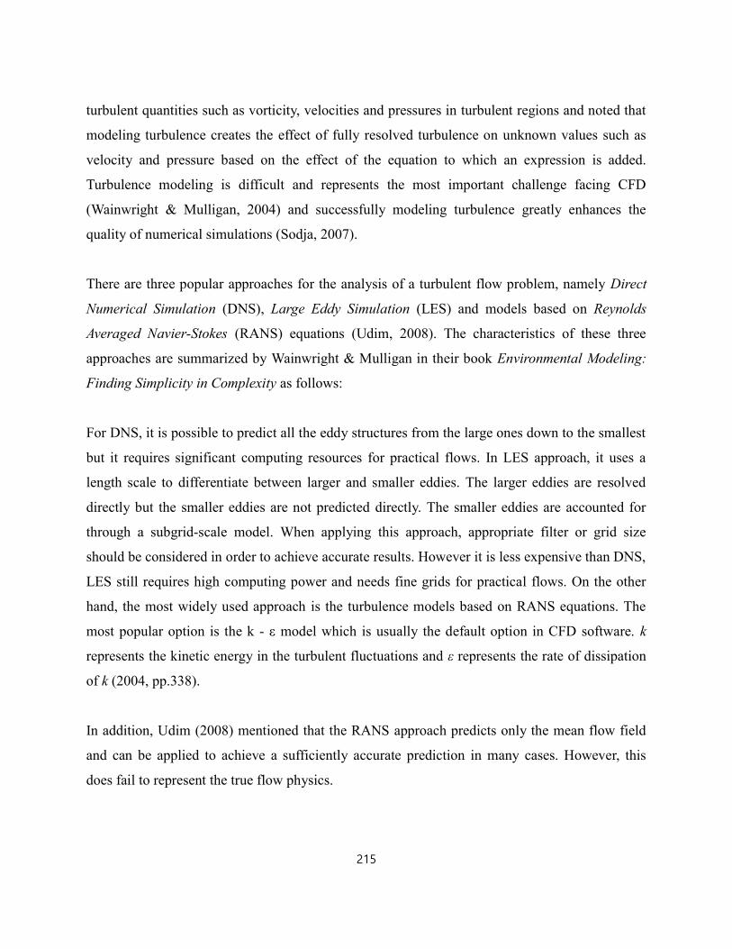
turbulent quantities such as vorticity, velocities and pressures in turbulent regions and noted that

modeling turbulence creates the effect of fully resolved turbulence on unknown values such as

velocity and pressure based on the effect of the equation to which an expression is added.

Turbulence modeling is difficult and represents the most important challenge facing CFD

(Wainwright & Mulligan, 2004) and successfully modeling turbulence greatly enhances the

quality of numerical simulations (Sodja, 2007).

There are three popular approaches for the analysis of a turbulent flow problem, namely Direct

Numerical Simulation (DNS), Large Eddy Simulation (LES) and models based on Reynolds

Averaged Navier-Stokes (RANS) equations (Udim, 2008). The characteristics of these three

approaches are summarized by Wainwright & Mulligan in their book Environmental Modeling:

Finding Simplicity in Complexity as follows:

For DNS, it is possible to predict all the eddy structures from the large ones down to the smallest

but it requires significant computing resources for practical flows. In LES approach, it uses a

length scale to differentiate between larger and smaller eddies. The larger eddies are resolved

directly but the smaller eddies are not predicted directly. The smaller eddies are accounted for

through a subgrid-scale model. When applying this approach, appropriate filter or grid size

should be considered in order to achieve accurate results. However it is less expensive than DNS,

LES still requires high computing power and needs fine grids for practical flows. On the other

hand, the most widely used approach is the turbulence models based on RANS equations. The

most popular option is the k - ε model which is usually the default option in CFD software. k

represents the kinetic energy in the turbulent fluctuations and ε represents the rate of dissipation

of k (2004, pp.338).

In addition, Udim (2008) mentioned that the RANS approach predicts only the mean flow field

and can be applied to achieve a sufficiently accurate prediction in many cases. However, this

does fail to represent the true flow physics.

In sum, although both the DNS and LES approaches provide better results, they require far

greater computer resources than turbulence models based on RANS methods. Furthermore, there

are a number of different versions of turbulence models based RANS methods now available

commercially (Udoewa & Kumar, 2012).

6. Solution algorithm

CFD simulations are constructed around numerical algorithms that can deal with fluid flow

problems. For example, consider the numerical algorithms used to resolve the coupling that

arises in the solution of Navier-Stokes equations between velocity, density and pressure

(Moukalled & Darwish, 2000). The SIMPLE (Semi-Implicit Method for Pressure Linked

Equations) type of algorithm is commonly used in CFD studies (Patankar & Spalding, 1972), but

over the years, a number of modified versions of the SIMPLE algorithm have been suggested

including the SIMPLER, SIMPLEC and PISO algorithms (Moukalled & Darwish, 2000).

Versteeg and Malalasekera (1995) compared those four algorithms in their book An Introduction

to Computational Fluid Dynamics: The Finite Volume Method. The SIMPLE algorithm was

originally proposed by Patankar and Spalding (1972) and is essentially a guess-and-correct

procedure for the calculation of pressure on a staggered grid arrangement. This method is

relatively straightforward and has been successfully used in numerous CFD procedures. The

SIMPLER (SIMPLE-Revised) algorithm is an improved version of the SIMPLE algorithm that

utilizes pressure corrections only to correct velocity fields. Consequently, this algorithm is very

effective in calculating the pressure field correctly and solving the momentum equations while at

the same time reducing the computing resources required. The book also introduces the

SIMPLEC and PISO algorithms. The SIMPLEC (SIMPLE-Consistent) algorithm follows the

same steps as the SIMPLE algorithm but defines the coefficients in the pressure-correlation

equation differently. The PISO algorithm, where the acronym PISO stands for Pressure Implicit

with Splitting of Operators, and implements a pressurevelocity calculation procedure for the

non-iterative computation of unsteady compressible flows. Versteeg and Malalasekera consider

that although the SIMPLEC and PISO algorithms have proved that they are as efficient as the

SIMPLER algorithm for certain types of flows, it is not clear whether they are better overall than

the SIMPLER algorithm.

7. Boundary conditions

After choosing a suitable mathematical model for the physical phenomenon, boundary conditions

must be chosen. For boundary-value problems, it is essential to assign values along the boundary

of the domain that will permit the problem to be solved throughout the entire 2D or 3D space.

There are two types of boundary conditions, namely Dirichlet and Neumann boundary conditions.

For a Dirichlet boundary condition, the fixed value of the unknown on the boundary is specified

for some flow problems; this is referred to as a direct boundary condition. In contrast, when the

value of a derivative of the unknown is specified, this is called a Neumann or natural boundary

condition. These boundaries are spatial boundaries (Udoewa & Kumar, 2012).

According to Wainwright & Mulligan (2004), it is common for the velocity to be fixed at an inlet

and outlet. For an inlet, turbulence quantities must be correctly specified and inlet profiles

consistent with the definition of roughness along the boundaries of the domain. For the outlet

condition, careful consideration must be given to the question of whether the outflow should

equal the inflow or whether the flow profile should be uniform along the stream direction in

order to avoid poor convergence or solutions that are not physically feasible.

8. Numerical parameters for controlling the calculation

Numerical parameters must be specified in order to control the calculation and reduce the

computational resources needed. These parameters include the relaxation factor, monitoring

residuals, different numerical schemes, the number of iterations for steady flow, number of time

steps for unsteady flow, and the choice between single and double precision.

Appendix C: Definitions of several CFD terms

CFD is a computer based mathematical modeling tool that is based upon the fundamental

governing equations of fluid dynamics. However, terms within CFD are often not obvious to

non-experts to that field (Souza, 2005). Thus, it is important to introduce and describe CFD

terms to them. While the most commonly used parameters of CFD will be introduced in this

chapter, several terms of CFD simulation will be introduced briefly in this section.

1. Aspect ratio

This is ratio of longest edge length to shortest edge length and it is a measure of quality for a

computational grid. In order to avoid convergence problems, the cell aspect ratios should be kept

as small as possible (Souza, 2005; STAR-CCM+ user guide 8.04).

2. Boundary conditions

The spatial or temporal specification of variable values or behavior to produce an unique solution

(Souza, 2005).

3. Convergence criteria

Through the iterations, the magnitude of the velocity divergence is reduced below some absolute

numerical value that tends to a single answer (Souza, 2005)

4. Divergence

The progression of a numerical scheme away from any single solution (Souza, 2005).

5. Grid / mesh

This is the outcome of discretizing the computational domain into a number of elements or cells

defining the discrete points at which the numerical solution is computed (Souza, 2005).

6. Grid density

This term means the number of cells in a given volume. A higher grid density should be applied

in regions of interest where the variables change rapidly so that their gradients can be computed

and represented accurately. In the case of lower grid density, it is generally used where the

solution is changing less in order to reduce the computational resources (Souza, 2005).

7. Invalid cell

When each cell interior face belongs to exactly two cells, this is considered as valid cell. If the

arrays storing the cell connectivity and vertices have entries that make reference to faces or

vertices that fall outside the expected range of values, invalid cells occur (STAR-CCM+ user

guide 8.04).

8. No-slip wall

This term means that the fluid velocity at the wall equals the wall velocity. The wall can rest or a

tangential wall velocity in the form of a velocity vector with respect to the laboratory coordinate

system can be specified (STAR-CCM+ user guide 8.04).

9. Schmidt number

A dimensionless number that is the ratio of kinematic viscosity to diffusivity (STAR-CCM+ user

guide 8.04).

10. Skewness

This term is an important measure of cell quality and it is designed to reflect whether the cells on

either side of a face are formed in such a way as to permit diffusion of quantities without these

quantities becoming unbounded (STAR-CCM+ user guide 8.04).

11. Slip wall

This term means that the fluid velocity at the wall is different with the wall velocity (STAR-

CCM+ user guide 8.04).

12. Structured grid

This grid forms a regular pattern. Its grid lines are continuous across the domain and are usually

aligned with the co-ordinate directions. For this grid, hexahedra in three dimensions or

quadrilaterals in two dimensions are included (Souza, 2005).

13. Unclosed cell

Generally a topologically closed volume cell consists of edges that are connected to exactly two

faces, and faces with normals pointing outwards. When a cell is missing a face, or the outward

normals are inconsistent, it is regarded as unclosed mesh (STAR-CCM+ user guide 8.04).

14. Unstructured grid

Unlike structured grid, this grid forms an irregular pattern. This grid allows highly complex

geometries to be modeled with relative ease compared to structured grids (Souza, 2005).

15. Wall functions

This function has been used to describe the effects of turbulent boundary layers in the region

adjacent to a wall, without resolving details of the near wall flow and eliminating the need for

high grid resolution in the viscous sub-layer (Souza, 2005).

Appendix D: The commercial CFD codes

Many commercial CFD codes such as STAR-CD and STAR CCM+ (CD-Adapco), FLUENT and

CFX (ANSYS, Inc.) or OpenFOAM have been used to simulate physical processes. These

commercial CFD packages include pre-processors to construct grids, and apply initial conditions,

processing algorithms that permit segregated or coupled, steady or unsteady state flows and a

variety of turbulence models, and post-processors that display results in a manner that enhance

interpretation. Among commercial codes, the characteristics of FLUENT and STAR-CCM+ have

been reviewed.

1. FLUENT

FLUENT is a most commonly used commercial CFD code. FLUENT solves the conservative

form of the Navier-Stokes equations using the finite volume method on an unstructured, non-

orthogonal, curvilinear coordinate grid system. Combinations of elements in a variety of shapes

are permitted, such as quadrilaterals and triangles for 2-D simulations and hexahedra, tetrahedra,

polyhedra, prisms and pyramids for 3-D simulations. Meshes can be created using mesh

generators (GAMBIT) or by several third-party CAD packages. FLUENT allows the following

file formats for importing are summarized in table 1 (ANSYS FLUENT, 12.0 User’s Guide).

Table 1 - File formats for importing into FLUENT (ANSYS FLUENT, 12.0 User’s Guide)

ABAQUS .inp, .fil, and .odb files

Mechanical APDL .inp, .cdb, .rst, .rmg, and .rfl files.

ANSYS CFX .def and .res files

CGNS files

EnSight files

ANSYS FIDAP Neutral files

GAMBIT files

HYPERMESH ASCII files.

NASTRAN Bulk Data files

PATRAN Neutral files.

PLOT3D mesh and result files.

Turbulent flow models including several popular k–epsilon and k–omega models, and the

Reynolds stress model (RSM) are available. Moreover, large eddy simulation (LES) and the

more economical detached eddy simulation (DES) turbulence models can be employed (ANSYS

FLUENT, 12.0 User’s Guide).

2. STAR-CCM+

STAR-CCM+ includes the general characteristics of FLUENT. In addition, STAR-CCM+ has a

single environment for whole CFD process such as solid modeling, mesh generation, post-

processing, etc. Moreover, STAR-CCM+ has a comprehensive suite of geometry creation and

preparation tools. For meshing, STAR-CCM+ employs the technology of hexahedral,

dodecahedral and arbitrary polyhedral cells and produces boundary trimmed meshes that

conform to geometry, as well as high quality prism layer meshes for accuracy. The following file

formats that can be imported into STAR-CCM+ are summarized in table 2 (STAR-CCM+ user

guide 8.04).

Table 2 - File formats for importing into STAR-CCM+ (STAR-CCM+ user guide 8.04)

Parasolid .x_t , .x_b

IGES .iges, .igs

STEP .stp, .step

Stereo lithography file .stl

PATRAN shells .pat

NASTRAN shells .nas

CATIA V4 .model, .exp, .session / CATIA V5 .catpart, .cadproduct

SolidWorks .sldprt, .sldasm

PRO/Engineer .prt, .asm

Autodesk Inventor .ipt, .iam

For turbulence models, various models that provide closure of the RANS equations, LES and

DES model are also available (STAR-CCM+ user guide 8.04).

3. The selection of CFD code

Reviewing manuals, similarities and differences between FLUENT and STAR-CCM+ in their

physics conditions such as turbulence types, grid discretization, and solving methods were

obtained. Although FLUENT is widely used and initially considered as a potential candidate for

this study, it has difficulties in creating models and meshes from other tools such as GAMBIT.

Moreover, the cost of its license ranges from $2,000 to $ 10,000 per year. In the case of STAR-

CCM+, it provides a single environment in which users can perform CAD creation to post-

processing and allows various types of file formats to be imported. In addition, free academic

license is provided. Thus, STAR-CCM+ was employed for this present study.