The analytical transfer functions ofwave-digital filters derived from

LC ladder prototypesE.C.Tan, Mem.I.E.E.E.

Indexing terms: Filters and filtering, Wave-digital filters

Abstract: Based on the wave-chain matrix technique, the paper presents some computationally efficient algo-rithms for obtaining the polynomial coefficients of the various analytical transfer functions of a class ofwave-digital filters derived from the resistance-terminated lossless LC ladder networks, given all the multipliercoefficients. It also describes the numerical methods for computing the multiplier coefficients from the com-ponent values of the associated reference filters. The applications of the algorithms in the studies of wave-digitalfilters are briefly discussed.

1 IntroductionWave-digital filters (WDFs) are a special class of recursivedigital filters obtained by employing known analoguedesigns and reinterpreting them in the digital domain by aseries of rather straightforward transformations [1, 2].They have been shown to exhibit the very promisingproperties of favourable coefficient sensitivity and lowroundoff noise. Numerical computations of WDF charac-teristics by means of wave-chain matrices are well known[3-5], but the employment of the same technique in deriv-ing the transfer function of a WDF in its analytical formfrom the given multiplier coefficients has remained unre-ported until recently [6], where it has been done for a classof WDFs derived from all-pole analogue filters. Thereasons are probably because (i) the multifeedback con-figuration of a WDF has, in general, a more complicated

practical realisation of WDFs, is the series and paralleladaptors with one matched port and the 2-port adaptors(Table 1). This class of elementary adaptors [12] will bechosen here for our purpose. Transfer functions of thelowpass (LP), highpass (HP), bandpass (BP) and the band-stop (BS) filters will be considered more or less individ-ually, the reason being that when the multiplier coefficientsare quantised, the familiar frequency transformations canno longer be accurately applied to the first-obtainedlowpass WDF transfer function as the nominal digitalcutoff frequency will be shifted. For the same reason, thebilinear transformation cannot be accurately applied to thes-domain transfer function to obtain the z-domain equiva-lent, unless the corresponding nonlinearity in the former isknown. The algorithms to be presented apply to any multi-plier coefficient, and will thus be more general and useful.

Table 1: Possible port-2 element for a 3-port adaptor

Port-2 element

Cmor L m

(Capacitor or inductor)

Series LC

Parallel LC

= ±z-1

(2,

Z"1 [2

(2c

ffm-1)z-1 +1

- 1 - ( 2 a m - 1 ) ]7 m - 1 ) z - 1 - 1

Explanation

inductor on dependentport, matched port asinput

same as above

structure and flow diagram than the corresponding con-ventional digital filter of the same order, since more arith-metic operations are involved, and (ii) the WDFrealisations are less modular than the conventional forms.Nevertheless, this paper will show that remarkably simplefactor-form numerator terms and efficient denominatorcoefficient algorithms of a wide range of WDF transferfunctions can be easily established by simple inductionsfrom a fairly general consideration of the wave-chainmatrix technique. (The algorithm presented in Reference 6represents only one of the few possible forms.)

In our discussions, the classical insertion loss analoguefilters on which the wave-digital equivalents are basedinclude the frequently encountered all-pole lowpass struc-ture and its frequency-transformed counterparts [7, 8](referred to as type-1 filters) and the elliptic prototypes[9]*. One choice of adaptors, which enables a convenient

* In the case of variable elliptic WDF realisations, the approximate componentvalues can be obtained by using a 2-dimensional cubic spline interpolation [10, 11].

Paper 2583G, received 15 December 1982

The author is with the Department of Electrical Engineering, University of Mel-bourne, Parkvillc, Victoria 3052, Australia

Notation

Some general notation= order of an analogue filter= order of the wave-digital equivalent

(= total number of unit delaysin a WDF)

n = section number of a filter= multiplier coefficient of parallel,

series and 2-port adaptor,respectively

= transfer function of an Nth orderWDF

= port resistances of adaptor and ofadaptor at port-2 respectively,i = port number (= 1, 2, 3)(see Figs. 3-7)

= corresponding port conductances= angular stopband edge frequency= angular cutoff frequency= normalisation frequency of elliptic

LP or HP filter

2.1nN

m = 1, 2,

HN(z) = Yn{z)lUJLz)

IEE PROCEEDINGS, Vol. 130, Pt. G, No. 5, OCTOBER 1983 185

co0 - = centre angular frequency of ellipticBP or BS filter (used fornormalisation in analogue case)

= selectivity factor= sampling period= normalised digital cutoff frequency= maximum allowable attenuation in

passband= minimum attainable attenuation in

stopband= bandwidth ratio for BP or BS filter

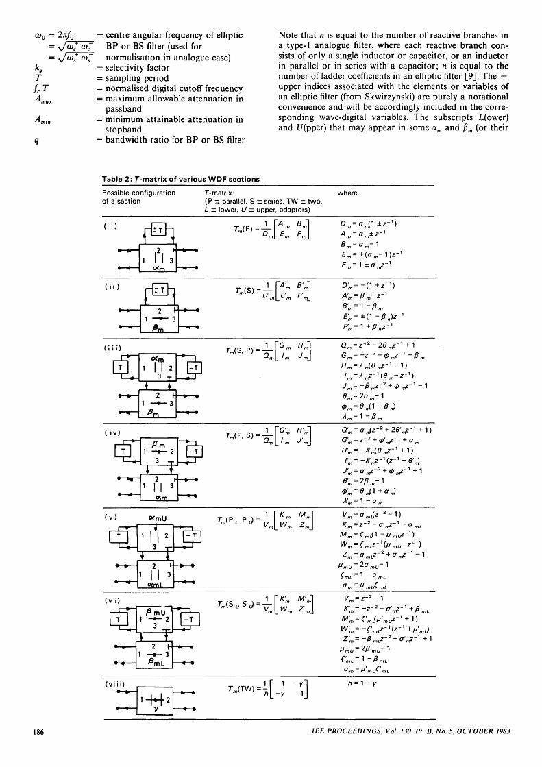
Note that n is equal to the number of reactive branches ina type-1 analogue filter, where each reactive branch con-sists of only a single inductor or capacitor, or an inductorin parallel or in series with a capacitor; n is equal to thenumber of ladder coefficients in an elliptic filter [9]. The ±upper indices associated with the elements or variables ofan elliptic filter (from Skwirzynski) are purely a notationalconvenience and will be accordingly included in the corre-sponding wave-digital variables. The subscripts L(ower)and t/(pper) that may appear in some am and /?m (or their

Table 2: 7-matrix of various WDF sections

Possible configurationof a section

7"-matrix:(P = parallel, S = series, TW = two,L = lower, U = upper, adaptors)

where

(I ) r-*

1

n

2 i ;

UP) — Am = a m±z-y

Bm=om-\Em= ±(am-1)z

( i i ) US)D'm\_E'

1 —*- 3

An

B'm='\ -

( i i i )

rr T l

fin

Qm = z - 2 - 2 0 / 7 / - 1 +1

Hm = .

9m = :

( i v )

3 - -

T (P ^\ =

J'm =

A' = 1 - a

Vm = amL{

/Wm = f m L ( 1 -

£. — O mlZ~

( v i )'mW U D J •/

l/'m = z " 2 - 1

/ C ' m = - z - 2 - (

M'm — £' mJjj' m\jZ~y + 1 )

W'm= - f 'm £z-1 (z- 1 +//'„Z ' m = ~P mL2

* tTIL *~ mL

(vii i)

1-r^-|-2y

= 1 r 1 -K-I

/iL-K 1J/? = 1 -

186 /££ PROCEEDINGS, Vol. 130, Pt. B, No. 5, OCTOBER 1983

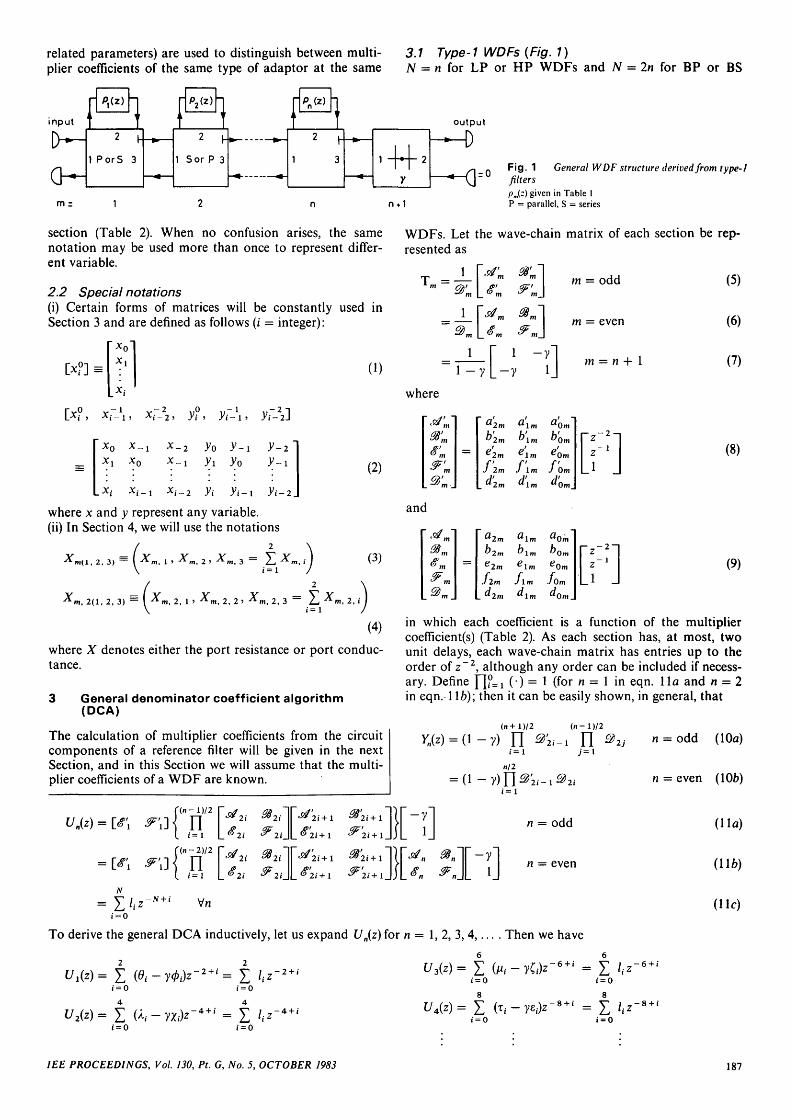
related parameters) are used to distinguish between multi- 3.1 Type-1 WDFs {Fig. 1)plier coefficients of the same type of adaptor at the same N = n for LP or HP WDFs and N — In for BP or BS

inputripi(z>h rip2(z)h

(H-1 PorS 3 1 Sor P 3

section (Table 2). When no confusion arises, the samenotation may be used more than once to represent differ-ent variable.

2.2 Special notations(i) Certain forms of matrices will be constantly used inSection 3 and are defined as follows (i = integer):

x 0

xx (1)

[x?, yf

x_

i - l A i -2 Ji }

where x and y represent any variable,(ii) In Section 4, we will use the notations

x Jx x x =Yw( 1, 2* 3) \ tn, 1 ' tn, 2 ' m, 3 / ^

yt_2

(2)

, 2(1, 2. 3) = , 2, 1 , 2, 2

i= 1

, 2, 3

(3)

m, 2 , i

where X denotes either the port resistance or port conduc-tance.

3 General denominator coefficient algorithm(DCA)

The calculation of multiplier coefficients from the circuitcomponents of a reference filter will be given in the nextSection, and in this Section we will assume that the multi-plier coefficients of a WDF are known.

N

i = 0Vn

Fig. 1 General WDF structure derived from type-1filterspm(:) given in Table 1P = parallel, S = series

WDFs. Let the wave-chain matrix of each section be rep-resented as

T = — = odd

m~ e v e n

m = n + 1

(5)

(7)

where

0m

b'2m b\m b'Ome2m elm e0mf f f

J 2m J l m J 0m

- l (8)

and

2m

2m 0m

J2m Jim JO" l m " 0 m .

(9)

in which each coefficient is a function of the multipliercoefficient(s) (Table 2). As each section has, at most, twounit delays, each wave-chain matrix has entries up to theorder of z~2, although any order can be included if necess-ary. Define Y\?=i (") = 1 (f°r « = 1 in eqn. l l a and n = 2in eqn. 116); then it can be easily shown, in general, that

(n-D/2

n ^2i-i n •; = i j=\

nil

n = odd

= even

n = even (106)

(Ha)

(116)

(He)

To derive the general DCA inductively, let us expand Un(z) for n = 1, 2, 3, 4 , . . . . Then we have

i = 0

i = 0

t= Z lii = 0

ti = 0 i = 0

i = 0

8

i = 0 i = 0

- 6 + i

/ £ £ PROCEEDINGS, Vol. 130, Pt. G, No. 5, OCTOBER 1983 187

where

n= 1

r>oi ro o o o i o on(/>! = 0 0 0 0 0 1 0 [0 0 0 e'21 e\

Ltf>2J Lo o o o o o I Jf0o i ro o o o i o on\ e, = o o o o o I o [o o o /'-L02J Lo o o o o o iJ

21 J 11 J OlJ

n = 2

n = 3

/ 22

fl'13 a'O3 e'22

ft'13 b'O3 / ' „

/2

e'02Y

_ 2 = O , 6»_2 = 0_ 1 = O , 0 _ 1 = O03 = 0, 6>3 = 004 = 0, 04 = 0

Z - i = O , A _ 1 = 0Xs = 0, A5 = 0X6 = 0, X6 = 0

C - i = O , /*_! = 0C7 = 0, nn = 0C8 = 0, A*8 = 0

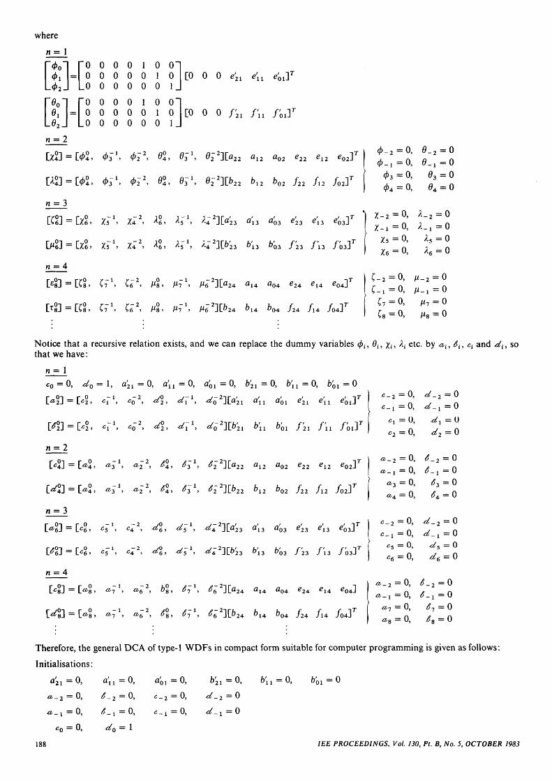
Notice that a recursive relation exists, and we can replace the dummy variables </>,-, 0,,that we have:

n = 1

etc. by <»,-, ^,, c; and ^,-, so

« ^

'21 / ll l

02

/ 22

b'O3 f23 f\3 fQ3y

/04]

0, d^ = u0, ^ 2 = 0

^3=0, ^3=0

^ 4 = 0, 6A = 0

= 0, ^5=0

= 0, d6 = 0

_j = 0 , ^_i = 0

^7 = 0, ^7 = 0

^ 8 = 0» ^8 = 0

Therefore, the general DCA of type-1 WDFs in compact form suitable for computer programming is given as follows:

Initialisations:

a'2l = 0, a'iy = 0, a'0l = 0, b'21 = 0, b'lt = 0, b'ol = 0r\ /> rv (\ / f\

• O _ 2= = U , O _ 2 — " , C _ 2 — U, •Co —2 — \j

a.1=0, ^ _ 1 = 0 , c _ 1 = 0 , ^ _ ! = 0

c0 — 0, ^ 0 = 1

188 1EE PROCEEDINGS, Vol. 130, Pt. B, No. 5, OCTOBER 1983

For m = odd,

- l = 0 > C2m =

c2m-\->

'c2m-2>

If m = n, go to (\

For m = even,

- r^o'2m-

- 1 - 2

L- If m = n, go to (2)

: C'SJ = CflJ " yC«SJ end;

fl0m C2m e'l

Om /'2m / ' l

lm aOm e2m film

'lm &Om flm / l m

end.

Obviously, other forms of DCA can be easily obtained by combining terms in [ •• ] T with the same z1 (i = 0, — 1, —2) andthus the numbers of columns in the middle matrix can be accordingly reduced.

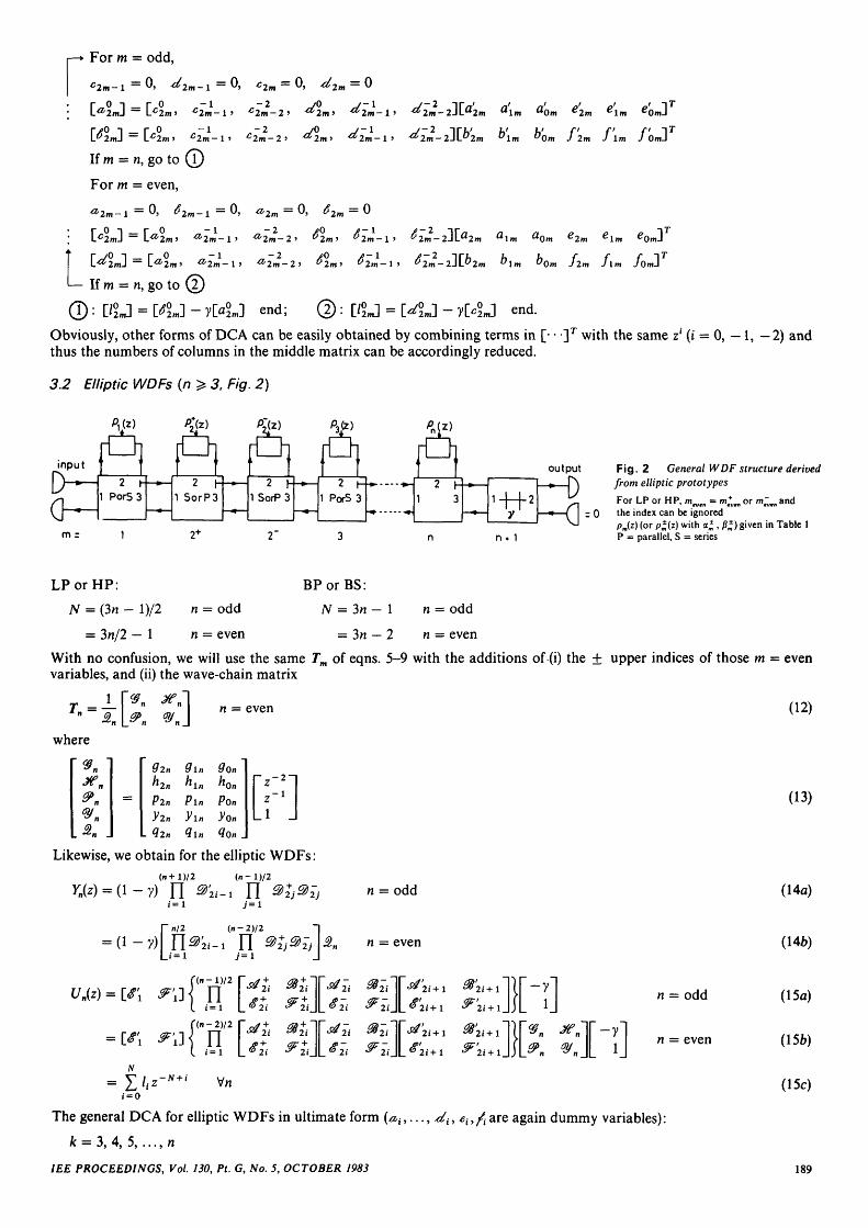
3.2 Elliptic WDFs (n 3, Fig. 2)

rfiiinput t t t t> — , I I I I

DG

2 h1 PorS3

—»— 2 h1 SorP3

h rl)

"I• I f f

2 h1 SorP3

2 (-

1 PorS 3

•s?a2 h

1 3 ++••

output

n* 1

Fig. 2 General WDF structure derivedfrom elliptic prototypes

For LP or HP, mnm = m^,,,n or m~vtlt andz 0 the index can be ignored

pm(z) (or p*(z) with a^ , /?*) given in Table 1P = parallel, S = series

LPorHP: BPorBS:

N = (3n - l)/2 n = odd N = 3n - 1 n = odd

= 3n/2 — 1 n = even = 3n — 2 n = even

With no confusion, we will use the same Tm of eqns. 5-9 with the additions of (i) the ± upper indices of those m = evenvariables, and (ii) the wave-chain matrix

J f

where•] -

9ln 90n

Kn KnPin Ponym yon9ln <lOn

even

[r]Likewise, we obtain for the elliptic WDFs:

(n-D/2

[ nil (n-2)/2

n^2I-i n i

n = odd

n = even

M, - N + i2

i = 0

n = odd

n = even

The general DCA for elliptic WDFs in ultimate form (<*,,

k = 3, 4, 5, . . . , n

IEE PROCEEDINGS, Vol. 130, Pt. G, No. 5, OCTOBER 1983

di, «,,/, are again dummy variables):

(12)

(13)

(14a)

(15a)

(156)

(15c)

189

Initialisations:

1—•

\

/o — J2\i A~fll> /2—JOI

_2=0, ^-2=0, «-2=0,

-1=0, ^ - !=0 , «-!=(>,

For k = odd,

N = 3k - 1

^ - 5 = 0 , 4N-4. = 0, / N _ 5 =0, /;v_4 = 0

^ _ 2 = 0 ,

_ r O - 1 - 2 / - 2 -|r\~ +iV-6JLa2(k-2(k

+

aO(k-l) e2(fc-

°O(k-l) J 2 ( l -

eO(k-l)J

7 l(k-l(k-l)

- 3 'iV-4

- 1 = 0, «N = 0, ^ N _ x = 0,

] = [* fi ^ ^

= 0

L

If k = n, go to (3)

For fc = even,

N = 3/c - 2

-eN_1=0, ^N = 0,

[4 %% - 2

If fc = n, go to

end ©: [/J] =J] = end

e2(fc-l) e l (k- l ) eO(k-l)J-._ . _ . _ - . r

;2(k- l ) 7 l (k - l ) 7O(k-l)J

f 2k f Ik

Plk

For elliptic LP or HP WDFs, only one ofwhose analytical transfer functions can be easily derivedfrom the presented DCAs and eqns. 5-15, by suitable sub-stitutions of the wave-chain matrices in Table 2, accordingto the adaptor combinations in Table 3. Yn(z) of those

is used. Suppose the first one is chosen, then the other WDFs are listed in Table 4.should be set equal to the identity matrix as

4 Computations of multiplier coefficients

Rt x (= Rs) and R, are given. For LP WDFs, Y = C andand the corresponding entries are to be substituted in the X = L; for HP WDFs, Y = 1/L and X = 1/C. Let A =appropriate places of the DC A. ^ 3 1 Rl)/(Rn 3 + Rt) and define the notation

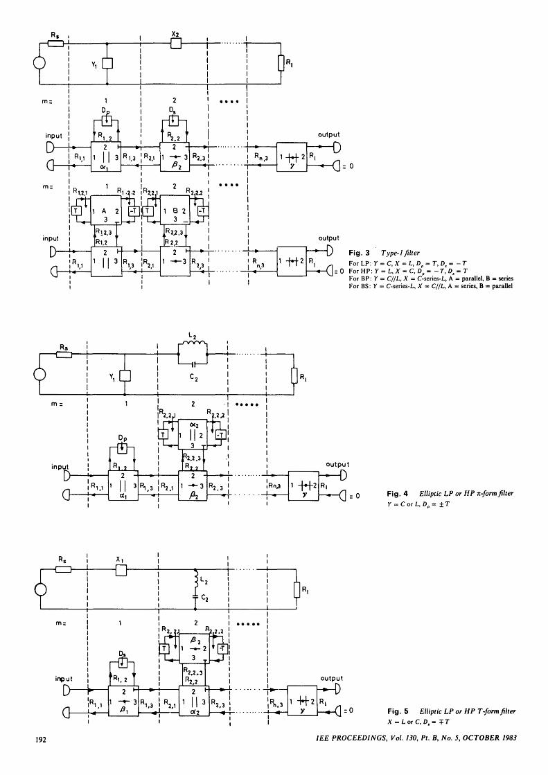
3.3 Some common filter circuitsFigs. 3-7 show some of the most commonly used analoguetype-1 and elliptic filters and their wave-digital equivalents

If m = n (n = odd), go to (n^If m = n — 1 (n = even), go to (n

= branch (if nodd—» (f\1) 5 "even'

Table 3:Section

Combinations of sections for the WDFsType-1 WDF

LPor HP BP BS LPor HP-;: BP-7t

Elliptic WDF

BS-TI LP or HP-T BP-T BS-T

m - 1 . 3 . 5 n;(n = odd) TJP)*= 1, 3, 5 n - 1 ; (n = even)

m-2. 4, 6 n - 1; (n - odd) TJS)*

= 2. 4, 6 n - 2 ; (n = even)

TJS)* T JS L, S J 7JS, P) 7"J[S)*

rm(TW)

L. P J T J[P. S) 7 J P ) * T J^P L, P ,) 7"j(P, S) T J S ) *

L. S J T JS , P) T j(S, P) T*J[S. P) T*J[S. P) T JP, S)

t. S J T JS , P) T J P ) *

L, S J TJS.P)

%P, S) r*j[P. S)

L, PJ T JP . S)

Corresponding to the appropriate unit delay

190 IEE PROCEEDINGS, Vol. 130, Pt. B, No. 5, OCTOBER 1983

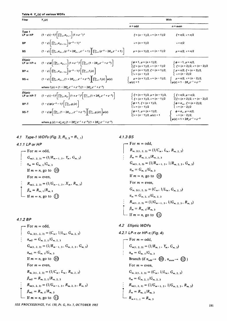
Table 4: YJz) of various WDFs

Filter Yn(z)

n = odd

With

n = even

TypeiLP or HP

BP

BS

(1 -K)(-1)c[n;-i«'a/-i](1 i*-1)" f = ( n - 1 ) / 2 , v = ( n + 1)/2

v = (n + 1 )/2

A/ = (n + 1 )/2, v = (n - 1 )/2

(=n/2,v = n/2

v = n/2

y, = n/2, v = n/2

EllipticLPorHP-n ( 1 -

BP-7T (1 -

BS~7t ( I ~

where f,

: . i <»2/-iJi(1 " ^ [ f l L i 0 " Zfl,,*"1

1)/2.v=(n-1)/21 )/2.f// = (n + 1 )/2, f = (n +

llv = (n-1) /2^ = (n + 1 )/2, v = (n - 1 )/2,

(=(n + 2)/2, v=(n-2)/2/y = n/2, f=(n + 2)/2,v=(n-2)/2

// = n/2, v = (n - 2)/2,?) = 1 -2«nz- '+z-2

= (1 -20+,z-1 + z-2)(1 - 2 0 ^ - ' + z"2)

Elliptictlliptic r -i r -iLP or HP-T d -K)(-D{| nJ-iflUO ±«-1)«l fl ' i-id +2»'2,z-1 +z-2)J

BP-T

BS-T d -

where g((z) = oj,a2,(

f = ( n + 1)/2, v = ( n - 1 ) / 2

v = (n - 1 )/2

+ 20'2-z-' +z"2)

I (=n/2,v = n/2,[|f=(n + 2)/2, v=(n-2)/2

v=(n-2)/2p = an,fj = n/2.v = (n - 2)/2,r)=1 +2d'z"'+z-2

4.7 T/pe- 7 H/DFs (F/gr. 3, /?0 3 =

4.7.7 LPorHP

For m = odd,r 1 , 2 , 3) •

fn fn, 1/ m, o

If m = n, go to

For m = even,

, 3)

- i , 3 ,

Pm = -^m, l /^m, 31 If m = n, gO tO (fl)

, 3)

4.1.2 BP

r For m = odd,

Gm, 2(1, 2, 3) = (Cm » V^m , ^ m > 2, 3)

I amC/ = Gm, 2, l /GM i 2, 3

G m ( i , 2, 3) = ( V K m - 1, 3 » Gm, 2, 3 » Gm, 3)

amL = Gm, l/Gm, 3

If m = n, go to @)

For m = even,

^ m 2 , 3)

2) 3) = ( l / G m - 1, 3 > Km 2, 3 > Km 3)

= Km, JRm< 3

If W = n, gO tO (lj)

IEE PROCEEDINGS, Vol. 130, Pt. G, No. 5, OCTOBER 1983

Km, 2(1, 2, 3)

PmU = Km, 2, l/Km_ 2, 3

4.1.3 BS

r For m = odd,

, 2(1, 2, 3)

= ^m, 2, , 2, 3

> 3

If m = n, go to

For m = even,

,, 2, 3

, 2(1. 2, 3)

— If m = n, go to (fl)

4.2 £///pf/c H/DFs

4.2.7 LP-norHP-n(Fig.4)

I—> For m = odd,

2 3)

2, 3» Gm, 3)

, 3)

Gm(l, 2. 3) = (VK m , x , Ym, Gm 3)

am = Gm, X/Gm> 3

Branch (if nodd^ © , nevm^> @ )

For m = even,

Gm, 2(1, 2, 3) = (Cm > V^m > ^ m 2 3)

am = Gm, 2, l/Gm, 2> 3

^ ( l , 2 , 3 ) = ( l / G m - i , 3 . VGm,2,3> Rm, 3)

^m = Km > 1 / / ? m § 3

^ m + 1 , 1 = Km 3

191

output

—•"—D Fig. 3 Type-1 filterR. ForLP: Y = C, X , Ds= -T

«—Q = 0 For HP: Y = L, X = C, Dp = -T, Ds = TFor BP: y = C//L, X = C-series-L, A = parallel, B = seriesFor BS: Y = C-series-L, X = C//L, A = series, B = parallel

0 F i g . 4 Elliptic LP or HP n-form filter

Y = C or L,D= ±T

a Fig. 5 Elliptic LP or HP T-form filterX = L or C, Ds = T 7

192 IEE PROCEEDINGS, Vol. 130, Pt. B, No. 5, OCTOBER 1983

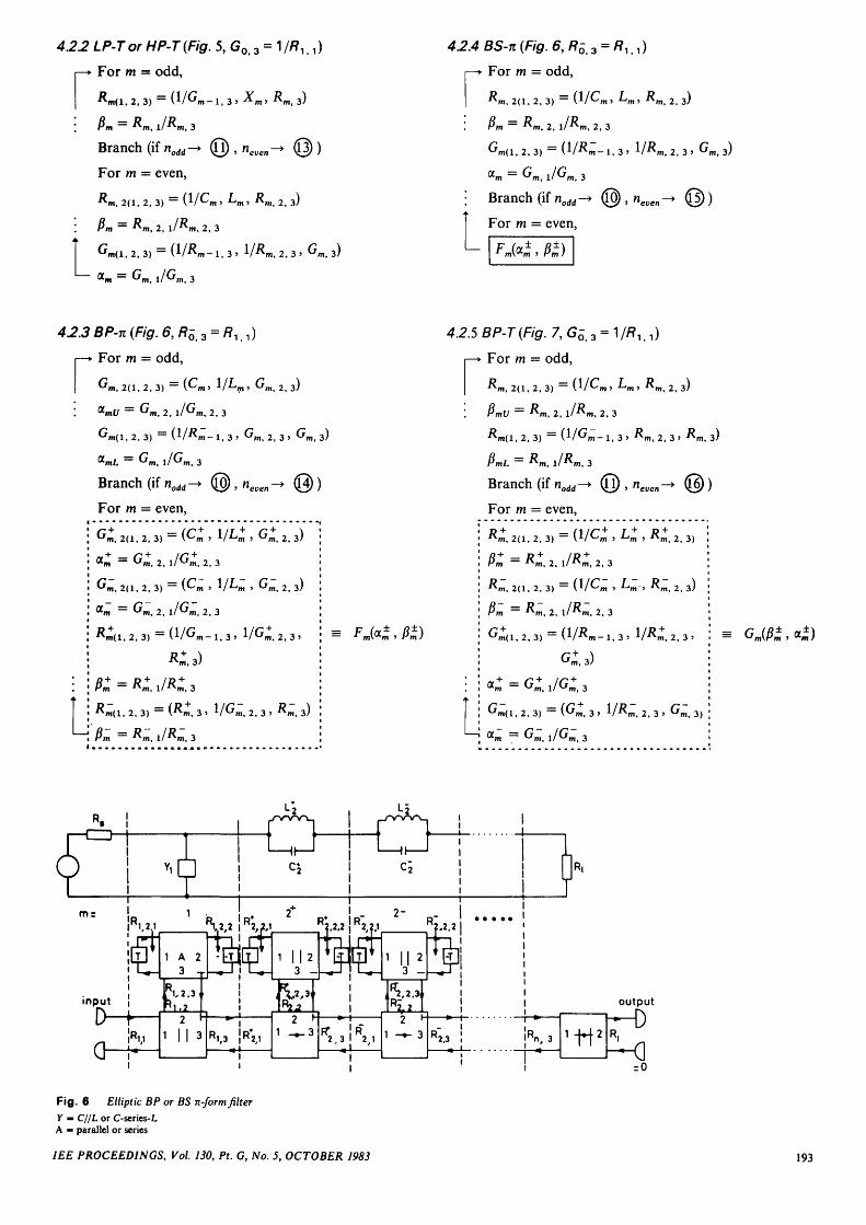
422 LP-T or HP-T {Fig. 5, Go, 3 = 1 //?, t ,

r For m = odd,

^ m ( l . 2, 3) = ( V ^ m - 1, 3 » ^m > -^m, 3)

I ftn = ^m, l/^m, 3

Branch (if nodd-> ( 0 ) , nmm-+ @ )

For m = even,

•^m. 2(1. 2, 3) = ( V O n > ^m > ^m, 2, 3)

i 0m = ^m, 2, l / ^ m , 2, 3

m ( l , 2 , 3 ) . 2 , 3 > ^ m . 3)

For m = odd,

Km, 2(1, 2, 3) = ( V ^ m , Lm , Rm 2 3)

0m = Km> 2, JR-m, 2, 3

, 3

Branch (if nodd-> © , ncuen

For m = even,

, 3

For m = odd,

Gm. 2(1. 2. 3) = (Cm » V-^m » G m , 2. 3)

am(/ = ^m, 2. l / ^ m . 2. 3

L, 2, 3) ~ W J v m - 1, 3 » Gm, 2, 3 > G m 3/

amL ~ u m , l / u m , 3

Branch (if nodd-> © , neven-+ @)

For m = even,

G m .

<

Gm,

« m

0m+

K (

0m

2(1

= (

2(1

2 ,

' « .

2 ,

= Gm,

1. 2,

= /

c,3)

lm.

3)

2 ,

3)

2 ,

=

= (Cm>l/Gm 2

= (C~,

\/Gm o

K*)< 3

\ m 3 »

K"3

3

3

1/G

-m . Gm, 2.

m, 2, 3 ' ^ r

3 )

3)

n, 3) :

4.2.5 BP-T(Fig. 7,Go,3

r For m = odd,

K m , 2(1, 2, 3) = ( V ^ m > - m > ^m, 2, 3)

0mU = K m , 2 , l / ^ m > 2, 3

^ m ( l , 2 , 3 ) = ( V G m _ i i 3 , ^ m , 2,3> -^m, 3)

PmL = Km, i / /? m , 3

Branch (if nodd-> @ , neven-^ © )

For m = even,

, 2(1, 2, 3) = (V^m > Lm , Rm 2 , 3)

0m = Rm, 2, l/Km, 2, 3

°m, 2(1, 2. 3) = ( V C m , Lm-, Rm 2, 3)

0m = # " , 2. l /^ m , 2. 3

2, 3) = (Gm, 3 > , 2 , 3 > ^m, 3)

, 3

Fig. 6 Elliptic BP or BS n-form filterY - C//L or C-serics-LA - parallel or series

IEE PROCEEDINGS, Vol. 130, Pt. G, No. 5, OCTOBER 1983 193

output

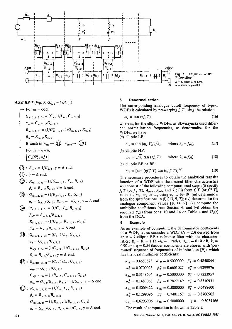
Fig. 7 Elliptic BP or BS1 n T-formfilter

*\\ X = C-series-L or C//LrO A = series or parallel

4.2.6

r For m = odd,

Gm, 2(1, 2, 3) — (^m >

! <*m = Gm. 2, l/Gm, 2, 3

^m(l , 2, 3) = ( V ^ m - 1, 3

/?m = -^m, l /^m, 3

: Branch (if nodd-> @

For m = even,

2, 3)

m> 2 , 3 > # m , 3)

, «*)

© : JRn,3 = l /G n , 3 , y =

(0) : y = A end.

QJ' • ^ B ( 1 . 2, 3) = ( V ^ n - 1 . 3 > -^n > * V 3)

«„ = Gn, JGHt 3, /?„, 3 = VGn, 3, y = A end.

© : ^n.2(i,2.3) = (l /Cn,Ln, JRn,2 ,3)

PnU = ^n . 2, l /^n , 2, 3

^n( l , 2. 3) = (V^m, 3 > ^n , 2, 3 > ^ B , 3)

PnL = ^n . l / ^n . 3 » V = A e n d .

QJ) : ^n, 2(1, 2, 3) = (^n > V-^B > ^ B , 2, 3)

«n = Gn, 2 , l /Gn , 2, 3

# B ( 1 , 2. 3) = U/G M f 3 » 1/^n. 2, 3 . ^n , 3)

: Gn. 2(1,2,3) = (Cn» V^n» G B , 2. 3)

aBl/ = GBf 2, l/Gflt 2, 3

^fl(l. 2, 3) = (V^m, 3 > Gn, 2 , 3 > ^ B , 3)

ani = Gn, i/G^ 3 , KB. 3 = 1/Gn, 3 , y = A end.

Pn = ^ B , 2, B. 2 , 3

, 3 > V ^ B , 2, 3 > Gn> 3)G n ( l , 2, 3)

«„ = Gn. i/G.. 3, K, 3 = VGn> 3 , y = A end.

(17)

(18)

(19)

5 DenormalisationThe corresponding analogue cutoff frequency of type-1WDFs is calculated by prewarping/c T using the relation

coc = tan (nfc T) (16)

whereas, for the elliptic WDFs, as Skwirzynski used differ-ent normalisation frequencies, to denormalise for theWDFs, we have:(a) elliptic LP:

coB = tan (nfc T)/y/ka where k, =fc/fs

(b) elliptic HP:

C*>B = yfis tan (nfe T) where ks =fjfc

(c) elliptic BP or BS:

(D0 = [tan (nf? T) tan (*/" T)]1 / 2

The necessary procedures to obtain the analytical transferfunction of a WDF with the desired filter characteristicswill consist of the following computational steps: (i) specifyfc T ( o r / ± T), Amax, Amin and ks; (ii) from/f T ( o r / * T),calculate coc, coB or co0 using eqns. 16-19; (iii) determine nfrom the specifications in (i) [13, 9, 7]; (iv) denormalise theanalogue component values [8, 14, 9]; (v) compute themultiplier coefficients from Section 4; and (vi) obtain therequired Yn(z) from eqns. 10 and 14 or Table 4 and Un(z)from the DCA.

6 Example

As an example of computing the denominator coefficientsof a WDF, let us consider a WDF (AT = 20) derived froman n = 1 elliptic BP-TT reference filter with the character-istics: Rs = Rt = 1 Q, (o0 = 1 rad/s, Amax = 0.10 dB, k3 =0.90 and q = 0.54 (ladder coefficients are chosen with 'per-muted' sequence of frequencies of infinite loss [9]), whichhas the ideal multiplier coefficients:

alL = 0.4680823 aw = 0.5000000

a2+ = 0.0700023 j?2~ = 0.6601027

a3L = 0.3148604 a3l/ = 0.5000000

fa = 0.7827149

a5U = 0.5000000

fc = 0.7401157

a+ = 0.1489068

a5L = 0.5009422

a " = 0.1299096

a7L = 0.6293906

^ = 0.4850844

a j = 0.9299976

jS^ = 0.7223957

a^ = 0.8510931

fc = 0.6488600

a6" = 0.8700902

y = -0.3034166

194

alv = 0.5000000

The result of computation is shown in Table 5.

IEE PROCEEDINGS, Vol. 130, Pt. B, No. 5, OCTOBER 1983

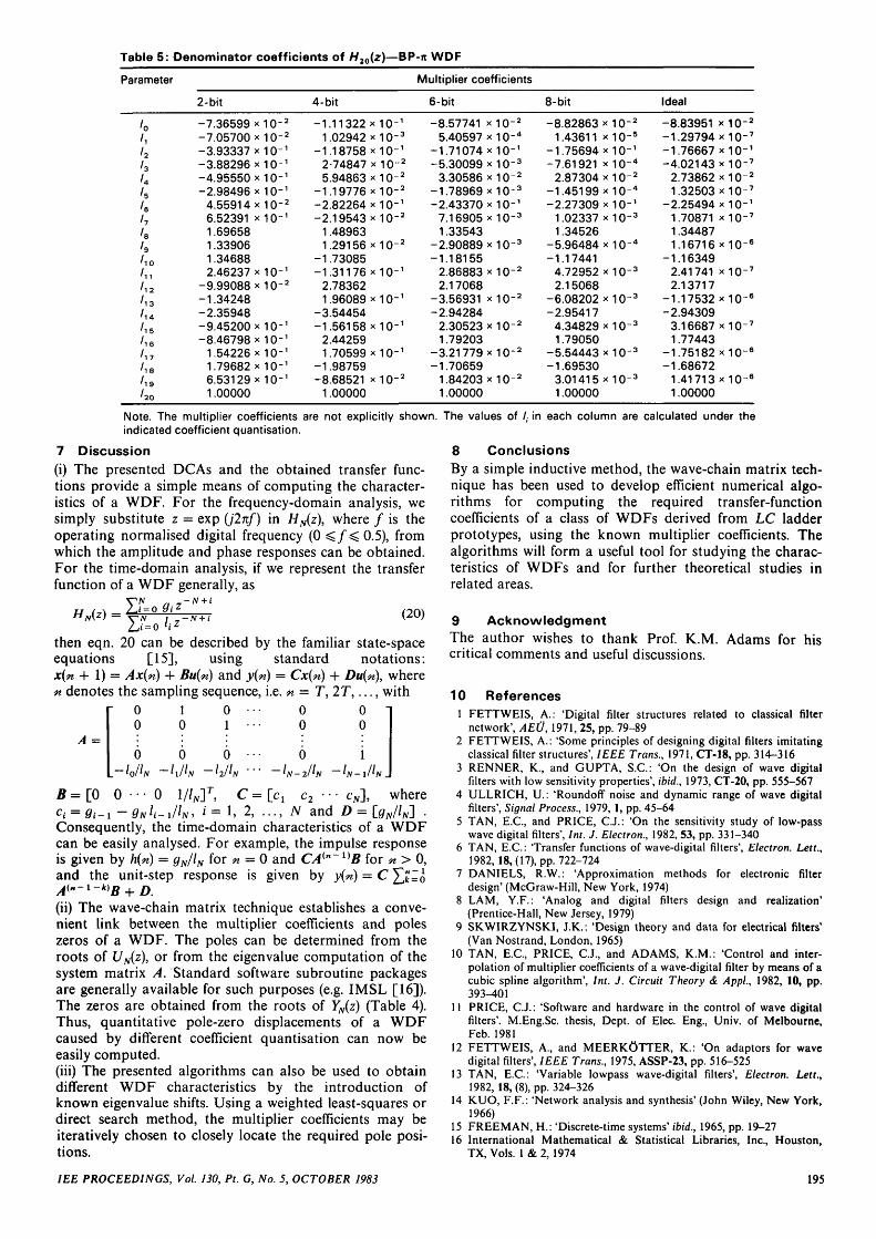
Table 5: Denominator coefficients of H20(z)—BP-rr WDF

Parameter

'o/,l2l3UuUI-,UIt

/ 1 0

/11

/ 1 2

' 1 5

' i e

/ w

' i s

' i 9

/ 2 0

2-bit

-7.36599 x 10"'-7 .05700x10"-3.93337x10--3.88296x10--4.95550x10"-2.98496x10-

4.55914 x 10-6.52391 x i o -1.696581.339061.346882.46237 x i o -

-9.99088x10--1.34248-2.35948-9.45200x10"-8.46798 x 10"

1.54226 x 10"1.79682 x 10"6.53129x10"1.00000

4-bit2 - 1 .11322x io - 1

2 1.02942 x i o - 3

-1.18758 x 10-1

2-74847 x 10-2

5.94863 x 1 0 - 2

-1.19776 x 10-2

2 -2.82264 X 1 0 - 1

-2.19543 x 10-2

1.489631.29156 x i o - 2

-1.73085-1.31176 x i o - 1

2 2.783621.96089 x i o - 1

-3.54454-1.56158 x i o - 1

2.442591.70599 x i o - 1

-1.98759-8.68521 x i o - 2

1.00000

Multiplier coefficients

6-bit

-8.57741 x i o - 2

5.40597 x i o - 4

-1.71074 x i o - 1

-5.30099 x i o - 3

3.30586 x i o - 2

-1.78969x10-3-2.43370 x i o - 1

7.16905X10-3

1.33543-2.90889 x lO- 3

-1.181552.86883 x 10-2

2.17068-3.56931 x i o - 2

-2.942842.30523 X 1 0 - 2

1.79203-3.21779 x i o - 2

-1.706591.84203 X 1 0 - 2

1.00000

8-bit

-8.82863 x 10-2

1.43611 x 10-5

-1.75694 x i o - 1

-7.61921 x i o - 4

2.87304 x i o - 2

-1.45199 x 10-4

-2.27309 x 10-1

1.02337x10-31.34526

-5.96484 x 10-4

-1.174414.72952 x 10-3

2.15068-6.08202x10-3-2.95417

4.34829 x lO- 3

1.79050-5.54443 x 10-3

-1.695303.01415 x 10-3

1.00000

Ideal

-8.83951 x i o - 2

-1.29794 x i o - 7

-1.76667 x i o - 1

-4.02143 x 10-7

2.73862 x i o - 2

1.32503 x i o - 7

-2 .25494x10- '1.70871 x i o - 7

1.344871 . 1 6 7 1 6 X 1 0 - 6

-1.163492.41741 x 10-7

2.13717-1.17532 X 1 0 - 6

-2.943093.16687 x i o - 7

1.77443-1.75182 x i o - 6

-1.686721.41713 x 10-6

1.00000

Note. The multiplier coefficients are not explicitly shown. The values of /, in each column are calculated under theindicated coefficient quantisation.

7 Discussion(i) The presented DCAs and the obtained transfer func-tions provide a simple means of computing the character-istics of a WDF. For the frequency-domain analysis, wesimply substitute z = exp (J2nf) in HN(z), where / is theoperating normalised digital frequency (0 J ^ / ^ 0 . 5 ) , fromwhich the amplitude and phase responses can be obtained.For the time-domain analysis, if we represent the transferfunction of a WDF generally, as

nN\z) — (20)

then eqn. 20 can be described by the familiar state-spaceequations [15], using standard notations:x(n + 1) = Ax{n) + Bu{n) and y(n) = Cx(n) + Du{?i), wheren denotes the sampling sequence, i.e. n = T,2T,..., with

A =

00

6•loll.

whereB=[0 0 ••• 0 1//N]T, C=[c1 c2 ••• CJVCi = 0 i - i - ONII-I/IN, * = !> 2> •••> N and D = [#„//„] .

Consequently, the time-domain characteristics of a W D Fcan be easily analysed. For example, the impulse responseis given by h{n) = gN/lN for n = 0 and CA{n~l)B for n > 0,and the unit-step response is given by y(n) = C Yj< = oA(nlk)B+ D.(ii) The wave-chain matrix technique establishes a conve-nient link between the multiplier coefficients and poleszeros of a WDF. The poles can be determined from theroots of UN(z), or from the eigenvalue computation of thesystem matrix A. Standard software subroutine packagesare generally available for such purposes (e.g. IMSL [16]).The zeros are obtained from the roots of YN(z) (Table 4).Thus, quantitative pole-zero displacements of a WDFcaused by different coefficient quantisation can now beeasily computed.(iii) The presented algorithms can also be used to obtaindifferent WDF characteristics by the introduction ofknown eigenvalue shifts. Using a weighted least-squares ordirect search method, the multiplier coefficients may beiteratively chosen to closely locate the required pole posi-tions.

8 ConclusionsBy a simple inductive method, the wave-chain matrix tech-nique has been used to develop efficient numerical algo-rithms for computing the required transfer-functioncoefficients of a class of WDFs derived from LC ladderprototypes, using the known multiplier coefficients. Thealgorithms will form a useful tool for studying the charac-teristics of WDFs and for further theoretical studies inrelated areas.

9 AcknowledgmentThe author wishes to thank Prof. K.M. Adams for hiscritical comments and useful discussions.

10 References1 FETTWEIS, A.: 'Digital filter structures related to classical filter

network', AEU, 1971, 25, pp. 79-892 FETTWEIS, A.: 'Some principles of designing digital filters imitating

classical filter structures', IEEE Trans., 1971, CT-18, pp. 314-3163 RENNER, K., and GUPTA, S.C.: 'On the design of wave digital

filters with low sensitivity properties', ibid., 1973, CT-20, pp. 555-5674 ULLRICH, U.: 'Roundoff noise and dynamic range of wave digital

filters', Signal Process., 1979, 1, pp. 45-645 TAN, E.C., and PRICE, C.J.: 'On the sensitivity study of low-pass

wave digital filters', Int. J. Electron., 1982, 53, pp. 331-3406 TAN, E.C.: 'Transfer functions of wave-digital filters', Electron. Lett.,

1982, 18,(17), pp. 722-7247 DANIELS, R.W.: 'Approximation methods for electronic filter

design' (McGraw-Hill, New York, 1974)8 LAM, Y.F.: 'Analog and digital filters design and realization'

(Prentice-Hall, New Jersey, 1979)9 SKWIRZYNSKI, J.K.: 'Design theory and data for electrical filters'

(Van Nostrand, London, 1965)10 TAN, E.C, PRICE, C.J., and ADAMS, K.M.: 'Control and inter-

polation of multiplier coefficients of a wave-digital filter by means of acubic spline algorithm', Int. J. Circuit Theory & Appi, 1982, 10, pp.393-401

11 PRICE, C.J.: 'Software and hardware in the control of wave digitalfilters'. M.Eng.Sc. thesis, Dept. of Elec. Eng., Univ. of Melbourne,Feb.1981

12 FETTWEIS, A., and MEERKOTTER, K.: 'On adaptors for wavedigital filters', IEEE Trans., 1975, ASSP-23, pp. 516-525

13 TAN, E.C: 'Variable lowpass wave-digital filters', Electron. Lett.,1982, 18, (8), pp. 324-326

14 KUO, F.F.: 'Network analysis and synthesis' (John Wiley, New York,1966)

15 FREEMAN, H.: 'Discrete-time systems' ibid., 1965, pp. 19-2716 International Mathematical & Statistical Libraries, Inc., Houston,

TX, Vols. 1 & 2, 1974

IEE PROCEEDINGS, Vol. 130, Pt. G, No. 5, OCTOBER 1983 195