The Agency Model and MFN Clauses

JUSTIN P. JOHNSON†

January 25, 2017

Abstract. I provide an analysis of vertical relations in markets with imperfect

competition at both layers of the supply chain and where exchange is intermediated

either with wholesale prices or revenue-sharing contracts. Revenue-sharing is ex-

tremely attractive to firms that are able to set the revenue shares but often makes

the firms that set retail prices worse off. This is so whether revenue-sharing low-

ers or raises industry profits. These results are strengthened when a market moves

from “the wholesale model” of sales to “the agency model” of sales, which results

in retailers setting revenue shares and suppliers setting retail prices. I also show

that retail price-parity restrictions raise industry prices. These results provide a

potential explanation for why many online retailers have adopted the agency model

and retail price-parity clauses.

In this article I examine two business practices that are used especially in online markets.

The first of these is the “agency model” of sales, which refers to a supply chain in which

suppliers (rather than retailers) set final retail prices and in which sales revenue is split

between suppliers and retailers according to endogenously determined shares. The second

business practice is “retail price-parity” restrictions such as most-favored nation clauses

(MFNs), which stipulate that the retail price set by a supplier through one retailer can be

no higher than the retail price set by that supplier through a competing retailer.1

Advances in technology have made it easier to implement and enforce these practices, and

the agency model and retail price-parity restrictions are worthy of study precisely because

they are becoming fairly common in online markets. For example, the online retailer Amazon

uses the agency model in operation of its exchange for a vast variety of retail goods called

the “Amazon Marketplace,” which accounts for over 40% of the products it sells globally.

Amazon’s online competitor, eBay, also uses the agency model when merchants sell goods

I thank Rabah Amir, Aaron Edlin, Justin Ho, Thomas Jeitschko, Jin Li, Sridhar Moorthy, Daniel O’Brien, MarcoOttaviani, Tony Curzon Price, Andrew Rhodes, Thomas Ross, Henry Schneider, Yossi Spiegel, Michael Waldman,Glen Weyl, Julian Wright, and anonymous referees for extensive comments. I also thank participants at the 2012MaCCI Summer Institute in Competition Policy, the Fifth Annual Searle Conference on Antitrust Economics andCompetition Policy, the Fifth Annual Searle Conference on Internet Search and Innovation, the 2014 InternationalIndustrial Organization Conference, the 2013 Strategy Conference at Harvard Business School, the 2014 Workshopon Platforms at the National University of Singapore, the 2015 SICS Conference at the University of Berkeley, andthe EU Directorate General for Competition (Brussels).†Johnson Graduate School of Management, Cornell University. Email: jpj25@cornell.edu.1Naturally, MFNs that so restrict retail prices only make sense when suppliers indeed set final retail prices, as underthe agency model. These clauses differ from the well-studied “wholesale MFNs,” which instead stipulate that asupplier must offer a retailer wholesale price terms no worse than those offered to a competing retailer.

2

using the fixed-price rather than the auction format (eBay now emphasizes the fixed-price

format over the auction format and it accounts for more than half of eBay’s sales). Products

as diverse as e-books, applications for mobile devices such as smartphones and tablets, car

insurance, and hotel reservations have been sold online using the agency model.

Moreover, in many of the markets just mentioned, MFN contracts have been used. In

particular, Amazon has used such contracts for its Amazon Marketplace (both in the EU

and the US), and (separately) in its e-book store. Apple imposed such restrictions when

it entered the e-book market in 2010. Price-comparison websites have used MFNs in their

dealings with private motor insurance providers, and online travel agencies such as Expedia

and Booking.com have used them. Pointedly, in each of these markets, MFNs have been the

subject of regulatory scrutiny, either in the EU, the US, or both.

So motivated, I seek to better understand the agency model and retail price-parity clauses.

My analysis encompasses not only bilateral monopoly but also bilateral imperfect compe-

tition (in which there is imperfect market power at both stages of supply), and allows for

flexibility in which firms in the supply chain set the terms of trade (given either by a wholesale

price or the split of revenue between firms) and which set retail prices.

My main message is that a shift from the wholesale model to the agency model benefits

retailers and consumers, raises overall surplus, but harms suppliers. That is, beginning from

a situation in which suppliers set wholesale prices and retailers set retail prices, a move to

a system in which retailers set revenue shares and suppliers set retail prices leads to an

increase in the profits of retailers, a decrease in the profits of suppliers, and an increase in

consumer surplus. In this sense, the agency model is a weapon that retailers can use against

suppliers, and to the benefit of consumers. However, I also show that retail price-parity

clauses, when used in conjunction with the agency model, work to raise prices and therefore

harm consumers.

Although I am motivated by the desire to understand the consequences of a shift from the

wholesale model to the agency model, my analysis is more general. I consider four distinct

business models, categorized by whether (i) a wholesale price or instead revenue-sharing is

used to transfer money between suppliers and retailers, and (ii) whether retailers or instead

suppliers set the retail price. Table 1 lays out these four business models. For any business

model, one firm sets the “terms of trade” given either by a wholesale price or a revenue-

sharing term, and the other firm sets the retail price. In addition to the wholesale model and

agency model, another common business model is the franchise model in which a supplier

sets a revenue-sharing term and the retailer sets the retail price.2 Less common is what I

call the consignment model, in which the retailer sets a wholesale price that it pays to the

supplier for each unit sold and in which the supplier sets the retail price.

2Many franchise operations including restaurants involve such contracts.

3

Wholesale Price Used Revenue-Sharing Used

Retail price set by retailer “wholesale model” “franchise model”

Retail price set by supplier “consignment model” “agency model”

Table 1. Four distinct business models involving a retailer and a supplier.The firm that is not setting the retail price is setting the terms of trade givenby either a wholesale price or instead a revenue share.

Before describing my results in more detail, I note that double-markups remain under

revenue-sharing, although they are more subtle. In particular, when firms setting revenue

shares keep some revenue for themselves, this is one markup. The reason is that it causes

firms setting retail prices to receive only a share of revenue but bear the entirety of their

own costs, causing them to act as if their costs are higher. The second markup is that which

the firms setting retail prices impose over these perceived marginal costs.

I now describe my leading results, building to the main message already put forth. First,

under an array of conditions that encompasses the case of bilateral monopoly, when revenue-

sharing is used each firm prefers to be the one that sets revenue shares rather than being

the one that sets retail prices, regardless of the shape of demand. That is, there is first-

mover advantage under the revenue-sharing model so that using the terminology of Table 1

the retailer always prefers the agency model over the franchise model whereas the supplier

always prefers the franchise model over the agency model. This result is interesting in part

because under wholesale pricing whether it is better to set the terms of trade (given by a

wholesale price) or instead the retail price depends on the log-curvature of demand.

Second, despite the fact that double markups do exist under revenue-sharing, the equilibrium

retail price tends to be lower than under wholesale pricing. This is true even when there is

imperfect competition at both layers of the supply chain (for the simpler case of bilateral

monopoly this result has been known since Bishop (1968)). An interesting corollary of this

result is that revenue-sharing may lead to lower industry profits. The reason is simply that

with imperfect bilateral competition the retail price under wholesale pricing may be lower

than that which maximizes industry profits (unlike with bilateral monopoly). When this

is the case, a move to revenue-sharing further lowers the retail price and therefore further

lowers industry profits.

Third, I show that the firms that set retail prices are often harmed by a shift to revenue-

sharing. For firms that set the terms of trade, however, under bilateral imperfect competition

their profits tend to increase with revenue-sharing; this extends an existing result concerning

bilateral monopoly. Interestingly, these results on firms’ profitability are true whether a shift

to revenue-sharing leads to higher or lower industry profits. For example, when bilateral

imperfect competition is at least moderately tough, revenue-sharing lowers industry profits

4

and yet benefits the firms setting the terms of trade while harming the firms that set retail

prices. But, when bilateral competition is not too tough, a move to revenue-sharing raises

industry profits and yet still harms the firms that set retail prices, while making the firms

that set revenue-shares better off. When a move to revenue-sharing is combined with a

change in which firm sets the retail price, these profitability results continue to hold: a shift

from the wholesale model to the agency model tends to make retailers and consumers better

off, but suppliers worse off.

My results provide a potential explanation for why retailers such as Amazon, Apple, and

eBay might benefit from using the agency model rather than the wholesale model, and why

they would wish to set the revenue-sharing terms themselves.

The intuition for all of the above results is as follows.3 Suppose that the firm setting retail

prices pays the other firm a wholesale price per unit sold. When this firm raises the retail

price by one, its own per-unit margin therefore increases by one. In contrast, when revenue-

sharing is in effect, an increase of one in the retail price is only partially captured by the

firm setting that price. That is, its own per-unit margin increases by less than one because

it must share the extra revenue from the price increase with the other firm. This effect

diminishes the effectiveness of price increases under revenue-sharing. Thus, compared to the

wholesale-price based model of sales, revenue-sharing puts the firm setting retail prices in a

difficult position, a fact that the firm setting the revenue share exploits to its own benefit

and the other firm’s harm.

My final main result is that retail price-parity restrictions in the form of retail MFN contracts

tend to raise industry prices. In particular, MFNs kill a retailer’s incentives to compete in the

terms of trade that it offers suppliers. The reason is that a retailer who raises the commission

it charges (or offers suppliers a lower revenue share) knows that the price set through its

store will not increase relative to that at other stores. Indeed, the essence of price parity

is that affected suppliers must raise the price that they set through all stores if they are

to raise prices at all. This means that suppliers cannot asymmetrically adjust their prices

to divert demand towards retailers offering more-attractive contractual terms. In turn, this

effect encourages retailers to charge higher fees to suppliers, which in equilibrium raises the

final retail price and harms consumers.

The prospect that MFNs might lead to higher retail prices—and negate any positive effects

from a switch to the agency model—suggests that such contracts ought to be carefully

scrutinized. Indeed, concerns have been expressed in multiple antitrust investigations in

3Note that there are no “delegation effects” driving my results, as is clear from inspection of the model presented inlater sections. Such work on the delegation effects of vertical structure includes, for example, Bonanno and Vickers(1988), Lin (1990), and Rey and Stiglitz (1995). They argue, respectively, that vertical separation, exclusivityprovisions, and exclusive territory restrictions may raise retail prices by softening supplier competition. My resultshold in a generalized model of bilateral monopoly in which such softening effects are necessarily absent.

5

the US and the EU, as I discuss in more detail later. However, I also discuss potential

pro-competitive effects of price-parity clauses.

I now briefly discuss some of the related literature. The effect of revenue-sharing alone has

been investigated both in the economics and operations research literatures (for example,

Mathewson and Winter (1985), Dana and Spier (2001), Cachon and Lariviere (2005), and

Krishnan et al. (2004)). These articles are quite different in focus and consider neither

supplier retail-price setting nor market power at both the manufacturing and retailing stages.

There are several related contributions to the economics of platforms. Gans (2012) argues

that most-favored nation contracts can resolve a holdup problem. Boik and Corts (2016) and

Edelman and Wright (2015) argue as I do that retail price-parity clauses may harm consumers

but do not consider differences between the agency model and wholesale models.4 Johnson

(2013) considers the agency and wholesale markets in an environment that is dynamic but

otherwise simpler and focused on different issues. Johansen and Verge (2016) argue such

restraints may be beneficial to consumers in certain circumstances, leading to lower prices.

Foros et al. (2015) investigate aspects of revenue-sharing and MFNs but focus on exogenously

given contracts, whereas such contracts are endogenous in my model. Hagiu and Wright

(2015) consider the choice between what they call a “marketplace” (the agency model in

my terminology) and a “reseller” (the wholesale model in my terminology), emphasizing the

importance of non-contractible decisions of suppliers. Gaudin and White (2014a) compare

the wholesale and agency models, studying a separate set of questions from this paper.

They show, in the context of the electronic book market, that the parallel sale of an e-

reading device by the retailer significantly influences this comparison. Gaudin and White

(2014b) consider taxation in a model that uses a conduct-parameter approach similar to

what I use. As I do, they identify certain circumstances under which revenue-sharing may

lower retail prices; I discuss the details later. Wang and Wright (2017) and Loertscher and

Niedermayer (2015) argue that revenue-sharing may allow for optimal price discrimination

against a heterogeneous group of downstream firms.

My paper is organized as follows. Section 1 analyzes bilateral monopoly, which is extended

in Section 2 to bilateral imperfect competition. Section 3 assesses price-parity clauses and

Section 4 concludes.

1. Bilateral Monopoly

In this section I analyze the revenue-sharing and wholesale pricing models of bilateral trade.

There are two firms, D and U , and end consumers characterized by the strictly decreasing

4The key mechanism in Edelman and Wright (2015) is that intermediaries make excessive investments in benefitsfor buyers which, along with price-parity, causes too many consumers to use intermediary services (such as a creditcard). However, the effect I identify also exists in their model, although I show it for a more general demand system.

6

demand curve Q(p), where p is the price of some good. For each unit of the good demanded

by consumers, firm U bears a constant marginal cost cU > 0 and firm D bears a constant

marginal cost of cD > 0.

A useful measure of the sensitivity of demand is

λ(p) = −Q(p)

Q′(p)> 0.

If demand is generated by some underlying distribution of consumer valuations, then λ(p)

is Mills’ ratio or the inverse hazard rate of that distribution.5 To ensure the quasi-concavity

of certain profit functions below, I assume that both λ(p) and λ(p)(2 − λ′(p)) have slopes

strictly less than one. Other assumptions will be introduced later to ensure equilibria are

well-behaved.

As is already known, and will be further demonstrated, properties of λ(p) are very important

in price theory.6 One such property is the sign of λ′(p), which determines the log-curvature of

demand (that is, the curvature of log(Q(p))): log-concavity, log-convexity, and log-linearity

are, respectively, equivalent to λ′(p) being (globally) negative, positive, or zero.7 As shown

by Bagnoli and Bergstrom (2005), many common distributions generate demand that is log-

concave or log-convex.8 Canonical illustrations of demand include linear, exponential, and

constant-elasticity, which are, respectively, log-concave, log-linear, and log-convex.9

Whether considering the use of wholesale prices or revenue-sharing, there is a distinct order

of moves with one firm setting the terms of trade governing exchange between the two firms

and the other firm then setting the retail price. To be as general as possible, I will consider

how the order of moves—and a change to this order—influences market outcomes, and so it

is necessary to introduce additional notation. To this end, agree that “firm 1” is the firm

5In particular, suppose consumer valuations θ are distributed according to F (θ) with density f(θ). At price p aconsumer θ buys if θ ≥ p, so that Q(p) ∼= 1−F (p) and Q′(p) ∼= −f(p), for some common constant of proportionalityequal to the size of the market. Thus,

λ(p) =1− F (p)

f(p),

which is Mills’ ratio of F .6For example, as shown by Amir et al. (2004), whether λ(p) is decreasing or instead increasing determines whetherthe pass-through rate of the change in a monopolist’s marginal cost is less than one or not. Similarly, the curvatureof λ(p) determines whether this pass-through rate is increasing or not.7For example, Q(p) is log-concave if

d2 log(Q(p))

dp2≤ 0⇐⇒ d

dp

Q′(p)

Q(p)= − d

dp

1

λ(p)=λ′(p)

λ(p)2≤ 0⇐⇒ λ′(p) ≤ 0.

8For example, demand is log-concave when the underlying distribution of consumer valuations is uniform, normal,and certain parameterizations of beta and gamma, just to name a few. Log-convex demand can arise from the weibullor power distribution, and some parameterizations of the gamma distribution.9Linear demand Q(p) = 1− p arises from a uniform distribution of consumer valuations, exponential demand Q(p) =

e−λp, λ > 0, arises from an exponential distribution, and constant-elasticity demand Q(p) = p−1/σ, σ ∈ (0, 1), arisesfrom a Pareto distribution.

7

that sets the terms of trade, and “firm 2” is the firm that sets the retail price, with marginal

costs c1 and c2, respectively. This approach allows me to consider each of the four business

models categorized in Table 1.

1.1. Wholesale pricing. With wholesale pricing, one firm sets a wholesale price w and

then the other firm sets p, taking w as given (and paying w to the first firm for each unit

sold). As noted above, I wish to preserve generality and so I do not specify whether it is U

or instead D that sets w, but instead denote this firm by 1, with marginal cost c1, and the

retail price-setting firm by 2, with marginal cost c2. In the terminology set forth in Table 1,

if the upstream firm sets w and the downstream firm sets p, then the wholesale model is in

effect (and c1 = cU and c2 = cD), whereas if the downstream firm sets w and the upstream

firm sets p, then the consignment model is in effect (and c1 = cD and c2 = cU).

Taking w as given, firm 2 chooses p to maximize

(p− w − c2)Q(p).

Recalling that λ(p) = −Q(p)/Q′(p), the first-order condition can be written as

p− w − c2 = λ(p). (1)

Now consider firm 1. Although this firm chooses w, a useful alternative view is that it chooses

p, with the per-unit transfer w equilibrating according to Equation (1): w = p− c2 − λ(p).

Thus, a unit increase of p results in an equilibrating increase of w equal to 1 − λ′(p).10

(Reciprocally, (1− λ′(p))−1 represents the pass-through rate of a monopolist responding to

a unit increase in its costs.)

Under this alternative formulation, firm 1’s profit (w − c1)Q(p) can be written as

[p− c1 − c2 − λ(p)]Q(p),

with first-order condition

p− c1 − c2 = λ(p) + λ(p)(1− λ′(p)). (2)

If pw is the equilibrium price then, because λ(pw) is firm 2’s margin, firm 1’s margin is

λ(pw)(1 − λ′(pw)). Of course, because of the familiar double-marginalization problem, pw

exceeds the price that maximizes joint industry profits.11 Note that the equilibrium retail

price pw (which solves Equation (2)) does not depend on which firm (D or U) is setting the

wholesale price and which firm is setting the retail price.

10An increase in w will always raise the price set by firm 2. Also, 1− λ′(p) > 0, evaluated at the price firm 2 wouldchoose facing some given value of w, represents the second-order condition of firm 2.11Because (i) firm 1 always chooses w > c1, (ii) firm 2 acts as a monopolist with effective marginal costs of w + c2,and (iii) the price a monopolist chooses always increases in its effective marginal costs, it follows that pw exceeds theprice that maximizes industry profits.

8

1.2. Revenue-sharing. I now consider revenue-sharing contracts. Firm 1 sets the terms of

trade, which are given by a revenue share r ∈ (0, 1) that stipulates the share of sales revenue

that firm 2 receives; firm 1 keeps the remaining 1− r share. Firm 2, taking r as given, then

chooses p. In the terminology set forth in Table 1, if U sets r and D sets p, then the franchise

model is in effect (and c1 = cU and c2 = cD), whereas if D sets r and U sets p, then the

agency model is in effect (and c1 = cD and c2 = cU).

Consider firm 2. Given that it keeps a share r of total revenue, it chooses p to maximize

(rp− c2)Q(p) = r(p− c2

r

)Q(p).

Optimization requires that

p− c2

r= λ(p)⇐⇒ rp− c2 = rλ(p). (3)

Thus, firm 2 prices just as it would under wholesale pricing if it were facing a combined

wholesale price and marginal cost equal to c2/r > c2. In other words, because 2 keeps only

a share of revenue but bears all of its costs of production, it acts as if its marginal cost is

higher than c2. I will refer to c2/r as the “perceived marginal cost” of firm 2.

Now consider firm 1. Its profits are

[(1− r)p− c1]Q(p).

Although firm 1 chooses r, as in the analysis of wholesale pricing it is equivalent and conve-

nient to suppose that firm 1 chooses p, with the terms of trade r then equilibrating according

to Equation (3). That equation can be rearranged to show that

r =c2

p− λ(p). (4)

Because r ∈ (0, 1), firm 1 is constrained to pick a price p exceeding that which firm 2 would

set if firm 2 received all the revenues. That is, firm 1 can only select p such that p > c2+λ(p),

ensuring the value of r defined above is in fact between zero and one. Also note that lower

values of r are necessarily associated with higher values of p, because lower values of r increase

firm 2’s perceived marginal cost c2/r. Using Equation (4), firm 1’s objective function can be

written as [p− c1 − c2 − c2

λ(p)

p− λ(p)

]Q(p). (5)

Differentiating and rearranging, the associated optimality condition is

p− c1 − c2 = λ(p)

[1 + c2

p(1− λ′(p))(p− λ(p))2

]. (6)

I assume that, in the admissible region p > c2 + λ(p), there is a unique solution pa to this

first-order condition and that it uniquely maximizes firm 1’s profits. I use the notation pa

9

when revenue-sharing is in effect, regardless of which firm is setting the retail price. Note,

however, that unlike the equilibrium price pw when wholesale prices are used, the equilibrium

price under revenue-sharing depends on which firm (D or U) is setting r and which is setting

the retail price (unless cD = cU , in which case move order does not alter the price under

revenue-sharing). However, this is taken into account in the expression above, simply by

setting c1 and c2 equal to cD or cU depending on the move order.

Lemma 1. Under revenue-sharing, the equilibrium retail price strictly exceeds the price that

maximizes industry profits. Equivalently, the equilibrium revenue-sharing term r is such that

c2

r> c1 + c2.

Lemma 1 says that there is a double-marginalization problem when revenue-sharing is in

effect: both firms impose a markup and joint firm profits are not maximized. Firm 2 imposes

a markup over its perceived marginal cost c2/r > c2, and firm 1 imposes a markup by choosing

r < 1, thereby inflating firm 1’s perceived marginal cost. Moreover, the equilibrium value of

r is such that c2/r > c1 + c2, meaning that firm 2’s perceived marginal costs exceed the sum

of its costs and firm 1’s costs.

1.3. Comparing sales models. Having laid out the basics of the different sales models,

here I provide a number of results. I begin by showing that moving first is advantageous

under revenue-sharing. That is, being the firm that sets the terms of trade r is preferable to

being the firm that sets the retail price p.

Although it may seem intuitive that it is better to be the first-mover, in fact this feature

is particular to revenue-sharing: with wholesale pricing, whether it is preferable to move

first or instead second depends on the log-curvature of demand. More specifically, under

wholesale pricing a firm prefers to move first if demand is log-concave but prefers to move

second if demand is log-convex. This observation regarding wholesale pricing has previously

been reported by Weyl and Fabinger (2013) and Adachi and Ebina (2014).12 An intuitive

way of seeing the result is by noting that the rate at which wholesale price increases are

passed through is given by (1−λ′(p))−1, which is less than one whenever λ′(p) < 0 (which is

equivalent to log-concavity), and greater than one whenever λ′(p) > 0 (which is equivalent

to log-convexity).13

12More precisely, Weyl and Fabinger (2013) provide conditions (pp. 562–563) from which this result can be derived.Adachi and Ebina (2014) provide the condition given above on λ′(pw) and consider several parametric examples thatyield different signs for this value. This argument is also closely related to the observation by Amir et al. (2004) thatthe pass-through rate of a monopolist is determined by the log-curvature of demand.13A more complete argument is as follows. The equilibrium price pw is invariant to the move order, which meansthat industry profits are as well. Because the margin of firm 1 is λ(pw)(1− λ′(pw)) whereas the margin of firm 2 isλ(pw), the definitions of log-concavity and log-convexity imply the result.

10

The intuition for why moving first is preferable under revenue-sharing is essentially that,

although doing so would not be optimal, the firm setting the revenue share could choose to

induce the price that maximizes industry profits and even at this price it would seize a larger

share of industry profits than it would as a second mover. Because actual industry profits

must be lower than maximized industry profits, moving first is best. This logic is fleshed out

in the proof of Proposition 1, found in the Appendix.

Proposition 1. Under revenue-sharing, each firm prefers to be the first-mover.

Proposition 1 is consistent with the observation that popular restaurant chains such as

McDonald’s set the revenue-sharing term rather than retail prices when dealing with non-

company owned outlets.14 That is, it provides one reason why McDonald’s (the upstream

firm) prefers the franchise model over the agency model.

I now assess the effect of revenue-sharing on the retail price. Although Lemma 1 indicates

that revenue-sharing does not eliminate the double-marginalization problem, it turns out

that under a certain condition on demand this pricing externality is nonetheless mitigated.

This condition involves the elasticity of λ(p), given by pλ′(p)/λ(p). Although I state the

condition in these terms, it is equivalent to (and better known as) Marshall’s Second Law of

Demand: pQ′(p)/Q(p) is decreasing in p.

Lemma 2 (Bishop (1968)). If the elasticity of Mills ratio is less than one (pλ′(p)/λ(p) ≤ 1),

which is equivalent to decreasing elasticity pQ′(p)/Q(p), then the equilibrium retail price

under revenue-sharing is strictly less than that under wholesale pricing (pa < pw). This

result holds even if the move order differs depending on whether wholesale pricing or revenue-

sharing is used.

In essence, Lemma 2 has been known since at least the work of Bishop (1968), although

several recent contributions including Gaudin and White (2014a) and Llobet and Padilla

(2014) also report this result.15 Gaudin and White (2014b) provide a generalization, which

I discuss later. In the relevant portion of his analysis, Bishop considered a government

maximizing its tax revenues and showed that this leads to a lower final retail price under

an ad valorem tax than under a per-unit tax. Interpreting the government as firm 1, this

more or less implies the result above. A small innovation here is that is that I have shown

the result is true regardless of the move order and have allowed both firms to have positive

marginal costs (whereas Bishop assumes that the government bears no costs).

14There are, of course, other possible explanations.15These papers do more than simply describe how prices differ under the two sales models. For example, Gaudinand White (2014a) broadly compare the agency and wholesale models in the presence of a complementary hardwaredevice such as an e-reader.

11

Note that the sufficient condition pλ′(p) ≤ λ(p) from Lemma 2 readily admits some log-

convex demand functions (most obviously the constant-elasticity one), in addition to log-

linear and all log-concave ones. Indeed, rewriting the elasticity of Mills’ ratio in terms of the

underlying demand function Q(p), the condition is equivalent to

pQ′(p)

Q(p)− pQ′′(p)

Q′(p)≤ 1.

The left-hand side is the difference between the elasticity of demand and the elasticity of the

slope of demand (this second term is also called the adjusted-concavity of demand), and the

condition for log-concavity is that this is less than zero. Thus, the condition clearly admits

some log-convex demand functions. For other log-convex demand functions the condition

may be violated and Gaudin and White (2014a) show by way of example that this may lead

to prices that are higher under revenue-sharing.

I now explore how a move to revenue-sharing influences the profitability of the firms, sup-

posing that the same firm that sets the terms of trade under wholesale pricing also sets them

under revenue-sharing. My focus will be on how revenue-sharing influences the profits of

the firm that sets the retail price. The reason for focusing on firm 2’s profits is that the

taxation literature already indicates how firm 1’s profits will change with revenue-sharing.

In particular, in a setting where the government sets a tax scheme and then a monopolist

chooses a price, it is well-known that an ad-valorem tax can raise at least as much revenue

as a per-unit tax (Suits and Musgrave (1953)). Interpreting firm 1 as the government and

setting the target tax revenue equal to firm 1’s equilibrium profit under wholesale pricing,

this existing result ensures that the firm that sets terms of trade earns higher profits when

revenue-sharing is in effect.16 In the next section I will significantly generalize this result by

showing it holds even with bilateral imperfect competition.

Assuming that a given firm will set the retail price regardless of whether revenue-sharing or

wholesale prices are used, how are its profits affected by a move to revenue-sharing?

Proposition 2. Suppose that the order in which firms D and U move is the same under

revenue-sharing as under wholesale pricing (so that the identities of firm 1 and firm 2 are

fixed). Then a sufficient condition for firm 2 to earn lower profits under revenue-sharing

than under wholesale pricing is that demand is either log-linear (λ(p) = λ > 0 for each p)

or constant-elasticity (λ(p) = σp for σ ∈ (0, 1)).

That firm 2 might earn lower profits under revenue-sharing is very different from the pre-

dictions of the taxation literature. In particular, Skeath and Trandel (1994) show that, for

16To see that firm 1 is better off with revenue-sharing, observe that under revenue-sharing firm 1 could instead choosep = pw and if it did then firm 2 would receive a margin of rλ(pw) (using Equation (3)), whereas firm 2 firm wouldreceive a margin of λ(pw) under wholesale pricing. Thus, firm 1 could assure itself a higher margin and the samelevel of demand under revenue-sharing than under wholesale pricing.

12

a target level of tax revenues, a government can, without harming consumers, find an ad-

valorem tax rate that makes the monopolist better off than with a per-unit tax. This is

essentially the opposite of what happens in the present context.

It is somewhat surprising that firm 2 is made worse off by revenue-sharing. After all, industry

profits increase with a move to revenue-sharing, as follows from Lemmas 1 and 2 (noting

that the cases of log-linear and constant-elasticity demand are covered by these lemmas).

Together, they show that the retail price is closer to the industry-profit-maximizing price

under revenue-sharing than under wholesale pricing. One might have thought that firm 2

would enjoy a share of these increased joint profits, but this is not the case.

The log-linear case is a natural one to consider, because with wholesale pricing firm 1 and

firm 2 receive equal profits. But even with log-concave demand firm 2 can be worse off

under revenue-sharing. This is notable because log-concavity implies that firm 2 is at a

disadvantage to firm 1 under wholesale pricing, as discussed prior to Proposition 1, and

so one might have thought that firm 2 would tend to prefer revenue-sharing. To see that

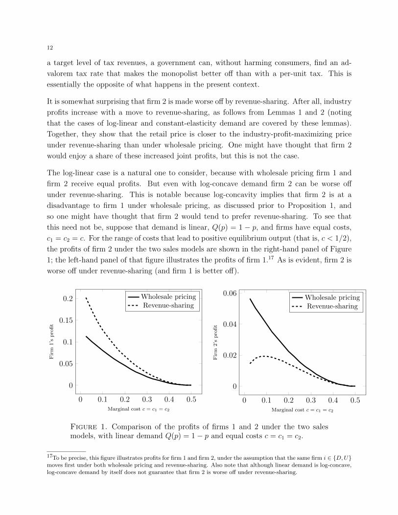
this need not be, suppose that demand is linear, Q(p) = 1 − p, and firms have equal costs,

c1 = c2 = c. For the range of costs that lead to positive equilibrium output (that is, c < 1/2),

the profits of firm 2 under the two sales models are shown in the right-hand panel of Figure

1; the left-hand panel of that figure illustrates the profits of firm 1.17 As is evident, firm 2 is

worse off under revenue-sharing (and firm 1 is better off).

0 0.1 0.2 0.3 0.4 0.5

0

0.05

0.1

0.15

0.2

Marginal cost c = c1 = c2

Fir

m1’s

pro

fit

Wholesale pricingRevenue-sharing

0 0.1 0.2 0.3 0.4 0.5

0

0.02

0.04

0.06

Marginal cost c = c1 = c2

Fir

m2’s

pro

fit

Wholesale pricingRevenue-sharing

Figure 1. Comparison of the profits of firms 1 and 2 under the two salesmodels, with linear demand Q(p) = 1− p and equal costs c = c1 = c2.

17To be precise, this figure illustrates profits for firm 1 and firm 2, under the assumption that the same firm i ∈ {D,U}moves first under both wholesale pricing and revenue-sharing. Also note that although linear demand is log-concave,log-concave demand by itself does not guarantee that firm 2 is worse off under revenue-sharing.

13

However, for other log-concave demand functions, firm 2 is better off under revenue-sharing—

it benefits from the increase in overall demand brought about by the retail price reduction

that occurs under the move to revenue-sharing. For example, when the underlying consumer

valuations are distributed according to a beta distribution with parameters ν = 3 and ω = 1,

it can be shown that firm 2 is better off with revenue-sharing.18 Indeed, at these parameters

the underlying density function is log-concave, which implies that the induced demand func-

tion is log-concave. Thus, Proposition 2 does not fully generalize to all log-concave demand

or even to all demand generated from log-concave density functions. However, as I show in

Proposition 3 below, when considering both a shift to revenue-sharing and a change in the

order in which firms move, the results do generalize.

At a slightly technical level, insight into Proposition 2 and its limitations is provided by

considering log-linear demand. In this case, it can be shown that even if firm 2 chose the

price pa (that would obtain under revenue-sharing) when wholesale pricing is in effect, its

resulting margin would be higher than it is under revenue-sharing (in which the same price pa

is the equilibrium outcome). This means firm 2, even behaving suboptimally under wholesale

pricing, could obtain a higher margin under wholesale pricing than it does behaving optimally

under revenue-sharing. Because it would sell the same number of units in either case, it

must prefer wholesale pricing. For this approach with log-linear demand, the fact that the

markup that firm 1 would choose under wholesale pricing is given by λ(pw)(1− λ′(pw)) = λ

(a constant) greatly simplifies the comparison with revenue-sharing. That is, under more

general demand the markup that firm 1 would choose under wholesale pricing need not be

readily comparable to that under revenue-sharing and indeed as mentioned the result need

not hold for certain demand functions.

So far my discussion and results have centered on the preferences of market players over

changes in either the move order (whether they set retail prices or terms of trade) or whether

revenue-sharing or instead wholesale prices are used. However, it is of interest to know how

players evaluate a change in both the move order and the mechanism by which surplus

is transferred. The reason is that recently there have been many real-world markets that

have undergone a change from the wholesale model to the agency model. Recall that this

corresponds to moving from a situation where firm U sets w and D then sets p to a situation

where D sets r and U then sets p.

Proposition 3. If demand is log-concave, log-linear, or constant-elasticity, then a shift from

the wholesale model to the agency model raises the profits of D but lowers the profits of U .

18The density function of the beta distribution with parameters ν and ω evaluated at x is given by

xν−1(1− x)ω−1

B(ν, ω)

where B(ν, ω) is the beta function. For a broad range of symmetric costs that I simulated, firm 2 was always betteroff with revenue-sharing.

14

From a practical standpoint, Proposition 3, along with its generalization to bilateral imper-

fect competition in the next section, provides a potential explanation for why online firms

such as Amazon and eBay may be switching to the agency model, and also of course suggests

suppliers need not be beneficiaries of this change. This presumes, of course, that the demand

curves in those markets are reasonably approximated by those covered by Proposition 3.19

The most interesting cases are where there are conflicting forces from the combination of

change in move order and change in business model. For example, continuing to maintain

the focus on retailers, consider D, suppose demand is constant-elasticity and that initially

the wholesale model is in place. Then (from the discussion prior to Proposition 1), D earns

higher profits than U does, and so a shift in only the move order would make D worse off.

However, as the current proposition shows, completing the move to the agency model by

also imposing revenue-sharing would make D better off than it was originally. Thus, the

overall intuition for this result is that the advantage of revenue-sharing for the firm setting

the terms of trade is so strong that it overwhelms any other effect. This resonates well with

my earlier result that under revenue-sharing it is always advantageous to set the terms of

trade (Proposition 1).

2. Bilateral Imperfect Competition

In this section I extend the model and analysis above to a setting in which there is imperfect

competition at both layers of the supply chain.20 Rather than specify any particular model

of such competition, I take an approach based on conduct parameters similar to that in the

study of pass-through under wholesale pricing by Weyl and Fabinger (2013), and which is

related to work by Gaudin and White (2014b).21 This allows my results to be stated in

terms of properties of the aggregate demand function in the industry, thus providing a close

analogue to the study of bilateral monopoly above.

2.1. A conduct-parameter approach. Given the work above, it is easier here to adopt an

approach that is slightly more compact. Let Q(p) denote the aggregate demand of consumers,

where one interpretation is that there are multiple substitute products each sold at common

price p, that there are multiple substitute retailers, and that demand is symmetric at p. As

before, λ(p) = −Q(p)/Q′(p). All derivatives in this section measure the effect of an increase

19Note also that all of the demand cases covered by this proposition are also covered by Lemma 2.20Related work that considers market power at multiple stages of production includes Salinger (1988), Reisinger andSchnitzer (2012), and Kourandi and Vettas (2012).21In an earlier draft of this paper, I specified a complete micro-foundation for such competition, and showed thatmoving from the wholesale model to the agency model could lower retail prices yet also make the downstream firmsbetter off at the expense of upstream firms. A downside of that model was that only very limited forms of demandcould tractably be considered. In particular, that model effectively assumed pass-through rates equal to unity.

15

in the common price p of the retail prices of all products sold through all stores. Thus, Q′(p)

measures the effect on aggregate demand from a small increase in all prices.

My analysis proceeds as follows. First, I specify how layer 2 reacts to arbitrary terms of

trade r or w, that is, which retail price p is set by the second layer given such terms of trade.

Second, I specify how the first layer determines these terms of trade, taking as given the

response of the second layer.

Suppose that (symmetric) terms of trade have been set by the first layer: all firms offering

contracts offer either the same revenue share r or the same wholesale price w. Let m2(p)

denote the per-unit margin of the second layer, given that all firms of that layer are setting

the same price p. Under wholesale pricing m2(p) = p−w−c2 whereas under revenue-sharing

m2(p) = rp− c2. The aggregate profit of the second layer is m2(p)Q(p), with derivative

m′2(p)Q(p) +m2(p)Q′(p).

For arbitrary r or w, I define the value of p set by layer 2 to be that which implicitly solves

m2(p)

m′2(p)= θ2λ(p) =⇒ m2(p) = θ2m

′2(p)λ(p), (7)

where θ2 ∈ (0, 1) is an exogenous constant that represents the conduct parameter of layer 2.

Computing the appropriate derivatives m′2(p), under wholesale pricing this says that m2(p) =

p − w − c2 = θ2λ(p) whereas under revenue-sharing (and using m′2(p) = r) this says that

m2(p) = rp− c2 = rθ2λ(p).

Note that if θ2 = 1 then these equations are precisely what was derived earlier for the optimal

response of firm 2 in the case of bilateral monopoly (see Equations (1) and (3)). On the other

hand, if θ2 = 0 then these margins are zero. Thus, varying θ2 spans the range of outcomes

from perfect competition in layer 2 to perfectly collusive behavior in layer 2.22

Now consider the profits of layer 1. As before, it can be supposed that this layer sets p, with

the terms of trade with layer 2 then equilibrating. For any final price p, the per-unit margin

of layer 1 is denoted by m1(p), and satisfies

m1(p) = p− c1 − c2 − m2(p), (8)

where m2(p) is the margin that layer 2 must be receiving if p is the price layer 2 selects.

From the work above, for a given p the margin of the second layer is m2(p) = θ2λ(p) under

wholesale pricing. Under revenue-sharing this margin is rθ2λ(p), but using the equilibrium

condition given just above for layer 2 (that rp− c2 = θ2rλ(p)), r is given by

r =c2

p− θ2λ(p),

22In line with assumptions from the analysis of bilateral monopoly, I suppose that the right-hand side of Equation (7)intersects the left-hand side once and from above, and that layer 2’s profits are quasiconcave in p for any given termsof trade.

16

a close analogue to Equation (4). Thus eliminating r, under revenue-sharing

m2(p) =θ2c2λ(p)

p− θ2λ(p). (9)

For arbitrary p, the overall profitability of the first layer is simply m1(p)Q(p), with derivative

m′1(p)Q(p) +m1(p)Q′(p).

I define the equilibrium value of p to be that which satisfies

m1(p)

m′1(p)= θ1λ(p) =⇒ m1(p) = θ1m

′1(p)λ(p), (10)

where θ1 ∈ (0, 1) is an exogenous constant that represents the conduct parameter of layer 1.

As θ1 ranges from zero to one the resulting price p ranges from that which gives layer 1 no

margin to that which maximizes the profits of layer 1 (given how layer 2 will respond).23

Noting that m′1(p) = 1−m′2(p) (using Equation (8)) and computing the value of m′2(p) under

both wholesale pricing and revenue-sharing, equations characterizing the industry price are

readily derived. As before, let pw and pa denote the equilibrium retail prices when wholesale

prices or instead revenue-sharing is used.

Lemma 3. Under bilateral imperfect competition with conduct parameters θ1 and θ2, the

retail price pw under wholesale pricing satisfies

pw − c1 − c2 = θ2λ(pw) + θ1λ(pw)(1− θ2λ′(pw)), (11)

and the retail price pa under revenue-sharing satisfies

pa − c1 − c2 = θ1λ(pa) + θ2c2λ(pa)

[pa(1− θ1λ

′(pa)) + λ(pa)(θ1 − θ2)

(pa − θ2λ(pa))2

]. (12)

If θ1 = θ2 = 1, these equations reduce to those derived for the bilateral monopoly case

(Equations (2) and (6)). And, for θ1 = θ2 = 0, both of these industry margins equal zero.

Finally, note that pw is, once again, independent of which firm moves first, as can be seen

by expanding the right-hand side of Equation (11).

I will now show that, under broadly similar conditions on the shape of demand, key results

derived for bilateral monopoly continue to hold under bilateral imperfect competition. I

begin by investigating the desire of D or U to move first when revenue-sharing is in effect.

Denote by θD and θU the underlying conduct parameters of the two layers.

Proposition 4. Under revenue-sharing, each firm prefers to be the first-mover if either of

the following conditions hold:

23In line with assumptions from the analysis of bilateral monopoly, I suppose that the right-hand side of Equation(10) intersects the left-hand side once and from above (in the range where p > c2 + θ2λ(p)), and that layer 1’s profitsare quasiconcave in p.

17

(1) market power is balanced (θD = θU),

(2) aggregate demand Q(p) is log-linear or constant elasticity.

This proposition confirms that moving first under revenue-sharing is particularly appealing

under bilateral imperfect competition. The intuition is clearest when market power is bal-

anced. In that case, although the logic is more involved than in the bilateral monopoly case,

a conceptually similar argument can be made. Loosely speaking, it can be shown that the

first-mover can replicate the retail price that would emerge if it were instead the second-

mover.24 Although doing so is suboptimal, it is possible and moreover would lead to the

same number of units being sold. Similar to the earlier result, it is then possible to explicitly

show that charging this lower price would enable the first-mover to ensure itself a higher

share of revenues than it receives as a second-mover. Thus, the first-mover can ensure itself

a higher margin than it gets when it is the second-mover (while also selling as many units

as it sells as the second-mover).

The next question is what happens to the retail price when revenue-sharing is in effect.

Lemma 4. Under bilateral imperfect competition, if the elasticity of Mills ratio is less than

one (pλ′(p)/λ(p) ≤ 1), then the equilibrium retail price under revenue-sharing is strictly less

than that under wholesale pricing (pa < pw). This result holds even if the move order differs

depending on whether wholesale pricing or revenue-sharing is used.

In prior work, Gaudin and White (2014b) independently derive this result for the case where

there is an upstream monopolist (represented by a government maximizing tax revenues).

I extend their result by showing that even when there is competition at both layers of the

supply chain, and regardless of which layer sets the retail price, revenue-sharing tends to

lower prices.25

However, there is an important qualitative difference compared to the case of bilateral mo-

nopoly or upstream monopoly (as considered by Gaudin and White (2014b)). Recall that in

the bilateral monopoly case a move to revenue-sharing lowers the retail price, which moves

it closer to the price that maximizes industry profits. In contrast, with bilateral imperfect

competition a price reduction starting from pw may lower industry profits. The reason is

simply that, depending on the conduct parameters, pw may be lower than the price that

maximizes industry profits, so that a further price reduction further lowers industry profits.

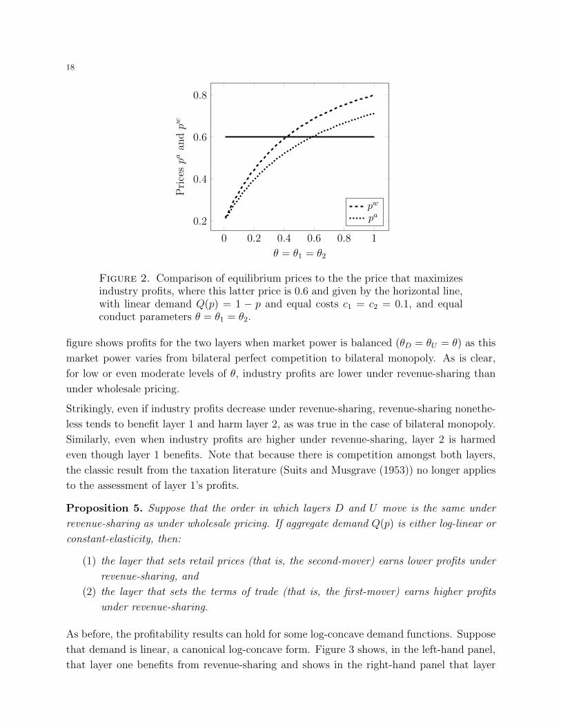
This possibility can be seen clearly in Figure 2, which graphs equilibrium prices in compar-

ison to the price that maximizes industry profits for a linear-demand specification. That

24The description here is loose in that the layers are compelled to pick prices that satisfy the conditions above, ratherthan being free to select arbitrary prices. See the proof for details.25Anderson et al. (2001) show a related result, which is that a government can always raise as much revenue andreach higher output under an ad-valorem tax rather than a unit tax, when selling to competing downstream firms.However, they do not consider the case where the government seeks to maximize revenue.

18

0 0.2 0.4 0.6 0.8 1

0.2

0.4

0.6

0.8

θ = θ1 = θ2

Pri

cespa

andpw

pw

pa

Figure 2. Comparison of equilibrium prices to the the price that maximizesindustry profits, where this latter price is 0.6 and given by the horizontal line,with linear demand Q(p) = 1 − p and equal costs c1 = c2 = 0.1, and equalconduct parameters θ = θ1 = θ2.

figure shows profits for the two layers when market power is balanced (θD = θU = θ) as this

market power varies from bilateral perfect competition to bilateral monopoly. As is clear,

for low or even moderate levels of θ, industry profits are lower under revenue-sharing than

under wholesale pricing.

Strikingly, even if industry profits decrease under revenue-sharing, revenue-sharing nonethe-

less tends to benefit layer 1 and harm layer 2, as was true in the case of bilateral monopoly.

Similarly, even when industry profits are higher under revenue-sharing, layer 2 is harmed

even though layer 1 benefits. Note that because there is competition amongst both layers,

the classic result from the taxation literature (Suits and Musgrave (1953)) no longer applies

to the assessment of layer 1’s profits.

Proposition 5. Suppose that the order in which layers D and U move is the same under

revenue-sharing as under wholesale pricing. If aggregate demand Q(p) is either log-linear or

constant-elasticity, then:

(1) the layer that sets retail prices (that is, the second-mover) earns lower profits under

revenue-sharing, and

(2) the layer that sets the terms of trade (that is, the first-mover) earns higher profits

under revenue-sharing.

As before, the profitability results can hold for some log-concave demand functions. Suppose

that demand is linear, a canonical log-concave form. Figure 3 shows, in the left-hand panel,

that layer one benefits from revenue-sharing and shows in the right-hand panel that layer

19

two is worse off. Indeed, the decline in profits for layer 2 can be quite dramatic, in some

cases being roughly one-third under revenue-sharing what they are with wholesale pricing.

0 0.2 0.4 0.6 0.8 10

0.05

0.1

Conduct parameter θ = θ1 = θ2

Layer

1’s

pro

fit

Wholesale pricingRevenue-sharing

0 0.2 0.4 0.6 0.8 1

0

0.02

0.04

0.06

Conduct parameter θ = θ1 = θ2L

ayer

2’s

pro

fit

Wholesale pricingRevenue-sharing

Figure 3. Comparison of the profits of industry layers 1 and 2 under whole-sale pricing and revenue-sharing, with linear demand Q(p) = 1−p, equal costsc = c1 = c2 = 0.1, and equal conduct parameters θ = θ1 = θ2.

I now consider a shift from the wholesale model to the agency model. The following result

extends Proposition 3, and explains what happens to the profits of the two layers starting

from the wholesale pricing model in which layer U sets w and then layer D sets p, and

moving to the revenue-sharing model in which layer D sets r and then layer U sets p.

Proposition 6. Under bilateral imperfect competition, if demand is log-concave, log-linear,

or constant-elasticity, then a shift from the wholesale model to the agency model raises the

profits of layer D but lowers the profits of layer U .

2.2. Robustness. The conduct-parameter approach used above has several attractive fea-

tures. First, it allows for a parsimonious representation of bilateral imperfect competition

that is easy to work with both under wholesale pricing and revenue-sharing. Second, the

shape of aggregate demand is central to the analysis, thus providing a close analogue to the

study of bilateral monopoly.

At the same time, the approach above utilizes several strong assumptions. For example,

if static competition in prices between firms offering differentiated products is taken as a

microfoundation, then the conduct parameters may depend on the shape of demand at any

given price rather than being constants. Additionally, the conduct parameter of the layer

that moves first may depend on whether wholesale prices or instead revenue-sharing is used

(although the conduct parameter of the layer that moves second is invariant to this).

20

To investigate whether my results are particularly sensitive, I consider a particular micro-

foundation. Suppose there are two suppliers and two retailers, where each supplier sells

to one retailer—competition occurs across vertical chains. The demand for a given retailer

setting a price p while its rival retailer sets a price p is given by

Q(p, p) =1− β − p+ βp

1− β= 1− p− βp

1− β, for β ∈ [0, 1).

As β becomes close to one the market becomes very competitive and for β = 0 the retailers

are monopolists. The four firms have identical marginal costs c > 0. Contract offers are

private so that, for example, if suppliers move first then they privately offer either a wholesale

price or a revenue share to their downstream partner, which then sets a retail price.

It can be shown that this microfoundation leads to a conduct parameter for the first-mover

that depends on whether revenue-sharing or instead wholesale pricing is in effect. Does this

overturn my earlier results? The equilibrium values are readily computed for different values

of c and β. For a broad range of parameters that I considered, my key results from above

typically, although not always, hold.26

In particular, I found that (i) the equilibrium price under revenue-sharing was always lower

than under wholesale pricing, (ii) the firms that set retail prices were always harmed by a

move to revenue-sharing, but that (iii) when β was large (typically, exceeding 0.8), so that

the market is very competitive and profits are close to zero, the firms that move first could

be worse off under revenue-sharing. Despite (iii), I found that (iv) a move from the wholesale

model to the agency model always benefited downstream firms and harmed upstream firms.

Finally, (v) under revenue-sharing it was always advantageous to move first. Of the five

items above, only (iii) diverges from my theoretical predictions under the conduct-parameter

approach, and then only for extreme parameter values.

3. Most-Favored Nation Clauses

In this section I explore the use of retail price-parity clauses such as MFN clauses. Such

clauses specify that a supplier who is setting retail prices through one retailer cannot charge

a lower price through another retailer, if the first has an MFN clause. Such clauses are

growing in popularity, especially in online markets, and so understanding their effects is

important.27 I show how price-parity clauses can raise retail prices and harm consumers. I

26I let β vary between zero and 0.95 in increments of 0.05, and considered a variety of costs from 0.01 to 0.45(production is only positive for c ≤ 0.5).27One reason for their popularity is likely that violations of such clauses can be detected because retail prices aretypically easily observable, especially relative to more traditional wholesale MFN contracts that stipulate parity inwholesale prices. See Baker (1996) for a broad discussion of such contracts. Also see McAfee and Schwartz (1994)and DeGraba and Postlewaite (1992) for assessments of the ability of such contracts do limit expropriation resultingfrom a supplier’s inability to commit in multilateral negotiations.

21

also describe examples of online agency markets where price-parity clauses have been used.

In the conclusion, I discuss potential pro-competitive effects of such clauses.

Rather than using an approach based on exogenous conduct parameters, I adopt specific

microfoundations. Otherwise, I would have to assume that, for example, price-parity clauses

increase the conduct parameter of certain firms and thereby raise prices. Instead, I will

directly prove that such contracts have the effect of raising prices.

3.1. Retail price-parity clauses raise industry prices. To investigate retail price-parity

clauses, I assume throughout this section that retailers set terms of trade and suppliers set

retail prices. The basic argument for why such clauses raise industry prices is that they

soften competition in the terms of trade between retailers, leading retailers to charge higher

commissions. By effectively raising the costs faced by suppliers, such clauses in turn lead to

higher equilibrium retail prices.

The intuition for why price-parity restrictions soften competition between retailers setting

the terms of trade is as follows. In the absence of such clauses, when a retailer raises

the commission that it charges upstream firms, those upstream firms have incentives to

adjust both the retail price they set at that retailer and the retail price they set at other

retailers. Indeed, suppliers have an incentive to adjust these prices asymmetrically, so that

demand is diverted away from the retailer that has raised its commission. This disciplines

the retailer in question, reducing its incentives to raise commissions. However, price-parity

clauses eliminate the ability of suppliers to divert demand in such a manner, so that such

clauses encourage retailers to raise their commissions.

To build intuition and emphasize the basic technique involved, first I focus on a special case

in which each retailer carries but a single supplier’s product, in which contracts offered by

retailers are privately observed, and in which wholesale pricing is used. Afterwards, I explain

how to generalize.

3.1.1. Price-parity restrictions with exclusive retailers, private contracts, and wholesale pric-

ing. Here I consider a static price-setting model with symmetrically differentiated products

and in which wholesale pricing is used. There are two upstream firms and four downstream

firms. Each upstream firm sells to two downstream firms, each of which is exclusive to a

single upstream firm. Contract offers are private.28

Suppose no MFNs are in effect and consider a given supplier. This supplier is selling its

product through two exclusive retailers. Facing a commission of w from one retailer and w

from the other, this supplier chooses retail prices of p and p, respectively. Let Q(p, p, p, p)

denote the quantity it sells through a downstream retailer given that it charges p at that

28Because each retailer only offers a contract to one supplier, I assume that a supplier who receives an unexpectedoffer from a retailer does not adjust its beliefs about any other offers.

22

retailer and p at the other retailer through which it sells, and given that the other supplier

charges p at each of the two retailers to which it sells. Demand is symmetric across retailers

and satisfies all of the usual properties of differentiated product demand.29 The profits of

the supplier under consideration are

(p− w − cU)Q(p, p, p, p) + (p− w − cU)Q(p, p, p, p). (13)

At a symmetric industry solution, all retailers are setting the same wholesale price w and all

suppliers are setting the same price p through all retailers. As verified in the Appendix, for

such an arbitrary (industry-wide) w, this gives an industry-wide price p characterized by

p− w − cU = − Q(p)

Q1(p) +Q2(p), (14)

where Q(p) is defined as Q(p) = Q(p, p, p, p), and similarly Q1(p) = Q1(p, p, p, p) and

Q2(p) = Q2(p, p, p, p) (note that Q1 6= Q2).30 As I show in the Appendix, this same equation

characterizes the industry-wide price p that would be chosen by suppliers facing an industry-

wide w if MFNs were in effect across the industry. The intuition is simply that, if all retailers

are charging the same wholesale price w, then from the perspective of suppliers it doesn’t

matter if MFNs are in effect or not—suppliers have no incentive to charge asymmetric retail

prices when they face symmetric wholesale prices.

In line with earlier analysis, I assume that the right-hand side of Equation (14) intersects the

left-hand side only once and from above. Let p∗(w) denote the solution to Equation (14),

so that p∗(w) gives the industry-wide retail price that holds given that the industry-wide

wholesale price is w, whether MFNs are in effect or not. Note that p∗(w) is increasing.

I now consider the decisions of retailers. For clarity I reiterate that, for a given retailer,

Q(p, p, p, p) is the demand facing this retailer given that its supplier charges a price p through

it and charges a price p through the other retailer carrying its product, and given that p

is charged by the other supplier through both of its retailers. If this retailer is charging a

wholesale price w, its profits are (w − cD)Q(p, p, p, p). Because contracts are private, when

this retailer selects w only the prices chosen by this retailer’s supplier, p and p, change—that

is, the prices set by the other supplier, given by p, do not change. Nonetheless, both p and

p and their derivatives with respect to this retailer’s wholesale price w are also functions

of the wholesale price w charged by the other retailer carrying this supplier’s product and

of the retail price p set for the other supplier’s product through its retailers. I will thus

29Throughout I assume that the demand system is well-behaved. First-order conditions will uniquely characterizesymmetric equilibrium outcomes, and any needed second-order conditions are satisfied (for example, marginal profitswith respect to any choice variable are decreasing in that choice variable).30The reason that Q1 6= Q2 is that Q1 denotes the change in the demand at a given retailer when its supplier raisesthe price set at that retailer, whereas Q2 is the change in the demand at this retailer when its supplier raises theprice it sets at the other retailer to which it sells.

23

write p(w, w, p, p) and p(w, w, p, p), and write p1(w, w, p, p) and p1(w, w, p, p) to denote the

derivatives with respect to the first argument w.

With no MFNs, the first-order condition governing this retailer’s choice of w is

Q(p, p, p, p) + (w − cD) [Q1(p, p, p, p)p1(w, w, p, p) +Q2(p, p, p, p)p1(w, w, p, p)] = 0. (15)

To be clear, for a retailer that raises its wholesale price w slightly, p1 is the change in the

price set at its own store by its supplier and p1 is the change in the price set through the

other store to which this retailer’s supplier sells. Thus, for this retailer, Q1p1 + Q2p1 is

the total change in demand following an increase in its wholesale price, factoring in how its

supplier will change the price that it charges through its two retailers.

At a symmetric industry solution where all retailers set the same wholesale price w and all

suppliers set the same price p∗(w) through all retailers, the following holds.

w − cD = − Q(p∗(w))

Q1(p∗(w))p1(w,w, p∗(w), p∗(w)) +Q2(p∗(w))p1(w,w, p∗(w), p∗(w)). (16)

Now suppose price-parity is in effect across the industry. This retailer’s profit function differs

in that its supplier must charge the same price pM(w, w, p, p) through both retailers it sells

to, meaning this retailer’s profits are (w− cD)Q(pM , pM , p, p), where pM is a function of the

same variables that p and p are functions of. Differentiating and looking for a symmetric

industry-wide solution in which all retailers set w and all suppliers charge p∗(w) through all

their retailers, the following industry-equilibrium condition holds.31

w − cD = − Q(p∗(w))

Q1(p∗(w))pM1 (w,w, p∗(w), p∗(w)) +Q2(p∗(w))pM1 (w,w, p∗(w), p∗(w)). (17)

The effect of industry-wide price-parity restrictions on the equilibrium wholesale price de-

pends on how the solution to Equation (16) differs from the solution to Equation (17).

Inspecting these equations, it is apparent that these differ to the extent that pM1 differs from

p1 and p1, that is in how such restrictions influence the retail price response of suppliers

to changes in the wholesale price charged by a single retailer. As I show in the Appendix,

p1 > pM1 > p1. This says that price-parity restrictions force a supplier, responding to a

wholesale price change by a single retailer, to compress what its price responses otherwise

would be, which has the effect of causing such a wholesale price increase to result in less de-

mand being diverted from the a retailer raising its wholesale price. This encourages retailers

to raise their wholesale prices, which in equilibrium raises the retail price.

Proposition 7. In the model with exclusive retailers and private contracts, industry-wide

retail price-parity restrictions lead to an increase in retail prices.

31In line with earlier analysis, I assume that the right-hand side of both Equations (16) and (17) intersects theleft-hand side only once, and from above, as the industry-wide wholesale price changes.

24

3.1.2. Price-parity restrictions with multi-product retailers and public contracts. I now gen-

eralize Proposition 7 in a setting with a total of two suppliers and a total of two retailers.

In particular, I show the result is robust to (i) allowing each of two retailers to carry the

products of both suppliers, (ii) allowing public rather than private contracts, (iii) allowing

for either revenue-sharing or wholesale pricing.

It is necessary to introduce slightly different notation. Label the suppliers as 1 and 2, and

the two (in total) retailers as A and B. Let p1 and p2 denote the prices charged at retailer A

by suppliers 1 and 2, respectively, and let p1 and p2 denote the prices charged at retailer B

by suppliers 1 and 2, respectively. Let Π(p1, p1, p2, p2) denote the profits of supplier 1, given

whatever terms of trade suppliers face. Additionally, denote the demand for this supplier’s

good at retailer A by Q(p1, p1, p2, p2). As before, the demand system is symmetric.

The situation is somewhat more complicated than before because the price-adjustment pro-

cess of suppliers (in response to the change in a single retailer’s contract) must capture the

overall strategic adjustment of all suppliers’ prices. That is, because contracts are public,

and also because each supplier sells to each retailer, any change in a single retailer’s contract

will alter all the retail prices.

Given symmetry, it is enough to think about retailer A raising either its wholesale price w or

revenue-share r to both suppliers 1 and 2 (depending on whether wholesale prices or instead

revenue-sharing is in effect), given that retailer B is either offering w or r to both suppliers.

Given that suppliers will behave symmetrically given such terms of trade, it will be that

p1 = p2 (both suppliers set the same price at retailer A) and that p1 = p2 (both suppliers

set the same price at retailer B). When wholesale prices are in effect, denote by p(w, w) this

common price set through A (so that p = p1 = p2) and denote by p(w, w) this common price

set through B (so that p = p1 = p2). In an abuse of notation, when revenue-sharing is in

effect I will also denote these prices by p and p, although their arguments are r and r.32

The key to understanding the effect of price-parity restrictions is understanding how they

influence retail price adjustments in response to a change in a single retailer’s terms of trade.

Hence, let p1(w, w) denote the change in the price p(w, w) (that both supplier 1 and 2

charge through retailer A), let p1(w, w) denote the change in the price p(w, w) (that both

suppliers set through retailer B), and let pM1 (w, w) denote the common change in all retail

prices when price parity is in effect, all in response to an increase in the wholesale price w

offered by A to both suppliers. In an abuse of notation, when revenue-sharing is in effect

I let p1(r, r), p1(r, r), and pM1 (r, r) denote the changes in these prices in response to a small

increase in r by retailer A.

32In particular, the function p under wholesale pricing is different from the function p under revenue-sharing, andthe same is true for p.

25

A sufficient condition for price-parity clauses to raise prices is that when a retailer offers

terms that are more advantageous to suppliers, suppliers do not change prices in a way that

diverts demand to the retailer’s rival. For the case of wholesale prices, this is equivalent to

a retailer losing demand if it raises its wholesale price, and this is most conveniently written

as p1 > p1: when retailer A raises its wholesale price, suppliers respond by raising the retail

price at A by more than the retail price is raised at retailer B. Under revenue-sharing,

an increase in r will tend to lower prices by lowering the perceived marginal costs cU/r of

suppliers. Thus, the relevant sufficient condition is that p1 < p1: a retailer who gives a

supplier a larger share of revenue causes a price decrease at its own store that dominates

any price decrease at the other retailer.

Proposition 8. Consider the model with public contracts in which each of two suppliers

sells through each of two retailers. Suppose that, when a retailer offers better terms to its

suppliers, the corresponding price effects do not divert demand to the retailer’s rival. That

is, suppose it is the case that p1 > p1 (under wholesale pricing) or that p1 < p1 (under

revenue-sharing). Then industry-wide retail price-parity restrictions increase retail prices.

The conditions to ensure that, for example, p1 > p1 can readily be stated in terms of stability

conditions for the underlying profit functions of suppliers. In particular, using the work in

the proofs of Propositions 7 and 8, at a symmetric equilibrium (w = w and all retail prices

equal), p1 and p1 are readily derived in terms of partial derivatives of a supplier’s profit

function. Roughly speaking, so long as a supplier’s marginal profits from increasing its price

at a given retailer are more strongly influenced by price changes at that retailer than at the

other retailer, and so long as an increase in all prices tends to lower the marginal gains from

a price increase at a given retailer, then p1 > p1 (under wholesale pricing).33

3.2. Antitrust cases. In this section I describe markets in which retail price-parity clauses,

used in conjunction with the agency model, were investigated by antitrust authorities either

in the EU or the US or both. In all cases, a key concern of authorities was that higher retail

prices either could or did result.

33In particular, let Π represent the profits of, say, supplier 1. Then

p1 =[Πp1p1 + Πp1p2 ]Q1 − [Πp1p1 + Πp1p2 ]Q2

[Πp1p1 + Πp1p2 ]2 − [Πp1p1 + Πp1p2 ]2, and p1 =

[Πp1p1 + Πp1p2 ]Q2 − [Πp1p1 + Πp1p2 ]Q1

[Πp1p1 + Πp1p2 ]2 − [Πp1p1 + Πp1p2 ]2.

Because Q1 < 0 < Q2 and Q1 is larger in magnitude than Q2, the following stability-type conditions ensure p1 > p1,evaluated at equal wholesale and retail prices. First, [Πp1p1 + Πp1p2 ]2 − [Πp1p1 + Πp1p2 ]2 > 0. Second, [Πp1p1 +Πp1p2 ] + [Πp1p1 + Πp1p2 ] < 0. To interpret these, note that Πp1 is the marginal profitability of supplier 1 increasingits price at retailer A. The first condition basically says that the magnitude of the effect on this marginal profitabilityfrom an increase in both suppliers’ prices at this retailer (given by p1 and p2) dominates the effect from an increasein both suppliers’ prices at the other retailer (given by p1 and p2). The second condition ensures that the overalleffect of increasing all of these prices is to reduce the marginal profitability of an increase in p1; in this sense, thesecond condition is similar to the assumption of concave profits in a monopoly pricing problem.

26

The Amazon Marketplace is an online sales platform implemented by Amazon which covers

a wide variety of products and accounts for over 40% of products sold by Amazon.34 Amazon

sets a revenue-sharing contract and suppliers set the retail price that consumers see when they

visit Amazon’s website, sharing with Amazon revenue from completed sales. Additionally,

Amazon has used price-parity clauses.

Both the Bundeskartellamt (Germany’s antitrust agency) and the UK’s Office of Fair Trade

(OFT) investigated Amazon’s use of such clauses. The concern was essentially as outlined

in my analysis above.35 Amazon agreed to stop using such clauses in the affected markets.

The OFT also investigated the use of MFN contracts in the private motor insurance market.

In that market, private motor insurers (PMIs) set the price of their products sold through

price-comparison websites (PCWs) and MFN clauses are used. In its Provisional Findings

Report (December 17, 2013), the OFT provides much the same argument that I have made

above, in particular that MFNs stifle competition in commissions by PCWs, ultimately

leading to higher retail prices. They also present direct evidence that such clauses limit

commission competition.36

Another investigated market is that for online hotel room booking. Leading online travel

agencies such as Expedia and Booking.com take a share of revenue from bookings of rooms

on their websites, where the prices are set by the owners of the hotel rooms. However, there is

some scope for websites to discount offerings, for example by bundling hotel rooms with other

travel-related products and offering an advantageous price on the bundle. Both Expedia and

Booking.com imposed a combination of MFN clauses and resale price maintenance (RPM)

agreements on upstream suppliers. Both the OFT and its French counterpart, The General

Directorate for Competition Policy, Consumer Affairs and Fraud Control, have expressed

concerns about the contractual provisions used by the booking firms (in the US, a private

lawsuit is currently underway).37 As part of an agreement reached in January, 2014, these

firms agreed to stop using such contracts in the UK. However, this agreement was later

overturned and the case was closed on the grounds of administrative priorities.38

The most closely watched market was that for e-books. In 2010, Apple entered the e-book

market as it introduced its tablet computer, the iPad. Prior to Apple’s entry, Amazon was

34See “OFT minded to drop investigation into Amazon pricing policies,” Financial Times, August 29, 2013.35In an August 29, 2013 announcement, the OFT noted the primary concern related to such clauses, saying, “Inparticular, such policies may raise online platform fees, curtail the entry of potential entrants, and directly affect theprices which sellers set on platforms (including their own websites), resulting in higher prices to consumers.”36The report reads, “There is direct evidence that wide MFNs harm competition between PCWs. Notably, one PCWhas tried to reduce its commission fees with motor insurance providers in exchange for lower premiums. However,motor insurance providers were unable to accept the offer due to the presence of wide MFNs in their contracts withother PCWs. A number of motor insurers also told us they had, as a result of wide MFNs, withdrawn from, or didnot consider, such offers from PCWs.”37See, for example, “Expedia, Starwood Ask Judge to Dismiss Price-Fixing Suit,” Bloomberg, December 17, 2013.38In France, specifically for hotel bookings, MFNs of all types (including both so-called narrow and wide MFNs) havebeen banned. Germany has banned all MFNs, not only those affecting hotel bookings.

27

the the only significant player in the market, selling e-books for its dedicated e-book reader,

the Kindle.

Publishers had been unhappy dealing exclusively with Amazon. One reason is that they

thought Amazon’s pricing was contributing to the decline of profits from other formats and

channels, such as hardcover and paperback books sold through brick and mortar retailers.

Apple convinced publishers to adopt the agency model as a condition of its entry into e-

book retailing, and publishers then pressured Amazon to do so as well. Apple also secured

an MFN contract for itself prior to entering. Following Apple’s entry, the price of many

e-books significantly increased.

In April, 2012, the US Department of Justice accused Apple and five major publishers of

conspiring to increase the price of e-books, and a similar investigation began in the EU.

Propositions 7 and 8 predict this increase in retail prices.39 Indeed, the price increase caused

by MFNs under the agency model may be sufficient to outweigh the price decrease that is

predicted to occur from the shift to the agency model from the wholesale model. That is, it

is MFNs not the agency model itself that may have caused the increase in prices.

4. Conclusion

I have presented an analysis of vertical relations in markets where there may be imperfect

competition at both layers of the supply chain. The model is general enough to allow for

changes in which layer sets retail prices and for either wholesale prices or instead revenue-

sharing to be used to intermediate trade. I also examined retail price-parity restrictions.

The broad message from my analysis is that revenue-sharing, the agency model, and retail

price-parity clauses are weapons that firms can use to either shift profits across the supply

chain or to raise retail prices. A move to revenue-sharing tends to raise the profits of the

firms setting terms of trade, while the profits of other firms tend to decrease. Consumers

are better off, at least in the absence of price-parity restrictions. This result is strengthened

when a switch from the wholesale model to the agency model is considered, so that retailer

profits increase but supplier profits fall. Price-parity restrictions, when imposed within the

agency model, raise prices and may erase the gains that otherwise would have accrued to

consumers from the agency model being in place instead of the wholesale model.

Although the analysis above indicates how MFNs may raise prices and harm consumers, it

is not hard to imagine how MFNs might also be pro-competitive. For example, MFNs might

39A potential criticism of this interpretation hinges on the question of whether revenue-sharing contracts raise pro-ducers’ perceived marginal costs in the e-book market, given that one might feel such marginal costs equal zero.However, suppliers have alternative formats and channels, such as paperback or hardcover books sold through brickand mortar retailers, in which they can sell their content. Such alternatives constitute a positive opportunity costof selling an e-book, and it is straightforward to show that this opportunity cost plays the same role as a positivemarginal cost in the existing analysis.

28

encourage investments. This force seems particularly relevant for markets where the retail

landscape is changing rapidly. In particular, many new online retailers have appeared in

recent years, and some of them have chosen to use price-parity restrictions. Some of these

retailers have faced substantial costs of developing their online platforms and it is possible

that price-parity restrictions have encouraged their entry and benefitted consumers. For

instance, Amazon and Apple played important roles in building the e-book market, investing

not only in online stores but in hardware devices that encouraged e-book adoption.40 It is

unclear whether Apple would have made these investments without the guarantees provided

by MFNs, which possibly would have left Amazon unchecked and consumers and publishers

with fewer options. In other words, it is possible that the entry-inducing effects of MFNs

played a role in the e-book market.

Closely related, price-parity restrictions may also have pro-competitive effects if they en-

courage efficient investments among retailers and suppliers. For example, suppose that there

were a single vertically integrated supplier and a single independent retailer. If the inde-

pendent retailer must make investments that benefit the supplier, the incentives for such

incentives may be blunted if the supplier undercuts the retailer through its own retail outlet.

A price-parity agreement may prevent such behavior and possibly benefit consumers.

One limitation of my analysis is that it assumes that all firms use the same business model.

For example, the agency model or instead the wholesale model is used throughout the indus-

try. But of course this may be an individual choice. Consider a retailer pondering enforcing

the agency model for transactions through its store. Fixing all prices at other stores, my

work suggests such a move should be profitable, and indeed likely to draw consumers from

other stores due to decreased prices.

A downside of such a unilateral move is that a given supplier may be tempted to abandon

the retailer if staying with the retailer would lower this supplier’s profits. That is, to the

extent that a supplier can abandon a retailer and not lose sales in the process, doing so may

become attractive if the retailer tries to seize too much of the surplus. On the other hand, it

is far from obvious that a supplier who abandons a retailer will not lose sales. For instance,

if there are multiple suppliers and differentiation amongst retailers is high, a supplier that

withdraws its products from one retailer may not induce many customers to switch retailers,

because those customers may instead simply purchase a product sold by the original retailer

but made by a different supplier. Another constraint on the ability of consumers to switch

relates to their awareness of products. For instance, if consumers visit retailers to learn about

which products they want, then it may be the case that a supplier who abandons a retailer

also gives up the ability to inform consumers (who visit that retailer) about its product.

40See Gaudin and White (2014a) for further analysis of the impact of such devices.

29

This may limit the number of consumers who will switch retailers to follow a supplier who

abandons a retailer, even if the costs of switching retailers are low.

Another limitation of my analysis is that the contracts are restrictive in that they specify only

a revenue-sharing term or a wholesale price. Allowing more general contracts would likely

lead to different outcomes. Nonetheless, the contracts that I have allowed are commonly

observed and so it is important to understand their effects.

5. Appendix: Omitted Proofs

Here are proofs that were omitted from the text.

Proof of Lemma 1: First recall that if firm 1 chooses price p when offered revenue-share

r, its profits equal (rp − c2)Q(p). Because a decrease in r lowers these profits pointwise in

p, it follows that a decrease in r lowers the optimized profits of firm 2.

Let pm denote the price that maximizes industry profits. Suppose pa < pm. Then firm 1

could instead set pa = pm, which would raise industry profits. But so raising pa also entails

lowering the value of r that is offered to firm 2. Hence, firm 2’s profits decline, and because

industry profits are up, firm 1 must have higher profits. Hence pa ≥ pm.

To show that pa is strictly greater than pm, suppose r is such that pa = pm and consider

a small decrease in r. This has a first-order negative effect on firm 2’s profits (given by

−pmQ(pm) < 0, using the envelope theorem). A small change in r causes a small change in

pa, and hence has zero first-order effect on industry profits (because pm maximizes industry

profits). Hence, by lowering r, industry profits have not changed to first-order but there has

been a first-order decrease in firm 2’s profits, implying that firm 1’s profits have increased. �

Proof of Lemma 2: The wholesale price is invariant to move order but the price under

revenue-sharing may depend on the move order. Suppose that the move order under revenue-

sharing is such that the higher of the two possible values of pa obtains. I will now show that

this price pa must be smaller than pw. Suppose for the sake of contradiction that pa ≥ pw.

Under the maintained assumption that λ(p)+λ(p)(1−λ′(p)) has a slope less than one, there

is a unique solution to Equation (2) and so it must be that

pa − c1 − c2 ≥ λ(pa) + λ(pa)(1− λ′(pa)). (18)

On the other hand, the revenue-sharing optimality condition from Equation (6) indicates

that it must be that

pa − c1 − c2 = λ(pa)

[1 + c2

pa(1− λ′(pa))(pa − λ(pa))2

].

30

Thus, a contradiction exists if

λ(pa) + λ(pa)(1− λ′(pa)) > λ(pa)

[1 + c2

pa(1− λ′(pa))(pa − λ(pa))2

].

This condition reduces to

c2pa < (pa − λ(pa))2. (19)

Because pa ≥ pw by assumption, and appealing to (a rearrangement of) Equation (18),

c2 ≤ pa − λ(pa)− λ(pa)(1− λ′(pa))− c1 < pa − λ(pa)− λ(pa)(1− λ′(pa)).

Using this inequality, a sufficient condition for Equation (19) to hold is that

pa[pa − λ(pa)− λ(pa)(1− λ′(pa))] ≤ (pa − λ(pa))2 ⇐⇒ paλ′(pa) ≤ λ(pa).

This establishes a contradiction, and so it must be that pa < pw. �

Proof of Proposition 1: Suppose firm 1 set r = c2/(c1 + c2). Firm 2’s profits would be

(rp− c2)Q(p) = r(p− c2

r

)Q(p) = r(p− c1 − c2)Q(p),

which is proportional to industry profits and hence would lead firm 2 to select the price that

maximizes industry profits. This expression also makes it clear that firm 2 would receive a

share r of maximized industry profits, from which it follows that firm 1 can ensure itself of

at least a share 1− r = c1/(c1 + c2) of maximized industry profits. However, from Lemma 1,

it is optimal for firm 1 to induce a strictly higher retail price (and hence a lower value of

r), and thereby earn strictly higher profits: in equilibrium, firm 1 earns strictly more than a

share c1/(c1 + c2) of maximized industry profits.

This means that for any particular firm i ∈ {D,U}, under revenue-sharing i must earn higher

profit if it moves first than if it moves second. For example, if U moves first it will claim

more than a share cU/(cD + cU) of maximized industry profits, and if instead D moves first

then U will secure less than a share 1− cD/(cD + cU) = cU/(cD + cU) of these profits. �

Proof of Proposition 2: First note that, because log-linear and constant-elasticity de-

mands are weakly log-convex, under wholesale pricing any given firm does better if it moves

second rather than first (this follows from the discussion preceding Proposition 1). Denote

this by WS2 ≥ WS1. Second, note that Proposition 3 implies that, for any given firm and

for a class of demand functions that includes log-linear and constant-elasticity, a firm prefers

to move first under wholesale pricing rather than moving second under revenue-sharing. De-

note this by WS1 > RS2. Combining these two observations implies that, for any given

firm, WS2 > RS2. That is, fixing move order and starting from a position of moving second

31

under wholesale pricing, a move to revenue-sharing harms the second-mover. �

Proof of Proposition 3: Consider U . Under the wholesale model, U moves first and it

could (suboptimally) induce pa, where in this proof by pa I mean the equilibrium price under

the agency model (that is, under revenue-sharing when D is the first-mover). Because D

would impose a markup of λ(pa) in this case, U would be left with a margin of pa− c1− c2−λ(pa). Using the optimality condition associated with the agency model, given in Equation

(6), and setting c2 = cU (because that equation is associated with the agency model), the

markup of U would equalcUp

aλ(pa)(1− λ′(pa))(pa − λ(pa))2

.

At this price Q(pa) units would sell, the as sell in equilibrium under the agency model. I

will now show that U ’s per-unit margin above exceeds what U receives in equilibrium when

the agency model is in effect. In that case, U , as the second-mover, receives an equilibrium

margin of rλ(pa). Using Equation (4) and the fact that c2 = cU in this equation (because U

is the second mover in the agency model), U ’s equilibrium margin equals

cUλ(pa)

pa − λ(pa).

Thus, U would earn a higher margin with wholesale pricing (under the proposed pricing) if

cUpaλ(pa)(1− λ′(pa))(pa − λ(pa))2

≥ cUλ(pa)

pa − λ(pa)⇐⇒ pa(1− λ′(pa)) > pa − λ(pa)⇐⇒ paλ′(pa) ≤ λ(pa).

From this, it follows that U is worse off under the agency model.

Now consider D. Suppose under the agency model that D suboptimally chose r to implement

the equilibrium price under the wholesale model. This would require setting r such that the

perceived marginal cost of firm U is

cUr

= cD + cU + λ(pw)(1− λ′(pw),

where the fact that this would induce pw follows from inspection of the relevant optimality

conditions given in Equations (1), (2), and (3). U would therefore receive a margin of

rλ(pw) =cUλ(pw)

cD + cU + λ(pw)(1− λ′(pw)).

I will now show that this margin is less than U would receive under the wholesale model,

from which it follows that D must receive a higher margin under the proposed pricing

under the agency model than it does in equilibrium under the wholesale model. Under

the wholesale model, U (as the first-mover) obtains a margin λ(pw)(1 − λ′(pw)). Thus the

32

following condition implies that U earns a higher margin under the wholesale model than

under the proposed agency pricing.

cUλ(pw)

cD + cU + λ(pw)(1− λ′(pw))< λ(pw)(1− λ′(pw))⇐⇒

cU < (1− λ′(pw))(cD + cU + λ(pw)(1− λ′(pw))).

For log-concave demand, λ′(pw) < 0 and for log-linear demand λ′(pw) = 0. For either case,

it is readily seen that this inequality holds. Now, with constant-elasticity demand, pw can

be explicitly solved using Equation (2), giving pw = (cD + cU)/(1− σ)2. Because λ′(p) = σ,

the right-hand side of the inequality above reduces to cD + cU and so the condition holds. �

The following Lemma is used in the proof of Proposition 4.

Lemma 5. Let p be defined implicitly by

p− cD − cU = max[θD, θU ]λ(p).

Suppose that the retail price under revenue-sharing exceeds p, regardless of which layer moves

first. Then under revenue-sharing each layer prefers to be the first-mover.

Proof. I require a preliminary result, which is that the profits of the second-mover are declin-

ing in the price p that the first-mover induces. Equivalently, the profits of the second-mover

are increasing in the revenue share r that it is offered. The profits of the second-mover are

(rp− c2)Q(p) =c2θ2λ(p)

p− θ2λ(p)Q(p),

where the expression for the second-mover’s margin (given r) from Equation (9) in the text

has been used. Ignoring the positive constant c2θ2, the derivative with respect to p is[pλ′(p)− λ(p)

(p− θ2λ(p))2

]Q(p) +

[λ(p)

p− θ2λ(p)

]Q′(p).

Dividing by Q(p) > 0, using the definition of λ(p), and multiplying by (p−θ2λ(p))2, the sign

of the above expression is equivalent to the sign of

pλ′(p)− λ(p)− p+ θ2λ(p) = −λ(p)(1− θ2)− p(1− λ′(p)).

This is negative, using the maintained condition that λ′(p) < 1. Hence, the profit of the

second-mover is decreasing in the price that the first layer induces.

With this preliminary result, I now present the main arguments. I will prove that going

first under revenue-sharing is preferable to going second from the standpoint of (layer) D

(with relabeling the result also holds for (layer) U). Let p1 denote the equilibrium retail

33

price when D moves first, and let p2 denote the equilibrium price when D moves second. By

assumption, p ≤ min[p1, p2].

The proof requires separate but very similar analysis of two distinct cases. First, suppose

that p1 ≥ p2. In this case, if D moves first then by quasi-concavity D’s profits are higher

than if it instead set the retail price equal to p2. Suppose nonetheless that D were setting

p = p2, and let r1 be the value of r associated with this price. Also, let r2 be the equilibrium

value of r when U moves first. Then, a sufficient condition for D to prefer moving first is

that

[(1− r1)p2 − cD]Q(p2) ≥ [r2p2 − cD]Q(p2)⇐⇒ 1− r1 ≥ r2.

I will now derive bounds on r1 and r2. Let r1 be the value of r that D would set to induce

U to choose price pU , where pU is such that

pU − cD − cU = θUλ(pU).

That is, r1 satisfies

pU −cUr1

= θUλ(pU) = pU − cD − cU ⇐⇒ r1 =cU

cD + cU.

Next I derive a bound on r2 (the equilibrium value of r when U moves first). Let r2 be the

value of r that leads D to set price pD, where pD satisfies

pD − cD − cU = θDλ(pD).

That is, r2 satisfies

pD −cDr2

= θDλ(pD) = pD − cD − cU ⇐⇒ r2 =cD

cD + cU.

To complete this part of the proof, first note that pU ≤ p ≤ p2 and so it must be that r1 > r1.

Similarly, pD ≤ p ≤ p2, and so it must be that r2 > r2. Therefore,

1− r1 ≥ 1− r1 =cD

cD + cU= r2 > r2.

Thus, 1− r1 > r2: D prefers to set the terms of trade, at least when p1 ≥ p2.

To complete the proof, I must show that this conclusion also holds when p1 ≤ p2. As I

showed at the beginning of this proof, D’s profits as a second-mover would be higher if U

instead set a lower price, namely if it setp = p1. To avoid new notation, I now redefine r1

and r2 as follows. Let r2 be the value of r that would lead D to choose a price of p = p1,

and let r1 be the equilibrium value of r when D moves first.

Hence, a sufficient condition for D to prefer moving first is that

[(1− r1)p1 − cD]Q(p1) ≥ [r2p1 − cD]Q(p1)⇐⇒ 1− r1 ≥ r2.

34

Notationally, this is the same condition as before, and indeed the rest of the proof is essen-

tially identical to the earlier case. In particular, to find a bound on r1, consider the value

r1 that would induce U to set price pU , and to find a bound on r2, consider the value r2

that would induce D to set price pD. This leads to the same bounds as before. Moreover,

as before, p1 ≥ p by assumption, and by construction p ≥ max[pD, pU ]. Thus, r1 ≥ r1 and

r2 ≥ r2. This leads to the conclusion that 1− r1 > r2, proving the result. �

Proof of Proposition 4: I begin with the case of θD = θU . To prove this result, I will

show that the assumed conditions allow the application of Lemma 5, using p as defined in

the statement of that lemma. Using the expression for the equilibrium price under revenue-

sharing given in Equation (12), a sufficient condition that the price under revenue-sharing

exceeds p is that 1− θλ′(p) > 0, which is true given the maintained condition that λ′(p) < 1.

I now turn to the case where demand is log-linear, and consider the result from the perspective

of layer D. The result follows from Propositions 5 and 6. Combined, those results show

that when demand is log-linear and D is moving second, moving from wholesale pricing to

revenue-sharing harms D, but moving from wholesale pricing to revenue-sharing while also

becoming the first-mover benefits D. It follows that, under revenue-sharing, becoming the

first rather than second-mover must be beneficial.

The final case is of constant-elasticity demand (Q(p) = p−1/σ, λ(p) = σp, for σ ∈ (0, 1)).

Direct computation using Equation (12) gives

pa =c1 + c2 − c1σθ2

(1− σθ1)(1− σθ2).

Using the fact that the equilibrium value of r is such that r = c2/(p − θ2λ(pa)), the profits

of a firm moving first or instead second can be computed (note that the value of pa and of r

depend on which firm moves first). Consider the result from the perspective of D. Directly

computing profits, the ratio of D’s profits when it is the first-mover to D’s profits when it is

the second-mover is given by

cU + cD(1− σθU)

cD(1− σθU)

[cD + cU(1− σθD)

cU + cD(1− σθU)

]1/σ

. (20)

This expression is increasing in θU and decreasing in θD. In particular, the derivative with

respect to θU is [cD + cU(1− σθD)

cU + cD(1− σθU)

]1/σσcU + cD(1− σθU)

cD(1− σθU)2> 0,

and the derivative with respect to θD is

−[cD + cU(1− σθD)

cU + cD(1− σθU)

](1−σ)/σcU

cD(1− σθU)< 0.

35

Thus, a sufficient condition for D to prefer moving first is that Equation (20) exceeds one,

after setting θU = 0 and θD = 1. This sufficient condition is[cD + cU(1− σ)

cD + cU

]1/σ

≥ cDcD + cU

. (21)

When σ = 1, this condition holds. I will now show that the left-hand side of Equation (21)

is decreasing for σ ∈ (0, 1), which will prove the result. The sign of the derivative of the

left-hand side of Equation (21) is the same as the sign of

− cUσ

cD + cU(1− σ)− log

(cD + cU(1− σ)

cD + cU

).

At σ = 0, this equals zero. But the derivative of this expression with respect to σ is

− c2Uσ

(cD + cU(1− σ))2< 0.

Thus, the left-hand side of Equation (21) is decreasing on for σ ∈ (0, 1). Because I already

showed that Equation (21) holds for σ = 1, this equation holds for all σ ∈ (0, 1) and the

result follows. �

Proof of Lemma 4: Note that this proof uses different rearrangements of the right-hand

side of Equation (11) depending on the circumstance. Now, the proposition is true even if

the move order differs depending on which sales model is in effect. The reason is that pw does

not depend on move order. Under either order, the inequality just below arises as a sufficient

condition to establish a contradiction to the supposition that pa ≥ pw. So assuming, and

using Equations (11) and (12), a contradiction arises if

c2θ2λ(pw)

[pw(1− θ1λ

′(pw)) + λ(pw)(θ1 − θ2)

(pw − θ2λ(pw))2

]< θ2λ(pw)(1− θ1λ

′(pw)).

Because pa ≥ pw by assumption, using (and slightly re-writing) Equation (11) implies that

c2 = pw − c1 − θ1λ(pw)− θ2λ(pw)(1− θ1λ′(pw)) < pw − θ1λ(pw)− θ2λ(pw)(1− θ1λ

′(pw)).

Thusly replacing c2 from the previous inequality, and rearranging, shows that a contradiction

arises if

[(pw − θ2λ(pw))− θ1λ(pw)(1− θ2λ′(pw))][(pw − θ1λ(pw)) + θ1λ(pw)− θ2p

wλ′(pw)]

≤ (1− θ1λ′(pw))(pw − θ2λ(pw))2.

Expanding this and collecting terms containing pw − θ2λ(pw), this reduces to the condition

θ1λ(pw)(1− θ2λ′(pw))(pwλ′(pw)− λ(pw)) ≤ 0.

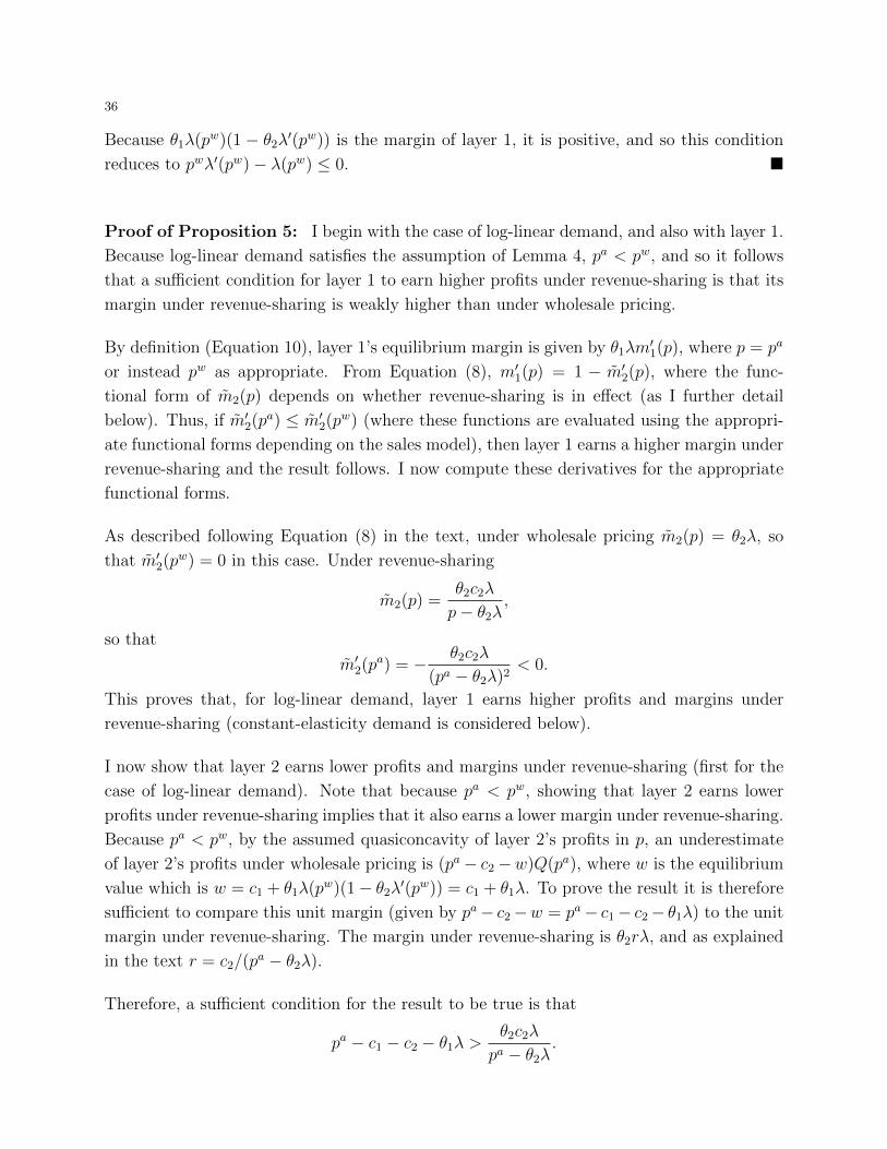
36

Because θ1λ(pw)(1 − θ2λ′(pw)) is the margin of layer 1, it is positive, and so this condition

reduces to pwλ′(pw)− λ(pw) ≤ 0. �

Proof of Proposition 5: I begin with the case of log-linear demand, and also with layer 1.

Because log-linear demand satisfies the assumption of Lemma 4, pa < pw, and so it follows

that a sufficient condition for layer 1 to earn higher profits under revenue-sharing is that its

margin under revenue-sharing is weakly higher than under wholesale pricing.

By definition (Equation 10), layer 1’s equilibrium margin is given by θ1λm′1(p), where p = pa

or instead pw as appropriate. From Equation (8), m′1(p) = 1 − m′2(p), where the func-

tional form of m2(p) depends on whether revenue-sharing is in effect (as I further detail

below). Thus, if m′2(pa) ≤ m′2(pw) (where these functions are evaluated using the appropri-

ate functional forms depending on the sales model), then layer 1 earns a higher margin under

revenue-sharing and the result follows. I now compute these derivatives for the appropriate

functional forms.

As described following Equation (8) in the text, under wholesale pricing m2(p) = θ2λ, so

that m′2(pw) = 0 in this case. Under revenue-sharing

m2(p) =θ2c2λ

p− θ2λ,

so that

m′2(pa) = − θ2c2λ

(pa − θ2λ)2< 0.

This proves that, for log-linear demand, layer 1 earns higher profits and margins under

revenue-sharing (constant-elasticity demand is considered below).

I now show that layer 2 earns lower profits and margins under revenue-sharing (first for the

case of log-linear demand). Note that because pa < pw, showing that layer 2 earns lower

profits under revenue-sharing implies that it also earns a lower margin under revenue-sharing.

Because pa < pw, by the assumed quasiconcavity of layer 2’s profits in p, an underestimate

of layer 2’s profits under wholesale pricing is (pa− c2−w)Q(pa), where w is the equilibrium

value which is w = c1 + θ1λ(pw)(1− θ2λ′(pw)) = c1 + θ1λ. To prove the result it is therefore

sufficient to compare this unit margin (given by pa− c2−w = pa− c1− c2− θ1λ) to the unit

margin under revenue-sharing. The margin under revenue-sharing is θ2rλ, and as explained

in the text r = c2/(pa − θ2λ).

Therefore, a sufficient condition for the result to be true is that

pa − c1 − c2 − θ1λ >θ2c2λ

pa − θ2λ.

37

Using Equation (12) to rewrite the left-hand side, and then dividing through by θ2c2λ and

multiplying through by (pa − θ2λ)2, this condition reduces to

pa + λ(θ1 − θ2) > pa − θ2λ⇐⇒ θ1λ > 0

which is true.

I now consider the constant-elasticity case (Q(p) = p−1/σ, λ(p) = σp, for σ ∈ (0, 1)). Direct

computation using Equations (11) and (12) gives

pa =c1 + c2 − c1σθ2

(1− σθ1)(1− σθ2), and pw =

c1 + c2

(1− σθ1)(1− σθ2).

Consider the second-mover. Its profits under wholesale pricing are

θ2λ(pw)Q(pw) = θ2σ(pw)(σ−1)/σ,

given that Q(p) = p−1/σ. Under revenue-sharing, its profits are

rθ2λ(pa)Q(pa) =c2θ2λ(pa)

pa − θ2λ(pa)Q(pa) =

c2θ2σ

1− θ2σQ(pa) =

c2θ2σ

1− θ2σ(pa)−1/σ.

Using the values for pa and pw explicitly given above, the ratio of profits under wholesale

pricing to revenue-sharing isc1 + c2(1− σθ1)

c2(1− σθ1)> 1.

This proves the result for the second-mover. Now consider the first-mover, whose profits

under revenue-sharing are

[(1− r)pa − c1]Q(pa) =

[pa − c2p

a

pa − θ2λ(pa)− c1

]Q(pa) =

[pa − c2

1− σθ2

− c1

](pa)−1/σ.

Under wholesale pricing, its profits are

θ1λ(pw)(1− θ2λ′(pw))Q(pw) = θ1σ(1− θ2σ)(pw)(σ−1)/σ.

Using the values for pw and pa given above, taking the ratio of profits under revenue-sharing

to those under wholesale pricing gives(1

1− σθ2

)(c1 + c2

c1 + c2 − c1σθ2

) 1−σσ

> 1,

where the inequality follows because each of the two terms that are multiplied together on

the left-hand side is greater than one. This completes the proof. �

Proof of Proposition 6: Note that this proof uses facts in the text given following Equa-

tion (8) and that all demand functions considered here satisfy the properties of Lemma 4,

so that pa < pw.

38

I begin with D for the case of (weakly) log-concave demand. Because pa < pw more units are

sold under the agency model and so to show that a switch from the wholesale model to the

agency model benefits (layer) D it is enough to show that D’s per-unit margin is higher under

the agency model. D’s margin under the wholesale model is θDλ(pw) ≤ θDλ(pa), where the

inequality follows from the fact that demand is log-concave (so that λ(p) is non-increasing)

and pa < pw . Under the agency model, from Equation (10) the margin of D is

θDλ(pa)m′1(pa) = θDλ(pa)[1− m′2(pa)] = θDλ(pa)

[1− θUcU

(paλ′(pa)− λ(pa))

(pa − θUλ(pa))2

]. (22)

Because paλ′(pa)− λ(pa) < 0 for weakly log-concave demand, this margin exceeds θDλ(pa),

which as explained above is an upper bound on the margin of D under the wholesale model.

Because D sells more units under the agency model, the result follows.

Now consider D when demand is constant-elasticity (Q(p) = p−1/σ, λ(p) = σp, for σ ∈ (0, 1)).

Here it is necessary to directly compute the profits of D. Under the agency model, Equation

(22) above applies to D’s margin, but specializing to the case of constant-elasticity demand

gives D’s margin as θDλ(pa) = θDσpa, and hence total profits of θDσp

aQ(pa). Under the

wholesale model, D’s margin is θDλ(pw) = θDσpw, for total profits of θDσp

wQ(pw).

Direct computation using Equations (11) and (12) gives, for constant-elasticity demand,

pa =cD + cU − cDσθU

(1− σθD)(1− σθU), and pw =

cD + cU(1− σθD)(1− σθU)

.

From this it can be shown that profits are higher under the agency model so long as

cD(1− σθU) + cU < cD + cU ,

which is true.

I now show that U is worse off under the agency model. Because pa < pw, and because layer

1’s profits are assumed to be quasiconcave in p, under the wholesale model an underestimate

of layer U ’s profit is the profit that layer 1 would get if it set p = pa:

m1(pa)Q(pa) = [pa − cD − cU − m2(pa)]Q(pa) = [pa − cD − cU − θDλ(pa)]Q(pa)

= θUcUλ(pa)

[pa(1− θDλ′(pa)) + λ(pa)(θD − θU)

(pa − θUλ(pa))2

]Q(pa),

where the final equality follows from Equation (12), and keeping in mind that that equation

is for the price under the agency model in which U is firm 2. Now consider U ’s profits under

the agency model:

rθUλ(pa)Q(pa) =θUcUλ(pa)

pa − θUλ(pa)Q(pa),

39

so that a sufficient condition for wholesale profits to be higher is that

pa(1− θDλ′(pa)) + λ(pa)(θD − θU)

(pa − θUλ(pa))2≥ 1

pa − θUλ(pa)⇐⇒ θD(paλ′(pa)− λ(pa)) ≤ 0.

This condition is satisfied for all the demand functions considered in this proposition. Hence

U is worse off under the agency model. �

Proof of Proposition 7: I begin by confirming that Equation (14) indeed characterizes

the symmetric equilibrium for any given industry-wide value of w, with or without MFNs.

Without MFNs, the first-order conditions for p and p (from Equation (13)) are

Q(p, p, p, p) + (p− w − cU)Q1(p, p, p, p) + (p− w − cU)Q2(p, p, p, p) = 0, (23)

and

Q(p, p, p, p) + (p− w − cU)Q1(p, p, p, p) + (p− w − cU)Q2(p, p, p, p) = 0. (24)

At a symmetric industry solution with all retailers setting the same wholesale price w and

all suppliers are setting the same price p through all retailers, the margin of a supplier is

p− w − cU = − Q(p)

Q1(p) +Q2(p),

as claimed in the text.

Suppose now that price-parity restrictions are in place, and once again consider a given

supplier facing wholesale prices of w and w. Because this supplier is constrained to set its

retail prices so that p = p, its profits are

(p− w − cU)Q(p, p, p, p) + (p− w − cU)Q(p, p, p, p),

with a single corresponding first-order condition

2Q(p, p, p, p) + [(p− w − cU) + (p− w − cU)] [Q1(p, p, p, p) +Q2(p, p, p, p)] = 0. (25)

At a symmetric industry outcome in retail and wholesale prices, this gives

p− w − cU = − Q(p)

Q1(p) +Q2(p).

This is identical to Equation (14). Thus, facing a given industry-wide wholesale price w,

suppliers set the same markups whether retail price-parity restrictions are in effect or not.

To show that industry-wide price parity raises industry prices, I compare Equations (16) and

(17). These margins are positive, and so the denominators in both expressions are negative.

Hence, given that the right-hand side of these equations is decreasing in the industry-wide

wholesale price w being charged, the downstream margin is larger under retail price-parity

40

restrictions if

Q1(p)pM1 +Q2(p)pM1 > Q1(p)p1 +Q2(p)p1.

Because Q1 < 0 < Q2 and because pM1 > 0,41 a sufficient condition for this is that p1 > pM1 >

p1. I will show that this condition holds, so that indeed price-parity raises the industry-

wide equilibrium wholesale price w. Because p∗(w) is increasing, it will also follow that the

industry retail price is higher under price parity.

I will show that pM1 = (p1 + p1)/2 and also that p1 > p1, which implies the desired con-

dition. To this end, let Π(p, p) denote the profits of an upstream firm, which are given in

Equation (13). Absent price parity, the first-order conditions are Πp = 0 and Πp = 0, using

subscripts to denote the variable of differentiation. A small change in w must maintain these

first-order conditions, so that the following equations hold:

Πpw + Πppp1 + Πppp1 = 0, and Πpw + Πppp1 + Πppp1 = 0.

Solving for p1 and p1 at a symmetric solution, and using the fact that the symmetry of the

problem implies that Πpp = Πpp, gives

p1 =−ΠpwΠpp + ΠpwΠpp

Π2pp − Π2

pp

, and p1 =−ΠpwΠpp + ΠpwΠpp

Π2pp − Π2

pp

.

To find pM1 , note that profits in the case with retail price-parity are also given by Π(p, p), but

of course subject to the constraint that p = p. The relevant first-order condition emerges

from the fact that an increase in p must be accompanied by an equal increase in p, so that

Πp + Πp = 0. To maintain this condition following an increase in w requires that

Πpw + ΠpppM1 + Πppp

M1 + Πpw + Πppp

M1 + Πppp

M1 = 0.

This gives

pM1 =−Πpw − Πpw

2(Πpp + Πpp).

Direct computation gives

p1 + p1

2=

1

2

[(−Πpw − Πpw)(Πpp − Πpp)

Π2pp − Π2

pp

]=

1

2

[−Πpw − Πpw

Πpp + Πpp

]= pM1 .

Thus, to complete the proof it is enough to show that p1 > p1. Using the expressions above

for these functions, and using the standard sufficient condition for optimality Π2pp−Π2

pp > 0

41pM is increasing in w under the maintained regularity conditions that the optimal decisions of firms are uniquelycharacterized by their first-order conditions. For the present situation, this means that (manipulating Equation (25)),a supplier’s first-order condition under MFNs is

p− (w + w)

2− cU = − Q(p, p, p, p)

Q1(p, p, p, p) +Q2(p, p, p, p).

The right-hand side is assumed to intersect the left-hand side from above. Thus an increase in w raises p.

41

(taking advantage of the symmetry of the problem, so that Πpp = Πpp), p1 > p1 if

(Πpp + Πpp)(Πpw − Πpw) = (Πpp + Πpp)(−Q2(p) +Q1(p)) > 0,

where the equality follows from directly computing Πpw and Πpw from Equation (13). Be-

cause Q1(p) < 0 < Q2(p), it follows that −Q2(p) + Q1(p) < 0, so that the inequality holds

if Πpp + Πpp < 0. But this condition is equivalent to the marginal profitability of raising

both p and p being decreasing, which is simply part of the overall sufficient condition for

optimality.42 Hence, Πpp − Πpp < 0, and the conclusion follows. �

Proof of Proposition 8: First I show that the margin that suppliers set under revenue-

sharing is not affected by whether price-parity restrictions are in place, for a given set of

symmetric contracts. Under the case of wholesale pricing, consider, say, supplier 1’s pricing

decision. This supplier’s profits are

(p1 − w − cU)Q(p1, p1, p2, p2) + (p1 − w − cU)Q(p1, p1, p2, p2). (26)

Obtaining the first-order conditions and looking at a symmetric industry equilibrium (w =

w, p = p1 = p2 = p1 = p2), this leads to the analogue of Equation (14),

p− w − cU = − Q(p)

Q1(p) +Q2(p).

Moreover, as before, this is the correct margin whether or not price-parity holds, following

the same steps as for Proposition 7 (imposing p1 = p1). When wholesale prices are in effect,

let p∗(w) denote the price satisfying the above equation, so that p∗(w) gives the price that

would be set by both suppliers given that both suppliers face the wholesale price w, where

p∗(w) is increasing.

Under revenue-sharing, the only difference compared to wholesale pricing is that the per-unit

margins in Equation (26) are replaced by rp1− cU and rp1− cU , where r is the revenue share

offered by retailer A and r is the revenue-share offered by retailer B. But then taking the

same steps as before (that is, differentiating with respect to p1 and p1) leads to the conclusion

that, at a symmetric outcome in which both retailers set the same contract (r = r) and all

retail prices equal p, and with or without price-parity restrictions, the margin of suppliers is

rp− cU = −r Q(p)

Q1(p) +Q2(p). (27)

For arbitrary r, and in an abuse of notation, let p∗(r) denote the solution to Equation (27).

This gives the price that suppliers would charge if they both faced the same revenue-share

42The marginal profits of raising both p and p must be zero: Πp+Πp = 0. Also, these marginal profits must decreasewhen both p and p are further raised: Πpp + Πpp + Πpp + Πpp < 0. The symmetry of the problem means Πpp = Πpp,giving the condition Πpp + Πpp < 0.

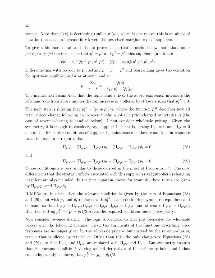
42

term r. Note that p∗(r) is decreasing (unlike p∗(w), which is one reason this is an abuse of

notation) because an increase in r lowers the perceived marginal cost of suppliers.

To give a bit more detail and also to prove a fact that is useful below, note that under

price-parity (where it must be that p1 = p1 and p2 = p2) this supplier’s profits are

(rp1 − cU)Q(p1, p1, p2, p2) + (rp1 − cU)Q(p1, p1, p2, p2).

Differentiating with respect to p1, setting p = p1 = p2 and rearranging gives the condition

for upstream equilibrium for arbitrary r and r:

p− 2cUr + r

= − Q(p)

Q1(p) +Q2(p).

The maintained assumption that the right-hand side of the above expression intersects the

left-hand side from above implies that an increase in r offered by A lowers p, so that pM1 < 0.

The next step is showing that pM1 = (p1 + p1)/2, where the function pM1 describes how all

retail prices change following an increase in the wholesale price charged by retailer A (the

case of revenue-sharing is handled below). I first consider wholesale pricing. Given the

symmetry, it is enough to consider, say, supplier 1. That is, letting Πp1 = 0 and Πp1 = 0

denote the first-order conditions of supplier 1, maintenance of these conditions in response

to an increase in w requires that

Πp1w + (Πp1p1 + Πp1p2) p1 + (Πp1p1 + Πp1p2) p1 = 0, (28)

and

Πp1w + (Πp1p1 + Πp1p2) p1 + (Πp1p1 + Πp1p2) p1 = 0. (29)

These conditions are very similar to those derived in the proof of Proposition 7. The only

difference is that the strategic effects associated with this supplier’s rival (supplier 2) changing

its prices are also included. In the first equation above, for example, these terms are given

by Πp1p2p1 and Πp1p2 p1.

If MFNs are in place, then the relevant condition is given by the sum of Equations (28)

and (29), but with p1 and p1 replaced with pM1 . I am considering symmetric equilibria and

demand, so that Πp1p1 = Πp1p1 ,Πp1p2 = Πp1p2 ,Πp1p2 = Πp1p2 (and of course Πp1p1 = Πp1p1).

But then setting pM1 = (p1 + p1)/2 solves the required condition under price-parity.

Now consider revenue-sharing. The logic is identical to that just presented for wholesale

prices, with the following changes. First, the arguments of the functions describing price

responses are no longer given by the wholesale price w but instead by the revenue-sharing

term r that is offered by retailer A. Other than this, the only changes to Equations (28)

and (29) are that Πp1w and Πp1w are replaced with Πp1r and Πp1r. But symmetry ensures

that the various equalities involving second derivatives of Π continue to hold, and I thus

conclude, exactly as above, that pM1 = (p1 + p1)/2.

43

To show that this implies that competition between retailers in terms of trade is softened,

and that retail prices are therefore increased by price-parity clauses, only a few steps remain.

The first of these is the derivation of the downstream margin. The same steps are followed

as before. For example, with wholesale pricing, retailer A’s profits are

(w − cD)[Q(p1, p1, p2, p2) +Q(p2, p2, p1, p1)

].

The reason is that supplier 1 sells Q(p1, p1, p2, p2) units through A, while supplier 2 sells

Q(p2, p2, p1, p1) through A. Let p denote the common price set by suppliers at A and let

p denote the common price set by suppliers at B (that is, p = p1 = p2 and p = p1 = p2).

Profits are proportional to (w− cD)Q(p, p, p, p). Suppressing arguments for compactness and

considering the effect of A raising the wholesale price w it charges both suppliers yields the

first-order condition

Q+ (w − cD) [(Q1 +Q3)p1 + (Q2 +Q4)p1] = 0,

This differs from before to the extent that it accommodates how the prices of all goods

(through any retailer) change following the increase in w. Evaluating at a symmetric industry

solution, and letting for example Q3(p) denote the change in Q(p, p, p, p) from a small change

in the third argument, the margin of retailers is given by

w − cD = − Q(p∗(w))

[Q1(p∗(w)) +Q3(p∗(w))] p1(w,w) + [Q2(p∗(w)) +Q4(p∗(w))] p1(w,w). (30)

Note that I have written Equation (30) to be explicit about the arguments of all functions

so that it is clear exactly what the equilibrium condition involving the retailers is. In line

with earlier assumptions, the right-hand side of the above expression intersects the left-hand

side from above as the industry-wide wholesale price w changes. Hence the question will be

how the relevant expression changes when price-parity is in effect. When it is in effect, the

only change is that p1 and p1 are replaced with pM1 . Thus, if the right-hand side is larger

under price-parity, the equilibrium wholesale price is higher, meaning that (because p∗(w) is

increasing) the equilibrium retail price is higher. Because the denominator in the right-hand

side is negative (ensuring a non-negative margin for retailers), the right-hand side is larger

under price-parity if

(Q1 +Q3)p1 + (Q2 +Q4)p1 < (Q1 +Q3)pM1 + (Q2 +Q4)pM1 .

Because Q1 and Q3 are negative (because they measure the effect on retailer A’s sales when

both suppliers raise the price they set through retailer A), and because Q2 and Q4 are

positive (because they measure the effect on retailer A’s sales when both suppliers raise the

price they set through retailer B), a sufficient condition is that (i) p1 > pM1 > p1, and (ii)

44

pM1 > 0. As before, however, pM1 > 0, and so it is sufficient that p1 > p1.43 This is true by

assumption, and so the equilibrium wholesale price is indeed higher under price-parity.

Now I consider the effect of price-parity under revenue-sharing, in particular considering the

effect on retailers. Consider the profits of retailer A, given by

[(1− r)p− cD][Q(p1, p1, p2, p2) +Q(p2, p2, p1, p1)].

At an outcome where both suppliers charge p through retailer A and p through retailer B,

these profits are proportional to [(1 − r)p − cD]Q(p, p, p, p). Consider this retailer choosing

r, where I will write the first-order condition suppressing the arguments of Q for notational

compactness. Because I am interested in a symmetric outcome (r = r and all prices given

by p), the first-order condition at equilibrium can be written as

[−p+ (1− r)p1]Q+ [(1− r)p− cD] [(Q1 +Q3)p1 + (Q2 +Q4)p1] = 0.

Thus, at a symmetric industry solution where both retailers set revenue shares equal to r,

the margin (1 − r)p − cD of this retailer satisfies the following, where to be as explicit as

possible I write all of the arguments of the functions out fully.

(1− r)p∗(r)− cD =[p∗(r)− (1− r)p1(r, r)]Q(p∗(r))

[Q1(p∗(r)) +Q3(p∗(r))] p1(r, r) + [Q2(p∗(r)) +Q4(p∗(r))] p1(r, r). (31)

Under price-parity, the same expression emerges but with pM1 taking the place of p1 and

p1. For the equilibrium retail price to be higher under price-parity, it is enough that the

equilibrium revenue-sharing term r is smaller under price-parity. The analogue of earlier

assumptions is that the right-hand side of Equation (31) intersects the left-hand side once

and from above as 1 − r increases (or equivalently, as p increases, letting the industry-

level r equilibrate according to the function p∗(r)). Hence, and now suppressing unneeded

notational elements for simplicity, price-parity lowers the industry revenue-share term r if

p− (1− r)pM1(Q1 +Q3)pM1 + (Q2 +Q4)pM1

>p− (1− r)p1

(Q1 +Q3)p1 + (Q2 +Q4)p1

. (32)

Earlier in this proof I showed that (under revenue-sharing) pM1 < 0 and also that pM1 =

(p1 + p1)/2. Furthermore, by the conditions of the proposition, p1 < p1. Thus, it follows

that p1 < pM1 < p1 and also p1 < pM1 < 0. Because Q1 + Q3 < −(Q2 + Q4) < 0, these

observations imply that the denominators are positive. In turn, because the overall margins

must be positive, the numerators must be positive.

43To be precise, pM1 > 0 so long as the condition

p− (w + w)

2− cU = − Q(p)

Q1(p) +Q2(p)

is such that the right-hand side intersects the left-hand side from above. This just says industry profits are quasi-concave in the industry price p.

45

To prove that the inequality in (32) holds, I will first argue that

p

(Q1 +Q3)pM1 + (Q2 +Q4)pM1>

p

(Q1 +Q3)p1 + (Q2 +Q4)p1

.

This holds so long as

(Q1 +Q3)p1 + (Q2 +Q4)p1 > (Q1 +Q3)pM1 + (Q2 +Q4)pM1 .

Because (Q1 + Q3) < 0, and because p1 < pM1 < 0, it is sufficient that (Q2 + Q4)p1 >

(Q2 +Q4)pM1 . Because (Q2 +Q4) > 0, in turn it is sufficient that p1 > pM1 , which I already

showed. Hence, to prove that Equation (32) holds, it is enough to show that (after eliminating

the common term −(1− r) < 0)

pM1(Q1 +Q3)pM1 + (Q2 +Q4)pM1

<p1

(Q1 +Q3)p1 + (Q2 +Q4)p1

.

Multiplying through and simplifying, and again using the facts that (i) the denominators

are positive, (ii) Q2 + Q4 > 0, and (iii) pM1 < 0, this reduces to the condition that p1 < p1,

which is true by the conditions of the proposition. �

References

Adachi, T. and T. Ebina (2014). Double marginalization and cost pass-through: Weyl-

fabinger and cowan meet spengler and bresnahan-reiss. Economics Letters 122 (2), 170–

175.

Amir, R., I. Maret, and M. Troege (2004). On taxation pass-through for a monopoly firm.

Annales d’conomie et de Statistique (75/76), 155–172.

Anderson, S. P., A. De Palma, and B. Kreider (2001). The efficiency of indirect taxes under

imperfect competition. Journal of Public Economics 81 (2), 231–251.

Bagnoli, M. and T. Bergstrom (2005). Log-concave probability and its applications. Eco-

nomic Theory 26 (2), 445–469.

Baker, J. B. (1996). Vertical restraints with horizontal consequences: Competitive effects of

“most-favored-customer” clauses. Antitrust Law Journal 64, 517–34.

Bishop, R. L. (1968). The effects of specific and ad valorem taxes. Quarterly Journal of

Economics 82 (2), 198–218.

Boik, A. and K. S. Corts (2016). The effects of platform most-favored-nation clauses on

competition and entry. Journal of Law and Economics 59 (1), 105–134.

Bonanno, G. and J. Vickers (1988). Vertical separation. Journal of Industrial Econom-

ics 36 (3), 257–265.

Cachon, G. P. and M. A. Lariviere (2005). Supply chain coordination with revenue-sharing

contracts: Strengths and limitations. Management Science 51 (1), 30–44.

46

Dana, J. D. and K. E. Spier (2001). Revenue sharing and vertical control in the video rental

industry. Journal of Industrial Economics 49 (3), 223–245.

DeGraba, P. and A. Postlewaite (1992). Exclusivity clauses and best price policies in input

markets. Journal of Economics and Management Strategy 1 (3), 421–454.

Edelman, B. G. and J. Wright (2015). Price coherence and excessive intermediation. Quar-

terly Journal of Economics 130, 1283–1328.

Foros, Ø., H. J. Kind, and G. Shaffer (2015). Apple’s agency model and the role of resale

price maintenance. Working Paper .

Gans, J. (2012). Mobile application pricing. Information Economics and Policy 24, 52–59.

Gaudin, G. and A. White (2014a). On the antitrust economics of the electronic books

industry. Working Paper .

Gaudin, G. and A. White (2014b). Unit vs. ad valorem taxes under revenue maximization.

Working Paper .

Hagiu, A. and J. Wright (2015). Marketplace or reseller? Management Science 61 (1),

184–203.

Johansen, B. O. and T. Verge (2016, September). Platform price parity clauses with direct

sales. Working Paper .

Johnson, J. P. (2013). The agency and wholesale models in electronic content markets.

Working Paper .

Kourandi, F. and N. Vettas (2012). Endogenous spatial differentiation with vertical con-

tracting. Working Paper .

Krishnan, H., R. Kapuscinski, and D. A. Butz (2004). Coordinating contracts for decentral-

ized supply chains with retailer promotional effort. Management Science 50 (1), 48–63.

Lin, Y. J. (1990). The dampening-of-competition effect of exclusive dealing. Journal of

Industrial Economics 39 (2), 209–223.

Llobet, G. and J. Padilla (2014). The optimal scope of the royalty base in patent licensing.

Working Paper .

Loertscher, S. and A. Niedermayer (2015, August). Percentage fees in thin markets: An

optimal pricing perspective. Working Paper .

Mathewson, G. F. and R. A. Winter (1985). The economics of franchise contracts. Journal

of Law and Economics 28 (3), 503–526.

McAfee, R. P. and M. Schwartz (1994). Opportunism in multilateral vertical contracting:

Nondiscrimination, exclusivity, and uniformity. American Economic Review 84 (1), 210–

230.

Reisinger, M. and M. Schnitzer (2012). Successive oligopolies with differentiated firms and

endogeneous entry. Journal of Industrial Economics 60 (4), 537–577.

Rey, P. and J. Stiglitz (1995). The role of exclusive territories in producers’ competition.

RAND Journal of Economics 26 (3), 431–451.

47

Salinger, M. A. (1988). Vertical mergers and market foreclosure. Quarterly Journal of

Economics 103 (2), 345–356.

Skeath, S. E. and G. A. Trandel (1994). A pareto comparison of ad valorem and unit taxes.

Journal of Public Economics 53, 53–71.

Suits, D. B. and R. A. Musgrave (1953). Ad valorem and unit taxes compared. Quarterly

Journal of Economics 67 (4), 598–604.

Wang, Z. and J. Wright (2017, forthcoming). Ad-valorem platform fees, indirect taxes and

efficient price discrimination. RAND Journal of Economics .

Weyl, E. G. and M. Fabinger (2013). Pass-through as an economic tool: principles of

incidence under imperfect competition. Journal of Political Economy 121 (3), 528–583.