The Agency Model and MFN Clauses

Justin P. Johnson†

May 1, 2015

Abstract. I provide a general analysis of vertical relations that are intermediated

either with wholesale prices or with revenue-sharing contracts. Although revenue-

sharing does not eliminate double markups, it nonetheless tends to lower retail

prices. Revenue-sharing is extremely attractive to the firm that is able to set the

revenue shares, but often makes the other firm worse off. These results hold even

when there is imperfect competition at both layers of the supply chain. I also

show that retail price-parity restrictions raise industry prices. These results explain

why many online retailers have adopted the “agency model” (in which they set

revenue shares and suppliers set retail prices) and price-parity clauses. Finally, in

an extension that considers private bargaining, I show that unobservable delegations

can have equilibrium effects, and identify how pricing discretion can improve a firm’s

bargaining position.

It is common for vertical relations to be structured so that one firm sets the “terms of trade”

governing exchange with another firm that then sets a retail price to end consumers. These

terms of trade stipulate either a per-unit commission or instead a revenue-sharing term. In

this article I present a general analysis of such vertical relations. I also investigate the effect

of retail price-parity restrictions such as most-favored nation clauses.

My analysis encompasses not only bilateral monopoly but also bilateral imperfect competi-

tion (in which there is market power at both stages of supply), and allows for flexibility in

which firms in the supply chain set the terms of trade and which set retail prices. Thus, for

example, not only am I able to compare how revenue-sharing differs from constant commis-

sions given that the same firms set the terms of trade in either circumstance, but I am also

able to assess the effects of a change in which firms set these terms.

This flexibility allows me to evaluate an important shift that is taking place in retailing,

especially in online markets. Traditionally, it has been most common for suppliers to set

wholesale prices and retailers to set retail prices; this is called the “wholesale model of sales.”

With growing prevalence, however, online retailers instead specify a share of revenue that

their suppliers will receive, with suppliers then setting the retail price; this is called the

“agency model of sales.”

I thank Rabah Amir, Aaron Edlin, Justin Ho, Thomas Jeitschko, Jin Li, Sridhar Moorthy, Daniel O’Brien, TonyCurzon Price, Thomas Ross, Henry Schneider, and Michael Waldman. I especially thank Marco Ottaviani, YossiSpiegel, Glen Weyl, and three anonymous referees for extensive comments.†Johnson Graduate School of Management, Cornell University. Email: jpj25@cornell.edu.

2

For example, the online retailer Amazon uses the agency model in operation of its exchange

for a vast variety of retail goods called the “Amazon Marketplace,” which accounts for over

40% of the products it sells globally.1 Amazon’s leading online competitor, eBay, also uses

the agency model when merchants sell goods using the fixed-price rather than the auction

format (eBay now emphasizes the fixed-price format over the auction format, and it accounts

for more than half of all of eBay’s sales). Products as diverse as e-books, applications for

mobile devices such as smartphones and tablets, car insurance, and hotel reservations have

been sold online using the agency model.

In many of the markets just mentioned, retail most-favored nation contracts (MFNs) have

been used. In essence, these terms insist that a supplier cannot set a lower price through

one online retailer than through another. The use of MFNs has led to regulatory scrutiny,

for example of the Amazon Marketplace, price-comparison websites reselling private motor

insurance, the e-book market, and online travel agencies such as Expedia and Booking.com.

Before describing my results, I note that revenue-sharing does not eliminate the double-

marginalization problem; double markups remain, but are more subtle. In particular, when

the firm setting the revenue share keeps some revenue for itself, the firm setting the retail

price bears the entirety of its own costs but receives only a portion of revenue, causing it to

act as if its costs are higher than they actually are; this is one markup. The second markup

is that which the firm setting retail prices imposes over these perceived marginal costs.

My main results are as follows. First, regardless of the shape of demand, when revenue-

sharing is used each firm prefers to be the one that sets revenue shares rather than being the

one that sets retail prices. This result is non-obvious because under the commission model,

whether it is better to set the terms of trade (given by a wholesale price) or instead the retail

price depends on the log-curvature of demand.

Second, despite the fact that double markups do exist under revenue-sharing, the equilibrium

retail price tends to be lower. This is true even when there is imperfect competition at both

layers of the supply chain. However, in the presence of such competition, the lower prices

under revenue-sharing may well lower industry profits.

Even though revenue-sharing may therefore lower industry profits, my third main result is

that, given that a firm would set the terms of trade regardless of whether revenue-sharing

or instead constant commissions are used, it prefers revenue-sharing under a broad set of

circumstances. Indeed, it may even earn higher per-unit margins under revenue-sharing,

rather than simply earning higher profit. To be perfectly clear, this profitability result is

true even when there is imperfect competition at both layers of the supply chain.

1See “OFT minded to drop investigation into Amazon pricing policies,” Financial Times, August 29, 2013.

3

Fourth, the firms that set retail prices are often worse off under revenue-sharing. This is

true even if the lower prices associated with revenue-sharing raise industry profits (as is the

case under bilateral monopoly). Thus, revenue-sharing can be seen as a weapon that one

firm uses to its own advantage but to the detriment of other firms.

When a move to revenue-sharing is accompanied by a switch in which firm sets the retail

price, as when there is a move from the wholesale model to the agency model, these results

continue to hold (and may be strengthened): a shift from the wholesale model to the agency

model tends to make the retailer better off but the supplier worse off.

These results explain why retailers such as Amazon, Apple, and eBay might benefit from

competing using the agency model rather than the wholesale model, and why they would

wish to set the revenue-sharing terms themselves rather than have suppliers do it.

In essence, the intuition for all of these results is as follows. Suppose that the firm setting

retail prices pays the other firm a constant commission per unit sold. When this firm raises

the retail price by one, its own per-unit margin therefore increases by one. In contrast, when

revenue-sharing is in effect, an increase of one in the retail price is only partially captured

by the firm setting that price. That is, its own per-unit margin increases by less than one,

because it must share the extra revenue from the price increase with the other firm. This

effect diminishes the effectiveness of price increases under revenue-sharing. Thus, compared

to the commission-based model of sales, revenue-sharing puts the firm setting retail prices

in a difficult position, a fact that the firm setting the revenue-share is able to exploit to its

own benefit and the other firm’s harm.

Another main result is that price-parity restrictions in the form of retail MFN contracts tend

to raise industry prices. In particular, MFNs kill a retailer’s incentives to compete in the

terms of trade that it offers suppliers. The reason is that a retailer who raises the commission

it charges (or offers suppliers a lower revenue share) knows that the price set through its

store will not increase relative to that at other stores. Indeed, the essence of price parity

is that affected suppliers must raise the price that they set through all stores if they are to

raise prices at all. This effect encourages retailers to charge higher fees to suppliers, which

in equilibrium raises the final retail price and harms consumers.

The prospect that MFNs might lead to higher retail prices—and negate any positive effects

from a switch to the agency model—suggests that such contracts ought to be carefully

scrutinized. Indeed, concerns have been expressed in multiple antitrust investigations in

the US and the EU, as I discuss in more detail later. However, I also discuss potential

pro-competitive effects of price-parity clauses.

4

My final contribution is to consider a private bargaining environment in which the identity

of the firms that set retail prices is determined contractually, and in which contracts include

fixed fees. This extends the analysis of O’Brien and Shaffer (1992).

In this setting, two main results emerge. First, even though contracting is private, equi-

librium prices and hence industry profits depend on which firms have the discretion to set

retail prices. This is interesting because it has been argued that the delegation of decision

rights can have no effect on equilibrium outcomes when negotiations are private (see Katz

(1991)). Thus, I identify a new rationale for why strategic delegation can have equilibrium

effects.2 Second, the equilibrium allocation of pricing discretion affects the distribution of

industry profits. In particular, the layer of the supply chain that sets prices receives a higher

share of industry profits than the other layer, regardless of the curvature of demand. The

reason is that the firm with pricing discretion is able to better respond to out-of-equilibrium

contracts, which strengthens its bargaining position. This suggests there may be a tension

in the allocation of pricing discretion: an individual firm may prefer such discretion even if

it leads to lower industry profits (and even when fixed fees are used).

I now briefly discuss some of the related literature; other contributions are discussed as the

opportunity arises. The effect of revenue-sharing alone has been investigated both in the

economics and operations research literatures (for example, Mathewson and Winter (1985),

Dana and Spier (2001), Cachon and Lariviere (2005), and Krishnan, Kapuscinski, and Butz

(2004)). Although very interesting, these articles are quite different in focus and consider

neither supplier retail-price setting nor market power at both the manufacturing and re-

tailing stages. There are several related contributions to the economics of platforms. Gans

(2012) argues that most-favored nation contracts can resolve a holdup problem. Boik and

Corts (2013) argue as I do that MFNs may work to raise final retail prices, but do not con-

sider differences between the agency model and wholesale models or accommodate imperfect

competition both at the supplier and retailer levels. Hagiu and Wright (2013) consider the

choice between what they call a “marketplace” (the agency model in my terminology) and a

“reseller” (the wholesale model in my terminology). They emphasize the importance of non-

contractible decisions of suppliers in the determination of optimal supply chain structure.

My paper is organized as follows. Section 1 analyzes bilateral monopoly, which is extended in

Section 2 to bilateral imperfect competition. Section 3 assesses price-parity clauses. Section

4 considers the environment with private contracting and general contracts.

2Related work on the delegation effects of vertical structure includes, for example, Bonanno and Vickers (1988), Lin(1990), and Rey and Stiglitz (1995). They argue, respectively, that vertical separation, exclusivity provisions, andexclusive territory restrictions may raise retail prices by softening supplier competition. Note that the results that Idiscussed earlier hold in a model of bilateral monopoly in which such softening effects are necessarily absent.

5

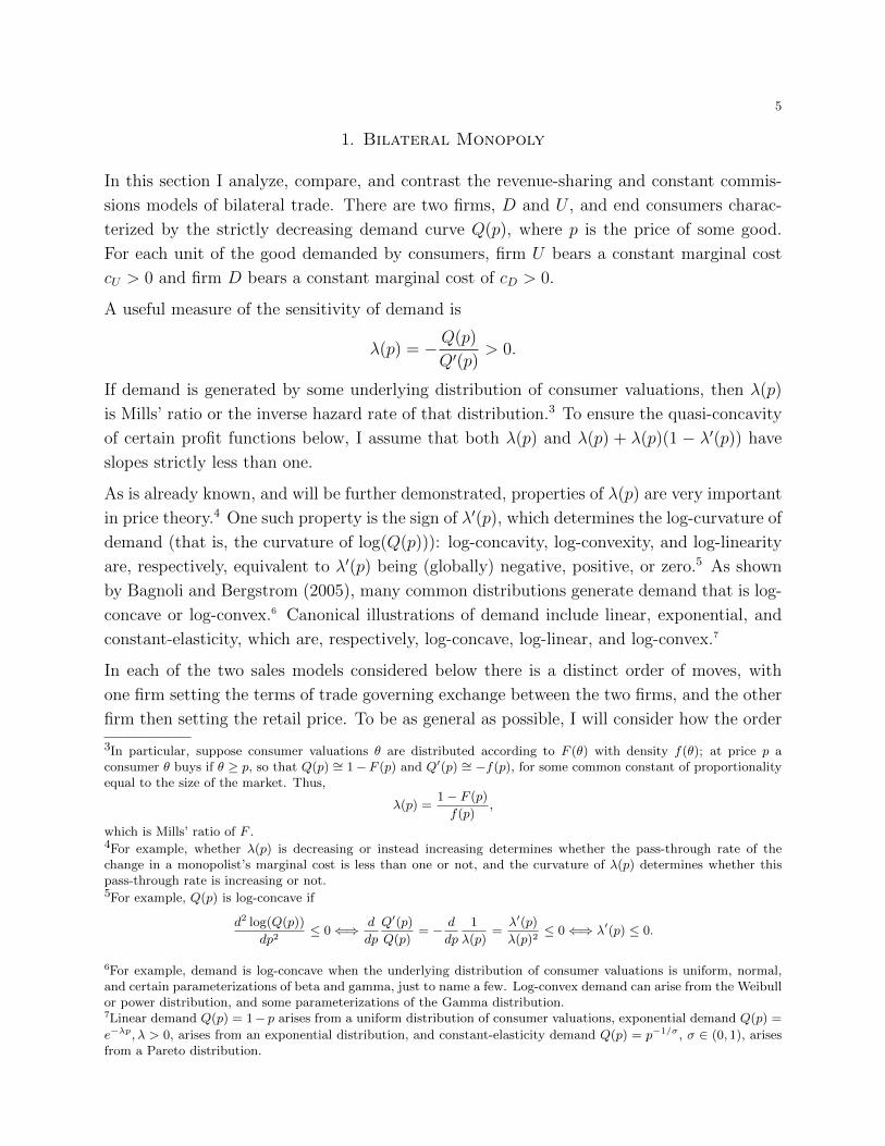
1. Bilateral Monopoly

In this section I analyze, compare, and contrast the revenue-sharing and constant commis-

sions models of bilateral trade. There are two firms, D and U , and end consumers charac-

terized by the strictly decreasing demand curve Q(p), where p is the price of some good.

For each unit of the good demanded by consumers, firm U bears a constant marginal cost

cU > 0 and firm D bears a constant marginal cost of cD > 0.

A useful measure of the sensitivity of demand is

λ(p) = −Q(p)

Q′(p)> 0.

If demand is generated by some underlying distribution of consumer valuations, then λ(p)

is Mills’ ratio or the inverse hazard rate of that distribution.3 To ensure the quasi-concavity

of certain profit functions below, I assume that both λ(p) and λ(p) + λ(p)(1 − λ′(p)) have

slopes strictly less than one.

As is already known, and will be further demonstrated, properties of λ(p) are very important

in price theory.4 One such property is the sign of λ′(p), which determines the log-curvature of

demand (that is, the curvature of log(Q(p))): log-concavity, log-convexity, and log-linearity

are, respectively, equivalent to λ′(p) being (globally) negative, positive, or zero.5 As shown

by Bagnoli and Bergstrom (2005), many common distributions generate demand that is log-

concave or log-convex.6 Canonical illustrations of demand include linear, exponential, and

constant-elasticity, which are, respectively, log-concave, log-linear, and log-convex.7

In each of the two sales models considered below there is a distinct order of moves, with

one firm setting the terms of trade governing exchange between the two firms, and the other

firm then setting the retail price. To be as general as possible, I will consider how the order

3In particular, suppose consumer valuations θ are distributed according to F (θ) with density f(θ); at price p aconsumer θ buys if θ ≥ p, so that Q(p) ∼= 1−F (p) and Q′(p) ∼= −f(p), for some common constant of proportionalityequal to the size of the market. Thus,

λ(p) =1− F (p)

f(p),

which is Mills’ ratio of F .4For example, whether λ(p) is decreasing or instead increasing determines whether the pass-through rate of thechange in a monopolist’s marginal cost is less than one or not, and the curvature of λ(p) determines whether thispass-through rate is increasing or not.5For example, Q(p) is log-concave if

d2 log(Q(p))

dp2≤ 0⇐⇒ d

dp

Q′(p)

Q(p)= − d

dp

1

λ(p)=λ′(p)

λ(p)2≤ 0⇐⇒ λ′(p) ≤ 0.

6For example, demand is log-concave when the underlying distribution of consumer valuations is uniform, normal,and certain parameterizations of beta and gamma, just to name a few. Log-convex demand can arise from the Weibullor power distribution, and some parameterizations of the Gamma distribution.7Linear demand Q(p) = 1− p arises from a uniform distribution of consumer valuations, exponential demand Q(p) =

e−λp, λ > 0, arises from an exponential distribution, and constant-elasticity demand Q(p) = p−1/σ, σ ∈ (0, 1), arisesfrom a Pareto distribution.

6

of moves—and a change to this order—influences market outcomes, and so it is necessary

to introduce additional notation. To this end, agree that “firm 1” is the firm which sets the

terms of trade, and “firm 2” is the firm that sets the retail price, with marginal costs c1

and c2, respectively. Thus, for example, under the typical wholesale model, firm 1 is U with

marginal cost c1 = cU and firm 2 is D with marginal cost c2 = cD. In contrast, under the

typical agency model, firm 1 is D with marginal cost c1 = cD and firm 2 is U with marginal

cost c2 = cU .

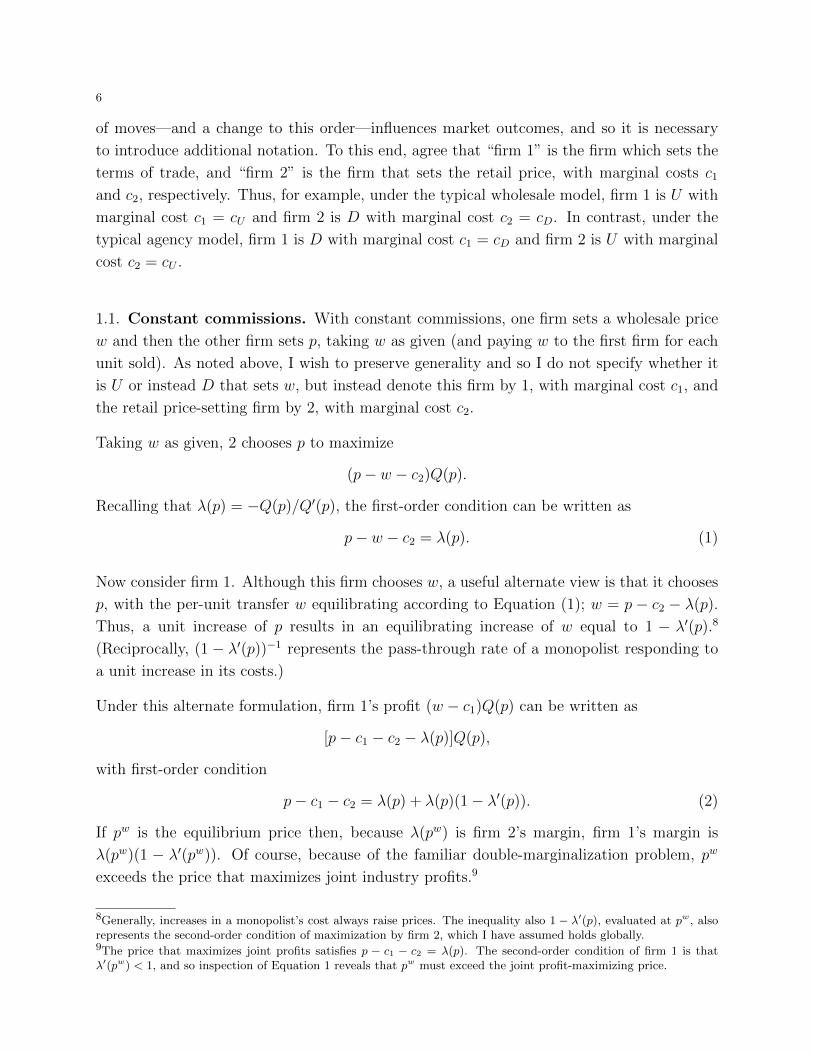
1.1. Constant commissions. With constant commissions, one firm sets a wholesale price

w and then the other firm sets p, taking w as given (and paying w to the first firm for each

unit sold). As noted above, I wish to preserve generality and so I do not specify whether it

is U or instead D that sets w, but instead denote this firm by 1, with marginal cost c1, and

the retail price-setting firm by 2, with marginal cost c2.

Taking w as given, 2 chooses p to maximize

(p− w − c2)Q(p).

Recalling that λ(p) = −Q(p)/Q′(p), the first-order condition can be written as

p− w − c2 = λ(p). (1)

Now consider firm 1. Although this firm chooses w, a useful alternate view is that it chooses

p, with the per-unit transfer w equilibrating according to Equation (1); w = p − c2 − λ(p).

Thus, a unit increase of p results in an equilibrating increase of w equal to 1 − λ′(p).8

(Reciprocally, (1− λ′(p))−1 represents the pass-through rate of a monopolist responding to

a unit increase in its costs.)

Under this alternate formulation, firm 1’s profit (w − c1)Q(p) can be written as

[p− c1 − c2 − λ(p)]Q(p),

with first-order condition

p− c1 − c2 = λ(p) + λ(p)(1− λ′(p)). (2)

If pw is the equilibrium price then, because λ(pw) is firm 2’s margin, firm 1’s margin is

λ(pw)(1 − λ′(pw)). Of course, because of the familiar double-marginalization problem, pw

exceeds the price that maximizes joint industry profits.9

8Generally, increases in a monopolist’s cost always raise prices. The inequality also 1 − λ′(p), evaluated at pw, alsorepresents the second-order condition of maximization by firm 2, which I have assumed holds globally.9The price that maximizes joint profits satisfies p − c1 − c2 = λ(p). The second-order condition of firm 1 is thatλ′(pw) < 1, and so inspection of Equation 1 reveals that pw must exceed the joint profit-maximizing price.

7

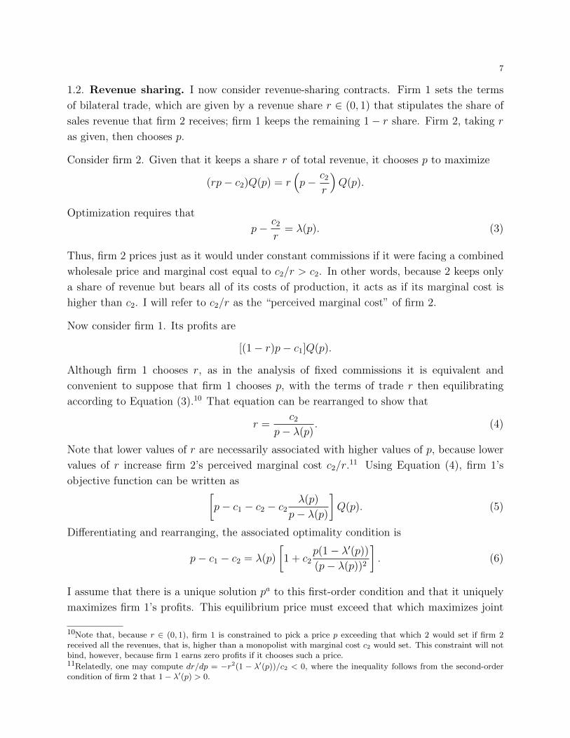
1.2. Revenue sharing. I now consider revenue-sharing contracts. Firm 1 sets the terms

of bilateral trade, which are given by a revenue share r ∈ (0, 1) that stipulates the share of

sales revenue that firm 2 receives; firm 1 keeps the remaining 1− r share. Firm 2, taking r

as given, then chooses p.

Consider firm 2. Given that it keeps a share r of total revenue, it chooses p to maximize

(rp− c2)Q(p) = r(p− c2

r

)Q(p).

Optimization requires that

p− c2

r= λ(p). (3)

Thus, firm 2 prices just as it would under constant commissions if it were facing a combined

wholesale price and marginal cost equal to c2/r > c2. In other words, because 2 keeps only

a share of revenue but bears all of its costs of production, it acts as if its marginal cost is

higher than c2. I will refer to c2/r as the “perceived marginal cost” of firm 2.

Now consider firm 1. Its profits are

[(1− r)p− c1]Q(p).

Although firm 1 chooses r, as in the analysis of fixed commissions it is equivalent and

convenient to suppose that firm 1 chooses p, with the terms of trade r then equilibrating

according to Equation (3).10 That equation can be rearranged to show that

r =c2

p− λ(p). (4)

Note that lower values of r are necessarily associated with higher values of p, because lower

values of r increase firm 2’s perceived marginal cost c2/r.11 Using Equation (4), firm 1’s

objective function can be written as[p− c1 − c2 − c2

λ(p)

p− λ(p)

]Q(p). (5)

Differentiating and rearranging, the associated optimality condition is

p− c1 − c2 = λ(p)

[1 + c2

p(1− λ′(p))(p− λ(p))2

]. (6)

I assume that there is a unique solution pa to this first-order condition and that it uniquely

maximizes firm 1’s profits. This equilibrium price must exceed that which maximizes joint

10Note that, because r ∈ (0, 1), firm 1 is constrained to pick a price p exceeding that which 2 would set if firm 2received all the revenues, that is, higher than a monopolist with marginal cost c2 would set. This constraint will notbind, however, because firm 1 earns zero profits if it chooses such a price.11Relatedly, one may compute dr/dp = −r2(1 − λ′(p))/c2 < 0, where the inequality follows from the second-ordercondition of firm 2 that 1− λ′(p) > 0.

8

profits. To see this, note that the second-order condition of firm 2 is that λ′(pa) < 1, and so

inspection of Equation (6) immediately implies this fact.12

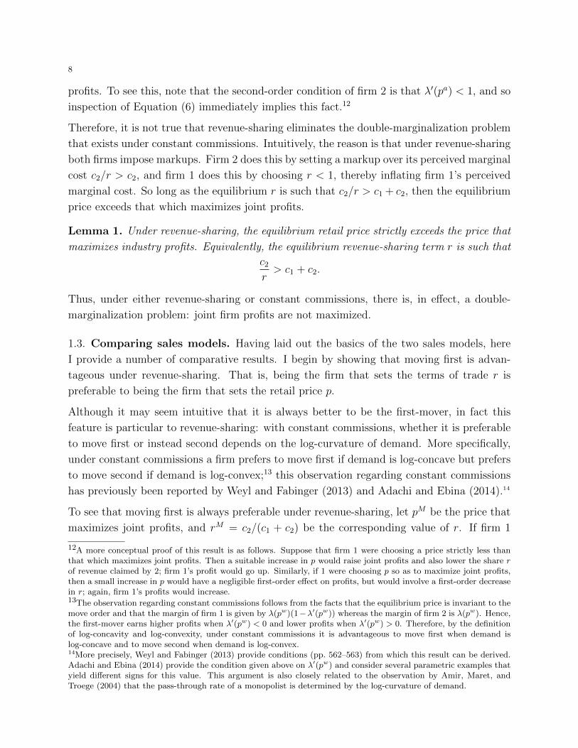
Therefore, it is not true that revenue-sharing eliminates the double-marginalization problem

that exists under constant commissions. Intuitively, the reason is that under revenue-sharing

both firms impose markups. Firm 2 does this by setting a markup over its perceived marginal

cost c2/r > c2, and firm 1 does this by choosing r < 1, thereby inflating firm 1’s perceived

marginal cost. So long as the equilibrium r is such that c2/r > c1 + c2, then the equilibrium

price exceeds that which maximizes joint profits.

Lemma 1. Under revenue-sharing, the equilibrium retail price strictly exceeds the price that

maximizes industry profits. Equivalently, the equilibrium revenue-sharing term r is such that

c2

r> c1 + c2.

Thus, under either revenue-sharing or constant commissions, there is, in effect, a double-

marginalization problem: joint firm profits are not maximized.

1.3. Comparing sales models. Having laid out the basics of the two sales models, here

I provide a number of comparative results. I begin by showing that moving first is advan-

tageous under revenue-sharing. That is, being the firm that sets the terms of trade r is

preferable to being the firm that sets the retail price p.

Although it may seem intuitive that it is always better to be the first-mover, in fact this

feature is particular to revenue-sharing: with constant commissions, whether it is preferable

to move first or instead second depends on the log-curvature of demand. More specifically,

under constant commissions a firm prefers to move first if demand is log-concave but prefers

to move second if demand is log-convex;13 this observation regarding constant commissions

has previously been reported by Weyl and Fabinger (2013) and Adachi and Ebina (2014).14

To see that moving first is always preferable under revenue-sharing, let pM be the price that

maximizes joint profits, and rM = c2/(c1 + c2) be the corresponding value of r. If firm 1

12A more conceptual proof of this result is as follows. Suppose that firm 1 were choosing a price strictly less thanthat which maximizes joint profits. Then a suitable increase in p would raise joint profits and also lower the share rof revenue claimed by 2; firm 1’s profit would go up. Similarly, if 1 were choosing p so as to maximize joint profits,then a small increase in p would have a negligible first-order effect on profits, but would involve a first-order decreasein r; again, firm 1’s profits would increase.13The observation regarding constant commissions follows from the facts that the equilibrium price is invariant to themove order and that the margin of firm 1 is given by λ(pw)(1−λ′(pw)) whereas the margin of firm 2 is λ(pw). Hence,the first-mover earns higher profits when λ′(pw) < 0 and lower profits when λ′(pw) > 0. Therefore, by the definitionof log-concavity and log-convexity, under constant commissions it is advantageous to move first when demand islog-concave and to move second when demand is log-convex.14More precisely, Weyl and Fabinger (2013) provide conditions (pp. 562–563) from which this result can be derived.Adachi and Ebina (2014) provide the condition given above on λ′(pw) and consider several parametric examples thatyield different signs for this value. This argument is also closely related to the observation by Amir, Maret, andTroege (2004) that the pass-through rate of a monopolist is determined by the log-curvature of demand.

9

chose to implement pM , the industry profit margin would be pM − c1− c2 = λ(pM), and firm

1’s profits would be

[(1− rM)pM − c1]Q(pM) =

[c1

c1 + c2

(c1 + c2 + λ(pM))− c1

]Q(pM) =

c1

c1 + c2

λ(pM)Q(pM).

Thus, firm 1 could ensure itself a fraction c1/(c1+c2) of maximized industry profits. However,

from Lemma 1, it is optimal for firm 1 to chose a strictly higher price (and hence a lower

value of r), and thereby earn strictly higher profits: in equilibrium, firm 1 earns strictly

more than a share c1/(c1 + c2) of maximized industry profits. In turn, this means that for

any particular firm i ∈ D,U, under revenue-sharing i must earn higher profit if it moves

first than if it moves second. For example, if U moves first it will claim more than a share

cU/(cD + cU) of maximized industry profits, and if instead D moves first then U will secure

less than a share 1− cD/(cD + cU) = cU/(cD + cU) of these profits.

Proposition 1. Under revenue-sharing, each firm prefers to be the first-mover. In contrast,

with constant commissions each firm prefers to be the first-mover if demand is log-concave

but prefers to be the second-mover if demand is log-convex.

Proposition 1 confirms that the desire to set the terms of trade is particularly alluring under

revenue-sharing, holding regardless of the shape of demand. I note again that the result on

move order under constant commissions is already known (see Weyl and Fabinger (2013)

and Adachi and Ebina (2014)); my contribution pertains to revenue-sharing.15

I now assess the effect of revenue-sharing on the retail price. Although Lemma 1 indicates

that revenue-sharing does not eliminate the double-marginalization problem, it turns out

that under a certain condition on demand this pricing externality is nonetheless mitigated.

This condition involves the elasticity of λ(p), which is also the elasticity of Mills’ ratio of the

underlying distribution of consumer valuations, given by pλ′(p)/λ(p).16

Proposition 2. If the elasticity of Mills ratio is less than one (pλ′(p)/λ(p) ≤ 1), then

the equilibrium retail price under revenue-sharing is strictly less than that under constant

commissions (pa < pw). This result holds even if the move order differs depending on

whether constant commissions or revenue-sharing is used.

As I discuss in more detail below, the condition that pλ′(p)/λ(p) ≤ 1 is satisfied so long

as demand is not “too convex.” It is satisfied for all log-concave and log-linear demand

functions as well as constant-elasticity demand.

15Note that Proposition 1 does not say that firm 1 earns higher profits than firm 2, but merely that moving first isbetter than moving second. This is in contrast to the case with constant commissions. The reason for the differenceis that, under revenue-sharing, the equilibrium retail price may depend on which firm sets the terms, so that grossprofits may depend on the move order.16Recall that Mills’ ratio equals (1− F (θ))/f(θ), where F is the underlying distribution of consumer valuations andf is the corresponding density function. The Mills’ ratio is also called the inverse hazard rate.

10

Proposition 2 is interesting because the goal of firm 1 is not to raise consumer surplus.

Indeed, this profit motive implies that firm 1 may face a tradeoff when choosing p under the

two sales models. On the one hand, the optimality condition for firm 2 (Equation (3)) implies

that firm 2 receives a margin of only rλ(p) under revenue-sharing rather than λ(p) under

constant commissions. Thus, the margin of firm 1 is higher for any given p, encouraging firm

1 to induce a lower price. On the other hand, under revenue-sharing an increase in p may

raise the margin that firm 1 receives by more than it raises the margin that it receives under

constant commissions. This force encourages firm 1 to set a higher price.

To see this second effect, suppose that demand has a constant elasticity (so that λ(p) = σp

for σ ∈ (0, 1)) and note that for arbitrary p firm 1’s margin under constant commissions is

p − c1 − c2 − λ(p) = (1 − σ)p − c1 − c2; raising p raises firm 1’s margin by 1 − σ < 1. In

contrast, under revenue-sharing, firm 1’s margin is p− c1 − c2 − rλ(p). Using the fact (from

Equation (4)) that r = c2/(p− λ(p)) = c2/(1− σ)p, firm 1’s margin is

p− c1 − c2 − c2σ

1− σ.

Thus, increasing p by one raises firm 1’s margin by one—from this perspective, a price

increase is more attractive under revenue-sharing.17 Despite this tradeoff, the overall effect

of revenue-sharing is to decrease the retail price.18 A related intuition follows Proposition 3.

Note that the sufficient condition pλ′(p) ≤ λ(p) from Proposition 2 readily admits some

log-convex demand functions (most obviously the constant-elasticity one), in addition to

log-linear and log-concave ones. Indeed, rewriting the elasticity of Mills’ ratio in terms of

the underlying demand function Q(p), the above condition is equivalent to

pQ′(p)

Q(p)− pQ′′(p)

Q′(p)≤ 1.

The left-hand side is the difference between the elasticity of demand and the elasticity of the

slope of demand (this second term is also called the adjusted-concavity of demand), and the

condition for log-concavity is that this is less than zero. Thus, the condition clearly admits

some log-convex demand functions.

I now explore how a move to revenue-sharing influences the profitability of the firms, sup-

posing that the same firm that sets the terms of trade under constant commissions also sets

17Put instead in terms of traditional pass-through concepts, this says that increasing firm 1’s margin by one leadsto an increase in p of 1/(1 − σ) > 1 under constant commissions, whereas increasing firm 1’s margin by one leadsto an increase in p of only one under revenue-sharing. In this second sense, there is complete pass-through underrevenue-sharing, but more-than-complete pass-through with constant commissions.18When demand exhibits constant elasticity, both pw and pa can be explicitly solved for, using the optimality condi-tions in Equations (2) and (6). This yields

pa =(1− σ)c1 + c2

(1− σ)2<

c1 + c2(1− σ)2

= pw.

11

them under revenue-sharing. As I discuss in detail below, the taxation literature already

suggests an answer to how firm 1’s profits will change, but does not provide insight into how

firm 2’s profits will. Regardless, I significantly generalize these results in the next section

where I consider bilateral imperfect competition.

Proposition 3. Suppose that the order in which firms D and U move is the same under

revenue-sharing as under constant commissions (so that the identities of firm 1 and firm 2

are the same under either sales model). Then:

(1) Firm 1 earns higher profits under revenue-sharing than under constant commissions,

(2) Firm 2 earns lower profits under revenue-sharing than under constant commissions

if demand is either log-linear (λ(p) = λ > 0 for each p) or constant-elasticity.

It may seem surprising that firm 2 can be worse off, especially given that industry profits are

higher under revenue-sharing. But in another sense, it is not surprising: firm 1 is seeking to

maximize its own profits, not those of firm 2.

Note that the log-linear case is a natural one to consider, because with constant commissions

firm 1 and firm 2 receive equal profits in equilibrium; neither firm has an advantage over the

other. But even with log-concave demand firm 2 can be worse off under revenue-sharing.

This is notable because log-concavity implies that firm 2 is at a disadvantage to firm 1 under

constant commissions, as shown in Proposition 1, and so one might have thought that firm

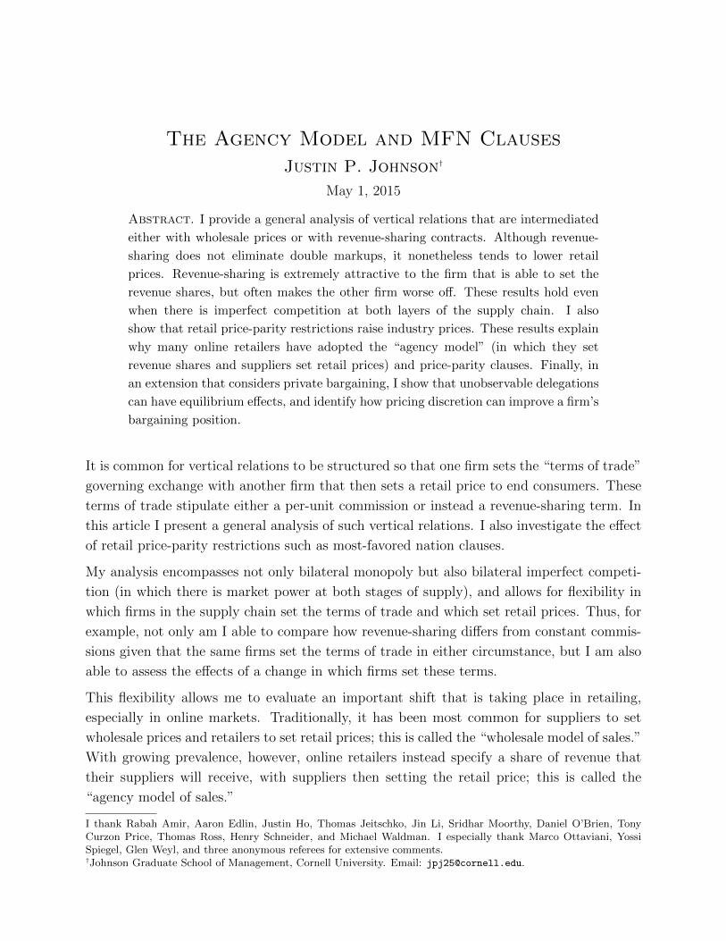
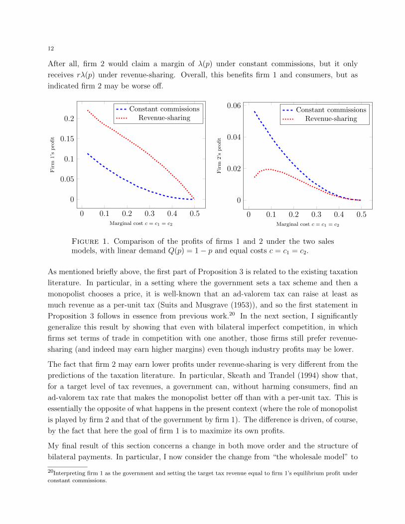
2 would tend to prefer revenue-sharing. To see that is not so, suppose that demand is linear,

Q(p) = 1 − p, and firms have equal costs, c1 = c2 = c. For the range of costs that lead

to positive equilibrium output (that is, c < 1/2), the profits of firm 2 under the two sales

models are shown in the right-hand panel of Figure 1; the left-hand panel of that figure

illustrates the profits of firm 1.19

An intuition for Proposition 3 emerges from an understanding of a fundamental difference

between the two sales models, which is that revenue-sharing reduces the incentives of firm 2

to increase its per-unit margin. To see this, note that under constant commissions firm 2’s

margin is p − w − c2 so that if it increases p by one it also raises its margin by one; firm 2

captures the entirety of its increase in the price. In contrast, under revenue-sharing firm 2’s

margin is rp − c2 so that an increase in p raises its margin by only r < 1; firm 2 captures

only a fraction of the increase in p, with firm 1 capturing the rest.

The fact that revenue-sharing makes price increases less attractive for firm 2 is exploited by

firm 1 in its selection of the revenue-sharing term r. Closely related is the fact that at any

given p firm 1 must be earning a higher margin than it would under constant commissions.

19To be precise, this figure illustrates profits for firm 1 and firm 2, under the assumption that the same firm i ∈ D,Umoves first under both constant commissions and revenue-sharing. Also note that although linear demand is log-concave, log-concave demand by itself does not guarantee that firm 2 is worse off under revenue sharing.

12

After all, firm 2 would claim a margin of λ(p) under constant commissions, but it only

receives rλ(p) under revenue-sharing. Overall, this benefits firm 1 and consumers, but as

indicated firm 2 may be worse off.

0 0.1 0.2 0.3 0.4 0.5

0

0.05

0.1

0.15

0.2

Marginal cost c = c1 = c2

Fir

m1’s

pro

fit

Constant commissionsRevenue-sharing

0 0.1 0.2 0.3 0.4 0.5

0

0.02

0.04

0.06

Marginal cost c = c1 = c2F

irm

2’s

pro

fit

Constant commissionsRevenue-sharing

Figure 1. Comparison of the profits of firms 1 and 2 under the two salesmodels, with linear demand Q(p) = 1− p and equal costs c = c1 = c2.

As mentioned briefly above, the first part of Proposition 3 is related to the existing taxation

literature. In particular, in a setting where the government sets a tax scheme and then a

monopolist chooses a price, it is well-known that an ad-valorem tax can raise at least as

much revenue as a per-unit tax (Suits and Musgrave (1953)), and so the first statement in

Proposition 3 follows in essence from previous work.20 In the next section, I significantly

generalize this result by showing that even with bilateral imperfect competition, in which

firms set terms of trade in competition with one another, those firms still prefer revenue-

sharing (and indeed may earn higher margins) even though industry profits may be lower.

The fact that firm 2 may earn lower profits under revenue-sharing is very different from the

predictions of the taxation literature. In particular, Skeath and Trandel (1994) show that,

for a target level of tax revenues, a government can, without harming consumers, find an

ad-valorem tax rate that makes the monopolist better off than with a per-unit tax. This is

essentially the opposite of what happens in the present context (where the role of monopolist

is played by firm 2 and that of the government by firm 1). The difference is driven, of course,

by the fact that here the goal of firm 1 is to maximize its own profits.

My final result of this section concerns a change in both move order and the structure of

bilateral payments. In particular, I now consider the change from “the wholesale model” to

20Interpreting firm 1 as the government and setting the target tax revenue equal to firm 1’s equilibrium profit underconstant commissions.

13

“the agency model.” Recall that this corresponds to moving from a situation where firm U

sets w and D sets p, to one where D sets r and U sets p.

Proposition 4. If demand is log-concave, log-linear, or constant-elasticity, then a shift from

the wholesale model to the agency model raises the profits of D but lowers the profits of U .

This proposition, along with its generalization to bilateral imperfect competition in the

next section, provides an explanation for why online firms such as Amazon and eBay may be

switching to the agency model, and also of course suggests suppliers need not be beneficiaries

of this change. Indeed, this result is somewhat stronger than stated, as is readily apparent

from inspection of the proof: so long as pλ′(p) ≤ λ(p), U is harmed by the move to the

agency model.21 Indeed, log-convex demand satisfying this condition emphasizes the strong

effects of moving to the agency model: even though U earns lower profits than D does under

the wholesale model when demand is log-convex, U nonetheless prefers the wholesale model

to the agency model—revenue sharing is too powerful a weapon in the hands of D.

2. Bilateral Imperfect Competition

In this section I extend the model and analysis above to a setting in which there is competition

at both layers of the supply chain.22 Rather than specify any particular model of such

competition, I take an approach based on conduct parameters similar to that in the study of

pass-through under constant commissions by Weyl and Fabinger (2013).23 This allows my

results to be stated in terms of properties of the aggregate demand function in the industry,

thus providing a close analogue to the study of bilateral monopoly above.

Given the work above, it is easier here to adopt an approach that is slightly more compact.

Let Q(p) denote the aggregate demand of consumers, where the interpretation is that each

of M substitute products is sold at common price p by each of N substitute retailers. As

before, λ(p) = −Q(p)/Q′(p). All derivatives in this section measure the effect of an increase

in the common price p of the retail prices of all products sold through all stores. Thus, Q′(p)

measures the effect on aggregate demand from a small increase in all prices.

My analysis proceeds as follows. First I specify how layer two reacts to arbitrary terms of

trade r or w, that is, which retail price p is set by the second layer given such terms of trade.

21As noted earlier, the condition that pλ′(p)/λ(p) ≤ 1 covers log-linear and log-concave demand as well as somelog-convex demand functions such as the constant-elasticity one.22Related work that considers market power at multiple stages of production includes Salinger (1988), Reisinger andSchnitzer (2010), and Kourandi and Vettas (2012), consider models that feature both intermediate and final goodsmarkets in their investigations of vertical structure.23In an earlier draft of this paper, I specified a complete micro-foundation for such competition, and showed thatmoving from the wholesale model to the agency model could lower retail prices, yet also make the downstream firmsbetter off at the expense of upstream firms. A downside of that model was that only very limited forms of demandcould tractably be considered. In particular, that model effectively assumed pass-through rates equal to unity.

14

Second, I specify how the first layer determines these terms of trade, taking as given the

response of the second layer.

Suppose that the terms of trade have been set by the first layer. Let m2(p) denote the per-

unit margin of the second layer, given that all firms of that layer are setting the same price p.

For example, under constant commissions m2(p) = p−w−c2 whereas under revenue-sharing

m2(p) = rp− c2. The aggregate profit of the second layer is

m2(p)Q(p),

with derivative

m′2(p)Q(p) +m2(p)Q′(p).

For arbitrary r or w, I define the value of p set by layer 2 to be that which implicitly solves

m2(p)

m′2(p)= θ2λ(p) =⇒ m2(p) = θ2m

′2(p)λ(p), (7)

where θ2 ∈ (0, 1) is the conduct parameter of layer 2. Computing the appropriate derivatives

m′2(p), under constant commissions this says that m2(p) = p − w − c2 = θ2λ(p) whereas

under revenue-sharing (and using m′2(p) = r) this says that m2(p) = rp− c2 = θ2rλ(p).

Note that if θ2 = 1 then these equations are precisely what was derived earlier for the optimal

response of firm 2 in the case of bilateral monopoly (see Equations (1) and (3)). On the other

hand, if θ2 = 0 then these margins are zero. Thus, varying θ2 spans the range of outcomes

from perfect competition in layer 2 to perfectly collusive behavior in layer 2.

Now consider the profits of layer 1. As before, it can be supposed that this layer sets p, with

the terms of trade with layer 2 then equilibrating. For any final price p, the per-unit margin

of layer 1 is denoted by m1, and satisfies

m1(p) = p− c1 − c2 − m2(p), (8)

where m2(p) is the margin that layer 2 must be receiving. From the work above, for a given

p the margin of the second layer is m2(p) = θ2λ(p) under constant commissions. Under

revenue-sharing this margin is θ2rλ(p), but using the equilibrium condition given just above

for layer 2 (that rp− c2 = θ2rλ(p)), r is given by

r =c2

p− θ2λ(p),

a close analogue to Equation (4). Thus eliminating r, under revenue-sharing

m2(p) =θ2c2λ(p)

p− θ2λ(p).

For arbitrary p, the overall profitability of the first layer is simply m1(p)Q(p), with derivative

m′1(p)Q(p) +m1(p)Q′(p).

15

I define the equilibrium value of p to be that which satisfies

m1(p)

m′1(p)= θ1λ(p) =⇒ m1(p) = θ1m

′1(p)λ(p). (9)

As θ1 ranges from zero to one the resulting price p ranges from that which gives layer 1 no

margin to that which maximizes the profits of layer 1, given how layer 2 will respond.

Noting that m′1(p) = 1−m′2(p) (using Equation (8)) and computing the value of m′2(p) under

both constant commissions and revenue-sharing, equations characterizing the industry price

are readily derived. As before, let pw and pa denote the industry prices under the two sales

models. The following lemma summarizes the definitions and work above.

Lemma 2. Under bilateral imperfect competition with conduct parameters θ1 and θ2, the

retail price pw under constant commissions satisfies

pw − c1 − c2 = θ2λ(pw) + θ1λ(pw)(1− θ2λ′(pw)), (10)

and the retail price pa under revenue-sharing satisfies

pa − c1 − c2 = θ1λ(pa) + θ2c2λ(pa)

[pa(1− θ1λ

′(p)) + λ(p)(θ1 − θ2)

(pa − θ2λ(pa))2

]. (11)

If θ1 = θ2 = 1, these equations reduce to those derived for the bilateral monopoly case

(Equations (2) and (6)). And, for θ1 = θ2 = 0, both of these industry margins equal zero.

Finally, note that pw is, once again, independent of which firm moves first, as can be seen

by expanding the right-hand side of Equation (10).

I will now show that, under broadly similar conditions on the shape of demand, key results

derived for bilateral monopoly continue to hold under bilateral competition.

Proposition 5. Under bilateral imperfect competition, if the elasticity of Mills ratio is less

than one (pλ′(p)/λ(p) ≤ 1), then the equilibrium retail price under revenue-sharing is strictly

less than that under constant commissions (pa < pw). This result holds even if the move order

differs depending on whether constant commissions or revenue-sharing is used.

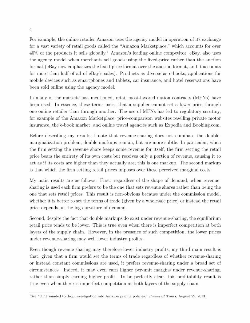
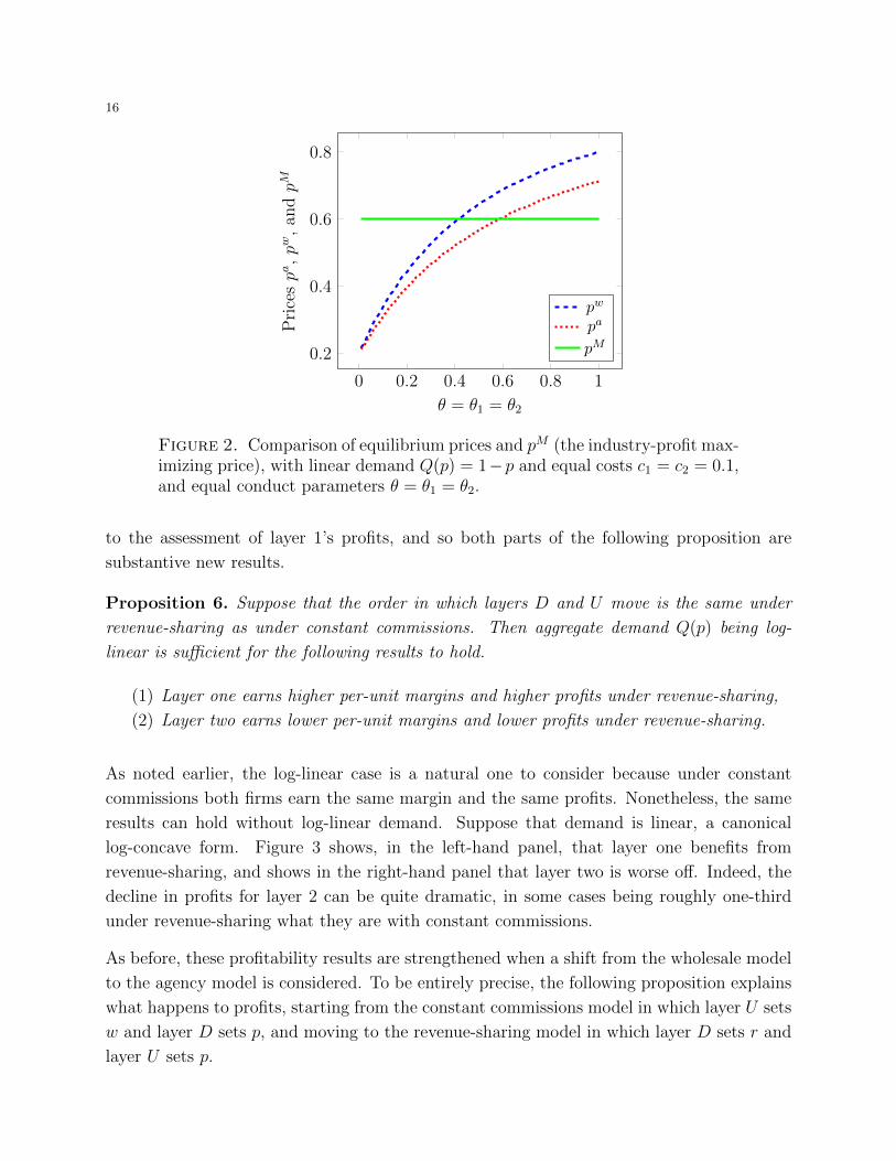
Recall that in the bilateral monopoly case a move to revenue-sharing lowers the retail price,

which moves it closer to the price pM that maximizes industry profits. In contrast, with

bilateral imperfect competition, such a price reduction may lower industry profits. The

reason is simply that, depending on the conduct parameters, pw may be lower than pM , so

that a further reduction is bad for these profits. This possibility can be seen clearly in Figure

2, which graphs equilibrium prices in comparison to pM for a linear-demand specification.

Strikingly, even if industry profits decrease, revenue-sharing nonetheless tends to benefit

layer 1 and harm layer 2. Note that because there is competition amongst both layers, the

classic result from the taxation literature (Suits and Musgrave (1953)) no longer applies

16

0 0.2 0.4 0.6 0.8 1

0.2

0.4

0.6

0.8

θ = θ1 = θ2

Pri

cespa

,pw

,an

dpM

pw

pa

pM

Figure 2. Comparison of equilibrium prices and pM (the industry-profit max-imizing price), with linear demand Q(p) = 1−p and equal costs c1 = c2 = 0.1,and equal conduct parameters θ = θ1 = θ2.

to the assessment of layer 1’s profits, and so both parts of the following proposition are

substantive new results.

Proposition 6. Suppose that the order in which layers D and U move is the same under

revenue-sharing as under constant commissions. Then aggregate demand Q(p) being log-

linear is sufficient for the following results to hold.

(1) Layer one earns higher per-unit margins and higher profits under revenue-sharing,

(2) Layer two earns lower per-unit margins and lower profits under revenue-sharing.

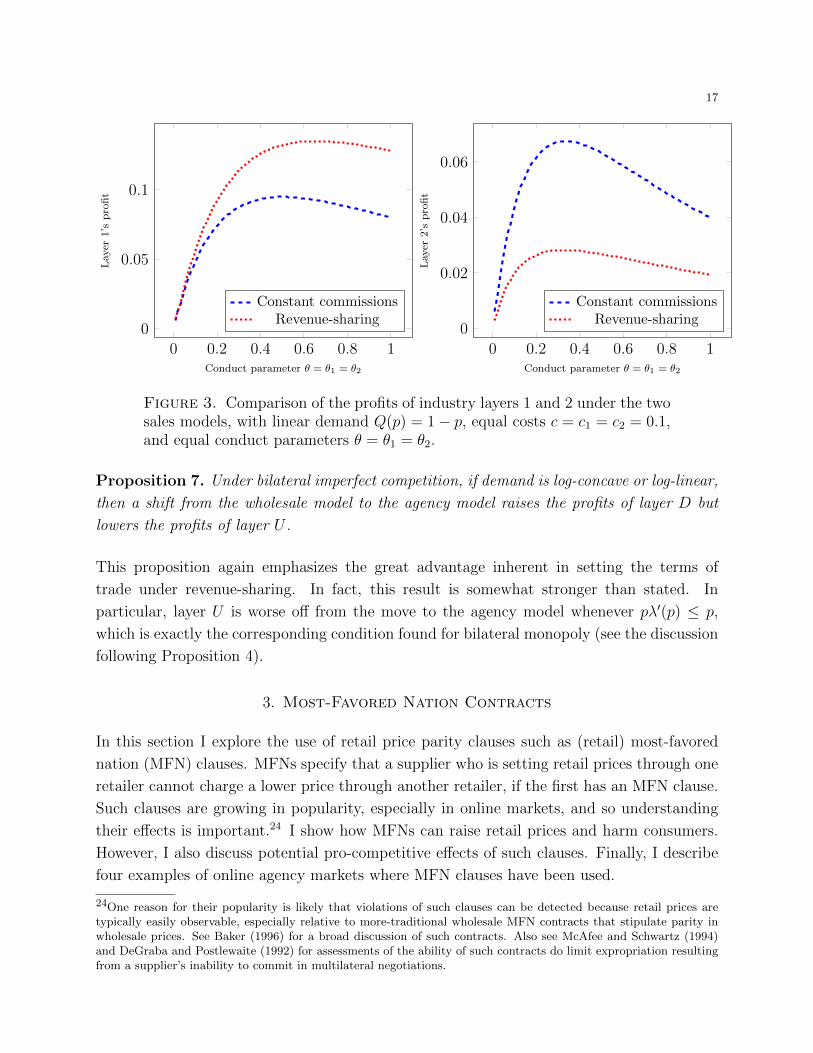
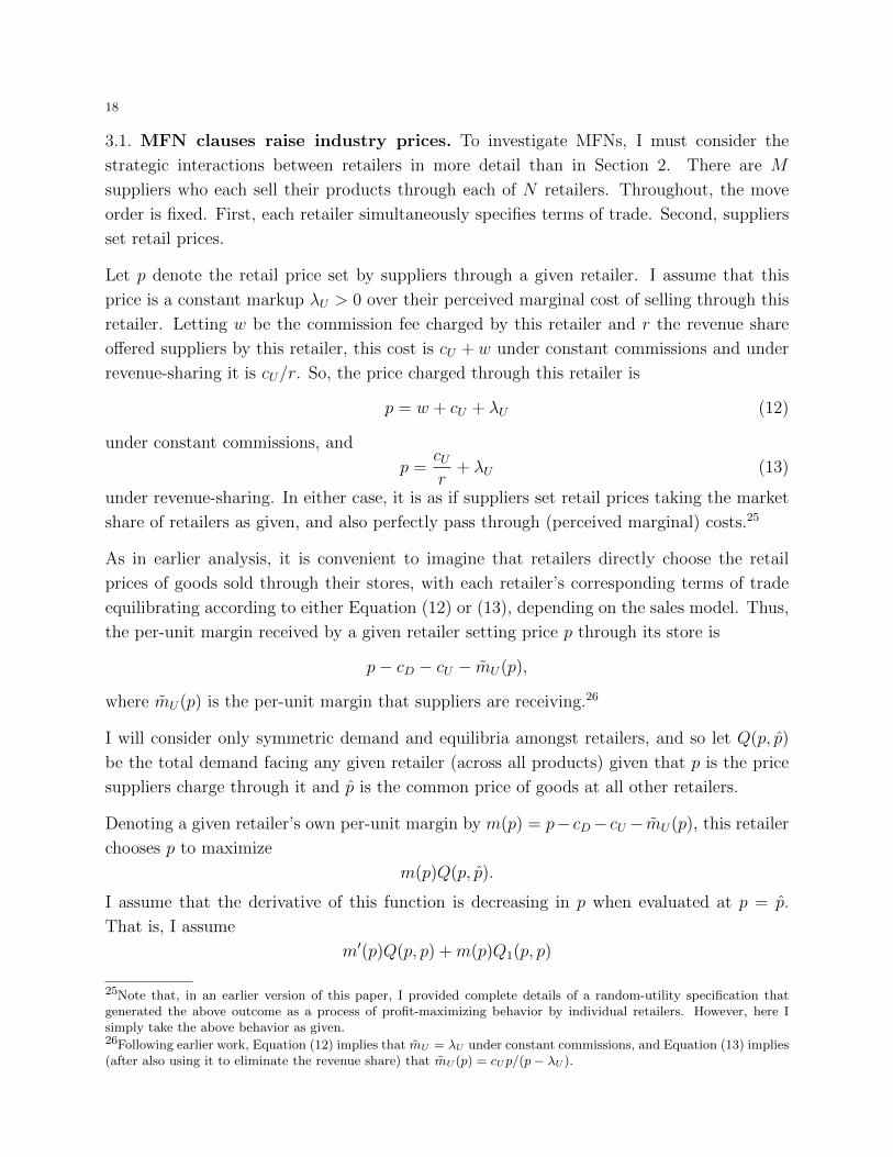
As noted earlier, the log-linear case is a natural one to consider because under constant

commissions both firms earn the same margin and the same profits. Nonetheless, the same

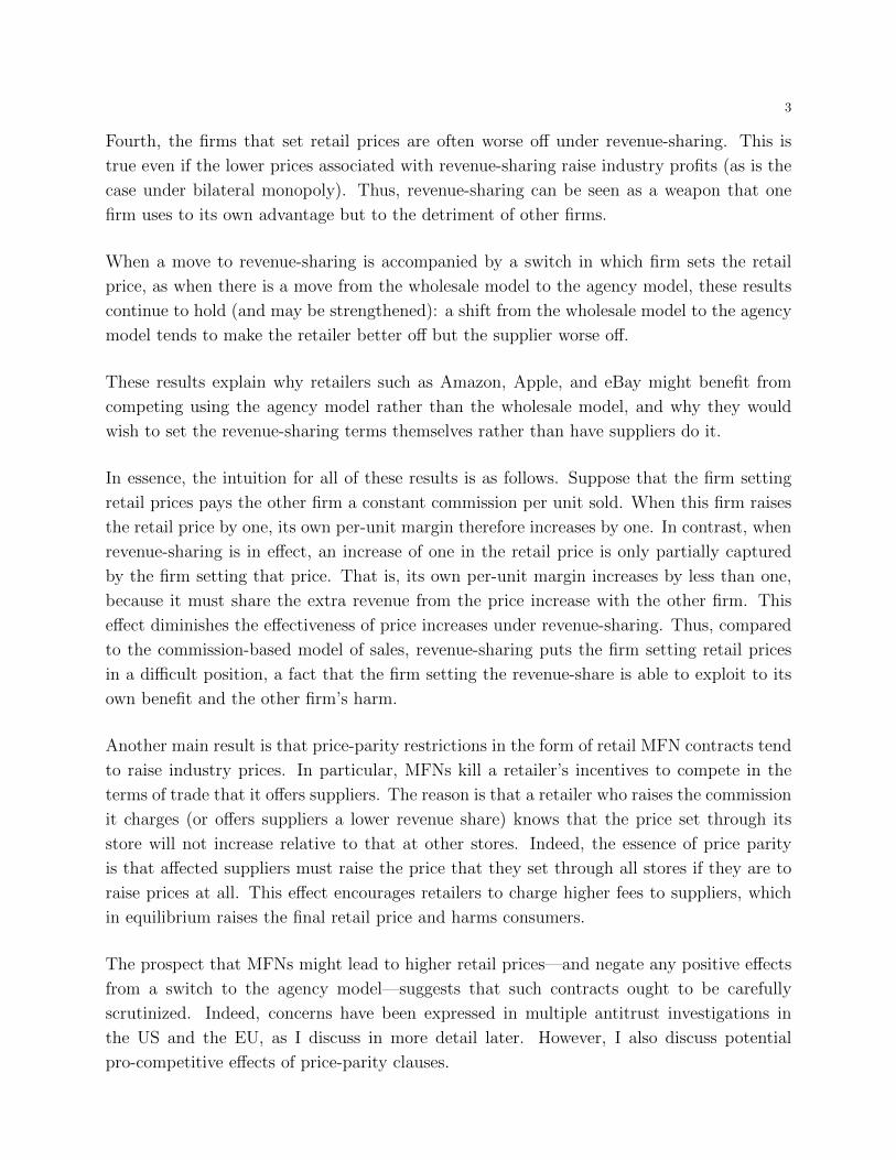
results can hold without log-linear demand. Suppose that demand is linear, a canonical

log-concave form. Figure 3 shows, in the left-hand panel, that layer one benefits from

revenue-sharing, and shows in the right-hand panel that layer two is worse off. Indeed, the

decline in profits for layer 2 can be quite dramatic, in some cases being roughly one-third

under revenue-sharing what they are with constant commissions.

As before, these profitability results are strengthened when a shift from the wholesale model

to the agency model is considered. To be entirely precise, the following proposition explains

what happens to profits, starting from the constant commissions model in which layer U sets

w and layer D sets p, and moving to the revenue-sharing model in which layer D sets r and

layer U sets p.

17

0 0.2 0.4 0.6 0.8 10

0.05

0.1

Conduct parameter θ = θ1 = θ2

Layer

1’s

pro

fit

Constant commissionsRevenue-sharing

0 0.2 0.4 0.6 0.8 1

0

0.02

0.04

0.06

Conduct parameter θ = θ1 = θ2

Layer

2’s

pro

fit

Constant commissionsRevenue-sharing

Figure 3. Comparison of the profits of industry layers 1 and 2 under the twosales models, with linear demand Q(p) = 1− p, equal costs c = c1 = c2 = 0.1,and equal conduct parameters θ = θ1 = θ2.

Proposition 7. Under bilateral imperfect competition, if demand is log-concave or log-linear,

then a shift from the wholesale model to the agency model raises the profits of layer D but

lowers the profits of layer U .

This proposition again emphasizes the great advantage inherent in setting the terms of

trade under revenue-sharing. In fact, this result is somewhat stronger than stated. In

particular, layer U is worse off from the move to the agency model whenever pλ′(p) ≤ p,

which is exactly the corresponding condition found for bilateral monopoly (see the discussion

following Proposition 4).

3. Most-Favored Nation Contracts

In this section I explore the use of retail price parity clauses such as (retail) most-favored

nation (MFN) clauses. MFNs specify that a supplier who is setting retail prices through one

retailer cannot charge a lower price through another retailer, if the first has an MFN clause.

Such clauses are growing in popularity, especially in online markets, and so understanding

their effects is important.24 I show how MFNs can raise retail prices and harm consumers.

However, I also discuss potential pro-competitive effects of such clauses. Finally, I describe

four examples of online agency markets where MFN clauses have been used.

24One reason for their popularity is likely that violations of such clauses can be detected because retail prices aretypically easily observable, especially relative to more-traditional wholesale MFN contracts that stipulate parity inwholesale prices. See Baker (1996) for a broad discussion of such contracts. Also see McAfee and Schwartz (1994)and DeGraba and Postlewaite (1992) for assessments of the ability of such contracts do limit expropriation resultingfrom a supplier’s inability to commit in multilateral negotiations.

18

3.1. MFN clauses raise industry prices. To investigate MFNs, I must consider the

strategic interactions between retailers in more detail than in Section 2. There are M

suppliers who each sell their products through each of N retailers. Throughout, the move

order is fixed. First, each retailer simultaneously specifies terms of trade. Second, suppliers

set retail prices.

Let p denote the retail price set by suppliers through a given retailer. I assume that this

price is a constant markup λU > 0 over their perceived marginal cost of selling through this

retailer. Letting w be the commission fee charged by this retailer and r the revenue share

offered suppliers by this retailer, this cost is cU + w under constant commissions and under

revenue-sharing it is cU/r. So, the price charged through this retailer is

p = w + cU + λU (12)

under constant commissions, and

p =cUr

+ λU (13)

under revenue-sharing. In either case, it is as if suppliers set retail prices taking the market

share of retailers as given, and also perfectly pass through (perceived marginal) costs.25

As in earlier analysis, it is convenient to imagine that retailers directly choose the retail

prices of goods sold through their stores, with each retailer’s corresponding terms of trade

equilibrating according to either Equation (12) or (13), depending on the sales model. Thus,

the per-unit margin received by a given retailer setting price p through its store is

p− cD − cU − mU(p),

where mU(p) is the per-unit margin that suppliers are receiving.26

I will consider only symmetric demand and equilibria amongst retailers, and so let Q(p, p)

be the total demand facing any given retailer (across all products) given that p is the price

suppliers charge through it and p is the common price of goods at all other retailers.

Denoting a given retailer’s own per-unit margin by m(p) = p− cD− cU − mU(p), this retailer

chooses p to maximize

m(p)Q(p, p).

I assume that the derivative of this function is decreasing in p when evaluated at p = p.

That is, I assume

m′(p)Q(p, p) +m(p)Q1(p, p)

25Note that, in an earlier version of this paper, I provided complete details of a random-utility specification thatgenerated the above outcome as a process of profit-maximizing behavior by individual retailers. However, here Isimply take the above behavior as given.26Following earlier work, Equation (12) implies that mU = λU under constant commissions, and Equation (13) implies(after also using it to eliminate the revenue share) that mU (p) = cUp/(p− λU ).

19

is decreasing in p. The price at which it equals zero corresponds to the equilibrium price for

the relevant sales model.

Although the goal of this section is to investigate MFN clauses, the model specified here also

returns outcomes familiar from earlier analysis. In particular, under the conditions already

given, the equilibrium price under revenue-sharing is less than that under constant commis-

sions. If additionally −Q(p, p)/Q1(p, p) is decreasing, then retailers earn higher margins and

higher profits under revenue-sharing, and suppliers earn lower margins. I demonstrate these

claims in the appendix. Thus, the model is quite similar to those analyzed earlier, but allows

for precisely defined strategic interactions among competing retailers so that the effect of

price-parity restrictions can be rigorously assessed.

Suppose industry-wide MFNs are in effect. This means that the price suppliers set through

a given retailer must be the same as the price they set through all other retailers, even if the

terms of trade differ across retailers. This influences the incentives retailers face when they

set terms of trade. In particular, if a retailer raises the commission w it charges suppliers

or offers suppliers a lower revenue share r, suppliers will respond by raising the retail prices

charged through all retailers, not just those charged through this retailer.27

Proposition 8. MFN clauses raise industry prices. This is true whether constant-commissions

or instead revenue-sharing is in effect (and MFNs raise the equilibrium wholesale price w

charged to suppliers or lower the share of revenue r that suppliers receive, respectively).

The intuition is as follows. With MFNs, when a retailer offers suppliers less-attractive terms

of trade, it does so with the knowledge that the resulting retail prices will not place it at

a relative disadvantage compared to other retailers; there will be retail price parity. This

encourages retailers to either raise w or lower r, which raises the perceived marginal costs of

suppliers and in turn raises industry prices.

3.2. Possible pro-competitive effects of MFNs. Although the analysis above indicates

how MFNs may raise prices and harm consumers, it is not hard to imagine how MFNs might

also be pro-competitive. For example, MFNs might encourage investments.

This force seems particularly relevant for markets where the retail landscape is changing

rapidly. In particular, many new online retailers have appeared in recent years, and some

of them have chosen to use price-parity restrictions. Some of these retailers have faced

substantial costs of developing their online platforms, and it is possible that price-parity

restrictions have encouraged their entry and, potentially, benefitted consumers.

Related, price-parity restrictions may also have pro-competitive effects if they encourage

efficient investments among retailers and suppliers. For example, suppose that there were

27When MFNs are in effect, I suppose suppliers set prices so that their average markup is λU .

20

a single vertically integrated supplier and a single independent retailer. If the independent

retailer must make investments that benefit the supplier, the incentives for such incentives

may be blunted if the supplier undercuts the retailer through its own retail outlet. A price-

parity agreement may prevent such behavior and possibly benefit consumers.

3.3. Antitrust cases. In this section I describe four markets in which retail price parity

clauses, used in conjunction with the agency model, were investigated by antitrust authorities

either in the EU or the US or both. In all four cases, a key concern of authorities was that

higher retail prices either could or did result.

The Amazon Marketplace is an online sales platform implemented by Amazon, which covers

a wide variety of products and accounts for over 40% of products sold by Amazon.28 Amazon

sets a revenue-sharing contract and suppliers set the retail price that consumers see when they

visit Amazon’s website, sharing with Amazon revenue from completed sales. Additionally,

Amazon has used price parity clauses.

Both the Bundeskartellamt (Germany’s antitrust agency) and the UK’s Office of Fair Trade

(OFT) investigated Amazon’s use of such clauses. The concern was essentially as outlined

in my analysis above.29 Amazon agreed to stop using such clauses in the affected markets.

The OFT also investigated the use of MFN contracts in the private motor insurance market.

In that market, private motor insurers (PMIs) set the price of their products sold through

price-comparison websites (PCWs) and MFN clauses are used. In its Provisional Findings

Report (December 17, 2013), the OFT provides much the same argument that I have made

above, in particular that MFNs stifle competition in commissions by PCWs, ultimately

leading to higher retail prices. They also present direct evidence that such clauses limit

commission competition.30

Another investigated market is that for online hotel room booking. Leading online travel

sites such as Expedia and Booking.com take a share of revenue from bookings of rooms on

their websites, where the prices are set by the owners of the hotel rooms. However, there is

some scope for websites to discount offerings, for example by bundling hotel rooms with other

travel-related products and offering an advantageous price on the bundle. Both Expedia and

Booking.com imposed a combination of MFN clauses and resale price maintenance (RPM)

agreements on upstream suppliers. Both the OFT and its French counterpart, The General

28See “OFT minded to drop investigation into Amazon pricing policies,” Financial Times, August 29, 2013.29In an August 29, 2013 announcement, the OFT noted the primary concern related to such clauses, saying, “Inparticular, such policies may raise online platform fees, curtail the entry of potential entrants, and directly affect theprices which sellers set on platforms (including their own websites), resulting in higher prices to consumers.”30The report reads, “There is direct evidence that wide MFNs harm competition between PCWs. Notably, one PCWhas tried to reduce its commission fees with motor insurance providers in exchange for lower premiums. However,motor insurance providers were unable to accept the offer due to the presence of wide MFNs in their contracts withother PCWs. A number of motor insurers also told us they had, as a result of wide MFNs, withdrawn from, or didnot consider, such offers from PCWs.”

21

Directorate for Competition Policy, Consumer Affairs and Fraud Control, have expressed

concerns about the contractual provisions used by the booking firms (in the US, a private

lawsuit is currently underway).31 In August, 2013, these firms agreed to stop using such

contracts in the UK.

Without question, the most closely watched market was that for e-books. In 2010, Apple

entered the e-book market as it introduced its tablet computer, the iPad. Prior to Apple’s

entry, Amazon was the the only significant player in the market, selling e-books for its

dedicated e-book reader, the Kindle.

Publishers had been unhappy dealing exclusively with Amazon. One reason is that they

thought Amazon’s pricing was contributing to the decline of profits from other formats and

channels, such as hardcover and paperback books sold through brick and mortar retailers.

Apple convinced publishers to adopt the agency model as a condition of its entry into e-

book retailing, and publishers then pressured Amazon to do so as well. Apple also secured

an MFN contract for itself prior to entering. Following Apple’s entry, the price of many

e-books significantly increased.

In April, 2012, the US Department of Justice accused Apple and five major publishers of

conspiring to increase the price of e-books, and a similar investigation began in the EU.

Proposition 8 predicts this increase in retail prices.32 Indeed, the price increase caused by

MFNs under the agency model may be sufficient to outweigh the price decrease that is

predicted to occur from the shift to the agency model from the wholesale model. That is, it

is MFNs not the agency model itself that may have caused the increase in prices.

On the other hand, Amazon and Apple also played important roles in building the e-book

market, investing not only in online stores but in hardware devices that encouraged e-book

adoption. It is unclear whether Apple would have made these investments without the

guarantees provided by MFNs, which possibly would have left Amazon unchecked, and

consumers and publishers with fewer options. In other words, it is possible that the entry-

inducing effects of MFNs discussed earlier played a role in the e-book market.

4. General Contracts with Bargaining

In this section the identity of the firms that set retail prices is determined contractually,

rather than exogenously set. Contracts are also allowed to specify fixed fees in addition to

31See, for example, “Expedia, Starwood Ask Judge to Dismiss Price-Fixing Suit,” Bloomberg, December 17, 2013.32A potential criticism of this interpretation hinges on the question of whether revenue-sharing contracts raise pro-ducers’ perceived marginal costs in the e-book market, given that one might feel such marginal costs equal zero.However, suppliers have alternative formats and channels, such as paperback or hardcover books sold through brickand mortar retailers, in which they can sell their content. Such alternatives constitute a positive opportunity costof selling an e-book, and it is straightforward to show that this opportunity cost plays the same role as a positivemarginal cost in the existing analysis.

22

constant per-unit variable fees. I suppose that terms of trade are determined by private

bilateral bargaining, as in O’Brien and Shaffer (1992).

Two main results emerge. First, even when contracting between firms is private, equilibrium

prices and hence industry profits depend on which firms have the discretion to set retail

prices. This is interesting because it is has been argued that the delegation of decision rights

can have no effect on equilibrium outcomes when negotiations are private (see Katz (1991)).

Thus, I identify a new rationale for why strategic delegation can have equilibrium effects.

Second, the equilibrium allocation of pricing discretion affects the distribution of industry

profits in addition to their level. In particular, the layer of the supply chain that sets prices

receives a higher share of industry profits than the other layer, regardless of the curvature

of demand and for reasons entirely different from those investigated earlier.

4.1. Upstream monopoly and downstream competition. I first consider a monopoly

supplier (U) whose products are sold by two differentiated retailers (1 and 2) that represent

substitute outlets for consumers. Given retail prices p1 and p2, retailer j sells Q(pj, p−j) units

and (symmetrically) −j (that is, the other retailer) sells Q(p−j, pj). A retailer’s demand is

decreasing in its own price and increasing in its rival’s price, and also more sensitive to

its own price than to the price of the other retailer: −Q1(p, p′) > Q2(p, p′) for all p and

p′. Demand is such that the maximization of industry profits requires symmetric pricing

(p1 = p2) so that each retailer would sell the same quantity. To solve the model I specify,

it will be important that the demand for retailer j is well-defined if the other retailer is not

active, and so denote this demand by Q(pj) > Q(pj, p−j).33 Finally, to reduce notation, I

assume that all costs are zero.

There are three stages. First, U contracts separately and simultaneously with retailers 1 and

2. Second, each firm observes (only) the contracts that it has signed (so, U observes both of

its contracts). Third, whichever firm has discretion over pj sets pj, or instead pj is set at its

contractually specified value, and payoffs are determined.

In detail, a contract between U and retailer j specifies the following two things. First, it

specifies either that U or j has the authority to set pj in the third stage, or instead specifies

pj directly in the contract itself. Second, it specifies terms of trade (Fj, wj) where Fj is a

fixed transfer from U to j, and wj is a constant non-negative per-unit transfer rate between

U and j. I assume that wj is paid from j to U , unless U has pricing discretion in which case

I assume wj is paid from U to j.

Contracts are determined as follows. U bargains simultaneously and bilaterally with 1 and

2. When, say, 1 and U are bargaining, they take as given the contract between U and 2 and

seek to maximize their bilateral surplus. They do this recognizing that the terms of their

33This says that removing a product from the market raises the other firm’s demand at any given prices.

23

contract influences not only p1 but also p2 in the event that the contract between U and 2

awards U discretion over p2.

Let πj represent the profits of retailer j, excluding the fixed transfer Fj, and let πUj represent

the profits of U from profits of its good through retailer j, excluding Fj. Let Ω−j represent

the disagreement point of U when bargaining with j, excluding the fixed transfers. Thus, if

bargaining breaks down between U and j, then U anticipates receiving profits of Ω−j +F−j.

Because the downstream firms only bargain with U , their disagreement points are taken to

be zero.

I assume Nash bargaining with equal shares, so that the contract between U and j is chosen

to maximize

[πU1 + πU2 + F1 + F2 − (Ω−j + F−j)][πj − Fj] = [πU1 + πU2 + Fj − Ω−j][πj − Fj]. (14)

In the usual way one can solve for and eliminate Fj from this equation, finding that

Fj =πj − πU1 − πU2 + Ω−j

2. (15)

Substituting this into Equation (14), it follows that bargaining between U and j entails wjbeing chosen to maximize bilateral profits

πj + πU1 + πU2,

taking the contract between U and i 6= j as given. In the event that the contract between U

and i 6= j does not give U discretion over pi, then pi is also taken as given. If U does have

discretion over pi, then the contract between U and j is designed assuming that pi will adjust

according the following notion of perfection, of which there are three relevant subcases. First,

if the contract with j is such that U has discretion over pj, then pi is assumed to be what U

would optimally set given that it has discretion over both prices taking the per-unit transfer

rates as given. Second, if pj is contractually specified, then pi is assumed to be what U would

optimally set given pj and also taking the per-unit transfer rates as given. Third, if j has

discretion over pj, then pi is assumed to equal the corresponding Nash equilibrium value that

would obtain when U and j simultaneously chose pi and pj, respectively, given the per-unit

transfer rates. I assume that, in any of these cases, there is a unique set of prices that would

indeed be realized given any transfer rates.

I now provide several lemmas that characterize the set of equilibria. Agree that an “equilib-

rium in which discretion over both prices is delegated” is an equilibrium in which neither p1

nor p2 is contractually set.

Lemma 3. In any equilibrium in which discretion over both prices is delegated, U has dis-

cretion over p1 if and only if U has discretion over p2.

24

The above lemma indicates that any equilibrium is symmetric as far as which layer of the

supply chain sets prices, assuming that both prices are indeed delegated. It does not rule out

the possibility that, say, U has discretion over p1 but p2 is contractually set, and indeed such

equilibria exist. However, the study of such hybrid equilibria does not provide additional

insights and so henceforth I will restrict attention to three types of equilibria: ones in which

U has discretion over both prices, ones in which each retailer has discretion over its price,

and ones in which both prices are contractually set.

Lemma 4. The following statements are true.

(1) There exists an equilibrium in which U has pricing discretion over both p1 and p2, and

this equilibrium is unique among such equilibria. In it, industry profits are maximized.

Also, retailers are compensated entirely with fixed fees.

(2) There exist equilibria in which both prices are contractually specified. In one such

equilibrium, industry profits are maximized. Also, in this equilibrium, retailers are

compensated entirely with fixed fees.

(3) There exists an equilibrium in which each retailer j has pricing discretion over both

pj, and this equilibrium is unique among such equilibria. In it, industry profits are

not maximized. Also, U is compensated entirely with fixed fees.

The above lemma demonstrates that industry profits can be maximized so long as retailers

do not have pricing discretion. It is fairly intuitive that such profits can be maximized

when U is awarded pricing discretion because the resulting equilibrium contracts make U

the residual claimant on all profits and so U selects prices that maximize industry profits.

Making U the residual claimant on profits is also crucial to maximizing profits when contracts

directly specify retail prices. To see why, let p∗U be the price that each retailer should set

to maximize industry profits, and suppose that the contract between U and, say, retailer

2 specifies that p2 = p∗U and that w2 = p∗U . Thus, U receives p∗U from retailer 2 for each

unit this retailer sells, and so U is the residual claimant on profits generated by this retailer.

Now, when U negotiates with retailer 1 they wish to maximize bilateral profits, which are

equal to those generated through retailer 1 plus the profits that U receives from retailer 2, so

that U and 1 jointly have an incentive to set p1 = p∗U , thereby maximizing industry profits.34

In contrast, allocating pricing discretion to downstream retailers results in a familiar oppor-

tunism problem due to the private nature of contracts. In particular, as shown by O’Brien

34Note that other prices can be part of an equilibrium in which prices are contractually set. However, I will restrictattention to the one just described in which industry profits are maximized.

25

and Shaffer (1992), industry-profit maximizing prices cannot be maintained because bilateral

profit maximization between U and j results in the expropriation of the other retailer.35

Overall, it is likely quite intuitive that the equilibrium allocation of pricing discretion to

U solves the expropriation problem brought about by private contracting and raises indus-

try profits. Nonetheless, in a sense Lemma 4 is surprising, precisely because contracting is

private. In particular, this result says that delegation of a strategic decision (over prices)

has equilibrium effects even though the contract itself is unobservable. However, a common

critique of the literature on strategic delegation—which argues that delegation over a strate-

gic variable can have equilibrium effects by allowing for precommitment to an otherwise

non-equilibrium action—is that parties involved in such delegation have private incentives

to “undo” any precommitment so as to respond optimally to the actions of other players.

(See Katz (1991) for a more precise discussion, and Bolton and Scharfstein (1990) as well

as Katz (1991) for arguments that agency problems between a principal and an agent may

allow for effective precommitment even with private contracts.)

In short, private contracting is often taken as a sufficient condition for delegation of actions to

have no equilibrium effects. The reason that such delegation can nonetheless have equilibrium

effects in the present circumstances is that one of the contracting parties (U) is contracting

with multiple parties (albeit bilaterally and privately). Moreover, at least with the correct

contracts, U has preferences over the profits of both the parties with which it contracts; it

is the residual claimant on such profits for some contractual choices.36

I now show that pricing discretion influences the distribution of industry profits, in addition

to possibly affecting the overall level of profits. To this end, consider the profits of U ,

πU1 + πU2 +F1 +F2. The fixed fees are given in Equation (15) and so can be eliminated. As

a preliminary step, consider eliminating only a single fixed fee Fj, which shows that

πU1 + πU2 + F1 + F2 = (Ω−j + F−j) +πU1 + πU2 + πj − Ω−j

2.

This says that U receives its disagreement point plus one-half the variable surplus created

in its negotiations with j.37 Going further and eliminating both fixed fees shows that the

35The intuition is that U and j neglect any variable profits flowing to −j, leading U and j to agree on a contract thatleads to an undercutting of the price charged by −j. This incentive to so undercut only vanishes when U suppliesboth retailers with its product at marginal cost (here equal to zero), which means that the competition betweenretailers is not mitigated by above-cost wholesale prices; industry profits are not maximized.36At the risk of saying too much on what may already be quite clear, if U and 2 believe that the contract U signswith 1 makes U the residual claimant from profits generated by retailer 1, then it becomes optimal for U and 2 toalso make U the residual claimant over profits generated by retailer 2. This in turn makes the the contract signedwith retailer 1 an optimal response, therefore supporting an equilibrium substantially different from the one in whichretailers are the residual claimants.37In more detail, note that the term (Ω−j + F−j) gives U ’s total disagreement point if negotiations with j breakdown, whereas the other terms equal one-half of the amount by which the total variable profits of U and j exceedthe variable portion of U ’s disagreement point with j.

26

equilibrium profits of U are

Ω1 + Ω2 +π1 + π2 − Ω1 − Ω2

2=π1 + π2 + Ω1 + Ω2

2. (16)

According to the left-hand side of this expression, U receives the sum of (the variable portion

of) its disagreement points with the retailers, plus one-half of the variable surplus of retailers

that exceeds this sum. (The right-hand side is simply a more compact rewriting.)

The following proposition explains how pricing discretion influences the equilibrium share of

profits that U receives.38

Proposition 9. The equilibrium share of industry profits that U receives is highest when it

has pricing discretion. Additionally, the equilibrium share of industry profits that U receives

when prices are contractually specified (at the levels that maximize industry surplus) is higher

than when retailers have pricing discretion.

The intuition for this result leans substantially on the characterization of equilibrium com-

pensation given in Lemma 4. Begin by considering the difference between retailers having

price discretion (and hence, by Lemma 4, being residual claimants on all profits) and prices

being contractually set (and U being the residual claimant). When retailers have pricing dis-

cretion, a breakdown in negotiations between U and j generates “windfall” profits through

retailer −j because that firm sells additional units at the equilibrium price by virtue of j not

being active in the market. However, U does not receive any of these additional profits be-

cause it is compensated only with fixed transfers. In contrast, when prices are contractually

set, equilibrium contracts make U the residual claimant, meaning that U receives all of the

additional profits generated through −j that result from a breakdown in negotiations with

j. This means that U ’s disagreement point is higher in this case and so there is a smaller

surplus for retailers to bargain for; U receives a higher share of profits.

The bargaining power of U is enhanced further when it has pricing discretion. The reason

is that, in the event of a breakdown in negotiations with retailer j, U optimally adjusts the

price charged by the other retailer. This further increases the profits that U can collect in

such circumstances, and so further reduces what is available for retailers to bargain for.

The following corollary indicates how U ’s overall profits vary across equilibria.

Corollary 1. U ’s profits are highest when it has pricing discretion, and higher when prices

are contractually specified at p∗U than when retailers have pricing discretion.

38This proposition and also Proposition 10 require one further, minor assumption. In particular, if p∗j is the price thatmaximizes the total profits generated by retailer j given that −j is charging some price p−j , then p∗j is suboptimal ifinstead retailer −j is not active in the market. In other words, maximizing the profits generated by a given retailerrequires an adjustment of that retailer’s price if the other retailer is not in the market.

27

That having pricing discretion (or merely being the residual claimant) confers a profitability

advantage is in stark contrast to most results from my earlier analysis in Sections 1 (only

when demand is log-convex and constant per-unit transfers are in place is setting prices

preferred). Moreover, the logic behind this result is completely different. In particular,

earlier results focus on how it is often the case that the firm setting the terms of trade

(governing variable payments) can use that power to dictate terms that put the firm setting

retail prices in a disadvantageous position. Here, the value of pricing discretion (and of being

the residual claimant) derives from the position it grants if out-of-equilibrium events occur

(namely, breakdowns in negotiations), and also work in essence through fixed transfers.

Considering retailers’ profits, it turns out that retailers can be made either better or worse

off if they move away from the equilibrium in which they have pricing discretion. On the

one hand, such a shift leads to an increase in industry profits, as follows from Lemma 4.

On the other hand, the share of industry profits claimed by U increases. For the sake of

brevity, I do not walk through all of the computations.39 After introducing multilateral

competition below, I provide a more insightful result regarding the preferences of either

retailers or suppliers.

4.2. Multilateral competition. I now extend the key results from above into a more

general model of multilateral competition. In particular, there are now M differentiated

upstream firms and N differentiated downstream firms. Each downstream firm can simulta-

neously retail each of the products produced by each of the upstream firms. Let pmn be the

price of the good produced by supplier m that is sold by retailer n and let Qmn(p) be the

demand for that good, where p is the vector of all retail prices. Let Qkmn(p) > Qmn(p) be the

corresponding demand in the event that some retailer k 6= n is not carrying m’s product.

Demand is symmetric, and I limit attention to symmetric equilibria. To simplify notation, I

proceed as follows. For any given upstream firm m and downstream firm n, let πU and πD

represent the variable profits accruing to U and D from sales of m’s good through n, where of

course these depend on the entire vector of prices and also on the contract that m and n have

chosen. Let πU and πD represent the corresponding values that U and D receive from sales

involving any other partner, so that for example πU is the variable profits of U from sales

of its good through any other retailer k 6= n. Likewise, let F represent the fixed transfer

39The profits of retailers can be directly computed along the lines discussed earlier. Doing so for the case in whichretailers have pricing discretion and the case in which prices are contractually set allows one to show that the followingcondition must hold for retailers to be better off when they do not have discretion:

[p∗UQ(p∗U , p∗U )− p∗DQ(p∗D, p

∗D)] > p∗U

[Q(p∗U )−Q(p∗U , p

∗U )

].

The left-hand side is the increase in the profits generated by a given retailer from an increase in industry prices to p∗Ufrom p∗D, and the right-hand side is the increase in profits generated by a single retailer charging p∗U when the otherretailer drops out of the market. Given the preceding discussion, it is intuitive that the left-hand side must be largerthan the right-hand side for retailers to gain.

28

between m and n and F the transfer between m or n and any other retailer or supplier,

respectively. Finally, let ΩU and ΩD represent the variable profits of the disagreement points

of m and n in the event that negotiations break down.

To be clear, considering negotiation between upstream firm m and retailer n, m is involved

with a total of N retailers and so the total profits of m are

πU + F + (N − 1)πU + (N − 1)F ,

whereas n is involved with a total of M suppliers and so has total profits of

πD − F + (M − 1)πD − (M − 1)F .

I assume m and n negotiate so as to maximize the product of each firms’ total profit minus

its disagreement point. Because the disagreement point of m is ΩU + (N − 1)F and that of

n is ΩD − (M − 1)F , the goal of negotiations is to maximize[πU + F + (N − 1)πU − ΩU

] [πD − F + (M − 1)πD − ΩD

].

Maximizing with respect to F yields

F =1

2

[πD + (M − 1)πD − πU − (N − 1)πU − ΩD + ΩU

],

and substitution readily reveals that m and n therefore seek to maximize

πD + (M − 1)πD + πU + (N − 1)πU , (17)

where I have excluded terms involving ΩD and ΩU because these are taken as given. Thus,

as expected, m and n maximize their bilateral surplus.

As a preliminary step in finding the profits of upstream firm m, simply substitute the value

of F derived above into the expression for the total profits of m. Thus,

πU + F + (N − 1)πU + (N − 1)F

= ΩU + (N − 1)F +πD + (M − 1)πD + πU + (N − 1)πU − ΩD − ΩU

2.

Again, as one would expect, this says that m receives it disagreement point plus one-half of

the bilateral surplus of m and n.

Imposing a full symmetric solution, so that F = F , πD = πD, πU = πU , and writing ΩD

and ΩU for the equilibrium disagreement values, and then entirely eliminating the fixed fees

from the expression for m’s profits, it follows that the total equilibrium profits of m are

NπU +NF = NπU

(1− N

2

)+MN

2πD +

N

2(ΩU − ΩD). (18)

29

The following single proposition contains the main results of this section. Note that equilibria

in which prices are contractually set do not add much insight beyond what has previously

been discussed, and so here I focus on equilibria in which firms have discretion over prices.

Proposition 10. The following statements hold.

(1) There exists an equilibrium in which upstream firms have pricing discretion over all

products and are residual claimants on all profits, so that retailers are compensated

entirely with fixed fees.

(2) There exists an equilibrium in which downstream firms have pricing discretion over all

products and are residual claimants on all profits, so that suppliers are compensated

entirely with fixed fees.

(3) Upstream firms receive a higher share of industry profits in the equilibrium in which

they have pricing discretion than in the equilibrium in which retailers have pricing

discretion. (Necessarily, downstream firms receive a higher share of profits in the

equilibrium in which they have pricing discretion than in the equilibrium in which

suppliers have pricing discretion.)

Proposition 10 generalizes the key results from the analysis of upstream monopoly: (i) the

allocation of pricing discretion influences equilibrium prices even when such discretion is

unobserved and firms can use fixed fees to transfer surplus, and (ii) having pricing discretion

increases the equilibrium share of industry profits that firms capture.

The intuitions are familiar from earlier discussions. For example, the reason that an equilib-

rium exists in which suppliers have pricing discretion is as follows. When all suppliers have

pricing discretion and pay no variable compensation to retailers, then when any supplier m

is negotiating with retailer n, πD = 0 and so from Equation (17) they wish to maximize

πD + πU + (N − 1)πU =N∑k=1

pmkQmk(p).

Given that all other contracts allocate pricing to upstream firms, all prices are taken as fixed

except for those involving m’s good. Let p∗mk maximize the profits above. By making m

the residual claimant over the profits of sales of m’s good at n (that is, setting wmn = 0),

and allocating m discretion over pmn, it is the case that πD = 0 and πU = pmnQmn(p). Thus,

in the final stage where prices are actually set, m’s variable profits are precisely those that

m and n wish to jointly maximize at the contracting stage (given just above). That is, it

is possible to implement the prices p∗mk that maximize m and n’s joint surplus. Similar

reasoning applies when retailers have pricing discretion.

30

The intuition for why suppliers receive a higher share of industry profits when they have

pricing discretion (and retailers receive a higher share when they instead have pricing discre-

tion) is also the same as in the analysis with a single upstream firm. In particular, consider

what happens when suppliers have pricing discretion. In the event of a breakdown between

a supplier m and a retailer n, extra demand will flow to the good that m sells through

other retailers, thereby raising the variable profits that m receives. This means that there

is less surplus to be bargained over between m and n. Note that this is true even if m does

not change the price it charged for its good sold through other retailers. But such pricing

discretion allows it to indeed do so, which further increases what m can claim in the event

of a breakdown in negotiations with n.

Considering Proposition 10, the main difference from the case of upstream monopoly is that

industry profits are not maximized here. Indeed, industry profits can readily be higher in the

equilibrium where retailers set prices rather than upstream firms, depending on the relative

levels of differentiation between suppliers and retailers.40

The following simple corollary emphasizes that there is a tension between industry-profit

maximization and the desire to seize a large share of such profits. Denote by ΠU the industry

profits in the equilibrium considered in which upstream firms have pricing discretion, and

let ΠD denote industry profits in the equilibrium in which retailers have pricing discretion.

As just noted, depending on characteristics of demand across products and retailers, it could

either be that ΠU ≥ ΠD or instead that ΠD > ΠU . The case of equality (ΠU = ΠD) is

interesting because it fixes the level of industry profits across the equilibria considered.

Corollary 2. Suppose that ΠD = ΠU . Then upstream firms strictly prefer the equilibrium

in which they have pricing discretion, and downstream firms strictly prefer the equilibrium

in which they have pricing discretion.

The main implication of this corollary is that a tension exists between layers of the supply

chain. For example, even if ΠU < ΠD, then—at least if the difference is not too great—

upstream firms prefer the equilibrium in which they have pricing discretion (even though

industry profits are lower) because they receive a higher share of industry profits. Thus,

even with fairly general contracts (that are set bilaterally), it is not the case that industry

participants can necessarily be expected to agree on the allocation of pricing discretion; there

may be no Pareto-dominant equilibrium.

40For example, suppose upstream products are essentially identical, but that retailers are well differentiated. Thengiving upstream firms pricing discretion leads to intense competition and low profits, whereas giving retailers pricingdiscretion leads them to internalize intra-product competition within their stores and also to and less-competitiveinter-retailer pricing; profits are higher. If instead upstream products were well differentiated but retailers were quitesimilar, then industry profits would be higher if suppliers set prices.

31

5. Proofs

Here are proofs of results whose proofs were omitted from the text.

Proof of Proposition 2: I prove the result for fixed move order, but indicate at the

end how the proof can be modified if the move order differs when revenue-sharing is used.

Suppose for the sake of contradiction that pa ≥ pw. Under the maintained assumption that

λ(p) + λ(p)(1 − λ′(p)) has a slope less than one, there is a unique solution to Equation (2)

and so it must be that

pa − c1 − c2 ≥ λ(pa) + λ(pa)(1− λ′(pa)). (19)

On the other hand, the revenue-sharing optimality condition from Equation (6) indicates

that it must be that

pa − c1 − c2 = λ(pa)

[1 + c2

pa(1− λ′(pa))(pa − λ(pa))2

].

Thus, a contradiction exists if

λ(pa) + λ(pa)(1− λ′(pa)) > λ(pa)

[1 + c2

pa(1− λ′(pa))(pa − λ(pa))2

].

This condition reduces to

c2pa < (pa − λ(pa))2. (20)

Because pa ≥ pw by assumption, and appealing to (a rearrangement of) Equation (19),

c2 ≤ pa − λ(pa)− λ(pa)(1− λ′(pa))− c1 < pa − λ(pa)− λ(pa)(1− λ′(pa)).

Using this inequality, a sufficient condition for Equation (20) to hold is that

pa[pa − λ(pa)− λ(pa)(1− λ′(pa))] ≤ (pa − λ(pa))2 ⇐⇒ paλ′(pa) ≤ λ(pa).

This establishes a contradiction, and so it must be that pa < pw. Note, if the move order

changes when revenue-sharing is used, the relevant condition analogous to Equation (20)

simply involves c1 rather than c2, but then an upper bound for c1 can be found in the same

manner as above, leading to the same final condition.

Proof of Proposition 3: The result that firm 1 is better off follows from the following

observation. Under revenue-sharing, firm 1 could choose to set p = pw, and if it did firm

2 would receive a margin of rλ(pw) (using Equation 3), whereas that firm would receive a

margin of λ(pw) under constant commissions. Thus, firm 1 could assure itself a higher margin

and the same level of demand under revenue-sharing than under constant commissions.

The result that firm 2 is worse off under revenue-sharing, when demand is log-linear or

constant-elasticity, is actually a corollary of Proposition 4. To see this, note the following

32

facts. First, because log-linear and constant-elasticity demands are weakly log-convex, under

constant commissions this firm does better than if it instead moved first (this follows from

Proposition 1 as well as the observation that the retail price and hence total surplus under

constant commissions do not depend on the move order). This means that, starting from the

position of moving second under revenue-sharing, a shift to constant commissions that also

changes the move order is worse than a shift from revenue-sharing to constant commissions

that does not change the move order. Hence, if this firm would prefer to move to constant

commissions and also have the move order changed, then it necessarily must prefer to move

to constant commissions and have the move order fixed (as is the case being considered for

the current proposition).

But this is what Proposition 4 shows, for a class of demand functions that include the log-

linear and constant-elasticity ones. (Although Proposition 4 is stated in terms of firm 2

under revenue-sharing being U , the result doesn’t depend on the labeling of D and U .)

Proof of Proposition 4: Consider U . Under the wholesale model, U moves first and it

could (suboptimally) induce pa. Because D would impose a markup of λ(pa) in this case, U

would be left with a margin of pa−λ(pa)−c1−c2. Using the optimality condition associated

with the agency model, given in Equation (6), and setting c2 = cU because this condition is

associated with the agency model where U is the second mover, this equals

cUpaλ(pa)(1− λ′(pa))(pa − λ(pa))2

,

At this price it would sell Q(pa) units, which is the same sold in equilibrium under revenue-

sharing. Under revenue-sharing, U , as the second-mover, receives an equilibrium margin of

rλ(pa). Using Equation (4) and the fact that c2 = cU in this equation because U is the

second mover in the agency model, U ’s equilibrium margin equals

cUλ(pa)

pa − λ(pa).

Algebra reveals that U would earn a higher margin with constant commissions (under the

proposed pricing), so long as

c2paλ(pa)(1− λ′(pa))(pa − λ(pa))2

≥ c2λ(pa)

pa − λ(pa)⇐⇒ pa(1− λ′(pa)) > pa − λ(pa)⇐⇒ paλ′(pa) ≤ λ(pa).

From this, it follows that U is worse off under the agency model.

Now consider D. If demand is log-concave, the fact that D is better off under the agency

model can be shown as follows. Note that the move to the agency model from the wholesale

can be decomposed into two steps: first letting D move first rather than second, while

33

maintaining constant commissions, and next moving to revenue-sharing while fixing the

move order. The first step benefits D from Proposition 1, and the second step benefits D,

also from Proposition 3.

The remaining case is that of D’s profits under constant-elasticity, which is log-convex.

Suppose under revenue-sharing that D suboptimally chose r to implement the equilibrium

price under the wholesale model. This would require setting r such that the perceived

marginal cost of firm U is

cUr

= cD + cU + λ(pw)(1− λ′(pw),

where the fact that this would induce pw follows from inspection of the relevant optimality

conditions given in Equations (1) and (3). U would therefore receive a margin of

rλ(pw) =cUλ(pw)

cD + cU + λ(pw)(1− λ′(pw)).

I will now show that this margin is less than U would receive under the wholesale model,

from which it follows that D must receive a higher margin under the proposed pricing under

the agency model. Under the wholesale model, U (as the first-mover) obtains a margin

λ(pw)(1− λ′(pw)). Thus the following condition implies that U earns a higher margin under

the wholesale model than under the proposed agency pricing.

cUλ(pw)

cD + cU + λ(pw)(1− λ′(pw))< λ(pw)(1− λ′(pw))⇐⇒

cU < (1− λ′(pw))(cD + cU + λ(pw)(1− λ′(pw))).

Now, with constant-elasticity demand, pw can be explicitly solved using Equation (2), giving

pw = (cD + cU)/(σ − 1)2. Because λ′(p) = σ, the right-hand side of the inequality above

reduces to cD + cU ; the condition holds.

Proof of Proposition 5: Note that this proof uses different rearrangements of the right-

hand side of Equation (10) depending on the circumstance. Now, the proposition is true

even if the move order differs depending on which sales model is in effect. The reason is

that pw does not depend on move order. Under either order, the inequality just below arises

as a sufficient condition to establish a contradiction to the supposition that pa ≥ pw. So

assuming, and using Equations (10) and (11), a contradiction arises if

c2θ2λ(pw)

[pw(1− θ1λ

′(pw)) + λ(pw)(θ1 − θ2)

(pw − θ2λ(pw))2

]< θ2λ(pw)(1− θ1λ

′(pw)).

Because pa ≥ pw by assumption, using (and slightly re-writing) Equation (10) implies that

c2 = pw − c1 − θ1λ(pw)− θ2λ(pw)(1− θ1λ′(pw)) < pw − θ1λ(pw)− θ2λ(pw)(1− θ1λ

′(pw)).

34

Thusly replacing c2 from the previous inequality, and rearranging, shows that a contradiction

arises if

[(pw − θ2λ(pw))− θ1λ(pw)(1− θ2λ′(pw))][(pw − θ1λ(pw)) + θ1λ(pw)− θ2p

wλ′(pw)]

≤ (1− θ1λ′(pw))(pw − θ2λ(pw))2.

Expanding this and collecting terms containing pw − θ2λ(pw), this reduces to the condition

θ1λ(pw)(1− θ2λ′(pw))(pwλ′(pw)− λ(pw)) ≤ 0.

Because θ1λ(pw)(1 − θ2λ′(pw)) is the margin of layer 1, it is positive, and so this condition

reduces to pwλ′(pw)− λ(pw) ≤ 0.

Proof of Proposition 6: Because log-linear demand satisfies the assumption of Proposi-

tion 5, pa < pw, and so it follows that a sufficient condition for layer 1 to earn higher profits

under revenue-sharing is that its margin under revenue-sharing is weakly higher than under

constant commissions.

By definition (Equation 9), layer 1’s equilibrium margin is given by θ1λm′1(p), where p = pa or

instead pw as appropriate. From Equation (8), m′1(p) = 1−m′2(p), where the functional form

of m2(p) depends on whether revenue-sharing is in effect (as I further detail below). Thus, if

m′2(pa) ≤ m′2(pw) (where these functions are evaluated using the appropriate functional forms

depending on the sales model), then layer 1 earns a higher margin under revenue-sharing

and the result follows. I now compute these derivatives for the appropriate functional forms.

As described following Equation (8) in the text, under constant commissions m2(p) = θ2λ,

so that m′2(pw) = 0 in this case. Under revenue-sharing

m2(p) =θ2c2λ

p− θ2λ,

so that

m′2(pa) = − θ2c2λ

(pa − θ2λ)2< 0.

This proves that layer 1 earns higher profits under revenue-sharing.

I now show that layer 2 earns lower profits under revenue-sharing. Because pa < pw, by

the assumed quasiconcavity of layer 2’s profits in p, an underestimate of layer 2’s profits

under constant commissions is (pa − c2 − w)Q(pa), where w is the equilibrium value which

is w = c1 + θ1λ. To prove the result it is therefore sufficient to compare this unit margin

(given by pa − c2 −w = pa − c1 − c2 − θ1λ) to the unit margin under revenue-sharing. That

margin is θ2rλ, and as explained in the text r = c2/(pa − θ2λ).

35

Therefore, a sufficient condition for the result to be true is that

pa − c1 − c2 − θ1λ >θ2c2λ

pa − θ2λ.

Using Equation (11) to rewrite the left-hand side, and then dividing through by θ2c2λ and

multiplying through by (pa − θ2λ)2, this condition reduces to

pa + λ(θ1 − θ2) > pa − θ2λ⇐⇒ λθ1 > 0,

which is true.

Proof of Proposition 7: This proof utilizes facts in the text given following Equation

(8). Now, with (weakly) log-concave demand, pa < pw. Hence, to show that a switch from

the wholesale model to the agency model benefits (layer) D, it is enough to show that D’s

per-unit margin is higher under the agency model.

D’s margin under the wholesale is θDλ(pw) ≤ θDλ(pa), where the inequality follows from the

fact that demand is log-concave (so that λ(p) is non-increasing) and pa < pw . Under the

agency model, from Equation (9) the margin of D is

θDλ(pa)m′1(pa) = θDλ(pa)[1− m′2(pa)] = θDλ(pa)

[1− θUcU

(paλ′(pa)− λ(pa))

(pa − θUλ(pa))2

]Because paλ′(pa)−λ(pa) < 0 for log-concave demand, this margin exceeds θDλ(pa), which as

explained above is an upper bound on the margin of D under the wholesale model. Because

D sells more units under the agency model, the result follows.

I now show that U is made worse off under the agency model. Because pa < pw, an under-

estimate of layer U ’s profit under the wholesale model is

m1(pa)Q(pa) = [pa − cD − cU − m2(pa)]Q(pa) = [pa − cD − cU − θDλ(pa)]Q(pa)

= θUcUλ(pa)

[pa(1− θDλ′(pa)) + λ(pa)(θD − θU)

(pa − θUλ(pa))2

]Q(pa),

where the final equality follows from Equation (11), and keeping in mind that that equation

is for the price under the agency model in which U is firm 2. Now consider U ’s profits under

the agency model:

rθUλ(pa)Q(pa) =θUcUλ(pa)

pa − θUλ(pa)Q(pa),

so that a sufficient condition for wholesale profits to be higher is that

pa(1− θDλ′(pa)) + λ(pa)(θD − θU)

(pa − θUλ(pa))2≥ 1

pa − θUλ(pa)⇐⇒ θD(paλ′(pa)− λ(pa)) ≤ 0.

36

Proof of remarks about the MFN model

Here I show that the comments about the behavior of the model in Section 3 are true, namely

that pa < pw, and that retailers earn higher margins and profits under revenue-sharing

whereas suppliers earn lower margins. Wherever possible I will suppress retailer-specific

subscripts to limit notation.

Under either sales model, a retailer’s profits can be written as m(p)Q(p, p), where the form

of the margin m(p) depends on which sales model is in effect. The first-order condition at

an equilibrium (in which p = p) is

m′(p)Q(p, p) +m(p)Q1(p, p) = 0.

I assume that, under either sales model, this expression is decreasing in p. Thus, to show

that pa < pw it is enough to show that this first-order condition under revenue-sharing is

negative when evaluated at pw. This is equivalent to showing that (at p = pw)

m′(p) +m(p)Q1(p, p)

Q(p, p)< 0.

Now, under revenue-sharing, m(p) = (1− r)p− cD, and using the relation r = cU/(p− λU)

this gives m(p) = (p−λU−cU)p/(p−λU)−cD. Substituting this into the first-order condition

of the retailer, showing that pa < pw is equivalent to showing that

m′(p) +

[(p− λU − cU − cD)p+ cDλU

p− λU

]Q1(p, p)

Q(p, p)< 0

evaluated at pw. Now, under constant commissions, the relevant first-order condition implies

that Q/Q1 = −(p− λU − cU − cD). Also computing m′(p) under revenue-sharing gives

m′(p) =(p− λU)(p− λU − cU) + pcU

(p− λU)2.

Using this and simplifying, the sought-for condition reduces to

−λU(p− λU − cU)(p− λU − cU − cD)− cDλU(p− λU) < 0.

Because this is evaluated at pw, p−λU−cU−cD > 0, and so the expression above is negative.

Now to show that retailer margins are higher under revenue-sharing, note that under either

mode the first-order condition can be written as

m(p) = −m′(p) Q(p, p)

Q1(p, p),

where the form of m(p) depends on which model is in effect. Because m′(p) = 1 under

constant commissions, the facts that pa < pw and that −Q(p, p)/Q1(p, p) is non-increasing

implies that a sufficient condition for the margin to be higher under revenue-sharing is that

m′(p) > 1. This derivative is given just above, and can readily be seen to exceed 1. Because

37

retailer margins are higher and quantity is higher under revenue-sharing, retailers are better

off. Likewise, because suppliers only receive a margin rλU < λU , their margin is smaller.

Proof of Proposition 8: With MFNs, a given retailer’s price p depends on all the terms

of trade, because suppliers are presumed to set prices so as to maintain an average markup

of λU . Let w and r be the terms of trade of a given retailer and w and r be the common

terms of trade of all other retailers. Thus, under constant commissions

p = cU +w + (N − 1)w

N+ λU , (21)

and under revenue-sharing

p =NcU

r + (N − 1)r+ λU . (22)

Note that these equations indicate that, at least locally, it can still be taken that the retailer

chooses the overall price p with its terms of trade equilibrating according to the above

equations. Let M(p) denote the per-unit margin of a retailer, so its profits are

M(p)Q(p, p).

Because MFNs are in effect, this retailer effectively chooses the industry price p and so at

the equilibrium values the derivative of its profits with respect to p is

M ′(p)Q(p, p) +M(p)(Q1(p, p) +Q2(p, p)) > M ′(p)Q(p, p) +m(p)Q1(p, p),

where the inequality follows from the fact that Q2 > 0 and that M(p) = m(p) (the margin

at this price in the absence of MFNs) at an equilibrium (in which case w = w and r = r). If

it can be shown that M ′(p) > m′(p), then the result follows given the assumption that the

equilibrium without MFNs is defined by the price where m(p)Q(p, p) + m′(p)Q1(p, p) = 0

and that this expression is assumed to be decreasing in p.

Thus, consider first the case of constant commissions, where m′(p) = 1 and M(p) = w− cD.

Using Equation (21), M ′(p) = dw/dp = N > 1, so the result follows in this case.

Now suppose revenue-sharing is in effect. Here M(p) = (1− r)p− cD, and so

M ′(p) = (1− r)− pdpdr

= (1− r) + p(r + (N − 1)r)2

NcU= (1− r) + p

Nr2

cU,

using Equation (22) and the fact that r = r in equilibrium. Without MFNs, m′(p) =

(1− r) + pr2/cU , and so M ′(p) > m′(p).

Proof of Lemma 3: Suppose in equilibrium that U has discretion over p1 with transfer

rate w1 (and recall this means that U pays w1 to retailer 1 for each unit sold through retailer

1). To prove the lemma it is sufficient to show that it cannot be an equilibrium for U and 2

to agree to give 2 pricing discretion. To show this, note first that the bilateral surplus of U

38

and 2 is

(p1 − w1)Q(p1, p2) + p2Q(p2, p1).

Let p∗1 and p∗2 be the prices that maximize this surplus, and note that it must be that p∗1 > w1

for otherwise p1 could be increased which would raise profits U ’s profits from sales through

retailer 1 and also increase the quantity sold through retailer 2. Also note that p∗2 satisfies

(p1 − w1)∂Q(p∗1, p

∗2)

∂p2

+

[Q(p∗2, p

∗1) + p∗2

∂Q(p∗2, p∗1)

∂p2

]= 0. (23)

Now it can be shown that these prices cannot be supported if 2 is given pricing discretion.

If 2 is given discretion over p2 and w2 is the agreed upon transfer rate (that is paid to

U from 2 for each unit sold by 2), then 2 would in the final stage choose p2 to maximize

(p2 − w2)Q(p2, p∗1) with first-order condition

Q(p2, p∗1) + (p2 − w2)

∂Q(p∗2, p∗1)

∂p2

= 0.

Obviously this is incompatible with Equation (23) for any p∗1 > w1 (which must be the case

as argued above).

To complete the proof it is now sufficient to show that the prices p∗1 and p∗2 can be supported

with an alternate contractual choice by U and 2. Suppose that U is given discretion over p2

and that the per-unit fee it pays to 2 is set at zero. Then, in stage three U chooses p1 and p2

to maximize its profits, but these are given by (p1 −w1)Q(p1, p2) + p2Q(p2, p1), which is the

bilateral surplus that U and 2 sought to maximize. Clearly, p∗1 and p∗2 are therefore optimal

for U to select. This shows that U and 2 would do better allocating discretion to U , thereby

completing the proof.

Proof of Lemma 4: Consider part (1) of the result. In the proof of Lemma 3 I showed

that if U has discretion over, say, p1, then U and 2 can maximize their bilateral surplus

by assigning U discretion over p2 and choosing the per-unit transfer rate so that 2 receives

no variable compensation. Indeed, amongst contracts that give U discretion over p2, that

is the only contract that maximizes the bilateral surplus of U and 2. Thus, there clearly

exists an equilibrium in which U has discretion over both prices, and it is unique among such

equilibria. Because U is the residual claimant on all variable profits at the stage in which it

sets prices, clearly it will set prices to maximize industry profits.

Consider part (2). Suppose that U and, say, retailer 1 have a contract that specifies sets

p1 at the level that would be chosen to maximize industry profits, and which gives U all

variable profits, so that p1 = w1 = p∗U . Then negotiations between U and 2 seek to maximize

bilateral profits which are

p∗UQ(p∗U , p2) + p2Q(p2, p∗U).

39

These are simply industry profits given that p1 has been chosen optimally, and so setting

p2 = p∗U maximizes this and so it is optimal for U and 2 to indeed agree to a contract that

does this. By also setting w2 = p∗U , the contract specified between U and 1 is in turn optimal.

Consider part (3). Suppose that U and 1 have agreed to give 1 discretion and to set w1 = 0

so that U gets no variable profits from 1. Then in negotiations between U and 2, bilateral

surplus is simply the profits from retailer 2, p2Q(p2, p1), where p1 is any price set by 1,

taken as given by U and 2. Clearly, one way to maximize these bilateral profits is to

give 2 pricing discretion and U no variable profits, w2 = 0. This implies that there is an

equilibrium in which both retailers have pricing discretion as described. Because the products

are substitutes and retailers obtain inputs from U at marginal cost, industry profits are not

maximized.

All that is left is to show there is no other equilibrium in which both retailers have pricing

discretion, that is an equilibrium in which at least one transfer rate wj is positive. Consider

the negotiation between U and, say, 2. Their bilateral surplus is w1Q(p1, p2) + p2Q(p2, p1).

Because p1 is set by 1, it is taken as given during negotiations between U and 2 and thus any

desired p2 can be achieved via the appropriate selection of w2. If bilateral surplus is being

maximized, the following first-order condition with respect to p2 must hold

w1Q2(p1, p2) + [Q(p2, p1) + p2Q1(p2, p1)] = 0.

However, it is also the case that the actual p2 selected by 2 in stage three must maximize

2’s variable profits, which are (p2 − w2)Q(p2, p1). The first-order condition is

Q(p2, p1) + (p2 − w2)Q1(p2, p1) = 0.

Simultaneous satisfaction of the two conditions just given requires

w1Q2(p1, p2) = −w2Q1(p2, p1). (24)

Making a similar argument regarding the contracting process between U and 1 shows that

the following condition must hold

w2Q2(p2, p1) = −w1Q1(p1, p2). (25)

Note that this condition is the same as Equation (24) above, with indexes on prices and

variable fees switched (but with the indexes denoting differentiation unchanged).

Clearly, if either w1 or w2 is positive, they both are, so for the sake of contradiction suppose

both are positive. The following holds:

w1Q2(p1, p2) = −w2Q1(p2, p1) > w2Q2(p2, p1) = −w1Q1(p1, p2) =⇒ Q2(p1, p2) > −Q(p1, p2).

where the first equality follows from Equation (24), the inequality follows from the as-

sumption that demand is more sensitive to a retailer’s own price than to that of the other

40

retailer, and the second equality follows from Equation (25). However, the implication that

Q2(p1, p2) > −Q(p1, p2) contradicts the assumption that demand is more sensitive to a re-

tailer’s own price than to that of the other retailer. This contradiction followed from the

assumption that either w1 or w2 was non-zero, and hence all such equilibria (and where

retailers have price discretion) can be ruled out.

Proof of Proposition 9: First consider the equilibrium where retailers have pricing

discretion. From Lemma 4, U receives no variable compensation and so its profits are

derived solely through the fixed fees; πU1 = πU2 = 0, which also means that total industry

profits equal the (variable) profits of retailers π1 + π2. The fact that U receives only fixed

compensation also means that Ω1 = Ω2 = 0, because these terms by definition give the

disagreement points of U excluding fixed fees. Hence, according to Equation (16), U ’s total

profits equal half of the industry profits.

Now consider the equilibrium in which prices are contractually specified (and equal to those

that maximize industry surplus). From Lemma 4, retailers receive no variable compensation

(π1 = π2 = 0) and so if negotiations between U and j break down, U claims all the variable

profits generated through retailer −j. This means that

Ω−j = p∗UQ(p∗U) > p∗UQ(p∗U , p∗U),

where the inequality follows because by assumption a firm’s demand increases if the other

firm’s product is not in the market. Because the right-hand side equals one-half of equilibrium

industry profits, then from Equation (16) it must be that U ’s equilibrium profits exceed one-

half of industry profits.

Now suppose U has pricing discretion. In the event of a breakdown with j, U optimally

would adjust the price p−j to a value other than p∗U . This implies that

Ω−j ≥ p∗UQ(p∗U) > p∗UQ(p∗U , p∗U).

Hence, compared to the case in which prices are contractually set, U has higher disagreement

points and so, once again using Equation (16) and the fact that π1 = π2 = 0 in either of

these two equilibria, U must be better off when it has pricing discretion.

Proof of Proposition 10: The proof of item (1) is in the text, and the proof of item (2)

is essentially identical to that but with the roles reversed. Thus, I focus on proving item (3).

Consider the equilibrium payoff of an upstream firm m, given in Equation (18). In the

equilibrium in which suppliers set prices, retailers receive no variable profits and so πD =

41

ΩD = 0. Thus, the profits of U are

NπU +N

2(ΩU −NπU).

Now, ΩU represents the variable profits of m if its negotiations with a single downstream

firm, say n break down. Note that, if this occurs, no other firm will change its prices. The

reason is that negotiations are private and so only m and n will be aware that disagreement

occurred, but the downstream firm n has no price discretion. Let Qmk(p), k 6= n, denote the

demand for m’s good sold through retailer k, given that retailer n is not carrying m’s good.

Because different retailers carrying the same good are substitutes, Qmk(p) > Qmk(p).

Thus, although it would be suboptimal, m could also choose not to adjust the prices of its

goods sold through retailers k 6= n. Thus, taking p to be the vector of equilibrium prices,

and keeping in mind that upstream firms claim all variable profits in this equilibrium,

ΩU >∑k 6=n

pmkQnmk(p) ≥

∑k 6=n

pmkQmk(p) = (N − 1)πU .

Using this inequality in the expression for m’s equilibrium profits, it follows that m’s equi-

librium profits exceed

NπU −N

2πU =

N

2πU .

Again using the fact that suppliers capture all variable profits, πU represents the entire value

of profits from the sale of good m through any single retailer n. Of course, there are a total

of N retailers, and so this says that m captures more than one-half of the entire surplus

generated by sales of its good across all retailers. As this is true for all suppliers, suppliers

as a whole capture more than one-half of the industry surplus.

Now I will show that suppliers capture less than one-half of the profits generated by sales

of their goods, in the equilibrium in which retailers have pricing discretion. This, combined

with what was just shown, will prove the desired result.

In the equilibrium in which retailers have pricing discretion they receive all variable profits

and so πU = ΩU = 0. Thus, once again using Equation(18), the equilibrium profits of an

upstream firm m areN

2(MπD − ΩD).

But, similar to the logic given above, in the case of a breakdown between m and some retailer

n, no prices except for those of goods at n change, because only m and n are aware of the

disagreement but m has no pricing discretion. Although it would be optimal for n to vary

its prices in this event, it could choose not to. Thus,

ΩD ≥∑k 6=m

pknQnkn(p) >

∑k 6=m

pknQkn(p) = (M − 1)πD.

42

Using this bound on ΩD in the expression for the supplier’s profit given above, it follows

that each supplier earns equilibrium profits strictly lower than NπD/2. Given that suppliers

receive zero variable profits, πD is the profit from sales of m through any given retailer.

Because each supplier sells through N retailers, this says that this supplier earns less than

one-half of the overall profits generated by sales of its good, and hence the same is true of

all suppliers together. This proves the result.

References

Adachi, T., and T. Ebina (2014): “Double marginalization and cost pass-through: Weyl-

Fabinger and Cowan meet Spengler and Bresnahan-Reiss,” Economics Letters, 122(2), pp.

170–175.

Amir, R., I. Maret, and M. Troege (2004): “On Taxation Pass-through for a Monopoly

Firm,” Annales d’conomie et de Statistique, (75/76), pp. 155–172.

Bagnoli, M., and T. Bergstrom (2005): “Log-concave probability and its applications,”

Economic Theory, 26(2), 445–469.

Baker, J. B. (1996): “Vertical Restraints with Horizontal Consequences: Competitive

Effects of “Most-Favored-Customer” Clauses,” Antitrust Law Journal, 64, pp. 517–34.

Boik, A., and K. S. Corts (2013): “The Effects of Platform MFNs on Competition and

Entry,” Working Paper.

Bolton, P., and D. S. Scharfstein (1990): “A Theory of Predation Based on Agency

Problems in Financial Contracting,” The American Economic Review, 80(1), pp. 93–106.

Bonanno, G., and J. Vickers (1988): “Vertical Separation,” The Journal of Industrial

Economics, 36(3), pp. 257–265.

Cachon, G. P., and M. A. Lariviere (2005): “Supply Chain Coordination with

Revenue-Sharing Contracts: Strengths and Limitations,” Management Science, 51(1), 30–

44.

Dana, James D., J., and K. E. Spier (2001): “Revenue Sharing and Vertical Control in

the Video Rental Industry,” The Journal of Industrial Economics, 49(3), pp. 223–245.

DeGraba, P., and A. Postlewaite (1992): “Exclusivity Clauses and Best Price Policies

in Input Markets,” Journal of Economics and Management Strategy, 1(3), pp. 421–454.

Gans, J. (2012): “Mobile Application Pricing,” Information Economics and Policy, 24, pp.

52–59.

Hagiu, A., and J. Wright (2013): “Marketplace or Reseller?,” Working Paper.

Katz, M. L. (1991): “Game-Playing Agents: Unobservable Contracts as Precommitments,”

The RAND Journal of Economics, 22(3), pp. 307–328.

Kourandi, F., and N. Vettas (2012): “Endogenous Spatial Differentiation with Vertical

Contracting,” Working Paper.

43

Krishnan, H., R. Kapuscinski, and D. A. Butz (2004): “Coordinating Contracts for

Decentralized Supply Chains with Retailer Promotional Effort,” Management Science,

50(1), 48–63.

Lin, Y. J. (1990): “The Dampening-of-Competition Effect of Exclusive Dealing,” The

Journal of Industrial Economics, 39(2), 209–223.

Mathewson, G. F., and R. A. Winter (1985): “The Economics of Franchise Contracts,”

Journal of Law and Economics, 28(3), pp. 503–526.

McAfee, R. P., and M. Schwartz (1994): “Opportunism in Multilateral Vertical Con-

tracting: Nondiscrimination, Exclusivity, and Uniformity,” The American Economic Re-

view, 84(1), pp. 210–230.

O’Brien, D. P., and G. Shaffer (1992): “Vertical Control with Bilateral Contracts,”

The RAND Journal of Economics, 23(3), pp. 299–308.

Reisinger, M., and M. Schnitzer (2010): “Successive Oligopolies with Differentiated

Firms and Endogenous Entry,” Working Paper.

Rey, P., and J. Stiglitz (1995): “The Role of Exclusive Territories in Producers’ Com-

petition,” The RAND Journal of Economics, 26(3), 431–451.

Salinger, M. A. (1988): “Vertical Mergers and Market Foreclosure,” The Quarterly Jour-

nal of Economics, 103(2), pp. 345–356.

Skeath, S. E., and G. A. Trandel (1994): “A Pareto comparison of ad valorem and

unit taxes,” Journal of Public Economics, 53, pp. 53–71.

Suits, D. B., and R. A. Musgrave (1953): “Ad Valorem and Unit Taxes Compared,”

The Quarterly Journal of Economics, 67(4), pp. 598–604.

Weyl, E. G., and M. Fabinger (2013): “Pass-through as an economic tool: principles of

incidence under imperfect competition,” Journal of Political Economy, 121(3), pp. 528–

583.