Embed Size (px)
Citation preview

Board of Governors of the Federal Reserve System
International Finance Discussion Papers
Number 850
January 2006
revised February 2007
The Adjustment of Global External Imbalances:
Does Partial Exchange Rate Pass-Through to Trade Prices Matter?
Christopher Gust
Nathan Sheets
NOTE: International Finance Discussion Papers are preliminary materials circulated to stim-ulate discussion and critical comment. References in publications to International FinanceDiscussion Papers (other than an acknowledgement that the writer has had access to unpub-lished material) should be cleared with the author or authors. Recent IFDPs are available onthe Web at www.federalreserve.gov/pubs/ifdp/. This paper can be downloaded without chargefrom Social Science Research Network electronic library at http://www.ssrn.com/.

The Adjustment of Global External Balances: DoesPartial Exchange Rate Pass-Through to Trade Prices
Matter?∗
Christopher Gust and Nathan Sheets†
Federal Reserve Board
February 2007
Abstract
This paper assesses whether partial exchange rate pass-through to trade prices hasimportant implications for the prospective adjustment of global external imbalances. Toaddress this question, we develop an open-economy DGE model in which firms set theirprices with an eye toward maintaining their competitiveness against other producers;this feature of the model generates a variable desired markup and, hence, pass-throughthat is less than complete. With trade price elasticities of unity or greater, we find thatfor a given move in the exchange rate the nominal trade balance adjusts more whenpass-through is high. However, an offsetting consideration is that the exchange ratetends to be more sensitive to shocks in a low pass-through environment. We show thatthe relative importance of these considerations depends on the structural features of theeconomy, including the magnitude of the trade price elasticities and the sensitivity ofprivate spending to shocks.
Keywords: Import prices, Export prices, Trade balance, Marshall-Lerner condition,DGE model
JEL classification: F3, F41
∗The authors thank Chris Erceg, Joseph Gagnon, Dale Henderson, Karen Johnson, Steven Kamin, JaimeMarquez, and Trevor Reeve for useful comments and suggestions. The views expressed in this paper are solelythe responsibility of the authors and should not be interpreted as reflecting the views of the Board of Governorsof the Federal Reserve System or of any other person associated with the Federal Reserve System.
†Corresponding Author: Christopher Gust, Address: Federal Reserve Board, Mail Stop 42, WashingtonDC, 20551, Telephone: 202-452-2383, Fax: 202-872-4926. Email addresses: [email protected] [email protected].

1 Introduction
Research over the past several decades has unearthed compelling empirical evidence that ex-
change rate pass-through to U.S. import prices is well below unity.1 That is, foreign exporters
typically do not adjust the dollar-price that they charge in the U.S. market one-for-one in re-
sponse to moves in the exchange rate but, instead, absorb a portion of the exchange rate change
into their (home-currency denominated) profit margins.
Much of the previous work examining partial exchange rate pass-through to trade prices has
emphasized the implications for monetary policy and for domestic inflation.2 Our contribution
is to examine an additional channel through which partial pass-through might affect economic
performance at home and abroad—that is, by influencing the features of global external adjust-
ment. Such considerations have loomed increasingly large as the U.S. current account deficit
has widened significantly in recent years, with rising counterpart surpluses elsewhere in the
world.
We tackle this issue using an open-economy, dynamic general equilibrium (DGE) model.
A central methodological feature of this model is that firms face a non-constant elasticity of
demand, as in Dotsey and King (2005) and Gust, Leduc, and Vigfusson (2006). As a result, firms
set their prices with an eye toward maintaining their competitiveness against other producers,
and it is optimal for firms to vary their markups. This mutes the responsiveness of export prices
following shocks that otherwise would have prompted exporting firms to raise their prices above
those of their competitors. This feature of the model gives rise to incomplete pass-through,
even in the absence of nominal rigidities.
In the course of our work, we consider how changes in pass-through affect the trade balance
when domestic and foreign activity are held constant and the exchange rate is treated as exoge-
1 For example, Goldberg and Knetter (1997) in their extensive survey of the empirical literature found thatestimates of exchange rate pass-through to U.S. import prices were at that time centered near 0.5, meaning thata 10 percent depreciation of the dollar was typically associated with a 5 percent rise in U.S. import prices. Morerecent evidence, such as that put forward by Marazzi, Sheets, and Vigfusson (2005), suggests that exchangerate pass-through to U.S. import prices may have fallen well below those earlier estimates.
2 See, for example, Corsetti and Pesenti (2005) and Devereux and Engel (2003), who show how optimalmonetary policy depends on the extent of exchange rate pass-through.
1

nous (partial equilibrium) and when these variables are allowed to vary (general equilibrium).
We emphasize the case in which trade-price elasticities are roughly unity, in accordance with
our interpretation of the macro data, but we consider other possibilities as well. We focus
particularly on the nominal trade balance because, for reasons discussed below, we see this as
the central barometer of external adjustment.
Partial-Equilibrium Results: When trade-price elasticities are near unity, a one-percent
depreciation of the exchange rate improves the trade balance by one percent of the value of
exports, regardless of the extent of pass-through. The intuition for this result is as follows:
• Spending on imports is unchanged, as any rise in import prices is exactly offset by adecline in import volumes.
• Export revenues rise by one percent. Foreign spending on home exports is unchanged interms of the foreign currency, but the value of these expenditures expressed in terms of thehome currency increases one-for-one with the exchange rate. If import price pass-throughabroad is zero, all of this increase comes from a rise in home-currency denominated exportprices (with quantities unchanged); if pass-through is complete, it all comes from a risein export volumes (with home-currency export prices unchanged).
General-Equilibrium Results: In our general equilibrium analysis, monetary policy is as-
sumed to follow a Taylor rule at home and abroad, and we consider a variety of shocks that
induce exchange rate changes. In this richer framework, we identify two broadly offsetting
effects that are at work:
• First, a decline in pass-through tends to mute the sensitivity of the real economy to achange in the exchange rate, damping the general-equilibrium feedback effects that attendthe exchange rate move, thus limiting the adjustment of the nominal trade balance. Inparticular, when pass-through is low, absorption (and, hence, import demand) is lessaffected by a given move in the exchange rate.
• Second, consistent with this observation, with low pass-through the depreciation of thehome currency puts less upward pressure on domestic prices and output and, accordingly,leads to a smaller rise in domestic interest rates. For this reason, the decline in theexchange rate is relatively large when pass-through is low, which has the effect of inducinggreater nominal trade adjustment, if all else is equal.3
3 As discussed in Devereux and Engel (2002), the greater volatility of the exchange rate and muted sensitivityof the economy in a low pass-through environment also occurs in models in which low exchange rate pass-throughis modelled using sticky prices/local currency pricing rather than the pricing-to-market framework used here.
2

In our benchmark calibration with trade price elasticities of unity, we find that these two
effects are offsetting, and, as in partial equilibrium, the extent of exchange rate pass-through
to import prices is not systematically related to external adjustment. However, these general
equilibrium effects need not offset each other completely. For instance, even with trade price
elasticities of unity, we find that if domestic absorption moves sluggishly in response to shocks,
the nominal trade balance may actually adjust more in a low pass-through environment.4
As the price elasticities of import and export demand move above one, the response of
real variables—including trade volumes—is magnified, while moves in the exchange rate and
the terms of trade become more muted. Accordingly, higher pass-through is associated with
increased nominal adjustment in this case. Conversely, if the trade-price elasticities are less
than one, a decline in import price pass-through facilitates adjustment of the nominal trade
balance. We show that these conclusions are true in both partial and general equilibrium.
The remainder of our paper is organized as follows. The next section provides a brief
literature review and discusses some key background issues. The following section presents our
open-economy model. We then explore the features of this model, first in partial equilibrium
and then in a battery of general equilibrium simulations. The final section summarizes some
conclusions that emerge from our work.
2 Review of Empirical Literature and Some Key Issues
As background for this discussion, we provide a brief review of recent empirical evidence re-
garding the evolution of the exchange rate sensitivity of trade prices. Marazzi, Sheets, and
Vigfusson (2005) report a sustained decline in the exchange rate sensitivity of U.S. “core” im-
port prices (i.e., excluding computers, semiconductors, and oil), from above 0.5 in the 1970s and
1980s to roughly 0.2 during the past decade. Recent analyses by the BIS (2005) and the IMF
(2005) have found broadly similar results. Campa and Goldberg (2005) do not find a decline
in exchange rate pass-through to U.S. import prices, but these authors nevertheless conclude
4 The sluggish response of absorption can arise if, for example, the degree of habit persistence is relativelylarge, or there are costs to adjusting investment.
3

that pass-through to U.S. import prices is quite low. As documented by Vigfusson, Sheets, and
Gagnon (2006), U.S. export prices, in contrast, continue to show little sensitivity to movements
in the dollar.
There is also a growing body of work on the evolution of import price pass-through in
other industrial countries. For example, Marazzi, Sheets, and Vigfusson (2005) show that pass-
through to import prices has fallen significantly in recent years in Japan and has been low and
stable in Germany. Research by the BIS (2005), Ihrig, Marazzi, and Rothenberg (2006), and
Sekine (2006) has detected declines for the G-7 countries (albeit sometimes small declines) in the
1990-2004 period relative to previous years. The reduction in import price pass-through does
not appear to be a universal phenomenon, however. For some smaller industrial countries—
including, for example, Australia and Sweden—there is evidence that pass-through to import
prices has remained close to one.5 As far as we know, no broad studies of import price pass-
through for the emerging market or developing countries have been done, presumably because
of data limitations.6
We conclude this section by making two further observations. First, the price elasticities
of import and export demand play a crucial role in influencing our results. As noted in the
introduction, our analysis generally focuses on the case in which these elasticities are both set
equal to one. This emphasis is consistent with our interpretation of the empirical evidence
put forward in Hooper and Marquez (1995), Senhadji and Montenegro (1999), and Marquez
(2002), who estimate these elasticities based on aggregate data and find them to be at (or
sometimes even below) unity. A parallel literature, however, has focused on estimating trade
price elasticities using more disaggregated data. This work has produced an array of estimates,
but the reported elasticities are typically higher than those obtained using aggregate data.7 For
this reason, we also consider a case in which the trade price elasticities are set equal to three.
5 For Australia, see Ellis (2004) and Heath, Roberts, and Bulman (2004); for Sweden, see Nessen (2004) andAdolfson (2004).
6 Working with a panel of over 70 countries, Frankel, Parsley, and Wei (2005) focus on the prices of eightnarrowly defined imported goods. They find that for these goods exchange rate pass-through to unit importvalues at the dock averaged around 0.6 during the 1990s and actually appears to have trended up over theperiod.
7 See McDaniel and Balistreri (2003) for a review of this literature.
4
Throughout this paper, we discuss two notions of external adjustment—the first we call
“real adjustment,” and the second we call “nominal adjustment.” Real adjustment entails
shifts in the relative quantities of imports and exports or, equivalently, in real net exports. The
second concept focuses on adjustment of nominal trade flows as summarized by the nominal
trade balance. While both of these concepts are useful in gauging various aspects of exter-
nal performance, we place particular emphasis on the behavior of the nominal trade balance,
since it is more closely related to global current account imbalances and the evolution of the
(increasingly negative) U.S. net international investment position.
3 The Model
Our model consists of a home and a foreign economy. These two economies have isomorphic
structures so in our exposition we focus on describing only the domestic economy. The domestic
economy consists of households, final good producers, intermediate good producers, and a
government sector. Households supply their labor to firms and consume the economy’s final
good purchased from perfectly competitive final good producers. These producers demand a
variety of goods from monopolistically competitive intermediate good firms located in both the
domestic and foreign economy.
These monopolistic producers set prices both at home and abroad, and we consider two
alternatives for the way they set their export prices. The first is “producer currency pricing” in
which an exporter’s price denominated in domestic currency is equal to its domestic price. In
this case, exchange rate pass-through to import prices is complete. In our alternative specifica-
tion, markets are segmented, and it is optimal for an intermediate good producer to “price to
market,” as we specify demand curves in which the demand elasticity is non-constant (NCES)
and differs at home and abroad. In this case, an exporter’s price will depend on the price of its
competitors, which gives rise to incomplete pass-through.
5

3.1 Final Goods Producers
The economy’s final good (At) is used for consumption, investment, and government consump-
tion. This final good is produced by perfectly competitive firms who purchase a continuum
of differentiated, domestically-produced goods, Adt(i), i ∈ [0, 1] and a continuum of imported
goods, Mt(i), i ∈ [0, 1].
A representative final good producer chooses its purchases of imports and domestically-
produced goods as well as At to maximize its profits:
max PtAt −∫ 1
0
Pdt(i)Adt(i)di−∫ 1
0
Pmt(i)Mt(i)di, (1)
subject to its demand aggregator, D(
Adt(i)At
, Mt(i)At
)= 1, taking prices as given. The demand
aggregator is given by:
D
(Adt(i)
At
,Mt(i)
At
)=
[V
1/ρdt + V
1/ρmt
]ρ
− 1
(1 + η)γ+ 1, (2)
where Vdt is an aggregator of domestically-produced goods given by:
Vdt =
∫ 1
0
(1
1 + ω
)ρ1
(1 + η)γ
[(1 + ω)(1 + η)
Adt(i)
At
− η
]γ
di, (3)
and Vmt is an aggregator of imported goods given by:
Vmt =
∫ 1
0
(ω
1 + ω
)ρ1
(1 + η)γ
[(1 + ω
ω
)(1 + η)
Mt(i)
At
− η
]γ
di. (4)
Our demand aggregator is similar to Gust, Leduc, and Vigfusson (2006), who extend the one
discussed in Dotsey and King (2005) to an international environment.8 It shares the central
feature that the elasticity of demand is nonconstant with η 6= 0, and the (absolute value of the)
demand elasticity can be expressed as an increasing function of a firm’s relative price, when
η < 0. This feature has proven useful in the sticky price literature, because it reduces a firm’s
incentive to raise its price after an expansionary monetary shock in the context of a model
in which other firms have already preset their prices. Another important implication of this
8Also, see Gust, Leduc, and Vigfusson (2006) for a discussion of the properties of this demand aggregator.
6

aggregator, more relevant for us, is that exchange-rate pass-through to import prices can be
incomplete when the elasticity of demand is increasing in a firm’s relative price.9
Profit maximization by the representative final good producer implies that its demand for
import good i is given by:
Mt(i) =ω
1 + ω
[1
1 + η
(Pmt(i)
Pmt
) 1γ−1
(Pmt
Γt
) ργ−ρ
+η
1 + η
]At. (5)
In equation (5), Pmt is a price index consisting of all import prices:
Pmt =
(∫ 1
0
Pmt(i)γ
γ−1 di
) γ−1γ
, (6)
and Γt is a price index consisting of the prices of a firm’s competitors and is given by:
Γt =
[1
1 + ωP
γγ−ρ
dt +ω
1 + ωP
γγ−ρ
mt
] γ−ργ
, (7)
where Pdt is defined similar to equation (6) except that it consists of the prices of domestically-
produced goods.
As in Dotsey and King (2005), when η 6= 0, the demand curve for good i has an additive
linear term which implies that the elasticity of demand for good i depends on Pmt(i) relative
to the price of a firm’s competitors, Γt. Our aggregator differs from Dotsey and King (2005)
by aggregating over foreign goods, and allowing for home bias in consumption expenditures.
Accordingly, the aggregator of Dotsey and King (2005) can be viewed as a special case in which
ρ = 1 and ω = 0. Another property of our aggregator is that it nests an Armington (1969)
aggregator so that the elasticity of substitution between a home and foreign good can differ
from the demand elasticity for two home goods.10 This different elasticity occurs when ρ 6= 1,
9 See also Bergin and Feenstra (2001), who demonstrate that the interaction of their NCES demand curvewith sticky prices/local currency pricing is useful in accounting for the observed volatility and persistence ofthe exchange rate.
10 More specifically, with η = 0, the demand aggregator can be thought of as the combination of a Dixit-Stiglitzand Armington aggregator. To see this, note that we can rewrite our aggregator as:
At = (1 + ω)[
11 + ω
Aγρ
dt +ω
1 + ωM
γρ
t
] ργ
,
where Adt =(∫ 1
0Adt(i)γdi
) 1γ
and Mt =(∫ 1
0Mt(i)γdi
) 1γ
. Thus, the elasticity of substitution between twohome goods is influenced by γ, and the elasticity of substitution between the home and foreign good aggregatesis influenced by both γ and ρ.
7

which gives the model flexibility to match empirical estimates of economy-wide markups and
those of the price elasticity of aggregate trade flows.
Profit maximization implies a similar expression for the demand of Adt(i) expressed as a
function of Pdt(i), Γt, and Pdt, the price index for domestically-produced goods. It also implies
that the price of the final good paid by households is given by:
Pt =1
1 + ηΓt +
η
1 + η
[1
1 + ω
∫ 1
0
Pdt(i)di +ω
1 + ω
∫ 1
0
Pmt(i)di
]. (8)
From this expression, it is clear that the price of the final good is equivalent to the competitive
price index, Γt, when η = 0. In general, Pt is the sum of Γt with a linear aggregator of prices
for individual goods, reflecting the influence of the linear portion of the demand curves.
3.2 Intermediate Goods Firms
Intermediate good producers are monopolistically competitive, and each firm in the home econ-
omy sells its good to both the home and foreign final good producers. A producer utilizes capital
and labor to produce its good according to:
Yt(i) = ZtKt(i)αLt(i)
1−α, (9)
where Zt is an aggregate shock to the level of technology. Intermediate good firms purchase
capital and labor from the economy’s households in perfectly competitive factor markets, and
we assume that capital and labor are completely mobile within a country. Thus, all domestic
firms have identical marginal cost per unit of output, MCt.
We consider two alternatives for a firm’s price setting decisions. In both cases, we allow for
sticky domestic prices by following Rotemberg (1982) and assuming that firm i faces a cost of
adjusting its domestic price:
φdt(i) =φd
2
(Pdt(i)
Pdt−1(i)− 1
)2
. (10)
In our first alternative, a firm practices producer currency pricing (PCP), and its export price
denominated in foreign currency is given by:
P ∗mt(i) =
Pdt(i)
et
, (11)
8
where et is the exchange rate expressed in units of home currency per unit of foreign currency.
In the PCP case, the law of one price holds. In addition, holding domestic prices fixed, an
exporter will change its price one-for-one with a given percentage change in the exchange rate
so that pass-through of exchange rate changes to foreign import prices will be complete.
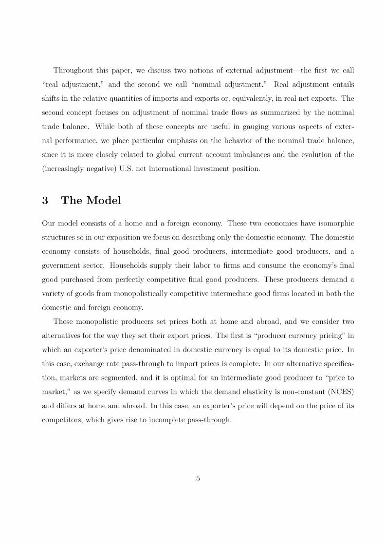
In our other alternative, we assume that markets are segmented, allowing a firm to price
to market (PTM). In this case, a firm sets its export price to maximize profits in its foreign
market:
max (etP∗mt(i)−MCt) M∗
t (i), (12)
taking marginal cost and its demand curve, M∗t (i), as given. Profit maximization implies that
the monopolist chooses to set its price as a markup over marginal cost:
P ∗mt(i) = µ∗mt(i)
MCt
et
. (13)
In the above, a home exporter’s markup, µ∗mt(i) is given by:
µ∗mt(i) =
[1− 1
|ε∗mt(i)|]−1
,
where |ε∗mt(i)| is (the absolute value of) the demand elasticity:
ε∗mt(i) =1
1− γ
[1 + η
(P ∗
mt(i)
P ∗mt
) 11−γ
(P ∗
mt
Γ∗t
) ρρ−γ
]−1
. (14)
According to equations (13) and (14), a firm’s pricing decision depends not only on its marginal
cost (denominated in foreign currency) but also on Γ∗t , the prices of its competitors in the foreign
market. We calibrate our demand aggregator to allow for strategic complementarity in price
setting.11 In that case, |ε∗mt(i)| is an increasing function ofP ∗mt
Γ∗tand a firm’s desired markup
will be a decreasing function of this relative price. As a consequence, a domestic exporter
will find it desirable to lower its markup in response to a shock that raises its costs relative
to its competitors, because the exporter does not want its price to deviate too far from its
11 We follow Woodford (2003) and define pricing decisions to be strategic complements if an increase in theprices charged for other goods increases a firm’s own optimal price.
9

competitors’ prices. In this way, pass-through of exchange-rate changes to import prices can
be incomplete even in the absence of nominal price rigidities.
In the PTM alternative, a firm chooses contingency plans for domestic prices to maximize
its expected discounted stream of profits from the domestic market:
Et
∞∑j=0
ψt,t+j [Pdt+j(i)−MCt+j] Adt+j(i) [1− φdt+j(i)] , (15)
taking marginal cost, its stochastic discount factor, ψt,t+1, and the demand schedule for its good
as given.12 In the PCP alternative, a firm has a similar objective function except that now it
takes into account that its price influences demand both at home and abroad:
Et
∞∑j=0
ψt,t+j [Pdt+j(i)−MCt+j] (Adt+j(i) + Mt+j(i)) [1− φdt+j(i)] . (16)
As noted earlier, our calibrated demand curves imply a strategic complementarity in price set-
ting, and, as in Kimball (1995) and Dotsey and King (2005), will be associated with more
nominal domestic price inertia and output persistence than sticky price models with CES de-
mand curves. This greater nominal domestic price inertia will be true regardless of whether
export prices are determined according to PCP or PTM.
3.3 Households
The utility function of the representative household in the home country is
Et
∞∑j=0
βjlog(Ct+j − κCA
t+j−1
)− χ0
L1+χt+j
1 + χ, (17)
where the discount factor β satisfies 0 < β < 1 and Et is the expectation operator conditional on
information available at time t. As in Smets and Wouters (2003), we allow for the possibility of
external habits, where a household cares about its consumption, Ct, relative to lagged aggregate
consumption, CAt−1. The period utility function also depends on labor hours, Lt.
12 For convenience, we have suppressed all of the state indices. In the household problem, we define ξt,t+1
to be the price in period t of a claim that pays one unit of the home currency if the specified state occurs inperiod t + 1. The corresponding element of ψt,t+1 equals ξt,t+1 divided by the probability that the specifiedstate occurs.
10

A household faces a flow budget constraint in period t which states that its expenditures
and net accumulation of financial assets must equal its disposable income:
PtCt+PtIt+
∫
s
ξt,t+1BDt+1−BDt+etP
∗BtBFt+1
φbt
−etBFt = WtLt+RKtKt+Ωt−Tt−PtφIt. (18)
A household’s disposable income consists of its labor income (WtLt), income from renting capital
to firms (RKtKt), and an aliquot share of the profits of the domestic firms (Ωt). Households
also pay lump-sum taxes (Tt) and purchase the final good for investment (It). A household’s
investment augments capital according to:
Kt+1 = (1− δ)Kt + It. (19)
As in Christiano, Eichenbaum, and Evans (2005), households also pay a cost to changing the
level of gross investment from the previous period:
φIt =φI
2
(It − It−1)2
It−1
. (20)
We assume that a household can engage in frictionless trading of a complete set of contingent
claims with other domestic households. We denote ξt,t+1 as the price of an asset that pays one
unit of domestic currency in a particular state of nature at date t + 1, while BDt+1 represents
the quantity of such claims purchased by a household at time t.
While asset markets are complete within a country, we assume that trade in international
assets is restricted to a non-state contingent nominal bond. Accordingly, in equation (18),
BFt+1 represents the quantity of a non-state contingent asset purchased at time t that pays
one unit of foreign currency in the subsequent period, and P ∗Bt is the foreign currency price of
the bond. We follow Turnovsky (1985) and assume there is an intermediation cost φbt paid by
households in the home country for purchases of foreign bonds, which is necessary to ensure
that the model has a unique steady state.13 More specifically, the intermediation costs depend
on the ratio of economy-wide holdings of net foreign assets to nominal output and are given by:
φbt = exp
[−φb
(etB
AFt+1
PY tYt
)+ νbt
]. (21)
13 This intermediation cost is asymmetric, as foreign households do not face these costs. Rather, they collectprofits on the monopoly rents associated with these intermediation costs. As discussed in Schmitt-Grohe andUribe (2003), this way of closing the model delivers similar dynamics to other alternative approaches.
11

In the above, νbt is a mean-zero stochastic process, which we interpret as a risk-premium shock
or a shock to the uncovered interest-rate parity condition. Abstracting from this shock, if the
home economy in aggregate is a net lender, then a household will earn a lower return on any
holdings of foreign bonds. By contrast, if the economy is a net debtor, a household will pay a
higher return on any foreign debt.
While it is difficult to give the risk premium shock a structural interpretation, we see it as the
nearest equivalent in general equilibrium to the partial equilibrium case in which the exchange
rate is exogenous. As such, we use the risk premium shock as an illustrative device for comparing
our partial and general equilibrium results. We then characterize how the transmission of other
shocks on the trade balance is affected by incomplete pass-through.
In every period t, a household maximizes the utility functional (17) with respect to con-
sumption, investment, the end-of-period capital stock, labor, holdings of domestic contingent
claims, and holdings of the international asset subject to its budget constraint (18) and the
evolution of capital (19). In doing so, a household takes as given prices and aggregate quantities
such as lagged aggregate consumption and the aggregate net foreign asset position.
3.4 The Government and Monetary Policy
Some of the final good is purchased by the government so that At can be interpreted as total
absorption:
At = Ct + It + Gt. (22)
We assume that government purchases (Gt) follow an exogenous, stochastic process and do not
directly affect the utility function of the representative household. The government’s budget is
balanced every period which implies that lump-sum taxes are equal to government purchases.
We assume that monetary policy follows an interest rate rule:
it = γππt + γyyt + εmt, (23)
where the symbol ‘ ˆ ’ denotes the logarithmic deviation of a variable from its steady state
value. Hence, it denotes the (gross) quarterly nominal interest rate expressed as a log-deviation
12

from steady state, and πt = Pdt
Pdt−1is the quarterly rate of inflation. The interest rate rule also
includes the log deviation of output from potential output, where potential output is defined
as the domestic economy’s level of output in the absence of sticky domestic prices. Finally, εmt
is a stochastic disturbance which can be interpreted as a monetary policy shock.
4 Partial Equilibrium Analysis
To gain intuition for the relationship between exchange rate pass-through and the trade balance,
we first consider a simple partial-equilibrium version of our model. In this partial equilibrium
framework, we consider only the PTM case and focus on a symmetric equilibrium in which all
intermediate good producers choose the same price (i.e., P ∗mt(i) = P ∗
mt ∀i). Expressing variables
in real terms, the log-linearized version of a home exporter’s pricing decision in the PTM case
(equation 13) can be written as:
p∗mt = βx (mct − qt) , (24)
where qt =etP ∗tPt
is the real exchange rate, p∗mt = P ∗mt− P ∗
t is the foreign import price relative to
the price of the final good, and mct = MCt−Pt denotes the deviation of real marginal cost from
its steady state value. In equation (24), βx determines the responsiveness of a firm’s relative
export price to real marginal cost denominated in foreign currency.14 With βx < 1, a home
exporter finds it optimal to adjust its price in response to the prices of its competitors and will
not fully pass through changes in marginal costs because of the competitive disadvantage that it
implies. Since a foreign exporter behaves in an identical manner, there is a similar relationship
for the price of a good imported to the home country:
pmt = βm (mc∗t + qt) . (25)
14 To derive equation (24), we have also used the fact that Γ∗t = P ∗t . Also, we can show that βx =1
1−ηµm( ρ(γ−1)γ−ρ )
, where the steady state markup is given by µm = 1γ+η(γ−1) . In this derivation, we have used
the fact that in the non-stochastic steady state all relative prices are equal to one, as the two economies aresymmetric.
13

It is also convenient to rewrite equation (24) defining the export price in domestic currency
units (i.e., pxt = qt + p∗mt):
pxt = βxmct + (1− βx)qt. (26)
While a change in the exchange rate can affect a firm’s pricing behavior indirectly by affect-
ing real marginal cost in domestic currency, we abstract from this general equilibrium effect.
We, thus, compute the direct effect by holding mct constant and partially differentiating the
prices in equations (26) and (25) with respect to the real exchange rate:
∂pxt
∂qt
= 1− βx and∂pmt
∂qt
= βm. (27)
According to equation (27), a one percent depreciation of the home currency (i.e., an increase
in qt) leads to an increase in the import price paid by a home household of βm and an increase
in a home firm’s export price of 1 − βx. (The corresponding import price paid by a foreign
household falls by βx). Thus, we equate βm with pass-through to the import price and 1− βx
with pass-through of the exchange rate to the export price.
With “direct” or partial equilibrium pass-through defined in this way, we now turn to
examining the implications of various values of βx and βm for trade adjustment. In a symmetric
equilibrium, we can rewrite equation (5) to express aggregate import demand as:
Mt =ω
1 + ω
[1
1 + η
(Pmt
Γt
) ργ−ρ
+η
1 + η
]At. (28)
Log-linearizing this equation, we have:
Mt = −αmpmt + At, (29)
where αm = ρρ−γ
11+η
> 0 is the elasticity of aggregate imports (Mt) with respect to its relative
price. We can also derive a similar condition for foreign import demand or home export demand:
Xt = M∗t = −αx (pxt − qt) + A∗
t , (30)
where αx > 0 is the elasticity of a aggregate home exports with respect to its relative price.
14

The response of real exports and imports to an exchange rate change depends crucially on
the values of βx and βm. This importance can be seen by partially differentiating Mt and Xt
with respect to the exchange rate, holding At and A∗t constant:
∂Mt
∂qt
= −αm∂pmt
∂qt
= −αmβm and∂Xt
∂qt
= −αx
(∂pxt
∂qt
− 1
)= αxβx. (31)
According to (31), a one percent real depreciation of the home currency induces a larger decrease
in real imports when import price pass-through is high. Similarly, the depreciation leads to a
larger increase in exports when the export price is insensitive to the exchange rate (i.e., βx = 1
so that import price pass-through in the foreign country is complete). Thus, adjustment of
real trade volumes in response to an exchange rate change will be larger when pass-through to
import prices in both countries is complete.
To examine the relationship between pass-through and the nominal trade balance, it is
convenient to define the ratio of nominal exports to imports, τt = PxtXt
PmtMt. Expressing this ratio
as a log-deviation from steady state:
τt = pxt − pmt + Xt − Mt, (32)
it is clear that nominal adjustment depends on the responses of the terms of trade, Pxt
Pmt, and
real net exports, Xt
Mt. Using expressions (27) and (31), the partial effect of an exchange rate
change on τt is given by:
∂τt
∂qt
=
(∂pxt
∂qt
− ∂pmt
∂qt
)+
∂Xt
∂qt
− ∂Mt
∂qt
= (1− βx − βm) + αxβx + αmβm. (33)
The first term in the parentheses is the effect of an exchange rate change on the terms of trade,
and the other two terms are the effects of the exchange rate change on real trade volumes. If the
trade-price elasticities are equal to unity (i.e., αx = αm = 1), then nominal adjustment is inde-
pendent of the pass-through assumptions, and the nominal trade balance will increase by one
percent of the value of exports in response to a one percent depreciation of the home currency.
In this case, nominal adjustment is independent of pass-through, because in both the home
15

and foreign country nominal expenditures on imports are unchanged, as movements in domes-
tic currency prices are offset by proportionate shifts in real imports. The home trade balance
improves in response to a depreciation of the home currency, however, because the unchanged
foreign expenditure on imports translates into increased home-currency export receipts.
Although in partial equilibrium the response of the trade balance is independent of the pass-
through assumptions when αx = αm = 1, the forces that bring about trade balance adjustment
are different in a low and high pass-through environment. In a high pass-through environment
(i.e., βx + βm > 1), the nominal trade balance rises in response to a depreciation, as real net
exports increase enough to offset a fall in the terms of trade. By contrast, in a low pass-through
environment (i.e., 0 ≤ βx + βm < 1), the terms of trade increase in response to a depreciation,
and both the rise in the terms of trade and higher real net exports contribute to an increase in
the trade balance.
If αx, αm > 1, then higher values of βx and βm induce greater trade balance adjustment.
With αm > 1, both real and nominal imports fall in response to a depreciation. Because
this decline is greater for higher values of βm, a higher value of βm is associated with more
trade balance adjustment. Similarly, with αx > 1, real and nominal exports rise following a
depreciation, and this increase is larger for higher values of βx.
It is also interesting to note that the usual Marshall-Lerner condition needs to be modified
in an environment with incomplete pass-through. This condition states that for a depreciation
of the domestic currency to lead to a rise in the trade balance, the sum of the export and import
price elasticities must be greater than one (i.e., αx+αm > 1). However, this condition is derived
assuming complete pass-through. From equation (33), we can see that for a depreciation to
induce an improvement in the trade balance, it must be true that:
αxβx + αmβm > βx + βm − 1. (34)
In the complete pass-through environment (βx = βm = 1), this condition is the same as the
usual Marshall-Lerner condition. More generally, this modified version of the Marshall-Lerner
condition states that for a depreciation of the domestic currency to lead to an increase in the
trade balance, its stimulative effects on real exports and real imports must be greater than its
16

effect on the terms of trade. Notably, if βx, βm ≤ 12, then equation (34) is satisfied for any
positive values of the trade price elasticities.
5 General Equilibrium Analysis
5.1 Three Benchmark Scenarios
Our partial equilibrium framework assumed that the exchange rate was exogenous and held
variables such as home and domestic absorption constant. We now relax these assumptions
by simulating the effects of various shocks in our general equilibrium model. For each of the
shocks that we study, we consider three scenarios:
• Scenario 1: High import price pass-through in the home country and in the foreigncountry. In this case, both domestic exporters and foreign exporters practice producercurrency pricing.
• Scenario 2: Low import price pass-through in the home and foreign countries. In thisinstance, domestic and foreign exporters both engage in pricing to market.
• Scenario 3: Low import price pass-through in the home country and high import pricepass-through in the foreign country. In this scenario, the home country and the foreigncountry are no longer symmetric. Domestic exporters engage in producer currency pricing,while foreign exporters practice pricing to market. This scenario is consistent with a worldin which trade prices are set in the home country and are translated abroad by movementsin the exchange rate.
While all three of these scenarios are useful conceptual benchmarks, it is helpful to make a
few comments about their empirical relevance for the United States. The evidence discussed
above indicates that pass-through to U.S. import prices is now relatively low, which differs
significantly from the features of Scenario 1. As noted above, the results for others countries
are somewhat less conclusive. The evidence suggests that import price pass-through for some
major countries (e.g., Japan and Germany) is also low; but for some smaller countries (e.g.,
Australia and Sweden), pass-through to import prices appears to have remained high. As such,
the global economy at present appears to have features of both Scenario 2 and Scenario 3.
17

5.2 Model Calibration
We solve our general equilibrium model by log-linearizing the equations around the steady
state. To obtain the reduced-form solution of the model, we use the numerical algorithm of
Anderson and Moore (1985), which provides an efficient implementation of the method proposed
by Blanchard and Kahn (1980).
For simplicity, we choose the model parameters to be the same across the two economies.
Also, we calibrate the model at a quarterly frequency by setting β = (1.03)−0.25 and δ = 0.025.
The utility function parameter χ is set to 1.5, which implies a Frisch labor supply elasticity of
23, while χ0 is chosen so that the steady state level of hours worked is normalized to unity. We
set the degree of habit persistence in consumption, κ, equal to 0.8, and the cost of adjusting
investment, φI , equal to 4, a value in line with the estimate of Christiano, Eichenbaum, and
Evans (2005). We choose a small value for the financial intermediation cost, φb = 0.0001, which
is necessary to ensure that net foreign assets are stationary.
The Cobb-Douglas production function parameter, α, equals 0.36, which implies a steady
state (quarterly) capital to output ratio of around 9. The steady state investment to output
ratio is 23 percent, while government consumption is 16 percent of steady state output. We
choose ω so that the steady state import to output ratio is 12.5 percent. Given that trade is
balanced in steady state, the export share in both economies is also 12.5 percent.
For the demand curves, we set γ = 1.03, ρ = 0.885, and η = −7. These values imply a steady
state markup over marginal cost of 22 percent and a price elasticity of aggregate trade flows of
unity. In addition, in the case in which both home and foreign exporters price to market, they
imply that exchange rate pass-through to import prices is about 40 percent. Using data for the
past couple of decades, this value is in line with empirical estimates for the United States, but
somewhat above estimates obtained from data over only the past ten to fifteen years.
We set the adjustment cost parameter for domestic prices, φd, to be consistent with four-
quarter contracts. For the monetary policy rule, we follow Taylor (1993) and set γπ = 1.5 and
γy = 0.54
.
18

5.3 A 10 percent Depreciation of the Home Currency
We first consider a shock that raises the risk premium on home assets. The shock is assumed
to be persistent with an AR(1) coefficient of 0.98, so that its effects die out slowly over time.
As shown in the upper-left panel of Figure 1, the shock is scaled to deliver a 10 percent
initial depreciation of the real exchange rate. (In the figure, an upward movement indicates a
depreciation.) Given the differing extent of pass-through in the three scenarios, risk premium
shocks of varying magnitudes are required to deliver the same initial 10 percent depreciation.
This scaling of the risk premium shock allows us to isolate the additional effect on the trade
balance arising from changes in home and foreign absorption relative to the partial equilibrium
results. Later, we explicitly take into account the endogeneity of the exchange rate and examine
how its response varies across the three scenarios.
When import price pass-through at home and abroad is high (Scenario 1), home consumer
prices post comparatively large initial rises, and home output moves well above potential. This
elicits a relatively aggressive monetary policy response and results in a higher real interest rate
than in the other two cases. This rise in the real interest rate, in turn, causes the real exchange
rate to begin to retrace its initial decline and brings the output gap back toward baseline, as
the compression of domestic demand offsets a rise in net exports. In the other two scenarios,
where import price pass-through in the home country is low, the effects are generally similar
but smaller in magnitude.
We turn now to the behavior of the external sector. As shown in the upper-left panel of
Figure 2, when home import price pass-through is high (Scenario 1), the import price relative
to the consumer price level jumps up, closely tracking the exchange rate as foreign exporters
maintain the price in their domestic currencies.15 For the other two scenarios, moves in the
relative import price are more subdued, consistent with the lower pass-through. As seen in the
upper-right panel, real imports fall sharply in the high pass-through case partly in response
to the rise in relative import prices, while real imports decline more moderately in the two
15 Throughout this paper we consider the behavior of trade prices relative to the price of domestic and foreignconsumer goods. We do this to abstract from trends in absolute price levels (arising from monetary policyactions), which cloud the analysis and are not material to the interpretation of our results.
19
scenarios in which pass-through is low.
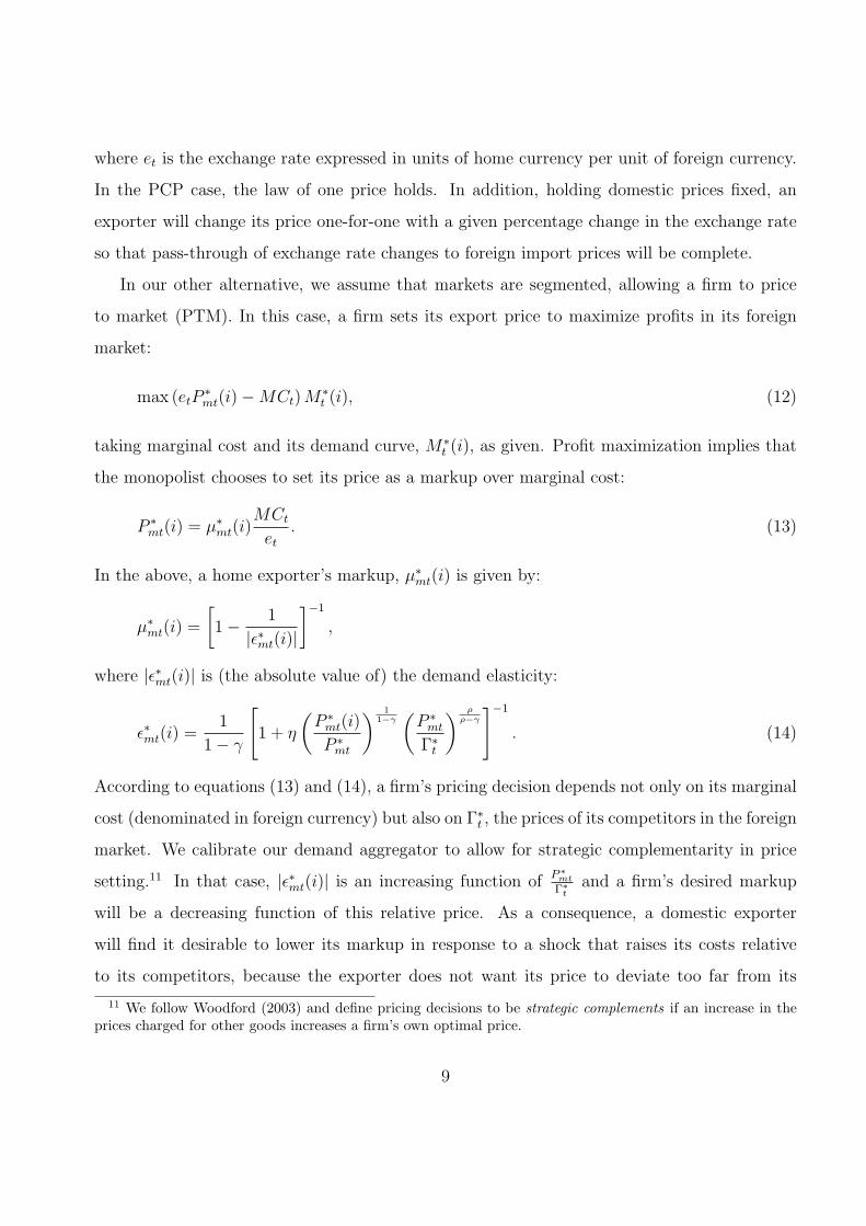
The lower-left panel shows that nominal imports fall in all three scenarios, as the declines
in import quantities more than offset rises in import prices. The decline in nominal imports is
largest when pass-through is high in both countries and smallest when pass-through is low in
both countries. As noted above, in partial equilibrium and with unitary import-price elasticities,
nominal expenditure on imports is unaffected by a move in the exchange rate. Thus, the decline
in nominal imports relative to baseline in all three scenarios is driven by general-equilibrium
feedback effects, as tighter monetary policy slows domestic absorption, which—in turn—weighs
on real and nominal imports. These feedback effects are most pronounced when pass-through
is high or, equivalently, when domestic prices and output are most sensitive to the exchange
rate.
We now examine the behavior of the home country’s exports. High import price pass-
through in the foreign market means that exporters maintain their domestic-currency prices in
the face of exchange rate changes. Accordingly, as shown in the upper-left panel of Figure 3,
there is comparatively little movement in the price of exports relative to consumption goods
in the two cases in which import price pass-through in the foreign market is high (Scenarios 1
and 3). In contrast, when import price pass-through in the foreign market is low (Scenario 2),
the home currency price of exports moves up markedly. As shown in the upper-right panel, in
the cases with high foreign import price pass-through, the export price—expressed in terms of
foreign currency (or, equivalently, the foreign import price)—falls significantly; and, as seen in
the lower left-panel, the quantity of home exports rises correspondingly. When pass-through in
the foreign market is low, the price in terms of foreign currency falls more modestly, and the
volume of home exports consequently rises only a little.
The bottom-right panel shows the behavior of the home country’s nominal exports. In all
three scenarios, we see a marked rise in nominal exports, but the impetus for the rise differs
significantly with pass-through. In the low pass-through case, Scenario 2, quantities move
relatively little, but domestic-currency prices step up with the exchange rate. In the other two
cases, the export price in domestic-currency terms is little changed, but quantities rise briskly.
20

As noted above, in partial equilibrium, the home country’s export earnings rise propor-
tionately with the fall in the exchange rate; thus, a one percent depreciation of the exchange
rate raises home export revenues by one percent. In these simulations, nominal exports move
more than one-for-one with the exchange rate, indicating that additional general equilibrium
effects are at work. Most important, an easing of monetary policy abroad, in response to the
appreciation of the foreign currency, stimulates foreign demand and consequently raises the
home country’s exports. This effect is largest in Scenarios 1 and 3—when foreign import price
pass-through is high and, as a result, when the monetary policy response abroad is relatively
aggressive.
We now look at several measures of the home country’s external balance to assess the
bottom-line impact on external adjustment. First, to assess the implications for real trade
volumes, we consider the evolution of the ratio of real exports to real imports, which we call
the “real trade balance.” As shown in the upper-left panel of Figure 4, when import price
pass-through is low in both countries, adjustment in the real trade balance is relatively muted.
In contrast, real adjustment is most significant when import price pass-through is high in both
countries—in this case we see a significant rise in real exports and a significant drop in real
imports. The case in which import price pass-through is low at home but high abroad is between
the two others, reflecting a large response from real exports but a smaller response from real
imports.
We take the ratio of nominal exports to nominal imports as our measure of the nominal trade
balance. As displayed in the upper-right panel, the results here are much more similar across
the three scenarios than is the case for the real trade balance; shifts in the terms of trade (i.e.,
export prices relative to import prices) tend to offset the effects of real adjustment. Specifically,
as shown in the lower-left panel, when import price pass-through is high in both countries, the
domestic country’s terms of trade decline significantly as import prices rise relative to export
prices. In the case in which pass-through is low in both countries, export prices rise a little more
than import prices, and the terms of trade improve slightly. The results for the asymmetric
case lie between the other two cases.
21
Thus, the nominal trade balance improves in all three scenarios. In the high pass-through
world, adjustment occurs as large declines in real imports and increases in real exports are offset
by a significant deterioration in the terms of trade. When import price pass-through at home
and abroad is low, quantities move by less, but the terms of trade make a positive contribution
to the improvement in the nominal trade balance. In the asymmetric case, adjustment is driven
mainly by a surge in export quantities. The results for the trade balance as a share of GDP
(the lower-right panel) are broadly similar to those for the ratio of nominal exports to nominal
imports.
In partial equilibrium, the response of the nominal trade balance to changes in exchange
rates is the same regardless of the degree of exchange rate pass-through, given our maintained
assumptions. Thus, the fact that the three scenarios manifest varying degrees of improvement
in the nominal trade balance reflects the differing general equilibrium effects on activity and
absorption under differing pass-through assumptions.
5.4 An Identical Shock to the Risk Premium
Building on the results from the first simulation, our second simulation introduces another
important general equilibrium effect. Specifically, the previous simulation modulated the risk-
premium shock in the three scenarios to deliver an initial 10 percent depreciation of the exchange
rate. In contrast, this second simulation considers a shock to the risk premium on home assets
that is identical in each of the three scenarios. As shown in the upper-left panel of Figure 5,
this shock causes the exchange rate to depreciate by somewhat less than 10 percent in Scenario
1 (when import price pass-through at home and abroad is high), by somewhat more than 10
percent in Scenario 2 (when import price pass-through at home and abroad is low), and by
exactly 10 percent in Scenario 3 (when import price pass-through is low at home but high
abroad).
These contrasting outcomes reflect the fact that the underlying structure of the home and
foreign economies differs across the three scenarios. As we have shown in the previous simu-
lation, with higher pass-through, the depreciation of the home currency puts greater upward
22
pressure on domestic prices and output and, accordingly, leads to larger rises in domestic inter-
est rates. This more aggressive tightening of monetary policy when pass-through is high also
serves to limit the initial depreciation of the exchange rate.16 By symmetric logic, the upfront
depreciation of the exchange rate is relatively large when pass-through is low.
In comparing the results of this simulation and the previous simulation, a useful observation
is that by construction the exchange rate depreciates the same amount in Scenario 3 in both
simulations. As such, results for this scenario are identical to their counterparts in the previous
figures. With this observation in hand, it becomes clear that the pattern of responses of the real
interest rate and absorption in this simulation is generally consistent with that in the previous
simulation. That said, the magnitude of the responses across the scenarios is more similar in
this simulation, as there are smaller moves in the high-pass through case than in the previous
simulation and larger moves in the low pass-through case. This reflects that in the high pass-
through scenario the initial depreciation is more muted than in the previous simulation, while
in the low pass-through scenario the depreciation is larger.
As shown in the top-right panel, we continue to see greater adjustment of the real trade
balance in the high pass-through case, but these results are also more similar across the three
scenarios than was the case in the first simulation. Specifically, for the high pass-through case,
the smaller depreciation of the exchange rate and the smaller decline in absorption translate
into a smaller decline in real imports; similarly, with less support from the exchange rate—
and with foreign demand also less supportive—real exports rise by less than in the previous
simulation. The results for the low pass-through case are symmetric. As in the previous
simulation, however, differences in the performance of the real trade balance are partially offset
by moves in the terms of trade—most notably for the high pass-through case.
The bottom-right panel shows the implications for the nominal trade balance. The striking
result is that the path of the trade balance across the three scenarios is quite similar, at
least after the first few quarters. This suggests that the additional general equilibrium effect
considered in this simulation—the fact that a given risk premium shock results in a larger move
16 By the same token, when pass-through abroad is high, interest rates there fall by more, which further limitsthe upfront depreciation of the domestic currency.
23

in the exchange rate when pass-through is low—roughly offsets the effects operating through
absorption that were highlighted in the first simulation. More generally, under our benchmark
calibration, we find that the adjustment of the nominal trade balance in response to a similar-
sized risk premium shock does not vary systematically with pass-through. This conclusion is
similar in spirit to our partial equilibrium results discussed above.
Notably, however, the results of this simulation are still quite consistent with the bottom-
line implications of the first simulation: When pass-through is low, the exchange rate must
depreciate more to deliver a given amount of nominal adjustment. The key insight here is that
the additional exchange rate depreciation that is required arises as an endogenous response to
moves in interest rates. A risk premium shock elicits less tightening of monetary policy with
low pass-through and, as such, the currency depreciates more when pass-through is low.
5.5 Other Types of Shocks
So far, we have illustrated how the extent of exchange rate pass-through affects trade adjust-
ment using shocks to the risk premium. Since it is difficult to give these shocks a structural
interpretation, we now demonstrate that our results are applicable across a broad set of shocks.
Accordingly, Table 1 displays results for a contraction in government spending, a monetary
expansion, and an improvement in technology, and (for the sake of comparison) a risk premium
shock. In each case, the trade price elasticities are assumed to be near unity, and the shocks
are scaled such that the exchange rate depreciates 1 percent in the low pass-through scenario
after eight quarters.
The results of these additional simulations broadly confirm the conclusions reported above.
The following features are particularly notable. First, for reasons highlighted in the previous
section, the exchange rate depreciates less in the high pass-through scenario than in the low
pass-through scenario for all four types of shocks. Second, the moves in absorption in the high
pass-through case are systematically less supportive of imports (i.e., the change in absorption
is either less positive or more negative) than in the low pass-through case, as monetary policy
consistently tightens more when pass-through is high. Third, for each shock, the change in the
24

real trade balance in the high pass-through case is either more positive or less negative than in
the low pass-through case. This reflects the fact that absorption is less supportive of imports in
the high pass-through case; in addition, although the exchange rate depreciates less in the high
pass-through case, real variables (including imports and exports) are more sensitive to a given
move in the exchange rate when pass-through is high. Fourth, as in the two simulations above,
the terms of trade deteriorate markedly in the high pass-through case but improve, although
typically only slightly, in the low pass-through case. Finally, with moves in the terms of trade
offsetting differing moves in the real trade balance, we again find that the impact on the nominal
trade balance is quite similar in the high pass-through and low pass-through scenarios.
5.6 Sensitivity Analysis
In our previous simulations, we have shown that the nominal trade balance is less sensitive to
a given move in the exchange rate when pass-through is low. However, low pass-through also
means that the exchange rate tends to move more in response to a given shock. The relative
importance of these offsetting effects depends on the structural features of the economy. To
explore this observation further, we now consider two alternative calibrations of our model. In
the first, the trade price elasticities are greater than unity. In the second, absorption moves
relatively sluggishly. In each case, we compare the results to those reported in our second
simulation (Section 5.4).
5.6.1 Higher Trade Price Elasticities
We also consider an alternative in which the trade price elasticities are set equal to three. These
values were chosen to be consistent with our reading of literature suggesting that trade price
elasticities estimated using disaggregated data are typically higher than those based on macro
data. The risk premium shock that we use here is identical to that in the second simulation,
but—as displayed in the top-left panel of Figure 6—the exchange rate now responds much less
in all three scenarios. This result reflects the fact that with the larger trade price elasticities,
volumes of imports and exports and, hence, real net exports are more sensitive to moves in
25

the exchange rate. This induces a more sustained tightening of monetary policy than was
seen in the previous simulation. (The initial moves in monetary policy are not significantly
different than before, but the real interest rate stays above baseline more persistently.) The
more sustained response of monetary policy also means that absorption stays below baseline
somewhat more persistently.
As shown in the top-right panel, the real trade balance in all three cases rises much more
significantly in this simulation than in the second simulation. This reflects that import and
export demand are now more sensitive to the risk premium shock, as the effects of the higher
trade price elasticities more than offset the fact that the dollar depreciates by less; in addition,
the somewhat longer-lived decline in absorption weighs on real imports. In contrast, given the
more muted response of the real exchange rate, shifts in trade prices and, thus, in the terms of
trade are more muted than in the second simulation. As such, shifts in the terms of trade are
now insufficient to offset the moves in real trade quantities, which have been magnified by the
higher trade price elasticities. Consequently, the extent of pass-through now affects the degree
of nominal adjustment—with the trade balance as a share of GDP (the bottom-right panel)
rising significantly more in the high pass-through case than in the low pass-through case. It
is also noteworthy that in each scenario, the responsiveness of the nominal trade balance is
more pronounced than before, as the higher trade price elasticities and the higher resulting
sensitivity of real trade volumes to the exchange rate lifts the nominal trade balance.
5.6.2 Greater Habit Persistence and Investment Adjustment Costs
In this section, we consider a scenario in which absorption in both the home and foreign
economies responds more sluggishly to shocks than in the previous simulations. This is achieved
by increasing the habit persistence parameter (κ) from 0.8 to 0.95, and the cost of adjusting
investment (φI) from 4 to 15. The shock is the same as in the second simulation, and the trade
price elasticities are set equal to one. With this parameterization of the model, we find that
the nominal trade balance actually moves more in the low pass-through case.
The results of this simulation are reported in Figure 7. Compared with the second simula-
26
tion, the increased sluggishness of private spending abroad means that domestic exports—and,
hence, the domestic output gap—respond relatively slowly. The upfront contraction in ab-
sorption is also less pronounced, reflecting the greater degree of habit persistence and cost of
adjusting investment. As shown in the upper-right panel, the real trade balance consequently
moves less in each scenario than was the case in the second simulation, with the response in the
high pass-through case being particularly compressed. In contrast, the moves in the terms of
trade are similar to those in Figure 5, reflecting the comparable pattern and magnitude of ex-
change rate changes. The net result is that the nominal trade balance improves more in the low
pass-through case, as the reaction of the terms of trade now more than offsets the compressed
response of the real trade balance. The intuition for this result is that in the second and third
scenarios low pass-through already constrains the response of the real economy. As such, the
incremental effects of more sluggish absorption are felt most strongly in the high pass-through
environment.
6 Conclusion
In this paper, we have developed an open economy DGE model in which firms optimally choose
to vary their markups, allowing pass-through to be incomplete. We have used this model to
study the relationship between exchange rate pass-through and external adjustment.
One notable result that has emerged from our work is that real economic variables—
including absorption and real exports and imports—tend to respond less to a given-sized shock
when pass-through is low. This reflects the fact that with low pass-through foreign exporters
absorb a portion of the shock into their margins. As a result, domestic inflation is less sensi-
tive to moves in the exchange rate, and the required shift in the stance of monetary policy is
correspondingly less pronounced. These features of the low pass-through world tend to limit
adjustment of the nominal trade balance, holding all else equal. But the fact that monetary
policy moves less when pass-through is low gives rise to another important effect, which has
offsetting implications for the nominal trade balance. That is, the exchange rate tends to move
27

more in response to a given-sized shock.
A complementary perspective on our results is that a given quantum of improvement in the
nominal trade balance requires a larger move in the real exchange rate when pass-through is
low. A key insight of our work, however, is that much (or all) of the additional exchange rate
depreciation that is required arises as an endogenous response to moves in interest rates. The
exchange rate moves more in the low pass-through world, but—as real economic variables are
less sensitive to moves in the exchange rate—the broader economic implications of these larger
exchange rate moves are limited.
28

References
Adolfson, M. (2004). Exchange Rate Pass-through—Theory, Concepts, Beliefs and SomeEvidence. Sveriges Riksbank, mimeo.
Anderson, G. and G. Moore (1985). A Linear Algebraic Procedure for Solving Linear PerfectForesight Models. Economic Letters 17, 247–52.
Armington, P. (1969). A Theory of Demand for Products Distinguished by Place of Produc-tion. IMF Staff Papers 16, 159–176.
Bergin, P. and R. Feenstra (2001). Pricing-to-Market, Staggered Contracts, and Real Ex-change Rate Persistence. Journal of International Economics 54, 333–59.
BIS (2005). 75th Annual Report. Basel, Switzerland: Bank for International Settlements.
Blanchard, O. and C. Kahn (1980). The Solution of Linear Difference Models under RationalExpectations. Econometrica 48, 1305–1311.
Campa, J. and L. Goldberg (2005). Exchange Rate Pass-Through into Import Prices. Reviewof Economics and Statistics 87, 679–690.
Christiano, L., M. Eichenbaum, and C. Evans (2005). Nominal Rigidities and the DynamicEffects of a Shock to Monetary Policy. Journal of Political Economy 113, 1–45.
Corsetti, G. and P. Pesenti (2005). International Dimensions of Optimal Monetary Policy.Journal of Monetary Economics 52, 281–305.
Devereux, M. and C. Engel (2002). Exchange Rate Pass-Through, Exchange Rate Volatility,and Exchange Rate Disconnect. Journal of Monetary Economics 49, 913–940.
Devereux, M. and C. Engel (2003). Monetary Policy in the Open Economy Revisited: PriceSetting and Exchange Rate Flexibility. Review of Economic Studies 70, 765–783.
Dotsey, M. and R. King (2005). Implications of State-Dependent Pricing for DynamicMacroeconomic Models. Journal of Monetary Economics 52, 213–42.
Ellis, L. (2004). Exchange Rates and Monetary Policy: the Australian Context. Reserve Bankof Australia, mimeo.
Frankel, J., D. Parsley, and S. Wei (2005). Slow Pass-through around the World: A NewImport for Developing Countries? NBER Working Paper 11199.
Goldberg, P. and M. Knetter (1997). Goods Prices and Exchange Rates: What Have WeLearned? Journal of Economic Literature 35, 1243–72.
Gust, C., S. Leduc, and R. Vigfusson (2006). Trade Integration, Competition, and the De-cline in Exchange Rate Pass-through. Board of Governors of the Federal Reserve SystemInternational Finance Discussion Papers 864.
Heath, A., I. Roberts, and T. Bulman (2004). Inflation in Australia: Measurement andModelling. In C. Kent and S. Guttmann (Eds.), The Future of Inflation Targeting, pp.167–207. Reserve Bank of Australia, Sydney.
29

Hooper, P. and J. Marquez (1995). Exchange Rates, Prices, and External Adjustment in theUnited States and Japan. In P. Kenen (Ed.), Understanding Independence, pp. 107–168.Princeton, NJ: Princeton University Press.
Ihrig, J., M. Marazzi, and A. Rothenberg (2006). Exchange-Rate Pass-Through in the G-7 Countries. Board of Governors of the Federal Reserve System International FinanceDiscussion Papers 851.
IMF (2005). United States: Selected Issues. Washington, D.C.: International Monetary Fund.
Kimball, M. (1995). The Quantitative Analytics of the Neomonetarist Model. Journal ofMoney, Credit, and Banking 27, 1241–77.
Marazzi, M., N. Sheets, and R. Vigfusson (2005). Exchange Rate Pass-Through to U.S.Import Prices: Some New Evidence. Board of Governors of the Federal Reserve SystemInternational Finance Discussion Papers 833.
Marquez, J. (2002). Estimating Trade Elasticities. Dordrecht, The Netherlands: Kluwer Aca-demic Publishers.
McDaniel, C. and E. Balistreri (2003). A Review of Armington Trade Substitution Elastici-ties. Integration and Trade 7, 161–173.
Nessen, M. (2004). Exchange Rate Pass-through, Inflation, and Monetary Policy. SverigesRiksbank, mimeo.
Rotemberg, J. (1982). Sticky Prices in the United States. Journal of Political Economy 90,1187–1211.
Schmitt-Grohe, S. and M. Uribe (2003). Closing Small Open Economy Models. Journal ofInternational Economics 61, 163–185.
Sekine, T. (2006). Time-Varying Exchange Rate Pass-through: Experiences of Some Indus-trial Countries. Bank of International Settlements Working Papers 202.
Senhadji, A. and C. Montenegro (1999). Time Series Analysis of Export Demand Equations:A Cross-Country Analysis. IMF Staff Papers 46, 259–73.
Smets, F. and R. Wouters (2003). An Estimated Dynamic Stochastic General EquilibriumModel of the Euro Area. Journal of the European Economic Association 1, 1124–1175.
Taylor, J. (1993). Discretion versus policy rules in practice. Carnegie-Rochester ConferenceSeries on Public Policy 39, 195–214.
Turnovsky, S. (1985). Domestic and Foreign Disturbances in an Optimizing Model ofExchange-Rate Determination. Journal of International Money and Finance 4, 151–171.
Vigfusson, R., N. Sheets, and J. Gagnon (2006). Exchange Rate Pass-through to ExportPrices: Assessing Some Cross-Country Evidence. Board of Governors of the Federal Re-serve System, mimeo.
Woodford, M. (2003). Interest & Prices: Foundations of a Theory of Monetary Policy. Prince-ton: Princeton University Press.
30

Table 1: Response of Trade Prices and Quantities for Alternative Shocksa,b
Real Exchange Absorption Real Trade Terms of Trade Nominal Trade
Rate (qt) (At) (M∗t
Mt) ( etP
∗mt
Pmt) (% of GDP)
Increase in Home Risk Premium
1. High Pass-Through 0.68 -0.37 2.37 -0.92 0.18
2. Low Pass-Through 1.00 -0.16 1.25 0.10 0.17
Government Spending Decrease
3. High Pass-Through 0.69 -2.60 4.79 -0.92 0.48
4. Low Pass-Through 1.00 -2.38 3.69 0.05 0.47
Monetary Expansion
5. High Pass-Through 0.43 1.62 -0.51 -0.57 -0.14
6. Low Pass-Through 1.00 1.83 -2.71 1.54 -0.15
Technology Increase
7. High Pass-Through 0.70 0.78 1.19 -0.93 0.03
8. Low Pass-Through 1.00 0.97 0.08 0.07 0.02aEntries refer to the response of each variable after 8 quarters. All variables except nominal trade balance areexpressed as a percent deviation from steady state. The nominal trade balance is expressed as a ratio tonominal output, and the units denote the percentage point deviation from steady state.bEach shock is calibrated to induce a 1 percent depreciation in the real exchange rate after 8 quarters in thescenario with low pass-through in each country. The AR(1) coefficient for each shock is 0.98. To induce thisreal depreciation, the initial decline in the government spending share is 4.2 percentage points, the monetaryshock initially leads to a 125 basis point fall in the annualized real rate, and technology rises 1.25 percent inthe period of the shock.
31

Figure 1: Response of Home Economy to 10% Depreciation(Deviation from Steady State)
5 10 15
4
5
6
7
8
9
10
11
12
13
14
Per
cent
Quarters
Real Exchange Rate*
5 10 15
−0.1
0
0.1
0.2
0.3
0.4
0.5
Per
cent
Quarters
Output Gap
5 10 15
−5.5
−5
−4.5
−4
−3.5
−3
−2.5
−2
−1.5
−1
−0.5
Per
cent
Quarters
Absorption
5 10 150
0.5
1
1.5
2
Per
cent
age
Poi
nts
Quarters
Real Interest Rate (Annualized)
Scenario 1: High Import Price PT (Both Countries)Scenario 2: Low Import Price PT (Both Countries)Scenario 3: Low Import Price PT (Home Only)
*An increase denotes a depreciation.
32

Figure 2: Response of Imports to 10% Depreciation(Deviation from Steady State)
5 10 15
3
4
5
6
7
8
9
10
11
12
13
Per
cent
Quarters
Relative Import Price*
5 10 15
−18
−16
−14
−12
−10
−8
−6
−4
Per
cent
Quarters
Real Imports
5 10 15
−5.5
−5
−4.5
−4
−3.5
−3
−2.5
−2
−1.5
−1
Per
cent
Quarters
Nominal Imports
Scenario 1: High Import Price PT (Both Countries)Scenario 2: Low Import Price PT (Both Countries)Scenario 3: Low Import Price PT (Home Only)
*Import price divided by consumption price.
33

Figure 3: Response of Exports to 10% Depreciation(Deviation from Steady State)
5 10 15
−1
0
1
2
3
4
5
6
Per
cent
Quarters
Relative Export Price*
5 10 15−13
−12
−11
−10
−9
−8
−7
−6
−5
−4
−3
Per
cent
Quarters
Foreign Relative Import Price
5 10 15
4
6
8
10
12
14
16
18
Per
cent
Quarters
Real Exports
5 10 15
7
8
9
10
11
12
13
14
15
16
Per
cent
Quarters
Nominal Exports
Scenario 1: High Import Price PT (Both Countries)Scenario 2: Low Import Price PT (Both Countries)Scenario 3: Low Import Price PT (Home Only)
*Export price divided by consumption price.
34
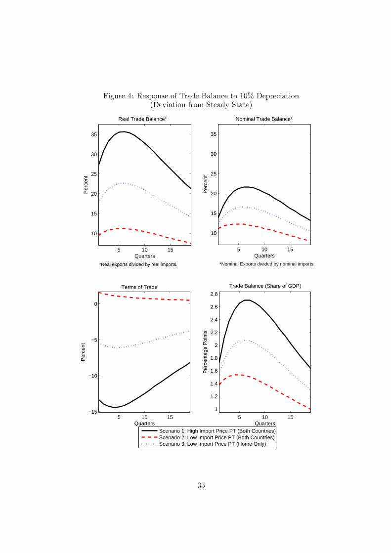
Figure 4: Response of Trade Balance to 10% Depreciation(Deviation from Steady State)
5 10 15
10
15
20
25
30
35
Per
cent
Quarters
Real Trade Balance*
5 10 15
10
15
20
25
30
35
Per
cent
Quarters
Nominal Trade Balance*
5 10 15−15
−10
−5
0
Per
cent
Quarters
Terms of Trade
5 10 15
1
1.2
1.4
1.6
1.8
2
2.2
2.4
2.6
2.8
Per
cent
age
Poi
nts
Quarters
Trade Balance (Share of GDP)
Scenario 1: High Import Price PT (Both Countries)Scenario 2: Low Import Price PT (Both Countries)Scenario 3: Low Import Price PT (Home Only)
*Real exports divided by real imports. *Nominal Exports divided by nominal imports.
35

Figure 5: Response to Equally-Sized Risk Premium Shock(Deviation from Steady State)
5 10 15
4
6
8
10
12
14
Per
cent
Quarters
Real Exchange Rate
5 10 15
10
15
20
25
30
35
Per
cent
Quarters
Real Trade Balance
5 10 150
0.5
1
1.5
2
Per
cent
age
Poi
nts
Quarters
Real Interest Rate (Annualized)
5 10 15−15
−10
−5
0
Per
cent
Quarters
Terms of Trade
5 10 15
−5
−4
−3
−2
−1
Per
cent
Quarters
Absorption
5 10 151
1.5
2
2.5
Per
cent
age
Poi
nts
Quarters
Trade Balance (Share of GDP)
Scenario 1: High Import Price PT (Both Countries)Scenario 2: Low Import Price PT (Both Countries)Scenario 3: Low Import Price PT (Home Only)
36

Figure 6: Response to Equally-Sized Risk Premium Shock with Higher Trade Elasticity(Deviation from Steady State)
5 10 15
4
6
8
10
12
14
Per
cent
Quarters
Real Exchange Rate
5 10 1520
25
30
35
40
45
Per
cent
Quarters
Real Trade Balance
5 10 150
0.5
1
1.5
2
2.5
Per
cent
age
Poi
nts
Quarters
Real Interest Rate (Annualized)
5 10 15−15
−10
−5
0
Per
cent
Quarters
Terms of Trade
5 10 15
−5
−4
−3
−2
−1
Per
cent
Quarters
Absorption
5 10 152.5
3
3.5
4
4.5
Per
cent
age
Poi
nts
Quarters
Trade Balance (Share of GDP)
Scenario 1: High Import Price PT (Both Countries)Scenario 2: Low Import Price PT (Both Countries)Scenario 3: Low Import Price PT (Home Only)
37

Figure 7: Response to Equally-Sized Risk Premium Shock with More Sluggish Demand(Deviation from Steady State)
5 10 15
4
6
8
10
12
14
Per
cent
Quarters
Real Exchange Rate
Scenario 1: High Import Price PT (Both Countries)Scenario 2: Low Import Price PT (Both Countries)Scenario 3: Low Import Price PT (Home Only)
5 10 15
10
15
20
25
30
35
Per
cent
Quarters
Real Trade Balance
5 10 150
0.5
1
1.5
2
2.5
Per
cent
age
Poi
nts
Quarters
Real Interest Rate (Annualized)
5 10 15−15
−10
−5
0
Per
cent
Quarters
Terms of Trade
5 10 15
−5
−4
−3
−2
−1
0
Per
cent
Quarters
Absorption
5 10 15
1
1.5
2
2.5
Per
cent
age
Poi
nts
Quarters
Trade Balance (Share of GDP)
38