The Adaptive Knapsack Problem with Stochastic Rewards

Taylan Ilhan, Seyed M. R. Iravani, Mark S. Daskin

Department of Industrial Engineering and Management SciencesNorthwestern University, Evanston, IL, 60208, USA

Abstract

Given a set of items with associated deterministic weights and random rewards, the AdaptiveStochastic Knapsack Problem (Adaptive SKP) maximizes the probability of reaching a predeter-mined target reward level when items are inserted sequentially into a capacitated knapsack beforethe reward of each item is realized. This model arises in resource allocation problems which permitor require sequential allocation decisions in a probabilistic setting. One particular application is inobsolescence inventory management. In this paper, the Adaptive SKP is formulated as a DynamicProgramming (DP) problem for discrete random rewards. The paper also presents a heuristic thatmixes adaptive and static policies to overcome the “curse of dimensionality” in the DP. The pro-posed heuristic is extended to problems with Normally distributed random rewards. The heuristiccan solve large problems quickly and its solution always outperforms a static policy. The numericalstudy indicates that a near-optimal solution can be obtained by using an algorithm with limitedlook-ahead capabilities.

1 Introduction

Since the seminal paper of Dantzig (1957), the knapsack problem (i.e., finding a subset of items that

maximizes the total reward while satisfying the knapsack capacity constraint) and its extensions have

been widely studied due to their practical applications. One such extension is the class of Stochastic

Knapsack Problems (SKP) with random rewards. In the Static SKP (e.g., Henig 1990 and Morton

and Wood 1998), all items are initially present and the solution is based on selecting a subset of items

that maximizes the probability of reaching a predetermined target level for the total reward. In the

Dynamic SKP (e.g., Slyke and Young, 2000; and Kleywegt and Papastavrou, 2001), the items with

random rewards and/or random sizes arrive at the system over time and the decision is whether to

accept the arrived item (to insert it into the knapsack) or to reject it after observing its actual reward

and/or size.

This paper presents an adaptive version of the Stochastic Knapsack Problem (Adative SKP),

which is defined as the problem of selecting items sequentially, one after another, with the objective of

maximizing the probability of reaching a target reward level without exceeding the knapsack capacity.

The probability distributions of the return levels for each selection are known; however, the actual

return from a selection is only revealed after making that selection. The Adaptive SKP is similar to

the Static SKP in that both problems have the same probabilistic objective function. In both the

Adaptive and Static SKPs, all items are present initially. On the other hand, unlike the Static SKP,

items are selected sequentially depending on the realizations of the random rewards in the previous

stages. Another SKP which requires sequential decision making with the objective of maximizing the

1

expected profit is the Dynamic SKP. However, in the Dynamic SKP, the items arrive at the system one

at a time and the reward realizations are observed before the accept/reject decision is made. Thus,

the Dynamic SKP and the Adaptive SKP differ with respect to these assumptions. We believe that

our study on the Adaptive SKP fills an important gap between the Static SKP and the Dynamic SKP.

The problem is motivated by obsolescence inventory management. When a manufacturing firm

makes a significant design change that eliminates a product line, or replaces an old part with a newly

designed part, the inventory of the old parts at the firm’s suppliers becomes obsolete. Since the design

change often happens before the contracts between the firm and its suppliers end, the firm is obligated

to reimburse its suppliers for their obsolete inventory. The firm audits the inventory at the suppliers’

sites before paying them their claimed amounts. In most cases, the actual reimbursement amount

differs from the amount claimed by the supplier. A recovered claim is defined to be the difference

between the value of the inventory claimed by the supplier and the actual reimbursement paid to the

supplier. These recovered claims are random and their values are not known until the suppliers are

visited.

The firm must select which supplier (or set of suppliers) among many to audit in the next audit

period. The objective is to make sure that a certain number of suppliers’ claims are audited and a

certain target recovery level is reached. After auditing a supplier and realizing the recovery amount,

the supplier that will be visited in the next period must be selected. The sequential decision of which

supplier to be audited next to increase the probability of reaching the target recovery level corresponds

to the sequential decision of which item to select in the Adaptive SKP. The inventory audit problem

is explained in greater detail in Online Appendix A. Other applications of Adaptive SKP can also be

found there.

The benefit of an adaptive solution over a static one can be shown by a simple example. Suppose,

there are only 3 items to choose from and the target level is $3. The return on item 1 is deterministic

and is $1. The return on item 2, however, is stochastic and is equally likely to be $1 or $2. Similarly,

the return on item 3 is stochastic and is equally likely to be $0 or $2. We can select only 2 items.

A simple inspection shows that an optimal static solution is to select items 1 and 2, for which the

probability of reaching the target level is 0.5. On the other hand, an adaptive policy specifies item 2

as the first selection since it dominates both items stochastically. Then, depending on its realization,

the policy picks either item 1 or item 3. The resulting probability of reaching the target level of $3 by

the adaptive policy is 0.75. As this example shows, there may be a significant increase in the optimal

value of the objective function if one uses an adaptive solution instead of a static one.

Dean et al. (2004) considered another class of the Adaptive SKP, in which the items are all

present at the beginning and have random weights with known distributions and deterministic rewards.

The problem is to find a policy that maximizes the total reward collected by inserting items one at a

2

time until the capacity of the knapsack is exceeded.

The Adaptive SKP is a special case of multi-stage stochastic programming, which is predicated

on the adaptivity in stochastic problems, (Charnes and Cooper (1959), Prekopa (1995) and Birge and

Louveaux (1997)). These problems are generally difficult. We believe that this is the first study that

analyzes adaptivity for the stochastic knapsack problem with a probabilistic objective function.

The most widely utilized tool to solve finite-horizon stochastic optimization problems is Stochas-

tic Dynamic Programming (SDP). For a general treatment of this subject, we refer the reader to

Bertsekas (1987). For some small problems, it is possible to obtain a closed form solution by solving

the Bellman equations directly. However, in many realistic problems, due to the large state space,

especially in the case of discrete optimization problems, this may not be the case. Therefore, several

look-ahead approximation methods, such as the one presented in this paper, have been developed

(see Bertsekas and Castanon (1999), Kusic and Kandasamy (2007), and Novoa and Storer (2009) for

examples).

The remainder of the paper is organized as follows. Section 2 formulates a Dynamic Program-

ming (DP) model for problems with discrete random rewards and provides analytical characteristics of

the optimal solution for a special case of the Adaptive SKP with unit weights and an unlimited num-

ber of items of each type. Section 3 presents a heuristic method for problems with discrete rewards,

which is guaranteed to yield a solution that is at least as good as the optimal static solution. Also, for

the Adaptive SKP with Normally distributed rewards, Section 4 outlines lower and upper bounding

schemes on the optimal solutions and a heuristic which integrates the previous heuristic method with

a parametric solution algorithm. Finally, Section 5 presents a numerical study to analyze the perfor-

mance of the heuristic algorithms and to identify conditions under which the value of adaptivity is

high.

2 Problem Description

Consider a knapsack with a capacity of W > 0 and a set of Ni items of each item type i ∈ N , that

can be placed in the knapsack. All items of type i ∈ N have the same deterministic weight wi. Item

j of type i ∈ N is associated with a random reward Xji . Random rewards within each type are i.i.d.

distributed (i.e. Xji ∼ Xi), and random rewards across all types are independently distributed. The

objective is to maximize the probability of reaching a target reward level of R by sequentially inserting

items into knapsack.

Suppose that the knapsack has already been partially filled with items Si for each i ∈ N , and let

xji be the realization of Xji . Define (r, w,n) to be the state of the problem, where r is the remaining

target level (R −∑

i∈N∑

j∈Sixji ), w is the remaining capacity (W −

∑i∈N |Si|wi), and n is 1 × |N |

vector whose ith entry, ni, is the number of items of type i remaining in the system (ni = Ni − |Si|).

3

In the beginning of the problem when no item has been selected, n = N = [N1, N2, . . . , N|N |]. The

problem is to find an optimal policy that inserts items sequentially into the knapsack starting from

the initial state of the problem (R,W,N). The optimal adaptive policy chooses the next item that

maximizes P(r, w,n), which is the probability of reaching the target reward level at state (r, w,n).

Assume that the reward distributions are discrete and that a type-i item can take on Ci values,

i ∈ N . Specifically, the probability that any item j of type i takes on a value xik is pik, i.e., pik =

P (Xji = xik), for k = 1, 2, . . . , Ci, and i ∈ N . Also, define ei to be a row vector composed entirely

of 0s, except that there is a 1 in the ith position. Let Pmax(r, w,n) be the optimal objective function

value of the Adaptive SKP when the system starts from state (r, w,n). The problem can be formulated

as a dynamic programming problem as follows:

Pmax(r, w,n) = maxi∈N

{ Ci∑k=1

Pmax(r − xik, w − wi,n− ei)pik}

(1)

with the following boundary conditions:

Pmax(r, w,n) = 0 w < 0; or ni < 0 for at least one i; or r > 0 , w = 0, (2)

Pmax(r, w,n) = 1 r ≤ 0 , w ≥ 0 , n ≥ 0 (3)

If the xik’s are all positive integers, then the complexity of the DP solution algorithm is

O(RW |N |CΠi=|N |i=1 (Ni+1)) where C = maxi∈N Ci since the total number of states is RWΠi=|N |

i=1 (Ni+1)

in the worst case, and the number of calculations performed at each state is bounded by |N |C. Also,

note that even if C = 2 and we have already decided which items to pick at each period (as in static

version), calculating the objective function value is #P-Hard as the problem reduces to that studied

by Kleinberg et al. (1997).

The Adaptive SKP is analogous to the bounded integer knapsack problem, which reduces to the

0/1 knapsack problem in the case in which Ni = 1, ∀i ∈ N , and becomes the unbounded knapsack

problem when Ni =∞, ∀i ∈ N . Although the bounded version may not show any particular structure,

some special cases of the unbounded version display interesting properties. For instance, if all weights

are equal for the unbounded version of the Adaptive SKP (w.l.o.g. wi = 1 ∀i ∈ N ), the problem can

be thought of as the sequential selection of W items from N item types. Since the number of available

items for each type is unlimited, the quantity terms can be eliminated from the definition of the state

(r, w,n), and we can simply use (r, w) as the state variable.

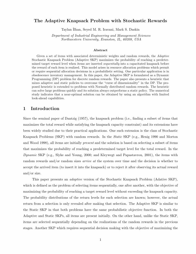
As an example of the state space, consider the unbounded and equal-weight version of the

Adaptive SKP with 4 types of items. Their reward distributions are given in Figure 1 along with

the corresponding optimal selections for each state. Even for this special case, there is no monotone

4

item x1 p1 x2 p2 item x1 p1 x2 p2

1 0 0.8 12 0.2 3 0 0.4 5 0.6

2 0 0.6 8 0.4 4 0 0.1 2 0.9

(a)

(b)

Figure 1: (a) The reward distributions for 4 item types with unit weights. The random reward of each itemhas two possible outcomes x1 and x2 with probabilities p1 and p2, respectively. (b) The DP table which givesoptimal selections at all possible remaining target levels and capacity states for an unbounded SKP with itemsdefined in Figure 2(a). Each cell corresponds to a possible problem state and contains the optimal solution atthat state; multiple items in a cell point to alternative selections, while “any” means any one of the 4 items canbe selected.

threshold level that separates the state space into regions that correspond to a particular item being

optimal. Monotone threshold levels are often desirable since they are easier to implement in practice.

When items with different weights and/or bounds on the number of items are introduced, the

decision space gets even more complex; a monotone threshold-based decision scheme may not be avail-

able for the general case of the problem. Also, the DP formulation quickly becomes computationally

intractable as the dimension of the problem increases. Thus, efficient and accurate heuristic methods

are needed for obtaining near optimal selections. Consequently, in the next section, we propose such

a heuristic method that gives the next item to select at each decision epoch.

3 A Heuristic Algorithm for Discrete Reward Distributions

To get around the “curse of dimensionality” in the DP algorithm, we propose an algorithm that uses

the solution of a number of Static SKPs to find a near-optimal solution for the Adaptive SKP. The

next two subsections introduce the Static SKP and then describe how to use it to solve the Adaptive

SKP.

5

3.1 The Formulation of the Static Stochastic Knapsack Problem

Let yij be a binary decision variable which is 1 if the jth item of type i is selected, and 0 otherwise.

Then, the Static SKP for state (r, w,n) can be formulated as follows (Morton and Wood, 1998):

Static SKP (r, w,n) : maximize P(∑i∈N

ni∑j=1

Xji yij ≥ r

)subject to: ∑

i∈Nwi

ni∑j=1

yij ≤ w

yij ∈ {0, 1} j = 1, . . . , ni ∀i ∈ N

The objective is to maximize the probability that the total reward collected is more than the target

reward level. The first constraint represents the maximum weight of the items that can be selected.

The quantity∑ni

j=1 yij gives the number of selected items of type i. The last set of constraints defines

the binary variables. Note that the objective function value of the Static SKP is a lower bound for

the objective function value of the Adaptive SKP since any static solution is also a solution to the

Adaptive SKP; i.e., even if the problem permits adaptive decision making, we can decide on all the

items to insert into the knapsack initially and not change our decisions later.

Morton and Wood (1998) and Henig (1990) develop different solution methods for the case of

the Static SKP with Normal rewards. Our study utilizes the method by Henig (1990) since it fits well

in the case of the Adaptive SKP with Normally distributed random rewards.

3.2 An L-level Heuristic

We propose an L-level heuristic that, instead of generating all possible sample paths of all feasible item

selections, the heuristic branches only L levels (each of which corresponds to an item selection) and

approximates the probabilities at each end node of the partial tree with the probability value obtained

by solving the corresponding Static SKP for the remaining part of the tree. Thus, the proposed

heuristic is only partially adaptive; to decide which item to select next, we assume L items are to be

selected adaptively and after that, the remaining knapsack capacity is to be filled in a single static

decision. However, after each selection, the algorithm reuses the heuristic to select the next item. This

continues until the knapsack is filled. In essence, the algorithm provides look-ahead capability for only

L periods instead of the entire decision horizon.

The L-period look-ahead approximation can be represented by adding a new boundary condition

to the DP model in Section 2. If the current state is (r0, w0,n0) and PS is the objective function value

of the Static SKP, then the boundary condition is

6

Pmax(r, w,n) = PS(r, w,n) : ||n0 − n||1 = L , w ≥ 0 , n ≥ 0 (4)

where ||n0 − n||1 =∑

i∈N |(n0)i − ni| and (n0)i is the ith element of the vector n0. The value of this

norm gives the number of items selected until state (r, w,n) is reached, starting from state (r0, w0,n0).

Note that the Static SKP corresponds to the heuristic with L = 0. Thus, the objective function

value obtained by solving the Adaptive SKP with the proposed algorithm is always at least as good

as that obtained by solving the Static SKP. Moreover, as the level of approximation increases, the

objective function value converges to the optimal value, since for a large enough value of L, the

boundary condition (4) becomes ignorable (or loose) and the heuristic algorithm becomes equivalent

to the original DP algorithm. The following theorem, which holds for problems with continuous as

well as discrete reward distributions, proves this result. The proofs of Theorem 1 and Theorem 2 are

presented in Online Appendix B.

Theorem 1. For any state (r, w,n), PS(r, w,n) ≤ P1(r, w,n) ≤ P2(r, w,n) ≤ . . . ≤ PL(r, w,n) ≤

PA(r, w,n), where PA, PS and Pl, l = 1, 2, . . . , L, represent the solutions of the optimal adaptive,

optimal static and l-level heuristic algorithms, respectively.

The L-level heuristic gives the next item to select and yields PL(r, w,n), an estimate for the

probability of attaining the target, each time it is run. This probability is calculated by assuming that

the algorithm will not be rerun with the remaining set of items and the updated target value after the

reward realization of the selected item. Thus, the actual probability of reaching the target level by using

the algorithm after every selection, PLactual(r, w,n), can differ from that estimated by the algorithm,

PL(r, w,n). The following theorem proves a key relationship between these two probabilities.

Theorem 2. PLactual(r, w,n) ≥ PL(r, w,n).

Our computational experience suggests that the difference between the probability of attaining

the target reward from a state using the optimal adaptive algorithm and that obtained using an L-

level approximation decreases rapidly with L. In fact, in a small example, for L = 1, over 95% of the

possible states result in no difference, and the average difference between the optimal probability and

the heuristic probability for the remaining 5% of the states is less than 0.01. For L = 2, almost 99.5%

of the states produce the same probability estimates and the average difference for the remaining states

is 0.0001. These and other similar examples of the numerical study suggest that the L-level heuristic

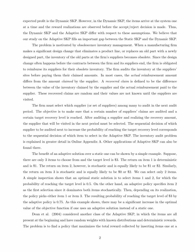
works quite well and values of 1 or 2 for L seem to be adequate for many practical purposes. Figure

2 summarizes the 1-level heuristic for problems in which the rewards have discrete distributions.

When the distribution of rewards is continuous, we cannot directly use the methods developed up

to this point. However, in the case of Normally distributed random rewards, the 1-level heuristic can

be extended in a way which makes its application to this problem very efficient and easy-to-implement.

7

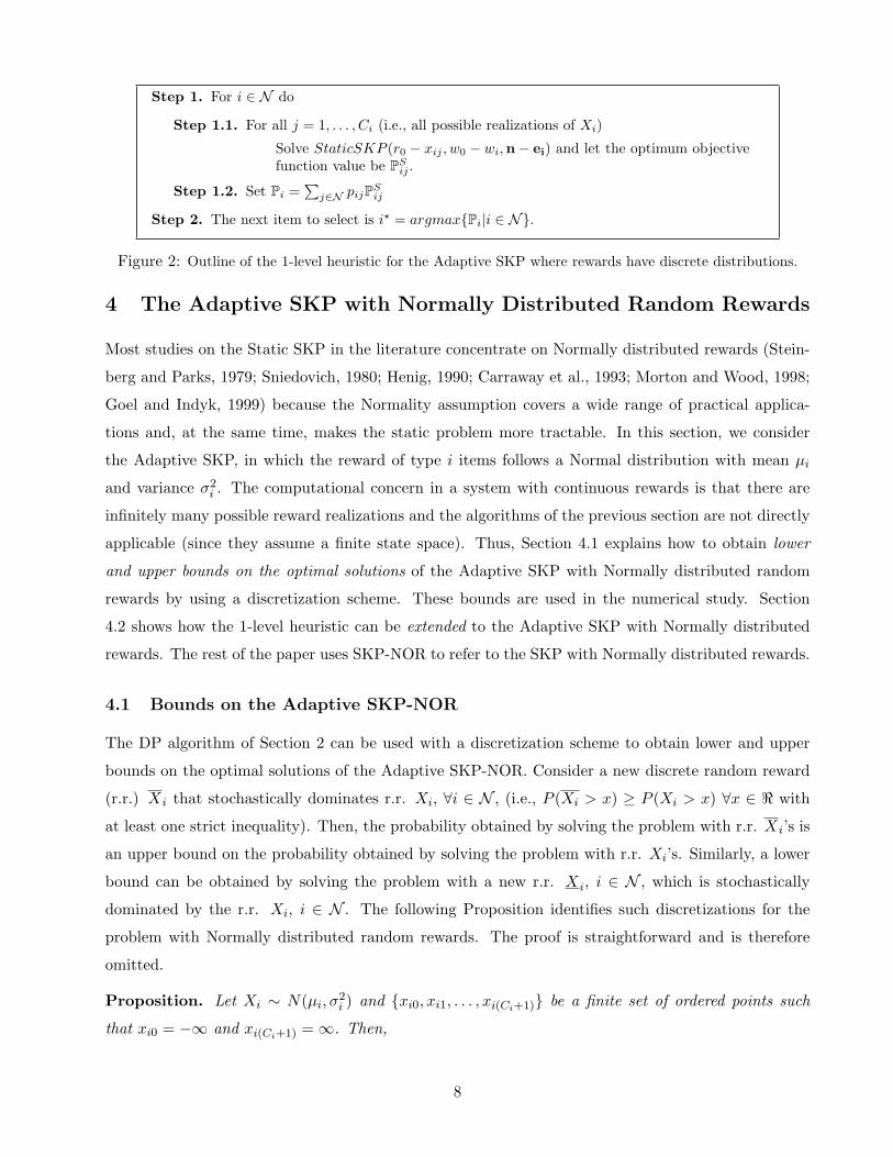
Step 1. For i ∈ N do

Step 1.1. For all j = 1, . . . , Ci (i.e., all possible realizations of Xi)

Solve StaticSKP (r0 − xij , w0 − wi,n− ei) and let the optimum objectivefunction value be PS

ij .

Step 1.2. Set Pi =∑

j∈N pijPSij

Step 2. The next item to select is i? = argmax{Pi|i ∈ N}.

Figure 2: Outline of the 1-level heuristic for the Adaptive SKP where rewards have discrete distributions.

4 The Adaptive SKP with Normally Distributed Random Rewards

Most studies on the Static SKP in the literature concentrate on Normally distributed rewards (Stein-

berg and Parks, 1979; Sniedovich, 1980; Henig, 1990; Carraway et al., 1993; Morton and Wood, 1998;

Goel and Indyk, 1999) because the Normality assumption covers a wide range of practical applica-

tions and, at the same time, makes the static problem more tractable. In this section, we consider

the Adaptive SKP, in which the reward of type i items follows a Normal distribution with mean µi

and variance σ2i . The computational concern in a system with continuous rewards is that there are

infinitely many possible reward realizations and the algorithms of the previous section are not directly

applicable (since they assume a finite state space). Thus, Section 4.1 explains how to obtain lower

and upper bounds on the optimal solutions of the Adaptive SKP with Normally distributed random

rewards by using a discretization scheme. These bounds are used in the numerical study. Section

4.2 shows how the 1-level heuristic can be extended to the Adaptive SKP with Normally distributed

rewards. The rest of the paper uses SKP-NOR to refer to the SKP with Normally distributed rewards.

4.1 Bounds on the Adaptive SKP-NOR

The DP algorithm of Section 2 can be used with a discretization scheme to obtain lower and upper

bounds on the optimal solutions of the Adaptive SKP-NOR. Consider a new discrete random reward

(r.r.) Xi that stochastically dominates r.r. Xi, ∀i ∈ N , (i.e., P (Xi > x) ≥ P (Xi > x) ∀x ∈ < with

at least one strict inequality). Then, the probability obtained by solving the problem with r.r. Xi’s is

an upper bound on the probability obtained by solving the problem with r.r. Xi’s. Similarly, a lower

bound can be obtained by solving the problem with a new r.r. Xi, i ∈ N , which is stochastically

dominated by the r.r. Xi, i ∈ N . The following Proposition identifies such discretizations for the

problem with Normally distributed random rewards. The proof is straightforward and is therefore

omitted.

Proposition. Let Xi ∼ N(µi, σ2i ) and {xi0, xi1, . . . , xi(Ci+1)} be a finite set of ordered points such

that xi0 = −∞ and xi(Ci+1) =∞. Then,

8

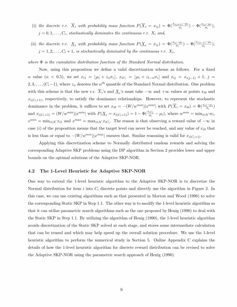
(i) the discrete r.r. Xi with probability mass function P (Xi = xij) = Φ(xi(j+1)−µi

σi) − Φ(xij−µi

σi),

j = 0, 1, . . . , Ci, stochastically dominates the continuous r.r. Xi and,

(ii) the discrete r.r. Xi with probability mass function P (Xi = xij) = Φ(xij−µi

σi) − Φ(xi(j−1)−µi

σi),

j = 1, 2, . . . , Ci + 1, is stochastically dominated by the continuous r.r. Xi,

where Φ is the cumulative distribution function of the Standard Normal distribution.

Now, using this proposition we define a valid discretization scheme as follows. For a fixed

α value (α < 0.5), we set xi1 = bµi + zασic, xiCi = bµi + z1−ασic and xij = xi(j−1) + 1, j =

2, 3, . . . , (Ci−1), where zα denotes the αth quantile of the Standard Normal distribution. One problem

with this scheme is that the new r.r. Xi’s and Xi’s must take −∞ and +∞ values at points xi0 and

xi(Ci+1), respectively, to satisfy the dominance relationships. However, to represent the stochastic

dominance in the problem, it suffices to set xi0 = −(W/wmin)|xmax| with P (Xi = xi0) = Φ(xi1−µi

σi)

and xi(Ci+1) = (W/wmin)|xmin| with P (Xi = xi(Ci+1)) = 1 − Φ(xiCiσi− µi), where wmin = mini∈N wi,

xmin = mini∈N xi1 and xmax = maxi∈N xiCi . The reason is that observing a reward value of −∞ in

case (i) of the proposition means that the target level can never be reached, and any value of xi0 that

is less than or equal to −(W/wmin)|xmax| ensures that. Similar reasoning is valid for xi(Ci+1).

Applying this discretization scheme to Normally distributed random rewards and solving the

corresponding Adaptive SKP problems using the DP algorithm in Section 2 provides lower and upper

bounds on the optimal solutions of the Adaptive SKP-NOR.

4.2 The 1-Level Heuristic for Adaptive SKP-NOR

One way to extend the 1-level heuristic algorithm to the Adaptive SKP-NOR is to discretize the

Normal distribution for item i into Ci discrete points and directly use the algorithm in Figure 2. In

this case, we can use existing algorithms such as that presented in Morton and Wood (1998) to solve

the corresponding Static SKP in Step 1.1. The other way is to modify the 1-level heuristic algorithm so

that it can utilize parametric search algorithms such as the one proposed by Henig (1990) to deal with

the Static SKP in Step 1.1. By utilizing the algorithm of Henig (1990), the 1-level heuristic algorithm

avoids discretization of the Static SKP solved at each stage, and stores some intermediate calculation

that can be reused and which may help speed up the overall solution procedure. We use the 1-level

heuristic algorithm to perform the numerical study in Section 5. Online Appendix C explains the

details of how the 1-level heuristic algorithm for discrete reward distribution can be revised to solve

the Adaptive SKP-NOR using the parametric search approach of Henig (1990).

9

5 Numerical Study

This section summarizes a numerical study designed to investigate the following three issues: (1) the

accuracy and efficiency of the 1-level heuristic, (2) the value of the optimal adaptive policy over a

static policy, and (3) the success of the 1-level heuristic in capturing the value of adaptivity. The test

problems consist of instances with |N | = 6 to 15 where Ni = 1 for all i ∈ N , and instances with

|N | = 20 to 30 where Ni ≥ 1 for all i ∈ N . In all these problem instances, the random rewards are

Normally distributed. Instances differed in terms of the item weights, the means and variances of

the item rewards, the target reward level, and the knapsack capacity. Online Appendix E provides a

detailed explanation of the factorial experiment used in the study as well as the results of the study.

Below, we summarize the highlights of those results, which all correspond to problem instances with

Normally distributed random rewards.

Accuracy of the heuristic

To measure the accuracy of the heuristic, let E = PA − P1actual be the difference between the optimal

adaptive solution obtained by the the DP algorithm (1), PA, and that of the 1-level heuristic algorithm,

P1actual.

Since we do not have an algorithm to obtain the optimal adaptive solution PA for problems with

Normally distributed rewards, we used the discretization scheme described in Section 4.1 together

with the optimal DP algorithm to obtain PA, the upper bound on the optimal adaptive solution. The

difference E = PA − P1actual is therefore an overestimation of the error E (or an underestimation of the

accuracy of the 1-level heuristic).

For problems with 6 to 15 items, the average value of E is 0.02, averaged over 530 problem

instances. The maximum value is 0.06.1 These results suggest that the 1-level heuristic approximates

the Adaptive SKP objective function very well. Furthermore, we observe that E dose not vary as the

problem size N increases from 6 to 8, 9, 10, 12 and 15. Therefore, we expect the heuristic to remain

accurate for larger problem instances as well.

Efficiency of the heuristic

The numerical analysis results in the following regression equation for the runtime of the DP algo-

rithm, when the Normal distributions are discretized based on the method in Section 4.1: runtime =

exp(−7.01 + 0.48|N | + 1.24W ). The regression equation for the runtime of the 1-level heuristic is

runtime = 0.06|N |1.2W 1.1 for cases with equal weight items, and runtime = 0.028|N |2.63W 0.46 for

cases with items of unequal weights. For example, consider a problem with |N | = 40 and W = 7,

which is the size of the inventory audit problem we observed in practice. Based on the regression1Large values of E occur when the target level and/or the level of diversity in the variability of the stochastic returns

are relatively high. Please see Online Appendix F for details.

10

models, the DP algorithm would take roughly 37 years to complete, while the maximum time of a run

of the 1-level heuristic would be approximately 43 seconds for the equal-weight cases and less than

19 minutes for unequal-weight cases. Thus, the 1-level heuristic algorithm is very time-efficient. For

details, please see Online Appendix F.

Bounds on the value of adaptivity

The value of adaptivity (VoA) is the gap between the objective function values of the optimal adaptive

and the optimal static solutions (VoA = PA − PS). This concept is important for both the optimal

and heuristic algorithms since, if the VoA is small, there is no value in using an algorithm designed to

solve the Adaptive SKP.

Again, since we do not have an algorithm to obtain the optimal adaptive solution PA for problems

with Normally distributed rewards, we use PA, the lower bound on PA, and calculate PA − PS , the

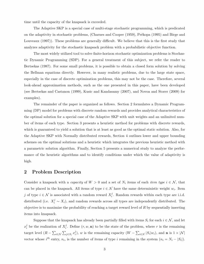
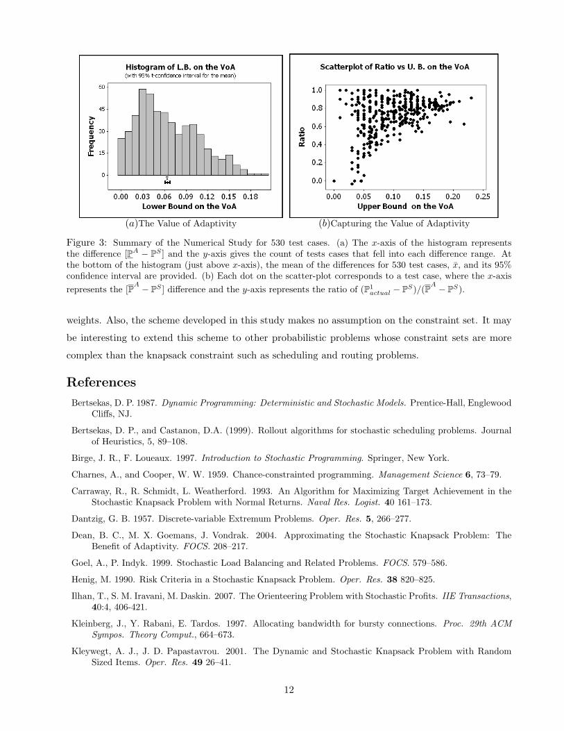
lower bound on the value of adaptivity. Figure 3(a) gives the histogram of the lower bound on the

value of adaptivity for the 530 problem instances with 6 to 15 items. The average lower bound is

0.062 and the maximum is 0.20. In 75% of the instances, the value of adaptivity exceeds 0.03. The

complete set of experiments indicates that having items with diverse risk levels (different coefficients

of variation of the rewards) increases the value of adaptivity. For details see Online Appendix G.

Capturing the value of the adaptivity

Finally, the ratio (P1actual − PS)/(PA − PS) provides an estimate of the extent to which the 1-level

heuristic captures the value of adaptivity. This ratio is between 0 and 1. The closer this ratio is to 1,

the greater the fraction of the value of adaptivity that is captured by the heuristic algorithm.

Figure 3(b) provides a scatter plot of the above ratio for the 530 problem instances with 6 to 15

items. The average ratio is 0.72. Furthermore, the ratio increases with the value of adaptivity itself.

This implies that for those problem instances with the largest value of adaptivity, the heuristic does

a good job of capturing most of the benefit associated with using the adaptive model.

6 Conclusions

This paper introduced an adaptive version of the stochastic knapsack problem in which all items are

initially present with deterministic weights and random rewards and the objective is to maximize the

probability of reaching the target reward level. We developed a DP model and an L-level heuristic

that can be used to decide on items to insert into the knapsack sequentially. This algorithm always

performs better than the optimal static algorithm and results in solutions very close to those obtained

by the optimal adaptive algorithm. The numerical results also suggest that much of the benefit of a

fully adaptive policy can be obtained by using a policy with limited look-ahead capabilities.

A possible future research direction is to analyze the Adaptive SKP in which items have random

11

(a)The Value of Adaptivity (b)Capturing the Value of Adaptivity

Figure 3: Summary of the Numerical Study for 530 test cases. (a) The x-axis of the histogram representsthe difference [PA − PS ] and the y-axis gives the count of tests cases that fell into each difference range. Atthe bottom of the histogram (just above x-axis), the mean of the differences for 530 test cases, x, and its 95%confidence interval are provided. (b) Each dot on the scatter-plot corresponds to a test case, where the x-axisrepresents the [PA − PS ] difference and the y-axis represents the ratio of (P1

actual − PS)/(PA − PS).

weights. Also, the scheme developed in this study makes no assumption on the constraint set. It may

be interesting to extend this scheme to other probabilistic problems whose constraint sets are more

complex than the knapsack constraint such as scheduling and routing problems.

References

Bertsekas, D. P. 1987. Dynamic Programming: Deterministic and Stochastic Models. Prentice-Hall, EnglewoodCliffs, NJ.

Bertsekas, D. P., and Castanon, D.A. (1999). Rollout algorithms for stochastic scheduling problems. Journalof Heuristics, 5, 89–108.

Birge, J. R., F. Loueaux. 1997. Introduction to Stochastic Programming. Springer, New York.

Charnes, A., and Cooper, W. W. 1959. Chance-constrainted programming. Management Science 6, 73–79.

Carraway, R., R. Schmidt, L. Weatherford. 1993. An Algorithm for Maximizing Target Achievement in theStochastic Knapsack Problem with Normal Returns. Naval Res. Logist. 40 161–173.

Dantzig, G. B. 1957. Discrete-variable Extremum Problems. Oper. Res. 5, 266–277.

Dean, B. C., M. X. Goemans, J. Vondrak. 2004. Approximating the Stochastic Knapsack Problem: TheBenefit of Adaptivity. FOCS. 208–217.

Goel, A., P. Indyk. 1999. Stochastic Load Balancing and Related Problems. FOCS. 579–586.

Henig, M. 1990. Risk Criteria in a Stochastic Knapsack Problem. Oper. Res. 38 820–825.

Ilhan, T., S. M. Iravani, M. Daskin. 2007. The Orienteering Problem with Stochastic Profits. IIE Transactions,40:4, 406-421.

Kleinberg, J., Y. Rabani, E. Tardos. 1997. Allocating bandwidth for bursty connections. Proc. 29th ACMSympos. Theory Comput., 664–673.

Kleywegt, A. J., J. D. Papastavrou. 2001. The Dynamic and Stochastic Knapsack Problem with RandomSized Items. Oper. Res. 49 26–41.

12

Kusic, D. and Kandasamy, N. (2007), Risk-aware limited lookahead control for dynamic resource provisioningin enterprise computing systems, Cluster Computing, 10 (4), 395-408

Morton, D. P., R. Wood. 1998. On a Stochastic Knapsack Problem and Generalizations.In Advances inComputational and Stochastic Optimization, Logic Programming and Heuristic Search. D. Woodruff, Ed.Kluwer, Boston, MA. pp. 149–168.

Prekopa, A. 1995. Stochastic Programming. Kluwer, Boston, MA.

Novoa, C. and Storer, R. (2009), An approximate dynamic programming approach for the vehicle routingproblem with stochastic demands, European Journal of Operational Research, 196 (2), 509-515.

Siniedovich, M. 1980. Preference Order Stochastic Knapsack Problems: Methodological Issues. J. Oper. Res.Soc. 31 1025–1032.

Slyke, V. R., Y. Young. 2000. Finite Horizon Stochastic Knapsacks with Applications in Yield Management.Oper. Res. 48 155–172.

Steinberg, E., M. S. Parks. 1979. A Preference Order Dynamic Program for a Knapsack Problem withStochastic Rewards. J. Oper. Res. Soc. 30 141–147.

13

Online Appendix A

Applications of Adaptive Stochastic Knapsack Problem

Inventory Audit Problem: The problem in our paper was motivated by obsolescence inventorymanagement that one of the authors encountered during his visit to the Supply Chain ManagementDepartment of a large U.S. manufacturer. What often occurs is that manufacturing firms make asignificant design change that eliminates a product line, or replaces an old part with a newly designedpart. This leads to inventory of the old parts at the firm’s suppliers becoming obsolete. Since thedesign change often happens before the contracts between the firm and its suppliers end, the firm isobligated to reimburse its suppliers for the obsolete inventory on hand.

It is clearly in the firm’s best interest to audit the inventory at the suppliers’ sites before payingthem their claimed amounts. This is due to the fact that suppliers generally overestimate the amountand the quality of the remaining inventory (with the hope of getting more money for their obsoleteinventory). To make sure that the claims are legitimate and accurate, the Obsolescence group sendsan auditor to visit each supplier’s site, and after checking the quantity and quality of the supplier’sremaining inventory, the auditor determines the value of the supplier’s inventory (according to thefirm’s regulations and the auditor’s experience). The auditor and the supplier then negotiate the finalreimbursement amount, which will be later paid to the supplier.

Available statistics at the Obsolescence group showed us that, in most cases, the actual reimbursementamount is different from the amount claimed by the supplier. A recovered claim is the differencebetween the value of the inventory claimed by the supplier and the actual reimbursement paid to thesupplier. These recovered claims are random and their values are not known until the suppliers arevisited.

When the claim is settled, the recovery amount is realized. Note that the recovery amount is onlyrevealed after the inventories are audited. Based on the history of the recovery amounts of differentsuppliers, the Obsolescence group of the firm (with the help of one of the authors) was able to identifythe distribution of recovered claims for different classes of parts and materials (e.g., bolts and nuts,plastics). Most of the distributions were approximated very well by the Normal distribution.

The Obsolescence group of the firm has a limited number of auditors who must select which supplieror suppliers (among the large list) to audit in the next audit period (e.g., two weeks). The objectiveof the Obsolescence group is to make sure that a certain number of suppliers’ claims are audited anda certain target recovery level is reached. In fact, one of the measures by which the performance ofthe Obsolescence group is evaluated is whether they reach the target recovery level specified by theObsolescence group and the manager of Supply Chain Department for the given review period (e.g.,three months). After visiting a supplier (or a set of suppliers), and realizing the recovery amount,the auditor (i.e., the Obsolescence group) must decide which supplier (or set of suppliers) s/he shouldvisit in the next period.

The Inventory Audit problem motivated our study of the “Adaptive Knapsack Problem with StochasticRewards (Adaptive SKP).” In the Inventory Audit problem

• A supplier (or a group of suppliers that are close to each other and can therefore be visited inone trip) corresponds to an item in the Adaptive SKP.

• There are a limited number of suppliers (i.e., a limited number of items in the Adaptive SKP).

14

• The time to visit a supplier (or a group of suppliers that are close to each other and can thereforebe visited in one trip) corresponds to the weight of an item in the Adaptive SKP.

• The maximum time that an auditor can spend visiting suppliers in an audit period correspondsto the capacity of the knapsack in the Adaptive SKP.

• The sequential decision of which supplier (or set of suppliers) to visit next corresponds to thesequential decision of which item to choose in the Adaptive SKP.

• The realization of the random recovered claim after a supplier is audited corresponds to therealization of the value of an item after the item is put in the knapsack.

• The primary objective of reaching the recovery target level in a quarter corresponds to theobjective of maximizing the probability of reaching a certain reward in the Adaptive SKP.

The Adaptive SKP in our paper is the first step in solving this class of problems and in gaining insightsinto developing simple but effective policies.

Other Potential Applications: Another application of the Adaptive SKP is the fishing groundselection problem (e.g., see Millar and Kiragu 1997). In this problem high yield fishing grounds needto be selected for a fishing ship. This corresponds to items to be selected and to be put in theknapsack. The yields of fishing grounds can be estimated by almost real time oceanographic analysisand historical figures. However, the yield of a fishing ground is a random variable which will notbe realized until the end of harvesting at that location. There are constraints like capacity/legallimit/target levels on the revenue that limit the number of fish caught. For example, the storagecapacity of the ship (i.e., the number of fish that can be stored in the ship) is an important constraintthat limits the revenue.2 Thus, one of the objectives of the problem is to maximize the chance ofreaching the target yield level, i.e., maximizing the probability of filling up the storage.

The “select-search-collect” nature of the Inventory Audit problem and the Fishing Ground Selectionproblem, as well as their feature of realizing a random reward after a decision is made, can also beobserved in many other situations including, civil or military reconnaissance over a large geography(see Kress and Royset 2008, Kress et al. 2006, Moser 1990), scheduling technicians for plannedmaintenance of geographically distributed equipment (see Tang et al. 2007), and talent search of asports club (see Butt and Ryan 1999). We beleive that these problems can be formulated as variantsof the Adaptive SKPs that is described in this paper.

References

Butt, S.E. and Ryan, D. M. 1999. An optimal solution procedure for the multiple tour maximum collectionproblem using column generation, Computers and Operations Research, 26, 4, 427-441.

Millar, H. H., and Kiragu, M. 1997. A time based formulation and upper bounding scheme for the selectivetraveling salesperson problem. J. Oper. Res. Soc. 48, 5, 511–518.

Kress, M., and Royset, J. O. 2008. Aerial Search Optimization Model (ASOM) for UAVs in Special Operations,Military Oper. Res., 13, 1, 23-33.

Kress, M., Baggesen, A. and Gofer, E. 2006. Probability Modeling of Autonomous Unmanned Combat AerialVehicles (UCAVs), Military Oper. Res., 11, 4, 5-24.

Moser, H. D. Jr. 1990. Scheduling and routing tactical aerial reconnaissance vehicles. Master’s thesis, NavalPostgraduate School, Monterey, CA.

2The storage capacity corresponds to the capacity of the knapsack in the Adaptive SKP.

15

Stroh, L. K., Northcraft, G. B., and Neale M. A. 2002. Organizational Behavior : A Management Challenge.Lawrence Erlbaum Associates, Mahwah, NJ.

Tang, H., Miller-Hooks, E. and Tomastik, R. 2007. Scheduling Technicians for Planned Maintenance ofgeographically Distributed Equipment. Transportation Research-Part E 43, 591-609.

Online Appendix B

Proofs of the Analytical Results

PROOF OF THEOREM 1. The proof is by induction:

Case L = 1: We will prove that PS(r, w,n) ≤ P1(r, w,n). Let q be the vector giving the number ofitems of each type selected in the optimal solution of a static problem. We can state the objectivefunction of the static problem by conditioning on item type k with qk > 0 (i.e., item k is chosen in theoptimal static solution) and setting q = q− ek as follows:

PS(r, w,n) =Ck∑j=1

P(∑i∈N

qi∑j=1

Xji > r − xkj

)pkj

The probability term inside the sum gives the probability of reaching the target level for a particularrealization of the item type k, xkj , under the solution q (i.e., the items to be chosen are in vector qat state (r − xkj , w − wk,n− ek)). We know that

PS(r − xkj , w − wk,n− ek) ≥ P(∑i∈N

qi∑j=1

Xji > r − xkj

)

since the left hand side is the value of the optimal objective function of the static problem at state(r−xkj , w−wk,n− ek) which is not restricted to select items in q. Multiplying by pkj and summingboth sides for all possible values realizations of item type k, we obtain

Ck∑j=1

PS(r − xkj , w − wk,n− ek)pkj ≥Ck∑j=1

P(∑i∈N

qi∑j=1

Xji > r − xkj

)pkj

Ck∑j=1

PS(r − xkj , w − wk,n− ek)pkj ≥ PS(r, w,n). (5)

On the other hand, for the 1-level heuristic:

P1(r, w,n) = maxi∈N

{ Ci∑j=1

PS(r − xij , w − wi,n− ei)pij}

P1(r, w,n) ≥Ck∑j=1

PS(r − xkj , w − wk,n− ek)pkj (6)

16

Thus, based on (5) and (6), we obtain

P1(r, w,n) ≥ PS(r, w,n).

Case L = l: Now, we assume that for L = l − 1 the following holds (recall that P0 = PS):

Pl−1(r, w,n) ≥ Pl−2(r, w,n) ∀(r, w,n) (7)

and prove that Pl(r, w,n) ≥ Pl−1(r, w,n). For, Pl(r, w,n) and Pl−1(r, w,n) we have

Pl(r, w,n) = maxi∈N

{ Ci∑j=1

Pl−1(r − xij , w − wi,n− ei)pij}, (8)

Pl−1(r, w,n) = maxi∈N

{ Ci∑j=1

Pl−2(r − xij , w − wi,n− ei)pij}. (9)

Based on the induction assumption (7), the right hand side of (8) is greater than that of (9). Therefore,

Pl(r, w,n) ≥ Pl−1(r, w,n) ∀(r, w,n)

which completes the induction.

PROOF OF THEOREM 2. Let T be the set of all (w,n) pairs that satisfy the following inequality

L ≥ max{∑i∈N

ni∑j=1

yij |∑i∈N

ni∑j=1

yijwi ≤ w , yij ∈ {0, 1} ∀i,∀j}

(10)

Case (w,n) ∈ T : T defines a fundamental set of states which any recursive probability calculationprocess will fall into eventually. Note that if (w,n) ∈ T and (w′,n′) ≤ (w,n), i.e., all elements in(w′,n′) are less than or equal to the corresponding elements in (w,n), then (w′,n′) ∈ T . In thiscase, the L-level heuristic is equivalent to the optimal DP algorithm since inequality (10) indicatesthat L is greater than the maximum number of items which can be inserted into the knapsack. Thus,PLactual(r, w,n) = PL(r, w,n) = PA(r, w,n).

Case (w,n) = (ω, η): Now assume that PLactual(r, ω, η) ≤ PL(r, ω, η) for any state (r, ω, η) such that(ω, η) ≤ (ω, η) with at least one strict inequality. Note that making a decision in state (ω, η) meansthat the problem moves to a state in the set of states (ω, η). Also, let u be the next item to be selectedusing the L-level heuristic. We can write the probability obtained by the algorithm as follows:

PL(r, ω,n) =Cj∑ku=0

PL−1(r − xuku , ω − wu, η − eu)puku .

17

Also, the actual probability of reaching the target level by repetitively running the L-level heuristiccan be written as follows:

PLactual(r, ω, η) =Cj∑ku=0

PLactual(r − xuku , ω − wu, η − eu)puku

≥Cj∑ku=0

PL(r − xuku , ω − wu, η − eu)puku (11)

≥Cj∑ku=0

PL−1(r − xuku , ω − wu, η − eu)puku = PL(r, ω,n) (12)

Inequality (11) is due to the assumption of the induction and inequality (12) is due to Theorem 1.

Online Appendix C

The 1-Level Heuristic Algorithm for the Adaptive SKP-NOR

For a general Static SKP, the parametric search algorithm proposed by Henig (1990) can be used toproduce a set of static solutions which contains all the optimal or close-to-optimal solutions for allpossible target profit values. We first summarize this algorithm and then present the proposed 1-levelheuristic.

The deterministic equivalent of the objective function of the Static SKP-NOR is as follows,

maximize

∑

i∈N µiyi − r√∑i∈N σ

2i yi

where yi =

∑nij=1 yij . Now, consider the following subproblem,

QA±(w,n, α) : maximize∑i∈N

(αµi ± (1− α)σ2i )yi (13)

subject to: ∑i∈N

wiyi ≤ w

yi ≤ ni, yi ∈ Z+ ∀i ∈ N

where QA− and QA+ are the problems with the (−) and (+) signs between the mean and varianceterms in the objective function (13), respectively. This is the classical bounded integer knapsackproblem and can be solved very efficiently. Solving QA− (QA+) for all α ∈ [0, 1] values generates afinite set of solutions, named EF− (EF+). Each of these solutions also represents a pair of total meanreward and total variance; i.e., ∀s ∈ EF±, (ms, vs) = (

∑i∈s µi,

∑i∈s σ

2i ). The EF− and EF+ together

constitute a convex efficient frontier of high-mean profit values in the mean-variance domain. Also, ifthere is a feasible solution s with

∑i∈s µi ≥ r, this efficient frontier is guaranteed to contain the optimal

point for any target reward level r; otherwise, the optimal solution is not necessarily contained in theconvex efficient frontier. Henig (1990) shows that the points on the convex frontier contain solutionswhich approximate the optimal solutions very well and, in general, the number of points is quitesmall. In Online Appendix D, we develop a polynomial-time algorithm for the static SKP with equal

18

weights, wi = w ∀i ∈ N . Using this algorithm, the efficient frontier can be constructed in polynomialtime. Solving the subproblems with such a polynomial-time algorithm increases the effectiveness ofthe 1-level heuristic substantially since the complexity of the 1-level heuristic is dependent on thecomplexity of the solution method used for the subproblems.

To solve QA±(w,n, α) for all α ∈ [0, 1], we start from two pairs of mean-variance points and recursivelycalculate new α values and solve new subproblems. This is based on the fact that, if the objectivefunction values for α1 and α2 are equal, that is QA±(w,n, α1) = QA±(w,n, α2), then QA±(w,n, α) =QA±(w,n, α1) for all α ∈ [α1, α2] (see Proposition 3 in Ilhan et al. 2007). Thus, the algorithm itselfchooses the α values which are needed to construct the subproblems.

Now, we can transform the algorithm for rewards with discrete distributions given in Figure 2 into the1-level heuristic for Normally distributed rewards. The idea of the 1-level heuristic is as follows. First,assuming we have selected item i, we find the best solutions in terms of objective function (13) for allpossible values of the new target level r = r − Xi, or equivalently for all possible realizations of therandom reward of the selected item i, Xi = x ∈ (−∞,∞). This is achieved by using the parametricsearch algorithm above. Second, by using the solutions obtained in the first step, we calculate theprobability of reaching the target level r by selecting item i. After repeating these steps for all items inN , we select the item with the highest probability. Below, we elaborate on each step of the algorithm.

Step1. Finding the best (m,v) points: Solve the subproblems QA±(w − wi,n− ei, α) for all possible αvalues to construct a set of mean-variance pairs. Then, construct a solution set S of the followingform:

S =

(m∗1, v

∗1) is the best for r ∈ [−∞, a1)

(m∗2, v∗2) is the best for r ∈ [a1, a2)

...(m∗|S|, v

∗|S|) is the best for r ∈ [a|S−1|,∞)

Step 2. Probability calculation: The probability of reaching the target level value r if item i is selectedcan be obtained as follows:

P1i (r, w,n) =

∫ ∞−∞

PS(r − x,w − wi,n− ei)fi(x)dx (14)

The previous step provides the optimal or close to the optimal solutions to the static problemfor all possible target values. For each interval of x and corresponding (m∗s, v

∗s) pair in S,

PS(r − x,w − wi,n− ei) can be calculated by using the Normal distribution. Thus, equation(14) can be approximated as follows:

P1i (r, w,n) ≈

s=|S|∑s=1

∫ as

as−1

Φ(m∗s + x− r√

v∗s

)fi(x)dx

where Φ(x) is the c.d.f. of the Standard Normal and fi(x) is the p.d.f. of Normal distributionwith parameters µi and σ2

i . In this study, we approximate this integral by discretizing fi(x)with equal-probability values, pdscrt = 0.001. Letting D = 1/pdscrt, xd = µi+Φ−1(pdscrtd)σi and(m∗d, v

∗d) be the mean-variance pair that corresponds to r = r − xd in S, then P1

i (r, w,n) can be

approximated by pdscrt∑D

d=0 Φ(m∗

d−r+xd√v∗d

).

19

After repeating Steps 1 and 2 for all i ∈ N , the next item to select is i? = argmax{P1i |i ∈ N}.

Online Appendix D

The Static SKP with Equal Weights – A Polynomial-Time Algorithm

The algorithm presented here is based on the study by Henig (1990). When all weights are identical(e.g., wi = 1, ∀i ∈ N ), the Static SKP-NOR reduces to the following formulation:

Maximize

∑i∈N µiyi −R√∑

i∈N σ2i yi

subject to: ∑i∈N

yi ≤W (15)

yi ∈ {0, 1} ∀i ∈ N (16)

This problem is a special case of the SKP, for which DP algorithms exist (see Morton and Wood 1998).However, we develop a polynomial algorithm by using the idea that, if there is a feasible solution s

such that∑

i∈s µi > R, the optimal solution is one of the solutions obtained by solving the followingproblem for all α ∈ [0, 1] (see Henig 1990):

Maximize∑i∈N

[αµi − (1− α)σ2i ]yi (17)

subject to: constraints (15) and ( 16)

The solution to this subproblem for any given α value can easily be obtained. We calculate thecoefficients of the items; i.e., zi = αµi − (1 − α)σ2

i . If zi < 0, then we set the corresponding yi’sto 0. If there are less than W positive zi values, then we set all corresponding yi to 1; otherwise,we sort the zi’s in non-ascending order and set the first W yi’s to 1. The particular values of zi’sare not important. The solution is dependent only on the signs and the relative values of the zi’s.Thus, if the signs and the order of the coefficients do not change for an interval of α values, then theoptimal solution stays the same for that particular interval. We can generate all the intervals of α byevaluating all pairs of coefficients and signs of individual coefficients, as follows.

1. The relative positions of zi and zj change if the α value passes the following point where zi = zjfor j > i:

αµi − (1− α)σ2i = αµj − (1− α)σ2

j =⇒ α =σ2j − σ2

i

µj − µi + σ2j − σ2

i

2. The sign of zi changes if α passes the following point:

αµi − (1− α)σ2i = 0 =⇒ α =

σ2i

µi + σ2i

There are |N |2/2 values of α for the first case and |N | values of α for the second case. Consideringα = 0 and α = 1, we have at most |N |2/2 + |N |+ 2 different α values. Moreover, some of them may

20

not be in the interval [0, 1] since there may be cases with µi > µj and σi < σj . If we generate all αvalues and combine them in an ordered set, then each successive pair of α values forms an interval inwhich the optimal solution stays the same. The complexity of finding all α values is O(|N |2) . Thecomplexity of solving the problem with the objective function (17) for each α value is O(|N | log |N |)if we use the Quicksort algorithm. It follows that the complexity of the algorithm which solves theoriginal problem is O(|N |3 log |N |). Finally, if there is no feasible solution s such that

∑i∈s µi > R,

then we can still apply this algorithm by simply changing the (−) sign to a (+) sign between the termsin objective function (17). However, in this case, the algorithm does not guarantee the optimality ofthe solution to the problem.

Online Appendix E

The Design of the Numerical Analysis

Our first objective is to test the efficiency and accuracy of the 1-level heuristic by comparing itssolution with the optimal static solution and with bounds on the optimal adaptive solutions. Oursecond objective is to identify the conditions under which it is valuable to employ an adaptive policyover a static one. All algorithms used in this study are coded in C++ and run on a PC with a Pentium4 CPU and 512 MB of RAM.

The test problems are composed of items with Normally distributed rewards. Thus, only the means andvariances of the rewards are needed to characterize the randomness in the problem. We concentrateon Normally distributed rewards since the Normal distribution has a wide range of applications inpractice and, since there are efficient algorithms for the Static SKP-NOR that enable us to carry outthe tests effectively.

We designed two sets of problems. The first set consists of problems containing 6 to 15 item types, forwhich we can obtain the optimal adaptive solution using our DP algorithm. The second set consistsof problems containing 20 to 30 types for which we cannot obtain the optimal adaptive solution butfor which we can still find the optimal static solution and compare it against the 1-level heuristic. Thedetailed description of the construction of these sets is given in the following two subsections.

E.1. The Design of Problems with 6 to 15 Item Types

One of the objectives of the numerical study is to analyze the effect of the different levels of problemparameters. We first examine a set of problems with equal weight items (i.e., wi = 1). This ismotivated by the fact that in the inventory audit problem, the time that auditors spend in a supplieris usually one day. Furthermore, the case with equally-weighted items allows us to analyze the effectof the stochasticity of rewards, without the confounding impact of different item weights.

E.1.1. The Design of the Equal-Weight Cases

We created test problems with N = 6, 8, 9, 10, 12, and 15. In all test problems, each type containedone item only; i.e., Ni = 1, i ∈ N . Thus, the number of item types and the total number of itemsavailable were the same.

We used items with Normally distributed rewards. We created 53 different groups of item types bycombining different sets of coefficients of variation (c.v.) and different sets of mean reward levels.These sets are given in Figure 4, where there are 10 sets of c.v. values, 10 sets of mean rewardvalues, resulting in 100 possible mean/c.v combinations. For example, the combination of two mean

21

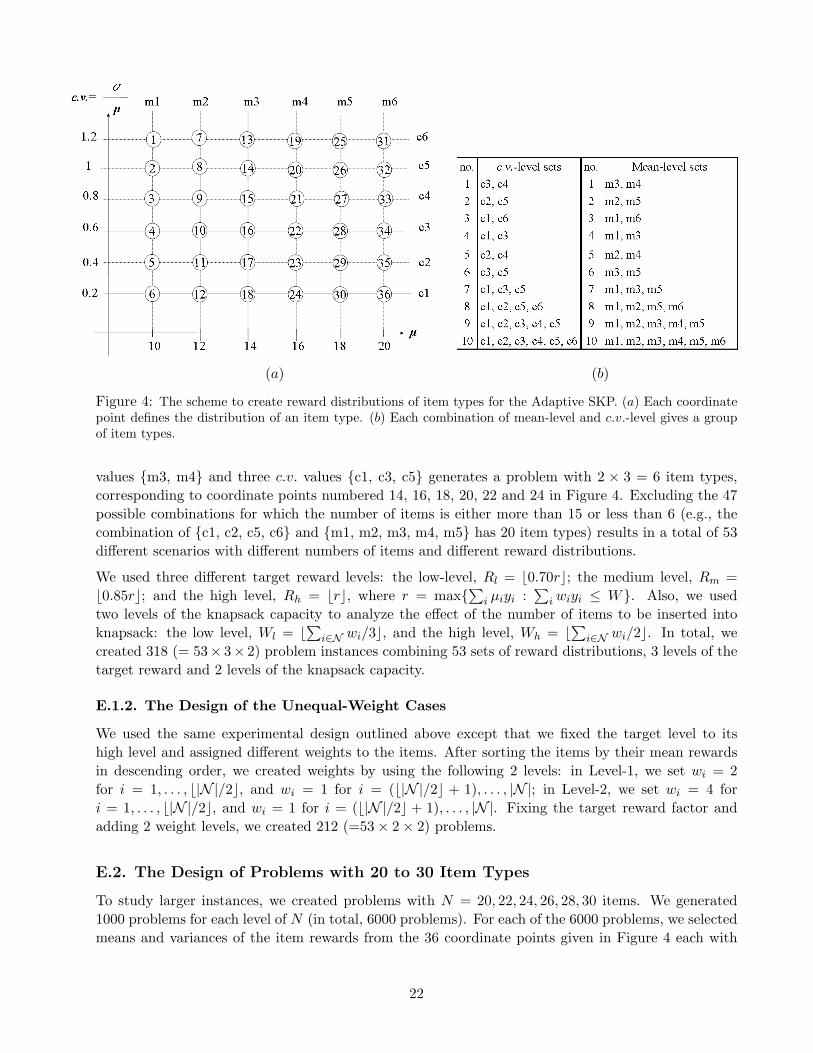
(a) (b)

Figure 4: The scheme to create reward distributions of item types for the Adaptive SKP. (a) Each coordinatepoint defines the distribution of an item type. (b) Each combination of mean-level and c.v.-level gives a groupof item types.

values {m3, m4} and three c.v. values {c1, c3, c5} generates a problem with 2 × 3 = 6 item types,corresponding to coordinate points numbered 14, 16, 18, 20, 22 and 24 in Figure 4. Excluding the 47possible combinations for which the number of items is either more than 15 or less than 6 (e.g., thecombination of {c1, c2, c5, c6} and {m1, m2, m3, m4, m5} has 20 item types) results in a total of 53different scenarios with different numbers of items and different reward distributions.

We used three different target reward levels: the low-level, Rl = b0.70rc; the medium level, Rm =b0.85rc; and the high level, Rh = brc, where r = max{

∑i µiyi :

∑iwiyi ≤ W}. Also, we used

two levels of the knapsack capacity to analyze the effect of the number of items to be inserted intoknapsack: the low level, Wl = b

∑i∈N wi/3c, and the high level, Wh = b

∑i∈N wi/2c. In total, we

created 318 (= 53× 3× 2) problem instances combining 53 sets of reward distributions, 3 levels of thetarget reward and 2 levels of the knapsack capacity.

E.1.2. The Design of the Unequal-Weight Cases

We used the same experimental design outlined above except that we fixed the target level to itshigh level and assigned different weights to the items. After sorting the items by their mean rewardsin descending order, we created weights by using the following 2 levels: in Level-1, we set wi = 2for i = 1, . . . , b|N |/2c, and wi = 1 for i = (b|N |/2c + 1), . . . , |N |; in Level-2, we set wi = 4 fori = 1, . . . , b|N |/2c, and wi = 1 for i = (b|N |/2c + 1), . . . , |N |. Fixing the target reward factor andadding 2 weight levels, we created 212 (=53× 2× 2) problems.

E.2. The Design of Problems with 20 to 30 Item Types

To study larger instances, we created problems with N = 20, 22, 24, 26, 28, 30 items. We generated1000 problems for each level of N (in total, 6000 problems). For each of the 6000 problems, we selectedmeans and variances of the item rewards from the 36 coordinate points given in Figure 4 each with

22

probability 1/36. In other words, we randomly picked N pairs of mean reward and c.v. values fromthe set of 36 points (allowing the same point to be selected more than once). Also, item weights wereset to 1, and for each problem the capacity and the target reward levels were generated by settingW = N/2 and R = 0.9×max{

∑i µiyi :

∑i yi ≤W}.

Online Appendix F

The Evaluation of the 1-Level Heuristic

In this appendix, we evaluate the efficiency and accuracy of the 1-level heuristic. Since we did nothave an optimal algorithm for solving the Adaptive SKP-NOR, we used the DP algorithm in Section2 along with the discretization scheme in Section 4.1 to obtain upper bounds on the optimal adaptiveprobabilities. To solve the Static SKP-NOR with equal weights, we used the polynomial time algorithmpresented in Online Appendix D for the unit-weight version of this problem. To solve the Static SKP-NOR with unequal weights, we used the algorithm by Henig (1990).

F.1. Equal-Weight Case

This subsection evaluates the accuracy and the efficiency of the 1-level heuristic for test problems withequally-weighted items.

F.1.1. The Accuracy of the Heuristic for Problems with 6 to 15 ItemsAs mentioned before, the probability obtained by the 1-level heuristic at each step is not the realprobability of reaching the target reward, since we use the probability values approximated by thestatic sub-problems instead of the actual ones. Thus, to estimate the real probabilities for the policyobtained by the 1-level heuristic (P1

actual), we used Monte Carlo simulation. For each problem, wesimulated 2000 cases to estimate the resulting probability of reaching the target value under the policyobtained by the 1-level heuristic. The result of each run was a success or a failure in attaining thetarget reward level. The total number of successes divided by the total number of runs is an estimateof the true probability of reaching the target under the policy obtained by our 1-level heuristic.

In the absence of an optimal algorithm for solving the Adaptive SKP-NOR, we used the discretizationscheme and obtained PA, the upper bound on the optimal adaptive probability (PA). The differencebetween PA and P1

actual is an overestimation of PA − P1actual (i.e., an underestimation of the accuracy

of the 1-level heuristic).

The average of the gaps between the solutions obtained by the upper bounds on the optimal adaptivesolution and the 1-level heuristic (i.e., PA−P1

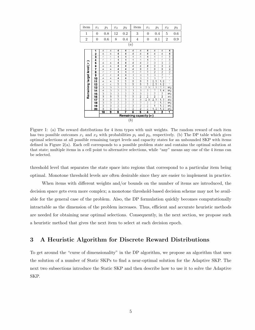
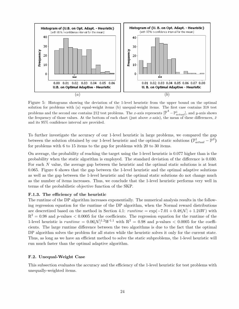
actual) is 0.019 with a standard deviation of 0.015. Figure5(a) shows that the maximum deviation of the 1-level heuristic from the optimal adaptive solution is0.06. Large deviations occur when the target level and/or the level of diversity in c.v.s are relativelyhigh. These results show that the 1-level heuristic results in solutions that are very close to the optimaladaptive solutions.

F.1.2. The accuracy of the heuristic for problems with 20 to 30 itemsDue to the large state space of the DP model we could not test the proposed 1-level heuristic againstthe optimal adaptive policy for problems with more than 15 items with unit-weights. However, in theexperiments with 6 to 15 items, the gap between the solution to the 1-level heuristic and the upperbound on the optimal adaptive solution did not change as N increased from 6 to 8, 9, 10, 12, and 15.Thus, we expect that the 1-level heuristic also performs well for larger problems.

23

(a) (b)

Figure 5: Histograms showing the deviation of the 1-level heuristic from the upper bound on the optimalsolution for problems with (a) equal-weight items (b) unequal-weight items. The first case contains 318 testproblems and the second one contains 212 test problems. The x-axis represents [PA−P1

actual], and y-axis showsthe frequency of those values. At the bottom of each chart (just above x-axis), the mean of these differences, xand its 95% confidence interval are provided.

To further investigate the accuracy of our 1-level heuristic in large problems, we compared the gapbetween the solution obtained by our 1-level heuristic and the optimal static solutions (P1

actual − PS)for problems with 6 to 15 items to the gap for problems with 20 to 30 items.

On average, the probability of reaching the target using the 1-level heuristic is 0.077 higher than is theprobability when the static algorithm is employed. The standard deviation of the difference is 0.030.For each N value, the average gap between the heuristic and the optimal static solutions is at least0.065. Figure 6 shows that the gap between the 1-level heuristic and the optimal adaptive solutionsas well as the gap between the 1-level heuristic and the optimal static solutions do not change muchas the number of items increases. Thus, we conclude that the 1-level heuristic performs very well interms of the probabilistic objective function of the SKP.

F.1.3. The efficiency of the heuristicThe runtime of the DP algorithm increases exponentially. The numerical analysis results in the follow-ing regression equation for the runtime of the DP algorithm, when the Normal reward distributionsare descretized based on the method in Section 4.1: runtime = exp(−7.01 + 0.48|N | + 1.24W ) withR2 = 0.98 and p-values < 0.0005 for the coefficients. The regression equation for the runtime of the1-level heuristic is runtime = 0.06|N |1.2W 1.1 with R2 = 0.98 and p-values < 0.0005 for the coeffi-cients. The large runtime difference between the two algorithms is due to the fact that the optimalDP algorithm solves the problem for all states while the heuristic solves it only for the current state.Thus, as long as we have an efficient method to solve the static subproblems, the 1-level heuristic willrun much faster than the optimal adaptive algorithm.

F.2. Unequal-Weight Case

This subsection evaluates the accuracy and the efficiency of the 1-level heuristic for test problems withunequally-weighted items.

24

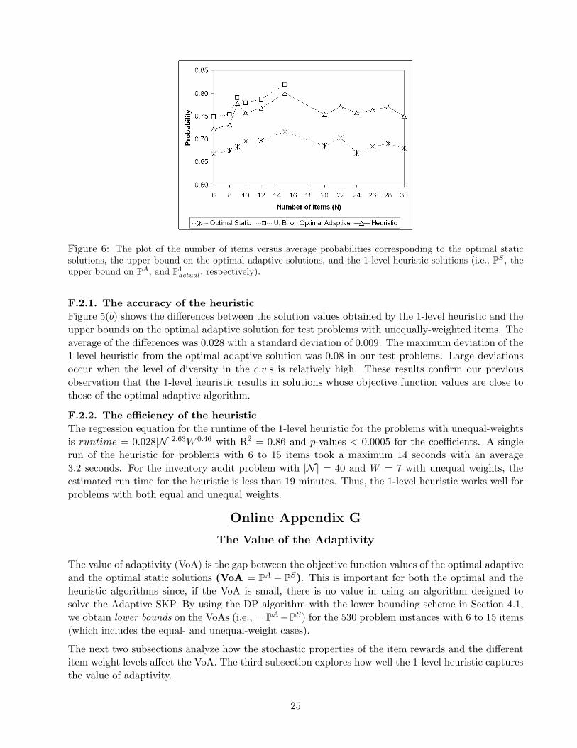
Figure 6: The plot of the number of items versus average probabilities corresponding to the optimal staticsolutions, the upper bound on the optimal adaptive solutions, and the 1-level heuristic solutions (i.e., PS , theupper bound on PA, and P1

actual, respectively).

F.2.1. The accuracy of the heuristicFigure 5(b) shows the differences between the solution values obtained by the 1-level heuristic and theupper bounds on the optimal adaptive solution for test problems with unequally-weighted items. Theaverage of the differences was 0.028 with a standard deviation of 0.009. The maximum deviation of the1-level heuristic from the optimal adaptive solution was 0.08 in our test problems. Large deviationsoccur when the level of diversity in the c.v.s is relatively high. These results confirm our previousobservation that the 1-level heuristic results in solutions whose objective function values are close tothose of the optimal adaptive algorithm.

F.2.2. The efficiency of the heuristicThe regression equation for the runtime of the 1-level heuristic for the problems with unequal-weightsis runtime = 0.028|N |2.63W 0.46 with R2 = 0.86 and p-values < 0.0005 for the coefficients. A singlerun of the heuristic for problems with 6 to 15 items took a maximum 14 seconds with an average3.2 seconds. For the inventory audit problem with |N | = 40 and W = 7 with unequal weights, theestimated run time for the heuristic is less than 19 minutes. Thus, the 1-level heuristic works well forproblems with both equal and unequal weights.

Online Appendix G

The Value of the Adaptivity

The value of adaptivity (VoA) is the gap between the objective function values of the optimal adaptiveand the optimal static solutions (VoA = PA − PS). This is important for both the optimal and theheuristic algorithms since, if the VoA is small, there is no value in using an algorithm designed tosolve the Adaptive SKP. By using the DP algorithm with the lower bounding scheme in Section 4.1,we obtain lower bounds on the VoAs (i.e., = PA−PS) for the 530 problem instances with 6 to 15 items(which includes the equal- and unequal-weight cases).

The next two subsections analyze how the stochastic properties of the item rewards and the differentitem weight levels affect the VoA. The third subsection explores how well the 1-level heuristic capturesthe value of adaptivity.

25

G.1. The Effect of Stochasticity on the VoA

The design of the reward distributions in Figure 4 enables us to test the value of using the adaptivemodel over the static model under many different conditions, in addition to several target reward andknapsack capacity levels. Specifically, the design in Figure 4 enables us to observe the effects of thedispersion, variety and average of the c.v.s and mean values of the random rewards on the value ofthe adaptive policy over the static one.

• Dispersion of c.v.s: This factor provides insight into how the VoA changes as the differencebetween the c.v. values of the items (i.e., the variability in the item rewards) increases althoughtheir average stays the same. To examine this, we compare 120 problems created with {c3,c4}, {c2, c5} and {c1, c6} (which are low, medium and high levels of dispersion in the c.v.s,respectively). For these cases, the average c.v. value remains at 0.7 while the range of c.v.’sincreases from 0.02 (low value) to 1 (high value). For each level of dispersion in the c.v.s, wehave 40 instances; i.e., 24 equal-weight instances plus 16 unequal-weight instances. We performeda two-sample t-test of the null hypothesis “H0 : dispersion level of c.v.s has no effect on VoA” forevery pair of this factor and calculated the corresponding confidence intervals. If the confidenceinterval for the difference between the adaptive and the static policy values includes zero, there isno statistically significant difference in the average of the VoA under the different c.v. scenarios{c3, c4}, {c2, c5} and {c1, c6}.

• Variety of c.v.s: As the variety level increases, there are more items with different c.v. valuesalthough their average stays the same. Comparing problems created with {c1,c6}, {c1, c2, c5,c6} and {c1, c2, c3, c4, c5, c6} enables us to analyze the effect of low, medium and high levels ofvariety in the c.v.s. The difference between “dispersion” and “variety” is that in the latter casethere are more items with different levels of c.v.s than in the previous case. The low, medium andhigh levels of this factor correspond to instances generated by 4, 7 and 6 mean levels (countingthe valid combinations of c.v. and mean level sets), respectively, and 10 different target, weightand capacity levels. Thus, the low, medium and high levels contain 40, 70 and 60 instances,respectively. The null hypothesis “H0 : variety level of c.v.s had no effect” was again tested forevery pair of levels of this factor.

• Average of c.v.s: We compared problems created from the following three scenarios for c.v.s, {c1,c3}, {c2, c4} and {c3, c5}, which correspond to gradually increasing the average c.v. values (0.4,0.6 and 0.8, respectively) although the difference between the c.v. values stays the same. Thisenabled us to observe the impact of increasing c.v.s (or risk levels) for all item rewards together.Note that in the previous two cases (i.e., the dispersion and the variety) the average c.v. levelsstays the same. There are 40 instances for each level of the average of the c.v.s.

• We did similar comparisons for the mean rewards. Problems created with {m3, m4}, {m2, m5}and {m1, m6} were used to analyze the effect of the dispersion in mean rewards; problemscreated with {m1, m6}, {m1, m2, m5,m6}, {m1, m2, m3, m4, m5, m6} were used to analyzethe effect of the variety in mean rewards; and problems created with {m1, m3}, {m2, m4} and{m3, m5} were used to analyze the effect of the average of the mean rewards.

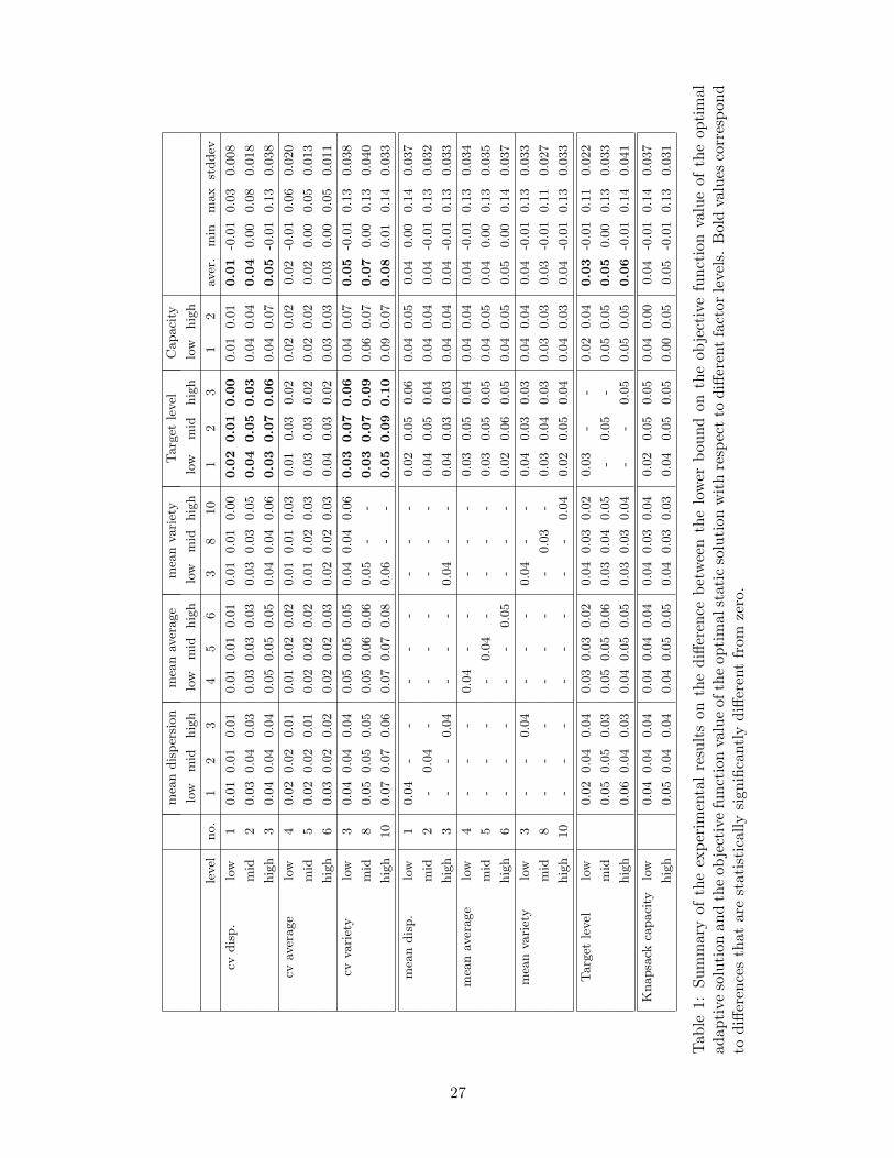
Table 1 summarizes the results for the difference between the lower bound on the probability of reachingthe target reward using the optimal adaptive policy and the probability of reaching the target usingthe optimal static policy. The average and the maximum differences are 0.05 and 0.14, respectively.For about 75% of the problems, the benefit of the adaptive policy over the static policy (i.e., the VoA)is more than 0.03.

26

mea

ndis

per

sion

mea

nav

erage

mea

nva

riet

yTarg

etle

vel

Capaci

ty

low

mid

hig

hlo

wm

idhig

hlo

wm

idhig

hlo

wm

idhig

hlo

whig

h

level

no.

12

34

56

38

10

12

31

2av

er.

min

max

stddev

cvdis

p.

low

10.0

10.0

10.0

10.0

10.0

10.0

10.0

10.0

10.0

00.0

20.0

10.0

00.0

10.0

10.0

1-0

.01

0.0

30.0

08

mid

20.0

30.0

40.0

30.0

30.0

30.0

30.0

30.0

30.0

50.0

40.0

50.0

30.0

40.0

40.0

40.0

00.0

80.0

18

hig

h3

0.0

40.0

40.0

40.0

50.0

50.0

50.0

40.0

40.0

60.0

30.0

70.0

60.0

40.0

70.0

5-0

.01

0.1

30.0

38

cvav

erage

low

40.0

20.0

20.0

10.0

10.0

20.0

20.0

10.0

10.0

30.0

10.0

30.0

20.0

20.0

20.0

2-0

.01

0.0

60.0

20

mid

50.0

20.0

20.0

10.0

20.0

20.0

20.0

10.0

20.0

30.0

30.0

30.0

20.0

20.0

20.0

20.0

00.0

50.0

13

hig

h6

0.0

30.0

20.0

20.0

20.0

20.0

30.0

20.0

20.0

30.0

40.0

30.0

20.0

30.0

30.0

30.0

00.0

50.0

11

cvva

riet

ylo

w3

0.0

40.0

40.0

40.0

50.0

50.0

50.0

40.0

40.0

60.0

30.0

70.0

60.0

40.0

70.0

5-0

.01

0.1

30.0

38

mid

80.0

50.0

50.0

50.0

50.0

60.0

60.0

5-

-0.0

30.0

70.0

90.0

60.0

70.0

70.0

00.1

30.0

40

hig

h10

0.0

70.0

70.0

60.0

70.0

70.0

80.0

6-

-0.0

50.0

90.1

00.0

90.0

70.0

80.0

10.1

40.0

33

mea

ndis

p.

low

10.0

4-

--

--

--

-0.0

20.0

50.0

60.0

40.0

50.0

40.0

00.1

40.0

37

mid

2-

0.0

4-

--

--

--

0.0

40.0

50.0

40.0

40.0

40.0

4-0

.01

0.1

30.0

32

hig

h3

--

0.0

4-

--

0.0

4-

-0.0

40.0

30.0

30.0

40.0

40.0

4-0

.01

0.1

30.0

33

mea

nav

erage

low

4-

--

0.0

4-

--

--

0.0

30.0

50.0

40.0

40.0

40.0

4-0

.01

0.1

30.0

34

mid

5-

--

-0.0

4-

--

-0.0

30.0

50.0

50.0

40.0

50.0

40.0

00.1

30.0

35

hig

h6

--

--

-0.0

5-

--

0.0

20.0

60.0

50.0

40.0

50.0

50.0

00.1

40.0

37

mea

nva

riet

ylo

w3

--

0.0

4-

--

0.0

4-

-0.0

40.0

30.0

30.0

40.0

40.0

4-0

.01

0.1

30.0

33

mid

8-

--

--

--

0.0

3-

0.0

30.0

40.0

30.0

30.0

30.0

3-0

.01

0.1

10.0

27

hig

h10

--

--

--

--

0.0

40.0

20.0

50.0

40.0

40.0

30.0

4-0

.01

0.1

30.0

33

Targ

etle

vel

low

0.0

20.0

40.0

40.0

30.0

30.0

20.0

40.0

30.0

20.0

3-

-0.0

20.0

40.0

3-0

.01

0.1

10.0

22

mid

0.0

50.0

50.0

30.0

50.0

50.0

60.0

30.0

40.0

5-

0.0

5-

0.0

50.0

50.0

50.0

00.1

30.0

33

hig

h0.0

60.0

40.0

30.0

40.0

50.0

50.0

30.0

30.0

4-

-0.0

50.0

50.0

50.0

6-0

.01

0.1

40.0

41

Knapsa

ckca

paci

tylo

w0.0

40.0

40.0

40.0

40.0

40.0

40.0

40.0

30.0

40.0

20.0

50.0

50.0

40.0

00.0

4-0

.01

0.1

40.0

37

hig

h0.0

50.0

40.0

40.0

40.0

50.0

50.0

40.0

30.0

30.0

40.0

50.0

50.0

00.0

50.0

5-0

.01

0.1

30.0

31

Tab

le1:

Sum

mar

yof

the

expe

rim

enta

lre

sult

son

the

diffe

renc

ebe

twee

nth

elo

wer

boun

don

the

obje

ctiv

efu

ncti

onva

lue

ofth

eop

tim

alad

apti

veso

luti

onan

dth

eob

ject

ive

func

tion

valu

eof

the

opti

mal

stat

icso

luti

onw

ith

resp

ect

todi

ffere

ntfa

ctor

leve

ls.

Bol

dva

lues

corr

espo

ndto

diffe

renc

esth

atar

est

atis

tica

llysi

gnifi

cant

lydi

ffere

ntfr

omze

ro.

27

The tests show that the target reward level is an important factor affecting the value of the adaptivesolutions. If the target level is low, the average of the lower bound on the difference between the staticsolution and the adaptive solution is 0.04 and if it was high, the corresponding average is 0.07. Theestimated increase in the difference from the low target level to the high target level is 0.036 with a95% confidence interval of (0.028, 0.044), which does not contain 0. When the target level is low, theprobability of reaching the target level is close to 1 so that the possibility of an improvement due tothe use of the adaptive model is small.

The dispersion and variety of the c.v.s also impact the value of adaptivity. When the c.v. dispersionlevel changes from low to high, the value of adaptivity increases by an average of 0.045 with a 95%confidence interval of (0.032, 0.058). When we have items with more diverse variance levels, the abilityto select between items with high and low variances becomes more valuable. Also, when the c.v. varietylevel changes from low to high, the value of the adaptivity increases by an average of 0.028 with a95% confidence interval of (0.012, 0.044). The problem instance that shows the maximum value ofadaptivity (0.15 difference between objective function values) has the high level of the c.v. variety andthe high level of the target reward.

Each of the remaining conditions exhibits no statistically significant effect on the value of the adaptivepolicy. Obviously, using a stochastic model may be valuable over a deterministic model if there israndomness in a knapsack problem. However, our experiments indicate that the mean values of theitem rewards, the average level of c.v.s and the knapsack capacity do not have a direct effect on thevalue of an adaptive model over a static model. An adaptive stochastic model seems to have valuewhen the problem has a diversity in risk beyond having randomness, which provides the ability tochange the amount of risk taken depending on the target level.

G.2. Equal-Weight Cases vs. Unequal-Weight Cases

We compared the values of adaptivity obtained for each unequal-weight case with the correspondingequal-weight case. The 95% confidence interval of (−0.018, 0.005) around the mean of the differencesbetween the cases with unit weights and the cases with Level-1 weights contains 0. Thus, we cannotconclude that the value of adaptivity is higher or lower for the cases with Level-1 weights. On theother hand, the average difference between the VoA for the cases with unit weights and the VoA forthe cases with Level-2 weights was −0.021 with a 95% Confidence Interval of (−0.032,−0.011). Theseresults suggest that, when items are not equally-weighted, the difference between item weights can havea statistically significant effect on the value of adaptivity (compared to cases with equally-weighteditems).

G.3. Capturing the Value of Adaptivity

We compared the 1-level heuristic results for the 530 problems with 6 to 15 items against both theoptimal adaptive and optimal static solutions to see if the 1-level heuristic performs closer to theoptimal adaptive or to the optimal static algorithm. For this purpose, we use the Ratio of VoAs ,which is (P1

actual − PS)/(PA − PS). If the ratio is close to 1, then the 1-level heuristic performs closeto the optimal adaptive solution. If the upper bound on the VoA is 0, we set the ratio to 0.

In general, the ratios are closer to 1 than to 0, with a mean value of 0.72. The ratio consistentlyincreases as the VoA increases and most of the problems for which the ratio is close to 0 are the oneswhich have almost no value of adaptivity. These results show that the 1-level heuristic successfullycaptures most of the value in solving the SKP in an adaptive manner.

28