Relaxation Analysis for the

Dynamic Knapsack Problem with Stochastic Item Sizes

Daniel Blado Alejandro TorielloH. Milton Stewart School of Industrial and Systems Engineering

Georgia Institute of Technology

Atlanta, Georgia 30332

deblado at gatech dot edu atoriello at isye dot gatech dot edu

January 19, 2018

Abstract

We consider a version of the knapsack problem in which an item size is random and revealedonly when the decision maker attempts to insert it. After every successful insertion the decisionmaker can dynamically choose the next item based on the remaining capacity and available items,while an unsuccessful insertion terminates the process. We build on a semi-infinite relaxationintroduced in previous work, known as the Multiple Choice Knapsack (MCK) bound. Our firstcontribution is an asymptotic analysis of MCK showing that it is asymptotically tight underappropriate assumptions. In our second contribution, we examine a new, improved relaxationbased on a quadratic value function approximation, which introduces the notion of diminishingreturns by encoding interactions between remaining items. We compare this bound to othersfrom the literature, including the best known pseudo-polynomial bound. The quadratic boundis theoretically more efficient than the pseudo-polynomial bound, yet empirically comparable toit in both value and running time.

1 Introduction

The deterministic knapsack problem is a fundamental discrete optimization model that has beenstudied extensively in areas such as computer science, operations research and industrial engineer-ing. Recently, knapsack models under uncertainty have been the subject of much research, bothto model resource allocation problems with uncertain parameters, and as a subproblem in moregeneral discrete optimization problems under uncertainty, such as stochastic integer programming.In particular, dynamic knapsack problems, where decisions occur sequentially and problem param-eters may be revealed dynamically, have been a topic of ongoing interest; such models have seenmany applications, including in scheduling [9], equipment replacement [10], and machine learning[14, 15, 24].

The dynamic knapsack model variant we analyze here has stochastic item sizes that are onlyrevealed to the decision maker after they attempt to insert an item. Throughout the process, theremaining items and their respective size distributions are available, and the process only continuesif an attempted item’s realized size fits within the remaining capacity. This differs from morestatic models, in which the decision maker decides on a particular subset of items ahead of time,essentially attempting to insert the set all at once, and the question is whether that set fits in theknapsack with a desired probability, e.g. [12].

1

Having the flexibility to choose subsequent items in light of the revealed sizes of previous itemsintuitively can lead to a higher overall expected value than a more static approach. However, thisadded freedom raises the complexity of the problem both in practice and theory. A feasible solutionto this problem now takes the form of a policy that dictates what the decision maker should attemptto insert under any possible state, as opposed to deciding on a subset of items to insert a priori.Such added difficulty motivates work to develop reasonably tight and tractable relaxations, as wellas high-quality, efficient policies. In particular, [4] introduced a Multiple-Choice Knapsack (MCK)semi-infinite relaxation that stems from an affine value function approximation; our goal in thispaper is to provide theoretical analysis to understand this relaxation’s quality and to improve itwhen a gap remains. Our contributions can be summarized as:

i) We prove the MCK bound is asymptotically tight by comparing it to a natural greedy policyunder two distinct but related regimes. Therefore, the computationally efficient MCK modelprovides increasingly tighter bounds for instances with larger numbers of items. In addition,this result provides an alternative proof of the asymptotic optimality of the greedy policy,recently shown in [2].

ii) We introduce a quadratic relaxation that builds on MCK by encoding interactions betweenpairs of remaining items, and show that it maintains polynomial solvability. For instances witha medium number of items, where MCK has a gap but dynamic programming is intractable,the quadratic bound is comparable to the best known pseudo-polynomial bound [24] in bothvalue and running time, even making considerable improvement in some cases.

The remainder of the paper is organized as follows. We conclude this section with a briefliterature review. Section 2 states the problem formulation and preliminaries, including the relevantprevious results. Section 3 provides the asymptotic analysis of the MCK bound. Section 4 thenstudies the improved quadratic bound, examining structural results and outlining a computationalstudy. Section 5 concludes, and an appendix contains proofs and computational experiment datanot included in the main article.

1.1 Literature Review

The knapsack problem and its generalizations have been studied for over half a century, havingapplications in areas as varied as budgeting, finance, and scheduling; see [19, 25]. The knapsackproblem under various forms of uncertainty has specifically received attention as well; [19, Chapter14] surveys some of these results. In general, optimization under uncertainty can be modeled viaeither a static approach that chooses a solution a priori, or a dynamic (sometimes called adaptive[7, 8, 9]) approach that chooses a solution sequentially based on realized parameters. Examplesof a priori knapsack models with uncertain item values include [5, 16, 27, 31, 32], a priori modelswith uncertain item sizes include [11, 12, 20, 21], and an a priori model with both uncertain valuesand sizes can be found in [26]. Dynamic models for knapsacks with uncertain item sizes include[3, 7, 9, 10, 14, 15], while [18] study a dynamic model with uncertain item values. Another variant,the stochastic and dynamic knapsack, examines the case where items are not initially given butrather arrive dynamically according to a stochastic process; see [22, 23, 28] .

Regarding our dynamic variant of the stochastic knapsack problem in particular, [10] first stud-ied the version with exponentially distributed item sizes, and showed that the greedy policy thatinserts items based on their value-to-mean-size ratio is optimal in this case. More recently, [7, 9]studied the problem in its full generality, providing two linear programming bounds with polynomi-ally many variables, showing that both were within a constant multiplicative gap, and investigating

2

greedy approximate policies. Afterwards, [14, 15, 24] researched bounds under the assumption ofinteger size support, evaluating the performance of LP relaxations of pseudo-polynomial size anddeveloping randomized policies based on their optimal solutions. Their framework applied to vari-ants beyond the problem studied here, including correlated random item values, preemption, andthe multi-armed bandits problem with budgeted learning.

Using value function approximations to obtain relaxations of dynamic programs dates back to[1, 6, 30, 33]. The results in [4] provide the technique’s first application for a stochastic knapsackmodel, evaluating various bounds. The investigation of asymptotic properties of relaxations via acomparison to a natural greedy policy was initially empirically suggested by computational resultsin [4]; the asymptotic optimality of the greedy policy was then shown by [2] using informationrelaxation duality techniques.

2 Problem Formulation and Preliminaries

As with the deterministic knapsack problem, suppose we have a knapsack with capacity b > 0 anditem set N := 1, 2, . . . , n. Each item i has a deterministic value ci > 0. Item sizes are nowindependent random variables Ai ≥ 0, each drawn from an arbitrary but known distribution. Anitem size is realized after the decision maker attempts to insert it. When attempting to insertan item i, the decision maker is faced with two outcomes: If i fits, value ci is collected and theremaining capacity is updated; or, i is too large, and the process ends, i.e. we only allow one failedinsertion. A policy stipulates what item to insert, and may depend on the remaining items andremaining capacity. The objective is to maximize the expected value of successfully inserted items.

This problem can be modeled as a dynamic program (DP). Each possible state the decisionmaker faces can be defined by the non-empty set of remaining items M ⊆ N and remainingcapacity s ∈ [0, b]. For a given state (M, s), the possible actions allowed consist of attempting toinsert an item i ∈M . If we define v∗M (s) as the optimal expected value at state (M, s), the Bellmanrecursion is

v∗M (s) = maxi∈M

P(Ai ≤ s)(ci + E[v∗M\i(s−Ai)|Ai ≤ s]), (1)

with the base case v∗∅(s) = 0. Intuitively speaking, should the attempted item i have size greaterthan s, we collect nothing, but should it fit we collect both the item’s value ci and the optimalexpected value of the subsequent state, that is, (M \ i, s − Ai). The linear programming (LP)formulation of this problem is

minv

vN (b) (2a)

s.t. vM∪i(s) ≥ P(Ai ≤ s)(ci + E[vM (s−Ai)|Ai ≤ s]), (2b)

i ∈ N, M ⊆ N \ i, s ∈ [0, b] (2c)

vM : [0, b]→ R+, M ⊆ N. (2d)

This is a doubly infinite LP, as there are a continuum of constraints over all s ∈ [0, b], and variablesvM are real-valued functions.

Notation To simplify notation, we denote an item size’s cumulative distribution function byFi(s) := P(Ai ≤ s) for i ∈ N , and its complement by Fi(s) := P(Ai > s). Additionally, the meantruncated size of item i ∈ N at capacity s ∈ [0, b] is the quantity Ei(s) := E[mins,Ai] [7, 9, 34];this quantity frequently comes up in the rest of the paper. Intuitively, if the remaining capacity iss, we should not care about the distribution of item i’s size above s, as any such realization willresult in a failed insertion.

3

2.1 Multiple-Choice Knapsack Bound

The doubly infinite LP (2) cannot in general be efficiently solved. However, any feasible solutionto the LP provides a valid upper bound on the optimal solution. Earlier work in [4] examines thebound resulting from approximating the optimal value function as

vM (s) ≈ qs+ r0 +∑i∈M

ri, (3)

where r0 represents the inherent value of keeping the knapsack available, ri is the value of havingitem i available, and q is the marginal value of the remaining capacity.

Proposition 2.1 ([4]). The best possible bound given by approximation (3) is the solution of thesemi-infinite LP

minq,r

qb+ r0 +∑i∈N

ri (4a)

s.t. qEi(s) + r0Fi(s) + ri ≥ ciFi(s), ∀ i ∈ N, s ∈ [0, b] (4b)

r, q ≥ 0. (4c)

The finite-support strong dual of (4) provides an approximation with a more intuitive problemstructure:

maxx

∑i∈N

∑s∈[0,b]

cixi,sFi(s) (5a)

s.t.∑i∈N

∑s∈[0,b]

xi,sEi(s) ≤ b (5b)

∑i∈N

∑s∈[0,b]

xi,sFi(s) ≤ 1 (5c)

∑s∈[0,b]

xi,s ≤ 1, ∀ i ∈ N (5d)

x ≥ 0, x has finite support. (5e)

This is a two-dimensional, fractional multiple-choice knapsack problem [19], henceforth referred toas the MCK bound. MCK is efficiently solvable for many common distributions, such as thosewhose cumulative distribution function is piecewise convex [4]. This work also includes an exten-sive computational study indicating that MCK becomes tighter as the number of items increases,motivating the asymptotic analysis in Section 3. However, many instances still exhibit a noticeablebound/policy gap; Section 4 thus examines a new bound that tightens this gap while maintainingcomputational efficiency.

2.2 Pseudo-Polynomial Bound

When item sizes have integer support, [24] proposes a pseudo-polynomial (PP) bound,

maxx

∑i∈N

b∑s=0

cixi,sFi(s) (6a)

s.t.∑i∈N

b∑s=σ

xi,sFi(s− σ) ≤ 1, σ = 0, . . . , b (6b)

4

b∑s=0

xi,s ≤ 1, i ∈ N (6c)

x ≥ 0, (6d)

which arises from the value function approximation

vM (s) ≈∑i∈M

ri +s∑

σ=0

wσ. (7)

When available, this bound is provably tighter than MCK [4] and serves as a benchmark to de-termine the strength of polynomially solvable bounds. We use both PP and MCK to gauge thestrength of the new quadratic bound in Section 4.

3 Asymptotic Analysis

We first define necessary terms and assumptions used in the analysis. The greedy ordering [10]sorts items with respect to their value-to-mean-size ratio, ci/E[Ai], in non-increasing order. Thegreedy policy attempts to insert items in this order until either all of the items have successfullybeen inserted or an attempted insertion violates capacity.

Our analysis in this section slightly generalizes the original problem setup by assuming thedecision maker has access to an infinite sequence of items sorted according to the greedy ordering;in other words, N = 1, 2, . . . = N and ci/E[Ai] ≥ ci+1/E[Ai+1]. We can thus study the asymptoticbehavior of policy and bound as functions of capacity only. This problem setup differs from resultsin [2], where the item set N also grows as part of the analysis; our results are arguably strongerin the sense that they do not depend on the order in which items become available to the decisionmaker (as the entire sequence is always available). To further compare our techniques to [2], weinclude a second analysis under their regime below in Section 3.1.

We must further clarify how we define v∗ for the infinite item case, as the original formulationis defined recursively for finitely many items. Let v∗[n](b) and MCK[n](b) denote the value functionand MCK bound, respectively, with respect to the first n items according to the greedy ordering.Note that both of these quantities are monotonically nondecreasing sequences with respect to n,and for fixed b, v∗[n](b) ≤ MCK[n](b) holds for every n [4]. We thus define v∗N (b) := limn→∞ v

∗[n](b),

and similarly define MCK(b) := limn→∞MCK[n](b). To show that both of these limits exist andare finite, it suffices to find a finite upper bound for MCK[n](b) for all n; such a bound is providedbelow.

Let Greedy(b) refer to the expected policy value as a function of the knapsack capacity b; notethis is already well defined for the infinite item case since the greedy ordering is assumed to befixed. We use the greedy policy to show that MCK (5) is asymptotically tight; in the process, thisalso proves that the greedy policy is asymptotically optimal, yielding an alternate proof to [2]. Toproceed with the analysis, we make the following assumptions.

Assumption 3.1. Among all items i,

i) expectation is uniformly bounded from above and below, 0 <¯µ ≤ E(Ai) ≤ µ, and

ii) variance is uniformly bounded from above, Var(Ai) ≤ V ,

for some constants¯µ, µ, V .

5

Assumption 3.2. The sum of item values grows fast enough:∑

i≤k ci = Ω(k12+ε). For example,

having a uniform non-zero lower bound for all ci suffices.

Assumption 3.3.c′0 := sup

s∈[0,∞)i=1,2,...

[E[Ai|Ai > s]− s

]<∞. (8)

Intuitively, this last assumption governs the behavior of the size distributions’ tails; we discusssome examples below.

We separate the analysis into four auxiliary results. The first result is a probability statementused in later proofs.

Remark 3.4. Denote E[Ai] by the shorthand Ei. Then,

Ei − Ei(s)

Fi(s)= E[Ai|Ai > s]− s.

Proof. By definition,

Ei − Ei(s)

Fi(s)=

Ei − (Fi(s)s+ Fi(s)E[Ai|Ai ≤ s])Fi(s)

=Ei − E[Ai|Ai ≤ s]

Fi(s)+ (E[Ai|Ai ≤ s]− s).

The fraction in the right hand side above simplifies to

Ei − E[Ai|Ai ≤ s]Fi(s)

=(Ei − E[Ai|Ai ≤ s])Fi(s)

Fi(s)Fi(s)

=E[Ai|Ai ≤ s]Fi(s)(Fi(s)− 1) + E[Ai|Ai > s]Fi(s)Fi(s)

Fi(s)Fi(s)

= E[Ai|Ai > s]− E[Ai|Ai ≤ s].

The second step establishes an upper bound for MCK.

Lemma 3.5. Let bk :=∑

i≤k E[Ai]. Under Assumptions 3.1 and 3.3, for any n,

MCK[n](bk) ≤∑i≤k

ciP(Ai ≤ bk) + c0,

where c0 is a constant independent of k and n.

Proof. Fix k and n. Without loss of generality, we may assume n ≥ k, since we can establish theupper bound MCK[n](bk) ≤ MCK[k](bk) for all n ≤ k. For the sake of brevity we will abuse somenotation in the proof, denoting bk as b (and E[Ai] as Ei). Recalling (4) is the dual to the MCKbound (5), we proceed to find a dual feasible solution.

We start at the case i ≥ k. Let us set ri = 0, which corresponds to allotting no value to itemsafter item k in the greedy ordering. We must satisfy

qEi(s) + r0Fi(s) ≥ ciFi(s), ∀s ∈ [0,∞).

Motivated by the possible case where Fi(s) = 1, if we set q = ck/Ek ≥ ci/Ei, variable r0 must nowsatisfy

r0Fi(s) ≥ ciFi(s)− qEi(s) = ci − ciFi(s)− qEi(s) +( ckEk

)Ei −

( ckEk

)Ei

6

=[ci −

( ckEk

)Ei]

+ckEk

[Ei − Ei(s)

]− ciFi(s).

Should Fi(s) = 0, the constraint reduces to 0 ≥ 0. Thus, assuming Fi(s) 6= 0, there are three termsin the right hand side of the above inequality. Since r0 must upper bound such constraints for alli and s, we drop the first and last terms, both of which are non-positive. This yields constraints

r0 ≥ckEk

(Ei − Ei(s)

Fi(s)

)=ckEk

(E[Ai|Ai > s]− s

), ∀i ≥ k, s ∈ [0, b], (9)

where the equality holds by Remark 3.4.Next, we examine the case i < k. To find a valid choice of ri, we again are motivated by the

(possible) case where Fi(s) = 1, which implies

qEi(s) + r0Fi(s) + ri ≥ ciFi(s) =⇒ qEi + ri ≥ ci =⇒ ri ≥ ci −ckEk

Ei.

This is a non-negative value for ri since the greedy ordering yields

ri = ci −ckEk

Ei = Ei[ ciEi− ck

Ek

]≥ 0.

These choices of q and ri present a dual objective of the desired form:

qb+∑i∈N

ri = b( ckEk

)+∑i<k

Ei( ciEi− ck

Ek

)=∑i<k

ci −∑i<k

Ei( ckEk

)+ b( ckEk

)=∑i<k

ci −∑i<k

Ei( ckEk

)+∑i≤k

Ei( ckEk

)=∑i<k

ci + Ek

( ckEk

)=∑i≤k

ci =∑i≤k

ciFi(b) +∑i≤k

ciFi(b).

Furthermore, noting that Fi(b) = P(Ai > bk) = P(Ai >∑

i≤k Ei) ≤ P(Ai > k¯µ) ≤ Ei/k

¯µ ≤ µ/k

¯µ,

the sum∑

i≤k ciFi(b) can be upper bounded with

∑i≤k

ciFi(b) ≤∑i≤k

c1EiE1

Fi(b) ≤c1µ

¯µ

∑i≤k

Fi(b) ≤c1µ

2k

¯µ2k

=c1µ

2

¯µ2

,

which is constant with respect to k and i. Therefore, the second sum in the objective can be upperbounded and absorbed into the c0 term.

It thus suffices to show that a valid choice for dual variable r0 exists such that it is constantwith respect to k (and bk), for then we can also absorb r0 into c0, completing the proof. Continuingthe case where i < k, the constraints in (4) require that r0 satisfy

r0Fi(s) ≥ ciFi(s)− ri − qEi(s).

Should Fi(s) = 0, the choices of ri and q reduce the constraint to 0 ≥ 0. If Fi(s) 6= 0, the conditionis

r0 ≥ciFi(s)− ri − qEi(s)

Fi(s)=ciFi(s)− ci + ckEi

Ek− ckEi(s)

Ek

Fi(s)

=−ciFi(s) + ck

Ek[Ei − Ei(s)]

Fi(s)= −ci +

ckEk

[E[Ai|Ai > s]− s],

7

where the last equality follows from Remark 3.4. This holds if r0 satisfies

r0 ≥ckEk

[E[Ai|Ai > s]− s], ∀i ∈ [n], s ∈ [0, b],

which is exactly constraint (9) in the case that i ≥ k. Recalling Assumption 3.3, setting r0 = c1c′0/E1

satisfies (9) for all values of i and s. Since r0 is constant with respect to k and n (and bk), we canset c0 = c1(µ

2/¯µ2 + c′0/E1). This result holds for all n, completing the proof.

The above result proves that the limit MCK(bk) exists and is finite. Let Sk denote the sum ofthe first k sizes according to the greedy ordering, Sk :=

∑i≤k Ai. The expected value of the greedy

policy when restricted to the first k items under capacity bk is trivially∑

i≤k ciP(Si ≤ bk). This isa lower bound for the actual greedy policy, which considers all of the items instead of the first k.By Lemma 3.5, for each bk we have a lower bound of

Greedy(bk)

MCK(bk)≥

∑i≤k ciP(Si ≤ bk)∑

i≤k ciP(Ai ≤ bk) + c0.

The ratio in the left-hand side above is always at most 1 since the numerator is a feasible policyand the denominator is an upper bound on the optimal policy. We next examine the asymptoticnature of the lower bound.

Lemma 3.6. Under Assumptions 3.1 and 3.2,

limk→∞

∑i≤k ciP(Si ≤ bk)∑

i≤k ciP(Ai ≤ bk) + c0= 1.

Proof. It suffices to show that the numerator can be lower bounded by∑

i≤k ci − O(√k), as the

result will then follow from Assumption 3.2 and the trivial upper bound P(Ai ≤ bk) ≤ 1. Recallingbk =

∑i≤k

Ei = E[Sk], we first upper bound the probability

P(Si > bk) = P(Si − E[Si] > E[Sk − Si]) ≤ P(|Si − E[Si]| > E[Sk − Si])

= P((Si − E[Si])2 > (E[Sk − Si])2) ≤

Var(Si)( ∑i<j≤k

E[Ai])2 ≤ iV

(k − i)2¯µ2, (10)

where the second inequality comes from Markov’s (or Chebyshev’s) inequality. Next, we defineupper bound c := c1µ/E1 ≥ ci. Let j be some number such that j < k, to be determined. Using(10) yields ∑

i≤kciP(Si ≤ bk) =

∑i≤j

ciP(Si ≤ bk) +∑j<i≤k

ciP(Si ≤ bk)

≥∑i≤j

ci

[1− iV

(k − i)2¯µ2

]+∑j<i≤k

ci(1− P(Si > bk)) ≥∑i≤k

ci −cV

¯µ2

∑i≤j

i

(k − i)2− c(k − j)

≥∑i≤k

ci −cV

¯µ2

j+1∫0

x

(k − x)2dx− c(k − j) =

∑i≤k

ci −cV

¯µ2

[ j + 1

k − j − 1+ ln(k − j − 1)− ln k

]− c(k − j)

=∑i≤k

ci −cV

¯µ2

[k −√k√k

+ ln(√k)− ln k

]− c(√k + 1) =

∑i≤k

ci −O(√k).

8

The second to last equality occurs when we make the suitable choice k − j − 1 =√k, that is,

j = k −√k − 1. Letting (k − j − 1) be of order

√k consequently minimizes the order of the

second and third terms (those that are not∑

i≤k ci) to be of order√k; one can easily check that

choosing a different power of k will lead to an overall higher order for either the second term orthird term.

Lemma 3.6 examines the limit in terms of the number of items in the knapsack, a discretesequence dependent on k, but we wish to show the asymptotic property over all positive values b.Therefore, we formalize this result in terms of the increasing knapsack capacity b.

Theorem 3.7. Suppose we are given a greedily ordered infinite sequence of items satisfying As-sumptions 3.1, 3.2, and 3.3. Then,

Greedy(b)

MCK(b)→ 1 as b→∞. (11)

Proof. Given b, let bk− and bk+ refer to the nearest bk values below and above b, respectively. Then,trivially Greedy(b) ≥ Greedy(bk−). Further, MCK(b) ≤ MCK(bk+) since the objective of MCK isnondecreasing with b. Therefore we obtain

Greedy(b)

MCK(b)≥

Greedy(bk−)

MCK(bk+)≥

Greedy(bk−)

MCK(bk−) + ck+Fk+(bk+)≥

Greedy(bk−)

MCK(bk−) + c0→ 1.

The second inequality follows from decomposing the upper bound of MCK(bk+) into the upperbound of MCK(bk−) and the additional objective term involving item k+, while the last inequalityfollows because every ciFi(b) term can be upper bounded by a constant, as in the proof of Lemma3.6. The final expression goes to 1 by Lemma 3.6.

This result is consistent with the computational experiments in [4] that spurred our analysis,which tested the MCK bound under the following distributions: bounded discrete distributionswith two to five breakpoints, uniform, and exponential. Under all such distributions, the datasuggested that MCK and Greedy were asymptotically equivalent; comparing with Assumption 3.3:

• Under the discrete and uniform distributions, the sizes exhibit uniformly bounded support.Thus, the value c′0 defined in Assumption 3.3 exists and is finite (it is simply the upper boundon item size support), and the theorem applies.

• Under the exponential distribution, suppose E[Ai] = 1/λi. By the memoryless property, forany i and any s,

E[Ai|Ai > s]− s = (1/λi + s)− s = 1/λi <∞.

Thus, if the item sizes have a uniformly bounded mean, c′0 exists and is finite, and the theoremapplies.

According to the analysis in the proof of Lemma 3.6, if the sum of the item values growsas Ω(g(k)), the numerator of the fraction is lower bounded by Ω(g(k) −

√k); hence, the rate of

convergence is O(√k/g(k)). For example, if g(k) = k, the rate of convergence is O(k−1/2).

Corollary 3.8. The rate of convergence of (11) is O(√k/g(k)), where

∑i≤k ci = Ω(g(k)).

Assumption 3.3 is not always straightforward to check for a particular distribution, so we providean alternate set of sufficient conditions.

9

Proposition 3.9. Suppose the following hold:

i) Among those items with bounded support, there exists a uniform finite upper bound.

ii) Among all items i without bounded support, there exists an α > 0 such that

(a) P(Ai > t) ≥ e−αt for all t > 0, and

(b) Mi(α) := E[eαAi ] ≤ M(α) <∞; that is, the moment generating function at α exists andis uniformly bounded among such i.

iii) For all i, P(Ai > 0) ≥ z > 0. Note that for continuous distributions we can trivially takez = 1 since Ai is nonnegative.

Then,c′0 = sup

s∈[0,∞)i=1,2,...

[E[Ai|Ai > s]− s

]<∞.

Proof. There are three cases for each item: an item has bounded support, unbounded support andzero probability of being 0, or unbounded support and nonzero probability of being 0. For eachcase we exhibit a uniform bound across all items of that case, then set c′0 to the maximum of thesethree absolute upper bounds.

The bounded support case is taken care of by the first condition. For the second case, considerany item i. Since Ai is a nonnegative random variable, by Markov’s inequality

P(Ai > t) = P(eαAi > eαt) ≤ E[eαAi ]

eαt.

Further, recall for nonnegative random variables the identity E[Ai] =∫∞t=0 F(t)dt. Thus, for the

random variable (Ai − s),

E[Ai − s|Ai > s] =

∫∞t=0 P(Ai − s > t)dt

P(Ai > s)≤ 1

P(Ai > s)

∫ ∞t=0

E[eαAi ]

eα(t+s)dt

=E[eαAi ]

P(Ai > s)eαs

( 1

α

)≤ M(α)

e−αseαs

( 1

α

)=

M(α)

α<∞.

The first inequality follows from the Markov bound presented earlier on P(Ai > t + s), while thesecond inequality follows from both parts of the second assumption. This provides an absoluteupper bound for E[Ai − s|Ai > s] for all values of s ∈ (0,∞), taking care of the second case ofitems.

For the third case of items, it suffices to uniformly bound the case that s = 0. By the thirdassumption (and earlier assumption of uniformly bounded mean) we have

E[Ai − 0|Ai > 0] =E[Ai]

P(Ai > 0)≤ µ

z<∞.

Since the above analysis does not depend on the choice of i, this completes the proof.

10

3.1 A Second Regime

The results in [2] provide an alternate asymptotic analysis of the greedy policy in which itemsbecome available to the decision maker incrementally as capacity grows; when the number of itemsk grows, each new item is added to the same subset of already available items. The authors examinean upper bound based on information relaxation techniques, and provide a case analysis dependenton the growth of capacity as a function of the number of available items, to show under whatconditions the greedy policy is asymptotically optimal. Motivated by this result, we show that theMCK bound allows for similar conclusions.

Consider denoting Greedy(k, b(k)) as the expected value gained from the greedy policy givenk items and b(k) capacity; we now make explicit the fact that b is a function of k. Similarly, letMCK(k, b(k)) be the optimal value of MCK given k items and b(k) capacity. Unlike the previousframework, we no longer make any assumption about the ordering of items, implying in particularthat items are possibly re-sorted for each k to calculate Greedy(k, b(k)). We must therefore alsomake an additional assumption.

Assumption 3.10. The value-to-mean-size ratios are uniformly bounded from above, ci/Ei ≤ r,for some constant r.

This assumption is satisfied if the items are sorted in the greedy order, as discussed in the proofsof Lemma 3.6 and Theorem 3.7.

Theorem 3.11. Let f(k) be a non-negative, monotonically increasing function satisfying f(k)→∞as k →∞. If Assumptions 3.1 and 3.10 hold,

limk→∞

Greedy(k, b(k))

MCK(k, b(k))= 1

under any of the following conditions:

(a) Capacity scales as b(k) =∑

i≤k Ei = Θ(k) (linearly), and∑

i≤k ci = Ω(k12+ε).

(b) Capacity scales as b(k) =∑

i≤f(k) Ei = Ω(k) (f(k) is superlinear), and∑

i≤k ci =

Ω(k12+ε).

(c) Capacity scales as b(k) =∑

i≤f(k) Ei = o(k) (f(k) is sublinear),∑i≤f(k)

ci = Ω([maxf(k)/f(√k), f(

√k)]1+ε),

ln f(k) = o(maxf(k)/f(√k), f(

√k)), and the following weaker version of Assumption

3.3 holds:sup

s∈[0,∞)i=1,2,...,k

[E[Ai|Ai > s]− s

]= o(f(k)). (12)

In the above summations, indices i are ordered according to the greedy ordering for any given k.

Due to length and similarity to the proof of Theorem 3.7, the proof of this theorem can befound in Appendix A. For comparison, in [2] the authors state that their assumptions are difficult toverify, and provide sufficient conditions that are very similar to our assumptions here. For example,they assume uniformly bounded means and variances, as in Assumption 3.1. Both results assume

11

similar uniform upper bounds on the value-to-mean-size ratios. Our only additional assumptionslower bound the item mean sizes and the growth rate of the sum of item values.

This alternative perspective to the asymptotic result also allows us to give conditions for whichMCK is asymptotically optimal regardless of the growth rate of capacity b(k) relative to the numberof items k. As under the first regime with Assumption 3.2, the value conditions in the above theoremare satisfied if there exists a uniform non-zero lower bound for all ci. Furthermore, the supremumcondition (8) is weakened for (12) in the sublinear case, and is notably not necessary for the linearand superlinear cases. Finally, although the sublinear case in part (c) of the theorem includes anadditional condition, it is easily verified for standard functions, such as log k or kα for 0 < α < 1.

3.2 Case Study: Power Law Distributions

The conditions in Assumption 3.1 and Proposition 3.9 require uniformly bounded moments; firstand second moments in the former, all moments in the latter. Motivated by this technical assump-tion, we investigate the asymptotic performance of MCK for distributions that do not satisfy theseconditions. Suppose item sizes Ai are defined by the power law distributions

F1i (s) = 1− ais+ ai

, F2i (s) = 1− a2i(s+ ai)2

, F3i (s) = 1− 8a3i(s+ 2ai)3

, s ≥ 0,

where the ai are constants. One can easily check that these are valid distribution functions, and thateach family of distributions have increasingly more bounded moments: F1i has no bounded moments,F2i has only bounded mean, and F3i has only bounded mean and variance. Furthermore, the F2iand F3i distributions are designed to have have mean ai. We perform computational experimentsunder these distributions for the MCK bound on instances with increasing numbers of items.These distribution functions are concave, and solving the MCK bound is therefore somewhat moreinvolved; we provide details in Appendix B.

We use the advanced knapsack instance generator from www.diku.dk/~pisinger/codes.html

to generate deterministic knapsack instances and use the resulting deterministic sizes ai as thebasis for the distributions. The 100-item and 200-item deterministic instances are the same asthose generated and used for the experiments in [4], while the 1000-item and larger instances werecreated specifically for this test. Of the newly generated instances, there were ten correlated anduncorrelated instances each for the 1000- and 2000-item instances, while only five each for the 5000-and 10000-item instances. (The generator’s authors observe that deterministic instances tend tobe more difficult when sizes and values are correlated.) Capacity is scaled to maintain a fill ratebetween 2 and 4; the 200-item instances have capacity 1000, 1000-item instances have five timesthe capacity, 5000, and so on for the larger instances.

To gauge the strength of MCK under these circumstances, we examine a slightly modifiedgreedy policy, which attempts to insert items in non-increasing order of their profitability ratio atfull capacity, ciFi(b)/Ei(b), the ratio of expected value to mean truncated size. This modificationof the greedy policy is motivated by various theoretical and computational results, e.g. [2, 4, 9],and sorting items by this ratio — as opposed to the slightly different ratio ci/Ei used in Theorem3.7 — is more suitable for computational purposes. Furthermore, the two ratios are effectivelyequivalent as b tends to infinity, which these ever-increasing item instances simulate. In all ofthe computational experiments throughout this section, we used CPLEX 12.6.1 for all LP solves,running on a MacBook Pro with OS X 10.11.4 and a 2.5 GHz Intel Core i7 processor.

Table 1 summarizes the results based on the number of items and whether the generated deter-ministic item values and sizes are correlated. The percentages refer to the geometric mean acrossall bound/policy gap percentages of that data type (the closer to 100%, the smaller the gap). For

12

full raw data on all instances, refer to Tables 4 and 5 in Appendix C. From the summary table,

Table 1: Summary Results - Power Law MCK

Case 100 items 200 1000 2000 5000 10000Correlated: F1 110.78% 112.62% 112.51% 112.71% 110.72% 111.10%Correlated: F2 104.97% 104.30% 103.11% 101.99% 101.74% 101.66%Correlated: F3 103.07% 102.19% 101.17% 100.64% 100.48% 100.54%Uncorrelated: F1 109.72% 110.81% 111.20% 110.74% 110.01% 110.41%Uncorrelated: F2 104.13% 103.29% 102.22% 101.36% 101.41% 101.42%Uncorrelated: F3 102.21% 101.66% 100.87% 100.47% 100.35% 100.49%

the F1 instances clearly do not converge to tightness, with the gap even increasing from 100 to 200items. The F2 and F3 instances seem to exhibit the asymptotic property, although at a significantlyslower rate than the previously tested distributions in [4], which did satisfy the moment generationfunction assumption. Under said previous computational study and distributions, the 200-iteminstances had a gap of no more than a fraction of a percent; here, the gap for F2 remains aboveone percent even at 10000-item instances, while the gap for F3 does not reach below one percentuntil 1000 items. Although F3 exhibits clear convergence, F2 is debatable in that the distributionmay converge to a non-zero gap.

4 Quadratic Bound

Recalling the original problem formulation (2) for the stochastic knapsack problem, any feasiblev provides an upper bound vN (b) on the optimal expected value. One possibility is the MCKrelaxation [4], which approximates the value function with the affine function (3). The alternateapproximation (7) of the value function uses an arbitrary non-decreasing function of remainingcapacity s; this yields the PP bound from [24]. In this section, we examine the efficacy of avalue function approximation that extends (3) and compare its performance to MCK and PP. Weintroduce quadratic variables that model diminishing returns stemming from having pairs of itemsin the remaining set M :

vM (s) ≈ qs+ r0 +∑i∈M

ri −∑

k,`⊆M

rk`. (13)

Assuming r ≥ 0, this approximation is submodular with respect to M for any fixed capacitys, and our motivation for the approximation is at least twofold. First, we intuitively expect themarginal value of an item’s availability to decrease as more items are already available at the samecapacity, simply because there is a smaller chance all the items can fit. Submodularity exactlycaptures this notion of diminishing returns. Second, submodular minimization is known to bepolynomially solvable (see e.g. [13, 29]), suggesting the resulting approximation should maintaintheoretical efficiency, which PP does not; we further explore and verify this below. Furthermore,the nature of the approximation’s approach is different from PP, adding an extra layer of interestto comparing the two bounds: Whereas PP differs from MCK by more precisely valuing remainingcapacity at each (M, s) state, the quadratic approach focuses more on the combinatorial propertiesof the current state, i.e. the interactions between pairs of remaining items. Given our asymptoticresults from Section 3, and considering that both MCK and PP leave a significant gap in instancesof small to medium size [4], our goal with this new approximation is to tighten the gap whilemaintaining polynomial solvability.

13

4.1 Structural Properties

We apply the value function approximation (13) to the left hand side of the constraints in (2) toproduce

vM∪i(s)− P(Ai ≤ s)E[vM (s−Ai)|Ai ≤ s]

= qs+ r0 +∑

j∈M∪irj −

∑k,l⊆M∪i

rkl − Fi(s)E

[q(s−Ai) + r0 +

∑j∈M

rj −∑

k,l⊆M

rkl

∣∣∣∣Ai ≤ s]= qsFi(s) + qFi(s)E[Ai|Ai ≤ s] + ri −

∑k∈M

rik + r0Fi(s) + Fi(s)∑j∈M

rj − Fi(s)∑

k,l⊆M

rkl

= qEi(s) + ri −∑k∈M

rik + Fi(s)

[r0 +

∑j∈M

rj −∑

k,l⊆M

rkl

].

Thus, the resulting semi-infinite LP is

minq,r

qs+ r0 +∑i∈N

ri −∑k,l⊆N

rkl (14a)

s.t. qEi(s) + ri −∑k∈M

rik + Fi(s)

[r0 +

∑j∈M

rj −∑

k,l⊆M

rkl

]≥ ciFi(s), ∀i ∈ N,M ⊆ N \ i, s ∈ [0, b]

(14b)

q, r ≥ 0 (14c)

To solve (14) above, henceforth referred to as the Quadratic (Quad) bound, we must efficientlymanage the uncountably many constraints. We next provide a characterization of the CDF thatallows us to solve (14) efficiently in many cases of interest.

Proposition 4.1. If Fi is piecewise convex in [0, b], to solve (14) it suffices to enforce constraintsonly at s values corresponding to the CDF’s breakpoints between convex intervals.

Proof. Fix (i,M); the separation problem is equivalent to

maxs∈[0,b]

(r0 + ci +

∑j∈M

rj −∑

k,l⊆M

rkl

)Fi(s)− qEi(s)

.

Suppose the coefficient of Fi(s) in the separation problem above is nonnegative. Then by theconcavity of Ei, if Fi is convex, the objective is maximized in at least one of the endpoints s ∈ 0, b.Therefore, satisfying the constraints at the endpoints implies the constraints over all of [0, b] aresatisfied. By extension, if Fi is piecewise convex, only constraints at the endpoints of each convexinterval are necessary.

It thus suffices to establish that, in any feasible solution, the coefficient of Fi(s) in the separationproblem is nonnegative. That is, we wish to show for fixed i and M ,

r0 + ci +∑j∈M

rj −∑

k,l⊆M

rkl = vM (0) + ci ≥ 0.

This follows from the feasibility of the solution for (14); this LP is a restriction of the original LP (2),therefore v is feasible for (2), and a standard DP induction argument shows vM (0) ≥ v∗M (0) ≥ 0for any M ⊆ N . We reproduce the argument here in brief: In the base case M = ∅, we have

14

v∅(0) = r0 ≥ 0 = v∗∅(0) by definition. For larger M , applying the constraints in (2) and inductionyields

vM (0) ≥ maxi∈M

Fi(0)(ci + vM\i(0)) ≥ maxi∈M

Fi(0)(ci + v∗M\i(0)) = v∗M (0).

Several commonly used distributions have piecewise convex CDF’s, including discrete and uni-form distributions. In particular, this result implies that for discrete distributions with integersupport (which the PP bound assumes) we need only examine constraints corresponding to integers values. In specific cases when the CDF is not piecewise convex, it is also possible to argue thatonly the constraints at certain fixed s values are necessary. For example, by analogous arguments to[4], we can show that the Quad bound can be solved for the exponential, geometric, and conditionalnormal distributions by only including constraints for s ∈ 0, b.

Despite this result, the separation problem still has exponentially many constraints for a fixed(i, s) pair since it depends on all subsets M ⊆ N . That is, for a fixed (i, s) we wish to find

minM⊆N\i

−∑k∈M

rik + Fi(s)

(∑j∈M

rj −∑

k,`⊆M

rk`

),

which is a submodular function with respect to M , implying the separation problem can be solvedin polynomial time. To solve the problem, we rewrite it as the integer program

miny,z

∑k∈N\i

yk(rkFi(s)− rik)−∑

k,`⊆N\i

rk`zk`Fi(s) (15a)

s.t. zk` ≤ yk, zk` ≤ y`, ∀k, ` ⊆ N \ i (15b)

y ∈ 0, 1N\i, z ≥ 0. (15c)

Proposition 4.2. The feasible region of the linear relaxation of (15) is integral.

Proof. The separation problem can be viewed as an integer program over monotone inequalities[17]. As such, the constraint matrix is totally unimodular. This follows from the fact that the rowsonly have at most two non-zero entries, all of which are in −1, 1, and each sum to 0. (We use theTU matrix characterization where any subset of columns can be partitioned into two sets whosedifference of sums is in −1, 0, 1.)

With respect to computational experiments, recall that we only consider distributions withinteger support, since we wish to compare this bound to PP. So we must only consider constraintswhere s has positive support, and solve the separation problem with respect to each (i, s) pair bysolving a simple LP.

4.2 Computational Experiments

We next present the setup and results of a series of experiments intended to compare Quadraticbound (14) with the MCK relaxation from [4] and PP bound from [24]. As an additional comparison,we also include the recently proposed Penalized Perfect Information Relaxation (PPIR) bound from[2]. PPIR simulates item size realizations, and for each realization solves a modified version of thedeterministic knapsack problem with a penalty to punish the decision maker’s early access torealized sizes (a violation of non-anticipativity). The expected value of this deterministic knapsackis then the bound, and it is estimated with the sample mean of the simulated realizations.

In order to benchmark the bounds, we consider the following policies. First, we use the modifiedgreedy policy as defined in Section 3.2. Another natural policy is the adaptive greedy policy. This

15

policy does not fix an ordering of the items, but rather at every encountered state (M, s) computesthe profitability ratios at current capacity ciFi(s)/Ei(s) for remaining items i ∈ M and chooses amaximizing item; this is equivalent to resetting the greedy order by assuming (M, s) is the initialstate. Lastly, the value function approximation (7) can be used to construct a policy by substitutingit into the DP recursion (1). We refer to this policy as the PP dual policy to match the boundname. This policy uses an optimal solution (r∗, w∗) to the dual of (6) to choose an item; at state(M, s), the policy chooses

arg maxi∈M

Fi(s)

(ci +

∑k∈M\i

r∗k

)+

s∑σ=0

w∗σFi(s− σ)

.

To calculate the quantities that rely on simulation, including all the policies and the PPIR bound,we simulate item size realizations 400 times and report the corresponding sample mean.

To our knowledge, there is no available test bed of stochastic knapsack instances; however,there are a number of deterministic knapsack instances and generators available. Therefore, toobtain stochastic knapsack instances, we used deterministic knapsack instances as a “base” fromwhich we generated the stochastic instances for our experiments. From each deterministic instancewe generated seven stochastic ones by varying the item size distribution and keeping all otherparameters the same. Given that a particular item i had size deterministic size ai (always assumedto be an integer), we generated seven discrete probability distributions:

D1 0 with probability 1/3 or 3ai/2 with probability 2/3.

D2 0 or 2ai each with probability 1/2.

D3 0 with probability 2/3 or 3ai with probability 1/3.

D4 0 with probability 3/4 or 4ai with probability 1/4.

D5 0 with probability 4/5 or 5ai with probability 1/5.

D6 0 or 2ai each with probability 1/4, ai with probability 1/2.

D7 0, ai or 3ai each with probability 1/5, ai/2 with probability 2/5.

Note that all distributions are designed so an item’s expected size equals ai; recall that we examinediscrete distributions because the PP bound assumes integer size support. Our motivation fortesting the Bernoulli distributions D1-D5 is at least twofold. First, these distributions maximizethe importance of the order in which items are inserted because size realizations are only at themost extreme (the endpoints of support), as compared to distributions more concentrated aroundthe mean, where finding a collection of fitting items is intuitively more important. For example,D2 and D3 are in the former class of distributions, while D6 and D7 have the same size supportrespectively but fall into the latter class. Second, in preliminary experiments, we observed thatthese types of instances exhibit a significant gap between the best performing bound and MCK. Wethus wish to examine how much Quad performs under such circumstances. We lastly note that, toensure integer support for instances of type D1 and D7, after generating the deterministic instancewe doubled all item sizes ai and the knapsack capacity.

The deterministic base instances came from two sources. We took seven small instances fromthe repository http://people.sc.fsu.edu/~jburkardt/datasets/knapsack_01/knapsack_01.

html; they have 5 to 15 items and varying capacities. We generated twenty medium instances, of20 items each and 200 capacity, from the advanced knapsack instance generator from www.diku.

16

dk/~pisinger/codes.html. These instances were designed following the same rules used in [4],with ten correlated and uncorrelated instances each. We do not extend the experiments to largerinstances due to the asymptotic results in Section 3 — we expect the MCK bound to already havenegligible gaps in larger instances, and the empirical results in [4] confirm this.

The smaller instances were solved via brute force, that is, by using the normal problem for-mulation and only examining constraints corresponding to s values with positive support. As thecomplexity of (14) increases exponentially with the number of items, the larger instances weresolved via constraint generation, where the interim LP had a capped number of constraints per(i, s) pair. For each (i, s) pair, we solve the corresponding separation problem (15) to determinewhich constraint to add (corresponding to an (i, s,M) tuple). Should we reach the constraint cap inan iteration, the constraint that had not been tight for the most number of iterations was droppedfirst. The constraint cap varied from 30 to 45 depending on the instance to minimize computationtime. As in Section 3.2, we used CPLEX 12.6.1 for all LP solves in this section, running on aMacBook Pro with OS X 10.11.4 and a 2.5 GHz Intel Core i7 processor.

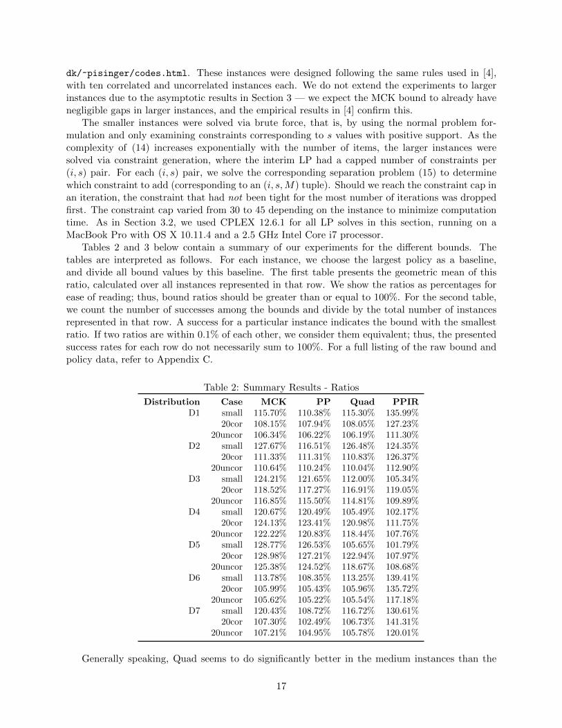
Tables 2 and 3 below contain a summary of our experiments for the different bounds. Thetables are interpreted as follows. For each instance, we choose the largest policy as a baseline,and divide all bound values by this baseline. The first table presents the geometric mean of thisratio, calculated over all instances represented in that row. We show the ratios as percentages forease of reading; thus, bound ratios should be greater than or equal to 100%. For the second table,we count the number of successes among the bounds and divide by the total number of instancesrepresented in that row. A success for a particular instance indicates the bound with the smallestratio. If two ratios are within 0.1% of each other, we consider them equivalent; thus, the presentedsuccess rates for each row do not necessarily sum to 100%. For a full listing of the raw bound andpolicy data, refer to Appendix C.

Table 2: Summary Results - Ratios

Distribution Case MCK PP Quad PPIRD1 small 115.70% 110.38% 115.30% 135.99%

20cor 108.15% 107.94% 108.05% 127.23%20uncor 106.34% 106.22% 106.19% 111.30%

D2 small 127.67% 116.51% 126.48% 124.35%20cor 111.33% 111.31% 110.83% 126.37%

20uncor 110.64% 110.24% 110.04% 112.90%D3 small 124.21% 121.65% 112.00% 105.34%

20cor 118.52% 117.27% 116.91% 119.05%20uncor 116.85% 115.50% 114.81% 109.89%

D4 small 120.67% 120.49% 105.49% 102.17%20cor 124.13% 123.41% 120.98% 111.75%

20uncor 122.22% 120.83% 118.44% 107.76%D5 small 128.77% 126.53% 105.65% 101.79%

20cor 128.98% 127.21% 122.94% 107.97%20uncor 125.38% 124.52% 118.67% 108.68%

D6 small 113.78% 108.35% 113.25% 139.41%20cor 105.99% 105.43% 105.96% 135.72%

20uncor 105.62% 105.22% 105.54% 117.18%D7 small 120.43% 108.72% 116.72% 130.61%

20cor 107.30% 102.49% 106.73% 141.31%20uncor 107.21% 104.95% 105.78% 120.01%

Generally speaking, Quad seems to do significantly better in the medium instances than the

17

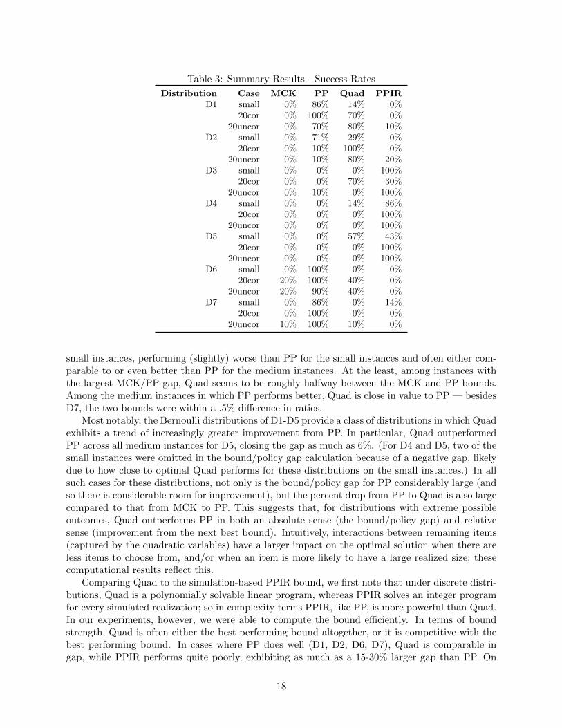
Table 3: Summary Results - Success Rates

Distribution Case MCK PP Quad PPIRD1 small 0% 86% 14% 0%

20cor 0% 100% 70% 0%20uncor 0% 70% 80% 10%

D2 small 0% 71% 29% 0%20cor 0% 10% 100% 0%

20uncor 0% 10% 80% 20%D3 small 0% 0% 0% 100%

20cor 0% 0% 70% 30%20uncor 0% 10% 0% 100%

D4 small 0% 0% 14% 86%20cor 0% 0% 0% 100%

20uncor 0% 0% 0% 100%D5 small 0% 0% 57% 43%

20cor 0% 0% 0% 100%20uncor 0% 0% 0% 100%

D6 small 0% 100% 0% 0%20cor 20% 100% 40% 0%

20uncor 20% 90% 40% 0%D7 small 0% 86% 0% 14%

20cor 0% 100% 0% 0%20uncor 10% 100% 10% 0%

small instances, performing (slightly) worse than PP for the small instances and often either com-parable to or even better than PP for the medium instances. At the least, among instances withthe largest MCK/PP gap, Quad seems to be roughly halfway between the MCK and PP bounds.Among the medium instances in which PP performs better, Quad is close in value to PP — besidesD7, the two bounds were within a .5% difference in ratios.

Most notably, the Bernoulli distributions of D1-D5 provide a class of distributions in which Quadexhibits a trend of increasingly greater improvement from PP. In particular, Quad outperformedPP across all medium instances for D5, closing the gap as much as 6%. (For D4 and D5, two of thesmall instances were omitted in the bound/policy gap calculation because of a negative gap, likelydue to how close to optimal Quad performs for these distributions on the small instances.) In allsuch cases for these distributions, not only is the bound/policy gap for PP considerably large (andso there is considerable room for improvement), but the percent drop from PP to Quad is also largecompared to that from MCK to PP. This suggests that, for distributions with extreme possibleoutcomes, Quad outperforms PP in both an absolute sense (the bound/policy gap) and relativesense (improvement from the next best bound). Intuitively, interactions between remaining items(captured by the quadratic variables) have a larger impact on the optimal solution when there areless items to choose from, and/or when an item is more likely to have a large realized size; thesecomputational results reflect this.

Comparing Quad to the simulation-based PPIR bound, we first note that under discrete distri-butions, Quad is a polynomially solvable linear program, whereas PPIR solves an integer programfor every simulated realization; so in complexity terms PPIR, like PP, is more powerful than Quad.In our experiments, however, we were able to compute the bound efficiently. In terms of boundstrength, Quad is often either the best performing bound altogether, or it is competitive with thebest performing bound. In cases where PP does well (D1, D2, D6, D7), Quad is comparable ingap, while PPIR performs quite poorly, exhibiting as much as a 15-30% larger gap than PP. On

18

the other hand, PPIR tends to perform best under the Bernoulli distributions with the highestvariance (D3, D4, D5); in these cases, Quad is more competitive than PP. Thus, even though itis polynomially solvable, Quad seems to be the most stable bound, compared to the more variedperformances of PP and PPIR.

In general, the gap seems to decrease as the number of items or the number of breakpointsincreases. The trend in the success of Quad versus PP as the number of items increases suggeststhat Quad is better suited for instances with a larger number of items, while PP is better suited forsmaller instances. This is consistent with the notion that Quad is focused more on the combinatorialproperties of the knapsack problem, while PP focuses on the item size to capacity resolution (andis thus better for the small instances, in which each individual item has more influence on theoptimal solution). Coupled with the fact that Quad is polynomially solvable, we conclude that thequadratic bound is a theoretically effective – but characteristically dissimilar – alternative to thepseudo-polynomial bound for (larger) instances in which PP is computationally infeasible. However,since the gap between Quad and the best policy is still not unequivocally tight, the next step wouldbe to find an even better method, ideally an empirically tractable exact algorithm that can helpclose this bound/policy gap.

5 Conclusions

We have studied a dynamic knapsack problem with stochastic item sizes and provided relaxationanalysis on the multiple choice knapsack bound (4). We have shown that the MCK bound isasymptotically optimal as the number of items increases by comparing it to a natural greedy policyand, depending on various growth rates of capacity, delineated reasonable conditions for which theresult holds.

For medium-sized instances with more item-to-capacity granularity, the gap remains a causefor concern, and we proposed a quadratic relaxation whose value function approximation encodesinteractions between item pairs. In addition to showing that it is polynomially solvable and moreefficient than the best known pseudo-polynomial relaxation, our computational experiments indi-cate that the quadratic bound is at least stronger than MCK and faster than PP, while at bestcomparable to or even stronger than PP in both quality and solution time.

The results here contribute to an overall picture of the stochastic knapsack problem that hasyet to be completed. While the asymptotic analysis and quadratic bound impact situations wherethe number of items in the problem are large and medium, respectively, our results demonstratethat even the best performing bounds can empirically have a large gap in certain cases. Thedynamic programming formulation can be directly solved when the number of items is minuscule;otherwise, however, it still remains to develop an empirically efficient algorithm with an optimalityor ε-optimality guarantee. For example, in the spirit of the cutting plane algorithms used in solvingthe deterministic knapsack problem, one could attempt to dynamically improve the value functionapproximation to systematically reach stronger relaxations. However, exactly how a dynamic valuefunction approximation would work for this problem remains an interesting open question.

Acknowledgements

The authors thank Bob Foley and David Goldberg for helpful discussions, as well as the associateeditor and two anonymous referees for the helpful suggestions. D. Blado’s work was partially sup-ported by the National Science Foundation through a Graduate Research Fellowship. A. Toriello’swork was partially supported by the National Science Foundation via grant CMMI-1552479.

19

References

[1] D. Adelman, Price-Directed Replenishment of Subsets: Methodology and its Application toInventory Routing, Manufacturing and Service Operations Management 5 (2003), 348–371.

[2] S.R. Balseiro and D.B. Brown, Approximations to stochastic dynamic programs via informationrelaxation duality, Working paper. Available at http://faculty.fuqua.duke.edu/~dbbrown/bio/papers/balseiro_brown_approximations_16.pdf, 2016.

[3] A. Bhalgat, A. Goel, and S. Khanna, Improved Approximation Results for Stochastic KnapsackProblems, Proceedings of the Twenty-Second Annual ACM-SIAM Symposium on DiscreteAlgorithms, SIAM, 2011, pp. 1647–1665.

[4] D. Blado, W. Hu, and A. Toriello, Semi-Infinite Relaxations for the Dynamic Knapsack Prob-lem with Stochastic Item Sizes, SIAM Journal on Optimization 26 (2016), 1625–1648.

[5] R.L. Carraway, R.L. Schmidt, and L.R. Weatherford, An algorithm for maximizing targetachievement in the stochastic knapsack problem with normal returns, Naval Research Logistics40 (1993), 161–173.

[6] D.P. de Farias and B. van Roy, The Linear Programming Approach to Approximate DynamicProgramming, Operations Research 51 (2003), 850–865.

[7] B.C. Dean, M.X. Goemans, and J. Vondrak, Approximating the Stochastic Knapsack Prob-lem: The Benefit of Adaptivity, Proceedings of the 45th Annual IEEE Symposium on theFoundations of Computer Science, IEEE, 2004, pp. 208–217.

[8] , Adaptivity and Approximation for Stochastic Packing Problems, Proceedings of theSixteenth Annual ACM-SIAM Symposium on Discrete Algorithms, SIAM, 2005, pp. 395–404.

[9] , Approximating the Stochastic Knapsack Problem: The Benefit of Adaptivity, Mathe-matics of Operations Research 33 (2008), 945–964.

[10] C. Derman, G.J. Lieberman, and S.M. Ross, A Renewal Decision Problem, Management Sci-ence 24 (1978), 554–561.

[11] A. Goel and P. Indyk, Stochastic load balancing and related problems, Proceedings of the 40thAnnual IEEE Symposium on the Foundations of Computer Science, IEEE, 1999, pp. 579–586.

[12] V. Goyal and R. Ravi, A PTAS for Chance-Constrained Knapsack Problem with Random ItemSizes, Operations Research Letters 38 (2010), 161–164.

[13] M. Grotschel, L. Lovasz, and A. Schrijver, Geometric Algorithms and Combinatorial Opti-mization, Springer-Verlag, Berlin, 1993.

[14] A. Gupta, R. Krishnaswamy, M. Molinaro, and R. Ravi, Approximation Algorithms for Cor-related Knapsacks and Non-Martingale Bandits, Proceedings of the 52nd IEEE Annual Sym-posium on Foundations of Computer Science, IEEE, 2011, pp. 827–836.

[15] , Approximation Algorithms for Correlated Knapsacks and Non-Martingale Bandits,Preprint available on-line at arxiv.org/abs/1102.3749, 2011.

[16] M. Henig, Risk criteria in a stochastic knapsack problem, Operations Research 38 (1990),820–825.

20

[17] D.S. Hochbaum, Solving Integer Programs over Monotone Inequalities in Three Variables: AFramework for Half Integrality and Good Approximations, European Journal of OperationalResearch 140 (2002), 291–321.

[18] T. Ilhan, S.M.R. Iravani, and M.S. Daskin, The Adaptive Knapsack Problem with StochasticRewards, Operations Research 59 (2011), 242–248.

[19] H. Kellerer, U. Pferschy, and D. Pisinger, Knapsack Problems, Springer-Verlag, Berlin, 2004.

[20] J. Kleinberg, Y. Rabani, and E. Tardos, Allocating Bandwidth for Bursty Connections, Pro-ceedings of the Twenty-Ninth Annual ACM Symposium on the Theory of Computing, Asso-ciation for Computing Machinery, 1997, pp. 664–673.

[21] , Allocating Bandwidth for Bursty Connections, SIAM Journal on Computing 30 (2000),191–217.

[22] A. Kleywegt and J.D. Papastavrou, The Dynamic and Stochastic Knapsack Problem, Opera-tions Research 46 (1998), 17–35.

[23] , The Dynamic and Stochastic Knapsack Problem with Random Sized Items, OperationsResearch 49 (2001), 26–41.

[24] W. Ma, Improvements and Generalizations of Stochastic Knapsack and Multi-Armed BanditAlgorithms, Proceedings of the Twenty-Fifth Annual ACM-SIAM Symposium on DiscreteAlgorithms (SODA), SIAM, 2014, pp. 1154–1163.

[25] S. Martello and P. Toth, Knapsack Problems: Algorithms and Computer Implementations,John Wiley & Sons, Ltd., Chichester, England, 1990.

[26] Y. Merzifonluoglu, J. Geunes, and H.E. Romeijn, The static stochastic knapsack problem withnormally distributed item sizes, Mathematical Programming 134 (2012), 459–489.

[27] H. Morita, H. Ishii, and T. Nishida, Stochastic linear knapsack programming problem and itsapplications to a portfolio selection problem, European Journal of Operational Research 40(1989), 329–336.

[28] J.D. Papastavrou, S. Rajagopalan, and A. Kleywegt, The Dynamic and Stochastic KnapsackProblem with Deadlines, Management Science 42 (1996), 1706–1718.

[29] A. Schrijver, The traveling salesman problem, Combinatorial Optimization: Polyhedra andEfficiency, vol. B, Springer, Berlin, 2003, pp. 981–1004.

[30] P.J. Schweitzer and A. Seidmann, Generalized Polynomial Approximations in Markovian De-cision Processes, Journal of Mathematical Analysis and Applications 110 (1985), 568–582.

[31] M. Sniedovich, Preference order stochastic knapsack problems: methodological issues, Journalof the Operational Research Society 31 (1980), 1025–1032.

[32] E. Steinberg and M.S. Parks, A preference order dynamic program for a knapsack problem withstochastic rewards, Journal of the Operational Research Society 30 (1979), 141–147.

[33] M.A. Trick and S.E. Zin, Spline Approximations to Value Functions: A Linear ProgrammingApproach, Macroeconomic Dynamics 1 (1997), 255–277.

[34] J. Vondrak, Probabilistic Methods in Combinatorial and Stochastic Optimization, Ph.D. thesis,Massachusetts Institute of Technology, 2005.

21

Appendix A - Proof of Theorem 3.11

Proof. It suffices to show that the limit of the ratio is lower bounded by a quantity that goes to 1.Prior to examining each case individually, we observe that under k items, the capacity is

b(k) =∑i≤f(k)

Ei = E[Sf(k)] = Θ(f(k)),

where the linear case sets f(k) = k. With this in mind, the linear case reduces to the case whereb(k) =

∑i≤k Ei = E[Sk], the same as in Lemma 3.6. Since we now limit the number of items to k

(as opposed to an infinite sequence of items), the bounds

Greedy(k, b(k)) ≥∑i≥k

ciP(Si ≤ b(k)), and MCK(k, b(k)) ≤∑i≤k

ciP(Ai ≤ b(k)),

now trivially hold. The Greedy upper bound actually holds at equality by definition of the policy,while the MCK upper bound follows from the (possibly infeasible) solution xi,b(k) = 1 for all i.(This takes advantage of the monotonicity of CDFs, and the fact that there are only at most kitems in the objective.) Thus we have

limk→∞

Greedy(k, b(k))

MCK(k, b(k))≥ lim

k→∞

∑i≤k ciP(Si ≤ E[Sk])∑i≤k ciP(Ai ≤ E[Sk])

= 1,

where the last inequality follows from Lemma 3.6, setting constant c0 to 0. (This shows that themain difficulty for the first regime is finding an additional constant c0 to deal with items i > k.)

For the superlinear case, we have f(k) ≥ k for large enough k, and so

P(Si > b(k)) = P(Si > E[Sf(k)]) ≤ P(Si > E[Sk]).

Therefore,

Greedy(k, b(k))

MCK(k, b(k))=

Greedy(k,E[Sf(k)])

MCK(k,E[Sf(k)])≥∑

i≤k ciP(Si ≤ E[Sf(k)])∑i≤k ciP(Ai ≤ E[Sf(k)])

≥∑

i≤k ciP(Si ≤ E[Sk])∑i≤k ci

≥∑

i≤k ci −O(√k)∑

i≤k ci,

where the last inequality follows from the same calculations as in Lemma 3.6. Because this boundholds for all k, this yields

limk→∞

Greedy(k, b(k))

MCK(k, b(k))≥ lim

k→∞

∑i≤k ci −O(

√k)∑

i≤k ci= 1.

Lastly, for the sublinear case, we have f(k) ≤ k. Recalling that the k items are assumed to begreedily ordered, we have the trivial lower bound

Greedy(k, b(k)) ≥ Greedy(f(k), b(k)) =∑i≤f(k)

ciP(Si ≤ E[Sf(k)]).

22

In the same vein as in Lemma 3.5, then, consider the following solution to the MCK dual problem(4):

q =cf(k)

Ef(k), ri =

ci −

cf(k)Ef(k)

i < f(k)

0 i ≥ f(k), r0(k) = r sup

s∈[0,∞)i=1,2,...,k

[E[Ai|Ai > s]− s

].

Following similar reasoning as in the proof of Lemma 3.5, it is clear the above is a feasible solutionto (4) — simply replace every instance of k in the proof calculations with f(k). The only slightdifference is that the supremum in r0 need only hold for i up to k (as opposed to infinitely manyitems). Assumption (12) in the hypothesis ensures that this quantity is asymptotically dominatedby the other terms. Thus, by setting c0(k) := r0(k)+ rM3/m2, this feasible solution yields objective∑

i≤f(k) ciP(Ai ≤ E[Sf(k)]) + c0(k), providing us with the valid upper bound

MCK(k, b(k)) ≤∑i≤f(k)

ciP(Ai ≤ E[Sf(k)]) + c0(k),

where term c0(k) = o(f(k)).It hence remains to show that

limk→∞

∑i≤f(k) ciP(Si ≤ E[Sf(k)])∑

i≤f(k) ciP(Ai ≤ E[Sf(k)]) + c0(k)≥ lim

k→∞

∑i≤f(k) ciP(Si ≤ E[Sf(k)])∑

i≤f(k) ci + c0(k)= 1.

To this end, we examine

P(Si > E[Sf(k)]) = P(Si − E[Si] > E[Sf(k) − Si]) ≤ P(|Si − E[Si]| > E[Sf(k) − Si])

≤ Var(Si)

(E[Sf(k) − Si])2≤ iV

(f(k)− i)2¯µ2,

noting that E[Sf(k) − Si] ≥ 0 for i ≤ f(k), and the second inequality uses Chebyshev’s bound.Let j be some number such that j < f(k), to be determined, and define upper bound

ci ≤c1E1

Ei ≤ rµ =: c

We now observe∑i≤f(k)

ciP(Si ≤ E[Sf(k)]) =∑i≤j

ciP(Si ≤ E[Sf(k)]) +∑

j<i≤f(k)

ciP(Si ≤ E[Sf(k)])

≥∑i≤j

ci

[1− iV

(f(k)− i)2¯µ2

]+

∑j<i≤f(k)

ci(1− P(Si > E[Sf(k)]))

≥∑i≤f(k)

ci −cV

¯µ2

∑i≤j

i

(f(k)− i)2− c(f(k)− j) ≥

∑i≤f(k)

ci −cV

¯µ2

j+1∫0

x

(f(k)− x)2dx− c(f(k)− j)

=∑i≤f(k)

ci −cV

¯µ2

[ j + 1

f(k)− j − 1+ ln(f(k)− j − 1)− ln f(k)

]− c(f(k)− j),

with the technical condition that f(k) 6∈ [0, j + 1] so that the integrand above does not contain asingularity. Noting that choosing j = f(k)−f(

√k)−1 satisfies this (as identically having f(

√k) = 0

reduces to a trivial case), we have

23

∑i≤f(k)

ciP(Si ≤ E[Sf(k)]) ≥∑i≤f(k)

ci −cV

¯µ2

[f(k)− f(√k)

f(√k)

+ ln f(√k)− ln f(k)

]− c(f(

√k) + 1)

=∑i≤f(k)

ci +O(ln f(k))−O(max f(k)

f(√k), f(√k)).

Therefore, recalling our initial assumptions on∑

i≤f(k) ci and ln f(k), we have

limk→∞

∑i≤f(k) ci +O(ln f(k))−O(max f(k)

f(√k), f(√k))∑

i≤f(k) ci + c0(k)= 1.

The above limit is a valid lower bound for limk→∞Greedy(k,f(k))MCK(k,f(k)) , completing the proof.

Appendix B - MCK for Power Law Distributions

We first recall the following result from [4]:

Proposition. For each i ∈ N , within a segment (s, s) ⊆ [0, b] where Fi is concave and differentiable,the separation problem of MCK (4) can be solved by evaluating s, s and all solutions to

(r0 + ci)d

dsFi(s) = qFi(s) s ∈ (s, s). (16)

It is easy to verify that the power law distributions F1i ,F2i , and F3i in Section 3.2 are concave

and differentiable on [0,∞). Further, (16) has a unique solution for each distribution,

s1i :=r0 + ciq− ai, s2i :=

2(r0 + ci)

q− ai, s3i :=

3(r0 + ci)

q− 2ai,

where s1i , s2i , and s3i correspond to F1i , F

2i and F3i , respectively.

For simplicity, fix a particular distribution j ∈ 1, 2, 3. We implement the following cuttingplane algorithm. Since the constraints in (4) corresponding to s = 0 reduce to non-negativityconstraints, we first solve a relaxation of the MCK bound with only the inequality correspondingto s = b for each i ∈ N . Given a candidate solution (q, r), we check for each i ∈ N if the constraintfor s = sji is satisfied. If any constraints are violated, we add them and re-solve the updated MCKrelaxation to obtain a new candidate solution; otherwise, (q, r) is optimal.

Appendix C - Tables

The following tables present the raw data used to calculate the summary tables presented earlier.The first two tables are used to calculate Table 1, sorting instances by the number of items andvalue/size correlation. Afterward, the next three tables present the raw data used to calculate thesummaries in Tables 2 and 3. These three tables separate instances by their size: small instances,followed by 20-item instances with correlated values-to-sizes under discrete distributions, then 20-item instances with uncorrelated values-to-sizes under discrete distributions.

24

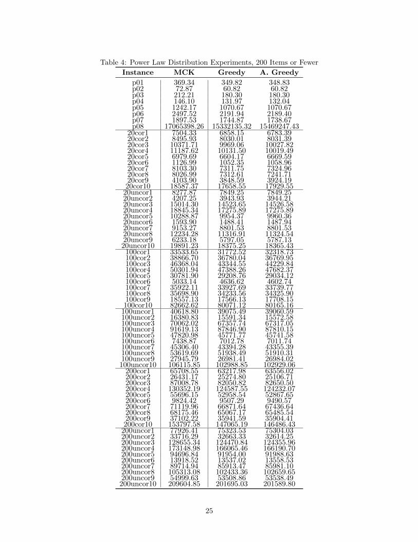
Table 4: Power Law Distribution Experiments, 200 Items or Fewer

Instance MCK Greedy A. Greedy

p01 369.34 349.82 348.83p02 72.87 60.82 60.82p03 212.21 180.30 180.30p04 146.10 131.97 132.04p05 1242.17 1070.67 1070.67p06 2497.52 2191.94 2189.40p07 1897.53 1744.87 1738.67p08 17065398.26 15332135.32 15469247.43

20cor1 7504.33 6858.15 6783.3920cor2 8495.93 8030.01 8031.3920cor3 10371.71 9969.06 10027.8220cor4 11187.62 10131.50 10019.4920cor5 6979.69 6604.17 6669.5920cor6 1126.99 1052.35 1058.9620cor7 8103.30 7311.75 7324.9620cor8 8026.99 7312.61 7241.7120cor9 4103.90 3848.59 3924.1920cor10 18587.37 17658.55 17929.55

20uncor1 8277.87 7849.25 7849.2520uncor2 4207.25 3943.93 3944.2120uncor3 15014.30 14523.65 14526.5820uncor4 18845.34 17275.89 17275.8920uncor5 10288.87 9954.37 9960.3620uncor6 1593.90 1488.41 1487.9420uncor7 9153.27 8801.53 8801.5320uncor8 12234.28 11316.91 11324.5420uncor9 6233.18 5797.05 5787.1320uncor10 19891.23 18375.25 18365.43100cor1 33533.65 31772.52 32318.73100cor2 38866.70 36780.04 36769.95100cor3 46368.04 43344.55 44229.84100cor4 50301.94 47388.26 47682.37100cor5 30781.90 29208.76 29034.12100cor6 5033.14 4636.62 4602.74100cor7 35922.11 33927.69 33739.77100cor8 35698.90 34233.56 34325.90100cor9 18557.13 17566.13 17708.15100cor10 82662.62 80071.12 80165.16

100uncor1 40618.80 39075.49 39060.59100uncor2 16380.83 15591.34 15572.58100uncor3 70062.02 67357.74 67317.05100uncor4 91619.13 87846.90 87810.15100uncor5 47820.98 45771.77 45741.58100uncor6 7438.87 7012.78 7011.74100uncor7 45306.40 43394.28 43355.39100uncor8 53619.69 51938.49 51910.31100uncor9 27945.79 26981.41 26984.02100uncor10 106115.85 102988.85 102929.06

200cor1 65708.55 63217.98 63556.02200cor2 26431.17 25274.80 25106.71200cor3 87008.78 82050.82 82650.50200cor4 130352.19 124587.55 124232.07200cor5 55696.15 52958.54 52867.65200cor6 9824.42 9507.29 9490.57200cor7 71119.96 66871.64 67436.64200cor8 68175.46 65067.17 65485.54200cor9 37102.22 35941.59 35904.41200cor10 153797.58 147065.19 146486.43

200uncor1 77926.41 75323.53 75304.03200uncor2 33716.29 32663.33 32614.25200uncor3 128655.34 124470.84 124355.96200uncor4 173148.98 166065.46 166190.70200uncor5 94696.84 91954.00 91988.63200uncor6 13918.52 13537.02 13558.53200uncor7 89714.94 85913.47 85981.10200uncor8 105313.08 102433.36 102659.65200uncor9 54999.63 53508.86 53538.49200uncor10 209604.85 201695.03 201589.80

25

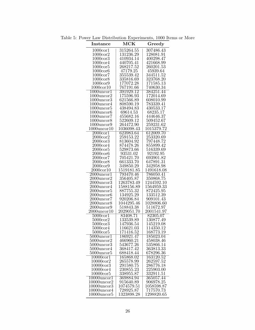
Table 5: Power Law Distribution Experiments, 1000 Items or More

Instance MCK Greedy

1000cor1 315264.55 307486.431000cor2 131236.29 128081.911000cor3 410934.14 400298.471000cor4 440705.41 421668.991000cor5 268217.52 260201.531000cor6 47179.25 45939.641000cor7 355539.42 344511.521000cor8 335816.69 323768.201000cor9 177072.28 171585.131000cor10 767191.66 740630.34

1000uncor1 391929.12 384251.441000uncor2 175596.93 172014.691000uncor3 621566.89 608010.991000uncor4 808590.19 783339.411000uncor5 438494.83 430533.171000uncor6 69614.53 68235.171000uncor7 455682.16 444646.371000uncor8 522609.12 509452.671000uncor9 264472.90 259231.621000uncor10 1036098.43 1015379.72

2000cor1 623983.64 612009.702000cor2 259153.22 253320.692000cor3 813604.92 797448.722000cor4 874478.26 855899.422000cor5 529873.66 516339.692000cor6 93531.02 92192.952000cor7 705421.70 693901.822000cor8 661333.70 647891.312000cor9 349850.29 342958.982000cor10 1519181.85 1491618.08

2000uncor1 793470.46 786050.412000uncor2 356405.87 350868.752000uncor3 1263783.49 1244592.102000uncor4 1588156.89 1564959.332000uncor5 887755.32 872425.952000uncor6 134925.29 133512.392000uncor7 920206.84 909101.432000uncor8 1044295.46 1028806.602000uncor9 518843.38 511672.972000uncor10 2029051.70 2001541.97

5000cor1 83408.71 82305.075000cor2 133539.89 130877.495000cor3 147936.54 145219.085000cor4 116621.03 114350.125000cor5 171416.52 168773.19

5000uncor1 186921.47 185023.045000uncor2 466960.21 458038.465000uncor3 543677.26 535866.145000uncor4 368417.42 363813.335000uncor5 688418.44 678296.3610000cor1 165868.02 163120.5210000cor2 265578.99 262597.5210000cor3 291580.75 286776.1810000cor4 230855.23 225903.0010000cor5 338955.87 332911.51

10000uncor1 369884.94 365057.4410000uncor2 915640.89 906978.2510000uncor3 1074579.51 1058598.8710000uncor4 728925.87 717570.7310000uncor5 1323898.28 1298820.65

26

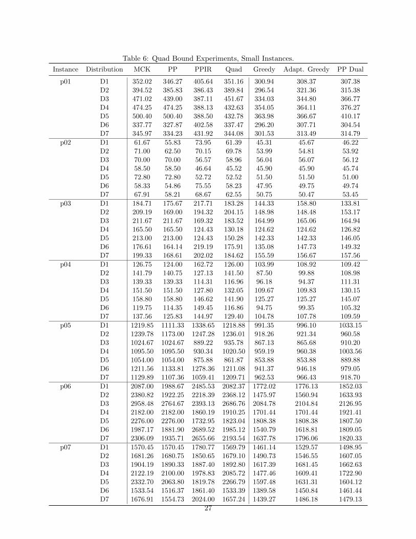
Table 6: Quad Bound Experiments, Small Instances.

Instance Distribution MCK PP PPIR Quad Greedy Adapt. Greedy PP Dual

p01 D1 352.02 346.27 405.64 351.16 300.94 308.37 307.38D2 394.52 385.83 386.43 389.84 296.54 321.36 315.38D3 471.02 439.00 387.11 451.67 334.03 344.80 366.77D4 474.25 474.25 388.13 432.63 354.05 364.11 376.27D5 500.40 500.40 388.50 432.78 363.98 366.67 410.17D6 337.77 327.87 402.58 337.47 296.20 307.71 304.54D7 345.97 334.23 431.92 344.08 301.53 313.49 314.79

p02 D1 61.67 55.83 73.95 61.39 45.31 45.67 46.22D2 71.00 62.50 70.15 69.78 53.99 54.81 53.92D3 70.00 70.00 56.57 58.96 56.04 56.07 56.12D4 58.50 58.50 46.64 45.52 45.90 45.90 45.74D5 72.80 72.80 52.72 52.52 51.50 51.50 51.00D6 58.33 54.86 75.55 58.23 47.95 49.75 49.74D7 67.91 58.21 68.67 62.55 50.75 50.47 53.45

p03 D1 184.71 175.67 217.71 183.28 144.33 158.80 133.81D2 209.19 169.00 194.32 204.15 148.98 148.48 153.17D3 211.67 211.67 169.32 183.52 164.99 165.06 164.94D4 165.50 165.50 124.43 130.18 124.62 124.62 126.82D5 213.00 213.00 124.43 150.28 142.33 142.33 146.05D6 176.61 164.14 219.19 175.91 135.08 147.73 149.32D7 199.33 168.61 202.02 184.62 155.59 156.67 157.56

p04 D1 126.75 124.00 162.72 126.00 103.99 108.92 109.42D2 141.79 140.75 127.13 141.50 87.50 99.88 108.98D3 139.33 139.33 114.31 116.96 96.18 94.37 111.31D4 151.50 151.50 127.80 132.05 109.67 109.83 130.15D5 158.80 158.80 146.62 141.90 125.27 125.27 145.07D6 119.75 114.35 149.45 116.86 94.75 99.35 105.32D7 137.56 125.83 144.97 129.40 104.78 107.78 109.59

p05 D1 1219.85 1111.33 1338.65 1218.88 991.35 996.10 1033.15D2 1239.78 1173.00 1247.28 1236.01 918.26 921.34 960.58D3 1024.67 1024.67 889.22 935.78 867.13 865.68 910.20D4 1095.50 1095.50 930.34 1020.50 959.19 960.38 1003.56D5 1054.00 1054.00 875.88 861.87 853.88 853.88 889.88D6 1211.56 1133.81 1278.36 1211.08 941.37 946.18 979.05D7 1129.89 1107.36 1059.41 1209.71 962.53 966.43 918.70

p06 D1 2087.00 1988.67 2485.53 2082.37 1772.02 1776.13 1852.03D2 2380.82 1922.25 2218.39 2368.12 1475.97 1560.94 1633.93D3 2958.48 2764.67 2393.13 2686.76 2084.78 2104.84 2126.95D4 2182.00 2182.00 1860.19 1910.25 1701.44 1701.44 1921.41D5 2276.00 2276.00 1732.95 1823.04 1808.38 1808.38 1807.50D6 1987.17 1881.90 2689.52 1985.12 1540.79 1618.81 1809.05D7 2306.09 1935.71 2655.66 2193.54 1637.78 1796.06 1820.33

p07 D1 1570.45 1570.45 1780.77 1569.79 1461.14 1529.57 1498.95D2 1681.26 1680.75 1850.65 1679.10 1490.73 1546.55 1607.05D3 1904.19 1890.33 1887.40 1892.80 1617.39 1681.45 1662.63D4 2122.19 2100.00 1978.83 2085.72 1477.46 1609.41 1722.90D5 2332.70 2063.80 1819.78 2266.79 1597.48 1631.31 1604.12D6 1533.54 1516.37 1861.40 1533.39 1389.58 1450.84 1461.44D7 1676.91 1554.73 2024.00 1657.24 1439.27 1486.18 1479.13

27

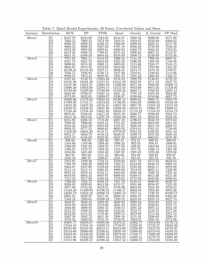
Table 7: Quad Bound Experiments, 20 Items, Correlated Values and Sizes.

Instance Distribution MCK PP PPIR Quad Greedy A. Greedy PP Dual

20cor1 D1 6547.70 6534.08 7482.03 6544.87 5938.42 6099.08 6171.09D2 7062.53 7062.53 7874.59 7043.21 5924.07 6222.89 6286.62D3 8060.70 8006.22 8230.19 7968.06 6209.93 6622.21 6717.28D4 9008.53 9008.53 8347.92 8797.18 6568.58 6758.89 7049.40D5 9872.03 9805.00 8393.61 9480.92 6460.73 6682.43 7253.35D6 6373.28 6366.73 7790.07 6372.43 5806.62 6067.55 6113.27D7 6851.31 6488.59 6804.82 8534.09 5908.74 6249.09 6173.48

20cor2 D1 7971.85 7961.11 8518.85 7966.16 7141.35 7308.58 6997.31D2 8351.73 8351.73 8652.96 8325.22 7296.38 7408.28 7188.36D3 9009.65 8974.28 8908.13 8883.68 7415.06 7594.17 7516.15D4 9602.87 9572.50 8472.94 9310.09 7522.97 7782.96 7455.27D5 10139.45 10116.92 8767.71 9636.28 7674.77 7879.19 7759.27D6 7830.75 7826.85 8746.74 7827.80 7210.61 7188.83 7114.96D7 8092.27 7912.47 9282.23 7931.27 7305.33 7308.93 7432.47

20cor3 D1 9167.63 9149.73 11004.46 9158.33 7898.79 8146.01 8170.18D2 10191.30 10191.30 11817.91 10141.93 8043.78 8711.34 9247.72D3 12137.80 12055.31 12962.33 11999.00 8971.92 9594.06 10268.15D4 13998.30 13833.00 12794.14 13722.50 9503.80 9873.56 11328.91D5 15792.60 15588.80 12769.80 15229.32 9888.71 9768.93 12051.51D6 8824.38 8798.57 11687.14 8821.12 7705.19 8478.39 8663.99D7 9573.95 9022.65 13369.87 9536.87 8198.66 8534.60 8697.73

20cor4 D1 10200.86 10179.83 13043.34 10196.21 8098.62 8666.75 9203.79D2 11760.36 11741.71 14253.92 11726.95 8565.03 10066.95 10104.68D3 14818.20 14437.33 13516.45 14627.58 9887.58 11047.59 12575.56D4 16348.50 16348.50 13881.98 15889.58 10618.45 10363.27 13009.51D5 17548.40 17548.40 15631.80 16634.45 11119.24 11104.42 14744.74D6 9673.61 9520.03 14217.35 9672.23 8086.77 8599.69 8585.73D7 10311.55 9854.05 14797.58 10291.88 8891.16 9659.94 9588.59

20cor5 D1 6315.83 6303.58 7719.30 6307.18 5196.81 5633.79 5973.04D2 7096.00 7096.00 8322.12 7051.67 5560.68 6004.09 6281.05D3 8543.33 8445.39 8565.03 8435.97 5946.88 6651.50 6808.53D4 9938.25 9777.25 8600.85 9693.92 6764.61 6761.31 7738.69D5 11250.80 10944.30 9118.71 10758.67 6764.45 6492.35 8851.44D6 6052.17 6003.79 8159.53 6049.07 5299.73 5657.62 5695.33D7 6352.19 6138.62 9022.90 6347.28 5609.18 6062.61 6078.36

20cor6 D1 998.89 996.92 1269.46 997.45 872.51 899.58 899.92D2 1104.06 1104.06 1269.46 1096.32 892.04 956.31 1008.61D3 1299.39 1291.50 1359.22 1277.95 939.93 1004.98 1104.02D4 1480.81 1475.75 1359.42 1441.68 970.79 1086.13 1201.09D5 1653.66 1621.60 1358.33 1587.92 1091.82 1070.46 1279.56D6 963.56 961.08 1241.42 963.06 884.08 929.92 932.67D7 1034.44 980.37 1400.67 1031.17 887.65 927.52 945.48

20cor7 D1 7053.95 7039.38 7732.74 7050.94 6357.79 6577.62 6622.64D2 7480.29 7480.29 8003.99 7463.71 6544.66 6848.10 6902.24D3 8304.81 8247.00 8193.68 8249.22 6769.86 6823.11 6894.86D4 9115.14 9115.14 8226.35 8909.89 7012.93 6955.11 7229.98D5 9876.44 9876.44 8544.11 9464.60 6888.49 7026.79 7455.42D6 6910.95 6904.42 8035.97 6909.94 6489.57 6614.30 6521.30D7 7312.33 7017.08 8448.43 7278.05 6757.69 6835.66 6886.63

20cor8 D1 7296.63 7282.72 8939.19 7287.19 6138.55 6690.95 6839.47D2 8209.63 8209.63 9613.26 8152.57 6501.86 6858.07 7225.20D3 9977.80 9742.28 9519.25 9748.99 6634.92 7654.29 8558.24D4 11544.38 11439.69 10196.18 11166.77 8063.33 7958.40 9802.36D5 13056.73 12622.10 10686.75 12305.75 7957.51 7720.70 10160.77D6 6991.55 6889.97 9417.43 6988.52 6088.47 6326.56 6404.30D7 7343.18 7080.65 10206.42 7329.18 6322.24 6924.74 6827.74

20cor9 D1 3643.67 3636.42 4382.46 3640.93 3092.34 3210.85 3225.14D2 4050.00 4050.00 4710.08 4031.84 3291.87 3592.65 3537.75D3 4846.00 4809.83 5204.72 4760.54 3491.23 3687.15 4041.59D4 5574.25 5509.25 5024.08 5423.81 3753.73 4153.73 4577.26D5 6272.00 6155.50 5176.30 5999.72 3679.98 3715.32 4937.54D6 3507.33 3502.72 4621.36 3506.50 3121.35 3298.69 3296.45D7 3776.45 3568.20 5252.18 3759.85 3263.37 3505.23 3573.86

20cor10 D1 16391.77 16359.07 18868.03 16379.27 14302.77 14553.03 15176.72D2 17818.10 17818.10 19839.74 17750.67 15328.02 15732.37 16010.08D3 20555.60 20424.80 20613.51 20352.69 15226.99 15847.02 16770.37D4 23124.60 23060.00 22326.61 22695.50 17066.65 16519.04 18556.25D5 25642.00 25230.50 21020.76 23979.03 17100.77 17696.29 19030.89D6 15914.68 15832.62 19805.42 15910.38 14330.15 14779.72 15087.60D7 17151.96 16228.57 21888.46 17057.42 15066.57 15724.06 15785.30

28

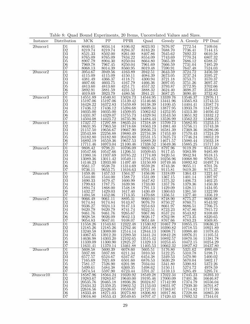
Table 8: Quad Bound Experiments, 20 Items, Uncorrelated Values and Sizes.

Instance Distribution MCK PP PPIR Quad Greedy A. Greedy PP Dual

20uncor1 D1 8040.61 8034.14 8106.02 8023.93 7676.97 7772.54 7109.04D2 8219.74 8219.74 8294.37 8183.20 7688.70 7736.41 7144.15D3 8521.33 8502.00 8261.00 8407.86 7645.62 7692.22 6610.58D4 8765.09 8765.09 7834.22 8554.09 7743.69 7770.24 6807.32D5 8907.79 8904.30 8250.04 8664.80 7665.39 7686.12 6588.37D6 7969.78 7967.45 8250.04 7961.69 7666.59 7731.04 7485.29D7 8068.13 8014.39 8560.95 8019.48 7590.91 7647.48 7524.03

20uncor2 D1 3954.67 3949.56 4163.89 3942.51 3643.59 3724.72 3456.59D2 4115.09 4115.09 4150.11 4084.39 3673.05 3737.24 3595.27D3 4381.49 4366.37 4118.71 4300.94 3721.18 3753.71 3570.37D4 4607.66 4603.75 4167.79 4466.36 3697.05 3751.26 3697.37D5 4813.60 4813.60 4251.71 4557.32 3793.87 3772.95 3702.66D6 3892.91 3881.59 4231.52 3888.32 3624.40 3698.27 3538.63D7 4019.69 3923.79 4480.56 3941.21 3687.25 3690.40 3732.82

20uncor3 D1 14551.89 14540.81 15024.73 14544.95 13339.76 13546.37 12976.11D2 15197.06 15197.06 15139.42 15146.66 13441.96 13565.83 12743.55D3 16428.22 16372.83 15459.89 16138.39 14100.45 14404.41 13587.74D4 17436.12 17436.12 15394.68 16699.34 13877.95 13933.78 13472.95D5 16035.00 16035.00 14509.05 15062.62 14252.95 14313.30 14056.42D6 14331.97 14329.07 15755.73 14329.94 13543.50 13651.92 13332.12D7 14504.08 14423.72 16735.96 14484.43 13526.99 13562.22 13468.22

20uncor4 D1 17327.77 17297.88 18635.24 17318.48 15709.73 15682.95 15253.15D2 18631.95 17963.50 18718.68 18563.19 14981.40 15756.11 15743.38D3 21157.50 19656.67 19667.90 20836.73 16581.39 17369.36 16286.06D4 23543.88 22256.88 19880.49 22734.38 17453.40 17570.43 17224.29D5 24182.80 24182.80 20423.80 22531.15 17625.73 17746.24 18052.19D6 16892.19 16559.36 19657.53 16889.20 14671.57 15080.44 15033.18D7 17711.46 16973.04 21100.46 17338.52 15649.36 15885.25 15717.10

20uncor5 D1 9808.42 9798.21 10706.09 9802.68 8797.96 9119.29 8513.68D2 10547.66 10547.66 11206.51 10509.65 9117.45 9383.99 9485.89D3 11980.16 11937.69 10785.22 11774.89 9420.54 9942.94 9518.15D4 13089.36 13011.42 10549.11 12791.65 10256.96 10068.90 9769.55D5 14146.23 13933.00 11497.40 13150.89 10749.46 10892.82 10497.74D6 9561.17 9538.70 11314.69 9559.28 8743.38 9055.11 8701.76D7 9736.11 9653.75 11616.63 9701.18 9115.81 9419.20 9175.37

20uncor6 D1 1459.46 1457.53 1564.37 1456.06 1318.09 1364.43 1221.44D2 1544.00 1544.00 1588.72 1531.09 1367.15 1401.14 1397.97D3 1690.33 1679.47 1600.99 1647.82 1375.32 1406.73 1402.25D4 1799.63 1787.75 1639.98 1733.00 1357.76 1379.36 1450.30D5 1894.74 1868.00 1548.18 1791.13 1429.09 1428.11 1434.95D6 1432.27 1429.03 1617.40 1430.49 1360.63 1381.50 1322.99D7 1494.58 1452.06 1713.35 1470.68 1356.51 1377.40 1356.19

20uncor7 D1 9066.49 9061.11 8895.31 9060.04 8748.90 8775.27 8606.08D2 9174.84 9174.84 9143.87 9076.70 8750.27 8760.71 8543.92D3 9336.27 9324.13 9147.13 9254.63 8661.97 8686.51 7766.75D4 9420.79 9420.79 8741.74 9322.51 8723.23 8747.86 7915.72D5 9461.76 9461.76 9265.67 9367.86 8537.24 8543.82 8108.69D6 9028.58 9026.09 9042.13 9026.17 8762.98 8773.35 8320.65D7 9054.83 9047.01 9108.07 9051.68 8767.66 8783.23 8569.85

20uncor8 D1 11558.26 11543.61 12322.48 11530.82 10467.79 10855.15 10636.21D2 12185.26 12185.26 12762.46 12051.89 10390.82 10718.55 10921.89D3 13240.58 13089.00 12514.14 12844.13 10698.71 10988.40 11078.45D4 14067.65 13912.20 12289.50 13441.24 10842.28 10976.21 11105.51D5 14636.98 14303.20 12102.65 13515.42 10892.57 10870.16 11381.78D6 11339.09 11300.90 12825.27 11329.13 10253.45 10472.15 10254.29D7 11631.41 11370.14 13461.88 11405.53 10662.32 10827.82 10437.80

20uncor9 D1 5608.58 5600.39 6078.60 5605.51 5176.80 5321.62 4995.69D2 5937.88 5937.88 6211.34 5910.50 5122.25 5310.78 5198.71D3 6577.57 6524.67 6347.67 6454.38 5349.53 5470.90 5400.02D4 7165.69 7021.69 6501.60 6876.53 5630.29 5670.04 5802.17D5 7581.17 7526.90 6201.98 7034.04 5341.80 5390.83 5372.26D6 5499.61 5484.38 6369.35 5498.62 5150.11 5274.72 4978.59D7 5874.54 5597.90 6723.44 5701.37 5159.13 5285.49 5295.74

20uncor10 D1 18587.96 18564.24 19320.92 18549.28 17022.34 17445.23 16393.10D2 19283.67 19283.67 19640.00 19195.46 17000.09 17401.36 16646.87D3 20535.76 20465.18 18936.26 20324.87 17142.99 17374.79 16556.04D4 21634.32 21359.25 19802.52 21153.03 18031.97 17939.30 16701.87D5 22616.56 22426.05 19559.67 21727.01 17383.87 17714.82 17177.66D6 18333.48 18271.03 20273.80 18306.80 16917.86 17228.88 16865.20D7 19016.80 18553.43 20549.65 18707.47 17420.43 17692.52 17344.01

29