The accounting choice issue and the M&A activity

Humberto Ribeiro*

Draft paper. Please do not quote or distribute without the permission of the author

* De Montfort University, Leicester, UK. Correspondence address: Leicester Business School, The Gateway, Leicester LE1 9BH, UK. Phone +447981924726. E-mail: hn2rpt@gmail.com.

The accounting choice issue and the M&A activity

Abstract - This study addresses the issue of the accounting choice as a possible determinant of mergers & acquisitions (M&A) activity. The accounting choice has value implications, and managerial discretion can be used to meet financial reporting objectives (see e.g. Watts & Zimmerman, 1990). On the other hand, despite the existence of a wide empirical and theoretical research, the literature still lacks a convincing overall theory concerning M&A occurrence. Nevertheless, the overall evidence suggests that some macroeconomic variables are associated with the timing of M&A. This paper studies whether accounting choice developments can affect M&A activity together with macroeconomic, time, and several M&A endogenous variables. The findings show a significant positive relationship between M&A activity and stock market prices, and also several significant associations between M&A and other endogenous and exogenous explanatory variables, but no relationship between accounting choice and M&A activity. EFM classification: 710, 160, 200 Keywords: Mergers, Acquisitions, Business combinations, Time series, U.S.A.

2

1. Introduction Usually managers have discretion in the application of the generally accepted

accounting principles (GAAP). The set of accounting procedures within which

managers have discretion is commonly known as the "accepted set." (Watts &

Zimmerman, 1990). According these authors, the managerial discretion over the

accounting method choice is expected to vary across firms with the variation in the

costs and benefits of restrictions (enforced by external auditors) which will produce the

"best" or "accepted" accounting principles. The managerial discretion can be used to

meet financial reporting objectives. Moreover, the achievement of objectives benefits

managers whose compensation is tied to financial information. Whether shareholders

benefit from managerial discretion and whether the benefits outweigh the costs is not

such a clear matter (Fields et al., 2001).

The accounting choice has value implications. Several studies have found that both

acquirer and target companies select an accounting method based upon certain financial

and non-financial characteristics (Davis, 1990). The percentage of insiders’ ownership,

accounting-based compensation plans, leveraged-based lending agreements, the

company size and some other specific characteristics determine which accounting

method is selected (Dunne, 1990). For instance, managers at companies with

compensations based upon earnings favoured pooling of interest method because it

benefited earnings and return on investment (Aboody et al., 2000; Gagnon, 1967).

Two traditional methods are used to account for business combinations: the purchase

method (purchase) and the pooling of interests method (pooling). The literature focused

on the pooling-purchase choice is relatively large. It may be worth briefly reviewing

some of it. Many studies documented that the short-window announcement returns are

lower for pooling firms than for purchase firms (Davis, 1990; Hong et al., 1978;

Martinez-Jerez, 2001). It has been also found that pooling firms willingly incur

significant costs to achieve the desired financial reporting outcome (Ayers et al., 2002;

Lys & Vincent, 1995; Weber, 2004). Other studies pictured that pooling method results

in mechanical effects on companies’ financial statements and on the analysis of the

financial statements (Jennings et al., 1996; Vincent, 1997).

3

Discussions about business combinations easily generate controversies because they

may lead to dramatic changes to the financial statements. When the prohibition of use of

pooling was discussed in the U.S in late 1990’s, many companies and professional

boards strongly disagreed because they were concerned with managing cash flows over

earnings per share (EPS) and therefore they were afraid of goodwill and amortization

charges. They argued that many M&A deals would not be possible do complete without

pooling (e.g. major deals involving enormous companies with large goodwill and other

intangible assets balances). Therefore, the M&A activity and the economy could suffer

from this potential constraint.

Pooling worked has an accounting option and that was an advantage for certain

companies and some sectors. It represented also an opportunity for creative accounting.

However, the pooling benefits had inherent some relevant costs. Companies often

consumed “substantial resources” structuring transactions merely to meet the

requirements of pooling (Linsmeier et al., 1998), spending massive fees with legal and

financial advisors. This concern could even lead to put the formal aspects over the

corporate strategy – a mistake at M&A level.

Despite some disagreements, pooling was banned in the U.S.A. - 1 July 2001 - and also

at international level, as the International Accounting Standards Board (IASB) followed

in 2004 the initiative of its American counterpart, the Financial Accounting Standards

Board (FASB). Another innovation brought by FASB and also followed by IASB, was

the replacement of purchased goodwill amortization by impairment tests.

2. The M&A phenomenon Why M&A occurs continues to be a phenomenon not fully understood. Despite all

efforts made, previous researchers have been unable to reach a consensus about the

theoretical framework that underlies M&A activity and its wave pattern.1 In fact,

1 The finding that M&A occurs in waves seems to be indisputable as almost all authors admit it (e.g. Andrade & Stafford, 2004; Barkoulas et al., 2001; Gort, 1969; Harford, 2005; Mitchell & Mulherin, 1996; Nelson, 1959; Rhodes-Kropf et al., 2005; Stigler, 1950; Weston et al., 2004). Only Shughart II & Tollison (1984) were unable to recognize it, generating afterwards replies from Golbe & White (1988) and Town (1992).

4

despite the existence of a wide empirical and theoretical research, the literature still

lacks a convincing overall theory, presenting many partial explanations instead.2

Some literature attempts to explain overall M&A activity using a neoclassical approach

(See e.g. Andrade et al., 2001; Andrade & Stafford, 2004; Gort, 1969; Harford, 2005;

Mitchell & Mulherin, 1996; Sudarsanam, 2003; Weston et al., 2004), arguing that

merger waves result from shocks, such as technological innovations or deregulation, to

an industry’s environment (Harford, 2005), while other authors believe that M&A

waves occur as a result of temporary stock market misevaluation (e.g. Dong et al., 2006;

Rhodes-Kropf et al., 2005; Rhodes-Kropf & Viswanathan, 2004; Shleifer & Vishny,

2003).3 This second approach, commonly labelled behavioural, is built on theoretical

and empirical research which has observed a positive statistically significant correlation

between aggregate share valuations and merger activity (Beckenstein, 1979; Becketti,

1986; Golbe & White, 1988; Guerard, 1985; Markham, 1955; Melicher et al., 1983;

Nelson, 1959; Steiner, 1975; Weston, 1953).4 Beyond the mainstream approaches, there

are also other attempts using other different arguments.5 In terms of the type of data

utilised, several empirical studies have tested the wave pattern using aggregate industry

data (e.g. Barkoulas et al., 2001; Becketti, 1986; Golbe & White, 1993; Melicher et al.,

1983; Mueller, 1980; Town, 1992), while others studied this phenomenon at industry

(e.g. Andrade et al., 2001; Eis, 1969; Gort, 1969; Harford, 2005; Mitchell & Mulherin,

1996), or at institutional levels (e.g. Auster & Sirower, 2002).

The overall evidence suggests that some macroeconomic variables are associated with

the timing of M&A. The activity is procyclical, as generally it leads slightly the

business cycle (see e.g. Golbe & White, 1988; Nelson, 1959; Steiner, 1975; Weston et

al., 1990). According to Weston (1990), the activity is also approximately coincident

with share price movements. Several authors find that share prices lead the M&A

activity (e.g. Nelson, 1959), while others conversely conclude that M&A activity lags

2 e.g. for more than twenty years that Brealey et al. (1984; 1996; 2006) continue to select the occurrence of M&A waves as one of the ten most relevant currently unsolved problems in finance. 3 Market misvaluation can be defined as the discrepancy between the market price and a present measure of the fundamental value (Dong et al., 2006). 4 The wide existent literature is quasi unanimous about it. 5 e.g. Holmstrom & Kaplan (2001) focus on the role of corporate governance in the occurrence of M&A waves.

5

the stock market movements (e.g. Melicher et al., 1983).6 This divergence of findings

may be explained by the time spent between the beginning of the negotiations and the

accomplishment of the deal. Halpern (1973) and Mandelker (1974) find this period to

be on average about six months. Therefore Melicher et al. (1983), who evaluate share

prices changes to precede M&A completed deals by one quarter, conclude that M&A

negotiations lead share price movements by about one quarter.

Another stream of literature has studied the market effects of the existence of two

different accounting methods for business combinations: the purchase method and the

pooling of interests method. Several studies suggest that firms involved in M&A deals

select an accounting method based upon certain financial and non-financial

characteristics (e.g. Davis, 1990; Dunne, 1990). It has also been documented that

managers prefer pooling and that pooling firms willingly incur significant costs to

achieve the desired financial reporting outcome (Aboody et al., 2000; Ayers et al., 2002;

Lys & Vincent, 1995; Robinson & Shane, 1990; Walter, 1999; Weber, 2004). Despite

the preference for pooling however, empirical evidence supports market efficiency,

which means that M&A is valued the same regardless the pooling versus purchase

adoption (e.g. Davis, 1990; Hong et al., 1978; Lindenberg & Ross, 1999; Vincent,

1997).7 Nevertheless, existent literature also revealed that pooling results in mechanical

effects on companies’ financial statements and on the analysis of the financial

statements (Jennings et al., 1996; Vincent, 1997).

The replacement of the purchased goodwill amortization method by impairment tests

may also have an impact on M&A activity. The research findings indicate that the

market reacts negatively to the amortization of goodwill by purchase firms (e.g. Ayers

et al., 2002; Hopkins et al., 2000). Not surprisingly, several authors (e.g. Robinson &

Shane, 1990) find that a higher bid premium, enhancing the size of the potential

goodwill, increases the likelihood of pooling (Weston et al., 2004). Nevertheless, share

prices should not decline significantly for companies with one-time impairment write-

offs, unless they become habitual (Hopkins et al., 2000).

6 According to Mueller (1980), in West Germany, during the 1960s M&A activity lagged share prices. However, in the 1970s M&A activity tended to lead share prices and other aggregate measures, such as GDP and gross fixed investment. 7 Nevertheless, according to Hopkins et al. (2000), analysts’ valuations were lowest when a company adopted purchase method and amortized goodwill.

6

Supported by the empirical findings presented above, the first hypothesis to be tested is

exhibited below in the null form:

Hypothesis 1

The FASB new pronouncements have had no impact on the M&A activity, as its

evolution is rather explained by other factors, such as financial, economical, or

behavioural ones.

The analysis of the results of this first hypothesis provides evidence about any impacts

on the M&A activity from the abolishment of pooling of interests and the replacement

of purchased goodwill amortization by impairment tests. Therefore, this hypothesis tests

the appropriateness of FASB’s new rules, in the scope of the desired neutrality of the

accounting standards. The testing also documents the influence of economical, financial

and time factors to the pattern of M&A occurrence.

The impossibility of rejecting this hypothesis would suggest that M&A activity is

unrelated to FASB changes and is rather driven by financial, economical, time, or other

factors. Conversely, rejection of hypothesis number one would suggest that FASB new

pronouncements had produced a significant impact to M&A market participants and

failed to minimize any possible economic effects. In this case, the other two possible

hypotheses, called alternative hypotheses, are that the M&A activity benefited from the

accounting changes, and that M&A activity did not benefit from the accounting

changes.

3. M&A withdrawal A substantial number of announced M&A deals are never completed. For example,

Pickering (1978) reports a 14 % abandonment rate, while Muehlfeld et al. (2006)

estimates it to be as high as 27 %. In the period in between 2000 and 2002, the rate of

deals announced but not completed in the U.S.A. was 20 %.8 This fact is relevant,

8 Author estimation (source: Thomson Financial, 2006).

7

because M&A can be very expensive, so can its abandonment, since firms need to

allocate significant resources while planning and preparing a deal.

The literature concerned with the study of M&A abandonment causes is scarce. The

majority of the studies focus on the post-M&A period analysis; only a few are

concerned with the analysis of the pre-completion phase and M&A cancellations.9

Muehlfeld et al. (2006) point out a major difficulty related to this type of analysis:

“Decision-making processes at the pre-completion stage are largely unobservable to

financial markets and difficult to capture based on accounting data.” Despite the non-

existence of a global theory, existing literature provides some evidence to help explain

these occurrences. The explaining factors are mainly related with the type and way of

concretization of the M&A deal. Bidder and target firms’ characteristics and attitudes

also play key roles.

Dodd (1980) emphasizes that M&A bids and proposals are subject to discretional

decision from the management. The target firm’s shareholders delegate the decision to

the management, but hold the power to vote after their recommendations have been

made following M&A proposals. Nevertheless, the management has the power to

decline any friendly M&A proposal without presenting it to the shareholders. According

to Davidson III et al. (2002), this power can be regarded as a safeguard to the firm,

insuring that the M&A is adequate (Franks & Mayer, 1996), but conversely it can also

be perceived as an instrument of protection for the management, used with the purpose

of avoiding the loss of their own positions in the target firm as a consequence of a

successful takeover, at shareholders expense (Karpoff et al., 1996). Consequently,

cancelled M&A often reflect an agency theory issue, where the interests of the

management did not coincide with the interests of the shareholders (Davidson III et al.,

2002).

Concerning the bidder’s attitude, Holl & Kyriazis (1996) point out that hostile takeovers

are more likely to meet resistance from target firms. Often negotiations that started

friendly end up in disagreements. This makes transactions more costly and increases the

likelihood of a bid cancellation. If a bid is considered friendly one could expect it to be

9 As exceptions see e.g. Asquith (1983), Wong & O’Sullivan (2001), Davidson III et al. (2002).

8

less dependent upon negotiations to be successful, as it would be less susceptible to face

resistance from the target firms’ management (Wong & O’Sullivan, 2001).

Wong & O’Sullivan (2001) also suggests that the method of payment can also help

explain M&A abandonment. Cash is easy to value and makes the bid more attractive to

the target firms’ management and shareholders. Consequently, its use increases the

possibility of completion, since it reduces the prospects of disagreements between

participants during the negotiations.

In an unprecedented effort, between 1996 and June 2001, FASB issued four documents

for public comment10, held over sixty public meetings, conducted public hearings and

visits, and analysed and discussed more than five hundred comment letters (FASB,

2001). Although accounting practitioners and academicians in general supported

purchase as the single method for M&A accounting, many firms disagreed, however,

vigorously opposing the pooling ban. For example, Dennis Powell from Cisco Systems,

warned about the potential negative effects on the U.S.A. economy11, while Jim

Barksdale, former CEO of Netscape, declared: “AOL/Netscape merger would not have

occurred if pooling had not been an option”.12

Considering the current evidence and the objectives of the present study, it becomes

possible to test another general hypothesis, stated in the null form:

Hypothesis 2

The FASB new pronouncements have had no impact on the number of M&A

withdrawn, as its occurrence is rather explained by other factors, such as financial,

economical, or different patterns of firms and deals.

If M&A deals, which were previously intended and structured to pool, cannot qualify

anymore to pooling of interests, one could expect an increase on the number of M&A

withdrawn, as a consequence of FASB’s new pronouncements. This is the main

suggestion underlying the hypothesis stated above. Due to the limited amount of 10 Including a Exposure Draft (1999) and a Revised Exposure Draft (2001). 11 Prepared Testimony of Mr. Dennis Powell Vice President and Corporate Controller Cisco Systems, 2000. 12 Prepared Testimony of Mr. James Barksdale Partner The Barksdale Group, 2000.

9

available evidence, hypothesis two goes beyond the findings of the existent literature as

it additionally includes economical, financial, and time variables as potential explaining

factors of M&A deals cancellations. Like hypothesis one, this hypothesis will test, as

well, the appropriateness of FASB changes in the scope of the desired neutrality of the

accounting standards.

Not rejecting hypothesis number two would suggest that the phenomenon of withdrawn

M&A deals is unrelated to the FASB changes and is rather explained by economical,

financial, business conditions, or other factors. In opposition, the rejection of the

hypothesis would imply the acceptance of the alternative hypothesis that FASB’s new

pronouncements led to an increase of M&A deals cancellations. Although not so

feasible, from a pure theoretical point of view one could also hypothetically admit the

other alternative hypothesis: that FASB’s new pronouncements resulted in a decrease of

M&A deals cancellations.

4. Sample A transaction recorded at the Thomson’s SDC online database of M&A is included in

the sample if it satisfies the following criteria:

(1) The transaction is either a merger, acquisition, LBO, or a tender offer that may lead

to a change in the control of the target firm.

(2) The deal was announced during the period from 1 January 2000 until 31 December

2002.

(3) The M&A was successfully completed, or formally withdrawn.

[Please insert Table 1 about here]

Table 1 summarises the sample construction. The sample comprises announced deals

involving U.S.A. target firms during the period between 2000 and 2002. According to

SDC Platinum, during this period a total of 24,670 M&A deals, with a disclosed dollar

value of 3.15 trillion, were announced. The selection process resulted in the elimination

of 4,006 deals, which were pending, or unconfirmed (intended, rumoured, etc). The

value of these exclusions is significantly less important, it totals about 35 thousand

10

millions of dollars. The final sample consists of 19,758 completed transactions and 906

withdrawn deals, with total dollar values of 2.7 trillion and 0.378 trillion, respectively.

5. Research Design and Methodology

5.1. M&A activity during the 2000-2002 period

In order to find any potential effects on the M&A activity as a consequence of the

changes on the accounting regulations, one cannot choose to have a very short period of

few days, like many studies on M&A returns, because the effects can last for several

months. On the other hand, nor can one choose to have a long period, like studies on

M&A waves which necessarily make long term analyses, as such effects may be totally

diluted in such large periods. Consequently, the study has a middle range period of

analysis: three years, from 2000 to 2002.

During the triennial period started in 2000, the overall M&A activity, for both

announced and withdrawn deals, was of a global downward trend. The M&A activity

peaked in between around 1998 (Thomson Financial, 2006) and 2000 (Mergerstat,

2003), depending on the database taken into account. On 14 January 2000, the Dow

Jones index started a 33-month slide, and eight weeks later NASDAQ would follow in

its steps. In 2000, it was not only the stock markets that started a bearish period, since

the positive economic cycle and the M&A activity were fading as well. The M&A

activity slide reached then a bottom by the time of the September 2001 terrorist attacks.

Following the disruption caused by the 9/11 events, the activity started a stagnation

period that would prevail until the end of 2002.

weekends analysis:

The M&A activity during weekends can be accounted as non-existent to residual. For

example, in the weekend before the event -1 July 2001, the date when pooling was

prohibited in the U.S.A - not even a single announcement has been made. This situation

led to the elimination of weekends from the sample to be used in the model using daily

data. Nevertheless, the weekend of the effectiveness date reveals an abnormal activity.

During this specific weekend, the M&A activity was as high as in an ordinary weekday

and nothing has been found in the M&A pattern of activity that could be used to justify

such a high level.

11

[Please insert Figure 1 about here]

The abnormal activity in the -1/+1 event day window is made visible at Figure 1. In

2001, a total 176 deals were announced during the 52 weekends, with more than one

third being announced during a single weekend, the event one, with 21 deals in 30th

June, Saturday, and 39 deals in 1st July, Sunday. Although these figures benefited from

the coincidence of several positive factors, such as the ‘end-and-beginning-of-the-month

phenomenon’, it seems obvious that any global justification for such an high level of

activity in a single weekend needs to include the effectiveness of the new accounting

standards as an explaining factor.

In fact, the effects directly related to the specific M&A pattern of activity can only serve

as a partial explanation. As an example, one can take the second busiest weekend in

2001, which matches the end of the second quarter and the beginning of the third

quarter. That weekend produced 20 deals, equally distributed by Saturday and Sunday,

which, by one hand, contrasts with the mere three deals average for weekends during

the sample period, but, on the other hand, totals only one third of the activity registered

during the event weekend. In addition, apart the event weekend, during the 2000-2002

period, the maximum number of announcements in a single weekend day was on 1 July

2000, Saturday, with 21 deals, at a time when the M&A activity was notably stronger.13

It is arguable that abnormal activity occurred around the event weekend. The M&A

pattern of activity, with its own particular effects, only provides a partial explanation.

Therefore, it is understandable that the effectiveness of the new standards had an

immediate positive impact to the M&A activity. An analysis of the eight weeks around

the event day also suggests that such positive impact seems not to be limited only to the

weekend event, as it is likely to have been spread onto the immediate surrounding

weekdays. It is possible then to conclude that little impact has been made and one could

estimate it as a maximum of just a few dozen deals in a three days event window (-

3,+3). These figures reveal the existence of an impact in the immediate term, albeit a

13 The weekend of the 1st and 2nd July, totaled 21 deals versus the 60 deals of the event weekend.

12

somewhat irrelevant one. However, one can question whether the impact was made

long-lasting, affecting M&A activity in the middle term.

5.2. Model development

Although the current research is based on existing theory, it presents nevertheless some

singular characteristics and poses research questions that find no parallel in the literature

that has been reviewed. The present study has the specific purpose of investigate the

existence of any impact on M&A activity as a consequence of the new FASB’s business

combinations standards, which abolished pooling and replaced purchased goodwill

amortization by impairment tests. This is in contrast to studies on M&A waves, which

try to verify the existence of waves; studies on M&A returns, which use the CAR

methodology and are focused on the measurement of market returns provided by

announcements; or studies on M&A accounting, which typically look for the pooling

versus purchase question, or other issues concerning purchased goodwill amortization

versus impairment. It is, therefore, not possible to find any adequate model in the M&A

literature, as well any methodology susceptible of being adopted in a straight way.

Nevertheless, the existent literature provided interesting methodological bases and

critical findings that helped to develop the current research.

Since a suitable theory and model are missing, the use of a regression-based model is

highly recommendable, as it may work as an excellent predictor. Nevertheless, in order

to obtain a valid response from the values of the regressors, it is necessary to prepare a

model carefully fitted from a large sample. Although models with few observations

appear to have more predictive power, since using small amounts of data means less

possible abnormal circumstances introduced in the model, they are more likely to suffer

from several methodological issues, which include biased findings. This is why besides

models based on monthly and weekly data, a model has also been prepared using daily

data, since it provides more observations, therefore improving statistical interpretation,

and reinforcing the accuracy of the parameter estimates.

The data aggregation used in the current study carries some issues related with the use

of time series. Time series include cycle, seasonality, trend, and randomness. Cycles are

usually reflected only in larger data aggregation periods, such as quarterly or yearly

13

ones. In the present study, specific patterns resembling somewhat a cycle-behaviour are

to be treated with dummy variables.14 Seasonality is also to be treated with dummy

variables. This leaves trend and randomness. The magnitude of randomness diminishes

as the level of aggregation increases. Monthly data is less random than weekly data,

since by averaging thirty days more randomness is eliminated than averaging only

seven days. Conversely, as randomness decreases the trend included in data become

more notorious. In daily data, randomness dominates while trend is absent or

insignificant (Makridakis et al., 1998: 536). In this case, simple smoothing is preferred

to other more complex procedures, such as Holts’s and Winters’s methods.

Nevertheless, it has been decided to use M&A data as raw as possible to avoid any

misrepresentation. Instead of transforming original data, dummy, adjustment, and

lagged variables are used to deal with trend and randomness. Any remaining trend is to

be treated using polynomials.

Following the information revolution, the markets became more efficient. Greater

efficiency means that markets behave increasingly like random walks. Makridakis et al.

(1998) point out that this makes it impossible to predict the turning points using

statistical methods. They also note that unpredictable, insignificant events could trigger

turning points, just like the ‘butterfly effect’ in chaos theory, an extreme example,

where it is suggested that the air displaced by a flying butterfly in a tropical forest can

instigate a major hurricane a week or two later. Additionally, psychological effects are

present in business and economics, and they have proved to be highly influential on the

markets. Unpredicted sudden raises and crashes are often more related to human

behaviour than to business and economic events, making analysts to label this type of

behaviour as an ‘irrational’ one.

If randomness dominates in a time series, it is then possible that a simple random walk

model, or other naïve model, will have a predictive power similar to the complex

explicative models. This may not happen for all M&A markets worldwide, but it is

more likely to be true for the U.S.A. market, which is historically the most dynamic and

efficient one. It is not surprising then that some literature claims that random walk

hypothesis describes better the M&A activity (e.g. Chowdhury, 1993; Shughart II &

14 Dummy variable, or indicator variable, is a binary variable, which assumes value one or zero. It is commonly utilized to measure qualitative events.

14

Tollison, 1984), although a substantial number of authors disagree, particularly those

who have confirmed the existence of M&A waves (see e.g. Golbe & White, 1993;

Town, 1992). The present study presents different purposes and uses different data

aggregations from the literature referred above, which makes possible to assume the

random walk hypothesis. The M&A market has certainly a lower level of efficiency

when compared with stock markets. Nevertheless, M&A and stock markets are closely

bonded and they do share many characteristics. Moreover, these characteristics become

more visible whenever data aggregation is lower, which is the case here.

The use of a low level of data aggregation leads to an additional issue, concerning the

diversity of exogenous explicative factors that can be employed. The number of

different types of daily, weekly, and monthly data available and feasible to relate with

M&A activity is limited, which therefore reduces the number of explicative variables

possible to be considered. For example, GDP data is only available quarterly and the

adoption of extrapolation techniques is not trustworthy. To mitigate the impact of this

constraint to the model development, the pattern of the M&A activity has been

researched in depth, resulting in a relatively higher weight of endogenous explicative

factors, due to that lack of exogenous variables, particularly on the models using daily

and weekly data.

Finally, many model-selection methods are available to help with the specification of

the models. These possibilities include: methods to select models with the highest value

of R2, or highest value of adjusted R2; stepwise regression; or other measures such as

Mallow’s Cp statistic, Akaike’s Information Criterion (AIC) statistic, and Schwarz

Bayesian Information Criterion (BIC), amongst others. These procedures and many

other model-selection methods are widely reviewed in the literature (see e.g. Brockwell

& Davis, 1996; Draper & Smith, 1981; Hocking, 1976; Judge et al., 1988).

Stepwise regression is a method that makes it possible to select the relevant explanatory

variables from a set of candidate variables. This procedure includes different

approaches, such as stepwise forward regression, or stepwise backward regression (see

e.g. Draper & Smith, 1981). The stepwise forward regression method begins with no

variables in the model, and then starts adding variables, while the stepwise backward

15

regression method begins with all variables in the model and then starts eliminating

variables. Both methods have several variations.

The use of stepwise regression in the present study is justified by two main reasons. The

first reason is a consequence of the lack of explanatory variables, which has led to the

inclusion of similar variables in the long list of variables that could possibly figure in

the final models. A selection of the most significant variables is therefore needed. The

other reason is directly related with the main purpose of the research: to test if the

‘event’ variables have any predictive value in the model. If they do not, then it will

mean that the effect of the accounting changes to the M&A activity was not statistically

significant.

Among the diverse stepwise approaches, it is the backward elimination that has been

selected. In the statistical software package SAS 9.1, the backward elimination

procedure starts by calculating the F statistics for a model, including all of the

independent variables. Then the variables are deleted from the model one by one until

all the variables remaining in the model produce F statistics significant at the level

specified by the user (0.10 level by default). At each step, the variable presenting the

smallest contribution to the model is deleted.15 This procedure is also followed by other

statistical software packages.

In summary, several models have been developed in order to test the research

hypothesis, but under diverse constraints, namely the lack of explicative variables

available to be tested. This has led to the development of models that combine multiple

regression with time series. Moreover, variables backward selection procedure has been

employed with two goals: in the first instance, to assess the potential significance of the

event variables, and in the second, to fit the model. This order of priorities is justified by

the main objective of the present study, which is to assess the potential effects on M&A

from the accounting changes, rather than to study the exact explicative factors or the

trends surrounding the M&A activity itself. Nevertheless, because a model with enough

predictive power is a sine qua non condition for validating its outcomes, none of the

factors concerning the M&A activity can be disregarded.

15 Described procedure adapted from Statistical Analysis System, SAS 9.1 “Help and Documentation”, SAS Institute, Inc.

16

5.3. Variable definitions and predictions

The process of constructing the variables is drawn largely on the literature on M&A and

on the analysis of the M&A pattern during the period of study.

dependent variables:

In the present research, M&A activity, or its pattern, includes announced deals,

represented by the dependent variable MA, and withdrawn deals, represented by

dependent variable WITH. Models using MA variable have been conceived to test

hypothesis one, while the model using WITH variable has been designed to test

hypothesis two.

exogenous explanatory variables:

As mentioned earlier, many factors are likely to contribute to the understanding of the

pattern of M&A activity. Movements on stock markets prices, interest rates, GDP, or

industrial production are examples of such explanatory factors (see e.g. Becketti, 1986;

Golbe & White, 1988; Melicher et al., 1983; Weston et al., 1990). Time-related factors,

such as time, seasonality, trading day variation, holiday effects and other factors, such

as interventions, are also related to M&A activity. Information about the long list of

exogenous explanatory variables that will be subject to the stepwise backward

elimination is as follows.

The S&P 500 Composite index has been selected as a proxy for stock prices indexes.

More precisely, the S&P 500 Composite – default datatype (PI), which is the default

Datastream data type for equity indices, has been utilized. As a proxy for interest rates,

it has been selected the US Federal Funds (effective) – Middle Rate.16

In the case of models using monthly and weekly data, two different approaches were

considered for both stock prices and interest rates variables. These approaches arose

from the possibility of choosing from closing values of the last trading days of the week 16 According to Datastream, the federal funds rate is the interest rate at which depository institutions lend balances at the Federal Reserve to other depository institutions overnight. The daily effective federal funds rate is a weighted average of rates on trades through New York brokers. Rates are annualized using a 360-day year or bank interest.

17

and month, versus using weekly and monthly average values. To avoid any

misjudgement, two types of variables were constructed for stock prices and interest

rates: one uses closing values, while the other one uses monthly or weekly average

values. The two types were therefore included in the initial models, being the selection

of the most adequate ones entrusted to the stepwise backward elimination regression

procedure.

Other three explanatory variables were employed, but only on models using monthly

data:

(i) industrial production, more precisely, the U.S. Federal Reserve Board’s industrial

production index, which measures the real output of manufacturing, mining, and electric

and gas utilities industries. The data provided is seasonally adjusted, but it is only

available monthly;

(ii) GDP, also seasonally adjusted at annual rates, but with estimates available only

quarterly. A monthly interpolation was initially considered, but later withdrawn, since

this procedure is not reliable, as experts in general recognize. Therefore, this variable is

kept constant during the term following the latest quarterly GDP value available; and,

finally,

iii) alongside with the stock prices index variable, a market capitalization variable was

also included. This variable is made from the sum of monthly market capitalization of

all companies listed at U.S.A. stock markets: New York Stock Exchange (NYSE),

NASDAQ, and AMEX.17

In terms of variables predictions, there is a broad consensus within the literature about a

positive relationship between M&A activity and movements on stock prices (e.g.

Beckenstein, 1979; Guerard, 1985; Markham, 1955; Nelson, 1959; Steiner, 1975), and

between M&A activity and business cycle/GDP (e.g. Golbe & White, 1988; Nelson,

1959; Steiner, 1975; Weston et al., 1990). For industrial production, the majority of 17 The following abbreviations are to be used in the models: SP500 for stock prices index measured by closing values and SP500 Av if measured by average values, MKTC for market capitalization, Fed for interest rates measured by end of period values and Fed Av if measured by average values, IP for industrial production, and GDP for gross domestic production.

18

literature found a positive relationship with M&A activity (e.g. Gort, 1969; Markham,

1955; Mitchell & Mulherin, 1996), but some found that relationship to be weak

(Melicher et al., 1983; Nelson, 1959), to non-existent (Guerard, 1985; Weston, 1953).

For interest rates, the majority of studies found a negative relationship (e.g. Becketti,

1986; Golbe & White, 1988; Melicher et al., 1983), but conversely some authors found

a positive relationship (e.g. Beckenstein, 1979), even if a non-significant one (Steiner,

1975).

In respect to the expected signs, positive signs are expectable from stock market indexes

and capitalization variables, as well from GDP and industrial production variables. For

interest rates, the literature findings are not unanimous, therefore one can admit both

positive and negative signs. A negative sign would be more expectable however,

because a decrease on interest rates should theoretically favour M&A activity, as debt

becomes more attractive to finance deals. Nevertheless, between 2000 and 2002, the

interest rates suffered several major cuts, consequently during this period M&A activity

and interest rates are positively related.

time and endogenous explanatory variables:

It has been previously discussed that endogenous factors play an important role in the

study of M&A activity whenever the period of analysis is small and data aggregation is

low. Seen as essential to capture the pattern of M&A through time, some time and

polynomial variables were included in the long list of variables. Regression models

often include linear and higher order polynomials (Makridakis et al., 1998: 610).

Accordingly, a time variable, called period or Per, which assumes values equal to the

times of observation, and Per_2, and Per_3 variables, which equal Per squared and Per

cubic respectively, were added. The selection of Per variable would result in the

inclusion of a linear time trend in the regression models, while the selection of Per_2

and Per_3 would involve polynomials of order two and three, respectively. Since the

number of announced and withdrawn M&A deals decreased in the period of study, a

negative value is expected for Per variable.

An in-depth analysis of the moves of M&A activity on a daily basis during the period

2000-2002, makes it possible to conclude that stock market’s calendar proves to be

influential, given that:

19

(i) announcements are unusual during non-trading days. Weekends and holidays are

particularly poor in announcements, often with none or with just a single record;18

(ii) reduced trading days affect the M&A activity in a negative way. This negative

impact may be reinforced in the case of four-day weekends, when trading floors close

early on the Monday preceding the holiday placed on a Tuesday, or, on the other hand,

when the market closes early on the Friday following a holiday placed on a Thursday;

(iii) holiday seasons also affect negatively the M&A activity. It is the case of Christmas

season, which has at least two non-trading days - Christmas Day and New Year’s Day -

and a possible half-day trading session if Christmas Eve is placed in a weekday, as other

possible market special closures;

(iv) a concentration of announcements is likely to occur following a holiday placed in

the beginning of the week, a long weekend, or a holiday season period. In opposition,

that concentration is likely to be brought forward in anticipation of flat calendar periods;

and, finally,

(v) unpredictable events may affect the normal markets operation and the M&A

activity. It was the case of the terrorist attack on the World Trade Center (WTC).

Following the attack, the New York stock markets were closed from 11 to 14 September

2001. One year later, on 11 September 2002, the NYSE opening was delayed until

12:00 noon out of respect for the memorial events commemorating the first anniversary

of the attack on the WTC.

To handle the issues brought by the stock market’s calendar and events, several actions

were taken and new explanatory variables were added to the models. Weekends were

removed from the model using daily data, while holidays were kept, but treated instead

with a dummy variable Hol, which takes value one, if a holiday is a non-trading day, or 18 The variance on the number of announcements is high during non-trading days. The reduction on the number of announcements is generally lower on holidays than on weekends, although specific holidays, such as Thanksgiving Day and Christmas, record a very low activity, which is usually zero on Christmas Day. Regarding weekends, announcements are more likely to occur in Saturdays than in Sundays. From a total of 157 weekends, i.e. 314 Saturdays and Sundays, during the period 2000-2002, only 169 days, 102 Saturdays and 67 Sundays, had announced deals.

20

zero, otherwise. Another dummy variable, HS_Ext, was added to the model using daily

data to account for the effect of reduced trading days, holiday seasons, and

extraordinary events. Finally, an adjustment variable, number of trading days or TD,

was added to the models using monthly and weekly data. This categorical variable

accounts for the total number of trading sessions during a month or a week. An ordinary

trading day accounts for one, while a half-day trading session only totals 0.5.19 In terms

of expected signs, negatives ones are expected for Hol and HS_Ext, since they affect

negatively the M&A activity, while a positive one is expected for TD, since the number

of M&A deals announced and withdrawn is likely to be positively related to the total

number of trading days during a week, or a month.

Stock markets and M&A activity share interesting seasonal patterns, such as:

(vi) a concentration of announcements is likely to occur in the first days of the month.

This tendency to peak may be reinforced whenever a new quarter begins. These patterns

are consistent with the ‘first-trading-day-of-the-month phenomenon’, which consists in

a tendency for higher movements in the U.S. stock markets in the first days of the

month (Hirsch, 2004: 62) 20, and with the finding that in recent years the first month of

quarters is the most bullish in Dow Jones industrials and S&P 500 (Hirsch, 2004: 74).21

Typically, the peak of M&A deals happens in the first trading day of the month. If the

first day of the month is a non-trading day, or if a holiday is placed in the first days of

the month, the peak may be then brought forward to the last days of the previous month,

or may be split between the last and the first days of the month. Since announcements

may occur in both non-trading and trading days, it seems therefore more appropriate to

label this positive effect on M&A activity as an ‘end-and-beginning-of-the-month

19 Instead of using a dummy variable, the adjustment could be done directly in the dependent variables, dividing the number of M&A deals, or withdrawn deals in case of hypothesis two, by the number of trading sessions. However, the trading day dummy variable provided better results than the ones obtained by the adjustment of the dependent variables. Additionally, the use of a dummy variable has the advantage of avoiding the transformation of depending variables, keeping therefore M&A data raw. 20 For example: in the first day of January 2000, a Saturday, 17 deals were announced. This number of announcements is abnormal for a Saturday and can only be justified by a coincidence of positive effects such as the ‘end-and-beginning-of-the-month phenomenon’, and the beginning of a new quarter which is, cumulatively, the beginning of a new year. In the day after, a Sunday, the M&A activity returned to normal, since not even a single deal was announced, which is normal for a weekend day. 21 According to Hirsch (2004: 62), from 2 September 1997, to 1 July 2004, the Dow Jones index gained 2711.74 points. The 83 first days of the month accounted for a total 3559.06 Dow points, while the remaining 1635 days recorded a total negative 847.32 points.

21

phenomenon’, since the change of month may take place during a non-trading day, be it

a weekend, a holiday, or as a consequence of an extraordinary event; and,

(vii) the majority of announcements occur in the beginning of the week, while Friday is

the weekday with fewest announcements. This behaviour is also in line with the stock

markets recent pattern. According Hirsch (2004: 132), based on S&P 500 index,

between 1952 and 1989, Monday was the worst trading day of the week, in opposition

to Friday. However, a reversal occurred in 1990, when Monday became the most

consistently powerful day of the week for the Dow Jones index, except for 2001 and

2002. Additionally, from 1992 to 2004, the bulk of Dow Jones index gains were made

in the first two days of week, while Friday was the worst weekday.

It is important to mention that seasonality, holiday effects, trading day variation, and

other calendar issues, are often interrelated. Whenever two or more factors occur

simultaneously, the effects may result cumulative or dilutive. For example: in year

2000, the 4 July was celebrated at a Tuesday, which resulted in a four-day weekend,

since this holiday is a non-trading day. In this case, much of the ‘end-and-beginning-of-

the-month phenomenon’ was brought forward to the last day of June, a Friday, with 68

announcements, while the first day of July, a Saturday, also had an abnormal activity of

21 announcements.22 These figures are not only justified by the dilution of the ‘end-

and-beginning-of-the-month phenomenon’, but also by the activity of the first two week

days of July which has also been brought forward. In fact, Monday, 2 July, which was a

half day trading section, has had only fifteen announcements, while the following

Tuesday, a holiday and non-trading day, has had a mere two announcements.

To handle seasonality, and some of the previously described calendar effects, an E_BoM

variable, which signals the ‘end-and-beginning-of-the-month’ phenomenon, was added

to the models using weekly and daily data. This dummy variable has value one on the

days and weeks whenever the effect is visible, and zero value whenever not. A positive

sign is expected for this variable.

22 The number of announcements in 30 June 2000 was the higher on an event window of several months. The number of announcements in 1 July was also exceptional for a Saturday.

22

Seasonal dummy variables were also included, in all models. These variables assume

that the seasonal effect is unchanged year after year. Variables representing months,

weeks, and weekdays, were added to the different models. For example, in models using

monthly data, a Jan variable assumes value one if the month is January, and zero

otherwise. To avoid perfect multicollinearity among the different subsets of seasonal

dummy variables, which would make it impossible to compute the regression solution,

one dummy variable has been left for each subset. Accordingly, March in monthly data

models, Week5 in weekly data model23, and Monday in daily data model, have been left

from the long list of variables.24 As a result, eleven variables representing months, four

variables representing weeks, and another four variables representing weekdays, were

added to the long list of variables of the models using monthly, weekly, or daily data,

respectively.

intervention variables:

To control whether FASB’s new M&A accounting rules have had a significant impact

on the M&A activity, two event dummy variables were created. These two variables of

interest were added with the purpose of detect any potential effects surrounding the

interventions caused by FASB actions. An intervention takes place when there is some

external influence at a particular time, which affects the dependent variable (Makridakis

et al., 1998: 271). In the present research, these variables are also referred as “event”, or

“target”, variables.

In 14 February 2001, FASB published a revised exposure draft, which contained the

final proposals for a new M&A accounting. That document confirmed the tentative

decision on a ban on pooling of interests, first announced in 6 December 2000, and

introduced the replacement of purchased goodwill amortization charges by impairment

tests. The new proposals could result in an anticipation of M&A activity, with the

purpose of avoiding the new accounting rules that would be enforced in the summer. To

capture this possible effect, a dummy variable has been prepared, Event_ED, with zero

23 “Week5” variable has value one in the last week of a month, only if that month has five Thursdays. In some cases, “Week5” variable includes the first day of the following month. Since this variable is not as consistent as the remaining seasonal dummies in the model using weekly data, it has been chosen to do not include it in the long list of variables. 24 Seasonal dummy variables in models using monthly data: Jan, Mar, Apr, May, Jun, Jul, Aug, Sep, Oct, Nov, Dec; weekly data: Week1, Week2, Week3, Week4; and daily data: Tue, Wed, Thu, Fri.

23

value before the 14 February 2001 and value one after this date.25 Since the present

research is not focused on immediate reactions, such as studies on M&A that use CAR

methodology, but conversely on durable effects, the reaction to the 6 December 2000

announcement was ignored.

Following the revised exposure draft, in June 2001 FASB issued two standards: FAS

141, effective 1 July 2001, and FAS 142, effective 16 December 2001. Although FAS

142 has been made effective only in December, the document states that goodwill

acquired in business combinations after June 30, 2001 shall not be amortized.

Therefore, in practical terms, it can be asserted that both standards produce effects since

1 July 2001. To capture any possible effects resulting from the effectiveness of FASB’s

standards, a dummy variable Event, with zero value before 1 July 2001 and value one

after, was added to the long list of variables.

lagged variables:

Finally, MA_lag and WITH_lag, lagged variables by one period of dependent variables

MA and WITH have been included to handle residuals’ autocorrelation.26 This resulted

in a reduction of one observation in the total of observations used in the models.

5.4. Construction of metrics

Following multiple regression with time series and variable selection methodology, as

described in the literature by authors such as Makridakis et al. (1998), the models have

been designed in order to capture the impact of the accounting changes on the number

of announced deals and on the level of withdrawn deals. The models combine the

characteristics of an explanatory model, concerning the explanatory variables, with time

series, where there is an attempt to capture importance of the time factor over time.

Random walk hypothesis is assumed and it is used to address the non-stationary data

issue.

25 This variable is not used in the models using monthly data, since the announcement date is not placed next to the end, or the beginning, of the month. 26 These lagged variables are shown in the equations as MAt-1 and WITHt-1.

24

Several non-linear relationships and linear transformations have been employed in the

initial stage of the models development. Nevertheless, it has been discovered that

polynomials would assure a better model fitting, given their superior balance between a

high predictive power, and the fulfilment of the required conditions for models

validation.

models developed to test hypothesis one:

Three sets of models, using monthly, weekly, and daily data, were prepared using the

same foundations in order to examine the association between M&A activity and a large

set of variables, from which the event ones assume a particular interest. The main

model, hereafter called the basic model, for time period t, and with βk, δl, λi, ζp, and ξ,

regression coefficients, can be exhibited as

3 2

, ,,1 1 1 1

1

m nj

t j t i i t pl l tj l i p

tt

MA Per Exog Endog Event

MA

α β δ λ ζ

ξ ε= = = =

−

+= + + + +

+ +

∑ ∑ ∑ ∑ p t

t

(1)

where: MAt is the number of M&A deals announced, Pert

j is the time variable, with j = 1 if linear, and with j = 2, 3 if quadratic, or cubic, Exogl,t are the m exogenous explanatory variables, such as stock market and economic factors, Endogi,t are the n endogenous explanatory variables, related to M&A activity and seasonality, Eventp,t are two dummy variables developed to control FASB’s pronouncements effects, MAt-1 is a lagged variable, which lags the dependent variable MAt by one period, and εt is the error term. From the basic model, a model using monthly data can be specified as

3 11 2 2

, ,,1 1 1 1

1

500jt j t i i t m m tl l t

j i l m

t t t t tt

MA Per Month SP Fed IP

MKTC GDP TD Event MA

α β δ λ ζ ω

φ γ ϕ θ ξ ε= = = =

−

= + + + + + +

+ + + + + +

∑ ∑ ∑ ∑ (2)

where: MAt is the monthly number of M&A deals announced, Monthi,t are eleven dummy variables representing the months of a year, with i = 1 to 11,

representing the months from March to January, respectively, SP500l,t are two stock prices index variables, measured by average and closing values of a

month, Fedm,t are two interest rates variables, measured by average and last values of a month, IPt is a monthly industrial production variable, MKTCt is a monthly market capitalization variable, GDPt is a quarterly GDP variable, TDt is a variable that accounts for the number of trading days during a month, and Eventt is a dummy variable created to capture the potential effect from FASB’s standards. while a model using weekly data can be presented as

25

3 4 2 2

, ,,1 1 1 1

1

500

_ _

jt j t i i t m ml l t

j i l m

t t t t t

MA Per Week SP Fed

E BoM TD Event Event ED MA

α β δ λ ζ t

tφ ϕ θ ψ ξ= = = =

−

= + + + + +

+ + + + +

∑ ∑ ∑ ∑ε+

t

t

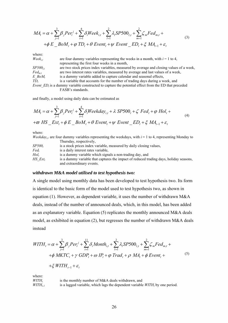
(3)

where: Weeki,t are four dummy variables representing the weeks in a month, with i = 1 to 4,

representing the first four weeks in a month, SP500l,t are two stock prices index variables, measured by average and closing values of a week, Fedm,t are two interest rates variables, measured by average and last values of a week, E_BoMt is a dummy variable added to capture calendar and seasonal effects, TDt is a variable that accounts for the number of trading days during a week, and Event_EDt is a dummy variable constructed to capture the potential effect from the ED that preceded

FASB’s standards. and finally, a model using daily data can be estimated as

3 4

,1 1

1

500

_ _ _

jt j t i i t t t

j i

t t t t t

MA Per Weekday SP Fed Hol

HS Ext E BoM Event Event ED MA

α β δ λ ζ ϕ

ϖ φ θ ψ ξ= =

−

+

+

= + + + + +

+ + + +

∑ ∑ε+

m t

+

(4)

where: Weekdayi,t are four dummy variables representing the weekdays, with i = 1 to 4, representing Monday to

Thursday, respectively, SP500t is a stock prices index variable, measured by daily closing values, Fedt is a daily interest rates variable, Holt is a dummy variable which signals a non-trading day, and HS_Extt is a dummy variable that captures the impact of reduced trading days, holiday seasons,

and extraordinary events. withdrawn M&A model utilised to test hypothesis two:

A single model using monthly data has been developed to test hypothesis two. Its form

is identical to the basic form of the model used to test hypothesis two, as shown in

equation (1). However, as dependent variable, it uses the number of withdrawn M&A

deals, instead of the number of announced deals, which, in this model, has been added

as an explanatory variable. Equation (5) replicates the monthly announced M&A deals

model, as exhibited in equation (2), but regresses the number of withdrawn M&A deals

instead

3 11 2 2

, ,,1 1 1 1

1

500jt j t i i t ml l t

j i l m

t t t t t t

tt

WITH Per Month SP Fed

MKTC GDP IP Trad MA Event

WITH

α β δ λ ζ

φ γ ω ϕ ρ φ

ξ ε

= = = =

−

= + + + + +

+ + + + + +

+ +

∑ ∑ ∑ ∑ (5)

where: WITHt is the monthly number of M&A deals withdrawn, and WITHt-1 is a lagged variable, which lags the dependent variable WITHt by one period.

26

5.5. Descriptive statistics for M&A activity

Table 2 shows descriptive statistics for unadjusted and non-dummy variables for the

whole period of study. Descriptive statistics for variables employed in the models using

monthly data are shown in Panel A. Apart interest rates variables, FED and FED Av, all

variables present low values of standard skewness and standard kurtosis. IP and GDP

have had a steady progress during the period of study, and therefore present the smallest

coefficients of variation, while FED variables exhibit the highest values. In terms of

dependent variables, WITH presents a higher coefficient variation than MA, situation

that can be regarded has natural, due to the reduced number of M&A cancellations, if

compared to the number of M&A announcements. The distribution shown by quartiles

also seem normal for all variables, although FED variables present lower and upper

quartiles very close to minimum and maximum values, respectively. A further analysis

of the histogram and the density trace for this variable revealed a double top, i.e., a high

concentration of observations around 2 % and 6 %, respectively.

[Please insert Table 2 about here]

The situation of the interest rates is a particular one, as the Federal Reserve, the central

bank of the U.S.A., commonly referred as “Fed”, was very active, in terms of monetary

policy, during 2001 and 2002. The US economy was in risk of recession and, in 2001,

the Fed started to cut aggressively the interest rates. If the average interest rates were

above 6 % in 2000, by the end of 2001 they were lower than 2 %. In 2002, the interest

rates would suffer further reductions, remaining at historically low levels.

Panel B exhibits descriptive statistics for variables employed in the model using weekly

data. The analysis is similar to the one made for Panel A. However, some descriptive

statistics deserve particular attention. Except for MA, the values of standard kurtosis are

outside the range of -2 to +2 for all variables. This range departure is also true for MA,

but only in terms of skewness. This situation suggests possible departures from

normality, since whenever kurtosis and skewness values are outside the range, there is a

greater possibility of invalidation of the statistical tests in respect of standard deviation.

On the other hand, this situation can be regarded as normal, since weekly data is

significantly more random than monthly data. Therefore, variables exhibiting signs of a

27

possible departure from normality, as a result, for example, of asymmetric distributions,

are expectable, since extreme observations became more evident in weekly data sets.

Finally, in terms of coefficients of variation, it has increased for MA, while FED

continued to exhibit the highest coefficient.

Descriptive statistics for variables employed in the model using daily data are presented

in Panel C. This panel is divided in sections (1) and (2). Section (1) presents descriptive

statistics for the whole period, while section (2) is centred on the analysis of the periods

that preceded and followed the effectiveness date of the new accounting rules.

In terms of descriptive statistics for the whole period, and comparing with the values of

the statistics previously examined, a further deterioration has been registered. The

coefficient of variation for MA has increased, and almost all values of kurtosis and

skewness are outside the range. An expected outcome, as if weekly data were more

random than monthly data, it would be for daily data to be on the extreme side of

randomness.

The observation of descriptive statistics for the period -391 to +391 days around 1 July

2001, shown in section (2), reveals better indicators for the period preceding the

effectiveness of the new accounting rules. In 2001, uncertainty ruled over U.S.A.

markets and economy, and turbulence increased with the September 11 terrorist attacks.

In addition to volatility, post event figures for M&A activity, stock prices indexes, and

interest rates, were significantly lower. Consequently, the coefficients of variation

increased for all variables, post eventum. This increase was particularly noteworthy for

interest rates, as result of the previously described Fed policy. A minimum and

maximum value of interest rates of 3.68 % and 7.03 % before 1 July 2001 compares

with rates in between 1.15 % and 3.89 % afterwards.

6. Results

6.1. Univariate analysis

Table 3 presents Pearson and Spearman correlation coefficients for several variables

taken from the long list. Correlation coefficients estimate the strength of the linear

28

relationship between the variables. The correlation coefficient ranges between -1 and

+1, representing -1 a perfect negative linear relationship, while, conversely, +1 indicates

perfect positive linear relationship. Coefficient values around zero value indicate

absence of linear relationship between variables. P-values, which test the statistical

significance of the estimated correlations, are exhibited in italic in Table 4. P-values

below 0.05 represent statistically significant non-zero correlations at the 95 %

confidence level. Unlike Pearson coefficients, Spearman correlation coefficients are

measured from ranks of data values rather than from data values themselves. As a result,

Pearson coefficients are more sensitive to outliers than Spearman coefficients.

[Please insert Table 3 about here]

A Pearson/Spearman correlation matrix of coefficient estimates for non-dummy

variables using monthly data is shown in Panel A. Apart coefficients for pairs of

variables involving TD, all correlations are significant at the 95 % confidence level.27

The only significant correlation for TD, at the 95 % level, is with MA, if measured by

Pearson correlations only. TD is also the variable with the lowest correlation

coefficients. This may be justified by the specific nature of this variable, which has the

characteristics of an adjustment variable, and consequently does not share the attributes

of the exogenous explanatory variables considered in the long list of variables.

Dependent variable MA presents higher correlation coefficients with explanatory

variables, than dependent variable WITH. Explanatory variables related to stock markets

indexes and capitalization, SP500, SP500 Av, and MKTC, are the ones who present the

highest correlations with the dependent variables, MA and WITH.

In terms of overall correlations between independent variables, the highest coefficient

values belong to variables that share similar features. It is the case of quasi-identical

pairs of variables, FED and FED Av, and SP500 and SP500 Av, which are measured by

final and average monthly values, and therefore share the same basis of construction. It

is also the case of stock markets variables, which include stock prices index variables,

SP500, and SP500 Av, and market capitalization variable, MKTC, because they share 27 More precisely, except for TD, all pairs present statistically significant non-zero correlations at the 99 % confidence level.

29

the same nature. Finally, time variables, Per, Per_2, and Per_3, are linearly related and

therefore present high mutual Pearson correlation coefficients. Spearman correlations

capture the linear dependence between variables in a different way. For the pairs of time

variables, Spearman correlation coefficients assume +1 value, indicating, as expected, a

perfect positive linear relationship between the variables.

A similar scenario is made visible in Panel B, where mutual correlations for non-

dummy variables to be tested in the model using weekly data are shown. All pairs of

variables present statistically significant non-zero correlations at the 99 % confidence

level, except for mutual correlations involving TD. The only significant correlation

involving TD is with MA, as it is also a non-zero correlation statistically significant at

the 99 % confidence level, if measured by Pearson correlations, and still significant, but

at the 95 % confidence level, if measured by Spearman correlations. Exogenous

explanatory variables, stock prices index and interest rates, continue to present high

correlation coefficients, as time variables as well. As in Panel A, in terms of overall

correlations, the highest coefficient values belong to subsets of variables that share the

same nature, have identical basis of construction, or are in linear dependence.

As Panel B, Panel C shows correlation coefficients for variables employed in models

developed to test hypothesis one, but using daily observations. Correlation coefficients

for dummy variables are also shown, except for weekday’s dummy variables.

Every pair of non-dummy variables presents statistically significant non-zero

correlations at the 99 % confidence level, while dummy variables only present

statistically significant correlations with dependent variable MA. The correlation

coefficients, which values have been reduced from monthly variables to weekly

variables, suffered a further reduction, as expected. Nevertheless, exogenous

explanatory variables and time variables continue to present significant correlation

coefficients, as dummy variables as well. The correlation of dummy variable E_BoM

and dependent variable MA constitutes a good example, as it presents a Pearson

correlation coefficient similar to the ones presented by pairs of MA and non-dummy

variables, namely, SP500, FED, and period.

30

The results obtained from univariate analysis corroborate, in general, the variables

predictions and the theory that has been discussed previously. GDP variable is the only

exception, as a positive correlation with MA would be expectable. However, GDP

variable is constructed using quarterly data, while MA is based on daily data.

Additionally, it has been referred that M&A activity is procyclical, as generally it leads

the business cycle (see e.g. Golbe & White, 1988; Nelson, 1959; Steiner, 1975; Weston

et al., 1990). Finally, the period subject to analysis is short. As a result from the

combination of these situations, a possible lag between M&A activity and GDP may

have passed unobserved, as the amount of elapsed time may have been insufficient to

capture the lag in a comprehensive way. The contradictory outcome that has been

discovered may be therefore justified by particular circumstantial conditions related to

business cycle and to M&A activity, which resulted in an occasional occurrence of

opposite trends, during a short period. It is feasible to admit this possibility, knowing

that M&A waves and business cycles lengths are often long, and that a lag of several

months may exist between these two different series. In resume, it may be simply the

case of a cutting point which captured the moment when only one of the variables

inverted the trend. In any case, an in depth examination of the reasons behind this

possible contradiction is not relevant for the present research. In addition, GDP variable

has not been selected by any model, following the backward elimination procedure that

has been applied to the long list of variables. Consequently, any risk of model

misspecification as a result of GDP inclusion is null.

6.2. Multivariate analysis

Table 4 presents the regression models outputs, and related conformity tests results as

well, for the models designed to test the research hypotheses. In Panels A, C, and D are

shown the outputs for equations (2), (3), and (4), respectively. All these models were

constructed with the purpose to test hypothesis one. Concurrently, Panel B exhibits the

output for equation (5), which has been conceived to test hypothesis two. Stepwise

regression, with backward elimination, has been employed in all models, resulting in

every variable left in the models to be significant at least at the 0.05 level.

[Please insert Table 4 about here]

31

models used to test hypothesis one:

As mentioned above, Panel A presents the results for the model constructed to test

hypothesis one, using monthly data. From the twenty-four variables initially considered,

only eight have been selected for the final model, as a consequence of the backward

elimination of sixteen variables. Fed and Per_3 variables are significant at the 0.05

level, while the remaining selected variables are also significant at the 0.01 level.

In terms of analysis of variance, F-ratio computed from ANOVA table is 68.49, with a

p-value less than 0.05, therefore indicating a statistically significant relationship

between the selected variables at the 95 % confidence level.

The R-Squared statistic is 0.9546, which indicates that the final model explains 95.4 %

of the variability in MA. Nevertheless, this statistic is not shown in Panel A, because the

adjusted R-squared statistic is more suitable for comparing models with different

numbers of independent variables. In this model, the R-squared adjusted for degrees of

freedom is 94.07 %. The standard error of the estimate presents a standard deviation of

the residuals of 28.05, while the mean absolute error (MAE), which measures the

average value of the residuals, is 19.33.

Regression with time series involves several issues that need to be addressed. For

example, it is necessary to examine a possible lack of independence in the residuals (see

e.g. Makridakis et al., 1998: 263). The Durbin-Watson (DW) is a classic statistical test,

used to detect the presence of autocorrelation in the residuals from a regression analysis.

The reference value for this statistic is two. In this case, DW statistic is 2.071, and the p-

value is 0.29, which is greater than 0.05. Therefore, there is no indication of serial

autocorrelation in the residuals at the 95 % confidence level.

Although not exhibited in Table 4, it is worthwhile to mention that estimated

autocorrelations and partial estimated autocorrelations, between values of residuals at

various lags, were also analysed. The examination of autocorrelations in residuals is

critical to check whether the time series may not well be completely random. In time

series, random numbers are often referred as noise. In estimated autocorrelations, the

lag k autocorrelation coefficient measures correlations between values of residuals at

32

time t and time t-k. For the model in analysis, the estimated autocorrelations coefficients

are contained within the 95 % probability limits for the twenty-four lags, meaning that

none of the autocorrelations coefficients is statistically significant at the 0.95 level. This

outcome indicates that the time series may well be completely random, being equivalent

to a white noise series.

Partial autocorrelations can be used to measure the degree of relationship between

lagged variables, Yt and Yt-k, when the effect of other time lags is removed, helping to

determine the order of autoregressive model needed to fit the data. It has been

previously mentioned that the long list of variables includes, for every model, a lagged

dependent variable, by one period. the lag k partial autocorrelation coefficient measures

correlations between values of residuals at time t and time t+k, having previously

accounted for the correlations at all lower lags. As in estimated autocorrelations, in this

model all partial autocorrelations are contained in the 95 % probability limits as well.

Therefore, the twenty-four partial autocorrelations coefficients are not statistically

significant at the 95.0% confidence level.

Concurrently, tests for randomness of residuals were also performed. This kind of tests

is used to examine whether residuals consist in a random sequence of numbers. Three

tests were run, although Table 4 exhibits the results for Box-Pierce test only: i) the first

test counts the number of times that the residuals sequence was above or below the

median. In this case, the number of runs was twenty, versus an expected number of

eighteen. The large sample test statistic Z is 0.5224; ii) the second test counts the

number of times the residuals sequence rises or fall. The number of runs up and down

was twenty-three, which matches with the expected number of runs up and down. Test

statistic Z value is 0.5224; and finally, iii) Box-Pierce test which is based on the sum of

squares of the first twenty-four autocorrelation coefficients.28 Every p-value for the

three tests performed is greater than 0.05, therefore the hypothesis that the series is

random at the 95 % or higher confidence level cannot be rejected.

Additional tests were also performed to examine the normality of residuals. These tests

are commonly used to find whether residuals can be adequately modelled by a normal

28 Tests descriptions made from Statgraphics’s tests reports and user’s guide (2006).

33

distribution. According to Statgraphics’s tests reports and user’s guide (2006): i) chi-

squared test divides the range of residuals into sixteen equally probable classes and

compares the number of observations in each class to the number expected based on the

fitted distribution; ii) Shapiro-Wilk W test is based upon comparing the quantiles of the

fitted normal distribution to the quantiles of the data; iii) standardized skewness test

examines for lack of symmetry in the data; and finally, iv) standardized kurtosis test

examines the distributional shape, which may be either flatter or more peaked than a

normal distribution. The p-values obtained for the tests are all greater than 0.05,

therefore the hypothesis that residuals comes from a normal distribution cannot be

rejected at the 95 % confidence level. Goodness-of-fit tests for residuals were also

performed: v) Kolmogorov-Smirnov (K-S) test computes the maximum distance

between the cumulative distribution of residuals and the cumulative distribution

function (CDF) of the fitted normal distribution. In this case, that maximum distance is

0.0816716; while vi) Kuiper V test compare the distribution function to the fitted CDF

in a different way. The p-values of K-S test, modified Kolmogorov-Smirnov D (K-S D)

test, Kuiper V test, and modified Kuiper V test, are also all greater than 0.05, which,

consequently, corroborates the previous indication of not rejecting the hypothesis that

residuals come from a normal distribution with 95% confidence.

In Panel C are shown the regression outputs for the model using weekly data. The

stepwise backward regression procedure resulted in the elimination of seven variables

from the initial sixteen. Nine variables have been therefore selected for the final model.

Every variable that was selected is significant at the 95 % confidence level, and only

FED and Week3 are not significant at the 99 % level as well. The construction of

ANOVA table provided a F-ratio value of 49.60, with a p-value inferior to 0.05, which

indicates the existence of a statistically significant relationship between the variables at

the 95 % confidence level.

The adjusted R-squared statistic indicates that the fitted model explains 73.95 % of the

variability in MA. The standard deviation of the residuals is 17.32, while the mean

absolute error of the residuals is 13.40. The comparison of these statistics with the ones

from the model using monthly data, allows one to observe a decrease on the predictive

power of the model, as adjusted R-squared value has decreased. On the other hand, a

34

reduction was recorded on the average value of the residuals and on the standard

deviation of the residuals.

Durbin-Watson statistic was used to test whether there is any significant correlation in

residuals. In this model, its value is 1.808. The p-value for DW statistic is 0.11729,

value greater than 0.05, which therefore indicates the inexistence of serial

autocorrelation in the residuals at the 95 % confidence level. In terms of estimated

autocorrelations for residuals, all twenty-four coefficients are contained in between the

95 % probability limits. Since the autocorrelations are not statistically significant at the

0.95 level, the time series are likely to be completely random.

As for the model using monthly data, three tests for randomness of residuals were

performed for the model using weekly data. Runs above and below median test has a

statistic Z value of 0.4042; runs up and down test has a statistic Z value of 1.2455; and

Box-Pierce test exhibits the value of 23.701. All the p-values for performed tests are

greater than 0.05. Consequently, the hypothesis that the series of residuals is random at

the 95 % confidence level cannot be rejected.

Except for Shapiro-Wilk W test, all tests performed to examine the normality of

residuals and the goodness-of-fit tests for residuals: chi-squared test, standardized

skewness, standardized kurtosis, Kolmogorov-Smirnov test, modified K-S D test,

Kuiper V test, and modified Kuiper V test, present p-values greater than 0.05. Since p-

value for Shapiro-Wilk W test is only greater than 0.01, the hypothesis that residuals

comes from a normal distribution can be rejected at the 95 % confidence level, but

cannot be rejected at the 99 % level. The lower p-value obtained for Shapiro-Wilk W

test can be regarded as normal. Whenever weekly or daily data is used, departures from

normality become a normal situation. For example, Marais (1984) found that weekly

residuals from CAR may deviate from normality with respect to skewness and kurtosis.

In fact, a few outliers can be enough to deviate a series from normality. It is important

to point out that the results presented at Table 4 include outliers, since its removal has

been made at the sensitivity analysis stage only.

Finally, Panel D exhibits the statistical outputs for the model using daily data. From the

initial fifteen variables, only four were removed: FED, Per_3, Event, and Event_ED.

35

All weekdays and remaining endogenous explanatory dummy variables were selected.

The lagged dependent variable, MA_lag, was also selected. Every variable that has been

selected is significant at the 95% and 99 % confidence level. The F-ratio from analysis

of variance is 95.34. Since its p-value is less than 0.05, there is a possible statistically

significant relationship between the variables at the 95 % confidence level.

The variability of MA is explained in 57.08 % by the final model. Alongside with the

decrease on the adjusted R-squared statistic, it has been also observed a further

reduction on the standard deviation of the residuals, from 17.32 to 6.69, and on the

MAE of the residuals, from 13.40 to 5.16.

The DW statistic assumes value 2.006, with a p-value of 0.46. Since the p-value is

greater than 0.05, there is no indication of a significant serial autocorrelation in the

residuals at the 95 % level. In terms of estimated autocorrelations for residuals, three of

the twenty-four autocorrelations coefficients are statistically significant at the 95 %

confidence level, suggesting that the time series may not be entirely random.

Nevertheless, when probability limits are eased to 99 %, none of the autocorrelations

coefficients are statistically significant, indicating, in opposition, that the time series

may well be completely random, but only at a lower confidence level.

As for statistical tests concerning the randomness of residuals, two of the performed

tests have a p-value greater than 0.05. It is the case of runs above and below median

test, and runs up and down test. However, Box-Pierce test presents a p-value which is

only greater than 0.01. Consequently, it can be rejected the hypothesis that the series is

random at the 95 % confidence level. Since the three tests are sensitive to different types

of departures from random behaviour, failure to pass any test suggests that the time

series may not be entirely random. Nevertheless, since the Box-Pierce test is still greater

than 0.01, the hypothesis that the series is random cannot be rejected at the 99 %

confidence level.

In terms of goodness-of-fit tests for residuals, which includes diverse tests, such as the

previously used Kuiper V and K-S tests, given that the smallest p-value amongst the

tests run is greater than 0.05, the hypothesis that residuals comes from a normal

distribution with 95 % confidence cannot be rejected. This conclusion is corroborated

36

by other tests for normality for residuals, such as chi-squared and Shapiro-Wilk tests,

which have a p-value higher than 0.05 as well. Nevertheless, skewness and kurtosis Z-

score’s exhibit very low p-values. Consequently, it can be rejected the idea that

residuals comes from a normal distribution with 95% confidence. As mentioned before,

the low p-values presented by standardized skewness and kurtosis match with the

situation portrayed by authors such as Marais (1984). It is important to recall that

departures from normality are common whenever weekly or daily data is used, and,

concurrently, outliers are likely to be kept in the models.

model used to test hypothesis two:

Panel B presents the estimation and tests results for equation (5). Since the model has

been developed in order to test hypothesis two, it uses WITH as dependent variable.

From the initial twenty-six monthly variables, eleven have been selected for the final

model, in detriment of other fifteen, which have been eliminated following the

backward elimination procedure. Oct and TD variables are significant at the 95 % level,

while the remaining variables are also significant at the 99 % level. The ANOVA F-

ratio is 20.80, and the p-value is less than 0.05, indicating a statistically significant

relationship between the variables at the 95 % confidence level.

The adjusted R-squared statistic indicates that the model as fitted explains 83.97 % of

the variability in the number of withdrawn M&A deals. In respect to residuals, the

standard deviation is 3.0221, and the MAE is 2.0852.

Durbin-Watson statistic is 2.28, with a p-value 0.51. Since DW p-value is greater than

0.05, there is no indication of the existence of serial autocorrelation in the residuals at

the 95 % confidence level. In terms of estimated autocorrelations for residuals, all

coefficients are contained in between the 95 % probability limits. Since the

autocorrelations are not statistically significant at the 0.95 level, the time series may

well be equivalent to white noise series.

In addition, the three tests for randomness of residuals which were performed in

previous models, present for this model p-values greater than 0.05. Therefore, it cannot

be rejected the hypothesis that the series of residuals is random at the 95 % confidence

level.

37

Finally, all tests performed for the normality and goodness-of-fit tests for residuals,

Kuiper V, K-S, K-S D, chi-squared, Shapiro-Wilk W, skewness and kurtosis Z-scores,

resulted in p-values greater than 0.05. Accordingly, the hypothesis that residuals comes

from a normal distribution cannot be rejected at the 95 % confidence level.

6.3. Sensitivity analysis

The analysis of statistical tests for all models did not raise relevant statistical issues,

concerning any possible models misspecification. During the early stage of models

development, weekends were removed from daily data series, to address the issue of

autocorrelation in the residuals. Observations from other non-trading days, resulting

from holidays and extraordinary events, were left in the models and treated with specific

dummy variables. The same treatment was given to reduced trading days.

The results obtained from ancillary regressions used to measure the effects of specific

extreme observations, alternative event windows, and alternative significance levels,

corroborate the main models outputs. They also corroborate the finding that the event

variables are insignificant at the 95% confidence level.

7. Conclusions

The findings show a significant positive relationship between M&A activity and stock

market prices, and also several significant associations between M&A and other

endogenous and exogenous explanatory variables, but no relationship between

accounting choice and M&A activity.

The intervention variables were not selected by any model constructed to test the

research hypothesis. Several sensitivity analyses, which included the examination of the

possible effects of extreme observations, non-trading days and reduced trading days;

and also assuming alternative event windows, and alternative significance levels, were

also carried out, with no implications on the main findings. The analysis of the impact

38

of possible outliers and influential points did not resulted in any chance on the research

findings as well.

Since the event variables were not able to reach even the 90% level of confidence

threshold, the research hypotheses cannot be rejected. Therefore, the findings indicate

that the effectiveness of the new accounting standards did not have any significant

impact on the M&A activity in the U.S.A., during the period subject to examination.

Financial markets conditions, time, and other M&A endogenous factors, proved more

influential than the changes in the accounting for business combinations in respect to

the pattern of M&A activity. This conclusion is consistent with the existing literature

which argues that the market is able to assess the underlying economics of the

transaction, regardless the accounting treatment (Davis, 1990; Hong et al., 1978;

Lindenberg & Ross, 1999; Vincent, 1997).

Finally, our findings prove that the compromise achieved between the FASB and the

different lobbies, particularly from IT and banking industries, did not harm the US

economy, since the M&A activity was not affected. Moreover, the present findings have

implications for several existing national sets of accounting standards which continue to

allow the use of pooling of interests method and the amortization of purchased

goodwill. This is the case in many countries in the Europe which have a dual accounting

system, based on the fourth and the seventh directives of the European Council, and on

the IASB standards that were recently endorsed by the EU. While IFRS 3 follows the

main guidelines of FASB standards, many of the existent national sets of GAAP in

Europe keep allowing pooling of interests and purchased goodwill amortization. We

therefore argue that national European standard setters should follow IASB GAAP to

enhance comparability among European companies involved in M&A deals.

39

References Aboody, D., R. Kasznik, & M. Williams. (2000). Purchase versus pooling in stock-for-

stock acquisitions: Why do firms care? Journal of Accounting & Economics,

29(3), 261-286.

Andrade, G., M. Mitchell, & E. Stafford. (2001). New Evidence and Perspectives on

Mergers. Journal of Economic Perspectives, 15(2), 103-120.

Andrade, G., & E. Stafford. (2004). Investigating the Economic Role of Mergers.

Journal of Corporate Finance, 10, 1-36.

Asquith, P. (1983). Merger Bids, Uncertainty, and Stockholder Returns. Journal of

Financial Economics, 11, 51-83.

Auster, E. R., & M. L. Sirower. (2002). The Dynamics of Merger and Acquisition

Waves: A Three-Stage Conceptual Framework with Implications for Practice.

Journal of Applied Behavioral Science, 38(2), 216-244.

Ayers, B., C. Lefanowicz, & J. Robinson. (2002). Do firms purchase the pooling

method? Review of Accounting Studies, 7, 5-32.

Barkoulas, J. T., C. F. Baum, & A. Chakraborty. (2001). Waves and persistence in

merger and acquisition activity. Economics Letters, 70(2), 237–243.

Beckenstein, A. R. (1979). Merger activity and merger theories: An empirical

investigation. Antitrust Bulletin, 24, 105-128.

Becketti, S. (1986). Corporate mergers and the business cycle. Economic Review, 71,

13-26.

Brealey, R., & S. Myers. (1984). Principles of Corporate Finance. New York:

McGraw-Hill, Inc.

Brealey, R., & S. Myers. (1996). Principles of Corporate Finance. New York:

McGraw-Hill, Inc.

Brealey, R., S. Myers, & F. Allen. (2006). Principles of Corporate Finance. New York:

McGraw-Hill, Inc.

Brockwell, P. J., & R. A. Davis. (1996). An Introduction to Time Series and

Forecasting. New York, NY: Springer-Verlag.

Chowdhury, A. R. (1993). Univariate time-series behaviour of merger activity and its

various components in the United States. Applied Financial Economics, 3(1),

61–66.

40

Davidson III, W. N., S. Rosenstein, & S. Sundaram. (2002). An Empirical analysis of

cancelled mergers, board composition and ownership structure. Applied

Financial Economics, 12, 485-491.

Davis, M. L. (1990). Differential market reaction to pooling and purchase methods. The

Accounting Review, 65, 696-709.

Dodd, P. (1980). Merger proposals, management discretion, and stockholder wealth.

Journal of Financial Economics, 8(June), 105-137.

Dong, M., D. Hirshleifer, S. Richardson, & S. H. Teoh. (2006). Does investor

misvaluation drive the takeover market? Journal of Finance, 61, 725-762.

Draper, N. R., & H. Smith. (1981). Applied Regression Analysis (2nd ed.). New York,

NY: John Wiley & Sons, Inc.

Dunne, K. M. (1990). An empirical analysis of managements choice of accounting

treatment for business combinations. Journal of Accounting & Economics, 9(2),

111-133.

Eis, C. (1969). The 1919-1930 merger movement in American industry. The Journal of

Law and Economics, 12(2), 267-296.

FASB. (2001). FASB Completes Business Combinations Project. Financial Accounting

Standards Board at www.fasb.org (July, 5).

Fields, T. D., T. Z. Lys, & L. Vincent. (2001). Empirical research on accounting choice.

Journal of Accounting & Economics, 31(1-3), 255-307.

Franks, J. R., & C. Mayer. (1996). Hostile takeovers and the correction of managerial

failure. Journal of Financial Economics, 40, 163-181.

Gagnon, J. (1967). Purchase versus pooling of interests: The search for a predictor.

Journal of Accounting Research, Empirical Research in Accounting: Selected

Studies, Supplement to Vol. 5, 187-204.

Golbe, D. L., & L. J. White. (1988). A Time-Series Analysis of Mergers and

Acquisitions in the U.S. Economy. In A. J. Auerbach (Ed.), Corporate

Takeovers: Causes and Consequences (pp. 265-302). Chicago, IL: University of

Chicago Press / NBER.

Golbe, D. L., & L. J. White. (1993). Catch a Wave: The Time Series Behavior of

Mergers. The Review of Economics and Statistics, 75(3), 493-499.

Gort, M. (1969). An economic disturbance theory of mergers. Quarterly Journal of

Economics, 83(4), 624-642.

41

Guerard, J. B. J. (1985). Mergers, Stock Prices, and Industrial Production: An Empirical

Test of the Nelson Hypothesis In O. D. Anderson (Ed.), Time Series Analysis:

Theory and Practice (Vol. 7). Amsterdam: Elsevier.

Halpern, P. J. (1973). Empirical Estimates of the Amount and Distribution of Gains to

Companies in Mergers. Journal of Business, 46, 554-575.

Harford, J. (2005). What drives merger waves? Journal of Financial Economics, 77(3),

529-560.

Hirsch, J. A. (2004). Stock Trader's Almanac 2005 (38th ed.). Hoboken, NJ: John Wiley

& Sons, Inc.

Hocking, R. R. (1976). The analysis and selection of variables in linear regression.

Biometrics, 32, 1-50.

Holl, P., & D. Kyriazis. (1996). The Determinants of Outcome in UK Takeover Bids.

International Journal of the Economics of Business, 3, 165-184.

Holmstrom, B., & S. N. Kaplan. (2001). Corporate governance and merger activity in

the United States: Making sense of the 1980s and 1990s. Journal of Economic

Perspectives, 15(2), 121-144.

Hong, H., R. S. Kaplan, & G. Mandelker. (1978). Pooling vs. Purchase: The Effects of

Accounting for Mergers on Stock Prices. The Accounting Review, 53(1), 31-47.

Hopkins, P. E., R. W. Houston, & M. F. Peters. (2000). Purchase, Pooling, and Equity

Analysts' Valuation Judgments. The Accounting Review, 75(3), 257-281.

Jennings, R., J. Robinson, R. Thompson, & L. Duvall. (1996). The relation between

accounting goodwill numbers and equity values. Journal of Business Finance

and Accounting, 23, 513-533.

Judge, G. G., R. C. Hill, W. E. Griffiths, H. Lütkepohl, & T.-C. Lee. (1988).

Introduction to the Theory and Practice of Econometrics (2nd ed.). New York:

John Wiley & Sons, Inc.

Karpoff, J. M., P. H. Malatesta, & R. A. Walkling. (1996). Corporate governance and

shareholder initiatives: empirical evidence. Journal of Financial Economics, 42,

365-395.

Lindenberg, E., & M. P. Ross. (1999). To purchase or to pool? Does it matter? Journal

of Applied Corporate Finance, 12(2), 32-47.

Linsmeier, T. J., J. R. Boatsman, R. H. Herz, R. G. Jennings, G. J. Jonas, M. H. Lang, et

al. (1998). Response to FASB Special Report, “Issues Associated with the

FASB Project on Business Combinations". Accounting Horizons, 12, 87-89.

42

Lys, T., & L. Vincent. (1995). An Analysis of Value Destruction in AT&T’s

Acquisition of NCR. Journal of Financial Economics, 39, 353-378.

Makridakis, S., S. C. Wheelwright, & R. J. Hyndman. (1998). Forecasting: Methods

and Applications (3th ed.). NY: John Wiley & Sons, Inc.

Mandelker, G. (1974). Risk and return: the case of merging firms. Journal of Financial

Economics, 1, 303-335.

Marais, M. L. (1984). An application of the bootstrap method to the analysis of squared,

standardized market model prediction errors. Journal of Accounting Research,

22(Supplement), 34-54.

Markham, J. W. (1955). Survey of the evidence and findings on mergers. In Business

concentration and price policy (pp. 141-212). Princeton, NJ: Princeton

University Press.

Martinez-Jerez, F. (2001). Capital markets assessment of accounting for business

combinations. Harvard University Working paper.

Melicher, R. W., J. Ledolter, & L. J. D'Antonio. (1983). A Time Series Analysis of

Aggregate Merger Activity. The Review of Economic Statistics, 65(3), 423-430.

Mergerstat. (2003). Mergerstat Review 2003. Los Angeles, California: FactSet

Mergerstat, LLC.

Mitchell, M. L., & J. H. Mulherin. (1996). The impact of industry shocks on takeover

and restructuring activity. Journal of Financial Economics, 41(2), 193-229.

Muehlfeld, K., P. R. Sahib, & A. van Witteloostuijn. (2006). Completion or

abandonment of mergers and acquisitions. Working Paper.

Mueller, D. C. (Ed.). (1980). The Determinants and Effects of Mergers. Cambridge,

MA: Oelgeschlager, Gunn & Hain Publishers, Inc.

Nelson, R. L. (1959). Merger Movements in American Industry: 1895-1956. Princeton,

NJ: Princeton University Press.

Pickering, J. F. (1978). The Abandonment of Major Mergers in the U.K. 1965-1975.

Journal of Industrial Economics, 27, 123-131.

Prepared Testimony of Mr. Dennis Powell Vice President and Corporate Controller

Cisco Systems, Senate Banking Committee, Hearing on Pooling Accounting

Sess. (2000).

Prepared Testimony of Mr. James Barksdale Partner The Barksdale Group, Senate

Banking Committee, Hearing on Pooling Accounting Sess. (2000).

43

Rhodes-Kropf, M., D. T. Robinson, & S. Viswanathan. (2005). Valuation waves and

merger activity: The empirical evidence. Journal of Financial Economics, 77,

561-603.

Rhodes-Kropf, M., & S. Viswanathan. (2004). Market valuation and merger waves.

Journal of Finance, 59(6), 2685-2718.

Robinson, J. R., & P. B. Shane. (1990). Acquisition accounting method and bid

premium for target firms. The Accounting Review, 65(1), 25-48.

Shleifer, A., & R. W. Vishny. (2003). Stock market driven acquisitions. Journal of

Financial Economics, 70, 295-311.

Shughart II, W. F., & R. D. Tollison. (1984). The Random Character of Merger

Activity. The Rand Journal of Economics, 15(4), 500-509.

Steiner, P. O. (1975). Mergers: motives, effects, policies. Ann Arbor, MI: University of

Michigan Press.

Stigler, G. J. (1950). Monopoly and oligopoly by merger. The American Economic

Review, 40(2), 23-34.

Sudarsanam, P. S. (2003). Creating Value from Mergers and Acquisitions. Harlow,

Essex: Pearson Education.

Thomson Financial. (2006). SDC Platinum database: Thomson Financial.

Town, R. J. (1992). Merger Waves and the Structure of Merger and Acquisition Time-

Series. Journal of Applied Econometrics, 7(Supplement: Special Issue on

Nonlinear Dynamics and Econometrics), S83-S100.

Vincent, L. (1997). Equity valuation implications of purchase versus pooling

accounting. Journal of Financial Statement Analysis, 2, 5-19.

Walter, J. R. (1999). Pooling or Purchase: a Merger Mystery. Federal Reserve Bank of

Richmond Economic Quarterly, 85, 27-46.

Watts, R. L., & J. L. Zimmerman. (1990). Positive accounting theory: a ten year

perspective. The Accounting Review, 65(1), 131-156.

Weber, J. P. (2004). Shareholder wealth effects of pooling-of-interests accounting:

evidence from the SEC's restriction on share repurchases following pooling

transactions. Journal of Accounting & Economics, 37(1), 39-57.

Weston, J. F. (1953). The Role of Mergers in the Growth of Large Firms. Berkeley and

Los Angeles: University of California Press.

Weston, J. F., K. S. Chung, & S. E. Hoag. (1990). Takeovers, Restructuring and

Corporate Governance (1st ed.). Englewood Cliffs: Prentice Hall.

44

Weston, J. F., M. L. Mitchell, & J. H. Mulherin. (2004). Takeovers, Restructuring and

Corporate Governance (4th ed.). Upper Saddle River, NJ: Pearson Education.

Wong, P., & N. O’Sullivan. (2001). The Determinants and Consequences of Abandoned

Takeovers. Journal of Economic Surveys, 15, 145-186.

45

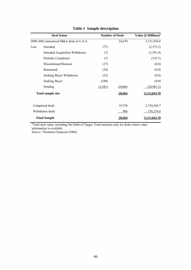
46

Table 1 Sample description

Deal Status Number of Deals Value ($ Millions)a

2000-2002 announced M&A deals in U.S.A 24,670 3,151,924.6

Less Intended (77) (2,573.2)

Intended Acquisition Withdrawn (7) (1,391.0)

Partially Completed (7) (335.5)

Discontinued Rumour (17) (0.0)

Rumoured (54) (0.0)

Seeking Buyer Withdrawn (23) (0.0)

Seeking Buyer (240) (0.0)

Pending (3,581) (4,006) (34,981.2)

Total sample size 20,664 3,112,643.70

Completed deals 19,758 2,734,269.7

Withdrawn deals 906 378,374.0

Final Sample 20,664 3,112,643.70

aTotal deal value, including Net Debt of Target. Total amounts only for deals where value information is available. Source: Thomson Financial (2006).

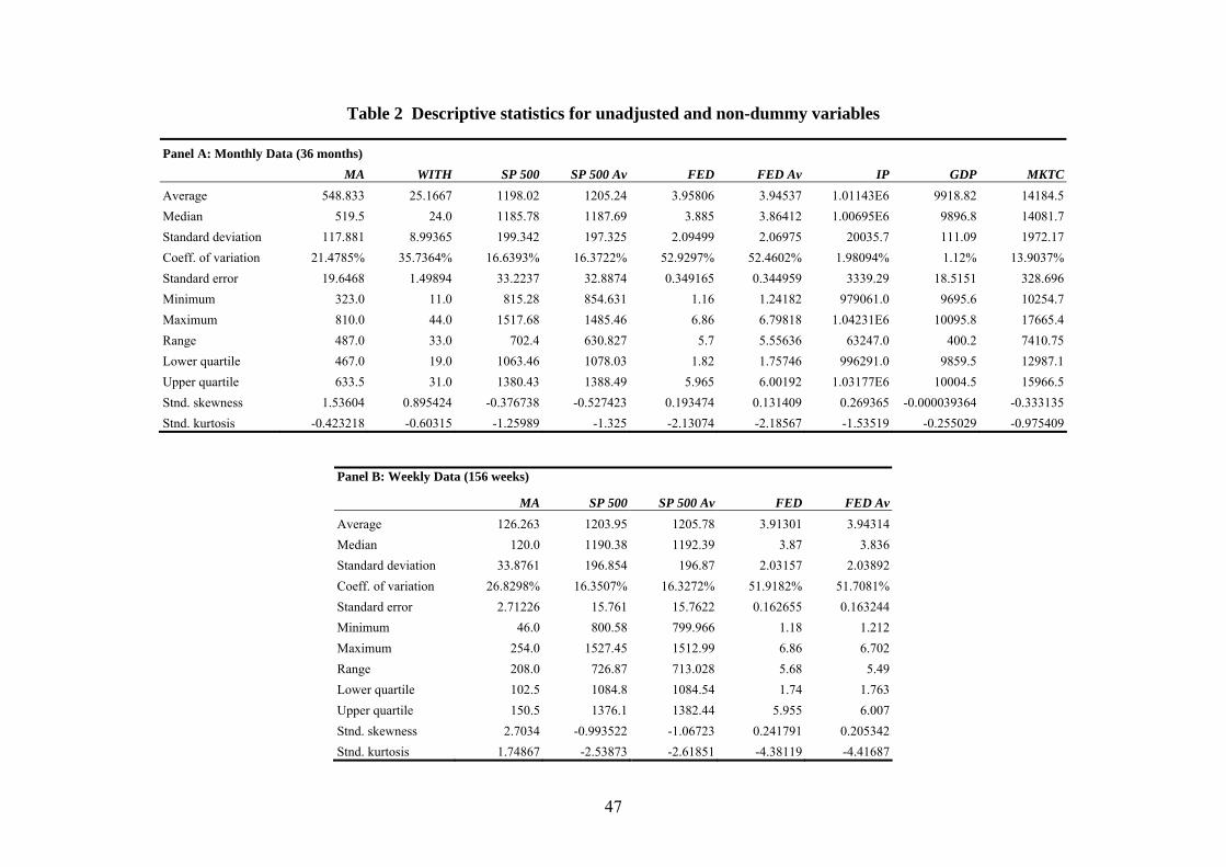
Table 2 Descriptive statistics for unadjusted and non-dummy variables

Panel A: Monthly Data (36 months) MA WITH SP 500 SP 500 Av FED FED Av IP GDP MKTC

Average 548.833 25.1667 1198.02 1205.24 3.95806 3.94537 1.01143E6 9918.82 14184.5Median 519.5 24.0 1185.78 1187.69 3.885 3.86412 1.00695E6 9896.8 14081.7Standard deviation 117.881 8.99365 199.342 197.325 2.09499 2.06975 20035.7 111.09 1972.17Coeff. of variation 21.4785% 35.7364% 16.6393% 16.3722% 52.9297% 52.4602% 1.98094% 1.12% 13.9037%Standard error 19.6468 1.49894 33.2237 32.8874 0.349165 0.344959 3339.29 18.5151 328.696Minimum 323.0 11.0 815.28 854.631 1.16 1.24182 979061.0 9695.6 10254.7Maximum 810.0 44.0 1517.68 1485.46 6.86 6.79818 1.04231E6 10095.8 17665.4Range 487.0 33.0 702.4 630.827 5.7 5.55636 63247.0 400.2 7410.75Lower quartile 467.0 19.0 1063.46 1078.03 1.82 1.75746 996291.0 9859.5 12987.1Upper quartile 633.5 31.0 1380.43 1388.49 5.965 6.00192 1.03177E6 10004.5 15966.5Stnd. skewness 1.53604 0.895424 -0.376738 -0.527423 0.193474 0.131409 0.269365 -0.000039364 -0.333135Stnd. kurtosis -0.423218 -0.60315 -1.25989 -1.325 -2.13074 -2.18567 -1.53519 -0.255029 -0.975409

Panel B: Weekly Data (156 weeks)

MA SP 500 SP 500 Av FED FED AvAverage 126.263 1203.95 1205.78 3.91301 3.94314Median 120.0 1190.38 1192.39 3.87 3.836Standard deviation 33.8761 196.854 196.87 2.03157 2.03892Coeff. of variation 26.8298% 16.3507% 16.3272% 51.9182% 51.7081%Standard error 2.71226 15.761 15.7622 0.162655 0.163244Minimum 46.0 800.58 799.966 1.18 1.212Maximum 254.0 1527.45 1512.99 6.86 6.702Range 208.0 726.87 713.028 5.68 5.49Lower quartile 102.5 1084.8 1084.54 1.74 1.763Upper quartile 150.5 1376.1 1382.44 5.955 6.007Stnd. skewness 2.7034 -0.993522 -1.06723 0.241791 0.205342Stnd. kurtosis 1.74867 -2.53873 -2.61851 -4.38119 -4.41687

47

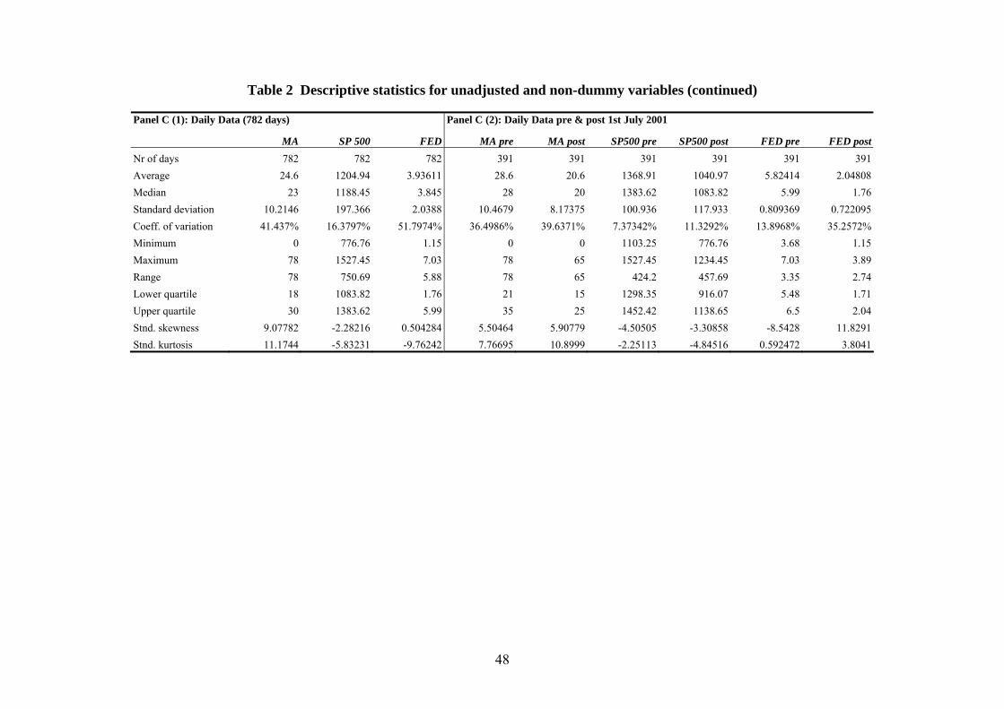
Table 2 Descriptive statistics for unadjusted and non-dummy variables (continued)

Panel C (1): Daily Data (782 days) Panel C (2): Daily Data pre & post 1st July 2001

MA SP 500 FED MA pre MA post SP500 pre SP500 post FED pre FED postNr of days 782 782 782 391 391 391 391 391 391Average 24.6 1204.94 3.93611 28.6 20.6 1368.91 1040.97 5.82414 2.04808Median 23 1188.45 3.845 28 20 1383.62 1083.82 5.99 1.76Standard deviation 10.2146 197.366 2.0388 10.4679 8.17375 100.936 117.933 0.809369 0.722095Coeff. of variation 41.437% 16.3797% 51.7974% 36.4986% 39.6371% 7.37342% 11.3292% 13.8968% 35.2572%Minimum 0 776.76 1.15 0 0 1103.25 776.76 3.68 1.15Maximum 78 1527.45 7.03 78 65 1527.45 1234.45 7.03 3.89Range 78 750.69 5.88 78 65 424.2 457.69 3.35 2.74Lower quartile 18 1083.82 1.76 21 15 1298.35 916.07 5.48 1.71Upper quartile 30 1383.62 5.99 35 25 1452.42 1138.65 6.5 2.04Stnd. skewness 9.07782 -2.28216 0.504284 5.50464 5.90779 -4.50505 -3.30858 -8.5428 11.8291Stnd. kurtosis 11.1744 -5.83231 -9.76242 7.76695 10.8999 -2.25113 -4.84516 0.592472 3.8041

48

Table 3 Pearson/Spearman correlation matrixes for coefficient estimates

Panel A: Monthly observations

MA WITH SP500 SP500 Av FED FED Av IP GDP MKTC Per Per_2 Per_3 TD

MA 0.7390 0.8194 0.8021 0.8004 0.7671 0.7968 -0.6926 0.8227 -0.8216 -0.7114 -0.6185 0.3454 0.0000 0.0000 0.0000 0.0000 0.0000 0.0000 0.0000 0.0000 0.0000 0.0000 0.0001 0.0391WITH 0.7098 0.7521 0.7659 0.7075 0.6765 0.6920 -0.6163 0.7489 -0.7363 -0.6766 -0.6213 0.1513 0.0000 0.0000 0.0000 0.0000 0.0000 0.0000 0.0001 0.0000 0.0000 0.0000 0.0001 0.3783SP500 0.8384 0.7501 0.9885 0.9065 0.9024 0.7115 -0.8552 0.9894 -0.9464 -0.9379 -0.8978 0.0971 0.0000 0.0000 0.0000 0.0000 0.0000 0.0000 0.0000 0.0000 0.0000 0.0000 0.0000 0.5731SP500 Av 0.8311 0.7582 0.9876 0.9163 0.9104 0.7150 -0.8634 0.9721 -0.9543 -0.9487 -0.9105 0.0576 0.0000 0.0000 0.0000 0.0000 0.0000 0.0000 0.0000 0.0000 0.0000 0.0000 0.0000 0.7384FED 0.8000 0.6944 0.8879 0.9019 0.9933 0.8562 -0.7906 0.8565 -0.9396 -0.9139 -0.8492 0.1069 0.0000 0.0000 0.0000 0.0000 0.0000 0.0000 0.0000 0.0000 0.0000 0.0000 0.0000 0.5350FED Av 0.7995 0.6550 0.8947 0.9017 0.9539 0.8496 -0.7816 0.8509 -0.9292 -0.9133 -0.8526 0.0744 0.0000 0.0001 0.0000 0.0000 0.0000 0.0000 0.0000 0.0000 0.0000 0.0000 0.0000 0.6665IP 0.7727 0.6702 0.6963 0.7066 0.7681 0.7596 -0.4755 0.6615 -0.7264 -0.6184 -0.5040 0.1189 0.0000 0.0001 0.0000 0.0000 0.0000 0.0000 0.0034 0.0000 0.0000 0.0001 0.0017 0.4899GDP -0.7049 -0.6276 -0.8645 -0.8846 -0.8568 -0.8311 -0.5600 -0.8455 0.9303 0.9207 0.8968 0.0401 0.0000 0.0002 0.0000 0.0000 0.0000 0.0000 0.0009 0.0000 0.0000 0.0000 0.0000 0.8162MKTC 0.8301 0.7342 0.9848 0.9735 0.8503 0.8541 0.6438 -0.8373 -0.9146 -0.9062 -0.8705 0.1315 0.0000 0.0000 0.0000 0.0000 0.0000 0.0000 0.0001 0.0000 0.0000 0.0000 0.0000 0.4447Per -0.8273 -0.7209 -0.9403 -0.9418 -0.9229 -0.9009 -0.6862 0.9411 -0.9094 0.9700 0.9195 -0.0256 0.0000 0.0000 0.0000 0.0000 0.0000 0.0000 0.0000 0.0000 0.0000 0.0000 0.0000 0.8821Per_2 -0.8273 -0.7209 -0.9403 -0.9418 -0.9229 -0.9009 -0.6862 0.9411 -0.9094 1.0000 0.9862 -0.0107 0.0000 0.0000 0.0000 0.0000 0.0000 0.0000 0.0000 0.0000 0.0000 0.0000 0.0000 0.9508Per_3 -0.8273 -0.7209 -0.9403 -0.9418 -0.9229 -0.9009 -0.6862 0.9411 -0.9094 1.0000 1.0000 0.0035 0.0000 0.0000 0.0000 0.0000 0.0000 0.0000 0.0000 0.0000 0.0000 0.0000 0.0000 0.9837TD 0.2666 0.0840 0.0535 0.0306 0.1244 0.1137 0.0216 0.0173 0.0513 -0.0133 -0.0133 -0.0133 0.1148 0.6192 0.7514 0.8563 0.4616 0.5010 0.8982 0.9187 0.7614 0.9373 0.9373 0.9373

Upper-right cells and lower-left cells diagonal represent Pearson and Spearman correlation coefficients, respectively. P-Values in italic. Only non-dummy variables are exhibited. 36 monthly observations.

49

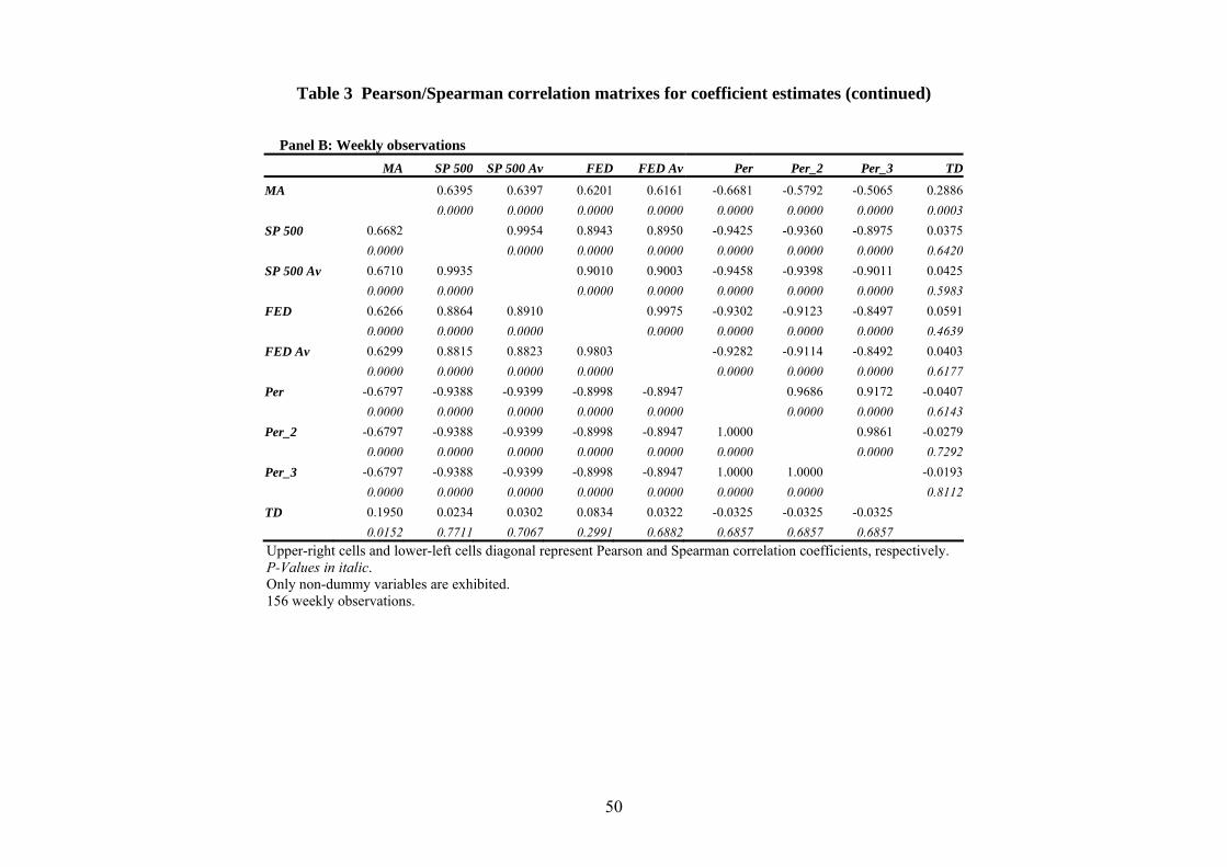
Table 3 Pearson/Spearman correlation matrixes for coefficient estimates (continued)

Panel B: Weekly observations MA SP 500 SP 500 Av FED FED Av Per Per_2 Per_3 TD

MA 0.6395 0.6397 0.6201 0.6161 -0.6681 -0.5792 -0.5065 0.2886 0.0000 0.0000 0.0000 0.0000 0.0000 0.0000 0.0000 0.0003SP 500 0.6682 0.9954 0.8943 0.8950 -0.9425 -0.9360 -0.8975 0.0375 0.0000 0.0000 0.0000 0.0000 0.0000 0.0000 0.0000 0.6420SP 500 Av 0.6710 0.9935 0.9010 0.9003 -0.9458 -0.9398 -0.9011 0.0425 0.0000 0.0000 0.0000 0.0000 0.0000 0.0000 0.0000 0.5983FED 0.6266 0.8864 0.8910 0.9975 -0.9302 -0.9123 -0.8497 0.0591 0.0000 0.0000 0.0000 0.0000 0.0000 0.0000 0.0000 0.4639FED Av 0.6299 0.8815 0.8823 0.9803 -0.9282 -0.9114 -0.8492 0.0403 0.0000 0.0000 0.0000 0.0000 0.0000 0.0000 0.0000 0.6177Per -0.6797 -0.9388 -0.9399 -0.8998 -0.8947 0.9686 0.9172 -0.0407 0.0000 0.0000 0.0000 0.0000 0.0000 0.0000 0.0000 0.6143Per_2 -0.6797 -0.9388 -0.9399 -0.8998 -0.8947 1.0000 0.9861 -0.0279 0.0000 0.0000 0.0000 0.0000 0.0000 0.0000 0.0000 0.7292Per_3 -0.6797 -0.9388 -0.9399 -0.8998 -0.8947 1.0000 1.0000 -0.0193 0.0000 0.0000 0.0000 0.0000 0.0000 0.0000 0.0000 0.8112TD 0.1950 0.0234 0.0302 0.0834 0.0322 -0.0325 -0.0325 -0.0325 0.0152 0.7711 0.7067 0.2991 0.6882 0.6857 0.6857 0.6857 Upper-right cells and lower-left cells diagonal represent Pearson and Spearman correlation coefficients, respectively. P-Values in italic. Only non-dummy variables are exhibited. 156 weekly observations.

50

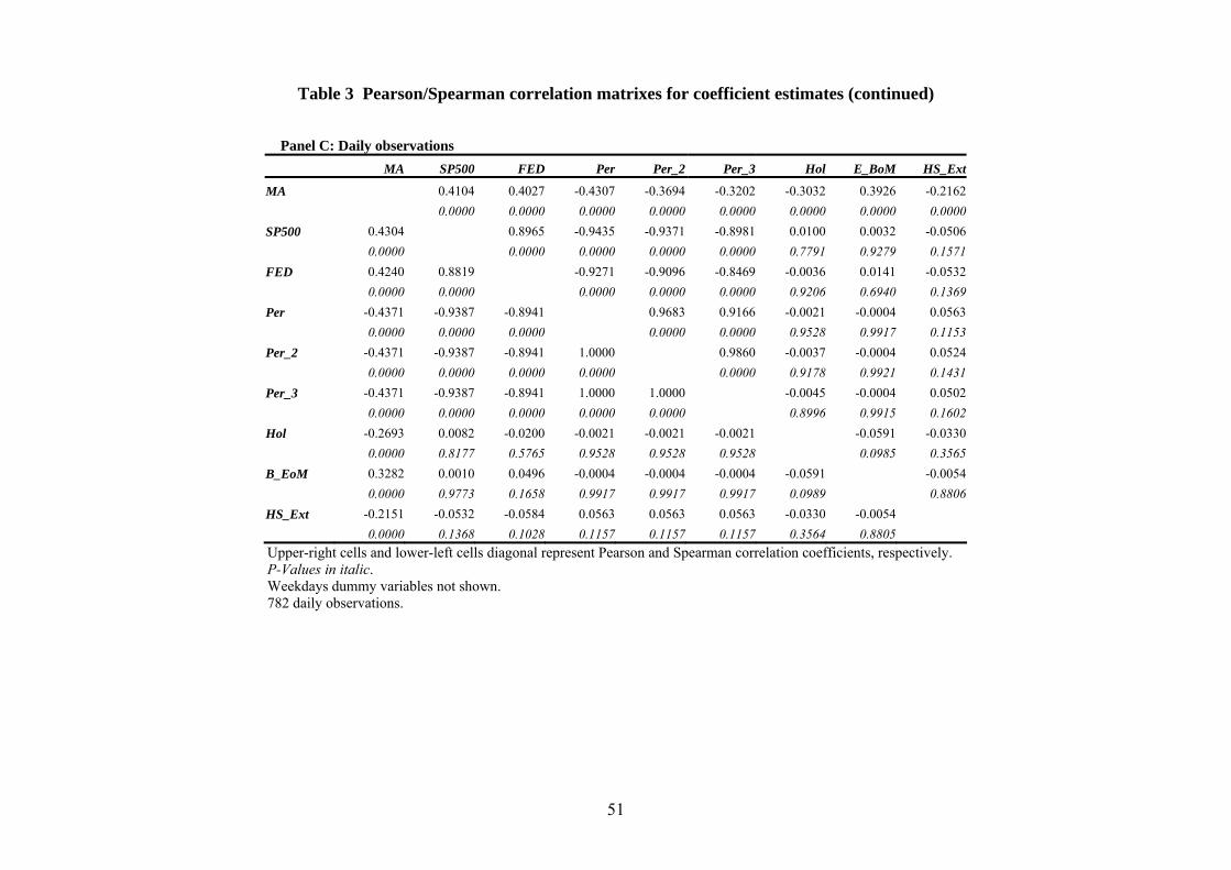
51

Table 3 Pearson/Spearman correlation matrixes for coefficient estimates (continued)

Panel C: Daily observations MA SP500 FED Per Per_2 Per_3 Hol E_BoM HS_Ext

MA 0.4104 0.4027 -0.4307 -0.3694 -0.3202 -0.3032 0.3926 -0.2162 0.0000 0.0000 0.0000 0.0000 0.0000 0.0000 0.0000 0.0000SP500 0.4304 0.8965 -0.9435 -0.9371 -0.8981 0.0100 0.0032 -0.0506 0.0000 0.0000 0.0000 0.0000 0.0000 0.7791 0.9279 0.1571FED 0.4240 0.8819 -0.9271 -0.9096 -0.8469 -0.0036 0.0141 -0.0532 0.0000 0.0000 0.0000 0.0000 0.0000 0.9206 0.6940 0.1369Per -0.4371 -0.9387 -0.8941 0.9683 0.9166 -0.0021 -0.0004 0.0563 0.0000 0.0000 0.0000 0.0000 0.0000 0.9528 0.9917 0.1153Per_2 -0.4371 -0.9387 -0.8941 1.0000 0.9860 -0.0037 -0.0004 0.0524 0.0000 0.0000 0.0000 0.0000 0.0000 0.9178 0.9921 0.1431Per_3 -0.4371 -0.9387 -0.8941 1.0000 1.0000 -0.0045 -0.0004 0.0502 0.0000 0.0000 0.0000 0.0000 0.0000 0.8996 0.9915 0.1602Hol -0.2693 0.0082 -0.0200 -0.0021 -0.0021 -0.0021 -0.0591 -0.0330 0.0000 0.8177 0.5765 0.9528 0.9528 0.9528 0.0985 0.3565B_EoM 0.3282 0.0010 0.0496 -0.0004 -0.0004 -0.0004 -0.0591 -0.0054 0.0000 0.9773 0.1658 0.9917 0.9917 0.9917 0.0989 0.8806HS_Ext -0.2151 -0.0532 -0.0584 0.0563 0.0563 0.0563 -0.0330 -0.0054 0.0000 0.1368 0.1028 0.1157 0.1157 0.1157 0.3564 0.8805 Upper-right cells and lower-left cells diagonal represent Pearson and Spearman correlation coefficients, respectively. P-Values in italic. Weekdays dummy variables not shown. 782 daily observations.

Table 4 Regression models outputs and tests results

3 11 2 2

, , ,1 1 1 1

1

500jt j t i i t l l t m m t

j i l m

t t t t t t

tMA Per Month SP Fed IP

MKTC GDP TD Event MA

α β δ λ ζ ω

φ γ ϕ θ ξ ε= = = =

−

= + + + + + +

+ + + + + +

∑ ∑ ∑ ∑ (2)

Backward elimination regression, with all variables left in the model significant at the 0.05 level:

Panel A: Estimation and tests results for model using M&A monthly data T Standard Parameter Estimate P-Value Statistic Error

Intercept -245.992 0.1057 -1.67637 146.741 Per -38.3226 0.0001 -4.68077 8.18724 Per_2 2.05267 0.0047 3.08964 0.664373 Per_3 -0.02809 0.0242 -2.3933 0.011735 Aug -58.0454 0.0039 -3.16688 18.3289 Nov -52.9105 0.0060 -2.99344 17.6755 SP500 0.35015 0.0003 4.23733 0.082635 Fed 32.7201 0.0297 2.30109 14.2194 TD 18.6442 0.0000 5.36609 3.47444

ANOVA F value 68.49 0.0000 R-squared 95.4696% R2 Adjusted for d. f. 94.0756% N used (read) 35 (36) Durbin-Watson D 2.07124 0.2912 Chi-Squared (13 d. f.) 4.77137 0.979887 Shapiro-Wilk W 0.955366 0.212621 Skewness Z-score 1.37276 0.169827 Kurtosis Z-score 1.10334 0.269877 Kolmogorov-Smirnov 0.0816716 0.973699 Modified K-S D 0.494093 ≥ 0.10* Cramer-Von Mises W2 0.048242 0.525551* Watson U2 0.0384931 0.645844* Anderson-Darling A2 0.386077 0.372269* Kuiper V 0.152129 ≥ 0.10* Box-Pierce Test 8.90604 0.630565

* P-Value has been compared to tables of critical values specially constructed for fitting the selected distribution. Except for the Chi-Squared Test, other P-values are based on general tables.

52

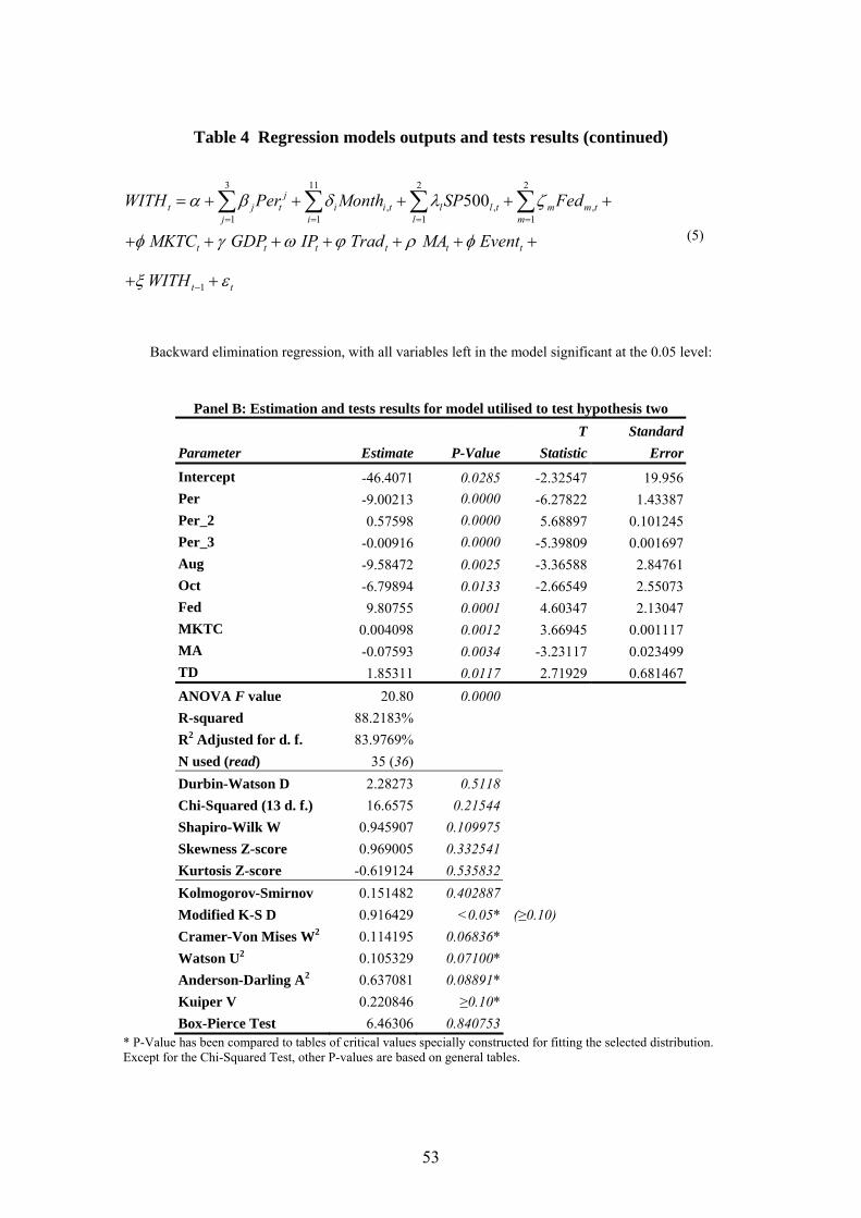
Table 4 Regression models outputs and tests results (continued)

3 11 2 2

, ,1 1 1 1

1

500jt j t i i t l l t m

j i l m

t t t t t t

t t

WITH Per Month SP Fed

MKTC GDP IP Trad MA Event

WITH

α β δ λ ζ

φ γ ω ϕ ρ φ

ξ ε

= = = =

−

= + + + + +

+ + + + + + +

+ +

∑ ∑ ∑ ∑ ,m t

(5)

Backward elimination regression, with all variables left in the model significant at the 0.05 level:

Panel B: Estimation and tests results for model utilised to test hypothesis two T Standard Parameter Estimate P-Value Statistic Error

Intercept -46.4071 0.0285 -2.32547 19.956 Per -9.00213 0.0000 -6.27822 1.43387 Per_2 0.57598 0.0000 5.68897 0.101245 Per_3 -0.00916 0.0000 -5.39809 0.001697 Aug -9.58472 0.0025 -3.36588 2.84761 Oct -6.79894 0.0133 -2.66549 2.55073 Fed 9.80755 0.0001 4.60347 2.13047 MKTC 0.004098 0.0012 3.66945 0.001117 MA -0.07593 0.0034 -3.23117 0.023499 TD 1.85311 0.0117 2.71929 0.681467 ANOVA F value 20.80 0.0000 R-squared 88.2183% R2 Adjusted for d. f. 83.9769% N used (read) 35 (36) Durbin-Watson D 2.28273 0.5118 Chi-Squared (13 d. f.) 16.6575 0.21544 Shapiro-Wilk W 0.945907 0.109975 Skewness Z-score 0.969005 0.332541 Kurtosis Z-score -0.619124 0.535832 Kolmogorov-Smirnov 0.151482 0.402887 Modified K-S D 0.916429 <0.05* (≥0.10) Cramer-Von Mises W2 0.114195 0.06836* Watson U2 0.105329 0.07100* Anderson-Darling A2 0.637081 0.08891* Kuiper V 0.220846 ≥0.10* Box-Pierce Test 6.46306 0.840753

* P-Value has been compared to tables of critical values specially constructed for fitting the selected distribution. Except for the Chi-Squared Test, other P-values are based on general tables.

53

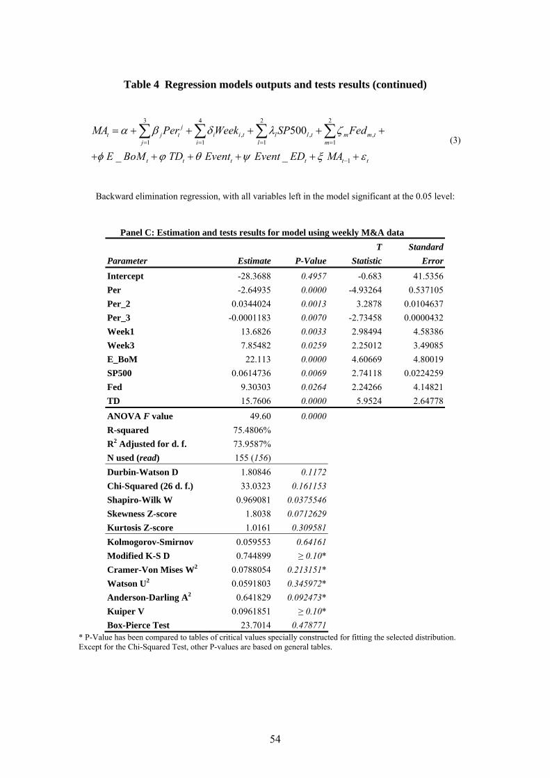
Table 4 Regression models outputs and tests results (continued)

3 4 2 2

, ,1 1 1 1

1

500

_ _

jt j t i i t l l t m

j i l m

t t t t t t

MA Per Week SP Fed

E BoM TD Event Event ED MA

α β δ λ ζ

φ ϕ θ ψ ξ= = = =

−

= + + + + +

+ + + + + +

∑ ∑ ∑ ∑ ,m t

ε (3)

Backward elimination regression, with all variables left in the model significant at the 0.05 level:

Panel C: Estimation and tests results for model using weekly M&A data T Standard Parameter Estimate P-Value Statistic Error

Intercept -28.3688 0.4957 -0.683 41.5356 Per -2.64935 0.0000 -4.93264 0.537105 Per_2 0.0344024 0.0013 3.2878 0.0104637 Per_3 -0.0001183 0.0070 -2.73458 0.0000432 Week1 13.6826 0.0033 2.98494 4.58386 Week3 7.85482 0.0259 2.25012 3.49085 E_BoM 22.113 0.0000 4.60669 4.80019 SP500 0.0614736 0.0069 2.74118 0.0224259 Fed 9.30303 0.0264 2.24266 4.14821 TD 15.7606 0.0000 5.9524 2.64778

ANOVA F value 49.60 0.0000 R-squared 75.4806% R2 Adjusted for d. f. 73.9587% N used (read) 155 (156) Durbin-Watson D 1.80846 0.1172 Chi-Squared (26 d. f.) 33.0323 0.161153 Shapiro-Wilk W 0.969081 0.0375546 Skewness Z-score 1.8038 0.0712629 Kurtosis Z-score 1.0161 0.309581 Kolmogorov-Smirnov 0.059553 0.64161 Modified K-S D 0.744899 ≥ 0.10* Cramer-Von Mises W2 0.0788054 0.213151* Watson U2 0.0591803 0.345972* Anderson-Darling A2 0.641829 0.092473* Kuiper V 0.0961851 ≥ 0.10* Box-Pierce Test 23.7014 0.478771

* P-Value has been compared to tables of critical values specially constructed for fitting the selected distribution. Except for the Chi-Squared Test, other P-values are based on general tables.

54

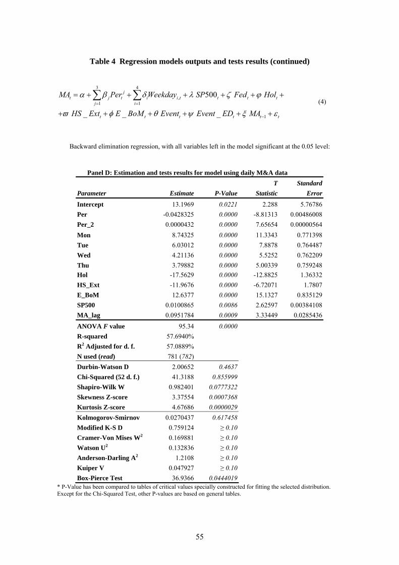
Table 4 Regression models outputs and tests results (continued)

3 4

,1 1

1

500

_ _ _

jt j t i i t t t

j i

t t t t t

t

t

MA Per Weekday SP Fed Hol

HS Ext E BoM Event Event ED MA

α β δ λ ζ ϕ

ϖ φ θ ψ ξ= =

−

= + + + + + +

+ + + + +

∑ ∑ε+

(4)

Backward elimination regression, with all variables left in the model significant at the 0.05 level:

Panel D: Estimation and tests results for model using daily M&A data T Standard Parameter Estimate P-Value Statistic Error

Intercept 13.1969 0.0221 2.288 5.76786 Per -0.0428325 0.0000 -8.81313 0.00486008 Per_2 0.0000432 0.0000 7.65654 0.00000564 Mon 8.74325 0.0000 11.3343 0.771398 Tue 6.03012 0.0000 7.8878 0.764487 Wed 4.21136 0.0000 5.5252 0.762209 Thu 3.79882 0.0000 5.00339 0.759248 Hol -17.5629 0.0000 -12.8825 1.36332 HS_Ext -11.9676 0.0000 -6.72071 1.7807 E_BoM 12.6377 0.0000 15.1327 0.835129 SP500 0.0100865 0.0086 2.62597 0.00384108 MA_lag 0.0951784 0.0009 3.33449 0.0285436

ANOVA F value 95.34 0.0000 R-squared 57.6940% R2 Adjusted for d. f. 57.0889% N used (read) 781 (782) Durbin-Watson D 2.00652 0.4637 Chi-Squared (52 d. f.) 41.3188 0.855999 Shapiro-Wilk W 0.982401 0.0777322 Skewness Z-score 3.37554 0.0007368 Kurtosis Z-score 4.67686 0.0000029 Kolmogorov-Smirnov 0.0270437 0.617458 Modified K-S D 0.759124 ≥ 0.10 Cramer-Von Mises W2 0.169881 ≥ 0.10 Watson U2 0.132836 ≥ 0.10 Anderson-Darling A2 1.2108 ≥ 0.10 Kuiper V 0.047927 ≥ 0.10 Box-Pierce Test 36.9366 0.0444019

* P-Value has been compared to tables of critical values specially constructed for fitting the selected distribution. Except for the Chi-Squared Test, other P-values are based on general tables.

55

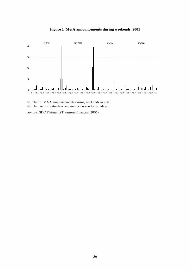
Figure 1 M&A announcements during weekends, 2001

0

10

20

30

40

67676767676767676767676767676767676767676767676767676767676767676767676767676767676767676767676767676767

1Q 2001 2Q 2001 3Q 2001 4Q 2001

Number of M&A announcements during weekends in 2001 Number six for Saturdays and number seven for Sundays.

Source: SDC Platinum (Thomson Financial, 2006).

56