The 1-D Heat Equation

18.303 Linear Partial Differential Equations

Matthew J. Hancock

Fall 2004

1 The 1-D Heat Equation

1.1 Physical derivation

Reference: Haberman §1.1-1.3

[Sept. 8, 2004]

In a metal rod with non-uniform temperature, heat (thermal energy) is transferred

from regions of higher temperature to regions of lower temperature. Three physical

principles are used here.

1. Heat (or thermal) energy of a body with uniform properties:

Heat energy = cmu,

where m is the body mass, u is the temperature, c is the specific heat, units [c] =

L2T −2U −1 (basic units are M mass, L length, T time, U temperature). c is the energy

required to raise a unit mass of the substance 1 unit in temperature.

2. Fourier’s law of heat transfer: rate of heat transfer proportional to negative

temperature gradient,

Rate of heat transfer ∂u = −K0 (1)

area ∂x

where K0 is the thermal conductivity, units [K0] = MLT −3 U −1 . In other words, heat

is transferred from areas of high temp to low temp.

3. Conservation of energy.

Consider a uniform rod of length l with non-uniform temperature lying on the

x-axis from x = 0 to x = L. By uniform rod, we mean the density ρ, specific heat

c, thermal conductivity K0, cross-sectional area A are ALL constant. Assume the

1

� � � �

� � � � � �

sides of the rod are insulated and only the ends may be exposed. Also assume there

is no heat source within the rod. Consider an arbitrary thin segment of the rod thin

slice of the rod of width ∆x between x and x + ∆x. The slice is so thin that the

temperature throughout it is u (x, t). Thus,

Heat energy of segment = c × ρA∆x × u = cρA∆xu (x, t) .

By conservation of energy,

change of heat in from heat out from

heat energy of = − . left boundary right boundary

segment in time ∆t

From Fourier’s Law (1),

∂u ∂u cρA∆xu (x, t + ∆t) − cρA∆xu (x, t) = ∆tA −K0 − ∆tA −K0

∂x ∂x x x+∆x

Rearranging yields (recall ρ, c, A, K0 are constant),

u (x, t + ∆t) − u (x, t) K0 ∂u − ∂u ∂x x+∆x ∂x x =

∆t cρ ∆x

Taking the limit ∆t, ∆x → 0 gives the Heat Equation,

∂u ∂2u = κ (2)

∂t ∂x2

where K0

κ = (3)cρ

is called the thermal diffusivity, units [κ] = L2/T . Since the slice was chosen arbi-

trarily, the Heat Equation (2) applies throughout the rod.

1.2 Initial condition and boundary conditions

To make use of the Heat Equation, we need more information:

1. Initial Condition (IC): in this case, the initial temperature distribution in the

rod u (x, 0).

2. Boundary Conditions (BC): in this case, the temperature of the rod is affected

by what happens at the ends, x = 0, l. What happens to the temperature at the

end of the rod must be specified. In reality, the BCs can be complicated. Here we

consider three simple cases for the boundary at x = 0.

2

� �

(a) Temperature prescribed at a boundary. For t > 0,

u (0, t) = u1 (t) .

(b) Insulated boundary. The heat flow can be prescribed at the boundaries,

∂u −K0 (0, t) = φ1 (t)∂x

(c) Mixed condition: an equation involving u (0, t), ∂u/∂x (0, t), etc.

Example 1. Consider a rod of length l with insulated sides is given an initial

temperature distribution of f (x) degree C, for 0 < x < l. Find u (x, t) at subsequent

times t > 0 if end of rod are kept at 0o C.

The Heat Eqn and corresponding IC and BCs are thus

PDE: ut = κuxx, 0 < x < l, (4)

IC: u (x, 0) = f (x) , 0 < x < l, (5)

BC: u (0, t) = u (L, t) = 0, t > 0. (6)

Physical intuition: we expect u → 0 as t → ∞.

1.3 Non-dimensionalization

Dimensional (or physical) terms in the PDE (2): k, l. Others could be introduced in

IC and BCs. To make life easier, we try and group as many of these physical constants

as we can and eliminate them from as many places in the problem as possible. For

instance, in Example 1, we can non-dimensionalize (or scale or normalize) x by the

length of the rod l, x

x = , t = c1t. (7)l

The variables x, t are dimensionless (i.e. no units, [x] = 1). While x is in the range

x is in the range 0 < ˆ0 < x < l, ˆ x < 1. The constant c1, with units 1/T , is to be

determined.

The choice of dimensionless variables is an ART. Sometimes the statement of the

problem gives hints: e.g. the length l of the rod (1 is nicer to deal with than l, an

unspecified quantity). Often you have to solve the problem first, look at the solution,

and try to simplify the notation.

We define new u and f in terms of the new variables,

u ˆ x) = f (x) . (8)ˆ x, t = u (x, t) , f (ˆ

3

� � � �

� �

From the chain rule,

u u∂u ∂ˆ ∂t ∂ˆut = = ,

∂t ∂t ∂t = c1

∂tu x u∂u ∂ˆ ∂ˆ 1 ∂ˆ

ux = = = x x∂x ∂ˆ ∂x l ∂ˆ

1 ∂2

uu

xx = l2 ∂ˆ2x

Substituting these into the Heat Eqn (4) gives

u u∂ˆ κ ∂2

ut = kuxx ⇒ c1 = l2 ∂ˆ2∂t x

To make the PDE simpler, we choose c1 = κ/l2, so that

∂ˆ ∂2 u u

∂t=

∂ˆ2 , 0 < x < 1,

x

Remember to also scale the IC (5) and BC (6):

ˆ x, 0) = f (ˆ x < 1,IC: u (ˆ x) , 0 < ˆ

BC: u 0, t = ˆ ˆˆ u 1, t = 0, t > 0.

Note that to keep things simple we have not scaled u. Exercise: check that if we had

set

ˆ ˆ x) = c2f (x) ,

c

u x, t = c2u (x, t) , f (ˆ

2 would cancel from the PDE, IC and BC. We may therefore assume that u and f

are also dimensionless.

1.4 Dimensionless problem

[Sept. 10, 2004]

Dropping hats, we have the dimensionless problem

PDE: ut = uxx, 0 < x < 1, (9)

IC: u (x, 0) = f (x) , 0 < x < 1, (10)

BC: u (0, t) = u (1, t) = 0, t > 0, (11)

where x, t are dimensionless scalings of physical position and time.

4

2 Separation of variables

Ref: Haberman, §2.1-2.3

We look for a solution to the dimensionless Heat Equation (9) – (11) of the form

u (x, t) = X (x) T (t) (12)

Take the relevant partial derivatives:

uxx = X ′′ (x) T (t) , ut = X (x) T ′ (t)

u

where primes denote differentiation of a single-variable function. The PDE (9), ut =

xx, becomes T ′ (t) X ′′ (x)

= T (t) X (x)

The left hand side (l.h.s.) depends only on t and the right hand side (r.h.s.) only

depends on x. Hence if t varies and x is held fixed, the r.h.s. is constant, and hence

T ′/T must also be constant, which we set to −λ by convention:

X ′′ (x)T ′ (t) = = −λ, λ = constant. (13)

T (t) X (x)

The BCs become, for t > 0,

u (0, t) = X (0) T (t) = 0

u (1, t) = X (1) T (t) = 0

Taking T (t) = 0 would give u = 0 for all time and space (called the trivial solution),

from (12), which does not satisfy the IC unless f (x) = 0. If you are lucky and

f (x) = 0, then u = 0 is the solution (this has to do with uniqueness of the solution,

which we’ll come back to). If f (x) is not zero for all 0 < x < 1, then T (t) cannot be

zero and hence the above equations are only satisfied if

X (0) = X (1) = 0. (14)

2.1 Solving for X (x)

We obtain a boundary value problem for X (x), from (13) and (14),

X ′′ (x) + λX (x) = 0, 0 < x < 1, (15)

X (0) = X (1) = 0. (16)

5

� �

′′

This is an example of a Sturm-Liouville problem (from your ODEs class).

There are 3 cases: λ > 0, λ < 0 and λ = 0.

(i) λ < 0. Let λ = −k2 < 0. Then the solution to (15) is

X = Aekx + Be−kx

for integration constants A, B found from imposing the BCs (16),

X (0) = A + B = 0, X (1) = Aek + Be−k = 0.

The first gives A = −B, the second then gives A e2k − 1 = 0, and since |k| > 0 we

have A = B = u = 0, which is the trivial solution. Thus we discard the case λ < 0.

(ii) λ = 0. Then X (x) = Ax + B and the BCs imply 0 = X (0) = B, 0 = X (1) =

A, so that A = B = u = 0. We discard this case also.

(iii) λ > 0. In this case, (15) becomes

X (x) + k2X (x) = 0,

the simple harmonic equation, whose solution is �√ � �√ � X (x) = A cos λx + B sin λx (17)

√ The BCs imply 0 = X (0) = A, and B sin λ = 0. We don’t want B = 0, since that

would give the trivial solution u = 0, so we must have √

sin λ = 0. (18) √

Thus λ = nπ, for any nonzero integer n, and gives a solution (since A = 0),

Xn (x) = bn sin (nπx) , n = 1, 2, 3, ... (19)

We have assumed that n > 0, since n < 0 gives the same solution as n > 0.

The Xn (x) are the eigenfunctions of the Sturm-Liouville problem (15) with eigen-

values λn = n2π2 for n = 1, 2, 3, ....

2.2 Solving for T (t)

When solving for X (x), we found that non-trivial solutions arose for λ = n2π2 for all

nonzero integers n. The equation for T (t) is thus, from (13),

T ′ (t) = −n 2π2T (t)

and, for n, the solution is

Tn = cne −n2π2t , n = 1, 2, 3, ... (20)

where the cn’s are constants of integration.

6

�

� �

�

u

2.3 Full solution u (x, t)

Putting things together, we have, from (12), (19) and (20),

n (x, t) = Bn sin (nπx) e −n2π2t , n = 1, 2, 3, ... (21)

where Bn = cnbn. Each function un (x, t) is a solution to the PDE (9) and the BCs

(11). But, in general, they will not individually satisfy the IC (10),

un (x, 0) = Bn sin (nπx) = f (x) .

We now apply the principle of superposition: if u1 and u2 are two solutions to the

PDE (9) and BC (11), then c1u1 + c2u2 is also a solution, for any constants c1, c2.

This relies on the linearity of the PDE and BCs. We will, of course, soon make this

more precise....

Since each un (x, 0) is a solution of the PDE, then the principle of superposition

says any finite sum is also a solution. To solve the IC, we will probably need all the

solutions un, and form the infinite sum (convergence properties to be checked),

∞

u (x, t) = un (x, t) . (22) n=1

u (x, t) satisfies the BCs (11) since each un (x, t) does. Assuming term-by-term dif-

ferentiation holds (to be checked) for the infinite sum, then u (x, t) also satisfies the

PDE (9). To satisfy the IC, we need to find Bn’s such that

∞ ∞

f (x) = u (x, 0) = un (x, 0) = Bn sin (nπx) . (23) n=1 n=1

This is the Fourier Sine Series of f (x).

To solve for the Bn’s, we use the orthogonality property for the eigenfunctions

sin (nπx), � 1 0 m �= n sin (mπx) sin (nπx) dx = (24)

0 1/2 m = n

Multiplying both sides of (23) by sin (mπx) and integrating from 0 to 1 gives

∞� 1 � � 1

sin (mπx) f (x) dx = Bn sin (nπx) sin (mπx) dx 0 n=1 0

Using (24) yields � 1

Bm = 2 sin (mπx) f (x) dx (25) 0

7

�

�

�

�

�

The full solution is, from (21) and (22),∞

u (x, t) = Bn sin (nπx) e −n2π2t , (26) n=1

where Bn are given by (25).

To derive the solution (26) of the Heat Equation (9) and corresponding BCs

(11) and IC (10), we used properties of linear operators and infinite series that need

justification.

3 Uniform convergence, differentiation and inte-

gration of an infinite series

[Sept 13, 2004]

The infinite series solution (26) to the Heat Equation (9) only makes sense if it

converges uniformly1 on the interval [0, 1]. The reason is that to satisfy the PDE,

we must be able to integrate and differentiate the infinite series term-by-term. This

can only be done if the infinite series AND its derivatives converge uniformly. The

following results2 dictate when we can differentiate and integrate an infinite series

term-by-term.

Theorem [Term-by-term differentiation] If, on an interval3 x ∈ [a, b], ∞

1. f (x) = fn (x) converges uniformly, n=1

∞

2. f ′ n (x) converges uniformly, n=1

3. f ′ n (x) are continuous,

then the series may be differentiated term-by-term, ∞

f ′ (x) = f ′ n (x) . n=1

Theorem [Term-by-term integration] If, on an interval x ∈ [a, b], ∞

1. f (x) = fn (x) converges uniformly, n=1

1The precise definitions are outlined in §3.3 (optional reading). 2Proofs of these theorems [optional reading] can be found in any good text on real analysis [e.g.

Rudin] - start by reading §3.3. 3Note that the symbol ∈ means “an element of”. So x ∈ [0, l] means x is in the interval [0, l].

8

�

3. f ′ n (x) are integrable,

then the series may be integrated term-by-term, � b ∞ � b

f (x) dx = fn (x) dx. a n=1 a

Thus, uniform convergence of an infinite series of functions is an important prop-

erty. To check that an infinite series has this property, we use the following tests in

succession (examples to follow):

Theorem [Weirstrass M-Test for uniform convergence of a series of functions]

Suppose {fn (x)}∞ is a sequence of functions defined on a subset E ⊆ R, and n=1

suppose

|fn (x)| ≤ Mn (x ∈ E, n = 1, 2, 3, ...).

Then the series of functions �∞ fn (x) converges uniformly on E if the series of n=1 �∞numbers n=1 Mn converges absolutely.

Theorem [Ratio Test for convergence of a series of numbers] The series �∞

n=1 an

converges absolutely if the ratio of successive terms is less than a constant r < 1, i.e.

|an+1| ≤ r < 1, (27)|an| for all n ≥ N ≥ 1.

Note: the N is here to allow for the first N − 1 terms in the series not obeying

the ratio rule (27).

3.1 Examples for the Ratio Test

E.g. Consider the infinite series of numbers ∞ � �� 1 n

(28)2

n=1

Writing this as a series �∞ an, we identify an = (1/2)n . We form the ratio of n=1

successive elements in the series,

|an+1| (1/2)n+1 1 = = < 1 |an| (1/2)n 2

Thus, the infinite series (28) satisfies the requirements of the Ratio Test with r = 1/2,

and hence (28) converges absolutely.

E.g. Consider the infinite series ∞ � 1

(29) n

n=1

9

� �

�∞Writing this as a series an, we identify an = 1/n. We form the ratio of successive n=1

elements in the series, |an+1| 1/ (n + 1) n

= = |an| 1/n n + 1 nNote that limn→∞ n+1 = 1, and hence there is no upper bound r < 1 that is greater

than |an+1| / |an| for ALL n. So the Ratio Test fails, i.e. it gives no information. It

turns out that this series diverges, i.e. the sum is infinite.

E.g. Consider the infinite series

∞ � 1 (30)

n2 n=1 �∞Again, writing this as a series an, we identify an = 1/n2 . We form the ratio of n=1

successive elements in the series,

2|an+1| 1/ (n + 1)2 n= = 2|an| 1/n2 (n + 1)

2nNote again that limn→∞ (n+1)2 = 1, and hence there is no r < 1 that is greater than

|an+1| / |an| for ALL n. So the Ratio Test gives no information again. However, it

turns out that this series converges:

∞ � 1 π2

= n2 6

n=1

So the fact that the Ratio Test fails does not imply anything about the convergence

of the series!

Note that the infinite series ∞ � 1 (31)

np n=1

converges for p > 1 and diverges (is infinite) for p ≤ 1.

3.2 Application to the solution of the Heat Equation

[Sept 15, 2004]

We now use the Weirstrass M-Test and the Ratio Test to show that the infinite

series solution (26) to the Heat Equation converges uniformly,

∞ ∞

u (x, t) = un (x, t) = Bn sin (nπx) e −n2π2t , (32) n=1 n=1

for all positive time, i.e. t ≥ t0 > 0, and space x ∈ [0, 1], provided the initial condition

f (x) is piecewise continuous.

10

� �

� � � � � �

� � � � � �

� �

�

To apply the M-Test, we need bounds on |un (x, t)|, � −n2π2t0|un (x, t)| = � Bn sin (nπx) e −n2π2t�� ≤ |Bn| e , for all x ∈ [0, 1] . (33)

We now need a bound on the Fourier coefficients |Bn|. Note that from Eq. (25), � 1 � 1� 1

|Bm| = �2 sin (mπx) f (x) dx� ≤ 2 |sin (mπx) f (x)| dx ≤ 2 |f (x)| dx, (34) 0 0 0

for all x ∈ [0, 1]. To obtain the inequality (34), we used the fact that |sin (mπx)| ≤ 1

and, for any integrable function h (x),

� b � b � h (x) dx� ≤ |h (x)| dx. a a

You’ve seen this integral inequality, I hope, in past Calculus classes. We combine (33)

and (34), to obtain

|un (x, t)| ≤ Mn (35)

where � 1

Mn = 2 |f (x)| dx e −n2π2t0 . 0

To apply the Weirstrass M-Test, we first need to show that the infinite series of �∞numbers n=1 Mn converges absolutely (we will use the Ratio Test). Forming the

ratio of successive terms yields

Mn+1 e−(n+1)2π2t0

= e(n2−(n+1)2)π2t0 −(2n+1)π2t0 ≤ e −π2t0 < 1,= = e n = 1, 2, 3, ... Mn e−n2π2t0

Thus, by the Ratio Test with r = e−π2t0 < 1, the sum

∞

Mn

n=1

converges absolutely, and hence by Eq. (33) and the Weirstrass M-Test, �∞ un (x, t)n=1

converges uniformly for x ∈ [0, 1] and t ≥ t0 > 0.

A similar argument holds for the convergence of the derivatives ut and uxx. Thus,

for all t ≥ t0 > 0, the infinite series (32) for u may be differentiated term-by-term

and since each un (x, t) satisfies the PDE and BCs, then so does u (x, t). Later, after

considering properties of Fourier Series, we will show that u converges even at t = 0

(given conditions on the initial condition f (x)).

11

� � � � � � �

�

�

3.3 Background [optional]

[Note: You are not responsible for the material in this subsection 3.3 - it is only added

for completeness]

Ref: Chapters 3 & 7 of “Principles of Mathematical Analysis”, W. Rudin, McGraw-

Hill, 1976.

Definition Convergence of a series of numbers: the series of real numbers �∞ ann=1

converges if for every ε > 0, there is an integer N such that for any n ≥ N ,

� ∞ � � am� < ε. m=n

Definition Absolute convergence of a series of numbers: the series of real numbers �∞ �∞ an is said to converge absolutely if the series |an| converges. n=1 n=1

Definition Uniform convergence of a sequence of functions: A sequence of func-

tions {fn (x)}∞ defined on a subset E ⊆ R converges uniformly on E to a function n=1

f (x) if for every ε > 0 there is an integer N such that for any n ≥ N ,

|fn (x) − f (x)| < ε

for all x ∈ E.

Note: pointwise convergence does not imply uniform convergence, i.e. in the

definition, for each ε, one N works for all x in E. For example, consider the sequence nof functions {x }∞ on the interval [0, 1]. These converge pointwise to the function n=1

0, 0 ≤ x < 1,f (x) =

1, x = 1

on [0, 1], but do not converge uniformly.

Definition Uniform convergence of a series of functions: A series of functions �∞ fn (x) defined on a subset E ⊆ R converges uniformly on E to a function g (x)n=1

if the partial sums m

sm (x) = fn (x) n=1

converge uniformly to g (x) on E.

12

� �

4 Linearity, Homogeneity, and Superposition

Definition Linear space: A set V is a linear space if, for any two elements v1, v2 ∈ V

and any scalar (i.e. number) k ∈ R, the terms v1 + v2 and kv1 are also elements of V.

E.g. Let S denote the set of C2 (twice-continuously differentiable in x and t)

functions f (x, t) for x ∈ [0, 1], t ≥ 0. We write S as

S = f (x, t) | f (x, t) is C2 for x ∈ [0, 1] , t ≥ 0

If f1, f2 ∈ S, i.e. f1, f2 are functions that have continuous second derivatives in space

and time, and k ∈ R, then f1 + f2 and kf1 also have continuous second derivatives,

and hence are both elements of S. Thus, by definition, S forms a linear space over

the real numbers R. For instance, f1 (x, t) = sin (πx) e−π2t and f2 = x2 + t3 .

Definition Linear operator: An operator L : V → W is linear if

L (v1 + v2) = L (v1) + L (v2) , (36)

L (kv1) = kL (v1) , (37)

for all v1, v2 ∈ V, k ∈ R. The first property is the summation property; the second is

the scalar multiplication property.

The term “operator” is very general. It could be a linear transformation of vectors

in a vector space, or the derivative operation ∂/∂x acting on functions. Differential

operators are just operators that contain derivatives. So ∂/∂x and ∂/∂x + ∂/∂y are

differential operators. These operators are functions that act on other functions. For

example, the x-derivative operation is linear on a space of functions, even though the

functions the derivative acts on might not be linear in x:

∂ � 2 � ∂ ∂ � �

cos x + x = (cos x) + x 2 . ∂x ∂x ∂x

E.g. the identity operator I, which maps each element to itself, i.e. for all elements

v ∈ V we have I (v) = v. Check for yourself that I satisfies (36) and (37) for an

arbitrary linear space V.

E.g. consider the partial derivative operator acting on S,

∂u D (u) = , u ∈ S. ∂x

From the well-known properties of the derivative, namely

∂ ∂u ∂v (u + v) = + , u, v ∈ S,

∂x ∂x ∂x

∂ ∂u (ku) = k , u ∈ S, k ∈ R

∂x ∂x

13

it follows that the operator D satisfies properties (36) and (37) and is therefore a

linear operator.

E.g. Consider the operator that defines the Heat Equation

∂ ∂2

L = − ∂t ∂x2

and acts over the linear space S of C2 functions. The Heat Equation can be written

as ∂u ∂2 u

L (u) = − = 0. ∂t ∂x2

For any two functions u, v ∈ S and a real k ∈ R, � ∂2 �

∂ L (u + v) = − (u + v)

∂t ∂x2

∂ ∂2 ∂u ∂2u ∂v ∂2 v = (u + v) −

∂x2 (u + v) = − + − = L (u) + L (v)

∂t ∂t ∂x2 ∂t ∂x2 � ∂2 �

∂ ∂ ∂2 � ∂u ∂2u

�

L (ku) = ∂t

− ∂x2

(ku) = (ku) − ∂x2

(ku) = k − = kL (u)∂t ∂t ∂x2

Thus, L satisfies properties (36) and (37) and is therefore a linear operator.

4.1 Linear and homogeneous PDE, BC, IC

Consider a differential operator L and operators B1, B2, I that define the following

problem:

PDE: L (u) = h (x, t) , with

BC: B1 (u (0, t)) = g1 (t) , B2 (u (1, t)) = g2 (t)

IC: I (u (x, 0)) = f (x) .

Definition The PDE is linear if the operator L is linear.

Definition The PDE is homogeneous if h (x, t) = 0.

Definition The BCs are linear if B1, B2 are linear. The BCs are homogeneous if

g1 (t) = g2 (t) = 0.

Definition The IC is linear if I is a linear. The IC is homogeneous if f (x) = 0.

14

4.2 The Principle of Superposition

[Sept 17, 2004]

The Principle of Superposition has three parts, all which follow from the definition

of a linear operator:

(1) If L (u) = 0 is a linear, homogeneous PDE and u1, u2 are solutions, then

c1u1 + c2u2 is also a solution, for all c1, c2 ∈ R.

(2) If u1 is a solution to L (u1) = f1, u2 is a solution to L (u2) = f2, and L is

linear, then c1u1 + c2u2 is a solution to

L (u) = c1f1 + c2f2,

for all c1, c2 ∈ R.

(3) If a PDE, its BCs, and its IC are all linear, then solutions can be superposed

in a manner similar to (1) and (2).

E.g. Suppose u1 is a solution to

BB

L (u) = ut − uxx = 0

1 (u (0, t)) = u (0, t) = 0

2 (u (1, t)) = u (1, t) = 0

I (u (x, 0)) = u (x, 0) = 100

and u2 is a solution to

BB

L (u) = ut − uxx = 0

1 (u (0, t)) = u (0, t) = 100

2 (u (1, t)) = u (1, t) = 0

I (u (x, 0)) = u (x, 0) = 0

Then 2u1 − u2 would solve

BB

L (u) = ut − uxx = 0

1 (u (0, t)) = u (0, t) = −100

2 (u (1, t)) = u (1, t) = 0

I (u (x, 0)) = u (x, 0) = 200

Keep in mind that to solve L (u) = g with inhomogeneous BCs using superposition,

we need to solve two problems: L (u) = g with homogeneous BCs and L (u) = 0 with

inhomogeneous BCs.

15

�

�

� �

4.3 Application to the solution of the Heat Equation

Recall that we showed that un (x, t) satisfied the PDE and BCs. Since the PDE (9)

and BCs (11) are linear and homogeneous, then we apply the Principle of Superposi-

tion (1) repeatedly to find that the infinite sum u (x, t) given in (32) is also a solution,

provided of course that it can be differentiated term-by-term.

5 Example : Cooling of a rod from a constant ini-

tial temperature

Ref: §2.3.7 Haberman

Suppose the initial temperature distribution f (x) in the rod is constant, i.e.

f (x) = u0. The solution for the temperature in the rod is (26),

∞

u (x, t) = Bn sin (nπx) e −n2π2t , n=1

where, from (25), the Fourier coefficients are given by � 1

B

� 1

n = 2 sin (nπx) f (x) dx = 2u0 sin (nπx) dx. 0 0

Calculating the integrals gives

� 1 cos (nπ) − 1 2u0 0 n even Bn = 2u0 sin (nπx) dx = −2u0 = − ((−1)n − 1) =

4u0 0 nπ nπ

nπ n odd

In other words, 4u0

B2n = 0, B2n−1 = (2n − 1) π

and the solution becomes

∞ � sin ((2n − 1) πx) � � u (x, t) =

4u0 exp − (2n − 1)2 π2t . (38)

π (2n − 1)n=1

5.1 Approximate form of solution

The number of terms of the series (38) needed to get a good approximation for u (x, t)

depends on how close t is to 0. The series is

4u0 −9π2t u (x, t) = sin (πx) e −π2t + sin (3πx)

e + · · · . π 3

16

The ratio of the first and second terms is

|second term| e−8π2t |sin 3πx|= |first term| 3 |sin πx| ≤ e −8π2t using |sin nx| ≤ n |sin x|

1 ≤ e −8 for t ≥ π2

< 0.00034

It can also be shown that the first term dominates the sum of the rest of the terms,

and hence 1

u (x, t) ≈ 4u0

sin (πx) e −π2t , for t ≥ . (39)π π2

κWhat does t = 1/π2 correspond to in physical time? In physical time t′ = l2 t (recall

our scaling - here we use t as the dimensionless time and t′ as dimensional time),

t = 1/π2 corresponds to:

t

t

t′ ≈ 15 minutes, for a 1 m rod of copper (κ ≈ 1.1 cm2 sec−1) ′ ≈ 169 minutes, for a 1 m rod of steel (κ ≈ 0.1 cm2 sec−1) ′ ≈ 47 hours, for a 1 m rod of glass (κ ≈ 0.006 cm2 sec−1 )

At t = 1/π2, the temperature at the center of the rod (x = 1/2) is, from (39),

4 u (x, t) ≈ u0 = 0.47u0.

πe

Thus, after a (scaled) time t = 1/π2, the temperature has decreased by a factor of

0.47 from the initial temperature u0.

5.2 Geometrical visualization of the solution

[Sept 20, 2004]

To analyze qualitative features of the solution, we draw various types of curves in

2D:

1. Spatial temperature profile, given by

u = u (x, t0)

where t0 is a fixed value of x. These profiles are curves in the ux-plane.

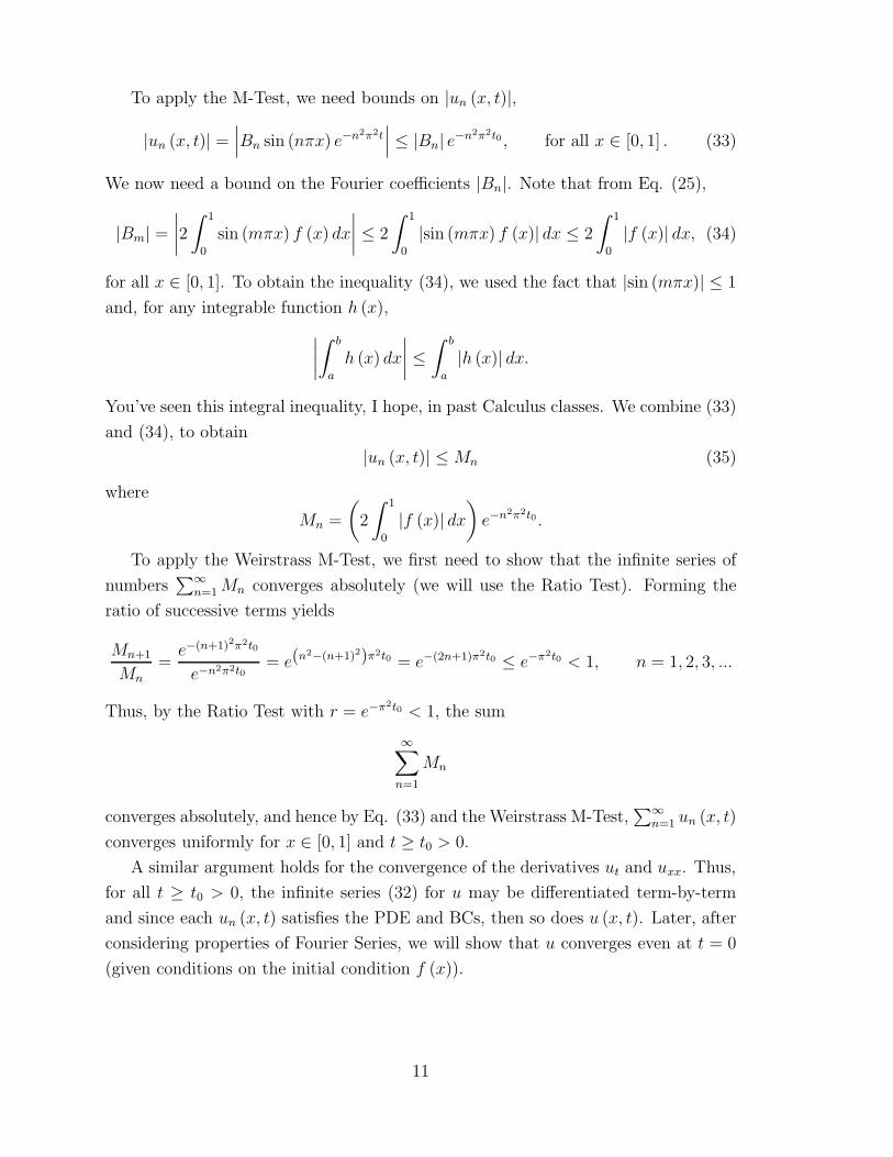
2. Temperature profiles in time,

u = u (x0, t)

where x0 is a fixed value of x. These profiles are curves in the ut-plane.

17

Figure 1: Spatial temperature profiles u(x, t0).

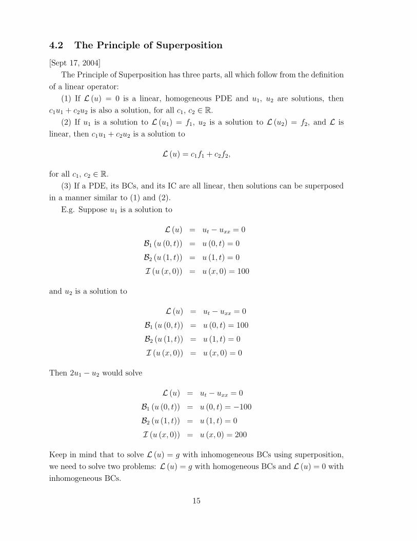
3. Curves of constant temperature in the xt-plane (level curves),

u (x, t) = C

where C is a constant.

Note that the solution u = u (x, t) is a 2D surface in the 3D uxt-space. The above

families of curves are the different cross-sections of this solution surface. Drawing the

2D cross-sections is much simpler than drawing the 3D solution surface.

Sketch typical curves: when sketching the curves in 1-3 above, we draw a few

typical curves and any special cases. While math packages such as Matlab can be

used to compute the curves from, say, 20 terms in the full power series solution (38),

the emphasis in this course is to use simple considerations to get a rough idea of what

the solution looks like. For example, one can use the first term approximation (39),

simple physical considerations on heat transfer, and the fact that the solution u (x, t)

is continuous in x and t, so that if t1 is close to t1, u (x, t1) is close to u (x, t2).

18

� � � �

� � �

� �

5.2.1 Spatial temperature profiles

For fixed t = t0, the approximate solution (39),

u (x, t) ≈ 4u0

e −π2t0 sin (πx) , t ≥ 1/π2 . π

This suggests the center of the rod, x = 1/2, is a line of symmetry for u (x, t), i.e.

1 1 u + s, t = u − s, t

2 2

and, for each fixed time, the location of the maximum temperature (provided u0 >

0). We can prove the symmetry property by noting that the original PDE/BC/IC

problem is invariant under the transformation x → 1 − x. Note also that, from (38), ∞

ux (x, t) = 4u0 cos ((2n − 1) πx) exp − (2n − 1)2 π2t n=1

Thus ux (1/2, t) = 0 and uxx (1/2, t) < 0, so the 2nd derivative test implies that

x = 1/2 is a local max.

In Figure 1, we have plotted two typical profiles, one at early times t = t0 ≈ 0 and

the other at late times t = t0 � 0, and one special profile, the initial temperature

at t = 0 (u = u0). The profile for t = t0 � 0 is found from the approximation

u ≈ (constant) sin πx. Note that the linear x = 1/2 is a line of symmetry.

5.2.2 Temperature profiles in time

Setting x = x0 in the approximate solution (39),

u (x0, t) ≈ 4u0

sin (πx0) e −π2t , t ≥ 1/π2 . π

Two typical profiles are sketched in Figure 2, one near the center of the rod (x0 ≈ 1/2)

and one near the edges (x0 ≈ 0 or 1). To draw these we noted that the center of

the rod cools more slowly than points near the ends. One special profile is plotted,

namely the temperature at the rod ends (x = 0, 1).

5.2.3 Curves of constant temperature (level curves of u(x, t))

In Figure 3, we have drawn three typical level curves and two special ones, u = 0 (rod

ends) and u = u0 (the initial condition). For a fixed x = x0, the temperature in the

rod decreases as t increases (motivated by the approximate solution), as indicated by

the points of intersection on the dashed line. The center of the rod (x = 1/2) is a

line of symmetry, and at any time, the maximum temperature is at the center. Note

that at t = 0, the temperature is discontinuous at x = 0, 1.

When drawing visualization curves, the following result is helpful.

19

Figure 2: Temperature profiles in time u (x0, t).

Figure 3: Curves of constant temperature u(x, t) = c, i.e., the level curves of u(x, t).

20

′′

5.2.4 Maximum Principle for the basic Heat Problem

This result is useful when plotting solutions: the extrema of the solution of the

heat equation occurs on the space-time “boundary”, i.e. the maximum of the initial

condition and of the time-varying boundary conditions. More precisely, given the

heat equation with some initial condition f (x) and BCs u (0, t), u (1, t), then on a

given time interval [0, T ], the solution u (x, t) is bounded by

umin ≤ u (x, t) ≤ umax

where � �

umax = max max 0<x<1

f (x) , max 0<t<T

u (0, t) , max 0<t<T

u (1, t) � �

umin = min min 0<x<1

f (x) , min 0<t<T

u (0, t) , min 0<t<T

u (1, t)

Thus, in the example above, umin = 0 and umax = u0, hence for all x ∈ [0, 1] and

t ∈ [0, T ], 0 ≤ u (x, t) ≤ u0.

6 Asymptotic (long time) behavior and the steady-

state

Intuition tells us that if the ends of the rod are held at 0o C and there are no heat

sources or sinks in the rod, the temperature in the rod will eventually reach 0. The

solution above confirms this. However, we do not have to solve the problem to

determine the asymptotic or long-time behavior of the solution.

Instead, the equilibrium or steady-state solution u = uE (x) must be independent

of time, and will thus satisfy the PDE and BCs with ut = 0,

uE = 0, 0 < x < 1; uE (0) = uE (1) = 0.

The solution is uE = c1x + c2 and imposing the BCs implies uE (x) = 0. In other

words, regardless of the initial temperature distribution u (x, 0) = f (x) in the rod,

the temperature eventually goes to zero.

6.1 Rate of decay of u (x, t)

How fast does u approach uE = 0? From our estimate (34) above,

2π2t|un (x, t)| ≤ Be−n , n = 1, 2, 3, ...

21

� �� � � � � � �

� � �

� � � � � � �

� � � �

�

� � �

n where B is a constant. Noting that e−n2π2t ≤ e−nπ2t = e−π2t , we have

� ∞ � ∞ ∞ � un (x, t)� ≤ |un (x, t)| ≤ B r n = Br

, r = e −π2t < 1 (t > 0). � � 1 − r n=1 n=1 n=1

rThe last step is the geometric series result �∞ rn =

1−r , for |r| < 1. Thus n=1

� ∞ � �� � Be−π2t � un (x, t) �� ≤ 1 − e−π2t

, t > 0. (40) n=1

Therefore

• u (x, t) approaches the steady-state uE (x) = 0 exponentially fast (i.e. the rod

cools quickly)

• the first term in the series, sin (πx) e−π2t (term with smallest eigenvalue λ = π)

determines the rate of decay of u (x, t)

• the Bn’s may also affect the rate of approach to the steady-state, for other

problems

6.2 Error of first-term approximation

Using the method in the previous section, we can compute the error between the

first-term and the full solution (38),

� ∞ � |u (x, t) − u1 (x, t)| = � un (x, t) − u1 (x, t)�

n=1 � ∞ � ∞ ∞ � � � Br2

= � un (x, t)� ≤ |un (x, t)| ≤ B r n = � � 1 − r n=2 n=2 n=2

where r = e−π2t . Hence the solution u (x, t) approaches the first term u1 (x, t) expo-

nentially fast, Be−2π2t

|u (x, t) − u1 (x, t)| ≤ 1 − e−π2t

, t > 0. (41)

With a little more work we can get a much tighter (i.e. better) upper bound. We

consider the sum ∞

|un (x, t)|n=N

Substituting for un (x, t) gives

∞ ∞ ∞

|un (x, t)| ≤ B e −n2π2t = Be−N 2π2t e −(n2−N 2)π2t (42) n=N n=N n=N

22

� �

�

� � � � � �

� � � �

� � � � � � � �

Here’s the trick: for n ≥ N ,

n 2 − N2 = (n + N) (n − N) ≥ 2N (n − N) ≥ 0.

Since e−x is a decreasing function, then

−(n2−N2)π2t ≤ e −2N(n−N)π2t (43)e

for t > 0. Using the inequality (43) in Eq. (42) gives

∞ ∞ −2N(n−N)π2t|un (x, t)| ≤ Be−N2π2t e

n=N n=N � �N ∞ � � e−2Nπ2t

= BeN2π2t e −2Nπ2tn

= BeN2π2t

1 − e−2Nπ2t .

n=N

Simplifying the expression on the right hand side yields

∞ � Be−N2π2t

|un (x, t)| ≤ (44)1 − e−2Nπ2t

n=N

For N = 1, (44) gives the temperature decay

� ∞ � ∞ � � Be−π2t

|u (x, t)| = � un (x, t)� ≤ |un (x, t)| ≤ 1 − e−2π2t

, (45) n=N n=N

which is slightly tighter than (40). For N = 2, (44) gives the error between u (x, t)

and the first term approximation,

� ∞ � ∞ � � Be−4π2t

|u (x, t) − u1 (x, t)| = � un (x, t)� ≤ |un (x, t)| ≤� � 1 − e−4π2t n=2 n=2

which is a much better upper bound than (41).

Note that for an initial condition u (x, 0) = f (x) that is is symmetric with respect

to x = 1/2 (e.g. f (x) = u0), then u2n = 0 for all n, and hence error between u (x, t)

and the first term u1 (x, t) is even smaller,

� ∞ � ∞

|u (x, t) − u1 (x, t)| = � un (x, t)� ≤ |un (x, t)|n=3 n=3

Applying result (44) with N = 3 gives

Be−9π2t

|u (x, t) − u1 (x, t)| ≤ 1 − e−6π2t

.

Thus, in this case, the error between the solution u (x, t) and the first term u1 (x, t)

decays as e−9π2t - very quickly!

23

�

�

�

�

7 Review of Fourier Series

Ref: Ch 3, Haberman

[Sept 22, 2004]

Motivation: Recall that the initial temperature distribution satisfies ∞

f (x) = u (x, 0) = Bn sin (nπx) . n=1

In the example above with a constant initial temperature distribution, f (x) = u0, we

have ∞4u0

� sin ((2n − 1) πx) u0 = . (46)

π 2n − 1 n=1

Note that at x = 0 and x = 1, the r.h.s. does NOT converge to u0 �= 0, but rather to

0 (the BCs). Note that the Fourier Sine Series of f (x) is odd and 2-periodic in space

and converges to the odd periodic extension of f (x) = u0

Odd periodic extension The odd periodic extension of a function f (x) defined

for x ∈ [0, 1], is the Fourier Sine Series of f (x) evaluated at any x ∈ R, ∞

f (x) = Bn sin (nπx) . n=1

Note that since sin (nπx) = − sin (−nπx) and sin (nπx) = sin (nπ (x + 2)), then

f (x) = −f (−x) and f (x + 2) = f (x). Thus f (x) is odd, 2-periodic and f (x)

equals f (x) on the open interval (0, 1). What conditions are necessary for f (x) to

equal f (x) on the closed interval [0, 1]? This is covered next.

Aside: cancelling u0 from both sides of (46) gives a really complicated way of

writing 1, ∞

4 � sin ((2n − 1) πx)1 = .

π 2n − 1 n=1

7.1 Fourier Sine Series

Given an integrable function f (x) on [0, 1], the Fourier Sine Series of f (x) is ∞

Bn sin (nπx) (47) n=1

where � 1

Bn = 2 f (x) sin (nπx) dx. (48) 0

The associated orthogonality properties are � 1 1/2, m = n �= 0,sin (mπx) sin (nπx) dx =

0 0, m �= n.

24

.

�

�

�

�

�

7.2 Fourier Cosine Series

Given an integrable function f (x) on [0, 1], the Fourier Cosine Series of f (x) is

∞

A0 + An cos (nπx) (49) n=1

where � 1

A0 = f (x) dx, (50) 0 � 1

An = 2 f (x) cos (nπx) dx, n > 1. (51) 0

The associated orthogonality properties are

� 1 1/2, m = n �= 0,cos (mπx) cos (nπx) dx =

0 0, m �= n.

7.3 The (full) Fourier Series

The Full Fourier Series of an integrable function f (x), now defined on [−1, 1], is

∞

f (x) = a0 + (an cos (nπx) + bn sin (nπx)) (52) n=1

2 a

where

1 � 1

0 = f (x) dx −1 � 1

an = f (x) cos (nπx) dx −1 � 1

bn = f (x) sin (nπx) dx −1

The associated orthogonality properties of sin and cos on [−1, 1] are, for any m, n =

1, 2, 3, ... � 1

sin (mπx) cos (nπx) dx = 0, all m, n, −1 � 1 1, m = n �= 0,sin (mπx) sin (nπx) dx =

−1 0, m �= n, � 1 1, m = n �= 0,cos (mπx) cos (nπx) dx =

−1 0, m �= n.

25

7.4 Piecewise Smooth

Provided a function f (x) is integrable, its Fourier coefficients can be calculated. It

does not follow, however, that the corresponding Fourier Series (Sine, Cosine or Full)

converges or has the sum f (x). In order to ensure this, f (x) must satisfy some

stronger conditions.

Definition Piecewise Smooth function: A function f (x) defined on a closed

interval [a, b] is said to be piecewise smooth on [a, b] if there is a partition of [a, b],

a = x0 < x1 < x2 < · · · < xn = b

such that f has a continuous derivative (i.e. C1) on each closed subinterval [xm, xm+1].

E.g. any function that is C1 on an interval [a, b] is, of course, piecewise smooth on

[a, b].

E.g. the function �

f (x) = 2x,

1/2,

0 ≤ x ≤ 1/2

1/2 < x ≤ 1

is piecewise smooth on [0, 1], but is not continuous on [0, 1].

E.g. the function f (x) = |x| is both continuous and piecewise smooth on [−1, 1].

E.g. the function f (x) = |x|1/2 is continuous on [−1, 1] but not piecewise smooth

on [−1, 1].

7.5 Convergence of Fourier Series

Theorem [Convergence of the Fourier Sine and Cosine Series]: If f (x) is piecewise

smooth on the closed interval [0, 1] and continuous on the open interval (0, 1), then

the Fourier Sine and Cosine Series converge for all x ∈ [0, 1] and have the sum f (x)

for all x ∈ (0, 1).

Note: if f (x) is, in addition, continuous on the closed interval [0, 1] then the Sine

and Cosine series also equal f (x) at the endpoints x = 0, 1. This is not the case for

our rod with initial temp u (x, 0) = u0 > 0, since u (0, 0) = 0 = u (1, 0).

Theorem [Convergence of the Full Fourier Series]: If f (x) is piecewise smooth on

the closed interval [−1, 1] and continuous on the open interval (−1, 1), then the Full

Fourier Series converges for all x ∈ [−1, 1] and has the sum f (x) for all x ∈ (−1, 1).

7.6 Comments

Given a function f (x) that is piecewise smooth on [0, 1] and continuous on (0, 1), the

Fourier Sine and Cosine Series of f (x) converge on [0, 1] and equal f (x) on the open

26

� �

interval (0, 1) (i.e. perhaps excluding the endpoints). Thus, for any x ∈ (0, 1),

∞ ∞

A0 + An cos (nπx) = f (x) = Bn sin (nπx) . n=1 n=1

In other words, the Fourier Cosine Series (left hand side) and the Fourier Sine Series

(right hand side) are two different representations for the same function f (x), on the

open interval (0, 1). The values at the endpoints x = 0, 1 may not be the same. The

choice of Sine or Cosine series is determined from the type of eigenfunctions that give

solutions to the Heat Equation and BCs.

8 Well-Posed Problems

We call a mathematical model or equation or problem well-posed if it satisfies the

following 3 conditions:

1. [Existence of a solution]: The mathematical model has at least 1 solution.

Physical interpretation: the system exists over at least some finite time interval.

2. [Uniqueness of solution]: The mathematical model has at most 1 solution. Phys-

ical interpretation: identical initial states of the system lead to the same out-

come.

3. [Continuous dependence on parameters]: The solution of the mathematical

model depends continuously on initial conditions and parameters. Physical

interpretation: small changes in initial states (or parameters) of the system

produce small changes in the outcome.

If an IVP (initial value problem) or BIVP (boundary initial value problem - e.g.

Heat Problem) satisfies 1, 2, 3 then it is well-posed.

Example: for the basic Heat Problem, we showed 1 by construction a solution

using the method of separation of variables. Continuous dependence is more difficult

to show (need to know about norms), but it is true, and we will use this fact when

sketching solutions. Also, when drawing level curves u (x, t) = const, small changes

in parameters (x, t) leads to a small change in u. We now prove the 2nd part of

well-posedness, uniqueness of solution, for the basic heat problem.

27

� � � �

� � � �

8.1 Uniqueness of solution to the Heat Problem

Definition We define the two space-time sets

D = {(x, t) : 0 ≤ x ≤ 1, t > 0}

D = {(x, t) : 0 ≤ x ≤ 1, t ≥ 0}

and the space of functions

C2 D = u (x, t) : uxx continuous in D and u continuous in D .

In other words, the space of functions that are twice continuously differentiable on

[0, 1] for t > 0 and continuous on [0, 1] for t ≥ 0.

Theorem The basic Heat Problem, i.e. the Heat Equation (9) with BC (11)

and IC (10),

PDE: ut = uxx, 0 < x < 1,

IC: u (x, 0) = f (x) , 0 < x < 1,

BC: u (0, t) = u (1, t) = 0, t > 0,

has at most one solution in the space of functions C2 D .

u

Proof : Consider two solutions u1, u2 ∈ C2 D to the Heat Problem. Let v =

1 − u2. We aim to show that v = 0 on [0, 1], which would prove that u1 = u2 and

then solution to the Heat Equation (9) with BC (11) and IC (10) is unique. Since

each of u1, u2 satisfies (9), (10), and (11), the function v satisfies

PDE: vt = vxx, 0 < x < 1, (53)

IC: v (x, 0) = 0, 0 < x < 1, (54)

BC: v (0, t) = v (1, t) = 0, t > 0. (55)

Define the function � 1

V (t) = v 2 (x, t) dx ≥ 0, t ≥ 0. 0

¯Showing that v (x, t) = 0 reduces to showing that V (t) = 0, since v (x, t) is continuous

= 0, then V (t)on [0, 1] for all t ≥ 0 and if there was a point x such that v (x, t) � ¯

¯ ¯would be strictly greater than 0. To show V (t) = 0, we differentiate V (t) in time

and substitute for vt from the PDE (53), � 1¯dV � 1

= 2 vvtdx = 2 vvxxdx dt 0 0

28

� � Integrating by parts gives � 1¯dV

= 2 � 1

vvxxdx = 2 vvx|1 − v 2dx dt 0

x=0 x0

Using the BCs (55) gives ¯dV

� 12 = −2 v dx ≤ 0.

dt 0 x

The IC (54) implies that � 1

V (0) = v 2 (x, 0) dx = 0. 0

¯ ¯ ¯Thus, V (t) ≥ 0, dV /dt ≤ 0, and V (0) = 0, i.e. V (t) is a non-negative, non-¯increasing function of time whose initial value is zero. Thus, for all time, V (t) = 0

and v (x, t) = 0 for all x ∈ [0, 1], implying that u1 = u2. This proves that the solution

to the Heat Equation (9), its IC (10), and BCs (11) is unique, i.e. there is at most

one solution. Uniqueness proofs for other types of BCs follows in a similar manner.

9 Variations on the basic Heat Problem

[Sept. 24, 2004]

We now consider variations to the basic Heat Problem, including different types

of boundary conditions and the presence of sources and sinks.

9.1 Boundary conditions

9.1.1 Type I BCs (Dirichlet conditions)

Ref: Haberman §2.4.1 (ends at fixed temp)

Type I, or Dirichlet, BCs specify the temperature u (x, t) at the end points of the

rod, for t > 0,

u (0, t) = g1 (t) ,

u (1, t) = g2 (t) .

Type I Homogeneous BCs are

u (0, t) = 0,

u (1, t) = 0.

The physical significance of these BCs for the rod is that the ends are kept at 0o C.

The solution to the Heat Equation with Type I BCs was considered in class. After

29

′′

′′

separation of variables u (x, t) = X (x) T (t), the associated Sturm-Liouville Boundary

Value Problem for X (x) is

X ′′ + λX = 0; X (0) = X (1) = 0.

The eigenfunctions are Xn (x) = Bn sin (nπx).

9.1.2 Type II BCs (Newmann conditions)

Ref: Haberman §2.4.1 (insulated ends)

Type II, or Newmann, BCs specify the rate of change of temperature ∂u/∂x (or

heat flux) at the ends of the rod, for t > 0,

∂u ∂x

(0, t) = g1 (t) ,

∂u (1, t) = g2 (t) .

∂x

Type II Homogeneous BCs are

∂u ∂x

(0, t) = 0,

∂u (1, t) = 0.

∂x

The physical significance of these BCs for the rod is that the ends are insulated.

These lead to another relatively simple solution involving a cosine series (see problem

6 on PS 1). After separation of variables u (x, t) = X (x) T (t), the associated Sturm-

Liouville Boundary Value Problem for X (x) is

X + λX = 0; X ′ (0) = X ′ (1) = 0.

The eigenfunctions are X0 (x) = A0 = const and Xn (x) = An cos (nπx).

9.1.3 Type III BCs (Mixed)

The general Type III BCs are a mixture of Type I and II, for t > 0,

∂u ∂x

(0, t) + α2u (0, t) = g1 (t) ,

∂u

α1

∂x (1, t) + α4u (1, t) = g2 (t) .α3

After separation of variables u (x, t) = X (x) T (t), the associated Sturm-Liouville

Boundary Value Problem for X (x) is

X + λX = 0,

30

′′

� �

′′

� �

� � � �

α1X′ (0) + α2X (0) = 0

α3X′ (0) + α4X (0) = 0

The associated eigenfunctions depend on the values of the constants α1,2,3,4.

Example 1. α1 = α4 = 1, α2 = α3 = 0. Then

X + λX = 0; X ′ (0) = X (1) = 0

and the eigenfunctions are Xn = An cos 2n2 −1 πx . Note: the constant X0 = A0 is not

an eigenfunction here.

Example 2. α1 = α4 = 0, α2 = α3 = 1. Then

X + λX = 0; X (0) = X ′ (1) = 0

and the eigenfunctions are Xn = Bn sin 2n2 −1 πx . Note: the constant X0 = A0 is not

an eigenfunction here.

Note: Starting with the BCs in Example 1 and rotating the rod about x = 1/2,

you’d get the BCs in Example 2. It is not surprising then that under the change of

variables x = 1−x, Example 1 becomes Example 2, and vice versa. The eigenfunctions

also possess this symmetry, since

2n − 1 2n − 1 sin π (1 − x) = (−1)n cos πx .

2 2

Since we can absorb the (−1)n into the constant Bn, the eigenfunctions of Example

1 become those of Example 2 under the transformation x = 1 − x, and vice versa.

9.2 Solving the Heat Problem with Inhomogeneous (time-

independent) BCs

Consider the Heat Problem with inhomogeneous Type I BCs,

ut = uxx, 0 < x < 1

u (0, t) = 0, u (1, t) = u1 = const, t > 0, (56)

u (x, 0) = 0, 0 < x < 1.

Directly applying separation of variables u (x, t) = X (x) T (t) is not useful, because

we’d obtain X (1) T (t) = u1 for t > 0. The strategy is to rewrite the solution u (x, t)

in terms of a new variable v (x, t) such that the new problem for v has homogeneous

BCs!

31

′′

� �

Step 1. Find the steady-state, or equilibrium solution uE (x), since this by defini-

tion must satisfy the PDE and the BCs,

uE = 0, 0 < x < 1

uE (0) = 0, uE (1) = u1 = const.

Solving for uE gives uE (x) = u1x

Step 2. Transform variables by introducing a new variable v (x, t),

v (x, t) = u (x, t) − uE (x) = u (x, t) − u1x. (57)

Substituting this into the Heat Problem (56) gives a new Heat Problem,

vt = vxx, 0 < x < 1

v (0, t) = 0, v (1, t) = 0, t > 0, (58)

u (x, 0) = −u1x, 0 < x < 1.

Notice that the BCs are now homogeneous, and the IC is now inhomogeneous. Notice

also that we know how to solve this - since it’s the basic Heat Problem! Based on our

work, we know that the solution to (58) is

∞ � � 1

v (x, t) = Bn sin (nπx) e −n2π2t , Bn = 2 f (x) sin (nπx) dx (59) n=1 0

where f (x) = −u1x. Substituting for f (x) and integrating by parts, we find � 1

Bn = −2u1 x sin (nπx) dx 0

x cos (nπx) �� 1

1 � 1

= −2u1 − � + cos (nπx) dx nπ � nπ 0x=0

2u1 (−1)n

= (60)nπ

Step 3. Transform back to u (x, t), from (57), (59) and (60),

∞

u (x, t) = uE (x) + v (x, t) = u1x +2u1

� (−1)n

sin (nπx) e −n2π2t . (61)π n

n=1

The term uE (x) is the steady state and the term v (x, t) is called the transient, since

it exists initially to satisfy the initial condition but vanishes as t → ∞. You can check

for yourself by direct substitution that Eq. (61) is the solution to the inhomogeneous

Heat Problem (56), i.e. the PDE, BCs and IC.

32

.

� � � �

� � � � � �

9.3 Heat sources

Ref: Haberman §1.2

9.3.1 Derivation

To add a heat source to the derivation of the Heat Equation, we modify the energy

balance equation to read,

change of heat in from heat out from heat generated

heat energy of = − + . left boundary right boundary in segment

segment in time ∆t

Let Q (x, t) be the heat generated per unit time per unit volume at position x in the

rod. Then the last term in the energy balance equation is just QA∆x∆t. Applying

Fourier’s Law (1) gives

∂u ∂u cρA∆xu (x, t + ∆t) − cρA∆xu (x, t) = ∆tA −K0 − ∆tA −K0

∂x ∂x x x+∆x

+QA∆x∆t

Dividing by A∆x∆t and rearranging yields

∂u ∂u u (x, t + ∆t) − u (x, t) K0 ∂x x+∆x

− ∂x x Q

= + . ∆t cρ ∆x cρ

Taking the limit ∆t, ∆x → 0 gives the Heat Equation with a heat source,

∂u ∂2u Q = κ + (62)

∂t ∂x2 cρ

Introducing non-dimensional variables x = x/l, t = κt/l2 gives

∂u ∂2u l2Q = + (63)

x2 κcρ

Defining the dimensionless source term q = l2Q/ (κcρ) and dropping tildes gives the

dimensionless Heat Problem with a source,

∂t ∂

∂u ∂2 u = + q (64)

∂t ∂x2

33

′′

9.3.2 Solution method

The simplest case is that of a constant source q = q (x) in the rod. The Heat Problem

becomes (see Haberman Ch 1),

ut = uxx + q (x) , 0 < x < 1, (65)

u (0, t) = b1, u (1, t) = b2, t > 0,

u (x, 0) = f (x) , 0 < x < 1.

If q (x) > 0, heat is generated at x in the rod; if q (x) < 0, heat is absorbed.

The solution method is the same as that for inhomogeneous BCs: find the equi-

librium solution uE (x) that satisfies the PDE and the BCs,

u

0 = uE + q (x) , 0 < x < 1,

E (0) = b1, uE (1) = b2.

Then let

v (x, t) = u (x, t) − uE (x) .

Substituting u (x, t) = v (x, t) + uE (x) into (65) gives a problem for v (x, t),

vt = vxx, 0 < x < 1,

v (0, t) = 0, v (1, t) = 0, t > 0,

v (x, 0) = f (x) − uE (x) , 0 < x < 1.

Note that v (x, t) satisfies the homogeneous Heat Equation (PDE) and homogeneous

BCs, i.e. the basic Heat Problem. Solve the Heat Problem for v (x, t) and then obtain

u (x, t) = v (x, t) + uE (x).

Note that things get complicated if the source is time-dependent - we won’t see

that in this course.

9.4 Periodic boundary conditions

[Sept 27, 2004]

Above, we solved the heat problem with inhomogeneous, but time-independent,

BCs by using the steady-state. We now show how to solve the heat problem with inho-

mogeneous, but time-varying, BCs. We consider the heat problem with an oscillatory

(and periodic) BC,

ut = uxx, 0 < x < 1

u (0, t) = A cos ωt, u (1, t) = 0, t > 0, (66)

u (x, 0) = f (x) , 0 < x < 1.

34

� �

� �

The physical meaning of the BC u (0, t) = A cos ωt is that we keep changing, in a

periodic fashion, the temperature at the end x = 0 of the rod.

Step 1. Find the quasi-steady state solution to the PDE and BCs. We can’t

solve this problem using an equilibrium solution uE (x), since uE (x) cannot satisfy

the time dependent boundary condition at x = 0. Instead, we seek a quasi-steady

solution u (x, t) = uSS (x, t) that satisfies the PDE and BCs in the Heat Problem (66),

u

(uSS)t = (uSS)xx , 0 < x < 1 (67)

SS (0, t) = A cos ωt, uSS (1, t) = 0, t > 0. (68)

u

The problem (PDE, BCs) for uSS (x, t) is homogeneous except for the BC at x = 0,

SS (0, t) = A cos ωt.

The presence of sinusoidal terms like cos ωt or sin ωt indicates we use complex

exponentials,

1 � −iωt cos ωt = e iωt + e , sin ωt =1 �

e iωt − e −iωt . 2 2i

We use the notation Re {z}, Im {z} to denote the real and imaginary parts of a

complex number z. Note that

1 ∗ 1 ∗ Re {z} = (z + z ) , Im {z} = (z − z )2 2i

∗ where asterisks denote the complex conjugate ((x + iy) = x − iy). The following

result is especially useful.

ae

Lemma [Zero sum of complex exponentials] If, for two complex constants a, b,

we have iωt + be−iωt = 0 (69)

for all times t in a cycle, i.e. t ∈ [t0, t0 + 2π/ω], then a = b = 0.

Proof: Multiply both sides of (69) by e−iωt and integrate in time over a period

from t = t0 to t = t0 + 2π/ω:

t0+2π/ω

adt + t0

bet0+2π/ω

−2iωtdt = 0. t0

Evaluating the integrals gives 2π

a + 0 = 0. ω

Hence a = 0. Substituting this back into (69) and noting that the modulus of e−iωt

is |e−iωt| = 1, we have b = 0.

35

� � � � �

We write the solution uSS (x, t) as the real part of a complex amplitude U (x)

times eiωt ,

∗ uSS (x, t) = Re U (x) e iωt =1 �

U (x) e iωt + U (x) e −iωt . (70)2

Note that U (x) has magnitude |U (x)| and phase φ (x) = arctan Im{U(x)} . The Re{U(x)}phase φ (x) in delays the effects of what is happening at the end of the rod: if the

end is heated at time t = t1, the effect is not felt at the center until a later time

t = φ (1/2) /ω + t1. Substituting (70) into the ODE (67) gives

1 � � 1 � � ∗ U ′′ −iωt iωU (x) e iωt − iωU (x) e −iωt = (x) e iωt + U ′′∗ (x) e ,2 2

for 0 < x < 1 and t > 0. Multiplying both sides by 2 and re-grouping terms yields

iωt ∗ (x) − U ′′∗ −iωt = 0,(iωU (x) − U ′′ (x)) e + (−iωU (x)) e 0 < x < 1, t > 0.

Applying the Lemma gives

∗ (x) − U ′′∗iωU (x) − U ′′ (x) = 0 = −iωU (x) (71)

Note that the left and right hand sides are the complex conjugates of one another,

and hence they both say the same thing (so from now on we’ll write one or the other).

Substituting (70) into the BCs (68) gives

1 � ∗ � A � � �

iωt −iωt ∗ U (0) e iωt + U (0) e −iωt = e + e , 1 �

U (1) e iωt + U (1) e −iωt = 0,2 2 2

(72)

for t > 0. Grouping the coefficients of e±iωt and applying the Lemma yields

U (0) = A, U (1) = 0. (73)

To summarize, the problem for the complex amplitude U (x) of the quasi-steady-

state uSS (x, t) is, from (71) and (73),

U ′′ (x) − iωU (x) = 0; U (0) = A, U (1) = 0. (74)

2Note that (1 + i) = 2i, and hence �� �2 1 2 ω

iω = (1 + i) ω = (1 + i) . 2 2

Therefore, (74) can be rewritten as

�� �2

U ′′ − ω

(1 + i) U = 0; U (0) = A, U (1) = 0. (75)2

36

� � � � � �

� � � � � �

� � �

� � �

� � � � �

� � � � � � �

�

Solving the ODE (75) gives

ω ω U = c1 exp − (1 + i) x + c2 exp (1 + i) x (76)

2 2

where c1, c2 are integration constants. Imposing the BCs gives

ω ω A = U (0) = c1 + c2, 0 = U (1) = c1 exp − (1 + i) + c2 exp (1 + i) .

2 2

Solving this set of linear equations for the unknowns (c1, c2) and substituting these

back into gives

ωA exp 2 (1 + i)

c1 = �� � � � � ω ω exp 2 (1 + i) − exp −

2 (1 + i) ωA exp − 2 (1 + i)

c2 = A − c1 = − �� ω

� � � � ω exp

2 (1 + i) − exp − 2 (1 + i)

Substituting these into (76) gives

ω �

ω exp 2 (1 + i) (1 − x) − exp −

2 (1 + i) (1 − x)U = A �� � � � � .

ω ω exp 2 (1 + i) − exp −

2 (1 + i)

Therefore, the quasi-steady-state solution to the heat problem is

ω �

ω exp 2 (1 + i) (1 − x) − exp −

2 (1 + i) (1 − x) Aeiωt uSS (x, t) = Re ��

ω � � � � .

ω exp 2 (1 + i) − exp −

2 (1 + i)

It is easy to check that uSS (x, t) satisfies the PDE (67) and BCs (68). Also, note

that the square of the magnitude of the denominator is

� �� � � � ��2 � � ω ω � √ √ �exp (1 + i) − exp − (1 + i) � = 2 cosh 2ω − cos 2ω > 0 � 2 �2

√ √ which is greater than zero since ω > 0 and hence cosh 2ω > 1 ≥ cos 2ω. In Figure

4, the magnitude and phase of U (x) are plotted as solid lines. The straight dashed

line is drawn with |U (x)| for comparison, illustrating that |U (x)| is nearly linear in x.

The phase of U (x) is negative, indicating a delay between what happens at a point

x on the rod and what happens at the end x = 0.

Step 2. Solve for the transient, defined as before,

v (x, t) = u (x, t) − uSS (x, t) . (77)

37

� � � � � � �

� � � � � � �

�

0

0.2

0.4

0.6

0.8

1

|U(x

)|/A

−0.4

−0.3

−0.2

−0.1

0

phas

e(U

(x))

0 0.5 1 0 0.5 1 x x

Figure 4: At left, the magnitude of U(x) (solid) and |U(x)| (dash). At right, the

phase of U(x).

Substituting (77) into the heat problem (66), given that uSS (x, t) satisfies (67), gives

the following problem for v (x, t),

vt = vxx, 0 < x < 1

v (0, t) = 0, v (1, t) = 0, t > 0, (78)

v (x, 0) = f2 (x) , 0 < x < 1,

where the initial condition f2 (x) is given by

f2 (x) = u (x, 0) − uSS (x, 0) ω

� ω exp

2 (1 + i) (1 − x) − exp − 2 (1 + i) (1 − x)

= f (x) − Re A �� ω

� � � � .ω exp

2 (1 + i) − exp − 2 (1 + i)

The problem for v (x, t) is the familiar basic Heat Problem whose solution is given by

(26), (25) with f (x) replaced by f2 (x),

∞ � � 1

v (x, t) = Bn sin (nπx) e −n2π2t , Bn = 2 f2 (x) sin (nπx) dx. n=1 0

And the full solution to the problem is

ω �

ω exp 2 (1 + i) (1 − x) − exp −

2 (1 + i) (1 − x) Aeiωt u (x, t) = Re ��

ω � � � �

ω exp 2 (1 + i) − exp −

2 (1 + i) ∞

+ Bn sin (nπx) e −n2π2t . n=1

The first term is the quasi-steady state, whose amplitude at each x is constant, plus

a transient part v (x, t) that decays exponentially as t → ∞.

38

� � � � � �

� � �

� � � � �

� � �� �

� � �

9.4.1 Similar problem: heating/cooling of earth’s surface

Consider a vertical column in the earth’s crust that is cooled in the winter and heated

in the summer, at the surface. We take the x-coordinate to be pointing vertically

downward with x = 0 corresponding to the earth’s surface. For simplicity, we model

the column of earth by the semi-infinite line 0 ≤ x < ∞. We crudely model the

heating and cooling at the surface as u (0, t) = A cos ωt, where ω = 2π/τ and the

(scaled) period τ corresponds to 1 year. Under our scaling, τ = κ × (1 year)/l2. The

boundary condition as x → ∞ is that the temperature u is bounded (“∞” is at the

bottom of the earth’s crust, still far away from the core, whose effects are neglected).

What is the quasi-steady state?

The quasi-steady state satisfies the Heat Equation and the BCs,

(uSS)t = (uSS)xx , 0 < x < ∞ (79)

uSS (0, t) = T0 + T1 cos ωt, uSS bounded as x → ∞, t > 0.

We use superposition: u (x, t) = u0 + u1, where

(u0)t = (u0)xx , (u1)t = (u1)xx , 0 < x < ∞

u0 (0, t) = T0, u1 (0, t) = T1 cos ωt, u0, u1 bounded as x → ∞, t > 0.

Obviously, u0 = T0 works. To solve for u1, we proceed as before and let u1 (x, t) =

Re {U (x) eiωt} to obtain

U ′′ (x) − iωU (x) = 0, 0 < x < ∞ (80)

U (0) = T1, U bonded as x → ∞, t > 0.

The general solution to the ODE (80) is

ω ω U = c1 exp − (1 + i) x + c2 exp (1 + i) x .

2 2

The boundedness criterion gives c2 = 0, since that term blows up as x → ∞. The

BC at the surface (x = 0) gives c1 = T1. Hence

ω U = T1 exp − (1 + i) x .

2

Putting things together, we have

ω uSS (x, t) = T0 + Re T1 exp − (1 + i) x e iωt

2 √ ωx= T0 + T1e − Re exp −i x + iωt

2 √ ωx = T0 + T1e − cos − x + ωt . (81)

2

39

ω 2

ω 2

�

�

′ � � �

−5 0 5 10 15 20 25

0

1

2

3

4

5

6

0 0.250.50.751 1.25 1.5 1.75

x

uSS

(x,t)

Figure 5: Plot of uSS (x, t) for the first 6 m at various times. Numbers in figure

indicate ωt/π.

uSS (x, t) is plotted for the first 6 m at various times ωt/π = 0, 1/4, 1/2, 3/4, 1 in √ − ω

2xFigure 5. Dashed lines give the amplitude T0 ± T1e of the quasi-steady-state

uSS (x, t).

Physical questions: find the smallest depth x such that the temperature uSS (x, t)

will be opposite in phase to the surface temperature uSS (0, t). We take κ = 2 × 10−3

cm2/s and l = 1 m. Recall that the period is 1 year, τ = (κ/l2) (1 year) and 1 year is

3.15 × 107 s. From the solution (81), the phase of uSS (x, t) is reversed when

ω x = π

2

Solving for x gives

x = π 2/ω

Returning to dimensional coordinates, we have

2 x = lx = lπ τ = πκ (1 year) = π × (2 × 10−3 cm2) × 3.15 × 107 = 4.45 m.

2π At this depth, the amplitude of temperature variation is

√ T1e −

ω 2

x = T1e −π ≈ 0.04T1

40

Thus, the temperature variations are only 4% of what they are at the surface. And

being out of phase with the surface temperature, the temperature at x′ = 4.45 m is

cold in the summer and warm in the winter. This is the ideal depth of a wine cellar.

41