Electric Circuits &

The Heat EquationECE 461/661 Controls Systems

Jake Glower - Lecture #14

Please visit Bison Academy for corresponding

lecture notes, homework sets, and solutions

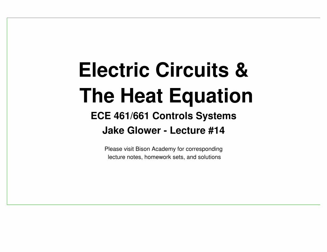
Circuits & Differential Equations

Each energy storage elements adds one differential equation

Inductors: Energy = 1

2LI2

Capacitors: Energy = 1

2CV2

Energy States are

I Inductor

V Capacitor

The differential equations from from

V = LdI

dt

I = CdV

dt

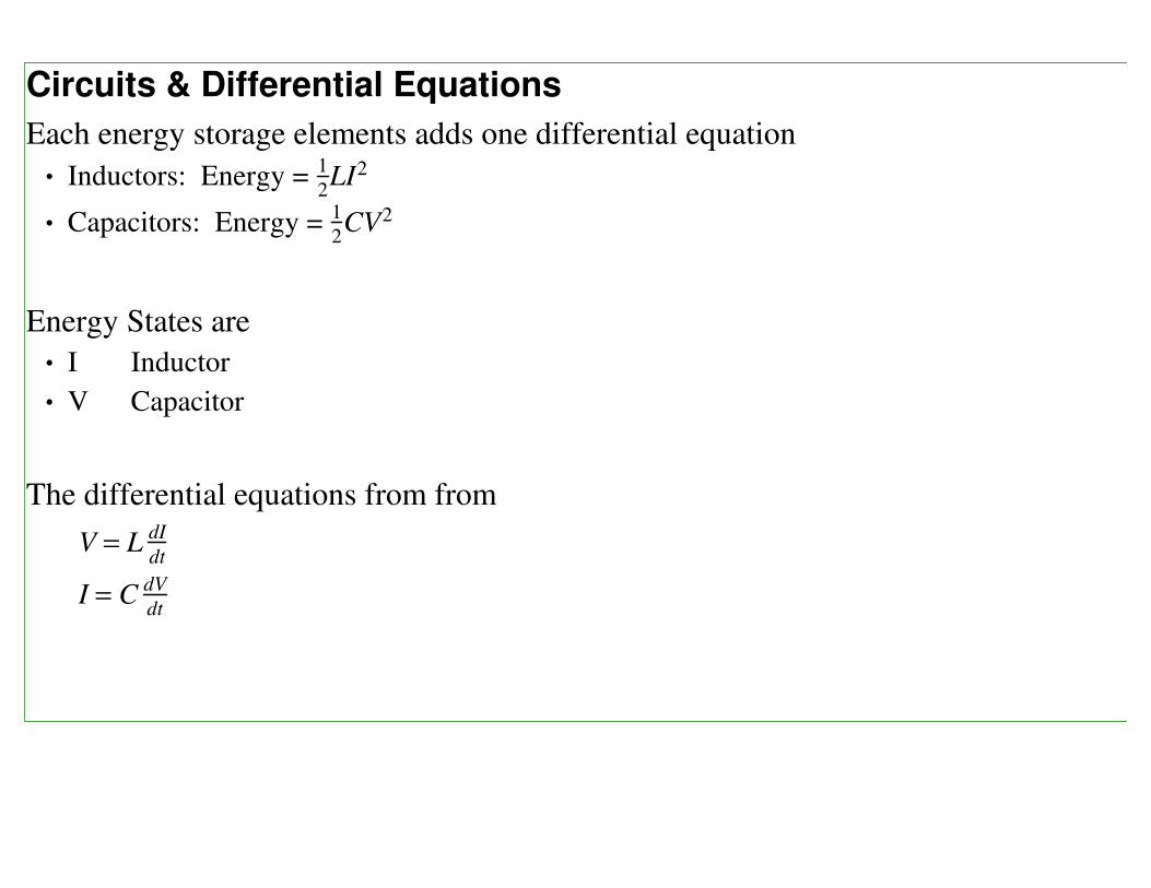
Example #1: RLC Circuit

Dynamics

V1 = LsI1 = V0 − V2

I2 = CsV2 = I1 − I3 −V2

R

V3 = LsI3 = V2 − V4

I4 = CsV4 = I3 −V4

R

State Space

s

I1

V2

I3

V4

=

0

−1

L 0 0

1

C

−1

RC

−1

C 0

0

1

L 0

−1

L

0 0

1

C

−1

RC

I1

V2

I3

V4

+

1

L

0

0

0

V0

+

-V0

I1 I2 I3 I4

V2 V4 = Y+ V1 - + V3 -

L L

C C

RR

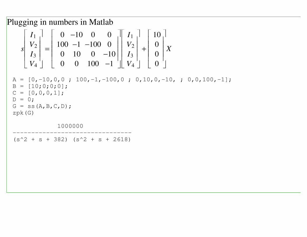
Plugging in numbers in Matlab

s

I1

V2

I3

V4

=

0 −10 0 0

100 −1 −100 0

0 10 0 −10

0 0 100 −1

I1

V2

I3

V4

+

10

0

0

0

X

A = [0,-10,0,0 ; 100,-1,-100,0 ; 0,10,0,-10, ; 0,0,100,-1];

B = [10;0;0;0];

C = [0,0,0,1];

D = 0;

G = ss(A,B,C,D);

zpk(G)

1000000

--------------------------------

(s^2 + s + 382) (s^2 + s + 2618)

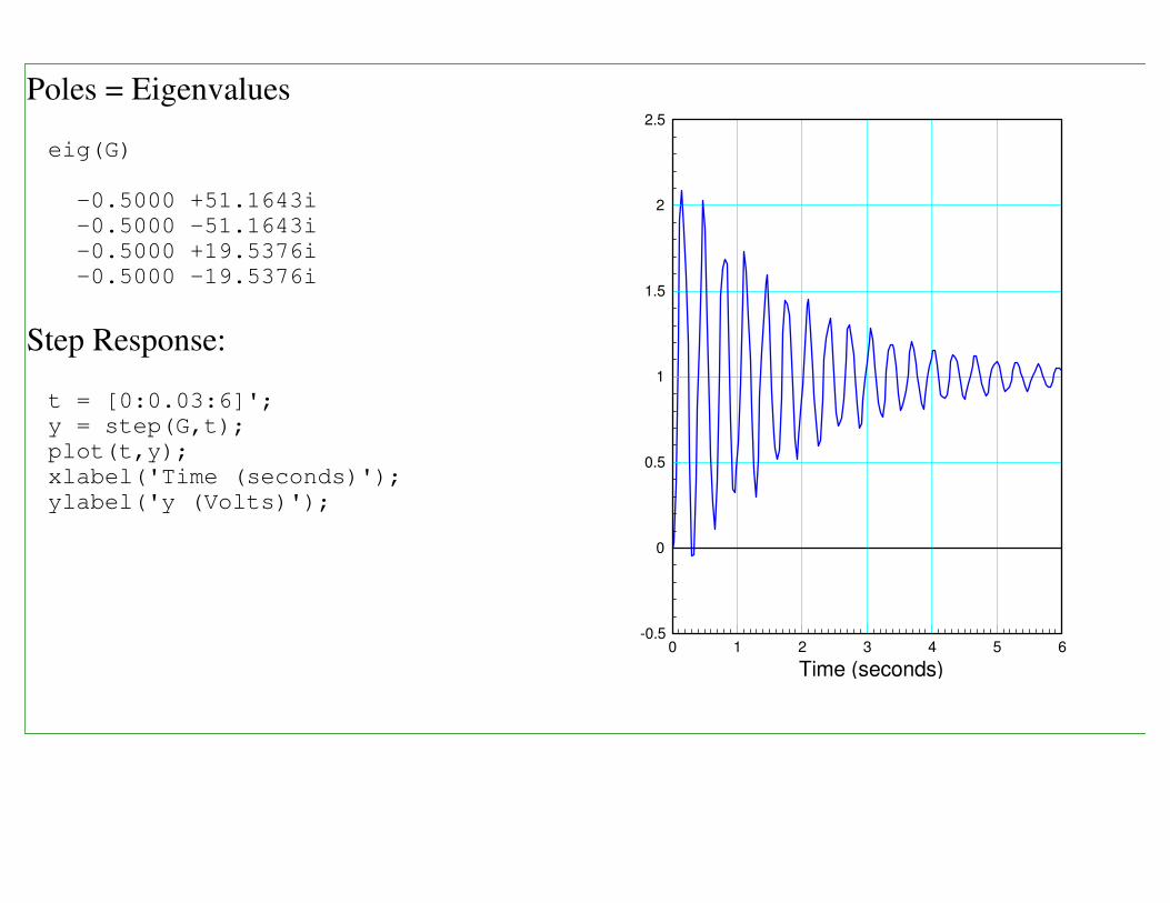
Poles = Eigenvalues

eig(G)

-0.5000 +51.1643i

-0.5000 -51.1643i

-0.5000 +19.5376i

-0.5000 -19.5376i

Step Response:

t = [0:0.03:6]';

y = step(G,t);

plot(t,y);

xlabel('Time (seconds)');

ylabel('y (Volts)');

0 1 2 3 4 5 6-0.5

0

0.5

1

1.5

2

2.5

Time (seconds)

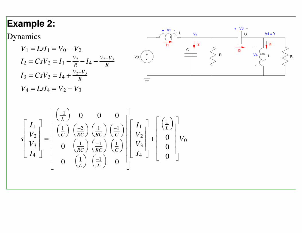
Example 2:

Dynamics

V1 = LsI1 = V0 − V2

I2 = CsV2 = I1 −V2

R− I4 −

V2−V3

R

I3 = CsV3 = I4 +V2−V3

R

V4 = LsI4 = V2 − V3

s

I1

V2

V3

I4

=

−1

L 0 0 0

1

C

−2

RC

1

RC

−1

C

0

1

RC

−1

RC

1

C

0

1

L

−1

L 0

I1

V2

V3

I4

+

1

L

0

0

0

V0

+

-V0

I1 I2

I3

I4

V2 V4 = Y+ V1 -

+ V3 -

L

L

C

RR

+

V4

-

C

Substituting L = 100mH, C = 10mF, R = 50

I1

V2

V3

I4

=

−10 0 0 0

100 −4 2 −100

0 2 −2 100

0 10 −10 0

I1

V2

V3

I4

+

10

0

0

0

Vin

Y = V2 − V3

Throwing it in MATLAB:

A = [-10,0,0,0;100,-4,2,-100;0,2,-2,100;0,10,-10,0];

B = [10;0;0;0];

C = [0,1,-1,0];

D = 0;

G = ss(A,B,C,D);

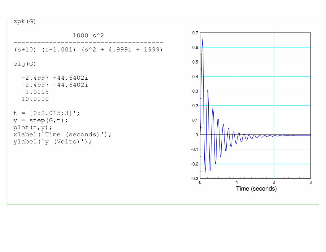
zpk(G)

1000 s^2

--------------------------------------

(s+10) (s+1.001) (s^2 + 4.999s + 1999)

eig(G)

-2.4997 +44.6402i

-2.4997 -44.6402i

-1.0005

-10.0000

t = [0:0.015:3]';

y = step(G,t);

plot(t,y);

xlabel('Time (seconds)');

ylabel('y (Volts)');

0 1 2 3-0.3

-0.2

-0.1

0

0.1

0.2

0.3

0.4

0.5

0.6

0.7

Time (seconds)

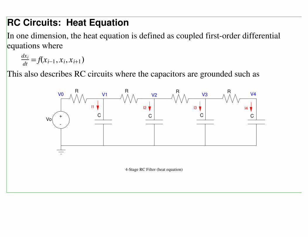
RC Circuits: Heat Equation

In one dimension, the heat equation is defined as coupled first-order differential

equations wheredxi

dt= f(xi−1, xi, x i+1)

This also describes RC circuits where the capacitors are grounded such as

R R R RV1 V2 V3 V4

I1 I2 I3 I4

+

-

V0

VoC C C C

4-Stage RC Filter (heat equation)

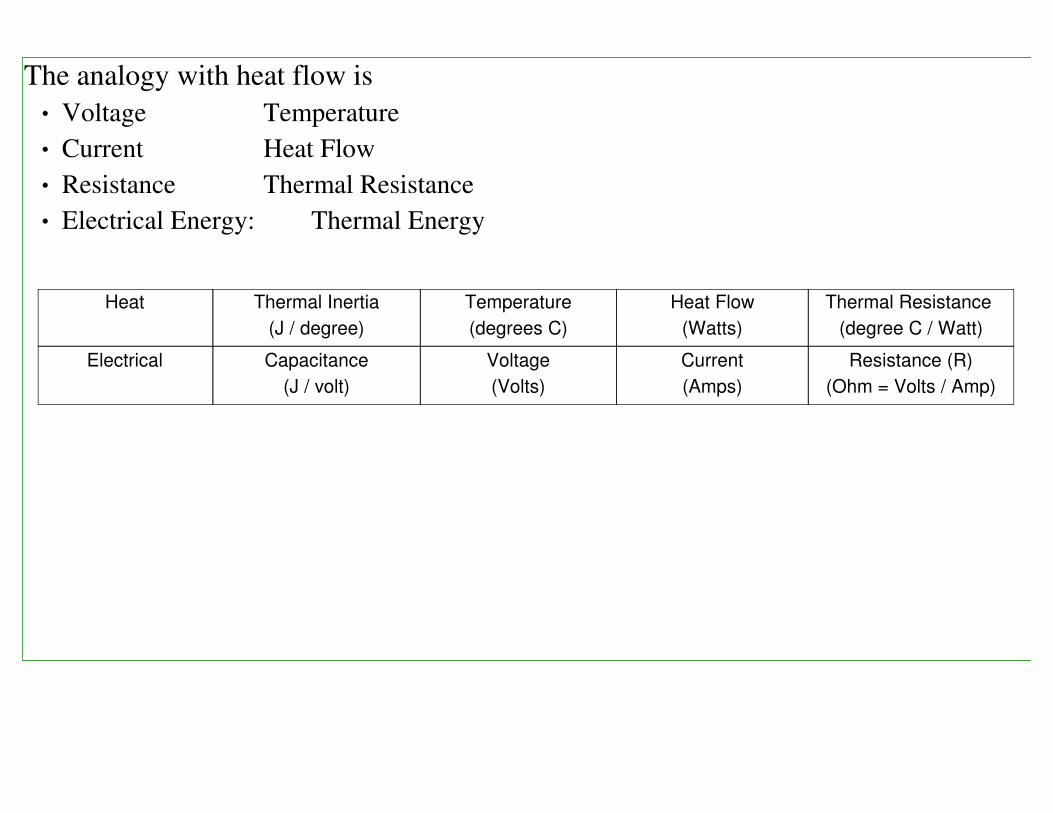
The analogy with heat flow is

Voltage Temperature

Current Heat Flow

Resistance Thermal Resistance

Electrical Energy: Thermal Energy

Heat Thermal Inertia

(J / degree)

Temperature

(degrees C)

Heat Flow

(Watts)

Thermal Resistance

(degree C / Watt)

Electrical Capacitance

(J / volt)

Voltage

(Volts)

Current

(Amps)

Resistance (R)

(Ohm = Volts / Amp)

I1 = CsV1 =

V0−V1

R +

V2−V1

R

I2 = CsV2 =

V1−V2

R +

V3−V2

R

I3 = CsV3 =

V2−V3

R +

V4−V3

R

I4 = CsV4 =

V3−V4

R

sV1

sV2

sV3

sV4

=

−2

RC

1

RC 0 0

1

RC

−2

RC

1

RC 0

0

1

RC

−2

RC

1

RC

0 0

1

RC

−1

RC

V1

V2

V3

V4

+

1

RC

0

0

0

V0

R R R RV1 V2 V3 V4

I1 I2 I3 I4

+

-

V0

VoC C C C

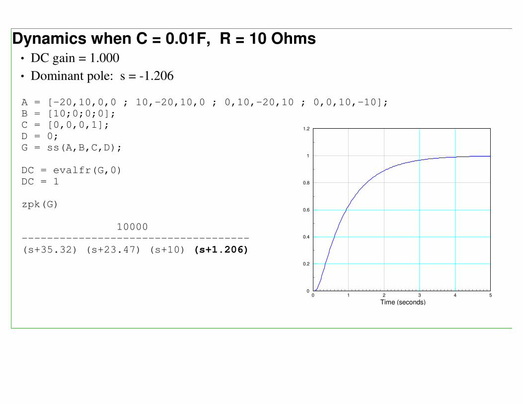
Dynamics when C = 0.01F, R = 10 OhmsDC gain = 1.000

Dominant pole: s = -1.206

A = [-20,10,0,0 ; 10,-20,10,0 ; 0,10,-20,10 ; 0,0,10,-10];

B = [10;0;0;0];

C = [0,0,0,1];

D = 0;

G = ss(A,B,C,D);

DC = evalfr(G,0)

DC = 1

zpk(G)

10000

------------------------------------

(s+35.32) (s+23.47) (s+10) (s+1.206)

0 1 2 3 4 50

0.2

0.4

0.6

0.8

1

1.2

Time (seconds)

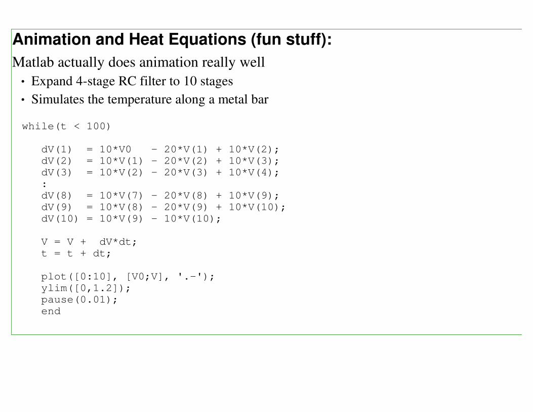
Animation and Heat Equations (fun stuff):

Matlab actually does animation really well

Expand 4-stage RC filter to 10 stages

Simulates the temperature along a metal bar

while(t < 100)

dV(1) = 10*V0 - 20*V(1) + 10*V(2);

dV(2) = 10*V(1) - 20*V(2) + 10*V(3);

dV(3) = 10*V(2) - 20*V(3) + 10*V(4);

:

dV(8) = 10*V(7) - 20*V(8) + 10*V(9);

dV(9) = 10*V(8) - 20*V(9) + 10*V(10);

dV(10) = 10*V(9) - 10*V(10);

V = V + dV*dt;

t = t + dt;

plot([0:10], [V0;V], '.-');

ylim([0,1.2]);

pause(0.01);

end

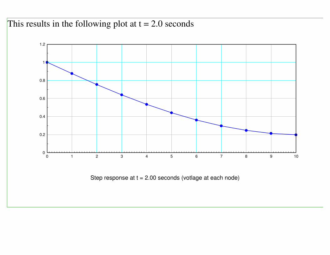
This results in the following plot at t = 2.0 seconds

0 1 2 3 4 5 6 7 8 9 100

0.2

0.4

0.6

0.8

1

1.2

Step response at t = 2.00 seconds (votlage at each node)

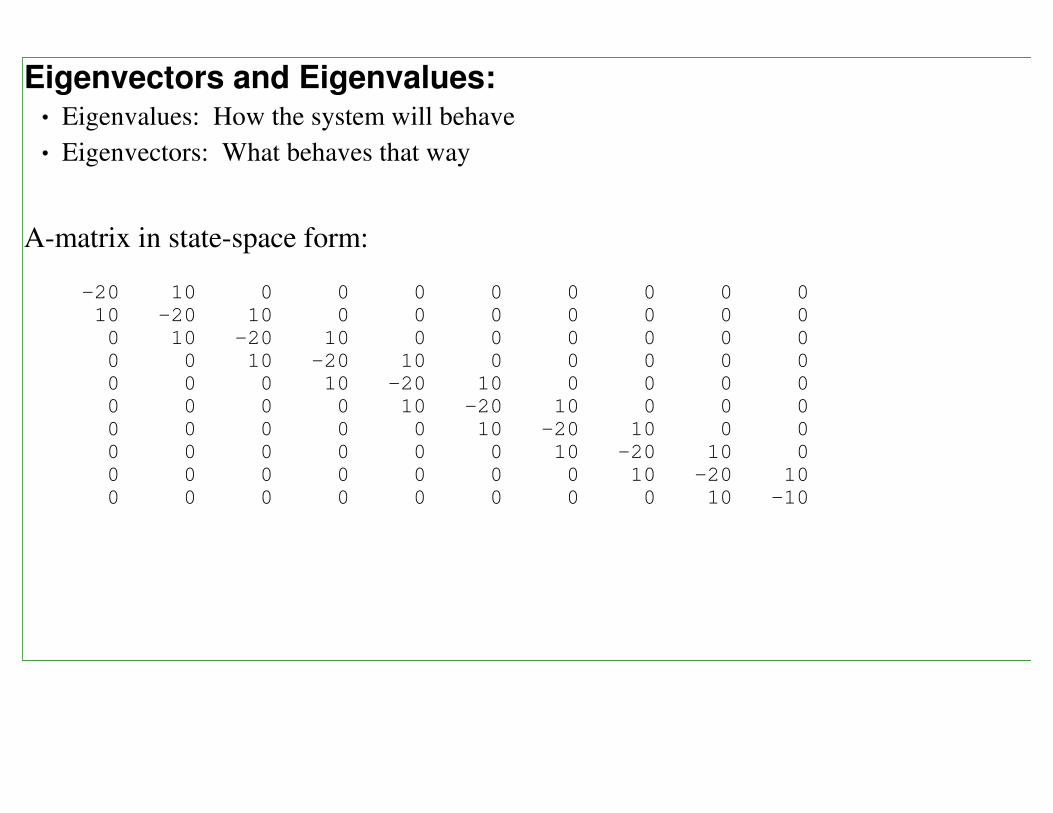
Eigenvectors and Eigenvalues:Eigenvalues: How the system will behave

Eigenvectors: What behaves that way

A-matrix in state-space form:

-20 10 0 0 0 0 0 0 0 0

10 -20 10 0 0 0 0 0 0 0

0 10 -20 10 0 0 0 0 0 0

0 0 10 -20 10 0 0 0 0 0

0 0 0 10 -20 10 0 0 0 0

0 0 0 0 10 -20 10 0 0 0

0 0 0 0 0 10 -20 10 0 0

0 0 0 0 0 0 10 -20 10 0

0 0 0 0 0 0 0 10 -20 10

0 0 0 0 0 0 0 0 10 -10

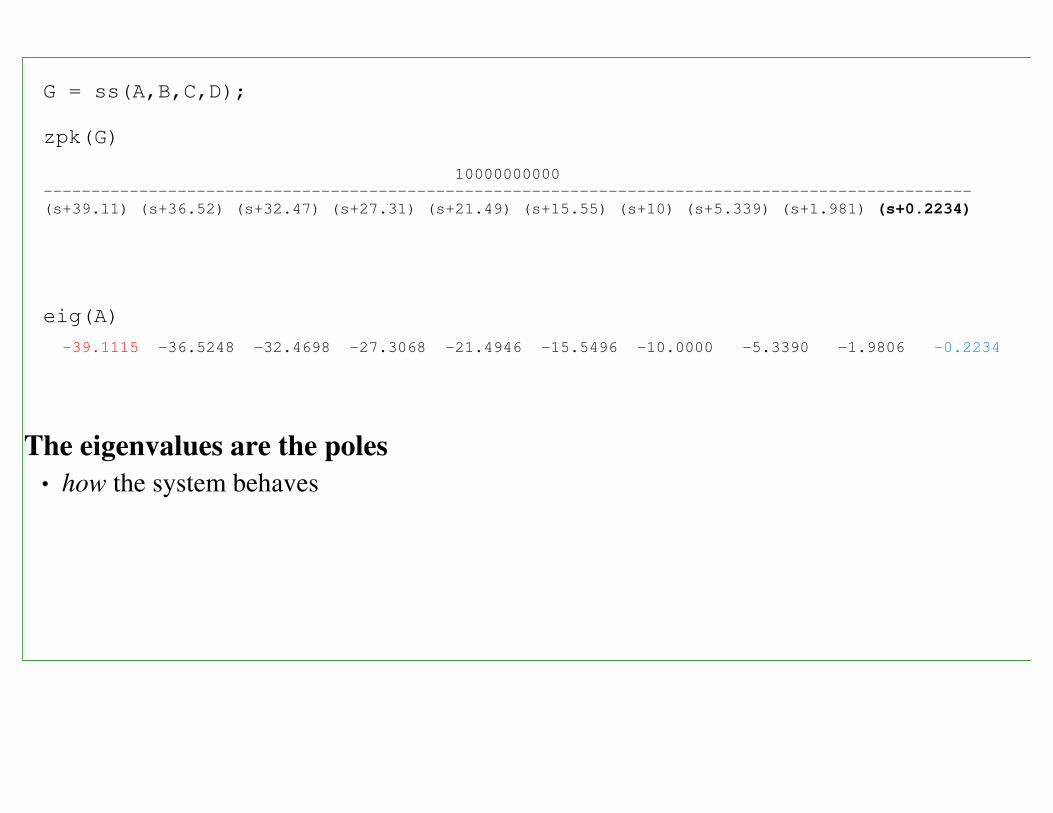
G = ss(A,B,C,D);

zpk(G)

10000000000

-------------------------------------------------------------------------------------------------

(s+39.11) (s+36.52) (s+32.47) (s+27.31) (s+21.49) (s+15.55) (s+10) (s+5.339) (s+1.981) (s+0.2234)

eig(A)

-39.1115 -36.5248 -32.4698 -27.3068 -21.4946 -15.5496 -10.0000 -5.3390 -1.9806 -0.2234

The eigenvalues are the poles

how the system behaves

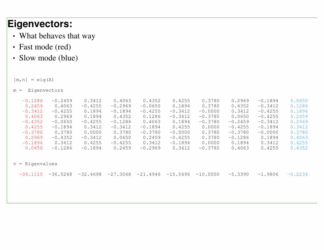
Eigenvectors:What behaves that way

Fast mode (red)

Slow mode (blue)

[m,n] = eig(A)

m = Eigenvectors

-0.1286 -0.2459 0.3412 0.4063 0.4352 0.4255 0.3780 0.2969 -0.1894 0.0650

0.2459 0.4063 -0.4255 -0.2969 -0.0650 0.1894 0.3780 0.4352 -0.3412 0.1286

-0.3412 -0.4255 0.1894 -0.1894 -0.4255 -0.3412 -0.0000 0.3412 -0.4255 0.1894

0.4063 0.2969 0.1894 0.4352 0.1286 -0.3412 -0.3780 0.0650 -0.4255 0.2459

-0.4352 -0.0650 -0.4255 -0.1286 0.4063 0.1894 -0.3780 -0.2459 -0.3412 0.2969

0.4255 -0.1894 0.3412 -0.3412 -0.1894 0.4255 0.0000 -0.4255 -0.1894 0.3412

-0.3780 0.3780 0.0000 0.3780 -0.3780 -0.0000 0.3780 -0.3780 -0.0000 0.3780

0.2969 -0.4352 -0.3412 0.0650 0.2459 -0.4255 0.3780 -0.1286 0.1894 0.4063

-0.1894 0.3412 0.4255 -0.4255 0.3412 -0.1894 0.0000 0.1894 0.3412 0.4255

0.0650 -0.1286 -0.1894 0.2459 -0.2969 0.3412 -0.3780 0.4063 0.4255 0.4352

v = Eigenvalues

-39.1115 -36.5248 -32.4698 -27.3068 -21.4946 -15.5496 -10.0000 -5.3390 -1.9806 -0.2234

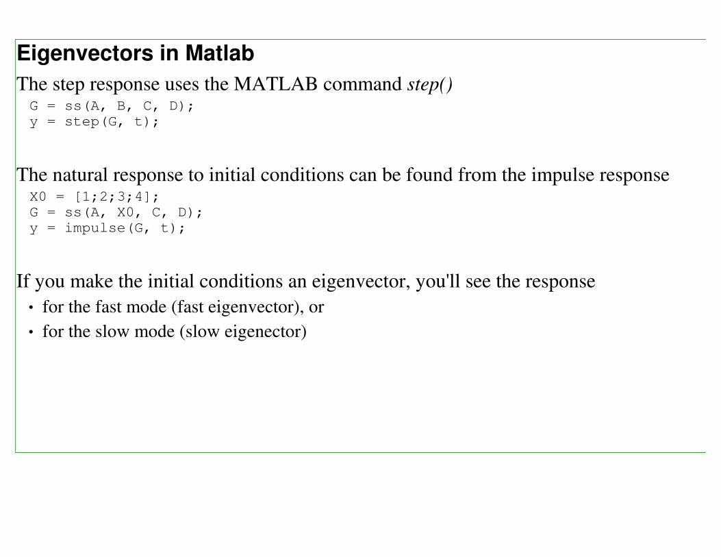
Eigenvectors in Matlab

The step response uses the MATLAB command step()G = ss(A, B, C, D);

y = step(G, t);

The natural response to initial conditions can be found from the impulse responseX0 = [1;2;3;4];

G = ss(A, X0, C, D);

y = impulse(G, t);

If you make the initial conditions an eigenvector, you'll see the response

for the fast mode (fast eigenvector), or

for the slow mode (slow eigenector)

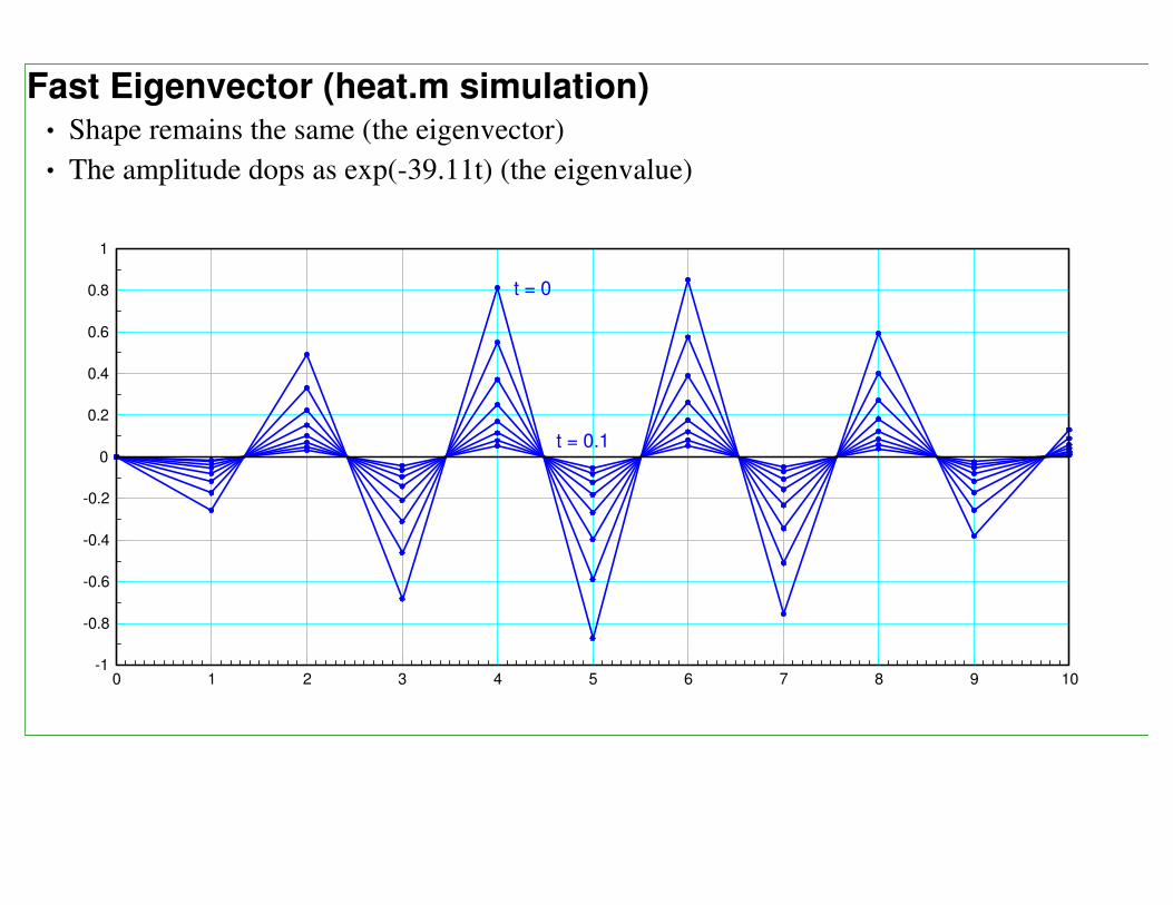
Fast Eigenvector (heat.m simulation)Shape remains the same (the eigenvector)

The amplitude dops as exp(-39.11t) (the eigenvalue)

0 1 2 3 4 5 6 7 8 9 10-1

-0.8

-0.6

-0.4

-0.2

0

0.2

0.4

0.6

0.8

1

t = 0

t = 0.1

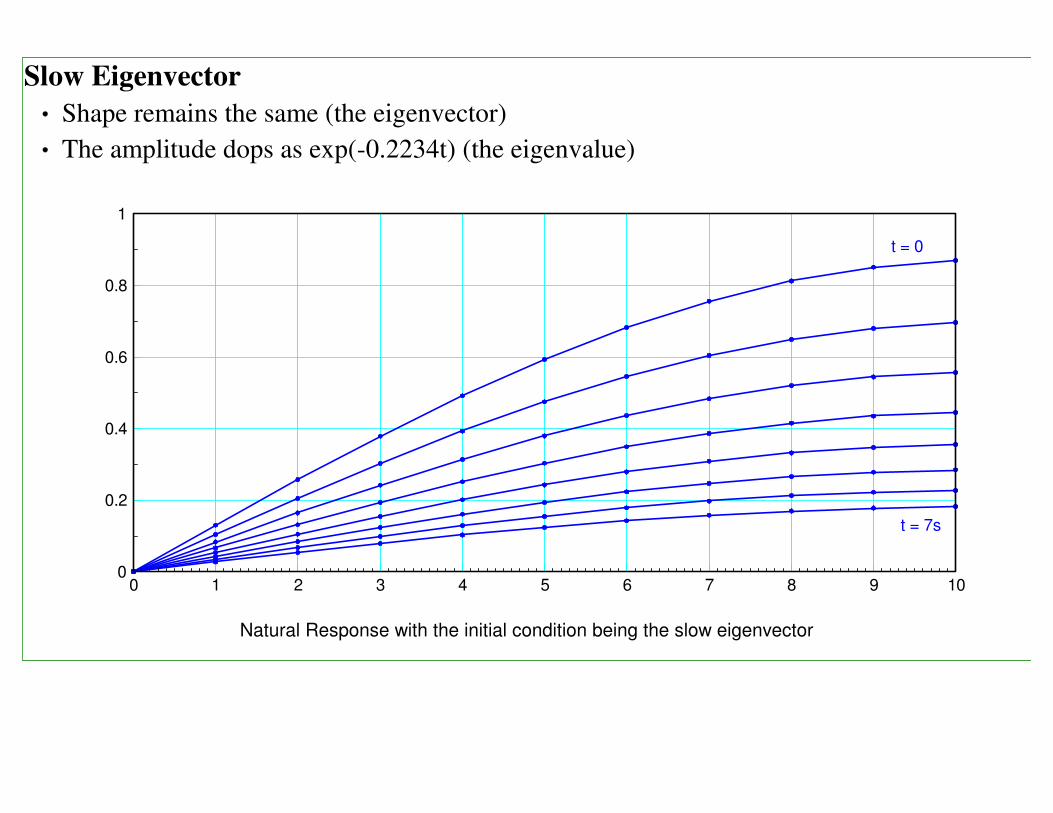
Slow Eigenvector

Shape remains the same (the eigenvector)

The amplitude dops as exp(-0.2234t) (the eigenvalue)

0 1 2 3 4 5 6 7 8 9 100

0.2

0.4

0.6

0.8

1

t = 0

t = 7s

Natural Response with the initial condition being the slow eigenvector

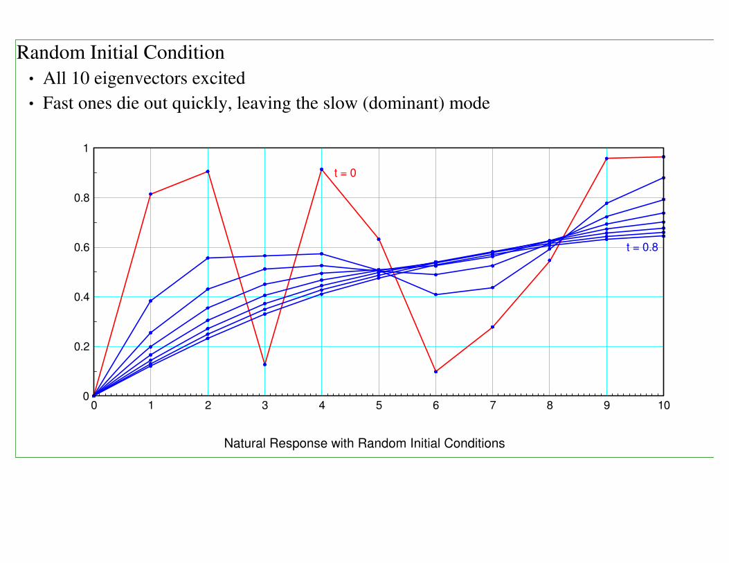
Random Initial Condition

All 10 eigenvectors excited

Fast ones die out quickly, leaving the slow (dominant) mode

0 1 2 3 4 5 6 7 8 9 100

0.2

0.4

0.6

0.8

1

t = 0

t = 0.8

Natural Response with Random Initial Conditions