Th - Energiteknologi · Project title Active filter functionalities for power converters in wind power plants Project identification (pro-gram abbrev. and file) 12188 Name of the

1

Version: november 2014

1.1. Project details

Project title Active filter functionalities for power converters in

wind power plants

Project identification (pro-

gram abbrev. and file)

12188

Name of the programme

which has funded the project

FORSKEL

Project managing com-

pany/institution (name and ad-

dress)

Aalborg University

Project partners

Aalborg University, Dong Energy Wind Power, ABB AB,

Vestas Wind Systems A/S

CVR (central business reg-

ister)

29 10 23 84

Date for submission

1.2. Short description of project objective and results

The purpose of the project is to analyse and develop advanced Active Filter (AF) solutions

based on implementation at the STATCOM level present in the WPP. Emphasis is given to make

the AF efficient and stable during the continuously changing scenario of the network harmonic

composition and WPP transients. Initially the possibility to consider hybrid AF was examined

but it was agreed to drop the passive filtering part for economic reasons. Also, it was agreed

to drop the AF at WT level as the focus is on AF at PCC.

The expected results are in the form of new AF control strategies possible to implement at

the STATCOM level. The methods are developed and tested with in simulation considering

Anholt WPP as a test-bench with the addition of the STATCOM at a 220 kV terminal in the WPP

and voltage harmonics control at the 400 kV terminal in the grid according to specified har-

monic limits. The strategies have to be validated experimentally using RTDS environment.

1.3. Executive summary

The project succeeded in solving the following main challenges:

FDNE grid models in PSCAD and RSCAD to replicate realistic grid impedance scan

data.

Analysis and implementation of harmonic compensation by emulation of resistive behaviour at the selected harmonic frequencies.

2


Development of novel voltage and current feedback AF strategy to be implemented

in a remote connected STATCOM able to attenuate the harmonics amplification due to WPP or reduce the harmonics level to a lower limit without the need of grid impedance knowledge.

The methods have been compared in terms of:

o Total compensation current (RMS) for same attenuation to the background level

o Ability to reduce the harmonics at T1 to lower levels and effect on down-stream busbars (T3, T4 and T5)

o Efficient compensation and stable operation for

The stability of the methods has been verified by RTDS and it was demonstrated

for 16 different cases of grid impedance profile (the remaining 8 cases were not successfully represented as FDNE and we could not simulate them)

The following challenges remain still unsolved and could be considered as future work:

Complete stability analysis theory (the difficulty is that the grid impedance is a very non-linear system with variable parameters)

Improved FDNE modelling

The obtained results can be used by partners as new AF strategies to be implemented in real plants.

1.4. Project objectives

Test benchmark model of the WPP

Active filtering strategies STATCOM in WPP

Implementation of active filtering at STATCOM level

Demonstration on RTDS

1.5. Project results and dissemination of results

1.1.1 Plant description

Anholt offshore wind power plant (Fig. 1) is used here as the reference for developing the

benchmark WPP model. The key details are:

400 MW offshore wind power plant comprising of 111 SWT-3.6-120 WTGs.

Connected to the 400 kV grid at the onshore substation at Trige via two units of

400/220 kV, 450 MVA auto-transformers.

58 km aluminum 3x1x2000 mm2 , 220 kV underground cable

24.5 km 3x1600 mm2 220 kV sub-marine cable.

4x60 MVAr reactors at 220kV onshore transformer terminals

2x60 MVAr reactors at the 220 kV terminal between the onshore and offshore cable

sections.

3x140 MVA, 220/33 kV plant step-up transformers.

The collector grid has a total cable length of 152 km at 33 kV. The equivalent cable

capacitance is 42 uF.

3


AC

40

0kV

22

0kV

33

kV

3x1x2000 mm2

58 km, ug cable

2 x 450 MVAAuto-trafo

3x1600 mm2 24.5 km sm cable

240 MVArReactor

120 MVArReactor

3 x 140 MVATrafo

T1

T2

T3

T4

T5C

T5A

T5BAPF @ T2APF @ T1

Fig. 1. WPP electrical network model.

The partners provided 24 sets of grid impedance vs frequency characteristics. These were modelled using the fre-quency dependent network equivalent (FDNE) components.

1.1.1.1 Background voltage harmonics in the grid model

The grid is represented by a Thevenin’s equivalent voltage source with a frequency de-

pendent series impedance. In DigSILENT, the background harmonic data can be entered in the

form of a data table. In PSCAD and RSCAD, these have to be put in FORTRAN and C-Files

respectively. The phase angles of the individual harmonic component and phase is assigned

such that the different harmonic orders appear as positive, negative or zero sequence compo-

nents.

Fig. 2. Different target harmonic level: Background (Blue), recommended (Yellow) and

planned (Green)

4


Fig. 3. Vector fitting of the impedance data. The continuous curve represents the input data,

and the discrete stems indicate the impedance values at different harmonic orders.

1.1.1.2 Frequency dependent network equivalent (FDNE) for the grid impedance

In DigSILENT, the grid impedance data can be entered as a table of impedance values

against frequency. However, in PSCAD and RSCAD, the impedance vs. frequency characteris-

tics has to be converted into a transfer function using the curve-fitting algorithm developed by

SINTEF[**]. It gives the A, B, C and D parameters of the frequency dependent admittance

characteristics which can be simulated in PSCAD and RSCAD using FORTRAN or C –scripts.

Recently PSCAD has introduced library component models to simulate these A, B, C, D model

of the frequency dependent admittance, and this component has been used in this project.

RSCAD has introduced a module which provides the curve fitting and generates the FDNE

component. Fig. 3 gives the results of vector fitting of the grid admittance data. The grid

admittance data in the range from 10 Hz to 1504.5 Hz was fitted with a 24th order transfer

function which gave the fitting error of 0.67%. In RSCAD vector fitting program, all the data

points (from 10 to 3000 Hz) was used.

1.1.2 WPP modelling

1.1.2.1 WTG

Type 4 wind turbines are considered in this project. Therefore, only the grid side converter

has been modelled in terms of the average model. The dc link capacitor of 72mF has been

modelled, which corresponds to a time constant of 11 ms at 1.05 kV dc link voltage reference.

The model is shown in Fig. 4.

5


(a) Average model of the wind turbine grid side converter

(c) Current control of the grid side converter

(b) DC link capacitor model.

Fig. 4 Wind turbine model

1.1.2.2 WPP collection system and Transients in the collection system

As shown in Fig. 5. WPP model for transient simulation in PSCAD., the WPP collector

system comprises three 140-MVA, 225/32 kV plant step-up transformers which connects the

three collector feeders to the 220-kV bus T4. Each of the 33-kV feeder has 37x3.6 MW WT

connected to it. In this simulation, the WTs on each feeder are grouped into three units of

6


10x3.6-MW and a 7x3.6-MW unit. The power order to these units are given from the control

panel by the sliders, P10 and P7 respectively. The control panel also controls the circuit break-

ers in each feeders. The circuit breakers are included in this simulation so that the individual

feeders can be connected7disconnected to create the transients in the WPP network.

T3

T4

10 WT units

7 WT units

Control Panel: P10, P7 order and CB control

Fig. 5. WPP model for transient simulation in PSCAD.

1.1.2.3 Export cables

1.1.2.3.1 Underground Cable

The 58 km underground cable is laid in flat formation. Hence initially it was modelled in

flat formation as shown in, using cable data from Error! Reference source not found.. A

single layover section has been modelled as shown in Error! Reference source not

found.(a). The relevant conductivity and relative permittivity data of the core, sheath and

insulating layers are as follows: 𝜌𝑐 = 3.547 × 10−8Ωm, 𝜌𝑠 = 2.676 × 10−8Ωm, 𝜖𝑖1 = 2.89, 𝜖𝑖2 = 2.3.

The cables are buried at a depth of 1.3 m with a separation of 0.4 m between them.

7


(a) Underground cable layout model.

(b) Flat layout of 3x1 2000 sq. mm underground cable

Fig. 6. Underground cable model.

Such a cable has unbalanced mutual coupling between the phases A and B, and A and C.

Such an unbalance creates coupling between the sequence impedances. Hence it was decided

to use trefoil layout of the cables in the PSCAD simulation and RSCAD implementation.

Fig. 7. Comparison of underground cable (in trefoil and in flat formation) impedance charac-

teristics in DigSILENT and PSCAD.

8


1.1.2.3.2 Submarine Cable

The 24.5 km submarine cable is modelled as three conductor cores in trefoil formation.

Only two conducting layers, viz. the core and the inner sheath have been included in the model

so as to maintain the similarity of the models in DigSILENT and PSCAD models.

1.1.3 Harmonics compensation strategies

This section describes theoretical solutions identified on the basis of mathematical analysis

and validated by PLECS simulation for harmonic compensation for the wind power plant (WPP)

model. We use a simplified three-impedance model of the grid and WPP and study the harmonic

compensation effectiveness at bus T1, when the STATCOM with active power filter (APF) is

connected at bus T2. In all subsequent figures Z1 is the equivalent grid impedance, Z2 is the

equivalent wind far m impedance, ZT is the super-transformer impedance, and ZAPF is the vir-

tual impedance created by the active power filter. The voltages at busses T1 and T2 are de-

noted by V1 and V2, and Vh is the harmonic source in the grid.

1.1.3.1 Compensation at T2 with voltage feedback from T1

This section describes a harmonic voltage controller based on the voltage feedback from

bus T1. The WPP model in Fig. 8 shows the APF as a controlled current source that produces

the current IF as a function of the T1 voltage. Voltages V1 and V2 at busses T1 and T2, are

given by (1).

𝑉1 = 𝑉ℎ𝑍2+𝑍𝑇

𝑍1+𝑍2+𝑍𝑇−

𝑍1𝑍2

𝑍1+𝑍2+𝑍𝑇𝐼𝐹 𝑉2 = 𝑉ℎ

𝑍2

𝑍1+𝑍2+𝑍𝑇−

(𝑍1+𝑍𝑇)𝑍2

𝑍1+𝑍2+𝑍𝑇𝐼𝐹 (1)

In the most general case the APF current is controlled by the T1 voltage by means of a

virtual impedance ZAPF, as 𝐼𝐹 = 𝐾𝑉1/𝑍𝐴𝑃𝐹. Assuming the virtual impedance equal to Z2, 𝑍𝐴𝑃𝐹 = 𝑍2,

the voltage at bus T1 is (2) and the filter current is 𝐼𝐹 = 𝐾𝑉1/𝑍2.

𝑉1 = 𝑉ℎ𝑍2+𝑍𝑇

(1+𝐾)𝑍1+(𝑍2+𝑍𝑇) or, 𝐴1 =

𝑉1

𝑉ℎ=

𝑍2+𝑍𝑇

(1+𝐾)𝑍1+(𝑍2+𝑍𝑇) (2)

The static characteristic of the amplification ratio A1 in (2) is shown in Fig. 9. It clearly

shows, that the amplification ratio is unity for 𝑘 = −1.

Fig. 8. Simplified wind farm model with compensation at T2 based on T1 voltage feedback.

9


Fig. 9. Amplification at T1 due to the harmonic compensation at T2 using 𝐼𝑓 =𝑘𝑉1

𝑍2

The goal is to keep the voltage magnitude at T1 equal to the grid voltage magnitude, i.e.

|𝑉1| = |𝑉ℎ|. This condition is satisfied by two values for gain K.

𝐾1 = −1 𝐾2 = −𝑅1

2+𝑋12+2𝑅1𝑅2+2𝑅1𝑅𝑇+2𝑋1𝑋2+2𝑋1𝑋𝑇

𝑅12+𝑋1

2 (3)

Solution K1 is constant and always exists, while solution K2 depends on all impedances and

it is impractical for implementation as a controller with constant gain. However, it can be

implemented by a closed loop feedback controller. Solution K2 is positive for all cases when

grid harmonics are amplified at T1 (h = 11, 13, 17, 19) and it is negative for other harmonic

orders (h = 5, 7). Voltage V1 can be reduced to any small value if K is large enough.

Similar solutions have been found for resistive feedback, 𝑍𝐴𝑃𝐹 = 𝑅2, and inductive feedback,

𝑍𝐴𝑃𝐹 = 𝑋2. In these cases all solutions depend on all impedance present in the system. The

most advantageous for implementation is the gain 𝐾1 = −1, which works for the complex virtual

impedance case.

1.1.3.1.1 Dynamic analysis and Controller Design

For our case study, the grid and the WPP impedances are capacitive for harmonic orders k

= 5 and 7. The voltage controller transfer function that implements the complex feedback, 𝐼𝐹 =

𝐾𝑉1/𝑍2 is (4)

𝐻𝐴𝑃𝐹 =𝐼𝐹

∗

𝑉1= 𝐾

𝐶2𝑠

𝑅2𝐶2𝑠+1

(4)

For harmonic orders k = 11 and above the WPP impedance is inductive, and the controller

transfer function is (5).


∗

𝑉1= 𝐾

1

𝐿2𝑠+𝑅2 (5)

The sign of gain K is of major importance for the controller stability: a positive gain creates

a negative feedback loop, while a negative gain creates a positive feedback. Although the

positive feedback can be stable under some circumstances (when the loop gain is less than

unity), the negative feedback is always preferred. Thus, the simple solution K1 = –1 in (6)

10


involves positive feedback and the stability of this solution must be carefully verified at imple-

mentation.

The reactive compensation, 𝑍𝐴𝑃𝐹 = 𝑋2, works with low filter currents at positive gains (neg-

ative feedback) and it is advantageous for implementation. The voltage controller that realizes

𝐼𝐹 = 𝐾𝑉1/𝑋2 is a pure derivative transfer function as in (6), for harmonics k = 5 and 7. For a

causal implementation this is combined with a low pass filter with a small time constant T.


∗

𝑉1= 𝐾𝐶2𝑠 ≅ 𝐾

𝐶2𝑠

𝑇𝑠+1 (6)

For harmonic orders k = 11 and above we use either a pure integrator, or a low pass filter

(LPF) with a large time constant, T, as in (7). The LPF solution is practical for implementation.

𝐻𝐴𝑃𝐹 = 𝐾1

𝐿2𝑠≅ 𝐾

1

𝑇𝑠+1 (7)

The resistive compensation, 𝐼𝐹 = 𝐾𝑉1/𝑅2, can be realized with a real proportional gain.

In order to reduce the harmonics at values lower than the background levels the gain K

has been adjusted using an integral controller with slow dynamic response (large time con-

stant). Fig. 10 shows the block diagram of the complete controller used to reduce the harmonic

voltage magnitude to a set value denoted by V1*. The block diagram shows the main controller

HAPF, and the harmonic filter implemented in dq reference frame. This scheme has been im-

plemented for each harmonic order.

Fig. 10. Control block diagram for harmonic compensation at T2 based on T1 voltage feed-

back.

Complex compensation is stable for any positive gain K. Resistive compensation is unstable

for harmonics k = 17 and 19 and approaches the instability limit for harmonics k = 11 and 13.

Reactive compensation is stable for any positive gain K. The controller recommended for im-

plementation is either the complex feedback (4) and (5) or the reactive feedback (6) and (7),

both with positive gains (negative feedback). Apart from the different time constants, the two

controllers are very similar. With negative gains (positive feedback) the system is stable for a

narrow range, 𝐾𝑚𝑖𝑛 < 𝐾 < 0. The gain 𝐾1 = −1, is stable for all harmonic orders and it can be

used for implementation.

This analysis reveals the following aspects that characterize the T1 feedback control:

- The controller with feedback from T1 is able to reduce the harmonics to grid back-

ground levels.

- With large enough feedback gains the controller is able to reduce the harmonics to a

value lower than the grid background levels.

11


- There is always one solution, 𝑍𝐴𝑃𝐹 = −𝑍2, that is independent of the grid impedance

and that is constant as long as Z2 stays constant.

- For reactive feedback the filter currents are lower.

- The filter current is lowest for the resistive feedback. This method is recommended for

implementation.

1.1.3.2 Compensation at T2 with voltage feedback from T2

This section describes the harmonic compensation when the APF is connected at bus T2

and uses the voltage feedback from the same bus. The WPP model in Fig. 11 shows the APF

as a current source that creates a virtual impedance ZAPF. The voltages V1 and V2 at busses T1

and T2, are (8).

𝑉1 = 𝑉ℎ𝑍2𝑍𝐴𝑃𝐹+𝑍𝑇𝑍2+𝑍𝑇𝑍𝐴𝑃𝐹

𝑍1𝑍2+𝑍1𝑍𝐴𝑃𝐹+𝑍2𝑍𝐴𝑃𝐹+𝑍𝑇𝑍2+𝑍𝑇𝑍𝐴𝑃𝐹 𝑉2 = 𝑉ℎ

𝑍2𝑍𝐴𝑃𝐹

𝑍1𝑍2+𝑍1𝑍𝐴𝑃𝐹+𝑍2𝑍𝐴𝑃𝐹+𝑍𝑇𝑍2+𝑍𝑇𝑍𝐴𝑃𝐹 (8)

The APF current is controlled by the T2 voltage by means of a virtual impedance ZAPF, as

𝐼𝐹 = 𝐾𝑉2/𝑍𝐴𝑃𝐹. Assuming the virtual impedance equal to Z2, 𝑍𝐴𝑃𝐹 = 𝑍2, the voltage at bus T1 is

𝑉1 = 𝑉ℎ𝑍2𝑍𝑇(𝐾+1)+𝑍2

2

𝑍1𝑍2(𝐾+1)+𝑍2𝑍𝑇(𝐾+1)+𝑍22 (9)

The goal is to keep the voltage magnitude at T1 equal to the grid voltage magnitude, i.e.

|𝑉1| = |𝑉ℎ|. This condition is satisfied by two values for gain K.

𝐾1 = −1 𝐾2 = −𝑅1

2+𝑋12+2𝑅1𝑅𝑇+2𝑋1𝑋𝑇+2𝑅1𝑅2+2𝑋1𝑋2

𝑅12+𝑋1

2+2𝑅1𝑅𝑇+2𝑋1𝑋𝑇 (10)

Fig. 11. Simplified model of the wind power farm and active filter for compensation at T2.

Solution K1 is constant and always exists, while solution K2 depends on all impedances and

it is impractical for implementation. To implement this approach with a predetermined constant

gain K, the APF current reference will be set to 𝐼𝐹 = 𝐾𝑉2/𝑍2.

A similar analysis have been carried out for resistive compensation, 𝑍𝐴𝑃𝐹 = 𝑅2, and for re-

active compensation with 𝑍𝐴𝑃𝐹 = 𝑗𝑋2. The solutions are quite similar in both cases. The conclu-

sion is that the resistive and reactive compensation alone are unable to provide compensation

12


under all possible functional situations. Only the complex compensation is able to reduce the

harmonics to background levels.


The voltage controller transfer function that implements the complex feedback, 𝐼𝐹 = 𝐾𝑉2/𝑍2

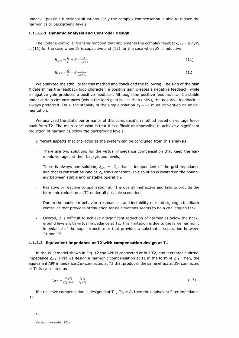
is (11) for the case when Z2 is capacitive and (12) for the case when Z2 is inductive.


∗

𝑉2= 𝐾

𝐶2𝑠

𝑅2𝐶2𝑠+1 (11)


∗

𝑉2= 𝐾

1

𝐿2𝑠+𝑅2 (12)

We analyzed the stability for this method and concluded the following. The sign of the gain

K determines the feedback loop character: a positive gain creates a negative feedback, while

a negative gain produces a positive feedback. Although the positive feedback can be stable

under certain circumstances (when the loop gain is less than unity), the negative feedback is

always preferred. Thus, the stability of the simple solution 𝐾1 = −1 must be verified on imple-

mentation.

We analyzed the static performance of this compensation method based on voltage feed-

back from T2. The main conclusion is that it is difficult or impossible to achieve a significant

reduction of harmonics below the background levels.

Different aspects that characterize the system can be concluded from this analysis:

- There are two solutions for the virtual impedance compensation that keep the har-

monic voltages at their background levels;

- There is always one solution, 𝑍𝐴𝑃𝐹 = −𝑍2, that is independent of the grid impedance

and that is constant as long as Z2 stays constant. This solution is located on the bound-

ary between stable and unstable operation.

- Resistive or reactive compensation at T1 is overall ineffective and fails to provide the

harmonic reduction at T2 under all possible scenarios.

- Due to the nonlinear behavior, resonances, and instability risks, designing a feedback

controller that provides attenuation for all situations seems to be a challenging task.

- Overall, it is difficult to achieve a significant reduction of harmonics below the back-

ground levels with virtual impedance at T2. This limitation is due to the large harmonic

impedance of the super-transformer that provides a substantial separation between

T1 and T2.

1.1.3.3 Equivalent impedance at T2 with compensation design at T1

In the WPP model shown in Fig. 12 the APF is connected at bus T2, and it creates a virtual

impedance ZAPF. First we design a harmonic compensation at T1 in the form of ZT1. Then, the

equivalent APF impedance ZAPF connected at T2 that produces the same effect as ZT1 connected

at T1 is calculated as

𝑍𝐴𝑃𝐹 =𝑍𝑇1𝑍2

2

(𝑍2+𝑍𝑇)2 −𝑍𝑇𝑍2

𝑍2+𝑍𝑇 (13)

If a resistive compensation is designed at T1, ZT1 = R, then the equivalent filter impedance

is:

13


𝑍𝐴𝑃𝐹 =𝑅𝑍2

2

(𝑍2+𝑍𝑇)2−

𝑍𝑇𝑍2

𝑍2+𝑍𝑇 (14)

The virtual impedance ZAPF produces the same effect as ZT1 at T1. Its effect at T2 is differ-

ent from that produced by ZT1 at T2.

Fig. 12. Simplified model of the wind power farm and active filter for equivalent compensation

at T2.

The implementation of complex or resistive compensation described by (13) and (14) is

rather involved. In particular, for capacitive impedance Z2, the transfer functions turn out being

non-causal and cannot be implemented. On the other hand, similar functionality is provided

by the current feedback controller described later. The current controller has a much simpler

topology. For all these reasons, this equivalent controller has not been further investigated

and a solution for implementation has not been developed.

1.1.3.4 Harmonic Compensation at T2 with Grid Current feedback

This section describes the harmonic compensation when grid current feedback is employed.

The WPP model in Fig. 13 shows the APF current IF controlled as a function of the grid current

I1, 𝐼𝐹 = 𝐾𝐼1, where K is the gain of transfer function HAPF for each harmonic frequency. K can

assume any real or complex value. The voltages at buses T1 and T2 are (15).

𝑉1 = 𝑉ℎ(1−𝐾)𝑍2+𝑍𝑇

𝑍1+𝑍𝑇+(1−𝐾)𝑍2 𝑉2 = 𝑉ℎ

(1−𝐾)𝑍2

𝑍1+𝑍𝑇+(1−𝐾)𝑍2 (15)

Fig. 13. Simplified wind farm model with compensation at T2 based on grid current feedback.

14


The goal is to have the voltage magnitude V1 equal to grid voltage magnitude Vh. The

solution of equation |𝑉1| = |𝑉ℎ| is the real gain K1 in (16). For this case the compensation can

be implemented using a simple proportional gain that multiplies the grid current, 𝐼𝐹 = 𝐾1𝐼1.

𝐾1 =𝑅1

2+𝑋12+2𝑅1𝑅2+2𝑅1𝑅𝑇+2𝑋1𝑋2+2𝑋1𝑋𝑇

2𝑅1𝑅2+2𝑋1𝑋2 (16)

By analyzing the static performance of this scheme we found that the compensation with

real gain K (i.e. a proportional feedback controller) is able to reduce the harmonics to the

background levels, but it has difficulties to reduce them to values below the background levels.

The voltage at T1 can be reduced below the background levels, all the way down to zero

by using a dynamic controller. The solution for equation 𝑉1 = 0 is (17). This solution does not

depend on the grid impedance Z1. The voltage at bus T2 can also be reduced to zero with 𝐾 =

1.

𝐾0 =𝑍2+𝑍𝑇

𝑍2 (17)

The compensation with complex feedback can be implemented as in (18).

𝐼𝐹 = 𝐾𝑍2+𝑍𝑇

𝑍2𝐼1 (18)


The controller transfer function that provides proportional (P) feedback is (13).


∗

𝐼1= 𝐾 (19)

The gain K must be negative in order for the control system to work with stable negative

feedback.

The controller transfer function that provides complex feedback can be implemented as a

proportional-integral (PI) controller (20).


∗

𝐼1= 𝐾(𝑅 −

𝜔

𝑠𝑋) (20)

where R and X are the resistance and reactance of the equivalent impedance 𝑍 = (𝑍2 + 𝑍𝑇)/𝑍2.

In order to reduce the harmonics at values lower than the background levels the gain K

has been adjusted using an integral controller with slow dynamic response (large time con-

stant). Fig. 14 shows the block diagram of the complete controller used to reduce the harmonic

voltage magnitude to a set value denoted by V1*. The block diagram shows the main controller

HAPF, and the harmonic filter implemented in dq reference frame. This scheme must be imple-

mented for each harmonic order.

To verified the stability for this simplified model using the root locus of the open-loop

transfer function 𝐻0 = 𝐻1𝐻𝐴𝑃𝐹 for each harmonic order. The P controller has the advantage to

preserve the order of (11) or (12), i.e. the closed loop control system is of second order. This

controller is stable for any negative gain K. The PI controller increases the system order by

adding a zero pole.

15


Fig. 14. Control block diagram for harmonic compensation at T2 based on Grid current feed-

back.

We conclude that both controllers are adequate for implementation. The P controller is

very simple and provides harmonic attenuation to background levels. The PI controller adds a

pole and increases the system complexity, but it is able to reduce the harmonics to any value

below background levels, all the way to zero.

1.1.3.5 Harmonic Compensation at T2 with Wind Farm Current Feedback

Fig 7 shows the simplified WPP model when the filter current is controlled as a function of

the wind farm current I2, using the feedback controller with transfer function HAPF. In this case

the filter current is (21) and the T1 voltage is (22).

𝐼𝐹 = 𝐾𝐼2 = 𝐾𝑉2

𝑍2 (21)

𝑉1 = 𝑉ℎ𝑍2+(1+𝐾)𝑍𝑇

(1+𝐾)(𝑍1+𝑍𝑇)+𝑍2 (22)

This case is the same compensation solution described in Chapter 2, as virtual impedance

at T2. All solutions and all conclusions presented in Chapter 2 remain valid for this case. There

are two solutions for harmonic compensation. The simplest one is 𝐾 = −1, which is marginally

stable, while the second one depends on Z1. This case will not be further discussed.

Fig. 7 Simplified wind farm model with compensation at T2 based on WPP current feed-

back.

This analysis reveals the following aspects that characterize the current feedback control:

16


- We identified two solutions based on grid current feedback which are able to reduce

the voltage harmonics at bus T1.

- The first solution is a simple proportional controller that is able to reduce the harmonics

to grid background levels. The closed-loop system with P control is stable for any neg-

ative gain.

- The second solution is a proportional integral controller that is able to reduce the har-

monics to any value lower than the grid background levels. The closed-loop system

with PI control is stable for any positive gain.

- The compensation based on grid current feedback is simple and easy to implement. In

conclusion, the grid current control is recommended for implementation.

1.1.3.6 Conclusion

We have described five distinct methods for harmonic compensation for the wind power

plant simplified model. All methods work with remote compensation – harmonic reduction at

T1 with current injection at T2.

For each method we provide a steady-state analysis that identifies one or more controller

topologies which are able to reduce the harmonics to the grid background levels or to lower

values. A stability analysis that identifies a range of gains for which the closed-loop control

system is stable is also provided for each method. Table I summarizes the most important

properties of the remote compensation methods proposed here.

Table I Main properties of harmonic compensation methods

T2 voltage feed-

back (§1.5.3.2)

Equivalent im-

pedance at T2

(§1.5.3.3)

T1 voltage feed-

back (§1.5.3.1)

Grid current

feedback

(§1.5.3.4)

Remote compensation at

T1

Yes Yes Yes Yes

Reduces harmonics to

grid background levels

Yes Yes Yes Yes

Reduces harmonics to

zero

No Yes Yes Yes

Theoretical stability Yes n/a Yes Yes

Stable in RSCAD simula-

tion

n/a n/a Yes Yes

Number of sub-methods Real and com-

plex

Complex Real and com-

plex

Real and com-

plex

Control complexity simple complex simple simple

Sensors required voltage voltage voltage current

Sensor bandwidth 1 kHz 1 kHz 1 kHz 1 kHz

Recommended No No Yes Yes

17


It is concluded that the most promising methods are the compensation based on T1 voltage

feedback and compensation based on grid current feedback. Therefore, these schemes have

been selected for PSCAD implementation and validation.

1.1.4 PSCAD simulation results (Resistive, kV1/Z2 for ID24)

The method described in T1 voltage feedback (§1.5.3.1) was implemented in PSCAD for

the two sub-cases:

1. Constant gain such that, the compensating filter current is given by, 𝐼𝑓 = −𝑘𝑉1

𝑍2 .

the harmonic voltage amplification at T1 should be unity as per (2). Thus the har-

monic voltages at T1 should be limited to the background levels.

2. Adaptive gain, where, the compensating filter current is given by, 𝐼𝑓 = −𝑘𝑉1

𝑍2 , and

the gain k is obtained by integrating the measure of excess harmonic voltage above

the specified limiting levels as shown in Fig. 10.

For this purpose, the effective WPP impedance (𝑍2) at a particular harmonic order has been

converted into equivalent R-L or R-C elements and relevant time constant for the transfer

functions as shown in Table II. It considers the collector grid cables and the underground

cables in trefoil formation.

Table II Conversion of the WPP harmonic impedance data to equivalent R, and L or C compo-

nents.

Freq(Hz) R(Ohm) X(Ohm) L(H) C(F) tau(sec)

50 54.15 54.83 1.75E-01 -5.81E-05 -3.14E-03

250 6.11 -50.93 -3.24E-02 1.25E-05 7.64E-05

350 4.94 -28.55 -1.30E-02 1.59E-05 7.87E-05

550 6.44 -10.70 -3.10E-03 2.70E-05 1.74E-04

650 8.27 -3.97 -9.72E-04 6.17E-05 5.10E-04

850 9.25 -0.43 -8.08E-05 4.34E-04 4.01E-03

950 10.01 2.54 4.25E-04 -6.60E-05 -6.60E-04

These impedances are emulated to generate the corresponding harmonic current refer-

ences from the corresponding harmonic sequence voltages as shown in the block diagram in

Fig. 14Error! Reference source not found.. The block diagram also shows the extraction of

the sequence components using the Park’s transformation, first order filters and the inverse

park’s transformation. Finally the extracted voltage is multiplied with the WPP admittance

transfer function to obtain the reference currents for the filter.

1.1.4.1 Compensation with constant gain k=1.

The method has been successfully applied in all the 24 grid impedance cases. In every

case, the harmonic voltages tend to approach the background levels is indicated in the first

row. While the 13th harmonic is amplified in all the cases, the 19th harmonic gets amplified

only in the case ID 24. In some cases, like ID=3, 4, 11, 13 and 14, the 13th harmonic voltage

is amplified from 0.5% in the background to 1.19%, 1.16%, 1.16, 1.14 and 1.18% respec-

tively. These results are summarized in Table III , which shows the base case and compensated

case values of the 5th, 7th, 11th, 13th, 17th and the 19th harmonic components. In all these case,

18


the 13th harmonic voltage in the compensated case is limited within 0.544%. The 5th, 7th, and

11th harmonic cases are well attenuated in all these cases. They are included in this simulation

and the report just for the sake of theoretical justification that the voltages tend to move to

the background levels. These cases do not have practical significance, as the attenuated har-

monic levels are preferable.

Table III Simulation of the 24 cases and the effect of harmonic compensation, 𝐼𝑓 = −𝑉1

𝑍2

Harmonics V5N V7P V11N V13P V17N V19P

Back-

ground

0.50% 0.34% 0.44% 0.49% 0.10% 0.42%

ID=3, Base 0.402% 0.166% 0.156% 1.193% 0.096% 0.382%

ID=3,

Comp

0.472% 0.336% 0.391% 0.544% 0.100% 0.417%

ID=4, Base 0.408% 0.148% 0.173% 1.162% 0.096% 0.382%

ID=4,

Comp

0.472% 0.328% 0.398% 0.543% 0.100% 0.417%

ID=11,

Base

0.402% 0.146% 0.171% 1.157% 0.096% 0.383%

ID=11,

Comp

0.470% 0.329% 0.413% 0.542% 0.100% 0.417%

ID=13,

Base

0.407% 0.151% 0.166% 1.141% 0.096% 0.382%

ID=13,

Comp

0.472% 0.327% 0.400% 0.542% 0.100% 0.417%

ID=14,

Base

0.408% 0.148% 0.176% 1.182% 0.096% 0.382%

ID=14,

Comp

0.472% 0.328% 0.404% 0.544% 0.100% 0.417%

It must be however, noted that these are the positive or negative sequence voltages as

indicated by the suffix ‘N’ or ‘P’ after the harmonic number – 5, 7, 11, 13, 17, and 19.

1.1.4.2 Compensation with adaptive gain k, obtained by the integration of harmonic

level above the limits

The method has been successfully applied for the case ID24. The time domain simulation

results are shown in Fig. 15Error! Reference source not found.. In the beginning of the

simulation, the harmonic compensator gain is 0, i.e. it is disabled. It is activated at the time

instant 10s. Since the 11th, 13th and the 19th harmonics are above limits, the gain k starts to

increase for the harmonic orders as the error is positive. For the other three harmonics, the

error is negative and hence the gains k remain unchanged. After around 60 seconds, the har-

monic levels settle close to the desired limit levels. The 5th, 7th, and 17th order harmonics

remain unchanged as they are under the harmonic limits.

Table IV. Harmonic voltage levels and their limits, at T1 in the base and compensated cases.

Harmonics Background Limits Base Compensated

0.50% 0.40% 0.30% 0.30%

7 0.34% 0.30% 0.25% 0.25%

11 0.44% 0.30% 0.54% 0.30%

13 0.49% 0.20% 0.56% 0.20%

17 0.10% 0.20% 0.10% 0.10%

19 0.42% 0.150% 0.47% 0.15%

The background harmonic voltage levels in the grid and their limits along with the levels

in the base case are compared with the levels attained after compensation in Table IV. Fig.

16compares the harmonic voltage levels in the base case and after compensation at the HV

buses T1, T2, T3, and T4. The compensation leads to a good attenuation of the 11th, 13th and

19


19th harmonics at bus T1. However, there is an amplification of the harmonic voltage levels at

other buses, T2, T3 and T4 which are within the WPP. The harmonic voltages at T1 are brought

down to the specified limit levels. However, as shown in Fig. 16, the harmonic voltage levels

are very much amplified at the other buses, viz. T2, T3 and T4 within the WPP. The 13th and

19th order harmonic voltages are amplified to 2.4% while the 11th order is amplified to 1.5%.

Fig. 15. Harmonic compensation at T2 using voltage at T1 (a) Variation of the harmonic volt-

age levels. (b) Variation of the integral gain constants.

Table V. Harmonic voltage levels at T2, T3 and T4 in the base case and after compensation.

Bus T2 T3 T4

Harmonic Base Comp. Base Comp. Base Comp.

11 0.17% 1.54% 0.07% 0.65% 0.14% 1.24%

13 0.18% 2.42% 0.06% 0.82% 0.13% 1.76%

19 0.05% 2.40% 0.04% 1.58% 0.05% 2.16%

Table VI. Amplification of harmonic current flows and the STATCOM harmonic currents (1pu

is 649.5 A rms at T1, and 1141.6 A at T2, T3, T4 and STATCOM).

Bus T1 T2 T3 T4 STATCOM

Har-

monic Base Comp. Base Comp. Base Comp. Base Comp. Comp.

11 0.61% 1.85% 0.61% 5.42% 0.66% 5.86% 0.10% 0.87% 6.2%

13 0.58% 2.35% 0.58% 7.69% 0.69% 9.04% 0.09% 1.19% 7.7%

19 0.35% 1.63% 0.35% 15.19% 0.24% 10.33% 0.01% 0.44% 14.50%

The compensation results in an increased level of harmonic current flows in the grid as

well as in the WPP network as shown in Fig. 17. The values are tabulated in Table VI. Maximum

harmonic currents are observed at T2, where it is 15% of the nominal current level (considering

a base of 450 MVA, and 227 kV) at the 19th harmonic, and 8% of the nominal for the 13th

20


harmonic. The compensating harmonic currents in the STATCOM currents are 6.2%, 7.7% and

14.5% respectively for the 11th, 13th and the 19th order harmonics as shown in Table VI.

Fig. 16. Harmonic voltage levels at T1, T2, T3 and T4.

Fig. 17. Harmonic current flow. (a) Grid at t1. (b) UG cable at T2. (c) SM cable at T3. (d) SM

cable at T4.

21


The robustness of the control method against variation in the WPP layout configuration

was studied by varying the amount of HV cables in the export cable system. Just for the sake

of variation, the underground cable and the submarine cables were duplicated. The reactors

for the reactive power compensation were not changed, so there is excessive var generation

in the system. The following events were studied:

1. At time 10s, the controllers are enabled in the base case.

2. At time 50s, second submarine cable is switched in.

3. At the instant 90s, the second underground cable is switched in.

4. At the instant 130s, the second SM cable is switched off.

The variation in the controller gain ‘k’ and the corresponding harmonic voltages under the

changing grid conditions are shown in Fig. 18Error! Reference source not found.. Each

cable switching event creates a deviation in the harmonic voltage level at bus T1. As the de-

sired harmonic limits are exceeded, the integral gain changes and the harmonic voltages are

brought down to the limits. In the simulation, the case with a single UG cable and 2 SM cable

seems to have poor damping as there are large oscillations in the beginning and it takes longer

time to settle down. This could be due to the high integral gains (2500, 400 and 125 for the

19th, 13th and the 11th harmonic orders respectively) used in the controller gain constants. It

was necessary to use a fast integrator so as to minimize the simulation runtime to 200s. In

real time simulation and practical installations, such a fast integrator would not be necessary.

Nevertheless, the controller is stable in all the cases studied so far.

Fig. 18. Harmonic voltage levels and corresponding gain constant ‘k’ during different combi-

nations of the HV export cables.(i) Up to 50 s, 1 UG cable+ 1 SM cable. (ii) From 50 s

to 90 s, 1 UG cable and 2 SM cable. (iii) From 90 s to 130 s, 2 UG cable and 2 SM

cable. (iv)From 130 s to 200 s, 2 UG cable and 1 SM cable.

22


1.1.4.3 Conclusion

A harmonic current compensator has been designed at bus T2, using the voltage meas-

urements from the bus T1. It is able to hold the harmonic levels close to the background levels

using gain k=-1 (reported in the previous month). The gain k can be adjusted by integrating

the error between the observed harmonic levels and the desired harmonic voltage limits for

each harmonic order. The harmonic voltages were successfully controlled to the desired limit

levels, which were lower than the background harmonic levels for the 11th, 13th and the 19th

harmonic orders. However, this led to excessive increase in the harmonic voltage levels at the

bus T2, T3 and T4 in the WPP network. The 13th and 19th order harmonic voltages at T2 were

amplified to 2.4% of the nominal voltage (i.e. 227 kV). The STATCOM harmonic current was

6.2%, 7.7% and 14.5% respectively for the 11th, 13th and the 19th order harmonics.

1.1.5 Experimental validation in RTDS

Since it takes a long time to simulate different cases with different control algorithms in

PSCAD, it was decided to model the the plant in RSCAD and test the different control methods.

1.1.5.1 Schematic

The plant schematic for simulation in RSCAD is shown in Fig. 19.

Fig. 19. Plant schematic in RSCAD

1.1.5.2 Simulation results with method using T1 voltage feedback (§1.5.3.1)

The harmnonic compensation using the voltage feedback method proposed in 1.5.3.1 has

been implemented in the STATCOM controller in RSCAD. The base case harmonic voltages

present in the base case and after compensation using constant value of the k in the voltage

23


feedback is shown in Fig. 20. As predicted, the harmonic voltages at the bus T1 is limited at

the background levels. When an adaptive gain is used, the harmonic voltages at the bus T1

can be brought down to low levels as specified in the reference limits, even lower than the

background levels as shown in Fig. 21. It also shows dynamics of the reduction of the harmonic

voltages at T1 as the adaptive gain K is increasing in the time domain simulation. The com-

pensating currents supplied by the STATCOM is shown in Fig. 22.

(a)

(b)

Fig. 20. (a) Without compensation: k=0. (b) Constant compensation: k=1

(a)

(b)

Fig. 21. (a) Adaptive compensation: k=~. (b)Compensation activation and corresponding

gains

Table VII shows the numerical values of the harmonic voltages at all the high voltage

terminals in the WPP when the constant gain (i.e. K=1) is applied in the voltage feedback to

bring the harmonic voltages at the 400 kV bus to the background levels. These voltages can

be brought down to even lower levels as Table VIII by applying an adaptive gain K as described

before. However, this leads to a higher harmonic voltage levels at the busses inside the WPP,

such as 4.8% of the 19th harmonic at voltage appears at T3, when the method is used to limit

this harmonic voltage to 0.15% at T1. .

24


Fig. 22. Case ID=24 with voltage feedback from T1 and adaptive gain (𝐾11 = 3.5, 𝐾13 =

13, 𝑎𝑛𝑑 𝐾19 = 35). (a)Voltage waveform at T1. (b) Voltage harmonics at T1 (in pu). (c)

STATCOM currents waveform. (d) STACOM current harmonics.

Table VII. Voltage harmonics at T1 and STATCOM harmonics currents in Case ID=24 with

complex feedback of voltage from T1, and constant feedback gain, K=1

Harmonic 5th 7th 11th 13th 17th 19th

Background 0.5 0.34 0.44 0.49 0.1 0.42

T1 0.22 0.23 0.44 0.49 0.10 0.42

T2 0.22 0.05 0.45 0.49 0.03 0.42

T3 0.33 0.12 0.85 0.57 0.02 0.23

T4 0.35 0.13 1.01 0.71 0.02 0.36

T5 0.35 0.13 1.01 0.71 0.02 0.36

Current, If 0.00 0.00 5.18 3.33 0.00 0.74

Table VIII. Voltage harmonics at T1 and STATCOM harmonics currents in Case ID=24 with

complex feedback of voltage from T1, and adaptive feedback gain

Case ID 24 5 7 11 13 17 19

Background 0.5 0.34 0.44 0.49 0.2 0.42

Limit 0.4 0.3 0.3 0.2 0.2 0.15

T1 0.22 0.23 0.30 0.20 0.10 0.15

T2 0.22 0.05 1.01 2.39 0.03 4.80

T3 0.33 0.12 1.89 2.76 0.02 2.64

T4 0.35 0.13 2.24 3.45 0.02 4.12

T5 0.35 0.13 2.23 3.45 0.02 4.12

Current, If 0.00 0.00 12.30 18.79 0.00 11.60

25


1.1.5.3 Instability of adaptive harmonic compensation

This section illustrates the reason for instability of proposed method observed under par-

ticular cases in both PSCAD and RSCAD. Fig. 23 shows the amplification of harmonics at T1

resulting from compensation (STATCOM) at T2. The control law for the harmonic compensation

depends upon the slope of the harmonic voltage curve vs. the gain k around the point 0 and

−1. If the slop is negative, the compensation action amplifies the harmonic voltage magnitude

and hence the control loop becomes unstable. It is stable if the slope is positive. For instance,

for case 3 (grid impedance snapshot 3), the slopes on left side of -1 are positive for all har-

monics except 13th, which means that the control is only stable for harmonic 13th. Therefore,

only the 19th harmonic would create problem in case 3, as other harmonics are well attenuated

in the base case itself. Hence their adaptive gains resulting from integral element remain un-

changed at 0. The curves have been analyzed for all the cases with 24 different grid impedance

scans. The slopes for some of the selected cases are summarized in Table IX. The slope is

always negative for all harmonic 5th and 7th in all the cases. Same trend is observed for har-

monics 17th and 19th, except for the case 24. In contrast, the slopes are consistently positive

for harmonic 13th in all cases and different signs for harmonic 11th.

Fig. 23. Variation of the harmonic amplification ratio at T1 vs the adaptive gain ‘k’.

Table IX Slope of harmonic voltage curve vs. the gain k on left side of -1.

Case ID S5 S7 S11 S13 S17 S19

1 -1.09 -0.7 0.9 0.08 -0.02 -0.07

2 -1.06 -0.52 0.77 0.1 -0.02 -0.07

3 -1.09 -0.98 -0.74 0.41 -0.03 -0.08

4 -0.91 -1.2 -0.84 0.42 -0.03 -0.08

5 -0.85 -0.58 0.79 0.10 -0.02 -0.07

24 -6.49 -2.04 0.57 0.44 0.06 0.23

Case ID=1 is simulated with this modification. the harmonic voltage levels at t1 and corre-

sponding compensating currents are shown in Fig. 24.

1.1.5.4 Simulation of Case ID24: T1 voltage feedback (§1.5.3.1) with real feedback

A variation of generating the compensating current references by providing real voltage feed-

back can be achieved by using 𝐼𝐹 = 𝐾𝑉1/𝑅2. Like the previous case, this method, too, is able

26


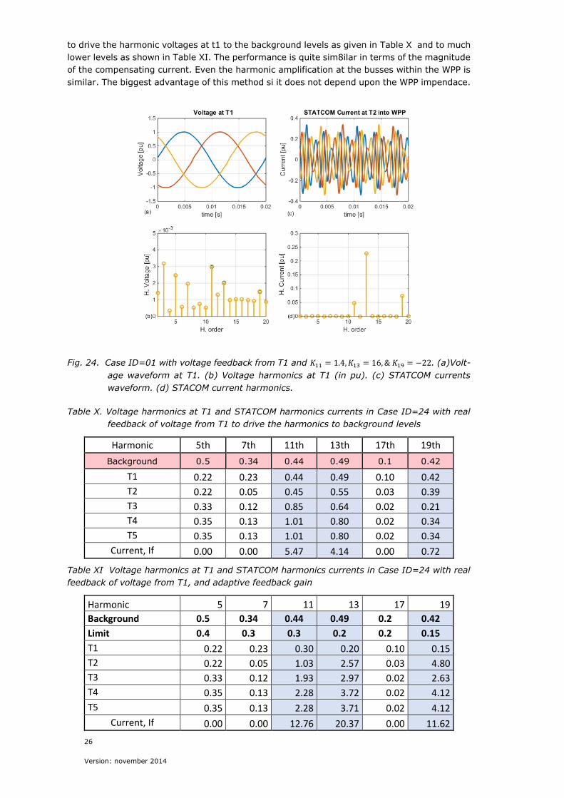
to drive the harmonic voltages at t1 to the background levels as given in Table X and to much

lower levels as shown in Table XI. The performance is quite sim8ilar in terms of the magnitude

of the compensating current. Even the harmonic amplification at the busses within the WPP is

similar. The biggest advantage of this method si it does not depend upon the WPP impendace.

Fig. 24. Case ID=01 with voltage feedback from T1 and 𝐾11 = 1.4, 𝐾13 = 16, & 𝐾19 = −22. (a)Volt-

age waveform at T1. (b) Voltage harmonics at T1 (in pu). (c) STATCOM currents

waveform. (d) STACOM current harmonics.

Table X. Voltage harmonics at T1 and STATCOM harmonics currents in Case ID=24 with real

feedback of voltage from T1 to drive the harmonics to background levels


Background 0.5 0.34 0.44 0.49 0.1 0.42

T1 0.22 0.23 0.44 0.49 0.10 0.42

T2 0.22 0.05 0.45 0.55 0.03 0.39

T3 0.33 0.12 0.85 0.64 0.02 0.21

T4 0.35 0.13 1.01 0.80 0.02 0.34

T5 0.35 0.13 1.01 0.80 0.02 0.34

Current, If 0.00 0.00 5.47 4.14 0.00 0.72

Table XI Voltage harmonics at T1 and STATCOM harmonics currents in Case ID=24 with real

feedback of voltage from T1, and adaptive feedback gain

Harmonic 5 7 11 13 17 19

Background 0.5 0.34 0.44 0.49 0.2 0.42

Limit 0.4 0.3 0.3 0.2 0.2 0.15

T1 0.22 0.23 0.30 0.20 0.10 0.15

T2 0.22 0.05 1.03 2.57 0.03 4.80

T3 0.33 0.12 1.93 2.97 0.02 2.63

T4 0.35 0.13 2.28 3.72 0.02 4.12

T5 0.35 0.13 2.28 3.71 0.02 4.12

Current, If 0.00 0.00 12.76 20.37 0.00 11.62

27


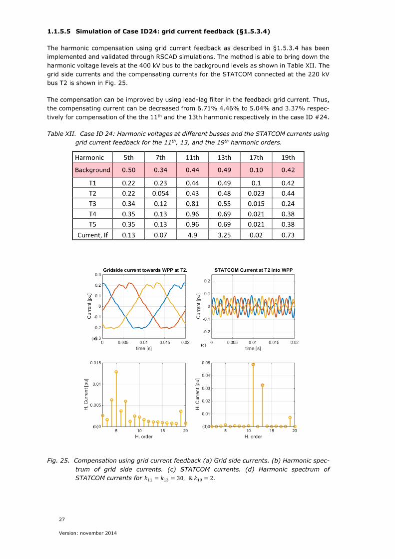
1.1.5.5 Simulation of Case ID24: grid current feedback (§1.5.3.4)

The harmonic compensation using grid current feedback as described in §1.5.3.4 has been

implemented and validated through RSCAD simulations. The method is able to bring down the

harmonic voltage levels at the 400 kV bus to the background levels as shown in Table XII. The

grid side currents and the compensating currents for the STATCOM connected at the 220 kV

bus T2 is shown in Fig. 25.

The compensation can be improved by using lead-lag filter in the feedback grid current. Thus,

the compensating current can be decreased from 6.71% 4.46% to 5.04% and 3.37% respec-

tively for compensation of the the 11th and the 13th harmonic respectively in the case ID #24.

Table XII. Case ID 24: Harmonic voltages at different busses and the STATCOM currents using

grid current feedback for the 11th, 13, and the 19th harmonic orders.


Background 0.50 0.34 0.44 0.49 0.10 0.42

T1 0.22 0.23 0.44 0.49 0.1 0.42

T2 0.22 0.054 0.43 0.48 0.023 0.44

T3 0.34 0.12 0.81 0.55 0.015 0.24

T4 0.35 0.13 0.96 0.69 0.021 0.38

T5 0.35 0.13 0.96 0.69 0.021 0.38

Current, If 0.13 0.07 4.9 3.25 0.02 0.73

Fig. 25. Compensation using grid current feedback (a) Grid side currents. (b) Harmonic spec-

trum of grid side currents. (c) STATCOM currents. (d) Harmonic spectrum of

STATCOM currents for 𝑘11 = 𝑘13 = 30, & 𝑘19 = 2.

28


1.1.5.6 Transient simulation of Case ID24 with complex feedback of voltage from

T1 (§1.5.3.1)

A series of switching transient events were created to observe the controller performance

and stability against the transient events. Also since some network component gets switched

off or on, this also indicates the robustness against some of the parameters to some extent.

The following events were simulated in sequence with random time interval between them.

A. Start simulation with everything connected

B. Turn on the compensator

C. Switch off one of the two 410/233 kV transformers

D. Switch off one of the three collector-bus transformers

E. Switch off the second collector-bus transformers

F. Switch off half of the collector feeder connected to the remaining transformer

G. Switch on one of the two 410/233 kV transformers

It was observed that the switching on/off of the 410/233 kV transformer had maximum impact

upon the harmonic voltage distortion at T1. Nevertheless, the compensator worked to mitigate

the disturbance and drive the harmonic voltage levels to the reference limit levels as shown in

Fig. 26. Other events like switching off/on the collector bus transformer, and the collector

feeders had negligible impact.

Fig. 26. Performance of the harmonic compensator during transformer switching transients.

29


1.1.5.7 Transient simulation of grid current feedback (§1.5.3.4)

The transient events listed in §1.1.5.6 were applied for the 16 cases with different values

of grid impedances. All the cases were find to be stable. Further, very fast stabilization of the

transients were observed after each of the switching events. The fast stabilization can be at-

tributed to the fact that the voltage harmonics at T1 settles to the background harmonic levels,

unlike very low harmonic voltage levels specified in the previous section (§1.1.5.6).

1.6. Utilization of project results

How do the project participants expect to utilize the results obtained in the project?

Do any of the project participants expect to utilize the project results - commercially or

otherwise? Which commercial activities and marketing results do you plan for? Has your

business plan been updated? Or a new business plan produced? What future context is the

end results expected to be part of, e.g. as part of another product, as the main product or

as part of further development and demonstration? What is the market potential/Compe-

tition?

The project was exploring application of active filter functionality embedded in STATCOMs

used in wind power plants. The outcome of the project led to significant increase of in-house

knowledge regarding advantages and challenges of active filtering. Furthermore during the

research project execution the first deliverables contributed to simultaneous first large-scale

demonstration of active filtering embedded in STATCOMs in a commercial large offshore wind

power plant. The demonstration, as well as the research project, appeared to be very success-

ful and opened next gates to commercial application of this technology in future commercial

projects.

Do project participants expect to take out patents?

The project participants do not expect to file any patent applications.

How do project results contribute to realize energy policy objectives?

The application of active filtering embedded in STATCOMs, especially in large offshore wind

power plants where STATCOMs are typically needed to fulfill demanding grid code requirement,

can potentially minimize development, capital and operating expenditures by reducing the

state-of-the-art passive filter size or completely removing the need for it, and consequently

reducing the cost of renewable electricity.

Have results been transferred to other institutions after project completion? If Ph.D.s

has been part of the project, it must be described how the results from the project are used

in teaching and other dissemination activities

Within the project a number of publications were released as a part of dissemination of

knowledge. They were used in communication with various internal and external stakeholders

in order to bring closer the concept of active filtering in wind power plants and initiate first

steps in commercial application supporting demonstration activities and tendering processes.

1.7. Project conclusion and perspective

Test grid model based on Anhiolt WPP has been developed in DigSILENT,

PSCAD and RSCAD. Harmonic impedance scan and powerflow analysis

analyses show similar behaviour in the three models, though there are differ-

ences.

30


24 Different grid impedance cases has been modelled in the form of frequency

dependent network equivalent using vector curve fitting and modelled in

PSCAD and RSCAD.

Resistive compensation at the 400 kV and 220 kV bus nearest to the onshore

grid has been analysed. It is concluded that such a compensation reduces the

harmonic voltage distortion at the local bus and downstream. The reduction is

not guaranteed on the upstream busses, there some cases there can be an am-

plification.

Four new methods for harmonic compensation have been proposed and two

of them have been investigated and validated through time domain simulations

in PSCAD and RSCAD. One of them is based upon voltage feedback, while

the other one is based upon current feedback.

It has been demonstrated that the harmonic amplification at the remote 400

kV bus can be limited to the background harmonic levels by providing com-

pensation at the 220 kV bus.

Moreover, it is possible to attenuate the harmonic voltages at the 400 kV bus

to levels lower than the background levels by providing compensation at the

220 kV bus. However, it increases the harmonic levels inside the WPP.

Dynamic simulation of the controller in the presence of switching events of

the grid transformer as well as the collector bus transformers has been carried

out to confirm the robustness of the controller.

Annex

Summary of the simulation results of the 16 different case (Grid impedance case ID#1 to

24 except the cases 6, 13, and 18 to 23)

A. Harmonic compensation method using T1 voltage feedback (§1.1.5.2), and the

feedback being complex transfer function.

B. Comparison of results with the complex (i.e. transfer function as described in

(§1.1.5.2) and real (i.e. proportional as described in §1.1.5.4) feedback of volt-

age at T1.

C. Harmonic compensation method using real (proportional) feedback of grid

current (§1.5.3.4)

Documents

Th - Energiteknologi · Project title Active filter functionalities for power converters in wind power plants Project identification (pro-gram abbrev. and file) 12188 Name of the