Activity Tracking with IoT and accelerometers Alejandro Iñigo Córdoba / aio600 / March 21th of 2018

Abstract- Increasingly, PyCom technology is used to create a wearable device which count steps [1] and send them to the The Things Network (TTN). How to implement a step counter on a PyCom device and how to configure the LoRaWAN network to send data to the TTN are the major challenges. The aim of this research is to study the feasibility of a LoraWAN connected activity tracker/step counter. In this paper, I have developed a Micropython step counter algorithm that facilitates the programming of PyCom devices to other users. In addition, in this work I investigate the communication between PyCom and TTN. Existent Python step counter code is transformed into a Micropython one and the communication with the TTN is implemented using Atom. I show that this process is possible, but it is needed a LoPy PyCom device with a bigger memory.

I. INTRODUCTION

PyCom technology is used to create a wearable device which count steps and send them to the TTN. The most usable information found to do this is in the official pyCom device webpage [2]. A LoPy1.0r multipack, which include a LoPy1.0r, an Expansion Board and a LoRa/Sigfox antenna is used for this project. Even though, the project is focused on software, not on hardware (my task was the implementation of the software or a working system in Micropython language that can track the steps of a person wearing the device and send those to the TTN).

The major challenges are how to implement a step counter on a pyCom device and how to configure the LoRaWAN network to send data to the TTN. The step counter algorithm is complex: it includes mathematical and physical methods like linear interpolation or programming techniques like Threads or Queues. Using the code explained in the chapter related work [3], a Micropython code was created based on it. After this code is created and is working on the device, the steps which are the output of this algorithm are sent to the TTN. This sending is also implemented in this language.

The goals of my research are to study the feasibility of a LoraWAN connected activity tracker/step counter. To do this is necessary to make a working system that can track the steps of a person wearing the device. “Is it possible to generate a step counter algorithm in Micropython and introduce this into the LoPy pyCom device?”, “Is it possible to connect the activity tracker/step counter with the TTN and send the steps generated in the previous question?”. These questions will be explained in detail in the chapter ii bellow.

In this paper, my contribution to the society with this project is a Micropython step counter algorithm that facilitates the programming of pyCom devices to other users, as well as the communication between them and the TTN. We show the feasibility of the proposed method, the implementation of PyCom based’ step counter and the sending of the steps to the TTN. This is an open-source project, therefore can be used by individuals and/or organization who are interested in developing pedometer apps.

The process that I followed to conclude with this project starts with (1) understanding an existent Python step counter code, mentioned previously and explained in the chapter iv. In the next step, the Python algorithm is

(2) transformed into a MicroPython one explained in the subchapter iii-h investigating about APIs and related modules between these two languages. The code generated in Micropython (3) is introduced in a LoPy PyCom device, more concretely a LoPy1.0r using a program called Atom. After the code has been generated and the steps calculated, these steps were sent to the TTN. For this, it was necessary first to (4) investigate about how to use the platform “The Things Network” [4]. After that it wasimportant to know more about (5) Micropython code to communicate the device with this platform and then being able to send these steps to this TTN.

The structure is composed by eight main chapters: (1) abstract, (2) introduction, (3) research question, (4) body, (5) related work, (6) conclusion, (7) appendix and (8) bibliography:

The abstract contains the problem discussed in the paper plus my own contribution. The (i) introduction tells the complete story: the structure of this is composed by a context (discussion of the problem area), the problem identification (the problem that is (partly) solved in this paper), the objective of the research (the goals), an indication of the solution (direction) or contribution, what method was used and an explanation of the structure of the paper. The (ii) research questions chapter explains the main questions that are answered in this paper and why they were chosen. (iii) Body contains the content of the project in detail. In this paper, this is composed by the subsections:

a. The internet of things.b. Step counter or pedometer.c. LoRa and LoRaWANd. LoPy1.0. e. Windowed peak detection and its stages.f. The signal representation: example case.g. Linear interpolation.h. From Python to Micropython.i. Garbage collector.j. Connection with the TTN.

The (iv) related work chapter contains references to other research projects that have been useful to the implementation of this one. This can serve two purposes: summarizing the work of others or positioning my work in relation to work of others. The (v) conclusion summarizes and suggests further research, the contribution and findings, an outlook on future work/remaining problems (this section motivate other researchers to participate in my area).

II. RESEARCH QUESTIONS

For the execution of this project, two main questions have been answered. These questions haven’t been suggested by the student, but they were imposed by the supervisor. These questions are:

A. How to create a step counter on the PyComdevice?

This is the first question imposed. To do this, it is not necessary to be focused on the hardware, but it is to be focused on the algorithm of a step counter. Being sure that every stage of the Windowed Peak Detection (WPD) is clear is the first step. For this task it is used the report “Step Counter Algorithm for smartphones organization” referenced in the chapter i. From this report an algorithm in Python is taken and then it is possible to start working. This is explained in more detail in the chapter iv. The output of this program is the number of steps that the user who is wearing the device walks. Once the algorithm is clear, the main task is to transform the Pycom code into a Micropython one and then to introduce this in the PyCom device (precisely the LoPy1.0r) using the program Atom and a LoPy1.0r multipack with several changes and contributions.

B. How to configure the LoRaWAN network to send step data to the TTN?

This is the second question imposed. To answer this question, it is important to know well the platform TheThingsNetwork referenced previously. This platform is used for building networks for the Internet of Things by using LoRaWAN technology, which doesn’t use 3G or WiFi, uses low battery, long range and low bandwidth. After this is known it is necessary to create an account, to create an application and a device in this platform. Once it is created some code must be implemented in Atom to connect the device LoPy1.0r with this platform. This code is added to the previously created code (first question) and the output of the first question (number of steps) is sent to the Internet of Things (TTN). This process is explained in more detail in the chapter iii-j.

III. BODY

Before starting with the explanation of what has been done during the implementation of this project, it is important to understand general concepts like the Internet of Things (IoT), the LoRa technology, LoRaWAN protocol and what is a step counter or pedometer. The first thing that is going to be shown in this paper is what do these concepts mean and what is the relation between them.

A. The internet of things

Internet of Things (IoT) is a concept that is referred to the digital connection of daily objects using the Internet. This idea was proposed by Kevin Ashton in the MIT Autor-ID Center in 1999, where research in the Radio Frequency Identification (RFID) field and sensors technologies were carried out. The Gartner company predict that for 2020 will be approximately 26 thousand millions of wireless devices connected by The Internet and Abi Research 30 thousand million. In the future the IPV6(next generation of applications in the Internet) will allow us to identify all those devices. These are connected to the network by using low power radio signals (more active research field of the IoT) and they don’t need WiFi or Bluetooth. The Alcatel-Lucent service touchatag and the Violeta Mirror gadget offer a pragmatic orientation to the IoT consumers, where everyone can link real world elements with the online world using tags like RDIF or QR codes. As the IoT research is in a very early development, there is not a standard definition of this term.

In this project a PyCom device is being used as an IoT device (more details about the device are in chapter iii-d). This device takes acceleration data by using sensors. The Windowed Peak Detection (WPD) algorithm (explained in the chapter iii-e) is implemented in this device (explained in the chapter iii-h) to obtain the steps from the acceleration data. After the steps are calculated, this information is sent to the TTN (explained in the chapter iii-j).

B. Step counter or pedometer

Before starting with the previously mentioned explanations, it is important to know more about what a step counter is.

1 Description and usage

A pedometer is an electronic device that counts the steps that a person walks by the use of sensors, and thus it records the kilometers or miles (distance = number of steps x step length). These devices are very common in sport players. These devices are not only used to count steps,

it is also useful for motivating fitness enthusiasts. Step counters can cheer up to complete with oneself in getting fit and losing weight. Nowadays, the software that these pedometers use determines automatically the variation of the person’s steps (the distance traveled can be measured directly by a GPS receiver). Step counters are being integrated into an increasing number of portable consumer electronic devices such as music players or smartphones. Various websites exist to allow people to track their progress. Pedometers have been shown in clinical studies to increase physical activity and reduce blood pressure levels and Body Mass Index [5]. One criticism of the pedometer is that it does not record intensity, but this can be done by making step goals time limited (for example, 1000 steps in 10 minutes counts as moderate exercise).

2 Technology

The step counter includes a mechanical sensor and a software to count steps. Nowadays pedometers rely on MEMS (Microelectromechanical Systems), inertial sensors and sophisticated software to detect steps. The sensors are very simple. The power consumption is low and the temperature is stable. To compensate for angular shock and vibration in the disk it is used these MEMS angular acceleration. These sensors have either 1, 2 or 3-axis detection of acceleration. The 2-axis accelerometers measure the dynamic acceleration or vibration and the static acceleration or gravity. The output of these step counters are signals which can be analog or digital. These are cycle modulated signals. The use of these inertial sensors permits more accurate detection of steps and fewer false positives. Pedometers have to be accurate. The software technology used to interpret the output of the inertial sensor and "make sense of accurate steps" varies widely.

C. LoRa and loRaWAN

As well as it is important to know about what a step counter or pedometer is, it is also important to know about what is loRa and loRaWAN. These will be use later to connect our device with the TTN.

1. LoRa and IoT

The construction of IoT networks are a common practice to send information to the TTN. LoRa is one of the most used long range, low power wireless platform to this commitment. The IoT, as we explained previously in the chapter iii-a, is improving the interaction between people and making many other improvements in society like climate change aspects, pollution or warning of natural disasters. IoT is also helping business in their operations and reduction of costs. Wireless radio frequency (RF) is needed to this communication, that’s why it is more often being integrated into vehicles, public lights, manufacturing equipment, etc.

2. LoRa technology

This is a more specific description of the used technology for data transmission with the TTN. This technology offers long range, security and makes the consumption of power low. Existing cellular networks provide a lower range in coverage than the networks which use this technology. This technology is more and more being introduced in chipsets by companies like Semtech [6] and these chipsets are then integrated into their products and into wireless telecommunication wide area networks (long range communications), Low-Power and Wide-Area Networks (LPWAN).

3. LoRaWAN protocol

This protocol is used together with LoRa technology. The developers of this protocol are LoRa Alliance [7]. This protocol enables low power, and wide area communications. This is why it is used unlicensed radio spectrum in the Industrial Scientific and Medical (ISM) bands. This protocol or standard allows for a quick, bidirectional and secure setup of networks. This also provides accurate location.

4. Key features of LoRa and LoRaWAN

LoRa and LoRaWAN are characterized for using geolocation and the cost of these is low because it reduces costs in different ways. The fact that these are standardized improve interoperability. The needed power is not high (battery lifetime up to twenty years), the range is long, it allows

penetration in dense urban and indoor regions and it also connects in rural areas up to thirty miles away. About the security, it uses end-to-end encryption and about the capacity, it supports millions of messages.

D. LoPy1.0

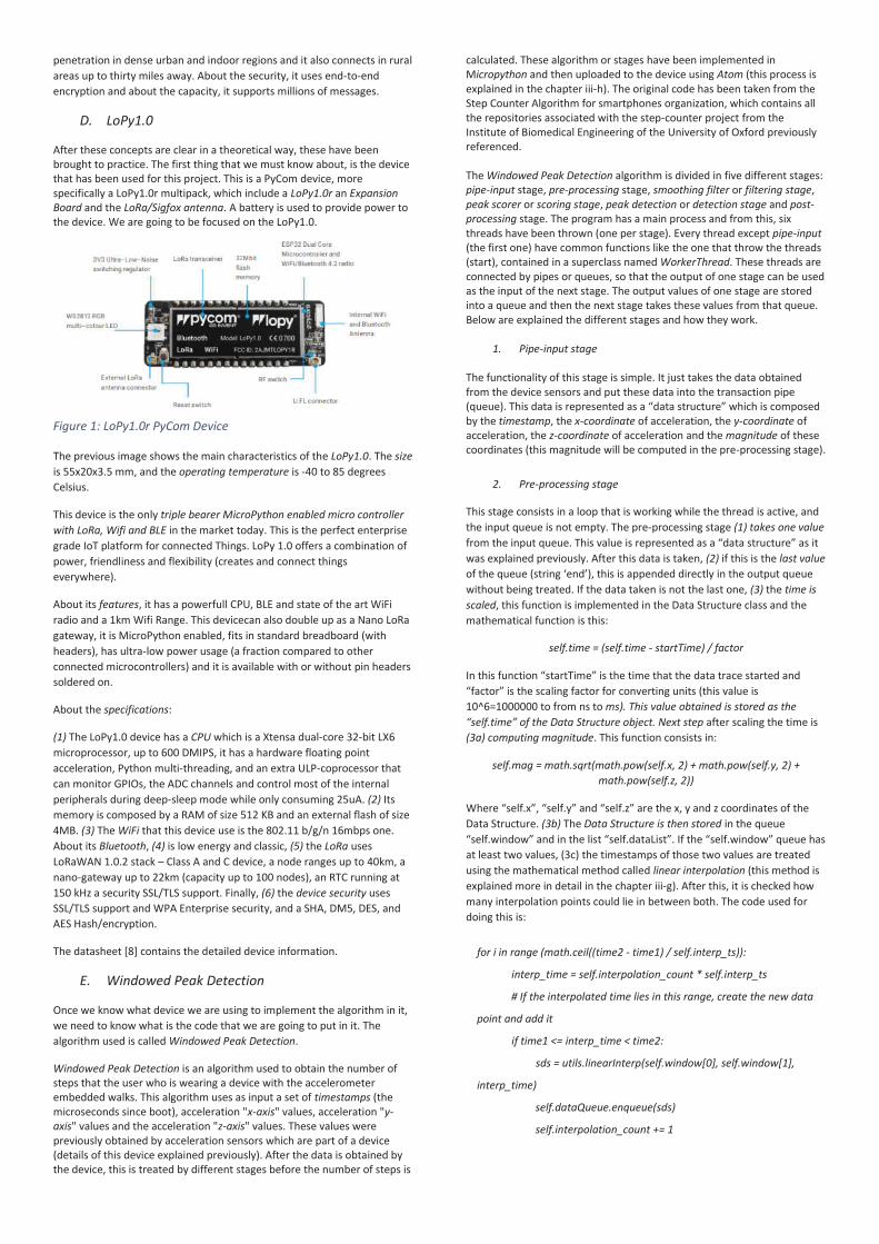
After these concepts are clear in a theoretical way, these have been brought to practice. The first thing that we must know about, is the device that has been used for this project. This is a PyCom device, more specifically a LoPy1.0r multipack, which include a LoPy1.0r an Expansion Board and the LoRa/Sigfox antenna. A battery is used to provide power to the device. We are going to be focused on the LoPy1.0.

Figure 1: LoPy1.0r PyCom Device

The previous image shows the main characteristics of the LoPy1.0. The size is 55x20x3.5 mm, and the operating temperature is -40 to 85 degrees Celsius.

This device is the only triple bearer MicroPython enabled micro controller with LoRa, Wifi and BLE in the market today. This is the perfect enterprise grade IoT platform for connected Things. LoPy 1.0 offers a combination of power, friendliness and flexibility (creates and connect things everywhere).

About its features, it has a powerfull CPU, BLE and state of the art WiFi radio and a 1km Wifi Range. This devicecan also double up as a Nano LoRa gateway, it is MicroPython enabled, fits in standard breadboard (with headers), has ultra-low power usage (a fraction compared to other connected microcontrollers) and it is available with or without pin headers soldered on.

About the specifications:

(1) The LoPy1.0 device has a CPU which is a Xtensa dual-core 32-bit LX6 microprocessor, up to 600 DMIPS, it has a hardware floating point acceleration, Python multi-threading, and an extra ULP-coprocessor that can monitor GPIOs, the ADC channels and control most of the internal peripherals during deep-sleep mode while only consuming 25uA. (2) Its memory is composed by a RAM of size 512 KB and an external flash of size 4MB. (3) The WiFi that this device use is the 802.11 b/g/n 16mbps one. About its Bluetooth, (4) is low energy and classic, (5) the LoRa uses LoRaWAN 1.0.2 stack – Class A and C device, a node ranges up to 40km, a nano-gateway up to 22km (capacity up to 100 nodes), an RTC running at 150 kHz a security SSL/TLS support. Finally, (6) the device security uses SSL/TLS support and WPA Enterprise security, and a SHA, DM5, DES, and AES Hash/encryption.

The datasheet [8] contains the detailed device information.

E. Windowed Peak Detection

Once we know what device we are using to implement the algorithm in it, we need to know what is the code that we are going to put in it. The algorithm used is called Windowed Peak Detection.

Windowed Peak Detection is an algorithm used to obtain the number of steps that the user who is wearing a device with the accelerometer embedded walks. This algorithm uses as input a set of timestamps (the microseconds since boot), acceleration "x-axis" values, acceleration "y-axis" values and the acceleration "z-axis" values. These values were previously obtained by acceleration sensors which are part of a device (details of this device explained previously). After the data is obtained by the device, this is treated by different stages before the number of steps is

calculated. These algorithm or stages have been implemented in Micropython and then uploaded to the device using Atom (this process is explained in the chapter iii-h). The original code has been taken from the Step Counter Algorithm for smartphones organization, which contains all the repositories associated with the step-counter project from the Institute of Biomedical Engineering of the University of Oxford previously referenced. The Windowed Peak Detection algorithm is divided in five different stages: pipe-input stage, pre-processing stage, smoothing filter or filtering stage, peak scorer or scoring stage, peak detection or detection stage and post-processing stage. The program has a main process and from this, six threads have been thrown (one per stage). Every thread except pipe-input (the first one) have common functions like the one that throw the threads (start), contained in a superclass named WorkerThread. These threads are connected by pipes or queues, so that the output of one stage can be used as the input of the next stage. The output values of one stage are stored into a queue and then the next stage takes these values from that queue. Below are explained the different stages and how they work.

1. Pipe-input stage

The functionality of this stage is simple. It just takes the data obtained from the device sensors and put these data into the transaction pipe (queue). This data is represented as a “data structure” which is composed by the timestamp, the x-coordinate of acceleration, the y-coordinate of acceleration, the z-coordinate of acceleration and the magnitude of these coordinates (this magnitude will be computed in the pre-processing stage).

2. Pre-processing stage

This stage consists in a loop that is working while the thread is active, and the input queue is not empty. The pre-processing stage (1) takes one value from the input queue. This value is represented as a “data structure” as it was explained previously. After this data is taken, (2) if this is the last value of the queue (string ‘end’), this is appended directly in the output queue without being treated. If the data taken is not the last one, (3) the time is scaled, this function is implemented in the Data Structure class and the mathematical function is this:

self.time = (self.time - startTime) / factor

In this function “startTime” is the time that the data trace started and “factor” is the scaling factor for converting units (this value is 10^6=1000000 to from ns to ms). This value obtained is stored as the “self.time” of the Data Structure object. Next step after scaling the time is (3a) computing magnitude. This function consists in:

self.mag = math.sqrt(math.pow(self.x, 2) + math.pow(self.y, 2) + math.pow(self.z, 2))

Where “self.x”, “self.y” and “self.z” are the x, y and z coordinates of the Data Structure. (3b) The Data Structure is then stored in the queue “self.window” and in the list “self.dataList”. If the “self.window” queue has at least two values, (3c) the timestamps of those two values are treated using the mathematical method called linear interpolation (this method is explained more in detail in the chapter iii-g). After this, it is checked how many interpolation points could lie in between both. The code used for doing this is:

for i in range (math.ceil((time2 - time1) / self.interp_ts)):

interp_time = self.interpolation_count * self.interp_ts

# If the interpolated time lies in this range, create the new data

point and add it

if time1 <= interp_time < time2:

sds = utils.linearInterp(self.window[0], self.window[1],

interp_time)

self.dataQueue.enqueue(sds)

self.interpolation_count += 1

Where ‘’inter_ts’’ is defined as 10 and represent the interpolation time scale in ms. “Interpolation_count” is initialized as 0 in the constructor of the class and it is adding 1 at each iteration. The values “time1” and “time2” are the first and the second values in the “self.window” queue. The linear interpolation function returns a Simple Data Structure where time is the “interp_time” and the new magnitude is calculated as:

new_mag = slope* (time – time1) + value1

In this function “time” is the interpolation time (interp_time), “time1” is the time of the first data structure, “value1” is the magnitude of the first data structure and “slope” is:

slope = (value2 – value1) / (time2 – time1)

To conclude, (3d) as we can see in the previous code, these interpolation points are stored in the output queue as Simple Data Structures.

3. Filtering stage

Different filters can be applied for this stage: the Hann Filter, the Gaussian Filter, the Kaiser Bessel Filter or the Centered Moving Average Filter. When this program is executed, the filter is specified previously. All of them are implemented but only one can be executed at a time. The one that we are going to execute first is the Gaussian Filter.

Before starting treating any data, the Gaussian window coefficients are generated, this is a list that contain values which are the result of a mathematical expression. This is:

value = math.exp(-0.5 * math.pow((n – (windowSize - 1) / 2) / (std * windowSize - 1) / 2), 2))

where “windowSize” is the size of the Gaussian Window, in our case we use 13 and “std” is the adjusted standard deviation, we are using 0.35.

Once it is done, while the thread is active, the filtering stage (1) takes data from the queue or pipe where the previous stage stored its output and while there are data in the queue. These data are the interpolation points which are represented as a simple data structure (that is composed by the timestamp, the magnitude of the signal and the old magnitude as class attributes), (2) If the last value of the pipe is being taken (the string ‘’end”), then this value is not treated, and it is directly added to the output queue and the thread is done (completed and not active). (3) If the data taken from the input queue is a regular simple data structure, this is stored in a list called “data” and in a queue called “window”. (3a) If the size of ‘’window’’ is equals to ‘’windowSize’’ (13 as we saw before), then the smoothing action is done and then pop operation is performed. The smoothing action consist in the next code:

ssum = 0 for i in range(len(self.window)): ssum += self.window[i].mag * self.gauss_window[i]

The ‘’gauss_window’’ is the list that contain the values ‘’values’’ that we also saw before and “self.window[i].mag” is the magnitude of the position “i” of the queue “self.window”.

To conclude with this stage, (3b) the data that is going to be appended as a simple data structure in the output queue is the average of all points in the window.

4. Scoring stage

As well as for the previous stage (filtering stage), different functions have been implemented but only one is executed each time. These functions are: Pass-through scoring, Maximum Difference scoring, Mean Difference scoring and Pan-Tompkins scoring. When the code is executed the scoring function is specified previously, and the one that we are focusing on is Mean Difference scoring.

This scoring function is a loop that is iterating while the thread is active and there is data in the input queue. The first step in this stage is (1) taking the first value of the input queue which was previously appended in the

Filtering Stage as a Simple Data Structure. (2) If the value taken is the last one (the string “end”), this is directly appended in the output value and thread is over (completed and not active). If the data taken is not the last one, (3) this Simple Data Structure is appended in a list called “self.data” and ‘’self.window’’ as well as in the previous stage. If the size of the “self.window” queue is equals to the window size (it was previously declared as 35), (3a) the mean of the window is calculated using the code:

ssum = 0 for i in range(0, self.windowSize):

ssum += self.window[i].mag mean = ssum / self.windowSize

In this code “self.windowSize” is 35 as we said before, and the “self.window[i].mag” is the magnitude of the Simple Data Structure of the position “i” in the queue “self.window”.

After this, (3b) the new magnitude is calculated with the code:

new_mag = 0 if self.window[midPoint].mag–mean < 0 else self.window[midPoint].mag - mean # Square it new_mag *= new_mag

In this code “midPoint” is the “windowSize” divided by 2 (this is int (17,5)=17) and “mean” was calculated previously. The new magnitude is 0 if the difference between the magnitude of the 17th point and the previously calculated mean is less than 0 and if this is not, then the new magnitude is that difference. After that is squared.

To conclude, (3c) the new data appended to the output queue is a Simple Data Structure with the time of the 17th value of “self.window”, the new magnitude calculated previously and the old magnitude.

5. Detection stage

This stage consists in a loop that is iterating while the thread is running, and while the input queue has values in it. The first step that this stage does is (1) taking the first value of the queue. This value had been added to the output queue of the last stage as a Simple Data Structure. If this value is the last one of the queue (the string “end”) (2) then this is directly appended into the output queue and the thread is over (completed and not active). If this value is not the last one, (3) this is appended to a list called “self.data”. This stage consists in using a simple mean and standard deviation method to find significant values of peak scores from the values obtained in the previous stage. That is why the algorithm does the next: Before explaining the update statistics method is important to say that “self.n”, “self.mean” and “self.std” were previously initialized to 0 in the constructor before throwing the thread and this values are the internal statistics. One is summed to “self.n”, if “self.n” is now 1, (3a) “self.mean” is now the magnitude of the Simple Data Structure taken from the input queue and “self.std” is still 0. If “self.n” is now 2, “self.mean” is now the average between the magnitude of the Simple Data Structure taken and the actual “self.mean” and “self.std” is:

self.std = math.sqrt((math.pow(dp.mag - self.mean, 2) + math.pow(o_mean - self.mean, 2)) / 2)

Where “dp.mag” is the magnitude of the Simple Data Structure taken, “self.mean” is the one obtained in the last step and “o_mean” is the “self.mean” before the last step.

If “self.n” is not 1 or 2, then (3b) the mean iteratively is updated like this:

self.mean = (dp.mag + (self.n - 1) * self.mean) / self.n

And the standard deviation like this:

std = math.sqrt(((self.n - 2) * math.pow(self.std, 2) / (self.n - 1)) + math.pow(o_mean - self.mean,2) + math.pow(dp.mag - self.mean, 2) / self.n)

What each value means was already explained previously.

The last step in this stage is (3c) If “self.n” is bigger than 15, to check if we are above the threshold. This threshold has been defined as “1.2”. If the difference between the magnitude of the Simple Data Structure obtained from the input queue and the actual value “self.mean” is bigger than the product between “self.std” and “1.2” (threshold), then a Simple Data Structure with the time of the Simple Data Structure obtained from the input queue and also its old magnitude is appended to the output queue and also to the list “self.dataout”.

6. Post-processing stage

This is the last stage of the Windowed Peak Detection. This consist in a loop that is running while the thread is active, and the input queue has values in it. If these two conditions are satisfied, then (1) the first value of the input pipe is taken (this is a Simple Data Structure). (2) If this first structure is the last one from the queue (the string ‘’end’’), then the last value from the internal queue “self.queue” is taken, and this is appended into the output list. Also, the thread is done (completed and not active). If the Simple Data Structure taken from the input queue is not the last one, then (3) if the internal queue “self.queue” size is less than 2, then the SDS is appended. If not (3a), if the time difference (this is the difference between the time of the SDS taken from the input queue and the time of the SDS that is in the first position of the internal queue) is bigger than the threshold (this value has been defined previously as 200), then the old point is popped from the internal queue (“self.queue”), this is appended to the output queue and the new point (SDS from input queue) is appended to the internal queue “self.queue”. In the case that this difference of time is not bigger than the threshold, (3b) if the magnitude of the SDS taken is bigger or equals than the first value magnitude of the internal queue “self.queue”, then the actual value in this queue is popped and the new SDS from the input pipe is appended (it is only kept the maximum value point).

F. The signal representation: example case

The algorithm is already explained, now it is shown a signal representation of the data at the output of every stage for a specific example:

In this example, the next values are used:

For (1) pre-processing stage, it is used as interpolation time scale in milliseconds (“inter_ts”) and time scale factor (“ts_factor”) 100 and 1000000 respectively. For (2) filtering stage, it is executed the “Smoothing filter” and it is used as size of the filter window (“windowSize”) and as standard deviation (“std”) 51 and 0.35 respectively. For (3) scoring stage, it is executed the “Mean difference scoring” and it is used as scoring size of the window (“windowSize”) 10. For (4) detection stage, it is used as the standard deviation threshold to call a peak a peak (“threshold”) 1.2. And finally, for (5) post-processing stage, it is used as time threshold for eliminating peaks (“time_threshold”) 200 milliseconds.

The next images have been obtained from the report “An optimized algorithm for accurate steps counting from smart-phone accelerometry” previously referenced and are represented each stage values for this example.

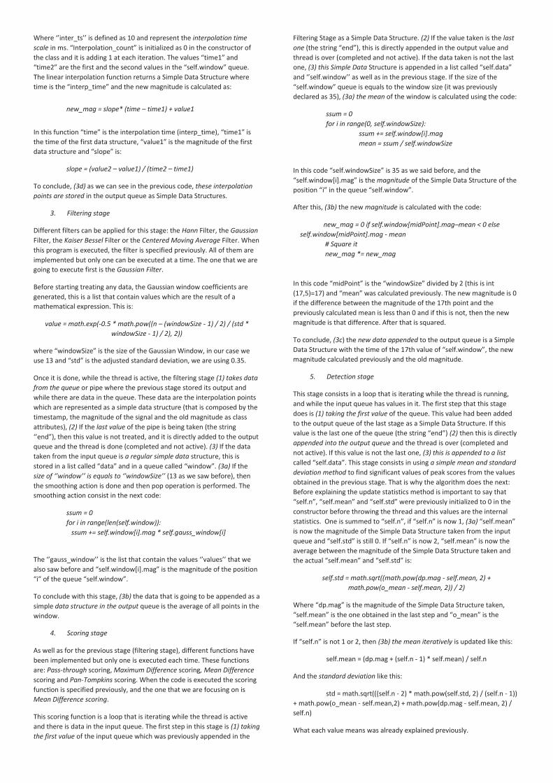
1. Pipe-input stage

This signal represents in the x-axis the samples from 0 to 1500 and in the y-axis the difference in time between those in milliseconds. In this image can be seen that this difference is always around 10 milliseconds but there are clear desviations.

Figure 2: Pipe-input data representation.

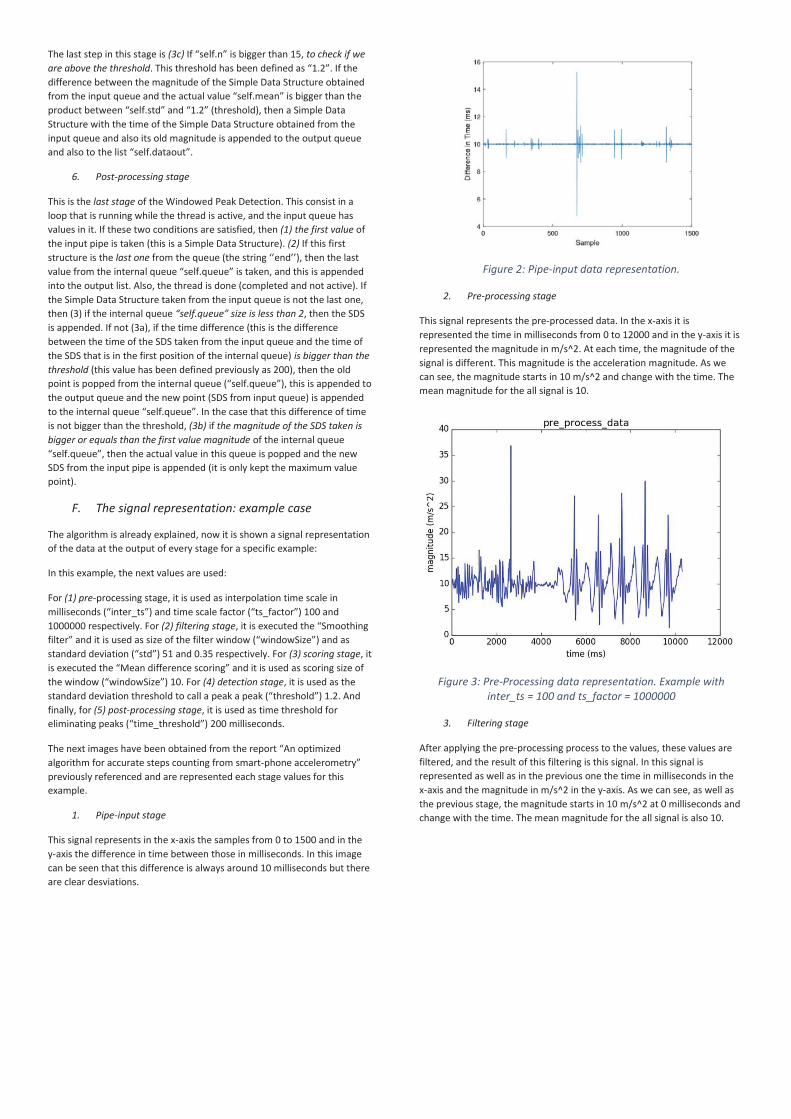
2. Pre-processing stage

This signal represents the pre-processed data. In the x-axis it is represented the time in milliseconds from 0 to 12000 and in the y-axis it is represented the magnitude in m/s^2. At each time, the magnitude of the signal is different. This magnitude is the acceleration magnitude. As we can see, the magnitude starts in 10 m/s^2 and change with the time. The mean magnitude for the all signal is 10.

Figure 3: Pre-Processing data representation. Example with

inter_ts = 100 and ts_factor = 1000000

3. Filtering stage

After applying the pre-processing process to the values, these values are filtered, and the result of this filtering is this signal. In this signal is represented as well as in the previous one the time in milliseconds in the x-axis and the magnitude in m/s^2 in the y-axis. As we can see, as well as the previous stage, the magnitude starts in 10 m/s^2 at 0 milliseconds and change with the time. The mean magnitude for the all signal is also 10.

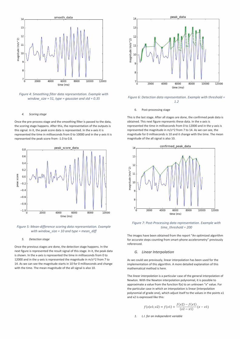
Figure 4: Smoothing filter data representation. Example with

window_size = 51, type = gaussian and std = 0.35

4. Scoring stage

Once the pre-process stage and the smoothing filter is passed to the data, the scoring stage happens. After this, the representation of the outputs is this signal. In it, the peak score data is represented. In the x-axis it is represented the time in milliseconds from 0 to 10000 and in the y-axis it is represented the peak score from -1.0 to 0.8.

Figure 5: Mean-difference scoring data representation. Example

with window_size = 10 and type = mean_diff

5. Detection stage

Once the previous stages are done, the detection stage happens. In the next figure is represented the result signal of this stage. In it, the peak data is shown. In the x-axis is represented the time in milliseconds from 0 to 12000 and in the y-axis is represented the magnitude in m/s^2 from 7 to 14. As we can see the magnitude starts in 10 for 0 milliseconds and change with the time. The mean magnitude of the all signal is also 10.

Figure 6: Detection data representation. Example with threshold =

1.2

6. Post-processing stage

This is the last stage. After all stages are done, the confirmed peak data is obtained. This next figure represents these data. In the x-axis is represented the time in milliseconds from 0 to 12000 and in the y-axis is represented the magnitude in m/s^2 from 7 to 14. As we can see, the magnitude for 0 milliseconds is 10 and it change with the time. The mean magnitude of the all signal is also 10.

Figure 7: Post-Processing data representation. Example with

time_threshold = 200

The images have been obtained from the report “An optimized algorithm for accurate steps counting from smart-phone accelerometry” previously referenced.

G. Linear Interpolation

As we could see previously, linear interpolation has been used for the implementation of this algorithm. A more detailed explanation of this mathematical method is here.

The linear interpolation is a particular case of the general interpolation of Newton. With the Newton interpolation polynomial, it is possible to approximate a value from the function f(x) to an unknown “x” value. For the particular case in which an interpolation is linear (interpolation polynomial of grade one), which adjust itself to the values in the points x1 and x2 is expressed like this:

1. L.I. for an independent variable

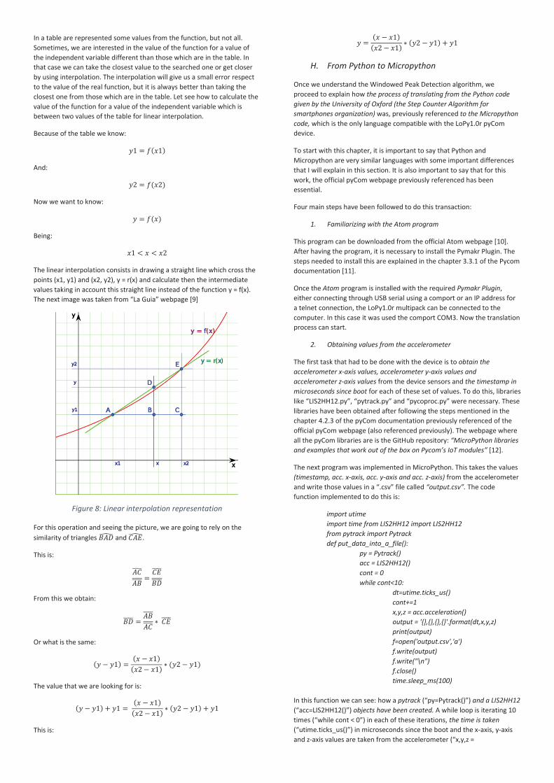
In a table are represented some values from the function, but not all. Sometimes, we are interested in the value of the function for a value of the independent variable different than those which are in the table. In that case we can take the closest value to the searched one or get closer by using interpolation. The interpolation will give us a small error respect to the value of the real function, but it is always better than taking the closest one from those which are in the table. Let see how to calculate the value of the function for a value of the independent variable which is between two values of the table for linear interpolation.

Because of the table we know:

And:

Now we want to know:

Being:

The linear interpolation consists in drawing a straight line which cross the points (x1, y1) and (x2, y2), y = r(x) and calculate then the intermediate values taking in account this straight line instead of the function y = f(x). The next image was taken from “La Guia” webpage [9]

Figure 8: Linear interpolation representation

For this operation and seeing the picture, we are going to rely on the similarity of triangles and .

This is:

From this we obtain:

Or what is the same:

The value that we are looking for is:

This is:

H. From Python to Micropython

Once we understand the Windowed Peak Detection algorithm, we proceed to explain how the process of translating from the Python code given by the University of Oxford (the Step Counter Algorithm for smartphones organization) was, previously referenced to the Micropython code, which is the only language compatible with the LoPy1.0r pyCom device.

To start with this chapter, it is important to say that Python and Micropython are very similar languages with some important differences that I will explain in this section. It is also important to say that for this work, the official pyCom webpage previously referenced has been essential.

Four main steps have been followed to do this transaction:

1. Familiarizing with the Atom program

This program can be downloaded from the official Atom webpage [10]. After having the program, it is necessary to install the Pymakr Plugin. The steps needed to install this are explained in the chapter 3.3.1 of the Pycom documentation [11].

Once the Atom program is installed with the required Pymakr Plugin, either connecting through USB serial using a comport or an IP address for a telnet connection, the LoPy1.0r multipack can be connected to the computer. In this case it was used the comport COM3. Now the translation process can start.

2. Obtaining values from the accelerometer

The first task that had to be done with the device is to obtain the accelerometer x-axis values, accelerometer y-axis values and accelerometer z-axis values from the device sensors and the timestamp in microseconds since boot for each of these set of values. To do this, libraries like “LIS2HH12.py”, “pytrack.py” and “pycoproc.py” were necessary. These libraries have been obtained after following the steps mentioned in the chapter 4.2.3 of the pyCom documentation previously referenced of the official pyCom webpage (also referenced previously). The webpage where all the pyCom libraries are is the GitHub repository: “MicroPython libraries and examples that work out of the box on Pycom’s IoT modules” [12].

The next program was implemented in MicroPython. This takes the values (timestamp, acc. x-axis, acc. y-axis and acc. z-axis) from the accelerometer and write those values in a “.csv” file called “output.csv”. The code function implemented to do this is:

import utime import time from LIS2HH12 import LIS2HH12 from pytrack import Pytrack def put_data_into_a_file():

py = Pytrack() acc = LIS2HH12() cont = 0 while cont<10:

dt=utime.ticks_us() cont+=1 x,y,z = acc.acceleration() output = '{},{},{},{}'.format(dt,x,y,z) print(output) f=open('output.csv','a') f.write(output) f.write("\n") f.close() time.sleep_ms(100)

In this function we can see: how a pytrack (“py=Pytrack()”) and a LIS2HH12 (“acc=LIS2HH12()”) objects have been created. A while loop is iterating 10 times (“while cont < 0”) in each of these iterations, the time is taken (“utime.ticks_us()”) in microseconds since the boot and the x-axis, y-axis and z-axis values are taken from the accelerometer (“x,y,z =

acc.acceleration”). To conclude, the obtained values (timestamp, accelerometer x, y and z values) are printed into a file which is created the first iteration and open the next 9 (“f=open(´output.csv´,’a’)”, “f.write(output)”, f.write(“/n”)” and “f.close()”). To conclude, every iteration happens after waiting 100 miliseconds (“time.sleep_ms(100)”).

3. Making sure that the file is correctly created

The created file is now stored in a small internal file system accessible from each PyCom Device which is called “/flash”. When the device starts up it always boot from the “boot.py” located in the “/flash” file system. The file system is accessible via the native FTP server running on each Pycom device. The file “boot.py” of this project has been modified, so that the device is being connected to a specific router (for example a personal home WiFi router). Now that this connection is done, and the file has been created, we can access to this server and this file by opening an FTP client. In this case, FileZilla client was used. It was installed, open and the connection was done following the steps in chapter 1.3.5 of the pyCom documentation already referenced. Once the connection is done it is possible to obtain the file from the server and put it in your computer. When the file is in your computer, it can be open with a program that support “.csv” files like for example Microsoft Excel.

After doing all this process and opening the file, the content of this has this appearance:

Figure 9: Screenshot of the "output.csv" file example case. The first

value is the timestamp in microseconds, the second value is the accelerometer x-axis value, the third one is the accelerometer y-

axis value and the forth one is the accelerometer z-axis value

In this file each raw represents one different sample.

4. Linking the file creation with the WPD

After this file is created, the algorithm explained previously in the chapter iii-e needs to be executed taking this as the input. To do this, it is necessary to translate first the WPD code that we originally had in Python to Micropython and then link it with the file creation code.

This process is not very complex. As well as the modules “LIS2HH12.py”, “pytrack.py” and “pycoproc.py” previously imported, the module “deque.py” has to be imported too. These “.py” files are pasted in the folder “/lib” in the Micropython project. The file “deque.py” is imported because it is included in Python, but not in Micropython. This module was obtained from the GitHub “Core Python libraries ported to Micropython” repository [13].

The hardest part of this process of translating the WPD from Python to Micropython is the creation of threads. In Python the threads were created like this:

from threading import Thread self.thread = Thread(target=self.target, args=self.args)

While in Micropython they are created like this:

import _thread _thread.start_new_thread(self.target,self.args)

It is important to say that, as the implementation of these threads is different, we don’t have “self.thread” variable anymore and because of

that other parts of the code are affected like for example the function “isRunning(self)” that determines if a thread is still working or if it is not.

Libraries like “utime”, “ujson”, “_thread” or “uos” are used and functions like “utime.ticks_us()”, “ujson.load(file)”, “_thread.start_new_thread (self.target, self.args)” or “uos.random(3)” are executed. These are Micropython modules and can be found in chapter 6.3 of the pyCom Documentation previously referenced.

5. Biggest problem with this transaction

The most important problem that I have faced with this translation process (from Python to Micropython) was the low memory oet_thresf the device RAM memory. This memory is 67008 Bytes. This value was obtained by executing the command “machine.mem_info()” in the Atom command prompt. This value is too low to keep all the created program (file_creation + WPD). Therefore, it was spent a lot of time searching a way of saving as much memory as possible and doing the code more efficient.

The main option that was found is the use of garbage collectors. These have been introduced in the code for a better efficiency of this. Its functioning is explained in the next section.

I. Garbage collector

The garbage collector is an implicit memory management programming mechanism which is implemented in some languages like Python or MicroPython in this case, but also in many others. This mechanism has been used to manage the memory of the device and so that, being able to introduce all the Python code into the LoPy1.0r pyCom device.

This program as well as any other, use a certain amount of memory. The programmer can use some libraries that manage the memory by reserving memory spaces to be used later, freeing memory spaces reserved previously, compacting free memory spaces and consecutive, counting what spaces are free and which are not, etc. This is good because the use of memory is efficient, but this can bring you to commit mistakes. Therefore, the garbage collector (implicit memory management) exists.

When this garbage collector is used, it is not needed to invoke routines to break free memory. This memory reservation is automatic. In Python, the memory is reserved each time an object is created by the programmer, but the programmer doesn’t know how much memory is reserved.

The garbage collector is informed of every reserves that are produced by the program and the compiler collaborates for being possible to count all the existent references in a concrete reserved memory space.

When the garbage collector is invoked, it searches in the list the reserved spaces looking at the reference counter in each space. If the counter is zero, it means that the space of memory is not used anymore and can be broken free.

The garbage collector is effective and is usually used when there is no more free memory in the device.

The next functions are generated by the garbage collector:

enable(): activates the automatic garbage collector.

disable(): deactivates the automatic garbage collector.

isenabled(): returns true if the automatic garbage collector is activated.

collect(): starts a full collection. Every generations are checked, and it returns the number of inaccessible objects that are found.

set_debug(flags): it stablishes the garbage collector debugging indicators. The debugging information is shown in sys.stderr.

Later are enumerated the debugging options that could be mixed by bit operations to control the debug.

get_debug(): it returns the debugging active options in the present.

set_threshold(threshold0[, threshold1[, threshold2]]): it stablishes the garbage collectors umbral (collection frequency). If the threshold0 is stablished like 0, the collection is deactivated.

The collector classifies the objects in three generations, depending on how much collections have survived. The new objects are situated in the youngest generation (0 generation). If one object survives a collection, it is translated to the next generation (older). As the generation 2 is the oldest generation, the objects stay in it after the collection.

To decide when it must be executed, one collector has the reserved spaces count and frees objects since the last collection. When the number of reservations minus the number of frees exceeds threshold0, the collection starts. Initially, only the 0 generation is checked. If the 0 generation was checked more than threshold1 times since the generation 1 is tested, then it is also tested the 0 generation. Analogically, threshold2 controls the number of collections of the generation 1 that must be done before collecting the generation 2.

get_threshold(): it returns the actual collection limits in the form (threshold0, threshold1, threshold2)

The variable garbage returns a list of inaccessible objects found by the collector, but that it was not able to collect.

J. Connection with the TTN

Once the Windowed Peak Detection algorithm is introduced in the device LoPy1.0r, the program created in Micropython takes the timestamps in microseconds, the acceleration x-axis, the acceleration y-axis and the acceleration z-axis from the accelerometer embedded in this device iteratively and return as output of the program the number of steps walked by the person who is wearing this.

As an Internet of Things project, this is not enough. The data obtained from the algorithm (steps) needs to be shared with every user who is interested in taking this. Therefore, the second task to do is sending this data to the TheThingsNetwork (TTN).

To send data to the TTN, the first task to do is reading as much as possible about this communication. It is already explained in the chapter iii-c the theory of LoRa technology and LoRaWAN protocol. Now it is going to be explained how to connect the LoPy1.0r device with the TTN in practice.

The platform that is going to be used is: “The Things Network: building a global internet of things network together” which is previously referenced. In the also referenced pyCom documentation in the chapter 1.4.3.2 is explained the first steps that should be done. These are:

1. Navigate to their website and create an account

The website is: https://www.thethingsnetwork.org

2. Create an application

In order to register the device to send data with the things network, an application must be created first. To do this, it is necessary to enter an application ID as well as a Description & Handler Registration.

3. Register a device

This is needed to connect nodes to a things network gateway. Forms like the Device ID and the Device EUI must be completed. The code used to obtain the Device EUI is:

from network import LoRa Import binascii lora = loRa() print(“DevEUI: %s” % (binascii.hexlify(lora.mac()).decode(‘ascii’)))

After writing this code in the prompt of the Atom program with the device connected you obtain the Device EUI and this could now be added. The activation method can be also changed between OTAA and ABP. In this project OTAA is used (Over-the-Air Activation) because is the preferred and most secure way to connect with TTN. Devices perform a join-

procedure with the network, during which a dynamic DevAddr is assigned and security keys are negotiated with the device. Once we have created an account, an application and registered a device, the next step is the implementation of the code which will connect the device with the application created. A new thread has been created in the algorithm after every stages have concluded. In this new thread, in the implemented code the module “LoRa” has been imported from “network” and the object “lora” has been created:

lora = LoRa(mode=LoRa.LORAWAN)

The same application EUI and key written in the webpage when this was created is now inserted in two different variables in the code using the function:

binascii.unhexlify(‘hexadecimal_string’) Being “hexadecimal_string” the EUI or the key in hexadecimal. The next step is joining the application by using the code line: lora.join(activation=LoRa.OTAA, auth=(app_eui, app_key), timeout=0) While the “lora” object is not joining the application, the message “Not yet joined…” is shown in the screen. The module “socket” is imported and this is used to create a socket object:

s=socket.socket(socket.AF_LORA,socket.SOCK_RAW) The socket options are added:

s.setsockopt(socket.SOL_LORA,socket.SO_DR, 5) And the socket blocking is defined as False:

s.setblocking(False)

To conclude, once the device is joining the application and the socket is created, a while loop is running non-stop sending the number of steps that are being counted. If the application returns any data, it is also shown in the command prompt as an output. Every iteration occurs every 2.5 seconds. Before sending the number of steps it was proved with random values with the function:

rand = uos.urandom(3) To see if the connection is happening, in the section “Application Data” the sent data should appear every certain time. Once it occurs, the connection is created, and the data is sent. The next image is a screenshot of the message “200” been received to the platform every 2.5 seconds from the device:

Figure 10: Screenshot of the data sent from the device to the TheThingsNetwork platform

In the section “Payload” of this image is the data sent from the device to the TTN platform where “32 30 30” represent the string “200” in ASCII code and hexadecimal.

IV. RELATED WORK

The key words: IoT, step counter, pedometer, accelerometer, LoRa technology and LoRaWAN protocol have been used for the literature study.

This search has been done in the sources: Google Scholar, ACM Digital Library and IEEE Xplore.

Many researches have been found but not all have been useful for this project. Researches related with smartphone step counters using magnetometers, remote debugging for LoRa, accelerometers for medicine (blood preasure, patients with decerebral disorders, …) or LoRaWAN attack prevention have been found but have not been used for this project.

Other researches related with security connections using LoRaWAN, step counters in Java, pan-tompkins algorithm, smartwatch step counter or Low-Power and Wide-Area Networks (LPWAN) have also been found and because of the relation with our project, these have been useful.

The research that have been the most used for the implementation of this project has been the already referenced “Step Counter Algorithm for smartphones organization” by the University of Oxford, which have help us understanding the Windowed Peak Detection algorithm process and has provided us with a Python code of this algorithm.

This last-mentioned project is composed by a research paper, a report and a Git repository in which we can find the Windowed Peak Detection algorithm for different platforms and in different languages. It can be found in languages like Python, Java or Android. It is also added a repository with the data set that they have use to make their testing. This data set is composed by “.csv” files that they take as inputs in the program to later obtain the number of steps. We have use the accelerometer of the LoPy1.0r PyCom device to create the file “output.csv” with real values.

For this project we have used the Python code taken from the Oxford Step Counter repository and from them we have started working.

From this project it was also used the report to understand how the Windowed Peak Detection algorithm work.

V. CONCLUSION

About the first question: “How to create a step counter on a PyCom device?” it is not possible because of the low memory of the pyCom device. At least it was not found the way of saving enough memory. What is possible for sure is translating a Python algorithm into a Micropython one and inserting this into the device: the creation of threads, queues and every necessary mechanism to develope the device is possible in Micropython.

About the second question: “How to configure the LoRaWAN network to send data to TheThingsNetwork?“ it is possible by following the steps and implementing the code showed previously.

It was a hard work which took months but at the end the results were satisfactory.

The most important conclusion that we get after doing this project is that it is not possible to introduce the Windowed Peak Detection Algorithm in a LoPy1.0r PyCom device because of the low RAM memory of this (around 70000 Bytes).

VI. APPENDIX

The WPD is composed by the next classes in Micropython:

main.py:

The function put_data_into_a_file() is called, different data is taken from the “.json” device for each stage and a Wpd object has been created with this values as parameters.

boot.py:

Makes a connection between the device and the router that is configured in it.

windowedPeakDetection.py:

The necessary queues and lists are created in the constructor, InputPipe, WpdPreProcessor, SmoothingFilter, PeakScorer, PeakDetector, WpdPostProcessor and ConnectionToTTN objects have also been created. This class contains the function start() which call the function start() of every objects created before in the constructor (self.pipe, self.smoothingFilter, self. peakScorer, self.peakDetection, self.postProcessing and self.connection)

workerThread.py:

This class creates some Boolean attributes in the constructor as self.active, self.completed or self.target referred to the thread that is starting every time that the function start() created in this class is called. This function starts a simple thread. This is the superclass of the classes WpdPreProcessor, SmoothingFilter, PeakScorer, WpdPostProcessor and WpdPostProcessor.

inputPipe.py:

This class contains the function start() which throw a new thread. This is the only stage class that does not call the function start of the superclass WorkerThread previously called. The function pipeInput() is implemented. This function is executed when the thread is thrown. The function cleanup() is implemented. This function is implemented to save memory.

preProcessing.py:

This is a subclass of the class WorkerThread. It contains a constructor and the function preProcess() that is executed every time the thread is thrown.

smoothingFilter.py:

This is a subclass of the class WorkerThread. It contains a constructor, the function gaussian() which is executed every time the thread is thrown and the function gaussianCoefs() which is called in the gaussian() function.

peakDetector.py:

This is a subclass of the class WorkerThread. It contains a constructor and the function peakDetect() which is executed every time the thread is thrown.

peakScorer.py:

This is a subclass of the class WorkerThread. It contains a constructor and the function meanDiff() which is executed every time the thread is thrown.

postProcessing.py:

This is a subclass of the class WorkerThread. It contains the constructor and the function postProcessing() which is executed every time the thread is thrown.

dataStructure.py:

This class contains a constructor, the function scaleTime(self, startTime, factor), computeMagnitude(), getX(), getTime() and getMagnitude().

simpleDataStructure.py:

This class contains a constructor with the attributes “self.time”, “self.mag” and “self.oldMag”.

queue.py:

This class contains a constructor, the function isEmpty(), enqueue(self, item), deque() and size().

utils.py:

This script contains functions like loadAccelCsv(filepath) which takes the data from the “.csv” file, the function put_data_into_a_file() which takes the data from the accelerometer and write that data in a new “.csv” file,

and the function linearInterp(dp1,dp2,time) which is called from the pre-Processing thread.

And the “. json” file:

config.json:

This file contains “inter_ts” = 10 and “ts_factor” = 1000000 for pre-processing, “window_size” = 3, “type” = “gaussian”, ”std” = 0.3, “cutoff_freq” = 3 and “sample_freq” = 100 for filtering, “window_size” = 13 and “type” = “mean_diff” for scoring, “threshold” = 1.2 for detection and “time_threshold” = 200 for post-processing. These data is represented in a “.json” file format.

The file creation is implemented in:

utils.py: The content of this script is already explained.

And the connection with the TheThingsNetwork is implemented in:

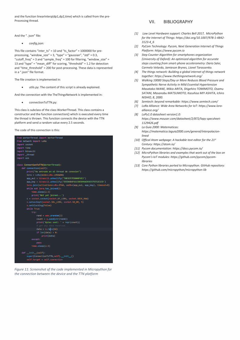
connectionToTTN.py:

This class is subclass of the class WorkerThread. This class contains a constructor and the function connection() which is executed every time the thread is thrown. This function connects the device with the TTN platform and send a random value every 2.5 seconds.

The code of this connection is this:

Figure 11: Screenshot of the code implemented in Micropython for the connection between the device and the TTN platform

VII. BIBLIOGRAPHY

[1] Low Level Hardware support: Charles Bell 2017, MicroPython for the Internet of Things: https://doi.org/10.1007/978-1-4842-3123-4_6

[2] PyCom Technology: Pycom, Next Generation Internet of Things Platform: https://www.pycom.io

[3] Step Counter Algorithm for smartphones organization (University of Oxford): An optimized algorithm for accurate steps counting from smart-phone accelerometry: Dario Salvi, Carmelo Velardo, Jamieson Brynes, Lionel Tarassenko.

[4] The things network: Building a global internet of things network together: https://www.thethingsnetwork.org/

[5] Walking 10000 Steps/Day or More Reduces Blood Pressure and Sympathetic Nerve Activity in Mild Essential Hypertension Masataka IWANE, Mikio ARITA, Shigehiro TOMIMOTO, Osamu SATANI, Masanobu MATSUMOTO, Kazuhisa MIY ASHITA, Ichiro NISHIO, 8, 2000.

[6] Semtech: beyond remarkable: https://www.semtech.com/ [7] LoRa Alliance: Wide Area Networks for IoT: https://www.lora-

alliance.org/ [8] LoPy1.0 datasheet version1.0:

https://www.mouser.com/datasheet/2/872/lopy-specsheet-1129426.pdf

[9] La Guia 2000: Matematicas: https://matematica.laguia2000.com/general/interpolacion-lineal

[10] Offical Atom webpage: A hackable text editor for the 21st Century: https://atom.io/

[11] Pycom documentation: https://docs.pycom.io/ [12] MicroPython libraries and examples that work out of the box on

Pycom’s IoT modules: https://github.com/pycom/pycom-libraries

[13] Core Python libraries ported to Micropython. GitHub repository: https://github.com/micropython/micropython-lib