Texture Mapping for 3D Reconstruction with RGB-D Sensor

Yanping Fu1 Qingan Yan2 Long Yang3 Jie Liao1 Chunxia Xiao1

1 School of Computer, Wuhan University, China2 JD.com

3 College of Information Engineering, Northwest A&F University, China

{ypfu,liaojie,cxxiao}@whu.edu.cn, qingan.yan@jd.com, yl@nwsuaf.edu.cn

Abstract

Acquiring realistic texture details for 3D models is im-

portant in 3D reconstruction. However, the existence of ge-

ometric errors, caused by noisy RGB-D sensor data, always

makes the color images cannot be accurately aligned on-

to reconstructed 3D models. In this paper, we propose a

global-to-local correction strategy to obtain more desired

texture mapping results. Our algorithm first adaptively s-

elects an optimal image for each face of the 3D model,

which can effectively remove blurring and ghost artifacts

produced by multiple image blending. We then adopt a non-

rigid global-to-local correction step to reduce the seaming

effect between textures. This can effectively compensate for

the texture and the geometric misalignment caused by cam-

era pose drift and geometric errors. We evaluate the pro-

posed algorithm in a range of complex scenes and demon-

strate its effective performance in generating seamless high

fidelity textures for 3D models.

1. Introduction

With the emergence of RGB-D sensors, 3D reconstruc-

tion has made significant progress in recent years. While

both small-scale objects and large-scale scenes can be mod-

eled with impressive geometric details [10, 17, 26, 27, 28],

the recovered texture fidelity for 3D models is still less sat-

isfactory [7, 13, 22].

Why does texture mapping technology lag so behind 3D

modeling? The reasons are fourfold: 1) Due to the noise

of depth data, reconstructed 3D models always accompa-

ny geometric errors and distortions. 2) In camera trajectory

estimation, the pose residual would be gradually accumu-

lated and lead to camera drift. 3) The timestamp between

captured depth frame and color frame is not completely syn-

chronized. 4) RGB-D sensors are usually in low resolution,

and the color image is also vulnerable to light and motion

conditions. All of the challenges above contribute to the

produce of misalignments between geometric models and

corresponding images and lead to undesired mapping re-

sults.

While projective mapping methods [21, 23] can re-

duce blurring and ghosting artifacts caused by multi-image

blending, the texture bleeding is unavoidable on the bound-

ary of different views, due to geometric registration errors

and camera trajectory drift. Zhou and Koltun [30] pro-

pose an optimization framework using local image warping,

which can compensate for geometric misalignments. How-

ever, this method needs to subdivide the mesh model, which

will greatly increases the amount of data and limit its appli-

cation scope. Furthermore, the weighted average strategy

which is usually adopted in multi-image blending is sensi-

tive to the light change and motion blur cased by fast camera

movement.

To overcome the challenges, in this paper we propose a

novel texture mapping method which performs a global-to-

local non-rigid correction optimization. First, we choose an

optimal image for each face to avoid the artificial effects

in multi-image blending. In the global optimization step,

we use a unified color consistency and geometry consisten-

cy optimization to rectify the camera pose of each texture

block from different views. Then in the local optimization

step, we find an additional transformation for boundary ver-

tices of the block to refine the texture coordinate drift caused

by geometric errors. Finally, we adopt the texture atlases to

map the texture onto desired 3D model.

We validate the effectiveness of the proposed method in a

range of complex scenes and show high fidelity textures. In

contrast to the method [30], our method is much faster and

needs much less triangle information. The texture blurring

artifacts are also greatly eliminated. As compared to [23],

our method can effectively reduce the seam inconsistency

between face boundaries and is tolerant of geometric mis-

alignments.

2. Related Work

Texture mapping is an important step for acquiring real-

istic 3D models [11, 16, 26, 29]. In this section, we revisit

4645

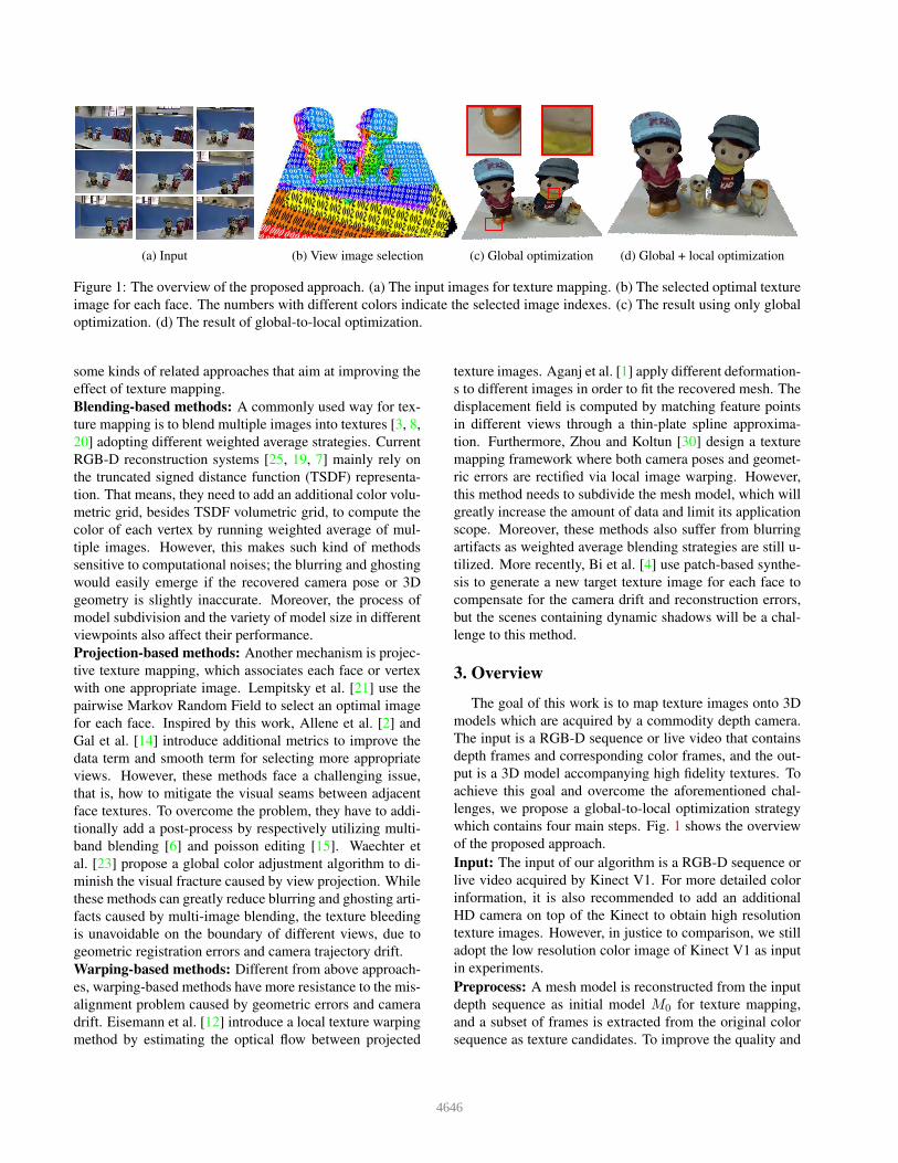
(a) Input (b) View image selection (c) Global optimization (d) Global + local optimization

Figure 1: The overview of the proposed approach. (a) The input images for texture mapping. (b) The selected optimal texture

image for each face. The numbers with different colors indicate the selected image indexes. (c) The result using only global

optimization. (d) The result of global-to-local optimization.

some kinds of related approaches that aim at improving the

effect of texture mapping.

Blending-based methods: A commonly used way for tex-

ture mapping is to blend multiple images into textures [3, 8,

20] adopting different weighted average strategies. Current

RGB-D reconstruction systems [25, 19, 7] mainly rely on

the truncated signed distance function (TSDF) representa-

tion. That means, they need to add an additional color volu-

metric grid, besides TSDF volumetric grid, to compute the

color of each vertex by running weighted average of mul-

tiple images. However, this makes such kind of methods

sensitive to computational noises; the blurring and ghosting

would easily emerge if the recovered camera pose or 3D

geometry is slightly inaccurate. Moreover, the process of

model subdivision and the variety of model size in different

viewpoints also affect their performance.

Projection-based methods: Another mechanism is projec-

tive texture mapping, which associates each face or vertex

with one appropriate image. Lempitsky et al. [21] use the

pairwise Markov Random Field to select an optimal image

for each face. Inspired by this work, Allene et al. [2] and

Gal et al. [14] introduce additional metrics to improve the

data term and smooth term for selecting more appropriate

views. However, these methods face a challenging issue,

that is, how to mitigate the visual seams between adjacent

face textures. To overcome the problem, they have to addi-

tionally add a post-process by respectively utilizing multi-

band blending [6] and poisson editing [15]. Waechter et

al. [23] propose a global color adjustment algorithm to di-

minish the visual fracture caused by view projection. While

these methods can greatly reduce blurring and ghosting arti-

facts caused by multi-image blending, the texture bleeding

is unavoidable on the boundary of different views, due to

geometric registration errors and camera trajectory drift.

Warping-based methods: Different from above approach-

es, warping-based methods have more resistance to the mis-

alignment problem caused by geometric errors and camera

drift. Eisemann et al. [12] introduce a local texture warping

method by estimating the optical flow between projected

texture images. Aganj et al. [1] apply different deformation-

s to different images in order to fit the recovered mesh. The

displacement field is computed by matching feature points

in different views through a thin-plate spline approxima-

tion. Furthermore, Zhou and Koltun [30] design a texture

mapping framework where both camera poses and geomet-

ric errors are rectified via local image warping. However,

this method needs to subdivide the mesh model, which will

greatly increase the amount of data and limit its application

scope. Moreover, these methods also suffer from blurring

artifacts as weighted average blending strategies are still u-

tilized. More recently, Bi et al. [4] use patch-based synthe-

sis to generate a new target texture image for each face to

compensate for the camera drift and reconstruction errors,

but the scenes containing dynamic shadows will be a chal-

lenge to this method.

3. Overview

The goal of this work is to map texture images onto 3D

models which are acquired by a commodity depth camera.

The input is a RGB-D sequence or live video that contains

depth frames and corresponding color frames, and the out-

put is a 3D model accompanying high fidelity textures. To

achieve this goal and overcome the aforementioned chal-

lenges, we propose a global-to-local optimization strategy

which contains four main steps. Fig. 1 shows the overview

of the proposed approach.

Input: The input of our algorithm is a RGB-D sequence or

live video acquired by Kinect V1. For more detailed color

information, it is also recommended to add an additional

HD camera on top of the Kinect to obtain high resolution

texture images. However, in justice to comparison, we still

adopt the low resolution color image of Kinect V1 as input

in experiments.

Preprocess: A mesh model is reconstructed from the input

depth sequence as initial model M0 for texture mapping,

and a subset of frames is extracted from the original color

sequence as texture candidates. To improve the quality and

4646

reduce computation complexity, unlike [30], we utilize [28]

to reconstruct 3D models instead of KinectFusion [18, 22],

and select texture candidate images by weighting the ele-

ments of image clarity, jitter, blur and viewport overlay.

This step produce an initial model M0 and a set of cam-

era poses {T0

i } corresponding to the selected color image

subsequence {Ci} and depth image subsequence {Di}.

Optimization: To construct high fidelity texture, our ap-

proach combines the advantages of [23] and [30]. We select

an optimal texture image for each face of the model to avoid

the blurring caused by multi-image blending. Thus by re-

garding each candidate image as a label, we formulate the

selection problem into a multi-label Markov field in compa-

ny with the angle between camera poses and normal map,

projection area and the distance from model face to camera

plane. However, because both T0 and M0 are not absolutely

accurate, adjacent faces with different labels usually can not

be completely stitched. To solve this problem, we adopt a

global-to-local optimization strategy. For global optimiza-

tion, we adjust the camera pose of each texture block based

on the color consistency and geometric consistency between

relevant blocks. In local optimization stage, we import an

additional transformation to refine texture coordinates on

the boundary of the different blocks and make seamlessly

stitched textures.

Texture Atlases: Finally, we utilize texture atlases to map

the desired texture onto 3D models. Each face is project-

ed onto its associated texture image, under optimized cam-

era pose, to get projection region. Every projected region

is used to establish the texture atlases, while recording the

vertex coordinate of each triangle face. We then transfor-

m them into atlases space. In this way, the texture of each

vertex can be directly retrieved in atlases via texture coordi-

nates, and generate the final textured model.

4. Texture Mapping Method

In this section we will elaborate on each step in more

detail. Let M0 represent the reconstructed mesh model for

texture mapping, {vi} and {fi} are respectively the vertex

set and the face set of M0, where each face represents a

triangle mesh on the model. T is a 4 × 4 transformation

matrix, which transforms the vertex vi of M0 from world

coordinates to local camera coordinates, as defined by:

T =

[

R t

0 1

]

, (1)

where R is the 3×3 rotate matrix and t is the 3×1 translation

vector.

We also specify the perspective projection of a 3D vertex

v = [x, y, z]T onto 2D image plane as Π. Thus the pixel

coordinate u(u, v) for the vertex v on the image plane can

be computed through:

u(u, v)) = Π(Kv) = (x fx

z+ cx ,

yfy

z+ cy)

T , (2)

where K is the camera intrinsic matrix, fx, fy are the focal

lengths, and cx, cy correspond to the coordinate of the cam-

era center in pinhole camera model. Furthermore, we use

D representing depth image, C denoting color image and I

corresponding to the intensity of color image.

4.1. Model Reconstruction

The input of our pipeline is a stream of depth images

and an accompanying RGB color sequence. In our system,

we make use of Microsoft Kinect V1 to capture these data.

As the input frames of Kinect V1 are in low resolution and

would be easily influenced by motion blur and jitter effect,

we thus select a subset of high confidence frames for scene

modeling and texture mapping.

Our method utilize the sparse-sequence fusion (SSF)

method [28], instead of KinectFusion [18, 22], to recon-

struct the initial 3D model and extract high confidence col-

or frames. This method takes account of the jitter, blur and

some other factors that contribute to noises in scanning. It

can reconstruct a mesh model M0 with a sparse depth im-

age sequence {Di}. The basic function of [28] is defined as

follows:

Essf = λ1Ejit(i)+λ2Edif (i)+λ3Evel(i)+Esel(i), (3)

where Esel(i) is a switch term controls the selection of depth

image Di. It should be set to 1 if current image is considered

as valid image to be integrated, otherwise it takes 0. Ejit(i)

measures the jittering effect via calculating the instant view-

point change between selected images. The continuity term

Edif (i) is to ensure sufficient scene overlap between two

selected supporting images by accumulating camera pose

change, and Evel(i) evaluates the camera motion velocity.

Besides of these elements, in order to get high clarity im-

ages, we additionally import a term to depict the quality of

each color frame. Eq. 4 shows our objective function for

frame extraction:

E(i) = Essf (i) + λclaEcla(i), (4)

where Essf is the SSF term and λcla is a balance parameter.

We use λcla = 10 in our experiments, and the others are set

in accordance with [28]. Clarity term Ecla is defined as:

Ecla(i) =

{

expθi − 1, if Esel == 10. if Esel == 0

(5)

The blurriness value θ is calculated via [9]. Eq. 5 shows

that once the depth image Di is added into the supporting

subset, the clarity of its corresponding color image Ci has to

4647

be calculated; otherwise, ignored directly, according to the

value of Esel(i). The iteration proceeds until all captured

images have been processed. This will produce a sparse col-

or image sequence {Ci} with associate camera poses {T0

i },

which can be used as the texture candidates.

4.2. Texture Image Selection

Many texture mapping methods [3, 8, 20] project mesh

onto multiple image planes, and then adopt weighted aver-

age blending strategy to synthesize model textures from pix-

els [11, 16]. They ideally assume that the estimated geom-

etry surfaces and camera poses are enough accurate, how-

ever in practice, this would be easily violated. Therefore,

instead of directly synthesizing from multiple images, we

respectively select an optimal texture image for each face

of the model M0. By regarding each candidate image as a

label, we formulate this selection problem into a pairwise

Markov Random Field (MRF) based on [2]:

E(C) = Ed(C) + λEs(C). (6)

The data term Ed projects each model face onto each

candidate image Ci and measure the area of projection re-

gion, which is related to the angle view proximity, angle,

image resolution, and visibility constraint, as defined by:

Ed(C) = −

{Ci}∑

i

{fj}∑

j

area[ΠCi(fj)]. (7)

The smooth term Es, described by Eq. 8, calculates the

integral along edge e to measures color differences, where

e is the common edge between adjacent faces assigned to

different texture images (Ci,Cj). ε is the entire edge set of

the model M0.

Es(C) =∑

eij∈ε

∫

e

∥

∥ICi(ΠCi

(x))− ICj(ΠCj

(x))∥

∥ dx. (8)

The MRF function E(C) of Eq. 6 is minimized with

graph cuts and alpha expansion [5].

4.3. Global Optimization

The above step associates each face with an texture im-

age Ci. However, due to the existence of geometry error and

camera drift, directly using texture stitching or color adjust-

ment post-processing [21, 14] cannot make the textures on

adjacent faces visually consistent. This is the main chal-

lenge for projective texture mapping methods. To eliminate

visual seams, we draw upon the idea of non-grid correction

to stitch textures between adjacent faces.

Through extrinsic matrix T0 and intrinsic matrix K,

model faces can be easily projected to their associate images

to obtain texture colors. Yet matrix {T0

i } are always noisy,

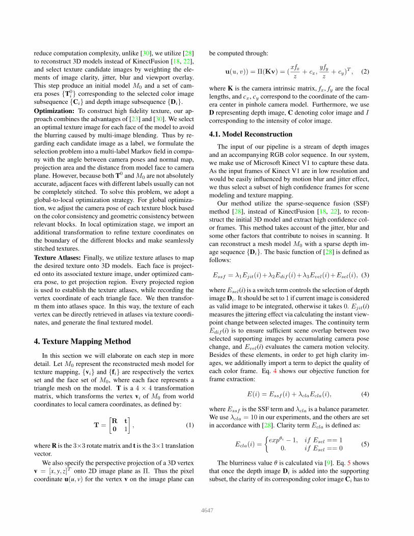
Figure 2: Clustering the model faces according to their tex-

ture images.

so that the texture colors obtained through these transforma-

tions may be also inaccurate. In this section, we thus have to

optimize {T0

i } to make sure that all the faces coming from

different texture images can be closely aligned.

We first perform a face clustering process based on tex-

ture image {Ci}, that is, if two adjacent faces correspond to

the same texture image, we put them together in the same

labeled cluster. After traversing all faces, a collection of

clusters can be obtained, as shown in Fig. 2 with different

colors. For the sake of clarity, we name that the all faces

within the same cluster as a chart. In order to improve ro-

bustness, if the number of faces Fi in a chart i is less than

a threshold FN , this chart will be merged into its closest

neighbor j, which is measured by three elements: 1) The

viewpoint angle between texture images of chart i and j

should be minimal. 2) The number of faces meets the crite-

ria of Fj > FN . 3) The projection of all vertices in chart i

onto the texture image of chart j should still stay in bound-

s. We empirically set FN = 50 in our subsequent exper-

iments. Based on the clusters, we establish an undirected

connection graph G from the charts; if two charts are ad-

jacent to each other, there will be an edge gij ∈ G linking

them.

The texture for faces in the chart comes from the same

image, so they are well aligned. That means, in order to

generate a natural texture for the model, we only need to

adjust the textures between different charts. For ideal tex-

ture mapping, we believe that the boundary texture of one

chart can be totally recovered by the texture of its adjacen-

t charts. Based on this observation, we can align adjacent

chart textures as long as it is possible to minimize the incon-

sistency between associated texture and projected texture of

each chart and its neighbors. However, only considering the

color consistency may lead to misalignment in texture-less

regions. Therefore, we additionally take the geometric con-

sistency into consideration, which serves as a regular term

in Eq. 9. We formulate our objective function as follows by

4648

measuring both color consistency and geometric consisten-

cy for each chart:

E(T) =

chartN∑

i

∑

j∈Gi

N∑

k∈charti

(Ii(Π(Tivk)− Ij(Π(Tjvk)))2

+ λdepth

chartN∑

i

N∑

k∈charti

(ϕ(Tivk)−Di(Π(Tivk)))2

,

(9)

where vk denotes the whole vertex set in chart i and N is its

number. chartN represents the number of chart on model

M0. Function ϕ(x) computes the Z component of the vec-

tor x. Gi depicts the neighborhood of chart i. The first term

makes the texture of chart i consistent with the projected

texture of its adjacent chart j. The second term ensure that,

when T changes, the optimized camera pose not only makes

the texture consistent, but also the reconstructed model to be

consistent with the depth image acquired by RGB-D camer-

a, and ensure the camera pose T not to deviate far apart from

the initial value T0 when the color constraint is insufficien-

t. By minimizing the Eq. 9, we can compute a correction

transformation matrix for each chart, which makes the ad-

jacent charts closer to each other and reduces visual seams.

4.4. Local Optimization

While the global optimization is able to make most tex-

tural regions stitched, for some areas with large geometric

errors (as shown in the red box of Fig. 1(c)), the textures

still could not be accurately aligned. The global optimiza-

tion can only correct the camera drift of each chart. If the

reconstructed geometric model is accurate enough, all tex-

tures will be well stitched after the global optimization. Un-

fortunately, the ubiquity of geometry errors makes the only

global optimization is insufficient for high fidelity texture

mapping. Thus we introduce a further adjustment on each

face of the model so that local textures can be also well

aligned.

Because all faces on one chart correspond to the same

texture image, there is therefore no need to optimize the

entire chart. In addition, as each chart has been roughly

aligned in the global optimization step, it is only necessary

to perform correcting on a small set of vertices to make up

for texture misalignment caused by geometric errors. In-

stead of editing the mesh model, we propose to warp the

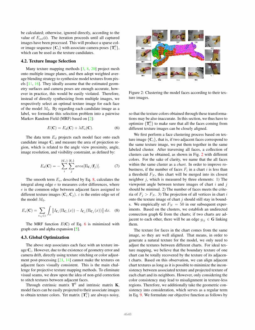
projected coordinates of boundary vertices in each chart. As

shown in Fig. 3(b), in order to align the texture at vertex v,

we can move the projected coordinate of v in image A to

align the texture of v in image B. As long as the bound-

ary vertices are optimized, the texture of whole chart will

be well aligned.

However, moving the projection coordinate of a vertex

is a ill-posed problem. To address the challenge, we find

(a)

(b)

Figure 3: (a) The projection area of two adjacent charts onto

their respective texture images. (b) Correcting the texture

coordinate of the vertex v in chart A makes it align to the

coordinate of vertex v in the texture image of chart B.

an optimal moving vector for the texture coordinate of each

boundary vertex and make it aligned with its adjacent chart

textures. To this end, we compute an additional transforma-

tion matrix for the vertex v on the boundary of chart instead

of calculating the moving vector directly. The additional

transformation ensures that the chart where the vertex v is

located is sufficiently aligned with the charts connected to

v. Then we use this matrix to obtain the optimal projection

coordinate for v as texture coordinate. The texture coordi-

nate correction process is able to make the local texture at

each boundary vertex v to be sufficiently aligned. We de-

sign an objective function to compute this matrix of v to

correct texture coordinate in the image as follows:

E(Tij)=

chartN∑

i

vertN∑

j

adjN∑

k

(Ii(Π(TijTivj)))

−Ik(Π(TkjTkvj)))2 + λreg

chartN∑

i

vertN∑

j

(TTijTij − I)

,

(10)

where j represents the boundary vertex of chart i, k rep-

resents the adjacent charts of i which share vertex j and v

represents the whole vertices in chart i. Tij is an additional

4649

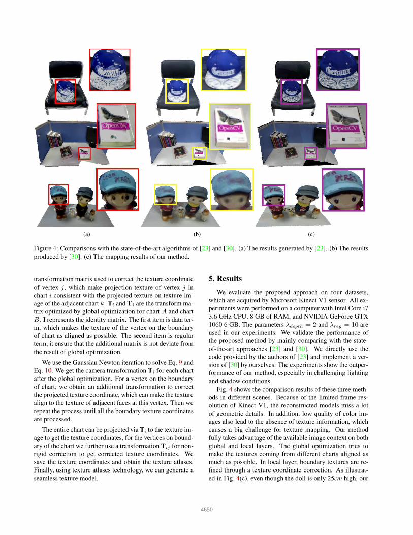
(a) (b) (c)

Figure 4: Comparisons with the state-of-the-art algorithms of [23] and [30]. (a) The results generated by [23]. (b) The results

produced by [30]. (c) The mapping results of our method.

transformation matrix used to correct the texture coordinate

of vertex j, which make projection texture of vertex j in

chart i consistent with the projected texture on texture im-

age of the adjacent chart k. Ti and Tj are the transform ma-

trix optimized by global optimization for chart A and chart

B. I represents the identity matrix. The first item is data ter-

m, which makes the texture of the vertex on the boundary

of chart as aligned as possible. The second item is regular

term, it ensure that the additional matrix is not deviate from

the result of global optimization.

We use the Gaussian Newton iteration to solve Eq. 9 and

Eq. 10. We get the camera transformation Ti for each chart

after the global optimization. For a vertex on the boundary

of chart, we obtain an additional transformation to correct

the projected texture coordinate, which can make the texture

align to the texture of adjacent faces at this vertex. Then we

repeat the process until all the boundary texture coordinates

are processed.

The entire chart can be projected via Ti to the texture im-

age to get the texture coordinates, for the vertices on bound-

ary of the chart we further use a transformation Tij for non-

rigid correction to get corrected texture coordinates. We

save the texture coordinates and obtain the texture atlases.

Finally, using texture atlases technology, we can generate a

seamless texture model.

5. Results

We evaluate the proposed approach on four datasets,

which are acquired by Microsoft Kinect V1 sensor. All ex-

periments were performed on a computer with Intel Core i7

3.6 GHz CPU, 8 GB of RAM, and NVIDIA GeForce GTX

1060 6 GB. The parameters λdepth = 2 and λreg = 10 are

used in our experiments. We validate the performance of

the proposed method by mainly comparing with the state-

of-the-art approaches [23] and [30]. We directly use the

code provided by the authors of [23] and implement a ver-

sion of [30] by ourselves. The experiments show the outper-

formance of our method, especially in challenging lighting

and shadow conditions.

Fig. 4 shows the comparison results of these three meth-

ods in different scenes. Because of the limited frame res-

olution of Kinect V1, the reconstructed models miss a lot

of geometric details. In addition, low quality of color im-

ages also lead to the absence of texture information, which

causes a big challenge for texture mapping. Our method

fully takes advantage of the available image context on both

global and local layers. The global optimization tries to

make the textures coming from different charts aligned as

much as possible. In local layer, boundary textures are re-

fined through a texture coordinate correction. As illustrat-

ed in Fig. 4(c), even though the doll is only 25cm high, our

4650

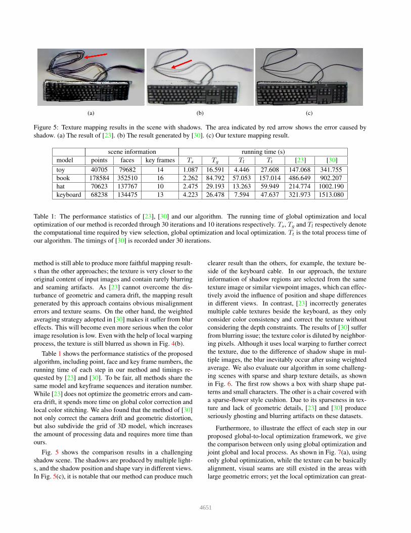
(a) (b) (c)

Figure 5: Texture mapping results in the scene with shadows. The area indicated by red arrow shows the error caused by

shadow. (a) The result of [23]. (b) The result generated by [30]. (c) Our texture mapping result.

scene information running time (s)

model points faces key frames Ts Tg Tl Tt [23] [30]

toy 40705 79682 14 1.087 16.591 4.446 27.608 147.068 341.755

book 178584 352510 16 2.262 84.792 57.053 157.014 486.649 902.207

hat 70623 137767 10 2.475 29.193 13.263 59.949 214.774 1002.190

keyboard 68238 134475 13 4.223 26.478 7.594 47.637 321.973 1513.080

Table 1: The performance statistics of [23], [30] and our algorithm. The running time of global optimization and local

optimization of our method is recorded through 30 iterations and 10 iterations respectively. Ts, Tg and Tl respectively denote

the computational time required by view selection, global optimization and local optimization. Tt is the total process time of

our algorithm. The timings of [30] is recorded under 30 iterations.

method is still able to produce more faithful mapping result-

s than the other approaches; the texture is very closer to the

original content of input images and contain rarely blurring

and seaming artifacts. As [23] cannot overcome the dis-

turbance of geometric and camera drift, the mapping result

generated by this approach contains obvious misalignment

errors and texture seams. On the other hand, the weighted

averaging strategy adopted in [30] makes it suffer from blur

effects. This will become even more serious when the color

image resolution is low. Even with the help of local warping

process, the texture is still blurred as shown in Fig. 4(b).

Table 1 shows the performance statistics of the proposed

algorithm, including point, face and key frame numbers, the

running time of each step in our method and timings re-

quested by [23] and [30]. To be fair, all methods share the

same model and keyframe sequences and iteration number.

While [23] does not optimize the geometric errors and cam-

era drift, it spends more time on global color correction and

local color stitching. We also found that the method of [30]

not only correct the camera drift and geometric distortion,

but also subdivide the grid of 3D model, which increases

the amount of processing data and requires more time than

ours.

Fig. 5 shows the comparison results in a challenging

shadow scene. The shadows are produced by multiple light-

s, and the shadow position and shape vary in different views.

In Fig. 5(c), it is notable that our method can produce much

clearer result than the others, for example, the texture be-

side of the keyboard cable. In our approach, the texture

information of shadow regions are selected from the same

texture image or similar viewpoint images, which can effec-

tively avoid the influence of position and shape differences

in different views. In contrast, [23] incorrectly generates

multiple cable textures beside the keyboard, as they only

consider color consistency and correct the texture without

considering the depth constraints. The results of [30] suffer

from blurring issue; the texture color is diluted by neighbor-

ing pixels. Although it uses local warping to further correct

the texture, due to the difference of shadow shape in mul-

tiple images, the blur inevitably occur after using weighted

average. We also evaluate our algorithm in some challeng-

ing scenes with sparse and sharp texture details, as shown

in Fig. 6. The first row shows a box with sharp shape pat-

terns and small characters. The other is a chair covered with

a sparse-flower style cushion. Due to its sparseness in tex-

ture and lack of geometric details, [23] and [30] produce

seriously ghosting and blurring artifacts on these datasets.

Furthermore, to illustrate the effect of each step in our

proposed global-to-local optimization framework, we give

the comparison between only using global optimization and

joint global and local process. As shown in Fig. 7(a), using

only global optimization, while the texture can be basically

alignment, visual seams are still existed in the areas with

large geometric errors; yet the local optimization can great-

4651

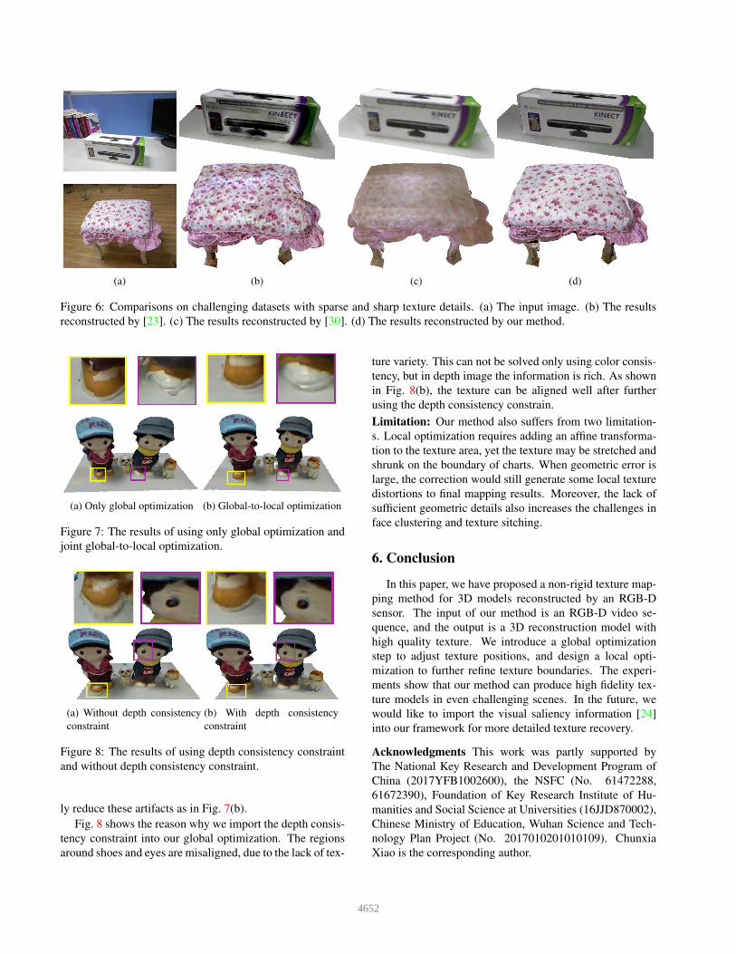
(a) (b) (c) (d)

Figure 6: Comparisons on challenging datasets with sparse and sharp texture details. (a) The input image. (b) The results

reconstructed by [23]. (c) The results reconstructed by [30]. (d) The results reconstructed by our method.

(a) Only global optimization (b) Global-to-local optimization

Figure 7: The results of using only global optimization and

joint global-to-local optimization.

(a) Without depth consistency

constraint

(b) With depth consistency

constraint

Figure 8: The results of using depth consistency constraint

and without depth consistency constraint.

ly reduce these artifacts as in Fig. 7(b).

Fig. 8 shows the reason why we import the depth consis-

tency constraint into our global optimization. The regions

around shoes and eyes are misaligned, due to the lack of tex-

ture variety. This can not be solved only using color consis-

tency, but in depth image the information is rich. As shown

in Fig. 8(b), the texture can be aligned well after further

using the depth consistency constrain.

Limitation: Our method also suffers from two limitation-

s. Local optimization requires adding an affine transforma-

tion to the texture area, yet the texture may be stretched and

shrunk on the boundary of charts. When geometric error is

large, the correction would still generate some local texture

distortions to final mapping results. Moreover, the lack of

sufficient geometric details also increases the challenges in

face clustering and texture sitching.

6. Conclusion

In this paper, we have proposed a non-rigid texture map-

ping method for 3D models reconstructed by an RGB-D

sensor. The input of our method is an RGB-D video se-

quence, and the output is a 3D reconstruction model with

high quality texture. We introduce a global optimization

step to adjust texture positions, and design a local opti-

mization to further refine texture boundaries. The experi-

ments show that our method can produce high fidelity tex-

ture models in even challenging scenes. In the future, we

would like to import the visual saliency information [24]

into our framework for more detailed texture recovery.

Acknowledgments This work was partly supported by

The National Key Research and Development Program of

China (2017YFB1002600), the NSFC (No. 61472288,

61672390), Foundation of Key Research Institute of Hu-

manities and Social Science at Universities (16JJD870002),

Chinese Ministry of Education, Wuhan Science and Tech-

nology Plan Project (No. 2017010201010109). Chunxia

Xiao is the corresponding author.

4652

References

[1] E. Aganj, P. Monasse, and R. Keriven. Multi-view texturing

of imprecise mesh. In Asian Conference on Computer Vision,

pages 468–476, 2009.

[2] C. Allene, J. P. Pons, and R. Keriven. Seamless image-based

texture atlases using multi-band blending. In International

Conference on Pattern Recognition, pages 1–4, 2008.

[3] F. Bernardini, I. M. Martin, and H. Rushmeier. High-quality

texture reconstruction from multiple scans. Visualization &

Computer Graphics IEEE Transactions on, 7(4):318–332,

2001.

[4] S. Bi, N. K. Kalantari, and R. Ramamoorthi. Patch-based

optimization for image-based texture mapping. ACM Trans-

actions on Graphics, 36(4), 2017.

[5] Y. Boykov, O. Veksler, and R. Zabih. Fast approximate ener-

gy minimization via graph cuts. IEEE Transactions on Pat-

tern Analysis and Machine Intelligence, 23:2001, 2001.

[6] P. J. Burt and E. H. Adelson. A multiresolution spline

with application to image mosaics. ACM Trans. Graph.,

2(4):217–236, 1983.

[7] E. Bylow, J. Sturm, C. Kerl, F. Kahl, and D. Cremers. Real-

time camera tracking and 3d reconstruction using signed dis-

tance functions. In Robotics: Science and Systems, 2013.

[8] M. Callieri, P. Cignoni, M. Corsini, and R. Scopigno.

Masked photo blending: Mapping dense photographic da-

ta set on high-resolution sampled 3d models. Computers &

Graphics, 32(4):464–473, 2008.

[9] F. Crete, T. Dolmiere, P. Ladret, and M. Nicolas. The blur

effect: perception and estimation with a new no-reference

perceptual blur metric. In Electronic Imaging, pages 64920I–

64920I–11, 2007.

[10] A. Dai, S. Izadi, and C. Theobalt. Bundlefusion: real-time

globally consistent 3d reconstruction using on-the-fly surface

re-integration. Acm Transactions on Graphics, 36(4):76a,

2017.

[11] L. Do, L. Ma, E. Bondarev, and P. H. N. D. With. On multi-

view texture mapping of indoor environments using kinect

depth sensors. In International Conference on Computer Vi-

sion Theory and Applications, pages 739–745, 2015.

[12] M. Eisemann, B. D. Decker, M. Magnor, P. Bekaert, E. D.

Aguiar, N. Ahmed, C. Theobalt, and A. Sellent. Floating

textures. Computer Graphics Forum, 27(2):409C418, 2008.

[13] N. Fioraio, J. Taylor, A. Fitzgibbon, and L. D. Stefano.

Large-scale and drift-free surface reconstruction using on-

line subvolume registration. In CVPR, 2015.

[14] R. Gal, Y. Wexler, E. Ofek, H. Hoppe, and D. Cohen-Or.

Seamless montage for texturing models. Eurographics 2010,

29/2, May 2010.

[15] M. Gangnet and A. Blake. Poisson image editing. In ACM

SIGGRAPH, pages 313–318, 2003.

[16] L. Grammatikopoulos, I. Kalisperakis, G. Karras, and E. Pet-

sa. Automatic multi-view texture mapping of 3d surface pro-

jections. pages 12–13, 2007.

[17] M. Halber and T. Funkhouser. Fine-to-coarse global regis-

tration of rgb-d scans. In CVPR, 2017.

[18] S. Izadi, D. Kim, O. Hilliges, D. Molyneaux, R. Newcombe,

P. Kohli, J. Shotton, S. Hodges, D. Freeman, and A. Davison.

Kinectfusion:real-time 3d reconstruction and interaction us-

ing a moving depth camera. In ACM Symposium on User

Interface Software and Technology, Santa Barbara, Ca, Usa,

October, pages 559–568, 2011.

[19] S. Izadi and M. Stamminger. Real-time 3d reconstruction at

scale using voxel hashing. Acm Transactions on Graphics,

32(6):169, 2013.

[20] W. Kehl, N. Navab, and S. Ilic. Coloured signed distance

fields for full 3d object reconstruction. In Proceedings of the

British Machine Vision Conference. BMVA Press, 2014.

[21] V. Lempitsky and D. Ivanov. Seamless mosaicing of image-

based texture maps. In CVPR, pages 1–6, 2007.

[22] R. A. Newcombe, S. Izadi, O. Hilliges, D. Molyneaux,

D. Kim, A. J. Davison, P. Kohi, J. Shotton, S. Hodges, and

A. Fitzgibbon. Kinectfusion: Real-time dense surface map-

ping and tracking. In IEEE International Symposium on

Mixed and Augmented Reality, pages 127–136, 2011.

[23] M. Waechter, N. Moehrle, and M. Goesele. Let there be col-

or! large-scale texturing of 3d reconstructions. In European

Conference on Computer Vision, pages 836–850, 2014.

[24] W. Wang, J. Shen, and L. Shao. Consistent video saliency

using local gradient flow optimization and global refinement.

IEEE Transactions on Image Processing, 24(11):4185–4196,

2015.

[25] T. Whelan, M. Kaess, H. Johannsson, M. Fallon, J. J.

Leonard, and J. Mcdonald. Real-time large-scale dense rgb-

d slam with volumetric fusion. International Journal of

Robotics Research, 34(4-5):598–626, 2015.

[26] T. Whelan, S. Leutenegger, R. S. Moreno, B. Glocker, and

A. Davison. Elasticfusion: Dense slam without a pose graph.

In Robotics: Science and Systems, 2015.

[27] Q. Yan, L. Yang, L. Zhang, and C. Xiao. Distinguishing

the indistinguishable: Exploring structural ambiguities via

geodesic context. In CVPR, pages 3836–3844, 2017.

[28] L. Yang, Q. Yan, Y. Fu, and C. Xiao. Surface reconstruction

via fusing sparse-sequence of depth images. IEEE Transac-

tions on Visualization and Computer Graphics, 2017.

[29] L. Yang, Q. Yan, and C. Xiao. Shape-controllable geometry

completion for point cloud models. The Visual Computer,

33(3):385–398, 2017.

[30] Q. Y. Zhou and V. Koltun. Color map optimization for 3d

reconstruction with consumer depth cameras. Acm Transac-

tions on Graphics, 33(4):1–10, 2014.

4653