TEXTO PARA DISCUSSÃO N°°°° 361

THE SPATIAL STRUCTURE OF THE FINANCIAL DEVELOPMENT IN BRAZIL

Marco Crocco

Fabiana Santos

Pedro Amaral

Setembro de 2009

2

Ficha catalográfica

332.0981

C938s

2009

Crocco, Marco.

The spatial structure of the financial development in

Brazil / Marco Crocco; Fabiana Santos; Pedro Amaral. -

Belo Horizonte: UFMG/Cedeplar, 2009.

30p. (Texto para discussão ; 361)

1. Finanças – Brasil. 2. Mercado financeiro – Brasil.

3. Bancos – Brasil. 4. Desenvolvimento econômico. 5.

Economia regional. I. Santos, Fabiana. II. Amaral,

Pedro. III. Universidade Federal de Minas Gerais.

Centro de Desenvolvimento e Planejamento Regional.

IV. Título. V. Série.

CDD

3

UNIVERSIDADE FEDERAL DE MINAS GERAIS

FACULDADE DE CIÊNCIAS ECONÔMICAS

CENTRO DE DESENVOLVIMENTO E PLANEJAMENTO REGIONAL

THE SPATIAL STRUCTURE OF THE FINANCIAL DEVELOPMENT IN BRAZIL

Marco Crocco Cedeplar/UFMG – crocco@cedeplar.ufmg.br

Fabiana Santos Cedeplar/UFMG – fabiana@cedeplar.ufmg.br

Pedro Amaral Cedeplar/UFMG – pedrovma@cedeplar.ufmg.br

CEDEPLAR/FACE/UFMG

BELO HORIZONTE

2009

4

SUMÁRIO

INTRODUCTION................................................................................................................................... 6

I. FINANCIAL DEVELOPMENT AND THE CENTRAL-PLACE THEORY..................................... 6

I.1. Regional Aspects of the Financial System ................................................................................... 6

I.2. The Central-Place Theory and the Financial System Spatial Structure ...................................... 10

I.3. Liquidity Preference and Centrality............................................................................................ 11

II. ESTIMATION STRATEGY ............................................................................................................ 12

III. EXPLORATORY ANALYSIS....................................................................................................... 16

IV. ESTIMATIVE AND INFERENCE ................................................................................................ 25

FINAL REMARKS............................................................................................................................... 27

REFERENCES...................................................................................................................................... 28

5

RESUMO

Este trabalho analisa a distribuição e transbordamentos espaciais do desenvolvimento do

sistema financeiro à luz da Teoria do Lugar Central e do conceito pós-keynesiano de preferência pela

liquidez regional. Os dados de operações de crédito e imposto sobre operações financeiras (IOF)

utilizados foram extraídos dos balanços consolidados dos municípios brasileiros de 1995 a 2007

fornecidos pelo Banco Central do Brasil. Para investigar a estrutura espacial do sistema financeiro no

Brasil foram utilizados métodos GM para a estimação de um painel espacial com defasagem espacial e

erros de média móvel. Os resultados sugerem uma associação espacial negativa do sistema financeiro

dos municípios brasileiros, de modo que um município com sistema mais desenvolvido em geral se

encontre inserido em meio a sistemas financeiros menos desenvolvidos.

Palavras-chave: desenvolvimento financeiro, estrutura espacial, estratégia bancária, Brasil.

Classificação JEL: O16, R12, G21

ABSTRACT

This paper explores the financial development in Brazil. It focuses on the impacts of the

development level of a municipality’s financial system over its neighborhood, under the light of the

Central Place Theory. Using a GMM estimator for a spatial panel model with an endogenous spatial

lag and spatial moving average errors we investigate the spatial structure of the financial system in

Brazil. The results point to a negative spatial association between the Brazilian municipalities’

financial system, in the way that a municipality with more developed financial system tends to be

surrounded by municipalities with less developed financial systems.

Keywords: financial development, spatial structure, bank strategy, Brazil.

JEL Classification: O16, R12, G21

6

INTRODUCTION

Studies on regional issues in Brazil have focused on the behaviour of the economy’s real

variables (production, employment, wages, etc.), whilst monetary variables have been overlooked. The

paper aims to investigate the spatial distribution of the financial system by exploring the impacts of the

development level of a municipality’s financial system over its neighborhood.

Based on the Post Keynesian concept of regional liquidity preference (Dow, 1993) and the

Central Place Theory (Christäller, 1966), the paper analyses tax on financial operations and credit

operations drawn from consolidated balance sheets of bank branches spread across Brazilian

municipalities in order to verify the spatial structure of the financial system in Brazil.

It is argued that there is substantial evidence that the Brazilian Bank System operates

differentiated strategies across space. Specifically, the results point to a negative spatial association

between the Brazilian municipalities’ financial system, in the way that a municipality with more

developed financial system tends to be surrounded by municipalities with less developed financial

systems.

Our model uses a GMM estimator for a spatial panel model with an endogenous spatial lag

and spatial moving average errors to investigate the spatial structure of the financial system in Brazil.

The yearly municipal data on financial assets for 1995-2007 is from a database compiled by the

Laboratory of Studies in Money and Space (LEMTe) of CEDEPLAR/UFMG from data provided by

the Brazilian Central Bank. The social variables are extracted from the Annual Relation of Social

Variables (RAIS), a Brazilian census of formal firms and its employees.

Apart from this brief introduction, the paper is organized in the following way. The next

section (I), lays out the main theoretical contributions to the understanding of the financial systems’

regional dynamics. In Section II, the estimation strategy is presented. It allows us to estimate not only

the relation between the financial system at one locality and its own attributes, but also the relation

with the financial system at the neighborhood, taking into account omitted variables assumed time-

invariant and its spatial interaction in a moving average process. In Section III, the exploratory

analysis of the evolution of the Brazilian financial system and its regional dynamics is carried out,

considering the evolution of selected variables and indicators and the spatial distribution of the

financial system in 2006. Section IV shows the results of the estimations over the dependent variables

IOF and Credit. In the last section, some conclusions are drawn.

I. FINANCIAL DEVELOPMENT AND THE CENTRAL-PLACE THEORY

I.1. Regional Aspects of the Financial System

The theoretical discussion about regional aspects of the financial system has received different

treatments from regional economists, economic geographers and experts in financial development.

Generally speaking, in the literature of regional economics little attention is given to money and

financial systems and their role in regional development. Most of them assume that the financial

system is neutral in relation to its influence on regional performance.

7

The mainstream literature on financial development, by contrast, has focus for the last 30

years or so on the so-called ‘finance – growth nexus’. The emphasis is placed on the correlation

between financial variables (and the degree of development of the financial system) and economic

growth. Most mainstream economists state that the direction of causality runs from the former to the

latter, although unambiguous evidence is hard to bring about. In this literature, the issue of regional

aspects of the financial system development has been virtually neglected. Indeed, in an extensive

review of the main contributions in this research area, made by Levine (2004), the word “regional”

appears only once on the 118 pages of the review; the word “regions”, twice and the word

“geography”, none. There is only one paper reviewed by Levine that focuses on regions inside a

specific country. This paper - written by Guiso et al. (2002) - shows that local financial conditions

influence economic performance across different regions in Italy. The most important conclusion of

the authors was that national (and regional) financial systems have an important role to play despite

the advance of international financial integration.

Nevertheless, our review of the literature has shown that in fact there has been over the years

important contributions to show the non-neutrality of money and financial systems in terms of their

effects on the real side of the economy, and, therefore, in regional development, as can be found in the

new-Keynesian1 and post-Keynesian theories of financial system.

Overall, the main areas of research of the New-Keynesians have been related to the

investigation of:

i. whether or not regional financial markets exist (Amos and Wingender, 1993; Bias, 1992);

ii. how market failures – i.e. asymmetric information and scale-sensitive transaction and information

costs - affect the efficiency of the financial system in the allocation of credit - and hence the

performance of real variables - among regions of a country (Koo and Moon, 2004, Miyakoshi and

Tsukuda, 2004);

iii. whether or not the distribution of different types of banks across regions of a country (or local

banking systems) explains disparities in regional economic growth (Usai and Vannini, 2005;

Ozyildirim and Older, 2008; Valverde and Fernández, 2004);

iv. whether or not local/regional economic conditions have an impact on local/regional banks’

performance (Meyer and Yeager, 2001; Yeager, 2004; Emmons et al., 2004; Furlong and Kreiner,

2007; Daly et al., 2008);

v. how geographic diversification affects banks’ performance (Demsetz and Strahan, 1997; Acharya

et al., 2002; Morgan and Samolyk, 2005);

vi. how distance between branches and headquarters or between lenders and borrowers influences

credit allocation and availability (Alessandrini and Zazzaro, 1999; Berger and DeYoung, 2001;

Carling and Lundenberg, 2005; Brevoot and Hannan, 2006; Alessandrini et al., 2007).

1 Roberts and Fishkind (1979), Moore and Hill (1982) are authors who first attempted to identify factors that could lead to

credit rationing in regional markets. Recently, neo-Keynesian authors, as Faini et al. (1993) and Samolyk (1994), have

explored the argument of asymmetric information in regional credit markets.

8

As the latter line of enquiry bears directly on the subject of this paper, we will discuss it in

more detail here. The analysis of the relationship between distance and credit allocation/availability

has followed distinct perspectives. A first line of work analyses the distance between banks’

headquarters and branches. Berger and DeYoung (2001) pointed out that inefficiencies tend to

increase with the distance between a bank’s headquarter and its subsidiaries “presumably because the

managers at a faraway subsidiary have more leeway for mismanagement or shirking”. Carling and

Lundenberg (2005) explored whether or the proximity between borrowers and lenders influences the

degree of asymmetric information and thus affects credit availability. They found no evidence that

asymmetric information increases with distance, leading them to conclude that the locational strategy

of banks should be based on factors other than credit risk management. Alessandrini et. al. (2007)

investigated how the distance between bank’s branches and headquarters influences the likelihood of

introducing innovations and credit rationing. They forged the concept of “functional distance”2 to

capture the differences among the functions carried out by headquarters and branches. Their results

showed that bank branches of higher functional distance are less likely to introduce innovations and

are more likely to be credit rationed. Alessandrini et. al. (2008), in turn, examine the impact of

operational and functional distance3 on the financial constraints of Italian firms. They found out that

although greater functional distance has negative impacts over credit availability, especially for small

firms, lower operational distance do not necessarily improve this availability.

A second line of work explores the effects of distance between borrowers and lenders. A first

perspective enquires into screening and monitoring aspects related to the distance between borrowers

and lenders. In this case, distance would work to increase the difficulty of collecting and processing

soft information about borrowers and this would make the process of screening and monitoring loans

more costly. Brevoot and Hannan (2006) investigated the relationship between lending and distance,

especially commercial lending. Their findings suggested that distance between borrowers and lenders

works as restriction to lending. A second perspective delves into the travel costs incurred by a

borrower to meet a lender, as found in Park and Pennacchi (2009). It is worthwhile noticing that this is

what Alessandrini et al. (2008) later termed as “operational distance”.

Now, the post-Keynesian researchers have also made significant contributions to the analysis

of the regional aspects of financial systems. Their analyses differ from the others discussed previously

as they approach both the supply side and the demand side in the regional credit market. According to

this view, the supply of and demand for credit are interdependent and affected by the liquidity

preference, linked to the expectations of economic agents in an uncertain environment.4 From the

viewpoint of the banking system, a high liquidity preference will negatively affect its disposition to

lend money in the region, as it shows pessimistic or less reliable expectations of its economic

2 The term “functional distance” means the distance between hierarchical levels of a bank organization. According to

Alessandrini et al. 2008 (p. 5), “by functional distance we refer to the distance between a local branch, where information is

collected and lending relationships are established, and its headquarter, where lending policies and ultimate decisions are

typically taken. From a theoretical point of view, the importance of functional distance for the lending policies of local

branches has its roots in (i) the asymmetric distribution of information and the costs of communication within an

organisation, and (ii) the economic, social and cultural differences across communities.”

3 Operational distance refers to the proximity between the borrower and its lending office.

4 For a further understanding of the use of such a concept in Keynesian economics, see Davidson (1982/1983, 1995), Dow

(1995) and Crocco (1999, 2003).

9

performance. On the demand side for credit, the liquidity preference of the public or the firms will

affect its respective portfolio decisions. The greater the liquidity preference, the greater is the demand

for net assets and the lesser the demand for credit.

Dow (1982) has added up to the concept of liquidity preference the contributions of Myrdal

(1957) on cumulative causation and the dependence theory to show how their simultaneous operation

can lead to unequal regional development patterns. According to her, the liquidity preference of

residents (banks, entrepreneurs and the public) of less developed regions will be greater than that of

more developed regions. This is related to the specific features of each of these regions, which in turn,

influence the liquidity preference of their residents. The less developed regions are extremely

dependent on the centre for the provision of sophisticated goods and services as their income level and

shallow productive structure are usually insufficient to sustain a dynamic modern economic system5.

Moreover, some institutions are still to be built or (at least) strengthened, markets are feeble and

financial institutions unsophisticated. These regions are also subject to significant economic volatility

and (new) investment opportunities are limited. Consequently, banks would face a higher default risk

of loans and of capital loss and hence charge higher interest rates. Firms, in turn, would experience a

change in the marginal efficiency of investment ad it is affected by the smaller availability of loans

and higher bank interest rates. The public would face considerable uncertainty regarding their

earnings, given the volatility of the local economy and its low level of diversification and

sophistication. Through the mechanism of cumulative causation, such weaknesses of the peripheral

regions would be reinforced over time, while the central regions would grow more diversified and

sophisticated. The peripheral region would experience a “funding gap” and the financial system would

become heavily spatially-centralized in the centre. First, the national banks would lend less money to

peripheral regions, due to their economic structure and the remote control over the branches located in

them. Secondly, local banks of peripheral regions, in turn, would behave defensively by maintaining

high reserve level and restraining local loans. Thirdly, the higher liquidity preference of the public

resident in the peripheral region would be translated into a higher proportion of demand deposits than

of time deposits, which would force banks to curtail their loans terms in order to adjust them to the

smaller portion of time deposits. Four, higher demand for centre securities and thick central financial

markets would encourage the concentration of capital (or loan) markets as well as the agglomeration

of financial activities, institutions and functions in the centre. This, in turn, would work against the

capacity of the peripheral regions to attract bank branches (let alone bank headquarters). At the

economy level, these interdependent and mutually reinforcing processes, left to their own course,

would increase regional disparities, turn the space more fragmented or fractured and the financial

system spatially-centralized into a core-periphery structure (Chick and Dow 1988; Dow 1996, 1999).

In a similar vein, Martin (1999) and Klagge and Martin (2005) bring theoretical and empirical

evidence on the spatial bias on the allocation of funds between peripheral and central regions, which

would contribute to uneven regional development. They advocate the non-neutrality of the relationship

between the financial and the real side of the economic apparatus. According to them financial

systems do not function in a “space-neutral way”.

5 This also means, as noticed by Klagge and Martin (2005), that the peripheral reserve base “is diminished as funds leak out

in payment for centre goods and securities”.

10

That is to say, financial markets across regions within a country would not be perfectly

integrated, so that investment in any given region is dependent of local savings and local demand for

finance is constrained by local supply and residents (the firms and the public) cannot access funds

from anywhere in the national system. Thus, the geographical proximity to the financial centre does

matters. The result is the occurrence of concentration of the financial institutions and functions in

central locations and of sectoral, spatial-funding gaps between the core and the periphery.

Martin (1999) brings to the discussion the importance of “central places” and “centralitality”,

as found in Christaller (1933)6. According to him, as centrality helps to concentrate people and

increases the income of the region, it is possible to argue that the higher the centrality the higher will

be the possibility of a bank deciding to locate a branch in this region.

Let us now turn to the analysis of the relationship between the centrality of a region (city) and

the financial system spatial structure.

I.2. The Central-Place Theory and the Financial System Spatial Structure

The ´centrality´ characteristic of a central place stems from a region’s high population density

and economic activities so as to allow this region to supply central goods and services, such as

wholesale and retail trade, banking and other financial services, business organizations, administrative

services, education and entertainment facilities, etc.. That is to say, a central place would play the role

of the locus of central services for itself and for the immediately neighboring areas (supplementary

region). From this definition of central place, Christaller admits the existence of a hierarchy of central

places, according to smaller or greater availability of goods and services that need to be centrally

localized (central goods and functions). The rank of a central good or service is the greater the more

essential it is and its market area.

A high centrality implies a high supply of central goods, which, in turn, will stimulate the

diversification of the industry and of the tertiary sector. Such diversification opens new major

possibilities of investments for banks, as they can diversify their portfolio, not only in relation to liquid

or illiquid assets, but also in relation to different kinds of illiquid assets (with different maturity

profiles, intersectoral differences, market insertion, etc.). This is a key difference between a central-

place and its hinterland. Moreover, the economies of agglomeration derived from the scale economies,

localization economies and urbanization economies associated with the diversified industry and

service sector7 create another element to reduce the uncertainty of that specific region. This is pointed

out by Jacobs (1966) with the label of economic reciprocating system, which is the process of

diversification of the productive system associated with the introduction of new kinds of products in

6 As noted by Parr and Budd (2000), the concept of central-place can be applied to those economic activities (services and

manufacturing) that have a locational orientation to the market, as in the case of financial services. The supply points of the

services or manufacturing, according to this theory, is “centrally located with regard to their respective market areas; hence

the designation of supply points as “central places”” (p. 594). Here we rely more on Christaller’s contribution due to its

emphasis on the hierarchical differentiation of centres.

7 Since urbanization economies tend to increase with the size pf the urban concentration, financial system firms tend to be

attracted to a big-city or metropolitan region.

11

different kinds of sectors. This process is possible due to the development of the exportation sector

and allows the city to increase its economic performance as it increases its exports of goods and

service. This will attract diversified firms to the city, working to increase the externalities of the local,

transforming the region more attractive.

From the financial system point of view, not only will its costs be reduced by the externalities

generated by the economies of agglomeration, but also opportunities of investment among these

diversified industries and service sector will increase. Therefore, it might be expected that the higher

the centrality the lower the liquidity preference of the banks and the higher the supply of credit to

different kinds of projects. This would unleash a virtuous circle between agglomeration economies,

supply of and demand for credit, thereby reinforcing the concentration of financial credit in central

places. Furthermore, the financial system would seek to increase the number of branches and the

provision of services in central-places as its operations are subject to economies of scale and scope and

information spillovers and its main costs (information, coordination and transaction costs) are scale-

sensitive8.

The previous arguments raise the question about the role of the financial system, and of its

liquidity preference on the construction of the centrality of a region. Is it an outcome of this

development or can it work as a facilitator of it? In what follows, we suggest that it is a self-

reproducing process.

I.3. Liquidity Preference and Centrality

The centrality of a region is important to stimulate the locational decision of a retail bank. As

pointed out by Martin (1999), in the case of retail bank system, the decision of where to locate a new

branch is positively influenced by the level of income and the size of the population in a specific

region. As centrality helps to concentrate people and increases the income of the region, it is possible

to argue that the higher the centrality the higher will the possibility of a bank deciding to locate a

branch in this region.

However, the financial system is not passive in relation to the development of a region. The

liquidity preference of the banks can ease the development of a region as they will be more willing to

supply credit in that region. But, by the same token, it contains strong elements that work to reinforce

regional disparities.

On the one hand, it is possible to assume that the higher the centrality of a place the higher

will be the liquidity preference of its hinterland, as the latter does not have the services supplied by the

centre and, hence, it becomes less attractive to industries and banks. This will make it more difficult to

the periphery to diversify its industrial and tertiary sectors, reinforcing its peripheral condition.

On the other hand, peripheral conditions are supposed to be reproduced as they are linked to

the centrality of central places. The logic of the production system in the periphery is conditioned and

reinforced by the logic of the production system in the centre. It is not a question of being developed

8 Transport-costs also assume an importance for the financial system because of the need for face-to-face contact.

12

or underdeveloped as two different, and maybe sequential, stages. It is related to the logic of the

reproduction (and accumulation) of capital over the space. Hence, central places are not equally

distributed over space because the process of accumulation and reproduction of capital in the tertiary

sector implies the existence of hierarchy among urban places.

Leaving the markets forces to work freely, uneven regional development will result. In this

sense, it is possible to argue that regional development also means the distribution of centralities, or

the construction of many centralities over the space. What has been argued here is that the financial

system plays a critical role in this process.

To test the theoretical hypothesis described above, a model has been set up to capture the main

feature of central place theory: the constraint imposed on the hinterland to have inside of it the same

supply of central services that central places have.

Two financial variables will be used: taxes on financial operations and total credit supplied.

These financial data used were made available by the Laboratory of Studies on Money and Territory

(LEMTe), at CEDEPLAR/UFMG. The primary source is the System of Accounting Information of

Financial System (COSIF), provided by the Brazilian Central Bank. This system makes mandatory to

all bank branches the supply to the Central Bank of information regarding their balance sheet of

monthly operations. The Central Bank published the data through the SISBACEN, aggregated by

municipality. The LEMTe organized the information for the period between 1988 and 2006 for all

Brazilian municipalities. However, due to availability of other data sources, in this paper we focus on

the period that goes from 1996 to 2006.

Formally the model could be described as follows:

uwageworkforceagenciescreditWCredit

uwageworkforceagenciesIOFWIOF

+++++=

+++++=

)1(_

)1(_

γλ

γλ (1)

in which W defines the spatial interdependence across areas.

Hence, by the Central Place Theory, it is expected a negative spatial correlation between any

city and its neighborhood. To estimate these models, we used the methodological approach proposed

by Fingleton (2008).

II. ESTIMATION STRATEGY

Fingleton (2008) presents a model of panel data with spatial lag and components of the error

correlated in space as well as in time. The model presented by Fingleton (2008) is closely related to

the spatial panel model presented by Kapoor et al (2007). Fingleton’s (2008) main innovations lie in

two different assumptions regarding the spatial interaction for panel data. Kapoor et al (2007) assume

a spatial autoregressive (AR) error process, which implies a complex interdependence between

locations, so that a shock in any location is transmitted to all other – or global effect. However,

Fingleton (2008) assumes a moving average (MA) error process, which implies that a shock in any

location is transmitted only to its neighbours.

13

The second main difference between the two models is that Fingleton (2008) extends the

methodology in order to incorporate an endogenous spatial lag. Therefore, the spatial dependence is

not restricted to the error process, but may occur via the dependent variable as well.

The analysis of panel data allows us to control the time-invariant effects specific to each

region, mainly those that we omit in our model. Therefore, the regional heterogeneity is modelled by

this methodology as random effects. Besides, with the spatial interaction – whether it is in the error or

the dependent variable – we try to identify the effect of the possible spillover that can happen between

the regions throughout the analysed period.

The spatial panel model presented by Fingleton (2008) is based on the generalizations of the

Generalized Moments Method (GMM) proposed by Kapoor et al. (2007) and Kelejian and Prucha

(1999). The modelling proposed by the author considers a linear regression of panel data that allows

for disturbance correlation throughout space and time and for spatial interaction of the dependent

variable. Fingleton (2008) assumes that in each period of time t the data is generated in accordance

with the following model:

)()()()( tutHtWYtY ++= γλ (2)

in which )(tY is a N x 1 vector of observations of the dependent variable in time t, W is a N

x N matrix of constant weights independent of t which defines the spatial interdependence across

areas, )(tH is a N x K matrix of regressors with full column rank that can contain the constant term,

γ is the K x 1 vector correspondent to the parameters of the regression and )(tu denotes the N x 1

vector of the disturbances generated by a random error process.

Usually, to model the spatial dependence of the disturbances, it is considered the spatial first

order auto-regressive (AR) process for each period of time:

)()()( ttWutu ερ += (3)

where W is a N x N matrix of constant weight independent of t, ρ is a scalar auto-regressive

parameter and )(tε is a N x 1 vector of innovation in the period t.

Solving the disturbance vector in terms of the innovation vector, equation 3 results in:

)()()( 1 tWItu ερ −−= (4)

In contrast, the moving average (MA) error process which considers local rather than global

shock-effects is:

)()()( tWItu ερ−= (5)

Stacking the observations for the T time periods, we have:

14

),(

),)((

)(

γλβ

βγλ

′=′

⊗=

+=++⊗=

HYWIX

uXuHYWIY

T

T

(6)

in which Y is a TN x 1 vector of observations of the dependent variable, X is a TN x (1+k)

matrix of regressors, comprising the endogenous spatial lag YWIT )( ⊗ , H is a TN x k matrix of

exogenous regressors, TI is a T x T identity matrix and u is a NT x 1 vector of disturbances given by

the MA process:

ερεερ −=⊗−= ))([ WIIu TTN (7)

To allow for the innovations ε to be correlated over time, we assume the following error

component structure for the innovation vector:

vIe NT +⊗= µε )( (8)

in which Te is a T x 1 vector of 1s, µ is the N x 1 vector of unit specific error components of

each locality and v is the TN x 1 vector of error components which vary in space and time.

In this way, the innovations are correlated in time, but not in space. However, as presented in

(10), the disturbance of any locality is affect by the weighted disturbances of its neighbours. Hence,

even the innovations, i.e. the spatial heterogeneities, spillover. We consider that this approach is more

suitable to our analysis of the Brazilian municipalities because the interactions at this level are very

high.

In such a way, for areas i, j and times t, s:

≠≠

≠=

==+

=′Ε

stjiif

stjiif

stjiifv

,0

,

,)(

][2

22

µ

µ

σ

σσ

εε (9)

The estimation procedure involves three stages. In the first, considered here as Estimation 1

and 3, we used the instrumental variables model to estimate the residuals from equation (1). In the

second, those residuals were used to estimate, through a non-linear optimization routine, a moments

equation that gave us estimates for the parameters ρ , 2

vσ e 2

1σ , and hence to the covariance matrix

εΩ :

( ) 1

2

10

222 ˆˆˆˆ)'(ˆ QQIIJ vTNvNT σσσσεε µε +=+⊗=Ε=Ω (10)

15

in which 222

1 µσσσ Tv += , TJ is a T x T unity matrix and Q0 and Q1 are standard transformation

matrices, symmetrical, idempotent and orthogonal between themselves.

The third stage uses the estimated values of ρ , 2

vσ and 2

1σ . With another instrumental

variables estimation we can finally reach the estimated values of the parameters and their standard

deviations. In this stage, the data is transformed via a Cochrane-Orcutt type of procedure in order to

consider the spatial dependence of the residuals.

Usually, the AR error process implies a pre-multiplication of the variables by

)ˆ( WII NT ρ−⊗ to account for the spatial dependence in the residuals. In contrast, the MA error

process implies a pre-multiplication by the inverse:

XWIIX

YWIIY

NT

NT

1*

1*

))ˆ((

))ˆ((

−

−

−⊗=

−⊗=

ρ

ρ (11)

As our model presents heteroscedasticity and correlated errors, we cannot follow the standard

assumption of a spherical errors structure. Therefore, we adopted the estimation of an instrumental

variables model with non-spherical disturbances (Bowden and Turkington 1990). In both the first and

third stages, a set of linearly independent exogenous variables were used as instruments. Considering

Z as the matrix of instruments, we have:

´)ˆ´( 1 ZZZZPz

−Ω≡

Thus:

**1*** ´)´(ˆ YPXXPXb zz

−= (12)

The estimated variance-covariance matrix of the parameter is given by:

1** )´(ˆ −= XPXC z (13)

In this way, the square root of the constant values in the main diagonal line of the variance-

covariance matrix is equivalent to the standard errors of the estimated parameters. However, this

methodology does not provide the standard error of ρ , the statistical significance of which can be

tested by Bootstrap methods (Fingleton 2006).

As instruments for the endogenous spatial lag, we follow Kelejian and Prucha (1998) and use

the exogenous variables H and their first spatial lag HWIT )( ⊗ , so ))(,( HWIHZ T ⊗= It is

important to emphasize that, as in stage 1 we assume that 0=ρ , in this case, we have YY =* and

XX =*. Besides, we also assume that 12 =vσ and 1222

1 =+= µσσσ Tv , then, in stage 1, the

estimation with non-spherical disturbances corresponds to the estimation by standard instrumental

variables.

16

Hence, the model proposed by Fingleton (2008) allows us to estimate not only the relation

between the financial system at one locality and its own attributes, but also the relation with the

financial system at the neighborhood, taking into account omitted variables assumed time-invariant

and its spatial interaction in a moving average process.

In order to estimate the spatial interaction derived from the development of the financial

system we use yearly municipal data on financial assets for 1996-2006. The data is collected by the

Brazilian Central Bank and was compiled and provided by the LEMTe. The social variables are

extracted from the Annual Relation of Social Variables (RAIS), a Brazilian census of the formal firms

and its employees conducted by the Brazilian Minister of Work and Employment.

Since the data for the Northern region of Brazil is very truncated and its regional spatial

regime is very distinct – the Amazon Rainforest is located on this region – we exclude it from our

analysis. Brasilia, the national capital, is also excluded since the government accounts have a major

role on its financial data.

The variables used at municipal level to measure the financial development are the amount of

tax over financial (credit, foreign exchange, insurance, investments in bonds, equity and Treasury

bills) operations retained per capita (IOF) and the amount of credit supplied by the bank agencies per

capita (credit). The controlling variables are the total number of the workforce formally employed in

all activity sectors (workforce), the number of bank agencies per capita (agencies) and the average

wage level (wage). All variables used were under logarithms.

Therefore, two equations were estimated using the GMM estimator for a spatial panel model

proposed by Fingleton (2008), as presented in equation 1:

uwageworkforceagenciescreditWCredit

uwageworkforceagenciesIOFWIOF

+++++=

+++++=

)1(_

)1(_

γλ

γλ

The weight matrix W which defines the spatial interdependence across areas was defined

restricting the spatial interaction to the nearest eight neighbouring municipalities.

III. EXPLORATORY ANALYSIS

The national financial system in the early 2000s was made up of 162 universal banks, 4 state-

owned development banks and 20 investment banks. Table 1 shows the reduction in the number of

banks in Brazil between 1989 and 2003 resulting from the restructuring of the financial system linked

to the financial crisis of 1995. The financial system that emerged from this process was more

internationalized, concentrated and competitive. However, it remained functionally underdeveloped,

meaning that they were still averse to long-term credit operations and speculative in their asset

management.

17

TABLE 1

Evolution of the Number of Banks in Brazil, 1989 – 2003

Year Number Year Number

1989 179 1997 217

1990 216 1998 203

1992 234 1999 1931993 243 2000 192

1994 246 2001 182

1995 242 2002 1671996 231 2003 164

1989 - 2003

Source: LEMTe.

The evolution of the number of branches shows a slightly different pattern. It declines in the

immediate aftermath of the restructuring process and starts to increase again in the 2000s. It is

noteworthy that there has been an intensification of spatial concentration of bank branches in the

richest regions of the countries at the expenses of the poorest (Tables 3 and 4). In 2006, 74% of the

bank branches were located in the rich Southeast and South regions (Crocco and Figueiredo, 2008)

TABLE 2

Evolution of the Number of Bank Branches by Region and their % Participation on the Total of Brazil, 1990-2006

Brazil

Number (%) Number (%) Number (%) Number (%) Number (%) Number

1990 1.169 7,89 2.556 17,26 634 4,28 7.391 49,91 3.059 20,66 14.8081991 1.220 8,19 2.499 16,77 649 4,35 7.382 49,54 3.152 21,15 14.901

1992 1.231 8,19 2.474 16,47 647 4,31 7.468 49,71 3.201 21,31 15.021

1993 1.235 8,16 2.486 16,43 642 4,24 7.543 49,85 3.225 21,32 15.1321994 1.252 8,16 2.481 16,17 647 4,22 7.711 50,26 3.252 21,19 15.343

1995 1.402 8,21 2.758 16,16 695 4,07 8.568 50,19 3.648 21,37 17.070

1996 1.291 8,07 2.548 15,93 659 4,12 8.133 50,85 3.365 21,04 15.994

1997 1.288 7,97 2.519 15,58 634 3,92 8.360 51,70 3.371 20,84 16.172

1998 1.193 7,56 2.346 14,87 574 3,64 8.339 52,86 3.323 21,07 15.775

1999 1.173 7,43 2.289 14,51 549 3,48 8.453 53,57 3.316 21,01 15.780

2000 1.184 7,35 2.308 14,33 547 3,40 8.727 54,20 3.336 20,72 16.101

2001 1.211 7,29 2.361 14,20 556 3,35 9.095 54,71 3.401 20,46 16.624

2002 1.240 7,34 2.378 14,08 571 3,38 9.279 54,95 3.419 20,24 16.887

2003 1.266 7,47 2.373 14,01 581 3,43 9.297 54,88 3.425 20,22 16.942

2004 1.283 7,51 2.466 14,44 627 3,67 9.261 54,22 3.443 20,16 17.081

2005 1.320 7,71 2.522 14,73 660 3,85 9.104 53,18 3.512 20,52 17.1172006 1.338 7,66 2.551 14,60 688 3,94 9.322 53,37 3.570 20,43 17.468

1990-2006

SouthRegion/

Year

Centre-West Northeast North Southeast

Source: LEMTe.

18

TABLE 3

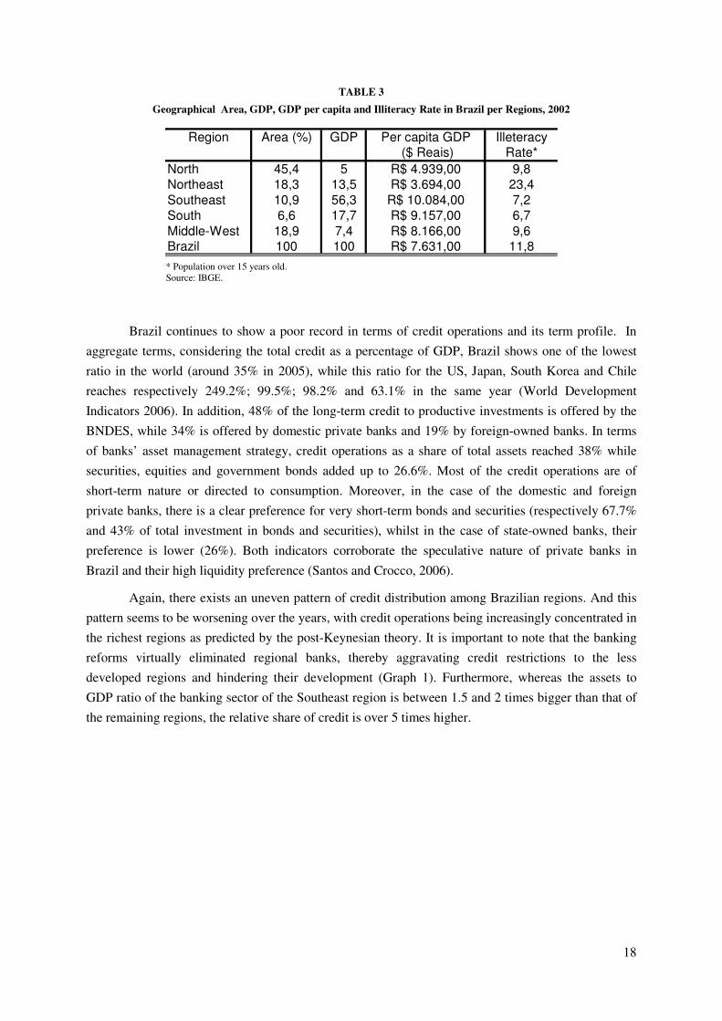
Geographical Area, GDP, GDP per capita and Illiteracy Rate in Brazil per Regions, 2002

Region Area (%) GDP Per capita GDP Illeteracy ($ Reais) Rate*

North 45,4 5 R$ 4.939,00 9,8Northeast 18,3 13,5 R$ 3.694,00 23,4Southeast 10,9 56,3 R$ 10.084,00 7,2South 6,6 17,7 R$ 9.157,00 6,7Middle-West 18,9 7,4 R$ 8.166,00 9,6Brazil 100 100 R$ 7.631,00 11,8

* Population over 15 years old.

Source: IBGE.

Brazil continues to show a poor record in terms of credit operations and its term profile. In

aggregate terms, considering the total credit as a percentage of GDP, Brazil shows one of the lowest

ratio in the world (around 35% in 2005), while this ratio for the US, Japan, South Korea and Chile

reaches respectively 249.2%; 99.5%; 98.2% and 63.1% in the same year (World Development

Indicators 2006). In addition, 48% of the long-term credit to productive investments is offered by the

BNDES, while 34% is offered by domestic private banks and 19% by foreign-owned banks. In terms

of banks’ asset management strategy, credit operations as a share of total assets reached 38% while

securities, equities and government bonds added up to 26.6%. Most of the credit operations are of

short-term nature or directed to consumption. Moreover, in the case of the domestic and foreign

private banks, there is a clear preference for very short-term bonds and securities (respectively 67.7%

and 43% of total investment in bonds and securities), whilst in the case of state-owned banks, their

preference is lower (26%). Both indicators corroborate the speculative nature of private banks in

Brazil and their high liquidity preference (Santos and Crocco, 2006).

Again, there exists an uneven pattern of credit distribution among Brazilian regions. And this

pattern seems to be worsening over the years, with credit operations being increasingly concentrated in

the richest regions as predicted by the post-Keynesian theory. It is important to note that the banking

reforms virtually eliminated regional banks, thereby aggravating credit restrictions to the less

developed regions and hindering their development (Graph 1). Furthermore, whereas the assets to

GDP ratio of the banking sector of the Southeast region is between 1.5 and 2 times bigger than that of

the remaining regions, the relative share of credit is over 5 times higher.

19

GRAPH 1

Spatial Distribution of Credit among Brazilian Regions, 1989-2006

0,00

10,00

20,00

30,00

40,00

50,00

60,00

70,00

80,00

1989 1990 1991 1992 1993 1994 1995 1996 1997 1998 1999 2000 2001 2002 2003 2004 2005 2006

North South Centre-West Northeast Southeast

Source: LEMTe.

We also calculated the Regional Credit Quocient (QCR), which consists of the ratio between

the relative share of a region on the total volume of credit conceded in the country and the relative

share of the same region in the GDP.9 If the index is larger than one, the region’s credit concession is

proportionally larger than what it would be expect given its weight on GDP. Hence, the index allows

us to assess whether the Southeast’s share in total credit is a mere reflection of its economic weight.

The evolution of the QRC is shown in Graph 2 below. It is evident that the North, Northeast and South

regions’ share in credit distribution is lower than their respective contributions to the GDP10

. On the

other hand, the contrary can be observed for the Southeast and Centre-West, the latter being

influenced by the presence of federal banks.

9 The index is a modified version of the location quotient, commonly found in the regional economics literature.

10 The only exception is the North region in 1997, which is explained by isolated facts, most likely the privatization of

Electricity Company of Pará and mining investments in Carajás.

20

GRAPH 2

Regional Quocient of Credit (QRC, %Credit/%GDP)

Source: LEMTe.

TABLE 4

Average Workforce, Bank Branches per capita, Credit Supply per capita, Taxes on Financial Operations (IOF) per capita and Average Wage in Brazil per Regions, 2002

Region Average

workforce

Branches per

capita

Credit

per capita

IOF

per capita Average wage

Northeast 4251 3.70 167.87 32.07 550.09

Southeast 12740 14.49 912.77 133.76 761.01

South 7882 22.43 1693.79 115.20 790.00

Centre-West 5474 11.32 1570.81 107.88 723.52

Note: The Northern region was excluded as explained in section II.

Source: Authors’ elaboration based on data from LEMTe and RAIS/MTE.

In order to further investigate the spatial distribution of the financial system in 2006 we

present in Illustrations 1 to 5 the Local Indicator of Spatial Association i.e. the local Moran’s I at 5%

of significance level (Anselin, 1995).

Illustration 1 shows that there is no clear spatial pattern in the spatial distribution of taxes on

financial operations per capita in 2006. At the Southeastern portion of Brazil there are some small

areas where a positive spatial association with high values can be found. Meanwhile, at the

Northeastern portion, most significant spatial patterns represent a negative spatial association, of the

High-Low type, indicating that municipalities with high values of taxes on financial operations tend to

be surrounded by municipalities with low values, i.e. the financial operations tend to be concentrated

into one locality only in a small region.

21

Illustration 1

Local Moran’s I of the taxes on financial operations per capita, year 2006

N

EW

S

800 0 800 1600 2400 KmLegend:High-HighLow-LowLow-HighHigh-Low

Illustration 2 presents a clearer spatial pattern of positive association of credit supply per

capita at the Brazilian Southeastern region in 2006 while the Northeastern region once again presents a

negative spatial association pattern. This result indicates that the credit supply tends to be less

concentrated in unique localities at the Southeast, spreading with high values over some regions, like

the regions surrounding Rio de Janeiro, the state of São Paulo, among others. However, as it was for

the taxes on financial operations, the credit supply at the Northeast is highly concentrated on single

municipalities in a High-Low pattern.

22

Illustration 2 – Local Moran’s I of the credit supply per capita, year 2006

– N

EW

S

800 0 800 1600 2400 KmLegend:High-HighLow-LowLow-HighHigh-Low

Illustration 3 presents the spatial association of the number of bank branches per capita in

2006. While the spatial association pattern at the Southeastern region is much similar to the credit

supply, there is a positive spatial association of low values at the Northeastern region. Hence,

regarding the number of bank branches per capita we have a spatial concentration of high values at the

Southeastern region and a spatial concentration of low values at the Northeastern region, with some

High-Low outliers which concentrate the bank agencies. As presented in Table 3, the South and

Southeast regions concentrate almost 74% of all bank branches in Brazil.

23

ILLUSTRATION 3

– Local Moran’s I of the number of bank agencies per capita, year 2006

–

Legend:High-HighLow-LowLow-HighHigh-LowKm240016008000800

N

EW

S

Illustration 4 and 5 show the spatial association of the number of employees in the formal

sector and the average wage. Illustration 4 shows a clear imbalance in the spatial distribution of the

average wage in Brazil. While the Southeastern region presents a spatial pattern of high wages, the

Northeastern municipalities represent a cluster of low wages.

Regarding the spatial association of the number of employees in the formal sector, Illustration

5 presents a fuzzy spatial pattern. Some small areas present clusters of high values while others

present cluster of low values surrounded by a large number of outliers presenting a negative spatial

association.

24

ILLUSTRATION 4

Local Moran’s I of the average wage, year 2006

N

EW

S

800 0 800 1600 2400 KmLegend:High-HighLow-LowLow-HighHigh-Low

ILLUSTRATION 5

Local Moran’s I of the general workforce, year 2006

N

EW

S

800 0 800 1600 2400 KmLegend:High-HighLow-LowLow-HighHigh-Low

25

From these statistical analyses made above a first conclusion emerges. The financial variables

related to the management of the bank system (taxes on financial operations and the supply of credit)

have a clear regional pattern which is different from the spatial pattern verified for the variables that

captures the economy as a whole (average wage and number of employees). The high-low pattern in

the northeast (both for financial operations and for credit) is an evidence that bank system in that

region has a higher degree of centrality than that observed in the other regions, specially the southeast.

This degree of centrality is manifested in the high level of spatial concentration of the financial

variables.

IV. ESTIMATIVE AND INFERENCE

The first estimated model is related to the tax on financial operations (IOF). The model

captures the relationship between the per capita amount of tax paid at the bank branches in a

municipality and the amount paid at branches in the neighborhood. The controlling variables are the

number of employees in the municipality, the number of bank branches for each 100,000 citizens, the

average wage and average schooling.

For reference only, Estimation 1 presents the results of a simple IV estimation. This estimation

does not consider the spatial dependence in the error process nor the time-invariant effects.

Meanwhile, Estimation 2 presents the results of the spatial panel model. The results suggest a

negative relationship between the amount of taxes paid in a municipality and the amount paid in the 8

nearest neighbors. This suggests a negative spatial association of the amount of financial operations. If

one municipality has a high level of financial operations, its neighborhood tends to have a lower level,

indicating a spatial concentration of the financial activities. More specifically, an increase of 1% in the

amount of taxes on financial operations paid in the neighborhood is related to a decrease of 0,29% of

the amount paid in one municipality. All the controlling variables presented the expected signs and are

very statistically significant as well. The number of employees and number of bank branches are

positively related to the amount of financial operations, as is the average wage level.

26

TABLE 5

Results of the estimations over the dependent variables IOF and Credit

Estimation 1 Ln_IOF

Estimation 2 Ln_IOF

Estimation 3 Ln_Credit

Estimation 4 Ln_Credit

Intercept -6.4537 -6.3542 -7.6624 -7.7603

(0.1507) (0.3429) (0.1675) (0.4251)

W_Ln_IOF -0.3863 -0.2955 - -

(0.0113) (0.0330)

W_Ln_credit - - -0.1506 -0.1452

(0.0079) (0.0274)

Ln_agencies 0.8138 0.7385 1.2731 1.1945

(0.0082) (0.0202) (0.0092) (0.0251)

Ln_workforce 0.7221 0.7852 0.8847 0.9605

(0.0063) (0.0169) (0.0070) (0.0209)

Ln_wage 0.5198 0.4244 0.5391 0.4931

(0.0272) (0.0577) (0.0301) (0.0715)

Lambda - -0.8517 - -0.6314

Σv - 0.8997 - 0.5316

σ1 - 24.1286 - 37.3908

R² 0.4899 0.5010 0.6102 0.6108

Instruments: Ln_agencies, Ln_workforce, Ln_wage, W_Ln_agencies, W_Ln_workforce,

W_Ln_wage.

Considering the amount of credit supplied by the banks, the negative spatial association

pattern remains, although with a lesser intensity (Estimation 3 and 4). Estimation 3 is for reference

only and presents the results of an IV estimation disregarding the timely and spatial dependence in the

error. Estimation 4 presents the results of the spatial panel estimation. The results suggest a negative

relationship between the amount of credit per capita in a municipality and the amount of credit in the 8

nearest neighbors. As with the financial operations, if one municipality has a high level of credit

release, its neighborhood tends to have a lower level, indicating a spatial concentration of the financial

activities. More specifically, an increase of 1% of the credit in the neighborhood is related to a

decrease of 0,14% of the amount lent in one municipality. Once again, the number of employees and

number of bank branches for each 100,000 citizens are positively related to the amount of credit, as is

the average wage. All variables are statistically significant at a 5% level.

Comparing both results we conclude that the taxes on financial operations (IOF) and the credit

supply present a negative spatial association pattern, in the way that both are spatially concentrated as

would be expected by the propositions of the Central Place Theory. However, it is worthy of mention

that the parameter which measures this spatial association is lower for the IOF. This suggests that the

spatial concentration of financial operations is even higher than the spatial concentration of credit

supply. Hence, under the light of the Central Place Theory, the financial operations have a higher

centrality than the credit supply.

27

FINAL REMARKS

Our theoretical and empirical analyses do not intend to be comprehensive or definitive, but rather

to stimulate further research in this somewhat neglected area. However, they point to important

conclusions and new themes for future research.

1. The spatial structure of financial system was shown to be capable of being understood by

combining the contributions of the New-Keynesian and Post-Keynesian theories with Central-

Place theory;

2. The existence of a negative spatial association between the Brazilian municipalities’ financial

system (in the way that a municipality with more developed financial system tends to be

surrounded by municipalities with less developed financial systems) shows the validity of the

Central Place theory to explain the spatial configuration of the Brazilian financial system;

3. Taking both methods of analyses into consideration (Moran’s-I and the spatial econometrics) it is

possible to state that the Brazilian bank system has a regional pattern of balance sheet

management. The Moran’s I shows a similar spatial pattern for the taxes on financial operations

(IOF) and the supply of credit, with a clear distinctive pattern between the Northeast and the

Southeast regions. This statement is more evident when the econometric results are taken into

consideration. The fact that both the IOF and the supply of credit show negative spatial

correlation reinforces the understanding of these variables as having a strong centrality feature,

which, in turn, is essentially a regional phenomenon.

4. Even recognising that new electronic and information and communication technologies have

dramatically reduced the costs of the exchange of information and thus the friction of distance,

uneven patterns of spatial distribution of credit and financial services (approximated by IOF)

within a country are still observed. In this case as the New-Keynesian and Post-Keynesian

theories have shown, the scale-sensitiveness of the transaction and information costs in the

financial system and the importance of liquidity preference and fundamental uncertainty has

discouraged the proliferation of central-points and led the concentration of financial system

activities, institutions and functions in a few centres at the expense of its periphery;

5. The configuration of the Brazilian financial system may compromise the flow of information

between the firms and the public of the periphery and the financial system in the centre. This may

adversely affect the periphery’s awareness of financing options in the centre and the collection of

information by the centre about the periphery;

6. The results of the model may be interpreted as indicating that the costs of financial activities vary

substantially across municipalities, most notably among different hierarchical levels. Further

research is necessary to explore this aspect.

7. The fact that our results indicate that the Central Place Theory may fit well to explain the spatial

configuration of the Brazilian financial system opens a line of enquiry regarding the development

of a method to create a hierarchy of central places based upon the spatial structure and

development of financial institutions.

28

REFERENCES

Acharya, V., Hasan, I. & Saunders, A. (2002) The Effects of Focus and Diversification on Bank Risk

and Return: evidence from individual bank loan portfolios, CEPR Discussion Papers, CEPR

Discussion Papers, 3252.

Alessandrini, P. & Zazzaro, A. (1999) A ‘Possibilist’ Approach to Local Financial Systems and

Regional Development: the Italian experience. In: Martin, R. (ed.) Money and the Space Economy,

New York, John Wiley and Sons.

Alessandrini, P., Presbitero, A. & Zazzaro, A. (2007) Bank Size or Distance: what hampers innovation

adoption by SMEs?, Working Papers, 304, Universitá Politecnica delle Marche, Dipartimento di

Economia.

Alessandrini, P., Presbitero, A. & Zazzaro, A. (2009) Banks, Distances and Firms’ Financing

Constraints, Review of Finance, 13(2), 261-307.

Anselin, L. (1995) Local Indicators of Spatial Association – LISA, Geographical Analysis, 27(2), 93-

115.

Berger & DeYoung (2001) The Effects of Geographic Expansion on Bank Efficiency, Finance and

Economics Discussion Series, 2001-03, Board of Governors of the Federal Reserve System (U.S.).

Bias P. (1992) Regional financial segmentation in the United States, Journal of Regional Science,

32(3), 321-34.

Bowden, R. & Turkington, D. (1990) Instrumental Variables, Cambridge, Cambridge University

Press.

Brevoot & Hannan (2006) Commercial Lending and Distance: evidence from community

reinvestment act data, Journal of Money, Credit and Banking, 38(8), 1991-2012.

Carling & Lundenberg (2005) Asymmetric information and distance: an empirical assessment of

geographical credit rationing, Journal of Economics and Business, 57(1), 39-59.

Chick, V. & Dow, S. (1988) A Post-Keynesian Perspective on the Relation Between Banking and

Regional Development. In: Arestis, P. (ed) Post Keynesian Monetary Economics, Elegar,

Aldershot.

Christäller, W. (1966) Central places in southern Germany, Englewood Cliffs, Prentice-Hall.

Crocco, M. & Figueiredo, A. (2008) Regional Banking Strategy: an introductory note for the Brazilian

case, 10th International Post Keynesian Conference, Kansas.

Crocco, M. (1999) Uncertainty, Technical Change and Effective Demand, Ph.D. Thesis, London,

University of London.

Crocco, M. (2003) The Concept of Degrees of Unceratinty in Keynes, Shackle and Davidson, Nova

Economia, 12(2), 11-27.

29

Daly, M., Krainer, J. & Lopez, J. (2008) Regional Economic Conditions and Aggregate Bank

Performance. In: Chen, A. (ed) Research in Finance 24, Bingley, Emerald Group Publishing, 103-

27.

Davidson, P. (1982/1983), Rational Expectations: a fallacious foundation for studying crucial

decision-making processes, Journal of Post Keynesian Economics, 5(2), 182-196.

Davidson, P. (1995) Uncertainty in Economics. In Dow S. & Hillard J. (eds.), Keynes, Knowledge and

Uncertainty. Aldershot, Edward Elgar.

Demsetz, R. & Strahan, P. (1997) Diversification, Size, and Risk at U.S. Bank Holding Companies,

Journal of Money, Credit, and Banking, 29(3), 300-313.

Dow, S. (1982) The Regional Composition of the Bank Multiplier Process. In Dow, S. (ed.), Money

and the Economic Process, Aldershot, Elgar.

Dow, S. (1993) Money and the Economic Process, Aldershot, Elgar.

Dow, S. (1996) European Monetary Integration, Endogenous Credit Creation and Regional Economic

Development. In Vence-Deza, X. & Metcalfe, J. (eds) Wealth from Diversity: innovation and

structural change and finance for regional development in Europe, Kluwer, 293-306.

Dow, S. (1999) The Stages of Banking Development and the Spatial Evolution of Financial Systems.

In: Martin, R. (ed.) Money and the Space Economy, New York, John Wiley and Sons, 31-48.

Emmons, W., Gilbert, A. & Yeager, T., (2004) Reducing the Risk at Small Community Banks: is it

size or geographic diversification that matters? Journal of Financial Services Research, 25(2), 259-

281.

Fingleton, B. (2006) Competing models of global dynamics: evidence from panel models with spatially

correlated error components, Regional Science Association International (RSAI) Annual

Conference, Jersey, Channel Islands.

Fingleton, B. (2008) A Generalized Method of Moments Estimator for a Spatial Panel Model with an

Endogenous Spatial Lag and Spatial Moving Average Errors, Spatial Economic Analysis, 3(1), 27-

44.

Furlong, F. & Kreiner, J. (2007) Regional economic conditions and the variability of rates of return in

commercial banking, Federal Reserve Bank of St. Louis Review, 2007-21.

Guiso, L., Sapienza P. & Zingales L. (2002), Does Local Financial Development Matter?, National

Bureau of Economic Research Working Paper, 8922.

Kapoor, M., Kelejian, H. & Prucha, I. (2007) Panel data models with spatially correlated error

components, Journal of Econometrics, 140(1), 97-130.

Kelejian, H. & Prucha, I. (1998) A generalized spatial two-stage least squares procedure for estimating

a spatial autoregressive model with autoregressive disturbances, Journal of Real Estate Finance

and Economics, 17(1), 99-121.

Kelejian, H. & Prucha, I. (1999) A generalized moments estimator for the autoregressive parameter in

a spatial model, International Economic Review, 40(2), 509-533.

30

Klagge, B. & Martin, R. (2005) Decentralized versus centralized financial systems: is there a case for

capital markets, Journal of Economic Geography, 5(4), pages 387-421.

Koo, J. & Moon, H. (2004) Regional Segregation of Financial Markets in Korea, The Bank of Korea

Economic Papers, 46.

Levine, R. (2004) Finance and Growth: theory and evidence, NBER Working Paper Series, 10766.

Martin, R. (1999) Money and the Space Economy, New York, John Wiley and Sons.

Meyer, A. & Yeager, T. (2001) Are Small Rural Banks Vulnerable to Local Economic Downturns?

Federal Reserve Bank of St. Louis Review, 83, 25-38.

Miyakoshi & Tsukuda (2004) Regional Disparities in Japanese Banking Performance, Review of

Urban & Regional Development Studies, 16(1), 74-89.

Morgan & Samolyk (2005) Geographic Diversification in Banking and its Implications for Bank

Portfolio Choice and Performance, mimeo.

Myrdal, G. (1957) Economic Theory and Under-Developed Regions, London, Gerald.

Ozyildirim & Older (2008) Banking Activities and Local Output Growth: does distance from centre

matter? Regional Studies, 42(2), 229-244.

Park, K. & Pennacchi, G. (2009) Harming Depositors and Helping Borrowers: the disparate impact of

bank consolidation, Review of Financial Studies, 22(1), 1-40.

Parr & Budd (2000) Financial Services and the Urban System: an exploration, Urban Studies, 37(3),

593-610.

Samolyk (1994) Bank Performance and Regional Economic Growth: evidence of a regional credit

channel, Federal Reserve Bank of Cleveland Working Paper, 9204.

Santos, F. & Crocco, M. (2006) Financiamento e desenvolvimento sob novas óticas. In: Carvalho, F.

(ed.) A Arquitetura da Exclusão, Observatório da Cidadania nº10, Rio de Janeiro, IBASE.

Usai & Vannini (2005) Banking Structure and Regional Economic Growth: lessons from Italy, The

Annals of Regional Science, 39(4), 691-714.

Valverde & Fernández (2004) The Finance–Growth Nexus: a regional perspective, European Urban

and Regional Studies, 11(4), 339-354.

Yeager, T. (2004) The Demise Of Community Banks? Local Economic Shocks are not to Blame,

Journal of Banking and Finance, 28(9), 2135-2153.