Embed Size (px)
Citation preview
1
Chapter 12: Waiting Lines and Queuing Theory
Models
Textbook: pp. 445-478

2
Learning Objectives (1 of 2)
After completing this chapter, students will be able to:
• Describe the trade-off curves for cost-of-waiting time and
cost of service.
• Describe the basic queuing system configurations and the
three parts of a queuing system: the calling population, the
queue itself, and the service facility.
• Analyse a variety of operating characteristics of waiting lines
for single-channel models with exponential service times
and infinite calling populations.
• Analyse a variety of operating characteristics of waiting lines
for multichannel models with exponential service times and
infinite calling populations.
3
Learning Objectives (2 of 2)
After completing this chapter, students will be able to:
• Analyse a variety of operating characteristics of waiting lines
for single-channel models with deterministic service times
and infinite calling populations.
• Analyse a variety of operating characteristics of waiting lines
for single-channel models with exponential service times and
finite calling populations.
• Understand Little’s Flow Equations.
• Understand the need for simulation for more complex
waiting line models.

4
• Queuing theory is the study of waiting lines
o One of the oldest and most widely used quantitative
analysis techniques
• The three basic components of a queuing process
o Arrivals
o Service facilities
o The actual waiting line
• Analytical models of waiting lines can help managers
evaluate the cost and effectiveness of service systems
Introduction
5
• Most waiting line problems are focused on finding the ideal level of
service a firm should provide
• Generally service level is something management can control
• Often try to find the balance between two extremes
o A large staff and many service facilities
• High levels of service but high costs
o The minimum number of service facilities
• Service cost is lower but may result in dissatisfied
customers
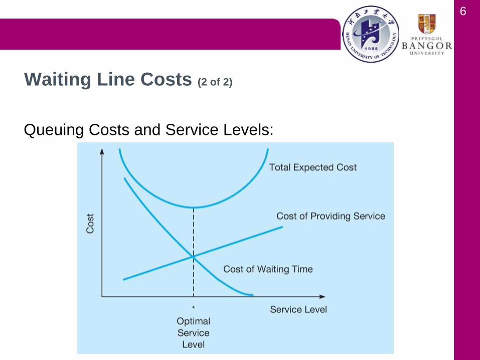
• Service facilities are evaluated on their total expected cost which is
the sum of service costs and waiting costs
o Find the service level that minimises the total expected cost
Waiting Line Costs (1 of 2)
6
Queuing Costs and Service Levels:
Waiting Line Costs (2 of 2)

7
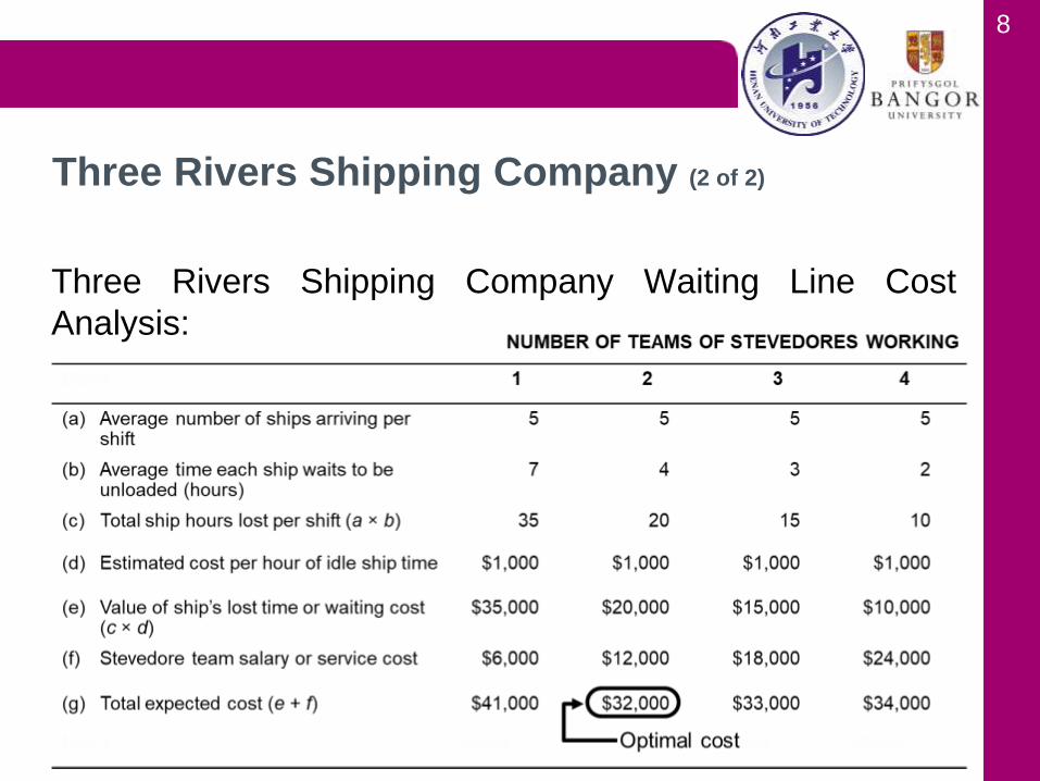
• Three Rivers Shipping operates a docking facility on the
Ohio River
o An average of 5 ships arrive to unload their cargos
each shift
o Idle ships are expensive
o More staff can be hired to unload the ships, but that
is expensive as well
• Three Rivers Shipping Company wants to determine the
optimal number of teams of stevedores to employ each
shift to obtain the minimum total expected cost
Three Rivers Shipping Company (1 of 2)
8
Three Rivers Shipping Company Waiting Line Cost
Analysis:
Three Rivers Shipping Company (2 of 2)

9
• There are three parts to a queuing system
1. Arrivals or inputs to the system (sometimes referred
to as the calling population)
2. The queue or waiting line itself
3. The service facility
• These components have certain characteristics that
must be examined before mathematical queuing models
can be developed
Characteristics of a Queuing System (1 of 10)

10
• Arrival Characteristics have three major characteristics
o Size of the calling population
• Unlimited (essentially infinite) or limited (finite)
• Pattern of arrivals
o Arrive according to a known pattern or can arrive
randomly
o Random arrivals generally follow a Poisson
distribution
Characteristics of a Queuing System (2 of 10)
11
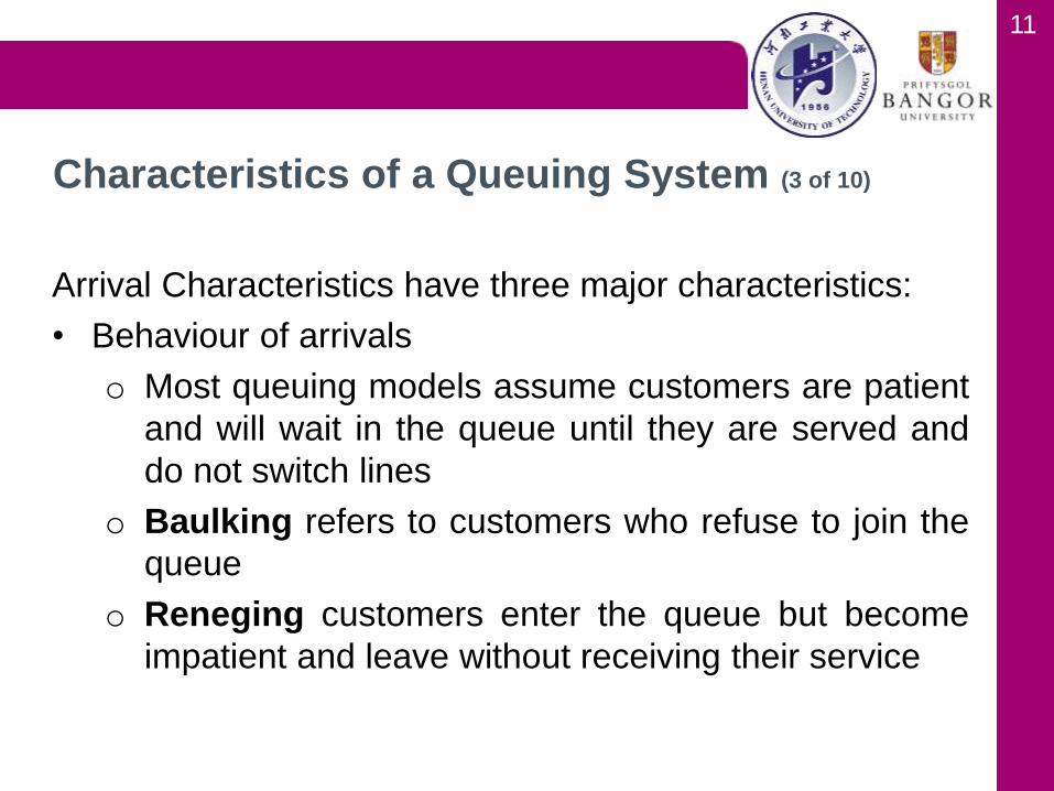
Arrival Characteristics have three major characteristics:
• Behaviour of arrivals
o Most queuing models assume customers are patient
and will wait in the queue until they are served and
do not switch lines
o Baulking refers to customers who refuse to join the
queue
o Reneging customers enter the queue but become
impatient and leave without receiving their service
Characteristics of a Queuing System (3 of 10)

12
Waiting Line Characteristics:
o Can be either limited or unlimited
o Queue discipline refers to the rule by which
customers in the line receive service
o Most common rule is first-in, first-out (FIFO)
o Other rules can be applied to select which customers
enter which queue, but may apply FIFO once they
are in the queue
Characteristics of a Queuing System (4 of 10)

13
Service Facility Characteristics:
1. Configuration of the queuing system
o Single-channel system
• One server
o Multichannel systems
• Multiple servers fed by one common waiting line
Characteristics of a Queuing System (5 of 10)

14
Service Facility Characteristics:
2. Pattern of service times
• Single-phase system
• Customer receives service from just one server
• Multiphase system
• Customer goes through more than one server
Characteristics of a Queuing System (6 of 10)

15
Four Basic Queuing System Configurations:
Characteristics of a Queuing System (7 of 10)
16
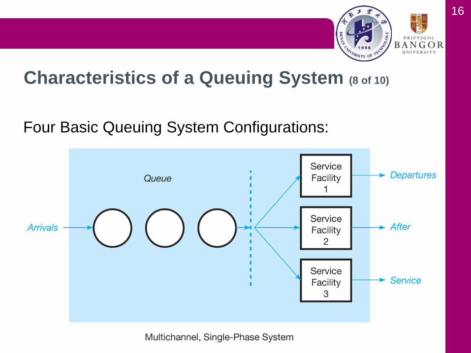
Four Basic Queuing System Configurations:
Characteristics of a Queuing System (8 of 10)

17
Four Basic Queuing System Configurations:
Characteristics of a Queuing System (9 of 10)

18
Service Time Distribution:
• Service patterns can be either constant or random
• Constant service times are often machine controlled
• Generally service times are randomly distributed
according to a negative exponential probability
distribution
• Analysts should observe, collect, and plot service time
data to ensure that the observations fit the assumed
distributions when applying these models
Characteristics of a Queuing System (10 of 10)

19
• A notation for queuing models that specifies the pattern
of arrival, the service time distribution, and the number
of channels
• Basic three-symbol Kendall notation has the form
• Specific letters used to represent probability
distributionsM = Poisson distribution for number of occurrences
D = constant (deterministic) rate
G = general distribution with mean and variance known
Identifying Models Using Kendall Notation (1 of 2)

20
• A single-channel model with Poisson arrivals and
exponential service times would be represented by
M/M/1
• When a second channel is added
M/M/2
• A three-channel system with Poisson arrivals and
constant service time would be
M/D/3
• A four-channel system with Poisson arrivals and
normally distributed service times would be
M/G/4
Identifying Models Using Kendall Notation (2 of 2)

21
Assumptions of the model:
1. Arrivals are served on a FIFO basis
2. There is no baulking or reneging
3. Arrivals are independent of each other but the arrival
rate is constant over time
4. Arrivals follow a Poisson distribution
5. Service times are variable and independent but the
average is known
6. Service times follow a negative exponential distribution
7. Average service rate is greater than the average arrival
rate
Single-Channel Model, Poisson Arrivals and
Exponential Service Times (M/M/1) (1 of 6)

22
Single-Channel Model, Poisson Arrivals and
Exponential Service Times (M/M/1) (2 of 6)
When these assumptions are met, we can develop a series of equations that define thequeue’s operating characteristics

23
Queuing Equations:
Let
λ = mean number of arrivals per time period
μ = mean number of customers or units
served per time period
• The same time period must be used for the arrival rate
and service rate
Single-Channel Model, Poisson Arrivals and
Exponential Service Times (M/M/1) (3 of 6)

24
1. The average number of customers or units in the
system, L
2. The average time a customer spends in the system, W
3. The average number of customers in the queue, Lq
Single-Channel Model, Poisson Arrivals and
Exponential Service Times (M/M/1) (4 of 6)
25
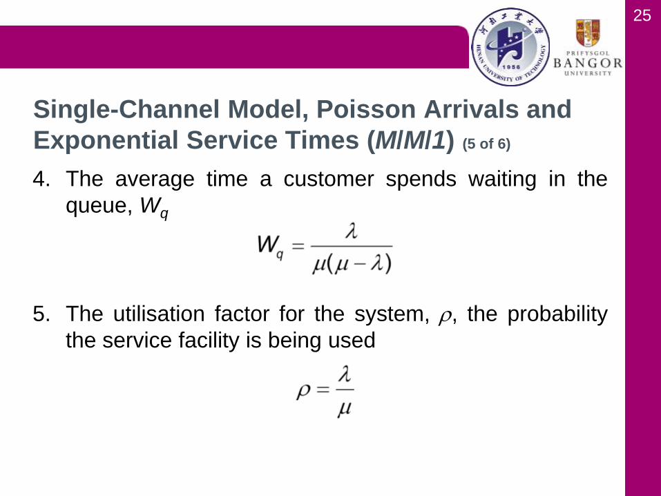
4. The average time a customer spends waiting in the
queue, Wq
5. The utilisation factor for the system, , the probability
the service facility is being used
Single-Channel Model, Poisson Arrivals and
Exponential Service Times (M/M/1) (5 of 6)

26
6. The percent idle time, P0, or the probability no one is in
the system
7. The probability that the number of customers in the
system is greater than k, Pn>k
Single-Channel Model, Poisson Arrivals and
Exponential Service Times (M/M/1) (6 of 6)
27
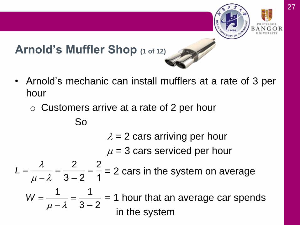
• Arnold’s mechanic can install mufflers at a rate of 3 per
hour
o Customers arrive at a rate of 2 per hour
So
= 2 cars arriving per hour
= 3 cars serviced per hour
= 2 cars in the system on average
= 1 hour that an average car spends
in the system
Arnold’s Muffler Shop (1 of 12)
2 2
3 – 2 1L
1 1
3 – 2W

28
Arnold’s Muffler Shop (2 of 12)
2 22 4
( ) 3(3 – 2) 3(1)qL
1.33 cars waiting in line
on average
2 hour
( ) 3qW
40 minutes average
waiting time per car
20.67
3
percentage of time mechanic
is busy
0
21 1 – 0.33
3P
probability that there are 0
cars in the system

29
• Probability of more than k cars in the system
Arnold’s Muffler Shop (3 of 12)
31
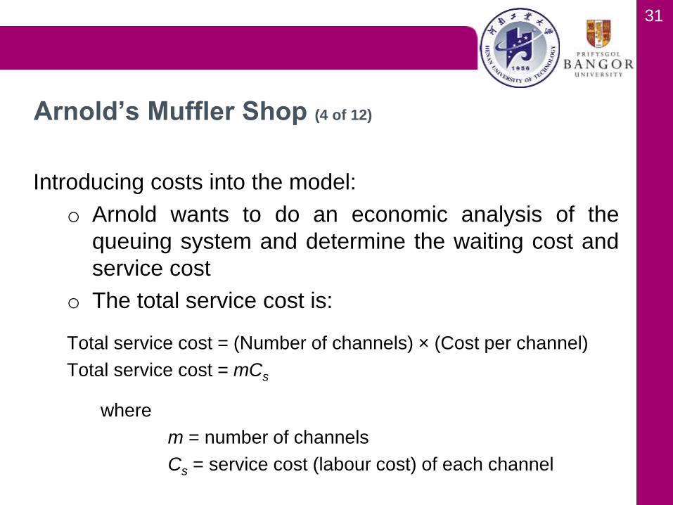
Introducing costs into the model:
o Arnold wants to do an economic analysis of the
queuing system and determine the waiting cost and
service cost
o The total service cost is:
Total service cost = (Number of channels) × (Cost per channel)
Total service cost = mCs
where
m = number of channels
Cs = service cost (labour cost) of each channel
Arnold’s Muffler Shop (4 of 12)

32
• Waiting cost when the cost is based on time in the
system
Total waiting cost = (Total time spent waiting by all arrivals)
× (Cost of waiting)
= (Number of arrivals) × (Average wait per arrival)Cw
Total waiting cost = ( W)Cw
o If waiting time cost is based on time in the queue
Total waiting cost = ( Wq)Cw
Arnold’s Muffler Shop (5 of 12)

33
• So the total cost of the queuing system when based on
time in the system is
Total cost = Total service cost + Total waiting cost
Total cost = mCs + WCw
o And when based on time in the queue
Total cost = mCs + WqCw
Arnold’s Muffler Shop (6 of 12)
34
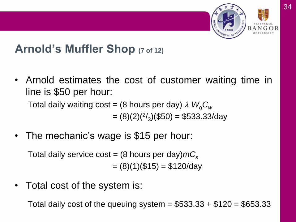
• Arnold estimates the cost of customer waiting time in
line is $50 per hour:
Total daily waiting cost = (8 hours per day) WqCw
= (8)(2)(2/3)($50) = $533.33/day
• The mechanic’s wage is $15 per hour:
Total daily service cost = (8 hours per day)mCs
= (8)(1)($15) = $120/day
• Total cost of the system is:
Total daily cost of the queuing system = $533.33 + $120 = $653.33
Arnold’s Muffler Shop (7 of 12)

35
• Arnold is thinking about hiring a different mechanic who
can install mufflers at a faster rate
o The new operating characteristics would be
= 2 cars arriving per hour
= 4 cars serviced per hour
Arnold’s Muffler Shop (8 of 12)
2 2
4 – 2 2L
1 car in the system on
the average
1 1
4 – 2W
1/2 hour that an average
car spends in the system

36
Arnold’s Muffler Shop (9 of 12)
2 22 4
( ) 4(4 – 2) 8(1)qL
1/2 car waiting in line on
the average
1 hour
( ) 4qW
15 minutes average
waiting time per car
20.5
4
percentage of time mechanic
is busy
0
21 1 – 0.5
4P
probability that there are 0
cars in the system
37
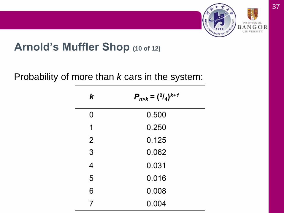
Probability of more than k cars in the system:
Arnold’s Muffler Shop (10 of 12)

38
• The customer waiting cost is the same $50 per hour
Total daily waiting cost = (8 hours per day) WqCw
= (8)(2)(1/4)($50) = $200.00/day
• The new mechanic is more expensive at $20 per hour:
Total daily service cost = (8 hours per day)mCs
= (8)(1)($20) = $160/day
• So the total cost of the system is:
Total daily cost of the queuing system = $200 + $160 = $360
Arnold’s Muffler Shop (11 of 12)

39
• The total time spent waiting for the 16 customers per
day was formerly
(16 cars per day) × (2/3 hour per car) = 10.67 hours
It is now:
(16 cars per day) × (1/4 hour per car) = 4 hours
The total daily system costs are less with the new
mechanic resulting in significant savings:
$653.33 − $360 = $293.33
Arnold’s Muffler Shop (12 of 12)
40
• Reducing waiting time is not the only way to reduce
waiting cost
• Reducing the unit waiting cost (Cw) will also reduce total
waiting cost
• This might be less expensive to achieve than reducing
either W or Wq
Enhancing the Queuing Environment

41
• Equations for the multichannel queuing model
Let
m = number of channels open
= average arrival rate
= average service rate at each channel
Multichannel Model, Poisson Arrivals,
Exponential Service Times (M/M/m) (1 of 4)

42
• Equations for the multichannel queuing model
Let
m = number of channels open
= average arrival rate
= average service rate at each channel
1. The probability that there are zero customers in the
system
Multichannel Model, Poisson Arrivals,
Exponential Service Times (M/M/m) (2 of 4)
0= 1
=0
1 for
1 1
! !
n mn m–
n
P mm
n m m

43
Multichannel Model, Poisson Arrivals,
Exponential Service Times (M/M/m) (3 of 4)
Same basic assumptions as inthe single-channel model!

44
2. The average number of customers or units in the
system
3. The average time a unit spends in the waiting line or
being served, in the system
Multichannel Model, Poisson Arrivals,
Exponential Service Times (M/M/m) (4 of 4)
02
( / )
( – 1)!( )
m
L Pm m
02
( / ) 1
( – 1)!( )
m LW P
m m

45
• The average number of customers or units in line
waiting for service
• The average number of customers or units in line
waiting for service
• The average number of customers or units in line
waiting for service
Single-Channel Model, Poisson Arrivals and
Exponential Service Times (M/M/1)
qL L
1 q
q
LW W
m

46
• Arnold wants to investigate opening a second garage bay
o Hire a second worker who works at the same rate as his
first worker
o Customer arrival rate remains the same
Arnold’s Muffler Shop Revisited (1 of 4)
0 2= 1
=0
1
1 2 1 2 2(3)
! 3 2! 3 2(3) – 2
nn m–
n
P
n
0
1 1 10.5
2 12 1 4 6 21 + + 1 + +
3 33 2 9 6 – 2
P
probability of 0 cars in the system

47
Arnold’s Muffler Shop Revisited (2 of 4)
2
2
82(2)(3)( ) 1 2 1 2 33 3 0.75(1)![2(3) – 2] 2 3 16 2 3 4
Average number of cars in the system
L
3 1 hour 22 minutes28
average time a car spends in the system
LW
3 2 10.083
4 3 12
average number of cars in the queue
qL L
0.0830.0417 hour 2.5 minutes
2
average time a car spends in the queue
q
q
LW
48
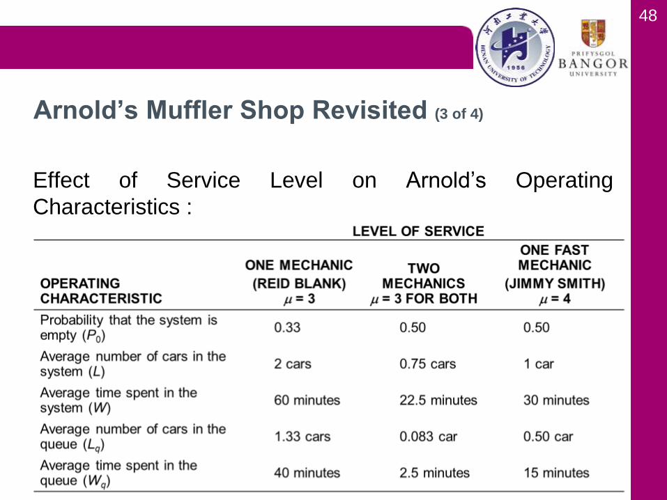
Effect of Service Level on Arnold’s Operating
Characteristics :
Arnold’s Muffler Shop Revisited (3 of 4)

49
• Adding the second service bay reduces the waiting time
in line but will increase the service cost as a second
mechanic needs to be hired
Total daily waiting cost = (8 hours per day) WqCw
= (8)(2)(0.0417)($50) = $33.36
Total daily service cost = (8 hours per day)mCs
= (8)2($15) = $240
Total daily cost of the system = $33.36 + $240 = $273.36
Arnold’s Muffler Shop Revisited (4 of 4)

51
• Constant service times are used when customers or
units are processed according to a fixed cycle
• The values for Lq, Wq, L, and W are always less than
they would be for models with variable service time
o Both average queue length and average waiting time
are halved in constant service rate models
Constant Service Time Model (M/D/1) (1 of 3)

52
• Equations for the Constant Service Time Model
1. Average length of the queue
2. Average waiting time in the queue
Constant Service Time Model (M/D/1) (2 of 3)
2
2 ( )qL
2 ( )qW
53
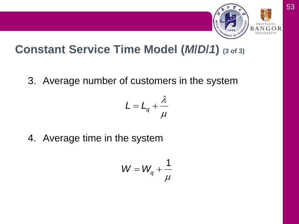
Constant Service Time Model (M/D/1) (3 of 3)
3. Average number of customers in the system
4. Average time in the system
qL L
1qW W

54
• The company collects and compacts aluminum cans
and glass bottles
• Trucks arrive at an average rate of 8 per hour (Poisson
distribution)
• Truck drivers wait about 15 minutes before they empty
their load
• Drivers and trucks cost $60 per hour
• A new automated machine can process truckloads at a
constant rate of 12 per hour
• A new compactor would be amortised at $3 per truck
unloaded
Garcia-Golding Recycling, Inc. (1 of 2)

55
• Analysis of cost versus benefit of the purchase
Current waiting cost/trip = (1/4 hour waiting time)($60/hour cost)
= $15/trip
New system: = 8 trucks/hour arriving
= 12 trucks/hour served
Average waitingtime in queue = Wq = 1/12 hour
Waiting cost/tripwith new compactor = (1/12 hour wait)($60/hour cost) = $5/trip
Savings withnew equipment = $15 (current system) − $5 (new system)
= $10 per tripCost of new equipment
amortised = $3/trip
Net savings = $7/trip
Garcia-Golding Recycling, Inc. (2 of 2)
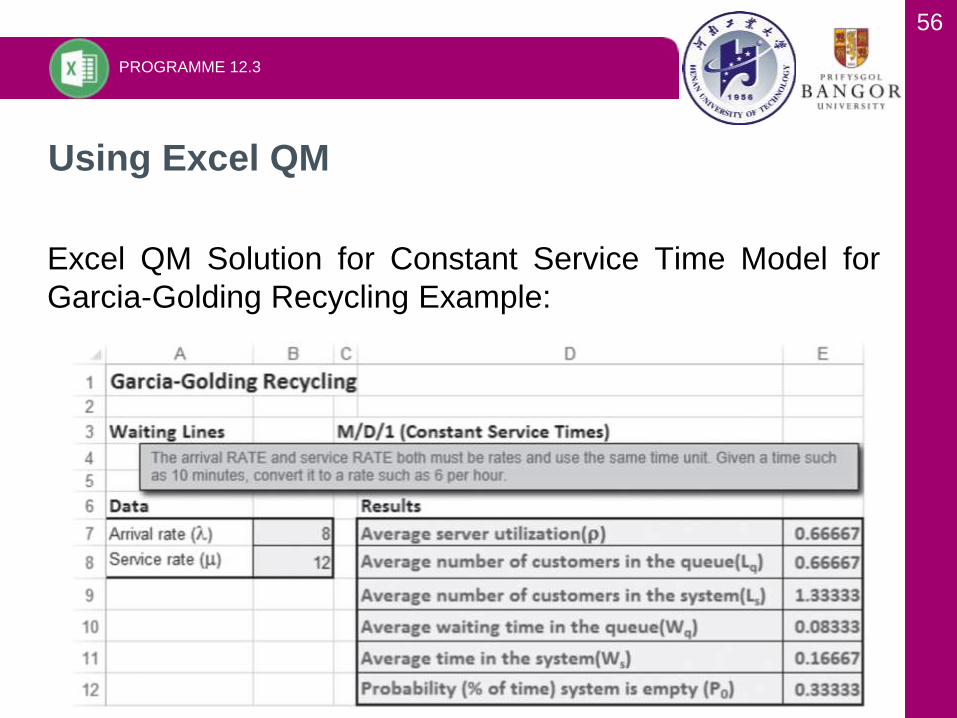
56
Excel QM Solution for Constant Service Time Model for
Garcia-Golding Recycling Example:
Using Excel QM
PROGRAMME 12.3
57
• Models are different when the population of potential
customers is limited
• A dependent relationship between the length of the
queue and the arrival rate
• The model has the following assumptions
1. There is only one server
2. The population of units seeking service is finite
3. Arrivals follow a Poisson distribution and service
times are exponentially distributed
4. Customers are served on a first-come, first-served
basis
Finite Population Model (M/M/1 with Finite
Source) (1 of 4)

58
• Equations for the finite population model
= mean arrival rate
= mean service rate
N = size of the population
1. Probability that the system is empty
Finite Population Model (M/M/1 with Finite
Source) (2 of 4)
0
0
1
!
( )!
nN
n
PN
N – n

59
2. Average length of the queue
3. Average number of customers (units) in the system
4. Average waiting time in the queue
Finite Population Model (M/M/1 with Finite
Source) (3 of 4)
01 – qL N P
01 – qL L P
( )
q
q
LW
N – L

60
5. Average time in the system
6. Probability of n units in the system:
Finite Population Model (M/M/1 with Finite
Source) (4 of 4)
1qW W
0
! for 0,1,...,
!
n
n
NP P n N
N – n
61
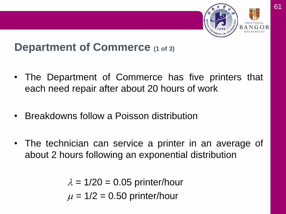
• The Department of Commerce has five printers that
each need repair after about 20 hours of work
• Breakdowns follow a Poisson distribution
• The technician can service a printer in an average of
about 2 hours following an exponential distribution
= 1/20 = 0.05 printer/hour
= 1/2 = 0.50 printer/hour
Department of Commerce (1 of 3)

62
1.
2.
3.
Department of Commerce (2 of 3)
05
=0
10.564
5! 0.05
(5 )! 0.5
n
n
P
n
0
0.05 + 0.55 – 1 0.2 printer
0.05qL P
0.2 + 1 – 0.564 0.64 printerL

63
4.
5.
If printer downtime costs $120 per hour and the technician is paid $25
per hour, the total cost is
Total hourly cost = (Average number of printers down)
(Cost per downtime hour) + Cost per technician
hour
= (0.64)($120) + $25 = $101.80
Department of Commerce (2 of 3)
0.2 0.2
0.91 hour(5 – 0.64) 0.05 0.22
qW
10.91 + 2.91 hours
0.50W
65
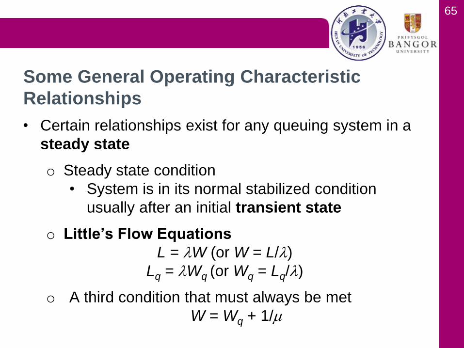
• Certain relationships exist for any queuing system in a
steady state
o Steady state condition
• System is in its normal stabilized condition
usually after an initial transient state
o Little’s Flow Equations
L = W (or W = L/)
Lq = Wq (or Wq = Lq/)
o A third condition that must always be met
W = Wq + 1/
Some General Operating Characteristic
Relationships

66
• Often variations from basic queuing models
• Computer simulation can be used to solve these more
complex problems
o Simulation allows the analysis of controllable factors
o Should be used when standard queuing models
provide only a poor approximation of the actual
service system
More Complex Queuing Models and the Use of
Simulation
67
• End of chapter self-test 1-14
(pp. 469-470)
Compile all answers into one
document and submit at the
beginning of the next lecture!
On the top of the document,
write your Pinyin-Name and
Student ID.
• Please read Chapter 7!
Homework --- Chapter 12


![UTILITIESDIVISION[199] - IowaAnalysis,p.4 Utilities[199] IAC8/26/20 11.11(478) Commonandjointuse 11.12(478) Terminationoffranchisepetitionproceedings 11.13(478) Feesandexpenses](https://img.pdfslide.us/doc/110x75/6024fee3ea0ab15a575dca4a/utilitiesdivision199-iowa-analysisp4-utilities199-iac82620-1111478.jpg)


![[Animebanzai] Bleach 478](https://img.pdfslide.us/doc/110x75/568bd9e31a28ab2034a8b7da/animebanzai-bleach-478.jpg)