Embed Size (px)
Citation preview
CS 478 - Perceptrons 1
CS 478 - Perceptrons 2
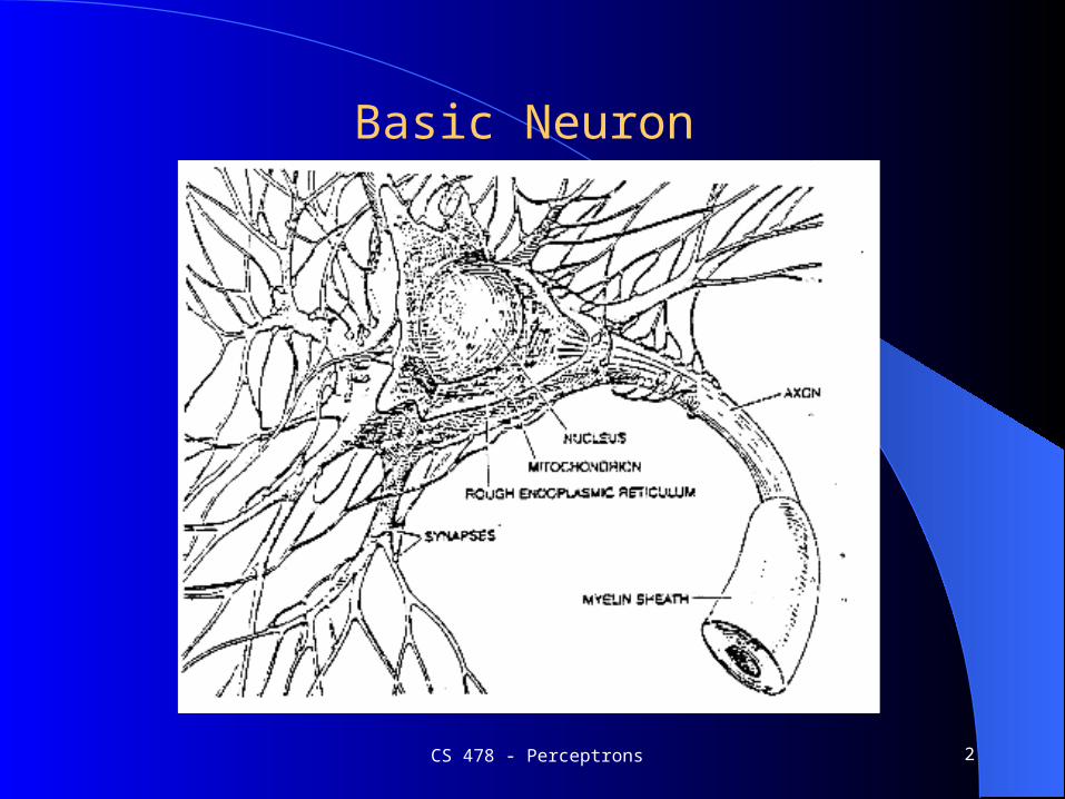
Basic Neuron

CS 478 - Perceptrons 3
Expanded Neuron
CS 478 - Perceptrons 4
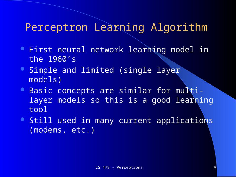
Perceptron Learning Algorithm
First neural network learning model in the 1960’s Simple and limited (single layer models) Basic concepts are similar for multi-layer models so this is
a good learning tool Still used in many current applications (modems, etc.)

CS 478 - Perceptrons 5
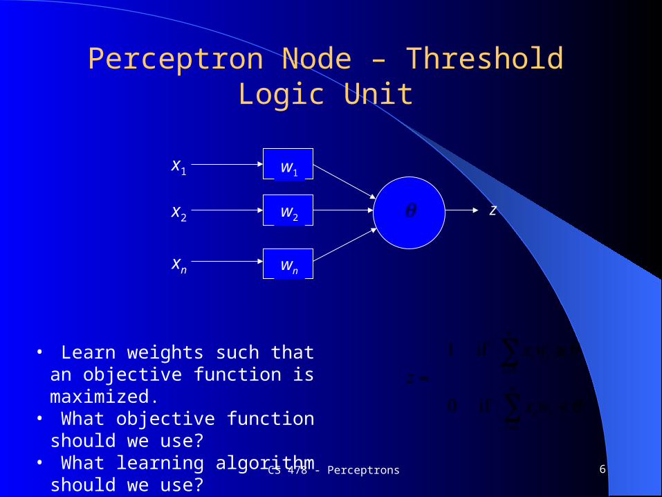
Perceptron Node – Threshold Logic Unit
x1
xn
x2
w1
w2
wn
z
CS 478 - Perceptrons 6
Perceptron Node – Threshold Logic Unit
x1
xn
x2
w1
w2
wn
z
• Learn weights such that an objective function is maximized.
• What objective function should we use?
• What learning algorithm should we use?

CS 478 - Perceptrons 7
Perceptron Learning Algorithm
x1
x2
z
.4
-.2
.1
x1 x2 t
0
1
.1
.3
.4
.8
CS 478 - Perceptrons 8
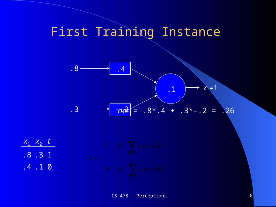
First Training Instance
.8
.3
z
.4
-.2
.1
net = .8*.4 + .3*-.2 = .26
=1
x1 x2 t
0
1
.1
.3
.4
.8
CS 478 - Perceptrons 9
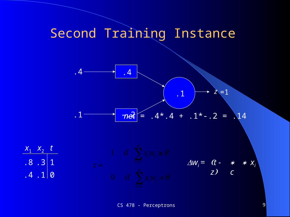
Second Training Instance
.4
.1
z
.4
-.2
.1
x1 x2 t
0
1
.1
.3
.4
.8
net = .4*.4 + .1*-.2 = .14
=1
Dwi = (t - z) * c * xi
CS 478 - Perceptrons 10
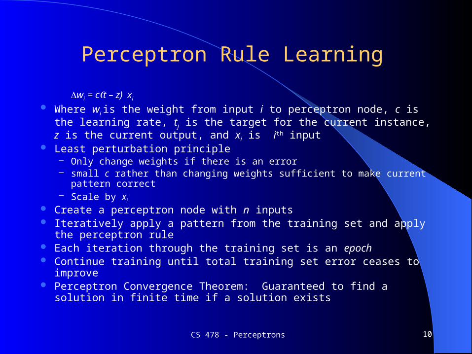
Perceptron Rule Learning
Dwi = c(t – z) xi
Where wi is the weight from input i to perceptron node, c is the learning rate, tj is the target for the current instance, z is the current output, and xi is ith input
Least perturbation principle – Only change weights if there is an error– small c rather than changing weights sufficient to make current pattern correct– Scale by xi
Create a perceptron node with n inputs Iteratively apply a pattern from the training set and apply the perceptron
rule Each iteration through the training set is an epoch Continue training until total training set error ceases to improve Perceptron Convergence Theorem: Guaranteed to find a solution in finite
time if a solution exists
CS 478 - Perceptrons 11
CS 478 - Perceptrons 12
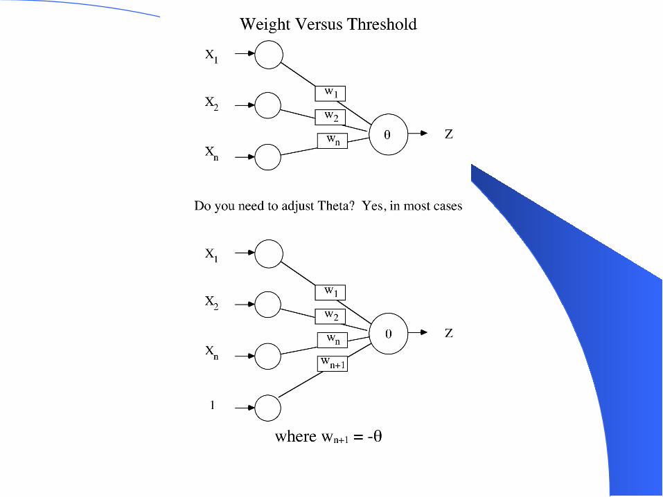
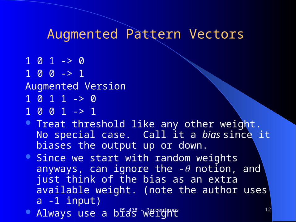
Augmented Pattern Vectors
1 0 1 -> 01 0 0 -> 1Augmented Version1 0 1 1 -> 01 0 0 1 -> 1 Treat threshold like any other weight. No special case.
Call it a bias since it biases the output up or down. Since we start with random weights anyways, can ignore
the - notion, and just think of the bias as an extra available weight. (note the author uses a -1 input)
Always use a bias weight

CS 478 - Perceptrons 13
Perceptron Rule Example
Assume a 3 input perceptron plus bias (it outputs 1 if net > 0, else 0) Assume a learning rate c of 1 and initial weights all 0: Dwi = c(t – z) xi
Training set 0 0 1 -> 01 1 1 -> 11 0 1 -> 10 1 1 -> 0
Pattern Target Weight Vector Net Output DW0 0 1 1 0 0 0 0 0
CS 478 - Perceptrons 14
Example
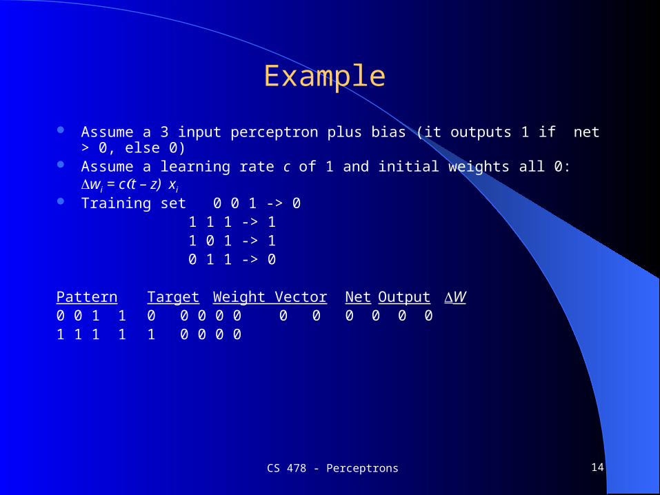
Assume a 3 input perceptron plus bias (it outputs 1 if net > 0, else 0) Assume a learning rate c of 1 and initial weights all 0: Dwi = c(t – z) xi
Training set 0 0 1 -> 01 1 1 -> 11 0 1 -> 10 1 1 -> 0
Pattern Target Weight Vector Net Output DW0 0 1 1 0 0 0 0 0 0 0 0 0 0 01 1 1 1 1 0 0 0 0

CS 478 - Perceptrons 15
Example
Assume a 3 input perceptron plus bias (it outputs 1 if net > 0, else 0) Assume a learning rate c of 1 and initial weights all 0: Dwi = c(t – z) xi
Training set 0 0 1 -> 01 1 1 -> 11 0 1 -> 10 1 1 -> 0
Pattern Target Weight Vector Net Output DW0 0 1 1 0 0 0 0 0 0 0 0 0 0 01 1 1 1 1 0 0 0 0 0 0 1 1 1 11 0 1 1 1 1 1 1 1

CS 478 - Perceptrons 16
Example
Assume a 3 input perceptron plus bias (it outputs 1 if net > 0, else 0) Assume a learning rate c of 1 and initial weights all 0: Dwi = c(t – z) xi
Training set 0 0 1 -> 01 1 1 -> 11 0 1 -> 10 1 1 -> 0
Pattern Target Weight Vector Net Output DW0 0 1 1 0 0 0 0 0 0 0 0 0 0 01 1 1 1 1 0 0 0 0 0 0 1 1 1 11 0 1 1 1 1 1 1 1 3 1 0 0 0 00 1 1 1 0 1 1 1 1
CS 478 - Perceptrons 17
Example
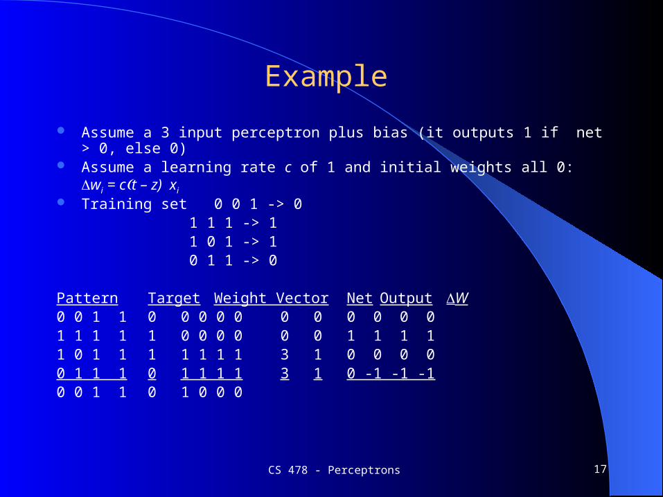
Assume a 3 input perceptron plus bias (it outputs 1 if net > 0, else 0) Assume a learning rate c of 1 and initial weights all 0: Dwi = c(t – z) xi
Training set 0 0 1 -> 01 1 1 -> 11 0 1 -> 10 1 1 -> 0
Pattern Target Weight Vector Net Output DW0 0 1 1 0 0 0 0 0 0 0 0 0 0 01 1 1 1 1 0 0 0 0 0 0 1 1 1 11 0 1 1 1 1 1 1 1 3 1 0 0 0 00 1 1 1 0 1 1 1 1 3 1 0 -1 -1 -10 0 1 1 0 1 0 0 0
CS 478 - Perceptrons 18
Example
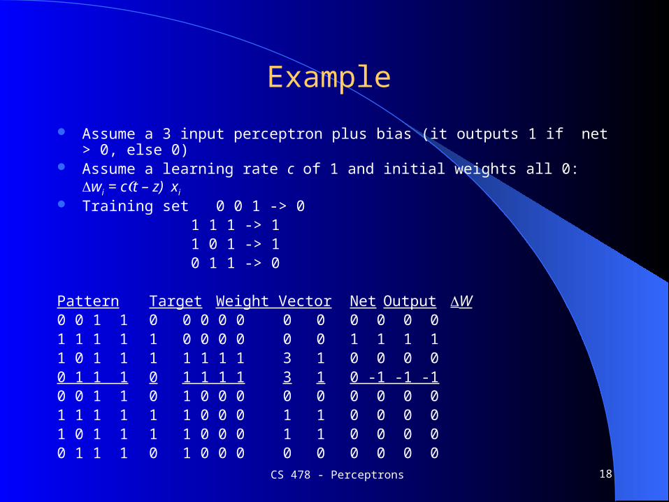
Assume a 3 input perceptron plus bias (it outputs 1 if net > 0, else 0) Assume a learning rate c of 1 and initial weights all 0: Dwi = c(t – z) xi
Training set 0 0 1 -> 01 1 1 -> 11 0 1 -> 10 1 1 -> 0
Pattern Target Weight Vector Net Output DW0 0 1 1 0 0 0 0 0 0 0 0 0 0 01 1 1 1 1 0 0 0 0 0 0 1 1 1 11 0 1 1 1 1 1 1 1 3 1 0 0 0 00 1 1 1 0 1 1 1 1 3 1 0 -1 -1 -10 0 1 1 0 1 0 0 0 0 0 0 0 0 01 1 1 1 1 1 0 0 0 1 1 0 0 0 01 0 1 1 1 1 0 0 0 1 1 0 0 0 00 1 1 1 0 1 0 0 0 0 0 0 0 0 0
CS 478 - Perceptrons 19
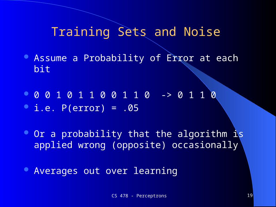
Training Sets and Noise
Assume a Probability of Error at each bit
0 0 1 0 1 1 0 0 1 1 0 -> 0 1 1 0 i.e. P(error) = .05
Or a probability that the algorithm is applied wrong (opposite) occasionally
Averages out over learning
CS 478 - Perceptrons 20
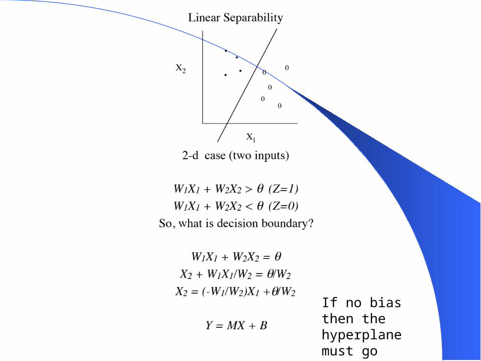
If no bias then the hyperplane must go through the origin
CS 478 - Perceptrons 21
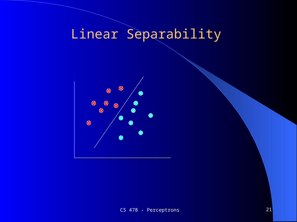
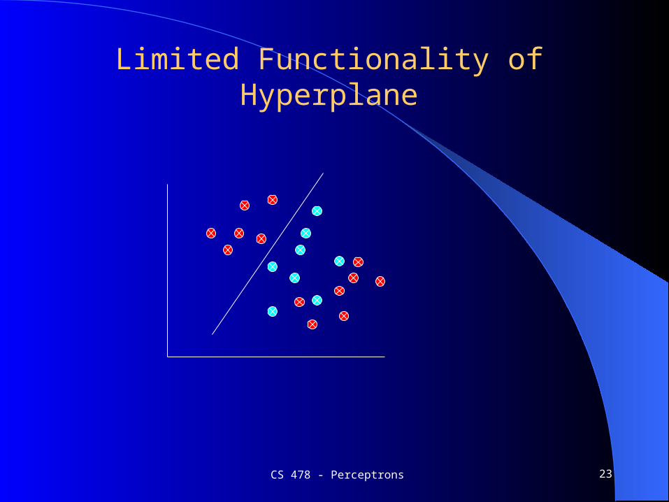
Linear Separability
CS 478 - Perceptrons 22
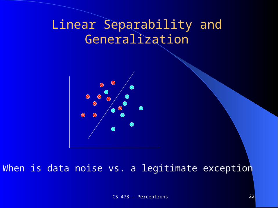
Linear Separability and Generalization
When is data noise vs. a legitimate exception
CS 478 - Perceptrons 23
Limited Functionality of Hyperplane
How to Handle Multi-Class Output This is an issue with any learning model which only
supports binary classification (perceptron, SVM, etc.) Create 1 perceptron for each output class, where the
training set considers all other classes to be negative examples– Run all perceptrons on novel data and set the output to the class of
the perceptron which outputs high– If there is a tie, choose the perceptron with the highest net value
Create 1 perceptron for each pair of output classes, where the training set only contains examples from the 2 classes – Run all perceptrons on novel data and set the output to be the class
with the most wins (votes) from the perceptrons– In case of a tie, use the net values to decide– Number of models grows by the square of the output classes
CS 478 - Perceptrons 24
CS 478 – Perceptrons 25
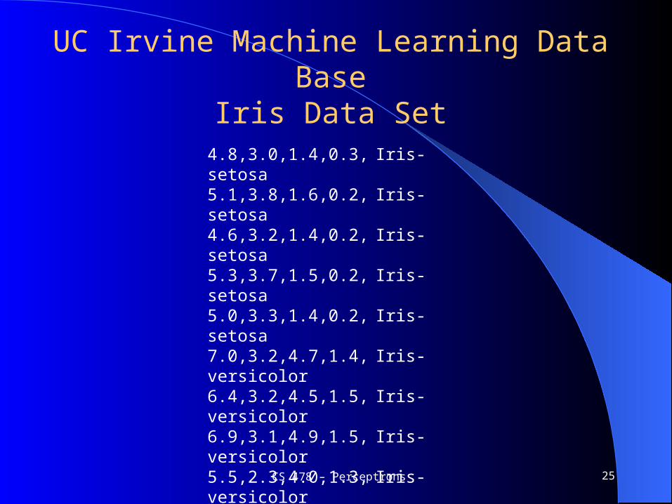
UC Irvine Machine Learning Data BaseIris Data Set
4.8,3.0,1.4,0.3, Iris-setosa5.1,3.8,1.6,0.2, Iris-setosa4.6,3.2,1.4,0.2, Iris-setosa5.3,3.7,1.5,0.2, Iris-setosa5.0,3.3,1.4,0.2, Iris-setosa7.0,3.2,4.7,1.4, Iris-versicolor6.4,3.2,4.5,1.5, Iris-versicolor6.9,3.1,4.9,1.5, Iris-versicolor5.5,2.3,4.0,1.3, Iris-versicolor6.5,2.8,4.6,1.5, Iris-versicolor6.0,2.2,5.0,1.5, Iris-viginica6.9,3.2,5.7,2.3, Iris-viginica5.6,2.8,4.9,2.0, Iris-viginica7.7,2.8,6.7,2.0, Iris-viginica6.3,2.7,4.9,1.8, Iris-viginica
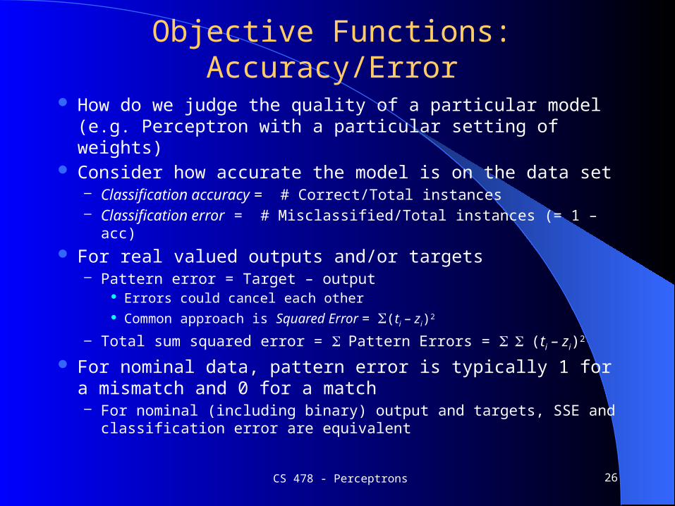
Objective Functions: Accuracy/Error
How do we judge the quality of a particular model (e.g. Perceptron with a particular setting of weights)
Consider how accurate the model is on the data set– Classification accuracy = # Correct/Total instances– Classification error = # Misclassified/Total instances (= 1 – acc)
For real valued outputs and/or targets– Pattern error = Target – output
Errors could cancel each other Common approach is Squared Error = S(ti – zi)2
– Total sum squared error = S Pattern Errors = S S (ti – zi)2
For nominal data, pattern error is typically 1 for a mismatch and 0 for a match– For nominal (including binary) output and targets, SSE and
classification error are equivalent
CS 478 - Perceptrons 26
Mean Squared Error
Mean Squared Error (MSE) – SSE/n where n is the number of instances in the data set– This can be nice because it normalizes the error for data sets of
different sizes– MSE is the average squared error per pattern
Root Mean Squared Error (RMSE) – is the square root of the MSE– This puts the error value back into the same units as the features
and can thus be more intuitive– RMSE is the average distance (error) of targets from the outputs in
the same scale as the features
CS 478 - Perceptrons 27
CS 478 - Perceptrons 28
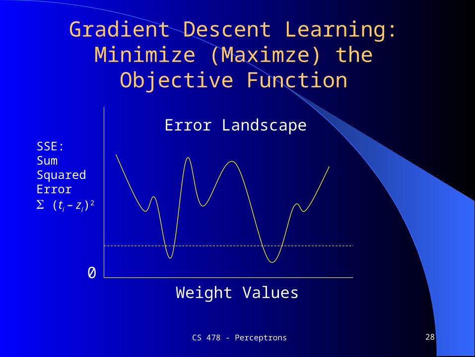
Gradient Descent Learning: Minimize (Maximze) the Objective Function
SSE:Sum SquaredErrorS (ti – zi)2
0
Error Landscape
Weight Values
CS 478 - Perceptrons 29
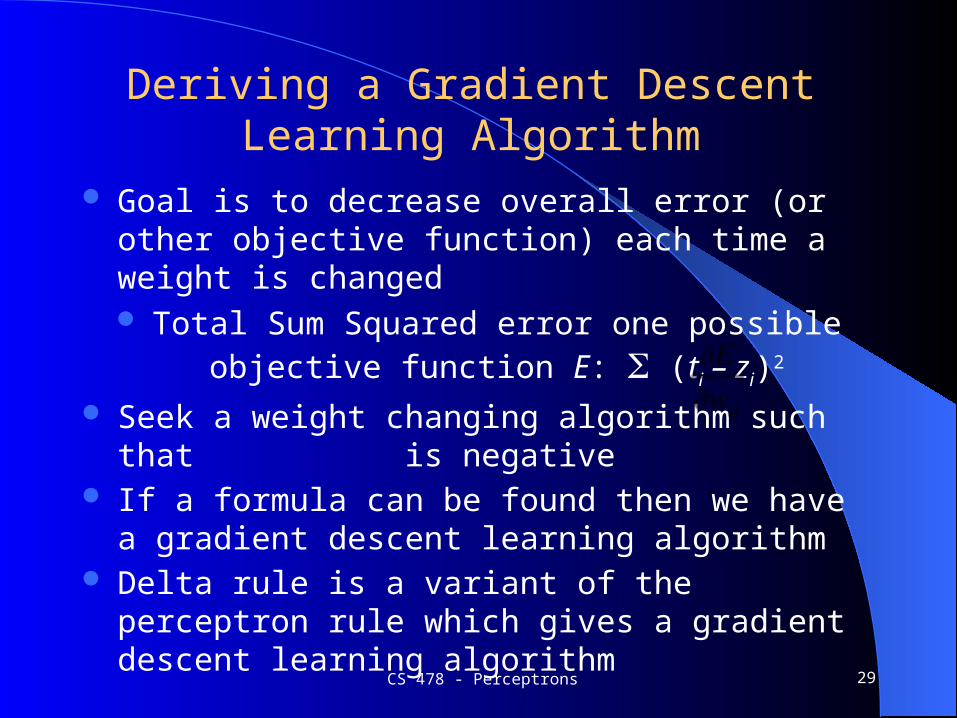
Goal is to decrease overall error (or other objective function) each time a weight is changed
Total Sum Squared error one possible objective function E: S (ti – zi)2
Seek a weight changing algorithm such that is negative
If a formula can be found then we have a gradient descent learning algorithm
Delta rule is a variant of the perceptron rule which gives a gradient descent learning algorithm
Deriving a Gradient Descent Learning Algorithm
CS 478 - Perceptrons 30
Delta rule algorithm
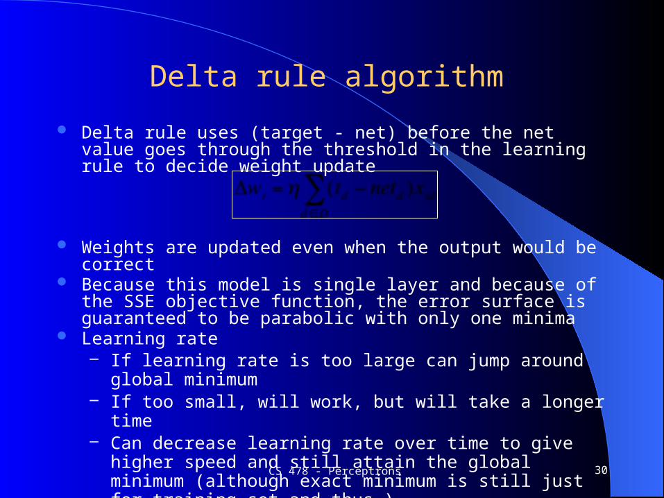
Delta rule uses (target - net) before the net value goes through the threshold in the learning rule to decide weight update
Weights are updated even when the output would be correct Because this model is single layer and because of the SSE objective
function, the error surface is guaranteed to be parabolic with only one minima
Learning rate– If learning rate is too large can jump around global minimum– If too small, will work, but will take a longer time– Can decrease learning rate over time to give higher speed and still
attain the global minimum (although exact minimum is still just for training set and thus…)

Batch vs Stochastic Update
To get the true gradient with the delta rule, we need to sum errors over the entire training set and only update weights at the end of each epoch
Batch (gradient) vs stochastic (on-line, incremental)– With the stochastic delta rule algorithm, you update after every pattern, just like
with the perceptron algorithm (even though that means each change may not be exactly along the true gradient)
– Stochastic is more efficient and best to use in almost all cases, though not all have figured it out yet
Why is Stochastic better? (Save for later)– Top of the hill syndrome– Speed - still not understood by many - talk about later– Other parameters usually make it not true gradient anyways– True gradient descent only in limit of 0 learning rate– Only minima for the training set, exact minima for real task?
CS 478 - Perceptrons 31

CS 478 - Perceptrons 32
Perceptron rule vs Delta rule
Perceptron rule (target - thresholded output) guaranteed to converge to a separating hyperplane if the problem is linearly separable. Otherwise may not converge – could get in cycle
Singe layer Delta rule guaranteed to have only one global minimum. Thus it will converge to the best SSE solution whether the problem is linearly separable or not.– Could have a higher misclassification rate than with the perceptron
rule and a less intuitive decision surface – we will discuss with regression
Stopping Criteria – For these models stop when no longer making progress– When you have gone a few epochs with no significant
improvement/change between epochs (including oscillations)
CS 478 - Perceptrons 33

CS 478 - Perceptrons 34
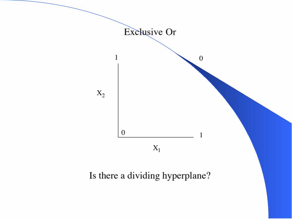
Linearly Separable Boolean Functions
d = # of dimensions
CS 478 - Perceptrons 35
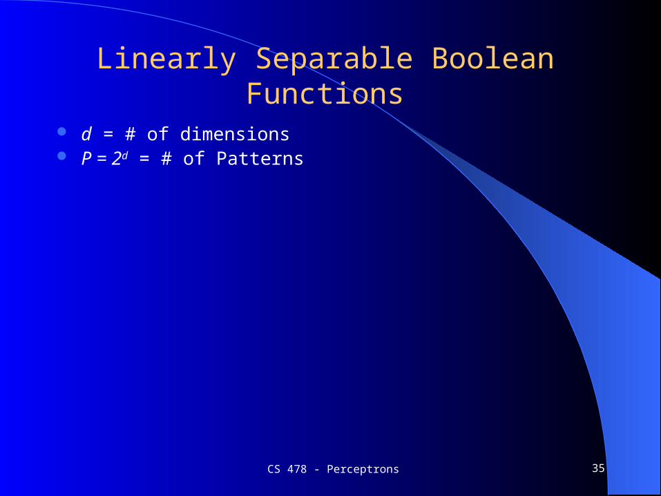
Linearly Separable Boolean Functions
d = # of dimensions P = 2d = # of Patterns
CS 478 - Perceptrons 36
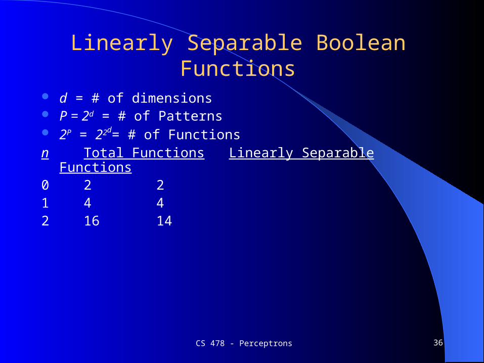
Linearly Separable Boolean Functions
d = # of dimensions P = 2d = # of Patterns 2P = 22d= # of Functionsn Total Functions Linearly Separable
Functions0 2 21 4 42 16 14
CS 478 - Perceptrons 37
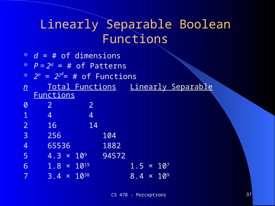
Linearly Separable Boolean Functions
d = # of dimensions P = 2d = # of Patterns 2P = 22d= # of Functionsn Total Functions Linearly Separable
Functions0 2 21 4 42 16 143 256 1044 65536 18825 4.3 × 10⁹ 945726 1.8 × 10¹⁹ 1.5 × 10⁷
7 3.4 × 1038 8.4 × 10⁹

CS 478 - Perceptrons 38
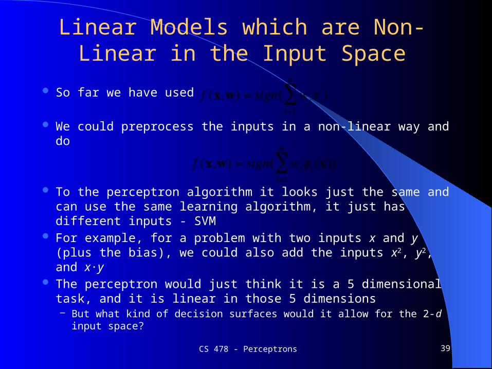
Linear Models which are Non-Linear in the Input Space
So far we have used
We could preprocess the inputs in a non-linear way and do
To the perceptron algorithm it looks just the same and can use the same learning algorithm, it just has different inputs - SVM
For example, for a problem with two inputs x and y (plus the bias), we could also add the inputs x2, y2, and x·y
The perceptron would just think it is a 5 dimensional task, and it is linear in those 5 dimensions– But what kind of decision surfaces would it allow for the 2-d input
space?CS 478 - Perceptrons 39
Quadric Machine
All quadratic surfaces (2nd order)– ellipsoid– parabola– etc.
That significantly increases the number of problems that can be solved, but still many problem which are not quadrically separable
Could go to 3rd and higher order features, but number of possible features grows exponentially
Multi-layer neural networks will allow us to discover high-order features automatically from the input space
CS 478 - Perceptrons 40

Simple Quadric Example
Perceptron with just feature f1 cannot separate the data Could we add a transformed feature to our perceptron?
CS 478 - Perceptrons 41
-3 -2 -1 0 1 2 3 f1

Simple Quadric Example
Perceptron with just feature f1 cannot separate the data Could we add a transformed feature to our perceptron? f2 = f1
2
CS 478 - Perceptrons 42
-3 -2 -1 0 1 2 3 f1
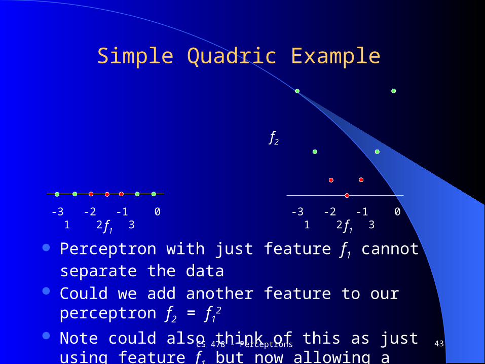
Simple Quadric Example
Perceptron with just feature f1 cannot separate the data
Could we add another feature to our perceptron f2 = f12
Note could also think of this as just using feature f1 but now allowing a quadric surface to separate the data
CS 478 - Perceptrons 43
-3 -2 -1 0 1 2 3 f1
-3 -2 -1 0 1 2 3
f2
f1