Asymptotic Expansions for Large Deviation Probabilities of Noncentral …richter/W-DR2000-1.pdf · 2012-03-27 · Asymptotic Expansions for Large Deviation Probabilities ... generalized

Journal of Multivariate Analysis 75, 184�218 (2000)

Asymptotic Expansions for Large Deviation Probabilitiesof Noncentral Generalized Chi-Square Distributions

W.-D. Richter and J. Schumacher

Universita� t Rostosk, Rostock, Germany

Received June 24, 1997; published online September 22, 2000

Asymptotic expansions for large deviation probabilities are used to approximatethe cumulative distribution functions of noncentral generalized chi-square distribu-tions, preferably in the far tails. The basic idea of how to deal with the tailprobabilities consists in first rewriting these probabilities as large parameter valuesof the Laplace transform of a suitably defined function fk ; second making a seriesexpansion of this function, and third applying a certain modification of Watson'slemma. The function fk is deduced by applying a geometric representation formulafor spherical measures to the multivariate domain of large deviations under con-sideration. At the so-called dominating point, the largest main curvature of theboundary of this domain tends to one as the large deviation parameter approachesinfinity. Therefore, the dominating point degenerates asymptotically. For thisreason the recent multivariate asymptotic expansion for large deviations in Breitungand Richter (1996, J. Multivariate Anal. 58, 1�20) does not apply. Assuming asuitably parametrized expansion for the inverse g~ &1 of the negative logarithm of thedensity-generating function, we derive a series expansion for the function fk . Notethat low-order coefficients from the expansion of g~ &1 influence practically all coef-ficients in the expansion of the tail probabilities. As an application, classificationprobabilities when using the quadratic discriminant function are discussed. � 2000

Academic Press

AMS 1991 subject classifications: 41A60, 41A63, 60F10, 62E17, 62E20, 62H30.Key words and phrases: asymptotic expansion, tail probabilities, noncentral dis-

tribution, spherical distribution, generalized chi-square distribution, geometricrepresentation, large deviations, Watson's lemma, classification probabilities, quadraticdiscriminant function.

1. INTRODUCTION

A commonly made assumption in the theory of statistical models is theuncorrelatedness of the error variables. If the considered population followsa multivariate normal law then the uncorrelatedness of its componentscoincides with their independence. Many statisticians have been trying toallow sampling in cases of dependent but uncorrelated observations, justlike in the class of spherically symmetric distributions. In the present paperwe consider sampling from populations with distributions belonging to this

doi:10.1006�jmva.2000.1899, available online at http:��www.idealibrary.com on

1840047-259X�00 �35.00Copyright � 2000 by Academic PressAll rights of reproduction in any form reserved.

class. Note that it includes both heavy and light tailed sampling distribu-tions such as the Pearson-VII type and Kotz type distributions, respec-tively.

The slightly more general class of elliptically contoured distributions wasinitially studied by Schoenberg (1938) and Kelker (1970). Many authorsafter them contributed to the now quite complex and even matrix variatetheory and gave numerous statistical applications which have beenreviewed recently by Gupta and Varga (1993). Anderson and Fang (1982)considered quadratic forms for elliptically contoured distributions andstudied their central distributions. Cacoullous and Koutras (1984) as wellas Hsu (1990) discussed the corresponding noncentral distributions. In thepresent paper we consider large deviation probabilities for these noncentraldistributions and derive asymptotic representations and expansions forlarge deviation probabilities of noncentral generalized chi-square distribu-tions.

Asymptotic representations as well as saddlepoint approximations forlarge deviation probabilities are shown in several papers, e.g., Daniels(1987), to be good explicit approximations for tail probabilities of statisti-cal distributions. Asymptotic expansions for large deviations in the noncen-tral generalized chi-square distribution are used in Ittrich et al. (2000) formaking statistical inferences concerning the mean in multivariate ellipti-cally contoured distributions. For another application of large deviations inthe noncentral generalized chi-square distribution see the example at theend of this section.

An asymptotic expansion for large deviation of the ordinary central chi-square distribution with k degrees of freedom (d.f.), i.e., for 1&CQ(k)(x)as x � �, can easily be obtained by dealing with the asymptotic behaviorof the one-dimensional Laplace integral

|�

1yk�2&1e&(x�2) y dy

using Laplace's method. General results in this direction can be found inBleistein and Handelsman (1975) as well as Fedorjuk (1977). As anapplication it was shown in Richter and Schumacher (1990) that thecumulative chi-square distribution function satisfies the asymptotic expan-sion formula (in the notation of Bleistein and Handelsman)

1&CQ(k)(c2)tck&2e&c2�2

2k�2&11 \k2+ _1+ :

�

l=1

2l1 \k2+

1 \k2+ c2l& , (1)

185ASYMPTOTIC EXPANSIONS

as c � �, where for k=2m, m # N, we put

1 \k2+

1 \k2

&l+=0 for l>

k2

.

Recognize that if X=(X1 , ..., Xk)T follows the standard Gaussian distribu-tion then

1&CQ(k)(c2)=P(X 21+ } } } +X 2

k>c2),

where X 21 , ..., X 2

k are i.i.d. random variables having a finite moment-generating function. A relation similar to (1) also could therefore be provedusing a suitable saddlepoint technique as in, e.g., Daniels (1987). Thenecessary standard assumptions for applying such techniques, however, arefar from being satisfied if X is distributed according to a non-Gaussianspherically symmetric probability law.

Let CQ(k; g)(x), x # R, denote the cumulative distribution function ofthe g-generalized chi-square distribution, i.e., the distribution of &X&2,where X follows a k-dimensional spherically symmetric distribution withdensity

p(x; g)=C(k, g) g(&x&2), x # Rk,

0<1

C(k, g)=|k |

�

0rk&1g(r2) dr<�,

where |k=2?k�2�1(k�2) denotes the content of the surface area of the unitsphere in Rk.

It is known that the density of &X&2 admits the representation

��r

CQ(k; g)(r)=K(k, g) rk�2&1g(r), r>0,

where K(k, g) is a suitably chosen norming constant.In the same way as was used in Richter and Schumacher (1990), one can

show therefore that if g is of Kotz type, i.e.,

g(r)=rN&1e&;r#, r>0,

186 RICHTER AND SCHUMACHER

for some constants #>0, ;>0, and 2N+k>2, then

1&CQ(k; g)(c2)t;(k+2N&2)�(2#)&1

1 \k+2N&22# +

ck+2N&2&2#e&;c2#

__1+ :�

l=1

dl c&2l#& (2)

as c � �, where

dl=(k+2N&2&2#)(k+2N&2&4#) } } } (k+2N&2&2l#)

(2#;) l .

The noncentral g-generalized chi-square distribution function with k d.f.and noncentrality parameter (n.c.p.) $2>0 can be defined by

CQ(k, $2; g)(x)=P(&X++&2<x), x # R, (3)

for arbitrary + # Rk satisfying &+&2=$2. This distribution was first studiedby Cacoullous and Koutras (1984) and later by Hsu (1990). We start ourconsiderations of large deviations for this distribution from the formula

1&CQ(k, $2; g)(c2)=8(cA$c ; g), c>0, (4)

where 8( } ; g) denotes the probability measure corresponding to the den-sity p( } ; g),

A$c :={x # Rk : "x&\ $�c

ok&1+"�1= , c>0,

and

cA=[(cx1 , ..., cxk)T : (x1 , ..., xk)T # A].

We have thus reformulated the original one-dimensional problem ofevaluating the probabilities 1&CQ(k, $2; g)(c2) as the k-dimensionalproblem to determine the probabilities that a spherically distributed ran-dom vector X falls into the set cA$

c , c>0.Large deviation probabilities for random vectors have been studied by

many authors. Asymptotic expansions for such probabilities can bededuced formally from corresponding expansions for multiple Laplaceintegrals for large parameters. The possibility of expansions of multipleintegrals with boundary maxima is discussed in Bleistein and Handelsman(1975), Fedorjuk (1977), and Wong (1989), but no methods for obtaining


higher-order expansion terms explicitly are outlined there. A geometricapproach to an asymptotic expansion for a certain class of large deviationprobabilities of Gaussian random vectors has been developed recently inBreitung and Richter (1996). This approach is devoted to large deviationdomains with boundaries whose main curvatures near the so-calleddominating points do not change when the large deviation parameterapproaches infinity. The uniquely determined dominating point of the largedeviation domain cA$

c considered above is (c&$, ok&1)T. The largest maincurvature }(c)=1&$�c of the boundary of cA$

c approaches 1 when capproaches infinity. At the same time, the leading term of the expansion inBreitung and Richter (1996) tends to infinity. Hence, this expansion is notapplicable in the present case. We shall develop therefore a new type ofasymptotic expansion for large deviations which will be new even when theunderlying distribution is a Gaussian one.

Example 1 (Classification Probabilities). Let a random vector X followa k-dimensional elliptically contoured distribution such that for some+ # Rk and _>0,

1_

(X&+) td 8( } ; g)

holds. We assume that with +1 {+2 , _21 {_2

2 , the hypotheses

H1 : (+, _2)=(+1 , _21) and H2 : (+, _2)=(+2 , _2

2)

hold true with probabilities p and 1& p, respectively. In accordance withDorflo (1993), let us make the decision that X satisfies H1 if for itsobserved value x, the critical point b=ln(_1(1& p)2�[_2 p2]) and thequadratic discriminant function

Q0(x)=&x&+2&2�_22&&x&+1&2�_2

1

holds

Q0(x)>b.

Recognize that if _21>_2

2 then Q0(x)>b can be rewritten as

&x&�&2>c(b),

where

�=(_21&_2

2)&1 (_21+2&_2

2+1)


and

c(b)=(_21&_2

2)&1 (b_21_2

2+&+1&2 _22&&+2&2 _2

1

+(_21&_2

2)&2 &_21+2&_2

2+1&2).

Let P2(Q0(X)>b) denote the conditional misclassification probability ofdeciding for H1 when H2 is actually true. Then

P2(Q0(X)>b)=P2 \"1_

(X&+)+1_

(+&�)"2

>c(b)_2 +

=8 \{z # Rk : &z+$2&2>c(b)_2

2 =; g+with

$2=1

_2

(+2&�).

It follows that P2(Q0(X)>b) can be written in terms of the noncentralgeneralized chi-square distribution function as

P2(Q0(X)>b)=1&CQ(k, &$2&2; g) \c(b)_2

2 +=1&CQ(k, _2

2 &+1&+2&2�(_21&_2

2)2; g) \c(b)_2

2 + .

Note that if p is ``small' then b and c(b) are ``large.'' For sufficientlylarge c(b), Theorem 3.5 below applies in the sense that the right sideof relation (19) serves as a suitable approximation for P2(Q0(X)>b) ifthe quantities c2 and $2 in (19) are substituted by c(b)�_2

2 and_2

2 &+1&+2&2�(_21&_2

2)2, respectively.

2. ESTIMATES FOR THE LARGE DEVIATION PROBABILITIES

Before deriving the announced asymptotic expansion we will give lowerand upper bounds for the large deviation probabilities

1&CQ(k, $2; g)(c2).


We shall restrict our attention to the case that the density-generating func-tion g admits the representation

g(r)=e&g~ (r), r>0, (D1)

with g~ being first-order continuously differentiable and invertible for larger (r�r2

0). In the main part of what follows we further assume that aparameter *=*(g~ , c) can be chosen in such a way that g~ &1 allows a powerseries expansion in the form

g~ &1(*z+ g~ ((c&$)2))c2 = :

m

j=0

cj z j+O(zm+1), z � 0, (D2, m)

where m is a natural number, the coefficients cj=cj (*, c) approach certainconstants cj* as c tends to infinity,

cj=cj (*, c) � cj , c � �,

and

c1*>0.

From (D2, 0) it follows that

c0=\1&$c+

2

� 1=c0* as c � �.

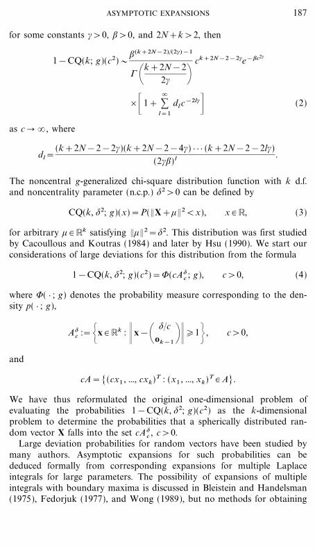
Remark. The coefficients cj depend on the derivatives of g~ at the point(c&$)2. A straightforward proof shows that for m�3,

v c1=*�[c2g~ $((c&$)2)]>0

v c2=&(*�2) c1 g~ "((c&$)2)�[ g~ $((c&$)2)]2

v c3=&(*2�12) c1[ g~ $$$((c&$)2)�[ g~ $((c&$)2)]3&3[ g~ "((c&$)2)]2�[ g~ $((c&$)2)]4].

Example 2 (Kotz Type Density-Generating Function). Since the Kotztype density-generating function has the form

g(r)=rN&1 exp[&;r#], #>0, ;>0, 2N+k>2,

it follows that

g~ (r)=;r#&(N&1) ln r


and we have

c1 =*

c2#

(1&$�c)2

\#; \1&$c+

2#

&N&1

c2# +,

c2=&*2

2c4#

\1&$c+

2

\#(#&1) ; \1&$c+

2#

+N&1

c2# +\#; \1&

$c+

2#

&N&1

c2# +3 ,

and

c3 =&*3

12c6#

\1&$c+

2

\#(#&1)(#&2) ; \1&$c+

2#

&2N&1

c2# +\#; \1&

$c+

2#

&N&1

c2# +4

+*3

4c6#

\1&$c+

2

\#(#&1) ; \1&$c+

2#

+N&1

c2# +2

\#; \1&$c+

2#

&N&1

c2# +5 .

Thus g~ satisfies assumption (D2, m), m=1, 2..., with *=c2#.

Example 3 (Pearson VIII Type Density Generating Function). Sincethe Pearson-VII type density-generating function has the form

g(r)=\1+rm+

&M

, r>0,

for certain constants M>k�2, m>0, it follows that

g~ (r)=M ln \1+rm+

and we have

c1 =*M \m

c2+\1&$c+

2

+ , c2=*2

2M2 \mc2+\1&

$c+

2

+ ,

c3=*3

6M3 \mc2+\1&

$c+

2

+ .


Thus g~ satisfies assumption (D2, m), m=1, 2, ..., with an arbitrary positiveconstant *.

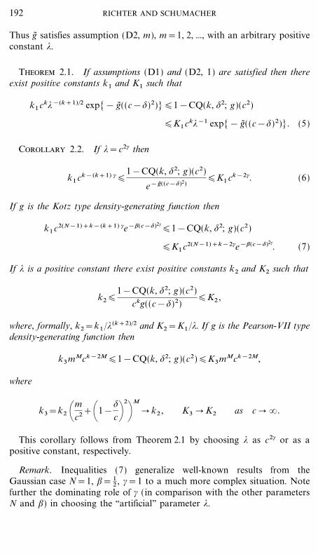
Theorem 2.1. If assumptions (D1) and (D2, 1) are satisfied then thereexist positive constants k1 and K1 such that

k1 ck*&(k+1)�2 exp[& g~ ((c&$)2)]�1&CQ(k, $2; g)(c2)

�K1ck*&1 exp[& g~ ((c&$)2)]. (5)

Corollary 2.2. If *=c2# then

k1 ck&(k+1) #�1&CQ(k, $2; g)(c2)

e&g~ ((c&$)2)�K1 ck&2#. (6)

If g is the Kotz type density-generating function then

k1c2(N&1)+k&(k+1) #e&;(c&$)2#�1&CQ(k, $2; g)(c2)

�K1c2(N&1)+k&2#e&;(c&$)2#. (7)

If * is a positive constant there exist positive constants k2 and K2 such that

k2�1&CQ(k, $2; g)(c2)

ckg((c&$)2)�K2 ,

where, formally, k2=k1�*(k+2)�2 and K2=K1 �*. If g is the Pearson-VII typedensity-generating function then

k3 mMck&2M�1&CQ(k, $2; g)(c2)�K3mMck&2M,

where

k3=k2 \mc2+\1&

$c+

2

+M

� k2 , K3 � K2 as c � �.

This corollary follows from Theorem 2.1 by choosing * as c2# or as apositive constant, respectively.

Remark. Inequalities (7) generalize well-known results from theGaussian case N=1, ;= 1

2 , #=1 to a much more complex situation. Notefurther the dominating role of # (in comparison with the other parametersN and ;) in choosing the `àrtificial'' parameter *.


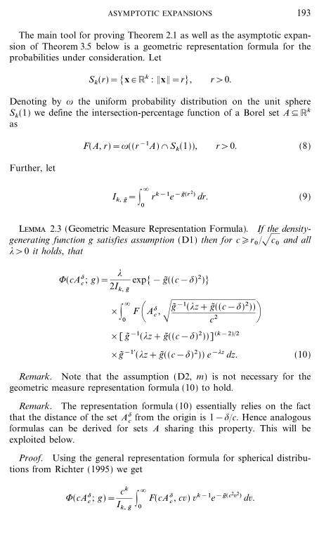
The main tool for proving Theorem 2.1 as well as the asymptotic expan-sion of Theorem 3.5 below is a geometric representation formula for theprobabilities under consideration. Let

Sk(r)=[x # Rk : &x&=r], r>0.

Denoting by | the uniform probability distribution on the unit sphereSk(1) we define the intersection-percentage function of a Borel set A�Rk

as

F(A, r)=|((r&1A) & Sk(1)), r>0. (8)

Further, let

Ik, g~ =|�

0rk&1e&g~ (r 2) dr. (9)

Lemma 2.3 (Geometric Measure Representation Formula). If the density-generating function g satisfies assumption (D1) then for c�r0 �- c0 and all*>0 it holds, that

8(cA$c ; g)=

*2Ik, g~

exp[& g~ ((c&$)2)]

_|�

0F \A$

c , �g~ &1(*z+ g~ ((c&$)2))c2 +

_[ g~ &1(*z+ g~ ((c&$)2))](k&2)�2

_g~ &1$(*z+ g~ ((c&$)2)) e&*z dz. (10)

Remark. Note that the assumption (D2, m) is not necessary for thegeometric measure representation formula (10) to hold.

Remark. The representation formula (10) essentially relies on the factthat the distance of the set A$

c from the origin is 1&$�c. Hence analogousformulas can be derived for sets A sharing this property. This will beexploited below.

Proof. Using the general representation formula for spherical distribu-tions from Richter (1995) we get

8(cA$c ; g)=

ck

Ik, g~|

�

0F(cA$

c , cv) vk&1e&g~ (c2v2) dv.


Since

F(cA$c , cv)#F(A$

c , v), \c>0,

by the definition of the intersection-percentage function F and because

F(A$c , v)#0 for v # _0, 1&

$c+

we have

8(cA$c ; g)=

ck

Ik, g~|

�

1&$�cF(A$

c , v) vk&1e&g~ (c2v2) dv.

For v�1&$�c and c�r0 �- c0 , the relation

g~ (c2v2)=*y

is invertible and the substitution g~ (c2v2)=*y yields

8(cA$c ; g)=

*2Ik, g~

|�

g~ ((c&$)2)�*F \A$

c , �g~ (*y)c2 +

_[ g~ &1(*y)] (k&2)�2 g~ &1$(*y) e&*y dy.

The asserted representation now follows by substituting

z= y& g~ ((c&$)2)�*. K

Proof of Theorem 2.1. Let

AS :=[x # Rk : &x&�1&$�c]

be the complement of a sphere with radius 1&$�c and let

AH :=[x # Rk : x1�1&$�c]

be a halfspace with the same distance from the origin as AS and A $c . Then

AH �A$c �AS

and consequently

8(cAH ; g)�8(cA$c ; g)�8(cAS ; g).


As remarked after Lemma 2.3, geometric measure representation formulae

8(cA; g)=*

2Ik, g~exp[& g~ ((c&$)2)]

_|�

0F \A, �g~ &1(*z+ g~ ((c&$)2))

c2 +_[ g~ &1(*z+ g~ ((c&$)2))](k&2)�2

_g~ &1$(*z+ g~ ((c&$)2)) e&*z dz, (11)

analogous to (10), hold true for the sets A=AH and A=AS as well. Wewill exploit now these formulae to determine the asymptotic behavior ofthe probabilities 8(cAH ; g) and 8(cAS ; g) as c � �.

We start with the derivation of the upper bound. Since

F \AS , �g~ &1(*z+ g~ ((c&$)2))c2 +#1 for z # [0, �],

we have

8(cAS ; g)=ck

2Ik, g~exp[& g~ ((c&$)2)]

_|�

0 _g~ &1(*z+ g~ ((c&$)2))c2 &

(k&2)�2

_��z _

g~ &1(*z+ g~ ((c&$)2))c2 & e&*z dz.

Using assumptions (D1) and (D2, 1), an application of Laplace's methodto the last integral implies

8(cAS ; g)tck

2*Ik, g~exp[& g~ ((c&$)2)] c(k&2)�2

0 c1 , * � �.

Hence

8(cAS ; g) ��ck

*exp[& g~ ((c&$)2)] as * � �. (12)

We now deal with AH . The intersection-percentage function for halfspaceswas determined in Richter (1992) and generalized in Richter (1995). For


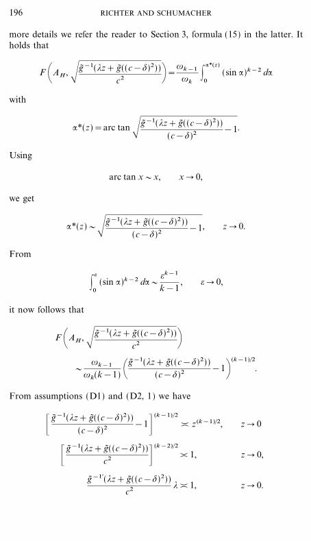
more details we refer the reader to Section 3, formula (15) in the latter. Itholds that

F \AH , �g~ &1(*z+ g~ ((c&$)2))c2 +=

|k&1

|k|

:*(z)

0(sin :)k&2 d:

with

:*(z)=arc tan �g~ &1(*z+ g~ ((c&$)2))(c&$)2 &1.

Using

arc tan xtx, x � 0,

we get

:*(z)t�g~ &1(*z+ g~ ((c&$)2))(c&$)2 &1, z � 0.

From

|=

0(sin :)k&2 d:t

=k&1

k&1, = � 0,

it now follows that

F \AH , �g~ &1(*z+ g~ ((c&$)2))c2 +

t|k&1

|k(k&1) \g~ &1(*z+ g~ ((c&$)2))

(c&$)2 &1+(k&1)�2

.

From assumptions (D1) and (D2, 1) we have

_g~ &1(*z+ g~ ((c&$)2))(c&$)2 &1&

(k&1)�2

�� z(k&1)�2, z � 0

_g~ &1(*z+ g~ ((c&$)2))c2 &

(k&2)�2

�� 1, z � 0,

g~ &1$(*z+ g~ ((c&$)2))c2 * �� 1, z � 0.


These relations, together with an application of Laplace's method, lead tothe asymptotic equivalence

8(cAH ; g) �� ck*&(k+1)�2 exp[& g~ ((c&$)2)], c � �. (13)

This concludes the proof. K

3. MAIN RESULTS

The basic idea of how to deal with the large deviation probabilities of thenoncentral generalized chi-square distributions consists in first rewritingthese large deviation probabilities as large parameter values of the Laplacetransform of a certain parameter-dependent function

y � fk(c, k, y)

defined below, second expanding fk(c, *, y) into a series with respect topowers of y1�2, and third applying a suitable modification of Watson'slemma.

Lemma 3.1 (Laplace Integral Representation). If the density-generatingfunction g satisfies assumption (D1) then for c�r0�- c0 and all *>0 itholds that

1&CQ(k, $2; g)(c2)

=*

2cIk, g~e&g~ ((c&$)2) |

�

0fk(c, *, y) e&(*�c) y dy (14)

with

fk(c, *, y)=F \A$c ,�g~ &1 \*

cy+ g~ ((c&$)2)+

c2 +__g~ &1 \*

cy+ g~ ((c&$)2)+&

(k&2)�2

g~ &1$ \*c

y+ g~ ((c&$)2)+ .

Proof. The assertion of this lemma follows immediately fromLemma 2.3 by substituting z= y�c. K


The essential step in expanding fk is to derive a series representation forthe intersection-percentage function F.

In Ittrich et al. (2000) it is shown that the set A$c belongs to the system

A(dir, dist) of Borel sets defined in Richter (1995) (Fig. 1). In Richter(1995) it is shown that

F(A, r)=|k&1

|k|

:*(r)

0(sin :)k&2 d: (15)

holds for arbitrary A from A(dir, dist), where

:*(r)=arc tan \\ rRA(r)+

2

&1+1�2

and the so-called distance-type function r � RA(r) describes a certaingeometric property of the set A. For the set A=A$

c the function RA hasbeen determined in Ittrich et al. (2000):

RA(r)=c2&$2&c2r2

2$c.

We are now in a position to expand F.

FIG. 1. The sets A$c and A$

c & Sk(r).


Lemma 3.2 (Expansion of the Intersection-Percentage Function). Underthe assumptions (D1) and (D2, m) the intersection-percentage functionadmits the representation

F \A$c , �g~ &1(*y�c+ g~ ((c&$)2))

c2 +=

|k&1

|k:

m&1

j=0

Bj

2 j+k&1y (2 j+k&1)�2+O( y(k&1)�2+m), (16)

as y � 0, for some well-defined constants Bj given explicitly in formula (28)below.

The proof of this lemma is quite technical, and we will therefore leave itto Section 5.

Expansion (16) for the intersection-percentage function combined oncemore with the assumed expansion (D2, m) for g~ &1 leads to an expansionfor the whole function fk .

Lemma 3.3. It holds that

fk(c, *, y)=|k&1

|k

ck

*:

m&1

j=0

bj+1 y(k&1)�2+ j

+O( y(k&1)�2+m), y � 0, (17)

with the first three coefficients bj given explicitly in the proof of (17) inSection 5.

Remarks. Note that low-order coefficients from the expansion of g~ &1

influence all coefficients bj , j= j0 , ..., m, starting from some index j0 .Although the aim of this paper is to derive an expansion in terms of c

we are still dealing here with an expansion in terms of y. Consequently, thecoefficients bj occurring in Lemma 3.3 are not yet ordered with respect tothe powers of c.

Lemma 3.4 (Modified Watson's Lemma). Let f: (0, �)_2 � R satisfythe following assumptions:

(i) f (*, } ) is locally integrable for every *>0 and uniformly (withrespect to *) bounded on finite intervals;

(ii) f (*, y)=O(eay), y � � uniformly in *;


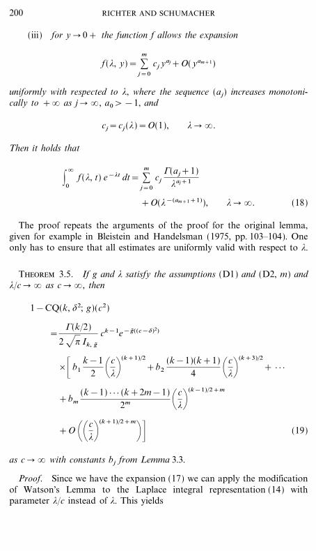
(iii) for y � 0+ the function f allows the expansion

f (*, y)= :m

j=0

cj yaj+O( yam+1)

uniformly with respected to *, where the sequence (aj) increases monotoni-cally to +� as j � �, a0>&1, and

cj=cj (*)=O(1), * � �.

Then it holds that

|�

0f (*, t) e&*t dt= :

m

j=0

cj1(aj+1)

*aj+1

+O(*&(am+1+1)), * � �. (18)

The proof repeats the arguments of the proof for the original lemma,given for example in Bleistein and Handelsman (1975, pp. 103�104). Oneonly has to ensure that all estimates are uniformly valid with respect to *.

Theorem 3.5. If g and * satisfy the assumptions (D1) and (D2, m) and*�c � � as c � �, then

1&CQ(k, $2; g)(c2)

=1(k�2)

2 - ? Ik, g~

ck&1e&g~ ((c&$)2)

__b1

k&12 \c

*+(k+1)�2

+b2

(k&1)(k+1)4 \c

*+(k+3)�2

+ } } }

+bm(k&1) } } } (k+2m&1)

2m \c*+

(k&1)�2+m

+O \\c*+

(k+1)�2+m

+& (19)

as c � � with constants bj from Lemma 3.3.

Proof. Since we have the expansion (17) we can apply the modificationof Watson's Lemma to the Laplace integral representation (14) withparameter *�c instead of *. This yields


1&CQ(k, $2; g)(c2)

=ck&1|k&1

2|k Ik, g~e&g~ ((c&$)2) _ :

m&1

j=0

bj+1

1((k+1)�2+ j)(*�c) (k+1)�2+ j

+O \\c*+

(k+1)�2+m

+&=

ck&1

2 - ? Ik, g~

e&g~ ((c&$)2) 1(k�2)1((k&1)�2)

__b1 1 \k+12 +\c

*+(k+1)�2

+b21 \k+32 +\c

*+(k+3)�2

+b3 1 \k+52 +\c

*+(k+5)�2

+ } } } +bm 1 \k&12

+m+\c*+

(k&1)�2+m

+O \\c*+

(k+1)�2+m

+& .

The assertion follows from using properties of the 1-function. K

Note again that low-order coefficients from the expansion of g~ &1

influence practically all coefficients in the expansion of the tail probabilities1&CQ(k, $2; g)(c2) starting from some index.

Corollary 3.6. If g is the Kotz type density-generating function with#>1�2 then it holds that

1&CQ(k, $2; g)(c2)

=;k�2#+(N&1)�#&(k+1)�21 \k

2+2 - ? #(k&1)�2$(k&1)�21 \ k

2#+

N&1# +

_c(3k&1)�2&#(k+1)+2N&2e&;(c&$)2#

_[1+D1&2#c1&2#+D&2#c&2#+D&1&2#c&1&2#+D2&4#c2&4#

+D1&4#c1&4#+D&4#c&4#+D&1&4#c&1&4#+D&2&4#c&2&4#

+O(c3&6#)], c � �, (20)

with coefficients Dj given explicitly in the proof of (20) in Section 5.

Remarks. In accordance with the remarks after Lemma 3.3 andTheorem 3.5 the coefficients occurring in the expansions of Theorem 3.5


and Corollary 3.6 are not ordered with respect to the powers of c&1.Actually, the value of the parameter # influences the ordering of the expan-sion terms with respect to their rate of convergence to zero as c approachesinfinity. Moreover, the orders of two or more expansion terms can coincidefor special choices of #. Therefore, there is formally no uniqueness in thenotation of the coefficients D� .

If, e.g., #=1 then

1&2#>&2#=2&4#,

max[&1&2#, 1&4#, &4#, &1&4#, &2&4#]=3&6#,

and D&2# and D2&4# are both coefficients of c&2. If in this case we putD*&2=D&2#+D2&4# then the result of Corollary 3.6 can be reformulated as

1&CQ(k, $2; g)(c2)

=;N&3�21 \k

2+2 - ? $(k&1)�21 \k

2+N&1+

c(k&3)�2+2N&2e&;(c&$)2

_[1+D&1c&1+D*&2c&2+O(c&3)].

If #=0.9 then 1&2#>2&4#> &2# and the result from Corollary 3.6 canbe reformulated as

1&CQ(k, $2; g)(c2)

=;k�2#+(N&1)�#&(k+1)�21 \k

2+2 - ? #(k&1)�2$(k&1)�21 \ k

2#+

N&1# +

_c(3k&1)�2&#(k+1)+2N&2e&;(c&$)2#

_[1+D&0.8c&0.8+D&1.6 c&1.6+D&1.8 c&1.8+O(c&2.4)].

In the case (N, ;, #)=(1, 12 , 1) of a Gaussian density generator the leading

term in (20) is

1

2 - 2? $(k&1)�2c(k&3)�2e&(c&$)2�2,


which is in accordance with Theorem 2.1 of order between those of thek-dimensional standard Gaussian measure of the half space AH an thecomplement of the sphere AS .

4. NUMERICAL EXPERIENCES

Because of the available computing techniques, today many statisticaldistributions can be sufficiently precisely estimated or numerically deter-mined by simulating a suitable sample or by evaluating possibly com-plicated multiple integrals, respectively. Nevertheless, mathematicians andstatisticians will continue to be interested in explicit exact or approximativeanalytical representations of these distributions for different reasons.Explicit formulae facilitate both quantitative and qualitative discussions onhow different parameters of a distribution affect on a probability under thisdistribution. Explicit representation or approximation formulae for statisti-cal distributions make possible discussions on monotonicity and about

TABLE I

$2=1.00, N=1.00, #=1.00, ;=0.50


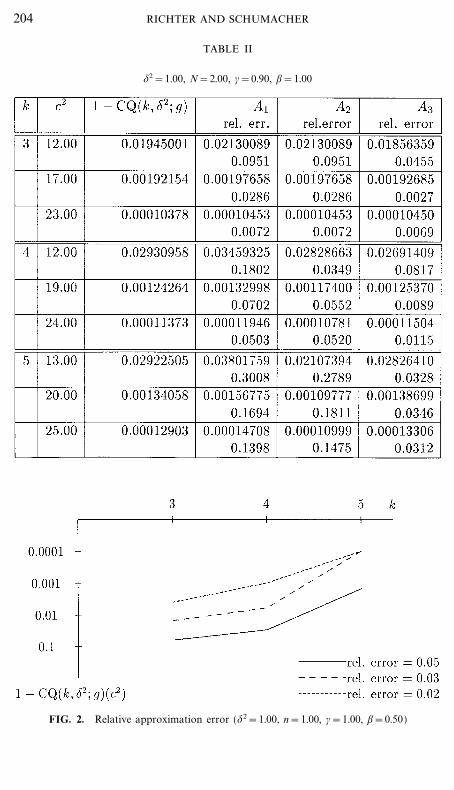
TABLE II

$2=1.00, N=2.00, #=0.90, ;=1.00

FIG. 2. Relative approximation error ($2=1.00, n=1.00, #=1.00, ;=0.50)


least-favorable parameter situations. Explicit approximation formulae aresometimes used in exact numerical methods for generating certain initialvalues. The explicit asymptotic approximations for large deviationprobabilities from Theorem 3.5 and Corollary 3.6 are used in Ittrich et al.(2000) for deriving more or less explicit asymptotic quantile approximationformulae and iteration procedures.

In the tables of this section we compare exact tail probabilities withapproximations for them based on the results of Corollary 3.6. To this endwe take into account approximation results using one, two, and three termsof the asymptotic expansion in the columns A1 , A2 , and A3 , respectively.In the evaluation of the leading term of the expansion we actually used b1

instead of the asymptotically equal term 1�(2$(k&1)�2(#;) (k+1)�2), becausethis proved to lead to more accurate approximations. The exact tailprobabilities in the column 1&CQ(k, $2; g) are determined using anumerical algorithm given in Ittrich et al. (2000).

Table I gives numerical results for the usual noncentral chi-square dis-tribution, whereas Table II deals with the noncentral generalized chi-squaredistribution when the density-generating function is of Kotz type with con-stants (N; #; ;)=(2; 0.9; 1).

These parameter configurations are chosen to reflect a certain typicalbehavior of the approximations.

Both tables show the decrease of relative error for increasing values of c.The approximation with two terms is not always superior to the one-termapproximation. Furthermore, the approximation becomes worse forincreasing dimension (d.f.). This indicates that an asymptotic expansionincluding additionally the asymptotic for k � � might result in betternumerical approximations for larger k.

Figure 2 illustrates how the degree of freedom k influence the values1&CQ(k, $2; g)(c2) for which relative approximation errors of 0.05, 0.03,and 0.02, respectively, can be guaranteed.

5. PROOFS AND AUXILIARY RESULTS

For y� y0 it holds that

F \A$c ,�g~ &1 \*

cy+ g~ ((c&$)2)+

c2 +=|k&1

|k|

arctan '( y)

0(sin :)k&2 d:


with

'( y)=�4$2g~ &1 \*

cy+ g~ ((c&$)2)+

\c2&$2& g~ &1 \*c

y+ g~ ((c&$)2)++2&1.

For proving Lemma 3.2 we start by expanding '( y) for y � 0.

Lemma 5.1. Under assumptions (D1) and (D2, m) it holds that

'( y)= :m&1

j=0

aj+1 y j+1�2+O( ym+1�2) (21)

as y � 0, where the first coefficients are

a1 =- c1

1

- $ (1&$�2),

a2=c3�21

3+$�c8$3�2(1&$�c)2+

c2

- c1

1

2 - $ c(1&$�c),

and

a3 =c5�21

23+10$�c&$2�c2

128$5�2(1&$�c)3 +- c1 c2

3(3+$�c)16$3�2c(1&$�c)2

&c2

2

c3�21

1

8 - $ c2(1&$�c)+

c3

- c1

1

2 - $ c2(1&$�c).

Proof. We start with considering

4$2g~ &1 \*c

y+ g~ ((c&$)2)+\c2&$2& g~ &1 \*

cy+ g~ ((c&$)2)++

2

=4$2

c2

g~ &1 \*c

y+ g~ ((c&$)2)+<c2

\1&$2

c2&g~ &1( *

c y+ g~ ((c&$)2))c2 +

2 .


From (D2, m) we have

4$2

c2

g~ &1 \*c

y+ g~ ((c&$)2)+<c2

\1&$2

c2&g~ &1( *

c y+ g~ ((c&$)2))c2 +

2

=4$2

c2

:m

j=0

cj \yc+

j

+O \\yc+

m+1

+_1&

$2

c2& :m

j=0

cj \yc+

j

+\\yc+

m+1

+&2

=1

\1&$c+

2

:m

j=0

cj \yc+

j

+O \\yc+

m+1

+_1&

12$(1&$�c)

:m

j=1

cjy j

c j&1+O \ym+1

cm +&2 .

Since

1(1&x)2= :

�

j=0

( j+1) x j for |x|<1,

we obtain for sufficiently large c and small y,

4$2g~ &1 \*c

y+ g~ ((c&$)2)+\c2&$2& g~ &1 \*

cy+ g~ ((c&$)2)++

=1

\1&$c+

2 _ :m

j=0

cj \yc+

j

+O \\yc+

m+1

+&

__ :m

j=0

( j+1) \ 12$(1&$�c)

:m

l=1

clyl

cl&1+j

+O( ym+1)&=

1

\1&$c+

2 _ :m

j=0

cj \yc+

j

+O \\yc+

m+1

+&_ :m

j=0

A� j y j+O( ym+1)& ,


where

A� 0 =1,

A� 1=c1

$(1&$�c),

A� 2=3c2

1

4$2(1&$�c)2+c&2

c$(1&$�c),

A� 3=c3

1

2$3(1&$�c)3+3c1c2

2c$2(1&$�c)2+c3

c2$(1&$�c),

and

A� j=A� j (c, *)=O(1) as c � �, j=4, ..., m.

This leads to

4$2g~ &1 \*c

y+g~ ((c&$)2)+\c2&$2&g~ &1 \*

cy+g~ ((c&$)2)++

2= :m

j=0

Aj y j+O(ym+1), y � 0,

with

A0 =1,

A1=c1

$(1&$�c)2 ,

A2=c21

3+$�c4$2(1&$�c)3+c2

1c$(1&$�c)2 ,

A3=c3

1(2+$�c)4$3(1&$�c)

+c1c2(3+$�c)2c$2(1&$�c)3+

c3

c2$(1&$�c)2 ,

and

Aj=Aj (c, *)=O(1), c � �, j=4, ..., m.

We are now able to expand '. It is

'( y)=� :m

j=1

Aj y j+O( ym+1), y � 0,

=- A1 y1�2 �1+ :m

j=2

Aj

A1

y j&1+O( ym), y � 0.


Using

- 1+x= :m&1

j=0

&j x j+O(xm), |x|<1,

we get for sufficiently small y that

'( y)=- A1 y1�2 _ :m&1

j=0

&j _ :m

l=2

Al

A1

yl&1&j

+O( ym)& .

The proof of the lemma is finished by rearranging the terms in bracketsaccording to the ascending powers of y. K

We now put

'~ ( y)='( y2)

and consider

9k( y)=|arctan '~ ( y)

0(sin :)k&2 d:. (22)

Note that

F \A$c ,�g~ &1 \*

cy+ g~ ((c&$)2)+

c2 +=|k&1

|k9k(- y). (23)

It follows that

9$k( y)='~ ( y)k&2 '~ $( y)[1+'~ 2( y)]k�2 . (24)

This representation enables us to derive an expansion for 9k by firstexpanding 9$k using Lemma 5.1 and then applying termwise integration.

Proof of Lemma 3.2. Using the continuous differentiability of ', from(21) one can derive an expansion for '~ $,

'~ $( y)= :m&1

j=0

aj+1 y2 j (2 j+1)+O( y2m).


Inserting this expansion, together with (21), into the relation (24) gives

9$k( y)

=[�m&1

j=0 a j+1 y2 j+1+O( y2m+1)]k&2 [�m&1j=0 a j+1 y2 j (2 j+1)+O( y2m)]

[1+[�m&1j=0 aj+1 y2 j+1+O( y2m+1)]2]k�2 .

(25)

It holds that

_ :m&1

j=0

aj+1 y2 j+1+O( y2m+1)&k&2

=ak&21 yk&2 _ :

m&1

j=0

+ j y2 j+O( y2m)& , (26)

where

+0 =1,

+1=(k&2)a2

a1

,

+2=(k&2)a3

a1

+(k&2)(k&3)

2a2

2

a21

,

and

+j=+j (*, c)=0(1), c � �, j=3, ..., m&1.

Furthermore, we have

_1+_ :m&1

j=0

a j+1 y2 j+1+O( y2m+1)&2

&k�2

= :m&1

l=0\k�2

l +\ :m&1

j=0

aj+1 y2 j+1+2l

+O( y2m)

=1+ :m&1

j=1

&j y2 j+O( y2m)

with

&1 =k2

a21 ,

&2=ka1 a2+k(k&2)

8a4

1 ,


and

&j=&j (*, c)=0(1), c � �, j=3, ..., m&1.

Because of

11+x

= :m&1

l=0

(&1) l x l+O(xm), |x|<1,

this leads to

1[1+'~ 2( y)]k�2= :

m&1

j=0

!j y2 j+O( y2m), y � 0, (27)

with

!0 =1,

!1= &k2

a21 ,

!2= &ka1a2+k(k+2)

8a4

1 ,

and

!j=!j (*, c)=O(1), c � �, j=3, ..., m&1.

Combining (25), (26), and (27) yields:

9$k( y)=ak&21 yk&2 _ :

m&1

j=0

+j y2 j+O( y2m)&__ :

m&1

j=0

a j+1 y2 j (2 j+1)+O( y2m)&_ :m&1

j=0

! j y2 j+O( y2m)&= :

m&1

j=0

Bj yk&2+2 j+O( yk&2+2m),


with

B0 =ak&11 ,

B1= &k2

ak+11 +(k+1) ak&2

1 a2 ,(28)

B2=ak&21 a3(k+3)+

(k&2)(k+3)2

ak&31 a2

2

&k(k+3)

2ak

1 a2+k(k+2)

8ak+3

1 ,

and

Bj=Bj (*, c)=O(1), c � �, j=3, ..., m&1.

Termwise integrating this relation with respect to y and inserting the result-ing expansion into (23) completes the proof. K

Proof of Lemma 3.3. To expand fk we insert the expansion of the inter-section-percentage function and that from assumption (D2, m) into therelation

fk(c, *, y)=F \A$c ,�g~ &1 \*

cy+ g~ ((c&$)2)+

c2 +__g~ &1 \*

cy+ g~ ((c&$)2)+&

(k&2)�2

g~ &1$ \*c

y+ g~ ((c&$)2)+ .

This yields

fk(c, *, y)=|k&1

|k

ck+1

* _ :m&1

j=0

B j

k&1+2 jy(k&1)�2+ j+O( y(k&1)�2+m)&

__ :m

j=0

cj \yc+

j

+O \\yc+

m+1

+&(k&2)�2

__ :m

j=1

cj jy j&1

c j +O \ ym

cm+1+& .


We again make use of the binomial expansion

_ :m

j=0

cj \yc+

j

+O \\yc+

m+1

+&(k&2)�2

=c(k&2)�2o _ :

m

j=0

*j \yc+

j

+O \\yc+

m+1

+&with

*0 =1,

*1=(k&2) c1

2c0

,

*2=(k&2) c2

2c0

+(k&2)(k&4) c2

1

8c20

,

and

*j=*j (c, *)=O(1), c � �.

This finally gives

fk(c, *, y)=|k&1

|k

ck+1

* \ :m&1

j=0

B j

k&1+2 jy(k&1)�2+ j+O( y(k&1)�2+m)+

_c (k&2)�20 _ :

m

j=0

*j \yc+

j

+O \\yc+

m+1

+&__ :

m

j=1

cj jy j&1

c j +O \ ym

cm+1+&=

|k&1

|k

ck

*:

m&1

j=0

bj+1 y(k&1)�2+ j+O( y(k&1)�2+m)

with

b1 =c (k+1)�2

1

(k&1) $(k&1)�2(1&$�c),

b2=c (k+3)�2

1

$(k+1)�2(1&$�c)3 _&k&3

8(k+1)+

k&34(k&1)

$c

&$2

8c2&+

c (k&1)�21 c2

c$(k&1)�2(1&$�c)k+3

2(k&1),


and

b3 =c (k+5)�2

1

$(k+3)�2(1&$�c)5 _(k&5)(k&3)128(k+3)

&(k&5)(k&3)

32(k+1)$c

+3(k&5)(k&3)

64(k&1)$2

c2&k&5

32$3

c3+k&3128

$4

c4&+

c (k+1)�21 c2

c$(k+1)�2(1&$�c)3 _(k+5)(k&3)16(k+1)

&(k+5)(k&3)

8(k&1)$c

+k+5

16$2

c2&+

c (k&1)�21 c3

c2$(k&1)�2(1&$�c)k+5

2(k&1)+

c (k&3)�21 c2

2

c2$(k&1)�2(1&$�c)k+5

8. K

Proof of Corollary 3.6. From Example 2 we know that the Kotz typedensity-generating function satisfies the assumption (D2, m) with *=c2#.Thus for #> 1

2 the assumptions of Theorem 3.5 are fulfilled. Furthermore,

Ik, g~ =1 \2N+k&2

2# +2#;(2N+k&2)�(2#) .

To obtain the coefficients of the asymptotic expansion we evaluate

b1(k&1)2

=c (k+1)�2

1

2$(k&1)�2(1&$�c)

=(1&$�c)k

2$(k&1)�2 \#;(1&$�c)2#&N&1

c2# +(k+1)�2 ,

b2(k&1)(k+1)4

=&c (k+3)�2

1 (k&1)(k&3)32$(k+1)�2(1&$�c)3 +

c (k+3)�21 (k+1)(k&3)

16c$(k&1)�2(1&$�c)3

&c (k+3)�2

1 (k&1)(k+1)32c2$(k&3)�2(1&$�c)3+

c (k&1)�21 c2(k+3)(k+1)

8c$(k&1)�2(1&$�c),

and

b3

(k&1)(k+1)(k+3)8

=c (k+5)�2

1 (k&5)(k&3)(k&1)(k+1)

1024$(k+3)�2 \1&$c+

5

&c (k+5)�2

1 (k&5)(k&3)(k&1)(k+3)

256c$(k+1)�2 \1&$c+

5


+3c(k+5)�2

1 (k&5)(k&3)(k+1)(k+3)

512c2$(k&1)�2 \1&$c+

5

&c (k+5)

1 (k&5)(k&1)(k+1)(k+3)

256c3$(k&3)�2 \1&$c+

5

+c (k+5)�2

1 (k&3)(k&1)(k+1)(k+3)

1024c4$(k&5)�2 \1&$c+

5

+c (k+1)�2

1 c2(k&3)(k&1)(k+3)(k+5)

128c$(k+1)�2 \1&$c+

3

&c (k+1)�2

1 c2(k&3)(k+1)(k+3)(k+5)

64c2$(k&1)�2 \1&$c+

3

+c (k+1)�2

1 c2(k&1)(k+1)(k+3)(k+5)

128c3$(k&3)�2 \1&$c+

3

+c (k&1)�2

1 c3(k+1)(k+3)(k+5)

16c2$(k&1)�2 \1&$c+

+c (k&3)�2

1 c22(k&1)(k+1)(k+3)(k+5)

64c2$(k&1)�2 \1&$c+

.

Rearranging the terms according to powers of c, putting the leading termoutside the brackets, and using

b1 t1

(k&1) $(k&1)�2(#;) (k+1)�2 , c � �,


lead to expansion (20), where

D1&2# = &c (k+3)�2

1

b1$(k+1)�2 \1&$c+

3

k&316

D&2#=c (k+3)�2

1

b1$(k&1)�2 \1&$c+

3

(k+1)(k&3)8(k&1)

+c(k&1)�2

1 c2

b1$(k&1)�2 \1&$c+

(k+1)(k+3)4(k&1)

D&1&2#= &c (k+3)�2

1

b1$(k&3)�2 \1&$c+

3

k+116

D2&4#=c (k+5)�2

1

b1$(k+3)�2 \1&$c+

5

(k&5)(k&3)(k+1)512

D1&4#= &c (k+5)�2

1

b1$(k+1)�2 \1&$c+

5

(k&5)(k&3)(k+3)128

+c(k+1)�2

1 c2

b1 $(k+1)�2 \1&$c+

3

(k&3)(k+3)(k+5)64

D&4#=c (k+5)�2

1

b1$(k&1)�2 \1&$c+

5

3(k&5)(k&3)(k+1)(k+3)256(k&1)

&c (k+1)�2

1 c2

b1$ (k&1)�2 \1&$c+

3

(k&3)(k+1)(k+3)(k+5)32(k&1)

+c (k&1)�2

1 c3

b1$(k&1)�2 \1&$c+

(k+1)(k+3)(k+5)8(k&1)

+c (k&3)�2

1 c22

b1$ (k&1)�2 \1&$c+

(k+1)(k+3)(k+5)32


D&1&4#= &c (k+5)�2

1

b1$(k&3)�2 \1&$c+

5

(k&5)(k+1)(k+3)128

+c(k+1)�2

1 c2

b1 $(k&3)�2 \1&$c+

3

(k+1)(k+3)(k+5)64

D&2&4#=c (k+5)�2

1

b1$(k&5)�2 \1&$c+

5

(k&3)(k+1)(k+3)512

,

where

b1=\1&

$c+

k

(k&1) $(k&1)�2 \#; \1&$c+

2#

&N&1

c2# +(k+1)�2

and the coefficients cj , j=1, 2, 3, are given in Example 2. K

ACKNOWLEDGMENT

The authors thank K. Breitung for a useful discussion and the referees for their constructivecriticisms of this paper which influenced its final presentation.

REFERENCES

1. T. W. Anderson and K. T. Fang, Tech. Rep. 53, Department of Statistics, StanfordUniversity, Stanford, CA, 1982.

2. N. Bleistein and R. A. Handelsman, `Àsymptotic Expansions of Integrals,'' Holt,Rinehart, and Winston, New York, 1975.

3. K. Breitung and W.-D. Richter, A geometric approach to an asymptotic expansion forlarge deviation probabilities of Gaussian random vectors, J. Multivariate Anal. 58 (1996),1�20.

4. T. Cacoullous and M. Koutras, Quadratic forms in spherical random variables:generalized noncentral /2 distribution, Naval Res. Logistics Quart. 31, No. 3 (1984),447�461.

5. H. E. Daniels, Tail probability approximations, Internat. Statist. Rev. 55 (1987), 37�48.6. A. S. S. Dorflo, A unified method for computing probabilities of misclassification when the

covariance matrices are known, Comm. Statist. Simula. 22, No. 3 (1993), 679�687.7. M. V. Fedorjuk, ``Saddlepoint Method,'' Nauka, Moscow, 1977. [In Russian]8. A. K. Gupta and T. Varga, `Èlliptically Contoured Models in Statistics,'' Kluwer

Academic, Dordrecht�Boston�London, 1993.


9. H. Hsu, Noncentral distributions of quadratic forms for elliptically contoured distribu-tions, in ``Statistical Inference in Elliptically Contoured and Related Distributions''(K. T. Fang and T. W. Anderson, Eds.), pp. 97�102, Allerton Press, New York, 1990.

10. C. Ittrich, D. Krause, and W.-D. Richter, Probabilities and large quantiles of noncentralgeneralized chisquare distributions, Statistics 34 (2000), 53�101.

11. D. Kelker, Distribution theory of spherical distributions and a location-scale parametergeneralization, Sankhya A 32 (1970), 419�430.

12. W.-D. Richter, Eine geometrische Methode in der Stochastik, Rostock Math. Kolloq. 44(1991), 63�72.

13. W.-D. Richter, Eine geometrische und eine asymptotische Methode in der Statistik,preprint, Universita� t Bremen, 1992.

14. W.-D. Richter, A geometric approach to the Gaussian law, in ``Symposia Gaussiana,Conference B'' (Mammitzsch and Schneewei?, Eds.), pp. 25�45, de Gruyter, Berlin�NewYork, 1995.

15. W.-D. Richter and J. Schumacher, Laplace method in large deviation theory, Rost. Math.Koll. 44 (1990), 47�52.

16. I. J. Schoenberg, Metric spaces and completely monotone functions, Ann. Math. 39(1938), 811�841.

17. R. Wong, `Àsymptotic Approximations of Integrals,'' Academic Press, Boston, 1989.


Documents

Asymptotic Expansions for Large Deviation Probabilities of Noncentral …richter/W-DR2000-1.pdf · 2012-03-27 · Asymptotic Expansions for Large Deviation Probabilities ... generalized