Testing Structural Stability With Endogenous Break Point:A Size Comparison of Analytic and Bootstrap Procedures

Francis X. Diebold and Celia Chen

September 1992Revised, July 1993

This Print: September 25, 1996

Department of EconomicsUniversity of Pennsylvania

3718 Locust WalkPhiladelphia, PA 19104-6297

(Address all correspondence to Diebold.)JEL Classification: C12, C15, C22Keywords: Structural change, bootstrap

Abstract: We compare the performance of two alternative approximations to the finite-sampledistributions of test statistics for structural change, one based on asymptotics and one basedon the bootstrap. We focus on tests acknowledging that the break point is selectedendogenously--in particular, the "supremum" tests of Andrews (1993). We explore a varietyof issues of interest in applied work, focusing particularly on smaller samples and persistentdynamics. The bootstrap approximation to the finite-sample distribution appears consistentlyaccurate, in contrast to the asymptotic approximation. The results are of interest not onlyfrom the perspective of testing for structural change, but also from the broader perspective ofcompiling evidence on the adequacy of bootstrap approximations to finite-sampledistributions in econometrics.

Acknowledgements: We are grateful to three referees for their constructive comments. Manycolleagues provided helpful comments as well; special thanks go to Don Andrews, Jean-Marie Dufour, Neil Ericsson, Eric Ghysels, Walter Krämer, and Jim Stock, as well as seminarparticipants at the Montreal/C.R.D.E. Conference on the Econometrics of Structural Change,Penn, SUNY Albany, Indiana, Illinois, Ohio State, the Federal Reserve Bank of Kansas City,and the Federal Reserve Board. We alone are to blame for remaining shortcomings. Wegratefully acknowledge the support of the National Science Foundation, the SloanFoundation, and the University of Pennsylvania Research Foundation.

Chow (1986) and Hackl and Westlund (1989) provide useful surveys.1

1

1. Introduction

Structural change is of paramount importance in economics and econometrics, and the

associated literature is huge. An important associated problem is testing the null hypothesis1

of structural stability against the alternative of a one-time structural break. In standard

treatments, the location of the potential break is assumed known a priori. The standard

approach is often highly unrealistic, however, because of the endogeneity, or sample

selection, problem. That is, implicitly or explicitly, data-based procedures are typically used

to determine the most likely location of a break, thereby invalidating the distribution theory

associated with conventional tests.

Tests formally incorporating selection effects are therefore desirable. Important such

tests are the "supremum" test of Andrews (1993) and the related "average" and "exponential"

tests of Andrews and Ploberger (1992), Andrews, Lee, and Ploberger (1992) and Hansen

(1991a, 1991b). At issue, however, is how best to approximate their finite-sample

distributions under the null hypothesis of structural stability.

One obvious approximation to the finite-sample distribution is the asymptotic

distribution obtained by Andrews (1993). The asymptotic distribution is relatively easy to

characterize and tabulate, but it may be an unreliable guide to finite-sample behavior. An

alternative approximation is the bootstrap distribution, as suggested by Christiano (1992).

Bootstrap procedures play upon the increased sophistication and feasibility of simulation

methods in econometrics, together with drastic increases in computing capability. Bootstrap

methods are typically employed in hopes of obtaining better approximations to finite-sample

yt yt 1 t , t 1, ..., T

t N(0,1)

We also examined a variety of leptokurtic and skewed innovations, against which all of2

our results were robust.

2

distributions, but as of now the theory is far from complete, and the efficacy of the bootstrap

in this application remains an open question.

In this paper, we provide a detailed finite-sample evaluation of the size of supremum

tests for structural change in a dynamic model, with attention focused on the comparative

performance of asymptotic vs. bootstrap procedures. In doing so, we build upon and extend

both Andrews' and Christiano's work. The results are of interest not only from the perspective

of testing for structural change, but also from the broader perspective of compiling evidence

on the adequacy of bootstrap approximations to finite-sample distributions in econometrics.

In section 2, we introduce the basic model and test statistics. The heart of the paper is section

3, in which we execute the test size comparison and present the results in both tabular and

graphical (response surface) form. In section 4, we extend the analysis to include richer data-

generating processes and alternative test statistics. We conclude and sketch directions for

future research in section 5.

2. The Basic Model and Tests

Here we discuss our most basic model and test statistics, which are the centerpiece of

the analysis. We work with the Gaussian zero-mean first-order autoregressive process,2

y0 N 0, 11 2

< 1.

yt yt 1 t , t 1, ..., T.

yt 1 yt 1 t , t 1, ..., T

yt 2 yt 1 t , t (T 1), ..., T.

SupW max Tˆ ˆ ˆ

1ˆ

1ˆ

2ˆ

2

ˆ1ˆ

1ˆ

2ˆ

2

SupLM max Tˆ ˆ ˆ

1ˆ

1ˆ

2ˆ

2

ˆ ˆ

3

The null hypothesis of structural stability is

We call this the restricted, or no-break, model. The alternative hypothesis of a one-time

structural break is

We call these the unrestricted, or subsample, models.

Our basic test statistics are the "supremum" tests of Andrews (1993),

SupLR max T logˆ ˆ

ˆ1ˆ

1ˆ

2ˆ

2,

ˆ ˆ1

ˆ2

[.15, .85].

We could, of course, trim by other amounts. The bootstrap procedure that we introduce3

can be easily modified to do so. But Andrews tabulated only the asymptotic distribution for [.15, .85]. So, to maintain comparability, we follow suit.

4

where is the Tx1 vector of OLS residuals from the restricted model, is the T x1 vector*

of OLS residuals from the subsample 1 model, is the (T-T )x1 vector of OLS residuals*

from the subsample 2 model, and = T /T. Following standard procedure, we*

impose 3

We consider two ways of approximating the finite-sample distributions of the three

statistics (that is, ways of approximating the significance level, or p-value, corresponding to a

given value of a test statistic). The first approximation is Andrews' (1993) asymptotic

distribution, which is essentially the distribution of the supremum of a set of random2

variables. This is obviously appropriate asymptotically, although little is known about the

reliability of the asymptotic distribution as a guide to finite-sample behavior. Andrews'

Monte Carlo analysis indicates that the asymptotic approximation performs quite well;

however, he examines only a restrictive static regression model with a single deterministic

regressor. In contrast, we focus on dynamic models.

The second approximation is the bootstrap distribution. Bootstrapping was first

applied to the endogenous change-point problem by Christiano (1992), who used the

Our procedure is a "nonparametric bootstrap," by virtue of the fact that no distributional4

assumptions are made. If distributional information is available, one may of course draw thepseudo-disturbances from the appropriate parametric distribution fitted to the model residuals,resulting in a "parametric bootstrap". In practice, the nonparametric bootstrap is morepopular, as one is usually unsure of the underlying density.

5

supremum of Chow's (1960) F test to assess the likelihood of a structural shift in the dynamics

of U.S. aggregate output. Our bootstrap procedures are straightforward generalizations of his

to a richer class of tests.

The bootstrap formalizes a highly intuitive idea. Using observed data, we calculate the

test statistic of interest. Then we build up an approximation to its finite-sample null

distribution by (1) generating many pseudo-data samples using model parameters estimated

under the null hypothesis and pseudo-disturbances drawn with replacement from the

estimated model's residuals, and then (2) calculating the statistic for each sample of pseudo-

data. We call this the "bootstrap distribution". Finally, we compute the approximate p-value4

as the probability, relative to the bootstrap distribution, of obtaining a larger value of the test

statistic than the one actually obtained.

The results of Gené and Zinn (1990) and Stinchcombe and White (1993) show that

the bootstrap procedures we use in this paper are asymptotically valid. The finite-sample

properties of the bootstrap, however, are much less well understood. Recent research shows

that in many cases, roughly speaking, the bootstrap is similar to a two-term empirical

Edgeworth expansion, although in some important cases it can be shown to be even better

(e.g., Bhattacharya and Qumsiyeh, 1989, and Hall, 1992). At the very least, the likely

impressive finite-sample performance of the bootstrap has emerged as an empirical "folk

theorem," supported by various Monte Carlo studies. (See, for example, the insightful survey

2(1)

ˆ 0 S/RM,

6

of Jeong and Maddala, 1992.)

Having sketched the basic model and test statistics, we now proceed to the finite-

sample comparisons of test size.

3. Monte Carlo Analysis of Test Size

First let us define some notation. ChiSupW, ChiSupLR, and ChiSupLM refer to tests

against the distribution. AsySupW, AsySupLR, and AsySupLM refer to tests against

Andrews' (1993) asymptotic distribution. BootSupW, BootSupLR, and BootSupLM refer to

tests against the bootstrap distribution.

For each procedure, we explore the relationship between empirical and nominal test

size, varying the sample size (T), persistence as measured by the autoregressive coefficient

( ), and nominal test size ( ). We explore sample sizes of T = 10, 50, 100, 500, 1000,

persistence parameters of = .01, .20, .30, .40, .50, .60, .70, .80, .83, .85, .87, .90, .92, 95,

.96, .97, .98, .99, and nominal test sizes of = 1%, 2.5%, 5%, and 10%. We perform RM =

1000 Monte Carlo replications. Given the choices of T, , and , we use a full factorial

experimental design for examining the properties of the AsySup tests, and a subset of the full

factorial design for examining the ChiSup and BootSup tests.

We seek to estimate the probability of rejecting the hypothesis of structural stability

when it is true (for a fixed nominal test size ), for each of the test procedures outlined above,

and to see how those probabilities vary with T, and . Let the true, or empirical, test size be

denoted by . Following standard practice, we use the unbiased and asymptotically (in RM)0

normal estimator where S is the total number of times

ˆ 0 ( 0(1 0)/RM)½

( ˆ 0(1 ˆ 0)/RM)½

ˆ 0 ,

ˆ 0 ˆ 0,

The response surfaces were also estimated separately for each nominal size. The R 's for5 2

those regressions were of course a bit higher than for the surfaces reported here. The actualgraphs of the separately estimated surfaces, however, are virtually identical to those of thesurfaces reported here, all of which still have very high R . 2

7

the procedure rejects. The asymptotic (in RM) standard error of is

which we estimate by

In addition to presenting the actual Monte Carlo test-size results for each

approximation to the finite-sample distribution, we summarize the results succinctly by

estimating response surfaces, as advocated by Hendry (1984) and Ericsson (1991). To fit a

response surface, we use data from all relevant Monte Carlo experiments to determine how

the size distortion, depends on T, , and . Typically, we start with a second-order

expansion in powers of T , and , as well as terms capturing interaction of and with T. -1/2

We then obtain the final response-surface specifications by dropping variables with

insignificant t-ratios. Because the variance of varies with the value of the t-ratios

are constructed using White's (1980) heteroskedasticity-consistent standard errors. The final

specifications of the response surfaces are given in Table 1.5

All computations were done using 386-MATLAB version 3.5k on an IBM-compatible

486 machine running at 33 MHz. All N(0,1) deviates were generated using the Forsythe et al.

(1977) algorithm, as implemented in MATLAB, and all U(0,1) deviates were generated using

the Park-Miller (1988) algorithm, also as implemented in MATLAB.

Results for ChiSupW, ChiSupLR, ChiSupLM

As is now well known, the distribution does not obtain, even asymptotically,2

ˆ 0 ,

The response surfaces for ChiSupLR and ChiSupLM are similar to that of ChiSupW and6

therefore are not included here.

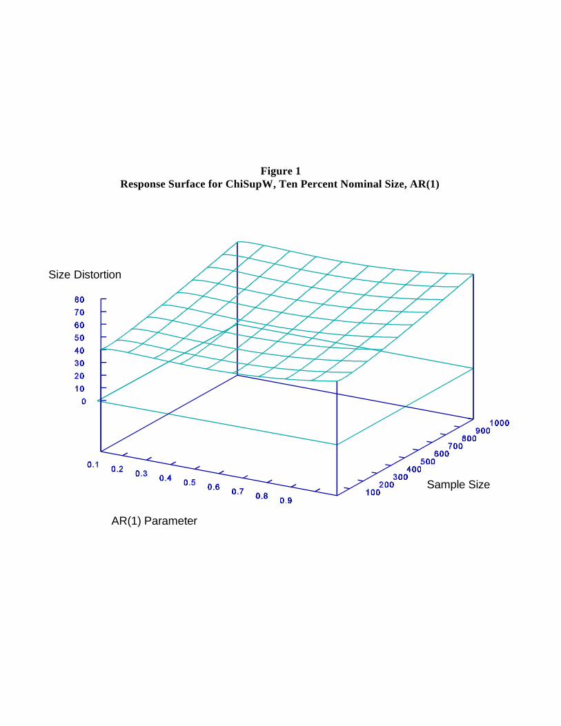
We superimpose graphs of the x-y plane on most of our graphs of response surfaces. A7

response surface that lies near the x-y plane indicates that the distribution approximates thefinite sample distribution well. Clearly, this is not the case for the ChiSup tests.

Hence T appears in positive rather than negative powers in the response surface.8

8

because the location of the break point is selected with the aid of the data. Nevertheless, the

use of such approximations remains commonplace in applied work. Examination of the

finite-sample properties of the ChiSup tests illustrates the severity of the size distortions and

provides a key benchmark against which to compare the results for other tests.

The Monte Carlo experiments using the distribution use the T and values2

described above, and persistence parameters of = .01, .50, .70, .80, .83, .85, .87, .90, .92,

.95, .96, .97, .98, .99. To save space, we present in Table 2 the results from only a small but

representative subset of the parameter space points actually explored. As intuition suggests,

the ChiSup tests tend to overreject. Moreover, the size distortions are huge. For example,

the response surface for ChiSupW (Figure 1), which plots the size distortion, as a

function of sample size and persistence when nominal test size is fixed at 10%, highlights

their poor performance: empirical test size typically dwarfs nominal test size. 6, 7

Furthermore, the tendency for the ChiSup tests to overreject worsens as sample size increases,

due to the increased severity of data mining. Serial correlation also affects the empirical size8

of the ChiSup tests. As the degree of serial correlation increases, the ChiSup tests tend to

reject more often. The extent to which the tests overreject from using the incorrect asymptotic

distribution, however, far overpowers this effect.

ˆ 0 ,

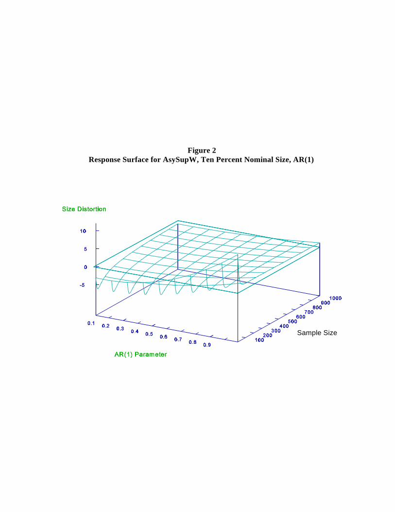
Note the scale change of the z axis relative to Figure 1.9

9

Results for AsySupW, AsySupLR, AsySupLM

Having seen how poorly the distribution performs as an approximation to the finite-2

sample distribution, we now turn to the asymptotic approximation. The full factorial

experimental design is used here, although again we present only a subset of the results, this

time in Table 3 and Figures 2-4. The basic observations are:9

(i) Use of the asymptotic distribution yields large reductions in size distortion relative

to use of the distribution. Significant distortions remain, however.2

(ii) Clearly, and as expected, nominal and empirical test size converge as T grows.

(iii) Table 3 confirms that the expected relationship, SupW SupLR SupLM, holds

throughout. (This must hold at any break point, and therefore for the

supremum.) In line with this, for small samples, AsySupW tends to overreject,

AsySupLR to underreject and AsySupLM to underreject drastically.

(iv) The response surfaces in Figures 2-4 show that the size distortion, is

generally large (and negative) for small T, and decreases with T. The

convergence of empirical to nominal test size, however, can be slow and non-

monotone, particularly with the amounts of serial correlation typically present

in economic data.

(v) Serial correlation tends to inflate empirical test size. The stronger the serial

correlation, the greater the empirical size inflation. Additionally, for AsySupW

and AsySupLR the sensitivity to serial correlation is greater the smaller the

sample size. This can be seen most clearly for the case of AsySupW where the

Throughout, we set RB = 1000.10

10

values for T = 10 are larger than for T= 100.

(vi) The size distortions associated with the AsySupLM procedure in small samples

are particularly severe.

Let us elaborate upon points (iv) and (v). It is important to note that there are

effectively two sources of test size distortion. First, in the absence of serial correlation, finite-

sample empirical test size tends to be pushed downward relative to nominal size. Serial

correlation works in the opposite direction, pushing empirical test size upward. Thus, the

occasional good test size performance is merely an artifact of a happenstance cancellation of

competing biases, and should never be relied upon to work in practice.

The upshot of this subsection is that, although the finite-sample performance of the

AsySup statistics is much better than that of the ChiSup statistics, it is not as good as one

would hope. Whether there exists an even better approximation to the finite-sample

distribution--one that corrects the deficiencies of the asymptotic distribution--remains an open

question. This leads us to the bootstrap procedure, to which we now turn.

Results for BootSupW, BootSupLR, BootSupLM

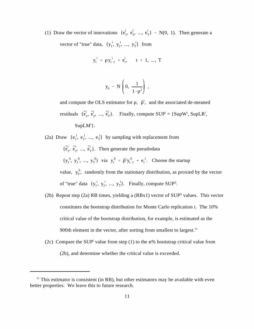
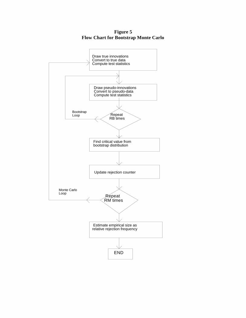
We provide a flow chart illustrating our Monte Carlo procedure for evaluating the

bootstrap in Figure 5. The details of the procedure, and our Monte Carlo examination of its

properties, are as follows. Let i = 1, ..., RM index Monte Carlo replications, and let j = 1, ...,

RB index the bootstrap replications inside each Monte Carlo replication. Nominal test size10

is . Then:

y it y i

t 1it , t 1, ..., T

y0 N 0, 11 2

,

{ i1,

i2, ..., i

T} N(0, 1).

{y i1 , y i

2 , ..., y iT}

ˆ i,

{ˆ i1, ˆ i

2, ..., ˆ iT}.

{e j1 , e j

2 , ..., e jT}

{ˆ i1, ˆ i

2, ..., ˆ iT}.

{y ij1 , y ij

2 , ..., y ijT } y ij

t ˆ iy ijt 1 e j

t .

y ij0 ,

{y i1 , y i

2 , ..., y iT}.

This estimator is consistent (in RB), but other estimators may be available with even11

better properties. We leave this to future research.

11

(1) Draw the vector of innovations Then generate a

vector of "true" data, from

and compute the OLS estimator for , and the associated de-meaned

residuals Finally, compute SUP = {SupW , SupLR , i i i

SupLM }.i

(2a) Draw by sampling with replacement from

Then generate the pseudodata

via Choose the startup

value, randomly from the stationary distribution, as proxied by the vector

of "true" data Finally, compute SUP .ij

(2b) Repeat step (2a) RB times, yielding a (RBx1) vector of SUP values. This vectorij

constitutes the bootstrap distribution for Monte Carlo replication i. The 10%

critical value of the bootstrap distribution, for example, is estimated as the

900th element in the vector, after sorting from smallest to largest.11

(2c) Compare the SUP value from step (1) to the % bootstrap critical value fromi

(2b), and determine whether the critical value is exceeded.

LR T log(1 WT

) T log 1ˆ ˆ ˆ

1ˆ

1ˆ

2ˆ

2

ˆ1ˆ

1ˆ

2ˆ

2

T logˆ ˆ

ˆ1ˆ

1ˆ

2ˆ

2

LM W

1 WT

Tˆ ˆ ˆ

1ˆ

1ˆ

2ˆ

2

ˆ1ˆ

1ˆ

2ˆ

2

ˆ ˆ

ˆ1ˆ

1ˆ

2ˆ

2

Tˆ ˆ ˆ

1ˆ

1ˆ

2ˆ

2

ˆ ˆ.

12

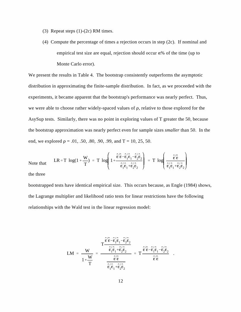
(3) Repeat steps (1)-(2c) RM times.

(4) Compute the percentage of times a rejection occurs in step (2c). If nominal and

empirical test size are equal, rejection should occur % of the time (up to

Monte Carlo error).

We present the results in Table 4. The bootstrap consistently outperforms the asymptotic

distribution in approximating the finite-sample distribution. In fact, as we proceeded with the

experiments, it became apparent that the bootstrap's performance was nearly perfect. Thus,

we were able to choose rather widely-spaced values of , relative to those explored for the

AsySup tests. Similarly, there was no point in exploring values of T greater the 50, because

the bootstrap approximation was nearly perfect even for sample sizes smaller than 50. In the

end, we explored = .01, .50, .80, .90, .99, and T = 10, 25, 50.

Note that

the three

bootstrapped tests have identical empirical size. This occurs because, as Engle (1984) shows,

the Lagrange multiplier and likelihood ratio tests for linear restrictions have the following

relationships with the Wald test in the linear regression model:

LRW

11 W/T

LMW

1(1 W/T)2

For that reason, the x-y plane is not graphed in Figure 6.12

13

Because the first derivatives, and are greater

than zero (so long as W > 0), LR and LM are monotone increasing functions of W. This

means that the break point that gives the SupW statistic will also be the break point that gives

the SupLR and SupLM statistics. If the "true" SupW is equal to the 900th largest SupW ofi ij

the bootstrap SupW distribution, then the "true" SupLR is equal to the 900th largest SupLRi i ij

in the bootstrapped finite-sample distribution for the SupLR test statistic, and similarly for the

SupLM test. Thus, the bootstrap distributions adjust for the differences among the SupW, LR

and LM statistics.

We also present the estimated response surface for the bootstrap in Figure 6. The

performance of the bootstrap is visually striking. As expected, it has little curvature;

effectively, it is just the plane containing the x and y axes. 12

The results demonstrate that the bootstrap distribution can be a much better

approximation to the finite-sample distribution than the asymptotic distribution when sample

size is not large and/or persistence is high. Note, in particular, that the finite-sample size

distortion associated with the use of bootstrapped critical values is minimal, regardless of the

value of the nuisance parameter . This stands in sharp contrast to the finite-sample size

distortion associated with the use of asymptotic critical values, which depends heavily on , in

spite of the fact that dependence on vanishes in the limit.

Moreover, our results are entirely in line with those of Rayner (1990), who finds that

the bootstrap approximation to the finite-sample distribution of studentized statistics in an

AR(1) model outperforms the asymptotic approximation for sample sizes as small as T=5 and

14

for degrees of persistence as large as =0.99. Jeong and Maddala (1992) suggest that one

reason for Rayner's success with the bootstrap is his careful treatment of the initial value when

generating bootstrap samples. Instead of assuming the initial value to be known, he draws it

from its stationary distribution. We of course followed the same approach.

We conclude this subsection with some discussion of the computational requirements

of the bootstrap. Although it is true that a Monte Carlo evaluation of the bootstrap is a

formidable computational task, actual use of the bootstrap on a real dataset is a simple matter.

For example, performing the BootSupLR test for a sample of size 50 takes about ten minutes

on a 33 MHz 486 machine.

4. Extensions to Other Models and Other Tests

Other Models

We now extend the analysis to richer models, by allowing for inclusion of an intercept.

For each AsySup test statistic, the experiments are over T = 10, 50, 100, 500, and = .01, .50,

.80, .99, while for the BootSup tests, the experiments are over T = 10, 25, 50, and = .01, .50,

.80, .90, .99. The size distortions of the AsySup tests can be extremely large when allowance

for intercept is made. For example, in Figure 7 we graph the response surface for the

AsySupW test when an intercept is included in the estimation. Comparing this against Figure

2, the zero-mean case, the basic shape of the response surfaces remains the same. But when a

ExpK log 1.85T .15T 1

exp( 12

K( ))

AvgK 1.85T .15T 1

K( ),

Again note the change in the scale of the z axis.13

Of course, as sample size grows and for moderate levels of serial correlation, the size14

distortion almost disappears, as is consistent with the asymptotic behavior of the tests.

15

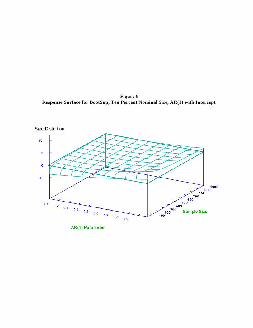
mean is included, the size distortions become much worse. In contrast, the bootstrap13 14

(Figure 8) appears to continue to deliver outstanding approximations to the null distributions

of the test statistics, with the response surface lying almost completely on the x-y plane.

Other Tests

Now we consider additional tests. Andrews and Ploberger (1992), for example,

propose an asymptotically optimal class of tests that can be applied to the change-point

problem. Andrews, Lee, and Ploberger (1992) derive the finite-sample distribution for these

tests, but the derivation applies only under a model with fixed regressors and normally

distributed errors with known variance. We explore the finite-sample performance of six of

these tests under much more general conditions. The tests are the exponential Wald (ExpW),

exponential LR (ExpLR), exponential LM (ExpLM), average Wald (AvgW), average LR

(AvgLR), and average LM (AvgLM), given by

where K = W, LR or LM.

We replicated all the experiments for = 1%, 5%, and 10%, performed on the Sup

To save space we report only the results for Wald tests here, but we note that the earlier-15

discussed equivalence of BootSupW, BootSupLR and BootSupLM does not carry over to theBootExp or BootAvg cases.

To save space, we do not report those response surfaces.16

16

tests using the Exp and Avg tests. The size behavior of these tests is similar to that of the Sup

tests, which is expected because they are all based on the same principles. In each case the

AsyExp tests display large size distortions, while the BootExp tests do not. Compare, for15

example, the response surface for AsyExpW with intercept (Figure 9) to the response surface

for BootExpW with intercept (Figure 10). Qualitatively identical results hold for the AsyAvg

and BootAvg tests as well. In fact, all the results reported earlier for Sup tests carry over16

completely to the Exp and Avg tests.

5. Conclusions and Directions for Future Research

Our results sound a cautionary note regarding the use of the various asymptotic test

procedures in applied time-series econometric analyses of structural change, because of the

deviations between nominal and empirical test size that can arise in dynamic models.

However, our rather pessimistic conclusion regarding the asymptotic distribution is offset by

our optimistic results for the bootstrap distribution. The bootstrap procedures perform very

well, even in small samples with high serial correlation.

There are, of course, numerous limitations to our analysis. For example, we don't

consider cases of gradual structural change, we don't allow for multiple breaks, we don't

explicitly treat multivariate models, we don't allow for shifts in the innovation variance across

subsamples, and so forth. But although we have not addressed such issues here, it's easy to

Working with different tests, Bai, Lumsdaine and Stock (1991) find impressive power17

gains in a multivariate framework.

17

accommodate them with the bootstrap in actual applications. In fact, flexibility and

adaptability are two of the bootstrap's greatest virtues. This contrasts with analytic derivation

and tabulation of asymptotic distributions.

Given that the bootstrap procedures appear to maintain correct test size, while the

asymptotic procedures do not, it will be of obvious interest in future work to compare the

power of the bootstrapped versions of the Sup, Exp, and Avg tests in dynamic models with

small samples, with particular attention paid to location of the break and "distance" of the

alternative from the null. Although, for example, the Exp and Avg tests enjoy certain

optimality properties in large samples, little is known about their comparative power

properties under the conditions maintained here. It will also be of interest to examine the

power gains accruing to an explicitly multivariate framework.17

Preliminary results for the zero-mean AR(1) model show that:

(1) the bootstrapped AsySup tests have excellent power for large breaks, with power

diminishing as the break size diminishes and as the location of the break moves toward

the edge of the sample.

(2) The Avg and Exp tests never perform much better than their Sup counterparts in our

experiments run thus far, and they sometimes perform worse.

(3) The degree of persistence has a relatively small effect on power.

(4) The power of the standard Chow test depends critically on whether the assumed break

point and the true break point coincide. When they do, the Chow test has good power;

18

when they don't the Chow test can have very poor power.

(5) The BootSup tests, which do not require a priori specification of the break point,

consistently display power performance almost as good as the standard Chow test with

correctly specified break point. Thus, it appears that there is potentially much to be

gained by using the BootSup tests, and little to be lost.

19

References

Andrews, D.W.K., 1993, Tests for parameter instability and structural change with unknownchange point, Econometrica 61, 821-856.

Andrews, D.W.K., I. Lee, and W. Ploberger, 1992, Optimal changepoint tests for normallinear regression, Manuscript, Department of Economics, Yale University.

Andrews, D.W.K. and W. Ploberger, 1992, Optimal tests when the nuisance parameter ispresent only under the alternative, Manuscript, Department of Economics, YaleUniversity.

Bai, J., R.L. Lumsdaine and J.H. Stock, 1991, Testing for and dating breaks in integrated andcointegrated time series, Manuscript, Department of Economics, Harvard University.

Bhattacharya R. and M. Qumsiyeh, 1989, Second order and l -comparisons between thep

bootstrap and empirical Edgeworth expansion methodologies, Annals of Statistics 17,160-169.

Chow, G.C., 1960, Tests of equality between sets of coefficients in two linear regressions,Econometrica 28, 591-603.

Chow, G.C., 1986, Random and changing coefficient models, in Z. Griliches and M.D.Intrilligator, eds., vol. II, Handbook of econometrics (North-Holland, Amsterdam)1213-1245.

Christiano, L.J., 1992, Searching for a break in GNP, Journal of Business and EconomicStatistics 10, 237-249.

Engle, R.F., 1984, Wald, likelihood ratio and Lagrange multiplier tests in econometrics, in Z.Griliches and M.D. Intrilligator, eds., vol. II, Handbook of econometrics (North-Holland, Amsterdam) 775-826.

Ericsson, N., 1991, Monte Carlo methodology and the finite-sample properties of instrumentalvariables statistics for testing nested and non-nested hypotheses, Econometrica 59,1249-1277.

Forsythe, G.E., M.A. Malcolm, and C.B. Moler, 1977, Computer methods for mathematicalcomputations (Prentice-Hall, New Jersey).

Freedman, D.A., 1981, Bootstrapping regression models, Annals of Statistics 9, 1218-1228.

Gené, E. and Zinn, J., 1990, Bootstrapping general empirical measures, Annals of probability18, 851-869.

20

Hackl, P. and A.H. Westlund, 1989, Statistical analysis of structural change: An annotatedbibliography, Empirical Economics 14, 167-192.

Hall, P. ,1992, The bootstrap and Edgeworth expansion (Springer-Verlag, New York).

Hansen, B., 1991a, A comparison of tests for parameter instability: An examination ofasymptotic local power, Manuscript, Department of Economics, University ofRochester.

Hansen, B., 1991b, Testing for parameter instability in linear models, Manuscript, Departmentof Economics, University of Rochester.

Hendry, D., 1984, Monte Carlo experimentation in econometrics, in Z. Griliches and M.D.Intrilligator, eds., vol. II, Handbook of econometrics (North-Holland, Amsterdam)939-976.

Jeong, J. and G.S. Maddala, 1992, A perspective on applications of bootstrap methods ineconometrics, in G.S. Maddala, ed., vol. II, Handbook of statistics: Econometrics,forthcoming.

Park, S.K. and K.W. Miller, 1988, Random number generators: Good ones are hard to find,Communications of the ACM 32, 1192-1201.

Rayner, R. K., 1990, Bootstrapping p values and power in the first-order autoregression: A

Monte Carlo investigation, Journal of Business and Economic Statistics 8, 251-263.

Stinchcombe, M.B. and H. White, 1993, Consistent specification testing with unidentifiednuisance parameters using duality and Banach space limit theory, Discussion Paper93-14, Department of Economics, University of California, San Diego.

White, H., 1980, A heteroskedasticity-consistent covariance matrix estimator and a direct testfor heteroskedasticity, Econometrica 48, 817-838.

Table 1Response Surface Specifications

ChiSupW AsySup BootSup AsySupW BootSup AsyExpW BootExpWIntercept Intercept Intercept Intercept

W LR, LM

T T T T T T T T1/2 -1/2 -1/2 -1/2 -1/2 -1/2 -1/2 -1/2

T T T T T T T T-1 -1 -1 -1 -1 -1 -1

T T T T T2 -3/2 -3/2 -3/2 -3/2

T T T-2 -2 -2

T T T2 -1/2 -1/2 -1/2

T T T T T T T1/2 -1/2 -1/2 -1/2 -1/2 -1/2 -1/2 -1/2

T T T-1 -1 -1

T T T T T T T2 -1 -1 -1 -1 -1 -1 -1

T T-1/2 2 -1/2 2

T T T T T T T-1/2 2 -1/2 2 -1/2 2 -1/2 2 -1/2 2 -1/2 2 -1/2 2

T T-1 2 -1 2

T T T T T T T-1 2 -1 2 -1 2 -1 2 -1 2 -1 2 -1 2

T T T T T T -1/2 -1/2 -1/2 -1/2 -1/2 -1/2

T T T T T T-1 -1 -1 -1 -1 -1

Table 2Empirical Size of ChiSup Tests, Normal Innovations, AR(1)

T SUP = 0.01 = 0.50 = 0.80 = 0.99TEST 1.0 5.0 10.0 1.0 5.0 10.0 1.0 5.0 10.0 1.0 5.0 10.0

10 W 8.8 23.7 38.1 12.0 27.6 41.4 16.8 35.7 49.1 24.7 42.3 56.3 (0.9 (1.3 (1.5 (1.0 (1.4 (1.6 (1.2 (1.5) (1.6 (1.4 (1.6 (1.6)

) ) ) ) ) ) ) ) ) )

LR 4.5 16.9 32.1 4.9 20.9 36.2 9.6 27.2 44.6 14.2 35.5 51.5 (0.7 (1.2 (1.5 (0.7 (1.3 (1.5 (0.9 (1.4) (1.6 (1.1 (1.5 (1.6)

) ) ) ) ) ) ) ) ) )

LM 0.4 10.2 24.9 0.7 13.8 29.4 1.6 18.1 37.3 3.0 27.0 43.0 (0.2 (1.0 (1.4 (0.3 (1.1 (1.4 (0.4 (1.2) (1.5 (0.5 (1.4 (1.6)

) ) ) ) ) ) ) ) ) )

50 W 6.2 26.9 46.6 7.5 29.0 46.9 9.4 33.7 51.8 15.1 41.8 61.1 (0.8 (1.4 (1.6 (0.8 (1.4 (1.6 (0.9 (1.5) (1.6 (1.1 (1.6 (1.5)

) ) ) ) ) ) ) ) ) )

LR 4.5 25.0 44.9 5.8 27.4 44.6 8.2 31.4 50.3 13.0 39.5 60.4 (0.7 (1.4 (1.6 (0.7 (1.4 (1.6 (0.9 (1.5) (1.6 (1.1 (1.5 (1.5)

) ) ) ) ) ) ) ) ) )

LM 3.4 22.9 42.9 4.5 25.6 43.1 6.7 28.5 48.6 10.6 36.8 58.8 (0.6 (1.3 (1.6 (0.7 (1.4 (1.6 (0.8 (1.4) (1.6 (1.0 (1.5 (1.6)

) ) ) ) ) ) ) ) ) )

100 W 7.5 29.8 52.5 8.9 30.9 54.8 10.3 35.1 54.7 18.1 46.1 64.5 (0.8 (1.4 (1.6 (0.9 (1.5 (1.6 (1.0 (1.5) (1.6 (1.2 (1.6 (1.5)

) ) ) ) ) ) ) ) ) )

LR 6.6 28.9 51.9 7.6 29.9 53.4 9.4 33.8 53.7 15.8 44.9 63.9 (0.8 (1.4 (1.6 (0.8 (1.4 (1.6 (0.9 (1.5) (1.6 (1.2 (1.6 (1.5)

) ) ) ) ) ) ) ) ) )

LM 5.9 27.4 50.2 6.7 29.0 53.0 8.5 32.7 53.2 14.2 44.0 63.0 (0.7 (1.4 (1.6 (0.8 (1.4 (1.6 (0.9 (1.5) (1.6 (1.1 (1.6 (1.5)

) ) ) ) ) ) ) ) ) )

500 W 13.0 38.2 60.9 12.1 37.4 58.0 13.4 38.3 59.5 20.6 49.3 67.6 (1.1 (1.5 (1.5 (1.0 (1.5 (1.6 (1.1 (1.5) (1.6 (1.3 (1.6 (1.5)

) ) ) ) ) ) ) ) ) )

LR 12.8 37.6 60.7 11.9 37.2 57.9 13.3 38.2 59.3 20.1 48.9 67.3 (1.1 (1.5 (1.5 (1.0 (1.5 (1.6 (1.1 (1.5) (1.6 (1.3 (1.6 (1.5)

) ) ) ) ) ) ) ) ) )

LM 12.8 37.4 60.5 11.5 37.0 57.9 13.2 38.0 59.3 19.5 48.4 67.0 (1.1 (1.5 (1.5 (1.0 (1.5 (1.6 (1.1 (1.5) (1.6 (1.3 (1.6 (1.5)

) ) ) ) ) ) ) ) ) )

1000 W 11.3 40.3 60.9 12.4 38.3 61.5 12.7 39.4 60.3 17.0 47.9 64.4 (1.0 (1.6 (1.5 (1.0 (1.5 (1.5 (1.1 (1.5) (1.5 (1.2 (1.6 (1.5)

) ) ) ) ) ) ) ) ) )

LR 11.3 40.1 60.8 12.4 38.3 61.3 12.5 39.3 60.2 17.0 47.9 64.4 (1.0 (1.5 (1.5 (1.0 (1.5 (1.5 (1.0 (1.5) (1.5 (1.2 (1.6 (1.5)

) ) ) ) ) ) ) ) ) )

LM 11.2 40.1 60.7 12.3 38.2 61.3 12.1 39.1 60.2 16.9 47.9 64.4 (1.0 (1.5 (1.5 (1.0 (1.5 (1.5 (1.0 (1.5) (1.5 (1.2 (1.6 (1.5)

) ) ) ) ) ) ) ) ) )

Table 3Empirical Size of AsySup Tests, Normal Innovations, AR(1)

T TESSUP = 0.01 = 0.50 = 0.80 = 0.99

T 1.0 5.0 10.0 1.0 5.0 10.0 1.0 5.0 10.0 1.0 5.0 10.0

10 W 1.9 5.3 7.4 2.7 6.6 10.7 4.9 11.5 15.3 8.2 15.8 21.2 (0.4 (0.7 (0.8 (0.5 (0.8 (1.0 (0.7 (1.0 (1.1 (0.9 (1.2 (1.3

) ) ) ) ) ) ) ) ) ) ) )

LR 0.1 1.4 3.8 0.2 2.3 4.0 1.0 3.8 7.4 2.1 6.4 11.4 (0.1 (0.4 (0.6 (0.1 (0.5 (0.6 (0.3 (0.6 (0.8 (0.5 (0.8 (1.0

) ) ) ) ) ) ) ) ) ) ) )

LM 0.0 0.0 0.1 0.0 0.0 0.2 0.0 0.0 1.0 0.0 0.1 1.7 (0.0 (0.0 (0.1 (0.0 (0.0 (0.1 (0.0 (0.0 (0.3 (0.0 (0.1 (0.4

) ) ) ) ) ) ) ) ) ) ) )

50 W 0.2 1.8 4.3 0.2 3.0 5.6 0.8 4.1 8.1 1.8 7.4 12.4 (0.1 (0.4 (0.6 (0.1 (0.5 (0.7 (0.3 (0.6 (0.9 (0.4 (0.8 (1.0

) ) ) ) ) ) ) ) ) ) ) )

LR 0.0 1.0 3.1 0.0 1.9 4.5 0.5 3.3 6.3 1.3 5.2 10.3 (0.0 (0.3 (0.5 (0.0 (0.4 (0.7 (0.2 (0.6 (0.8 (0.4 (0.7 (1.0

) ) ) ) ) ) ) ) ) ) ) )

LM 0.0 0.4 2.3 0.0 0.9 3.5 0.2 2.2 4.7 0.7 3.9 8.0 (0.0 (0.2 (0.5 (0.0 (0.3 (0.6 (0.1 (0.5 (0.7 (0.3 (0.6 (0.9

) ) ) ) ) ) ) ) ) ) ) )

100 W 0.5 3.3 5.5 0.6 3.7 6.3 0.8 5.1 8.2 1.6 7.4 13.5 (0.2 (0.6 (0.7 (0.2 (0.6 (0.8 (0.3 (0.7 (0.9 (0.4 (0.8 (1.1

) ) ) ) ) ) ) ) ) ) ) )

LR 0.4 2.8 4.8 0.5 3.2 5.4 0.4 3.9 7.2 1.2 6.3 12.2 (0.2 (0.5 (0.7 (0.2 (0.6 (0.7 (0.2 (0.6 (0.8 (0.3 (0.8 (1.0

) ) ) ) ) ) ) ) ) ) ) )

LM 0.3 2.2 4.2 0.2 2.8 4.8 0.4 3.3 6.5 0.6 5.3 10.4 (0.2 (0.5 (0.6 (0.1 (0.5 (0.7 (0.2 (0.6 (0.8 (0.2 (0.7 (1.0

) ) ) ) ) ) ) ) ) ) ) )

500 W 0.9 5.0 10.5 0.9 5.1 9.1 1.2 5.6 11.0 3.1 10.7 16.3 (0.3 (0.7 (1.0 (0.3 (0.7 (0.9 (0.3 (0.7 (1.0 (0.5 (1.0 (1.2

) ) ) ) ) ) ) ) ) ) ) )

LR 0.9 4.9 10.3 0.9 5.1 8.8 1.2 5.4 10.7 3.0 10.3 15.9 (0.3 (0.7 (1.0 (0.3 (0.7 (0.9 (0.3 (0.7 (1.0 (0.5 (1.0 (1.2

) ) ) ) ) ) ) ) ) ) ) )

LM 0.9 4.9 10.3 0.9 5.0 8.5 0.8 5.1 10.4 2.9 10.3 15.8 (0.3 (0.7 (1.0 (0.3 (0.7 (0.9 (0.3 (0.7 (1.0 (0.5 (1.0 (1.2

) ) ) ) ) ) ) ) ) ) ) )

1000 W 0.9 4.3 8.2 1.2 5.5 10.1 0.8 4.8 9.8 1.5 8.1 13.8 (0.3 (0.6 (0.9 (0.3 (0.7 (1.0 (0.3 (0.7 (0.9 (0.4 (0.9 (1.1

) ) ) ) ) ) ) ) ) ) ) )

LR 0.9 4.1 8.1 1.2 5.2 9.9 0.7 4.8 9.7 1.4 8.0 13.8 (0.3 (0.6 (0.9 (0.3 (0.7 (0.9 (0.3 (0.7 (0.9 (0.4 (0.9 (1.1

) ) ) ) ) ) ) ) ) ) ) )

LM 0.9 4.0 8.1 1.2 5.2 9.9 0.7 4.5 9.7 1.3 7.7 13.7 (0.3 (0.6 (0.9 (0.3 (0.7 (0.9 (0.3 (0.7 (0.9 (0.4 (0.8 (1.1

) ) ) ) ) ) ) ) ) ) ) )

Table 4 Empirical Size of BootSup Tests, Normal Innovations, AR(1)

T = 0.01 = 0.50 = 0.80 = 0.90 = 0.99

1.0 5.0 10.0 1.0 5.0 10.0 1.0 5.0 10.0 1.0 5.0 10.0 1.0 5.0 10.0

10 0.8 5.0 8.8 0.8 4.5 9.5 0.8 5.5 10.4 0.9 5.3 9.8 0.6 5.2 10.4 (0.3 (0.7 (0.9 (0.3 (0.7 (0.9 (0.3 (0.7 (1.0 (0.3 (0.7 (0.9 (0.2 (0.7 (1.0

) ) ) ) ) ) ) ) ) ) ) ) ) ) )

25 1.3 4.9 10.3 0.7 5.0 10.4 1.3 5.3 9.3 1.1 5.3 10.0 1.5 4.5 9.6 (0.4 (0.7 (1.0 (0.3 (0.7 (1.0 (0.4 (0.7 (0.9 (0.3 (0.7 (0.9 (0.4 (0.7 99.0

) ) ) ) ) ) ) ) ) ) ) ) ) )

50 1.5 6.6 11.4 0.8 5.2 10.2 1.1 4.2 10.3 1.3 5.7 11.4 1.4 6.1 12.0 (0.4 (0.8 (1.0 (0.3 (0.7 (1.0 (0.3 (0.6 (1.0 (0.4 (0.7 (1.0 (0.4 (0.8 (1.0

) ) ) ) ) ) ) ) ) ) ) ) ) ) )

AR(1) Parameter

Sample Size

Size Distortion

Figure 1Response Surface for ChiSupW, Ten Percent Nominal Size, AR(1)

Sample Size

Figure 2Response Surface for AsySupW, Ten Percent Nominal Size, AR(1)

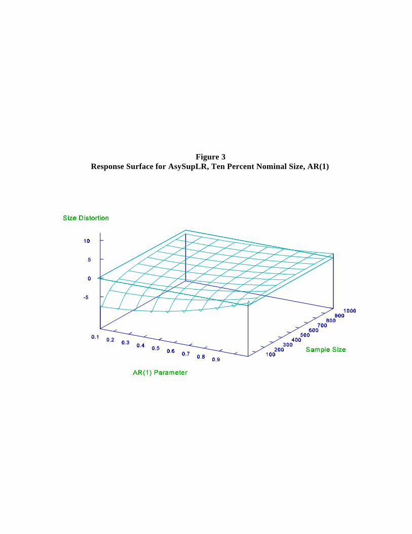
Figure 3Response Surface for AsySupLR, Ten Percent Nominal Size, AR(1)

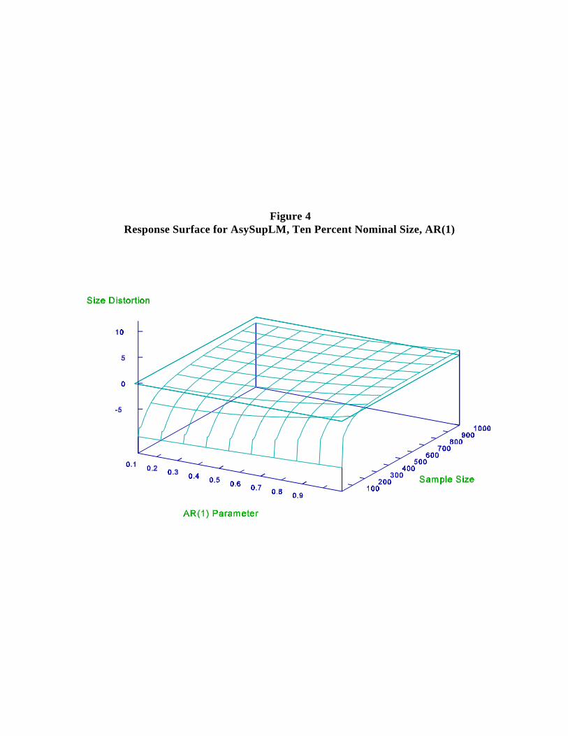
Figure 4Response Surface for AsySupLM, Ten Percent Nominal Size, AR(1)

Draw pseudo-innovationsConvert to pseudo-dataCompute test statistics

Draw true innovations Convert to true data Compute test statistics

Repeat RB times

Find critical value from bootstrap distribution

END

Repeat RM times

BootstrapLoop

Monte CarloLoop

Estimate empirical size as relative rejection frequency

Update rejection counter

Figure 5Flow Chart for Bootstrap Monte Carlo

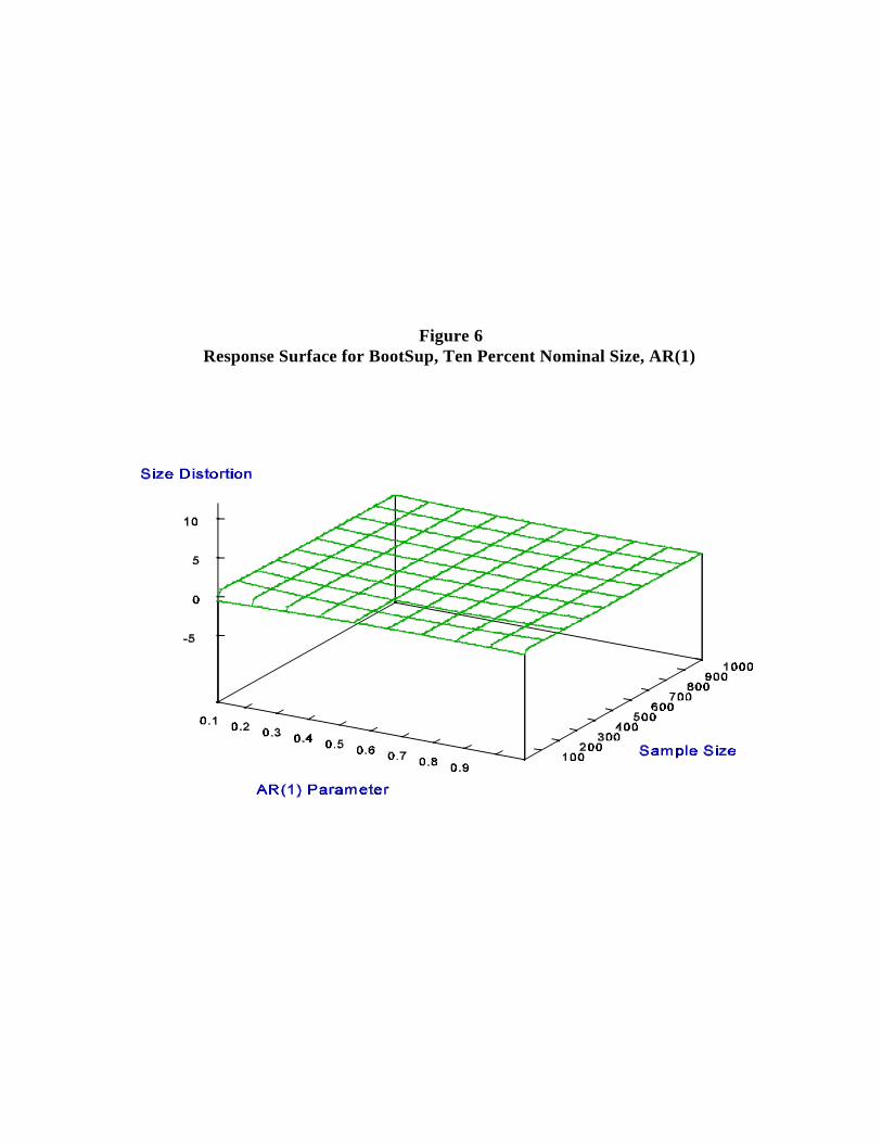
Figure 6Response Surface for BootSup, Ten Percent Nominal Size, AR(1)

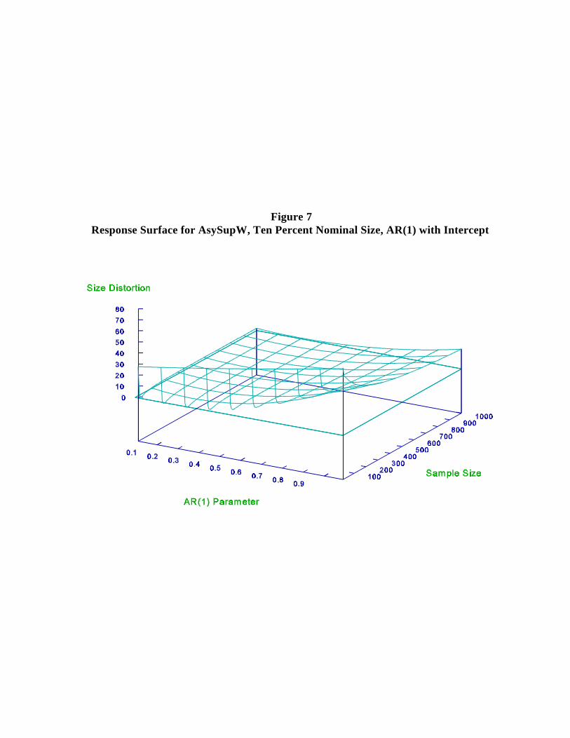
Figure 7Response Surface for AsySupW, Ten Percent Nominal Size, AR(1) with Intercept

Size Distortion

Figure 8Response Surface for BootSup, Ten Percent Nominal Size, AR(1) with Intercept

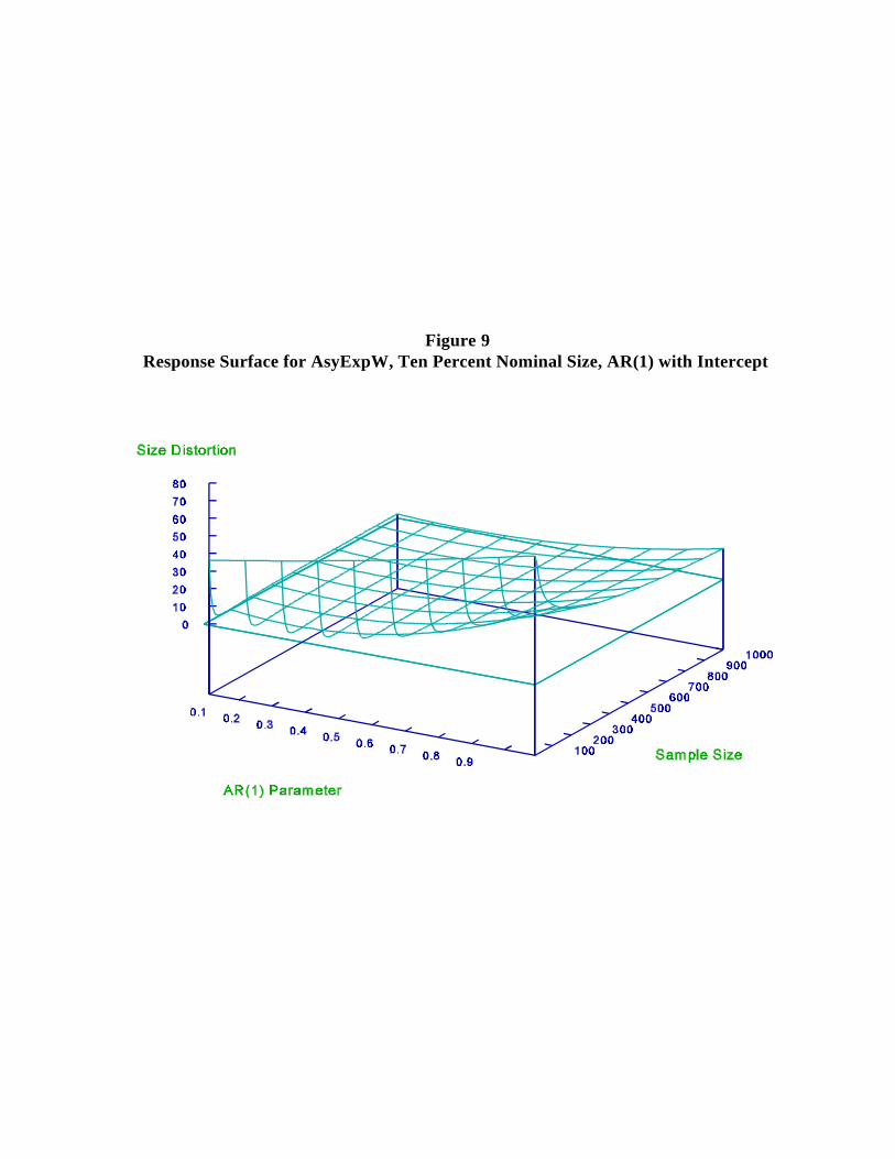
Figure 9Response Surface for AsyExpW, Ten Percent Nominal Size, AR(1) with Intercept

Size Distortion

Figure 10Response Surface for BootExpW, Ten Percent Nominal Size, AR(1) with Intercept

Notes to Tables and Figures

Table 1: The columns give the regressors for each response surface. T is sample size, is nominal test sizeand is the AR(1) parameter. All test names are of the form "xyz," where x denotes the type ofapproximation to the null distribution made ("Chi" for chi-squared, "Asy" for asymptotic and "Boot" forbootstrap), y denotes the type of test ("Sup" for supremum, "Exp" for exponential, and "Avg" for average),and z denotes the testing principle employed ("W" for Wald, "LR" for likelihood ratio, and "LM" forLagrange multiplier).

Table 2: T is sample size and is the AR(1) parameter. For each (T, ) pair, three nominal test sizes (1%,5%, 10%) are explored. See notes to Table 1 for test naming conventions.

Table 3: T is sample size and is the AR(1) parameter. For each (T, ) pair, three nominal test sizes (1%,5%, 10%) are explored. See notes to Table 1 for test naming conventions.

Table 4: The Wald, LR, LM results are identical, for reasons discussed in the text, so no distinction is madein the table. T is sample size and is the AR(1) parameter. For each (T, ) pair, three nominal test sizes(1%, 5%, 10%) are explored. See notes to Table 1 for test naming conventions.

All Figures: See notes to Table 1 for test naming conventions.