Testing of the CAPM Revisited - University of Washington · 1 Testing the CAPM Revisited 1. Introduction The Capital Asset Pricing Model (CAPM) of Sharpe (1964) and Lintner (1965)

Electronic copy available at: http://ssrn.com/abstract=1517874

TESTING THE CAPM REVISITED

Surajit Raya*

, N. E. Savinb and Ashish Tiwari

c

July 14, 2009

aMorgan Stanley, IM-Global Risk & Analysis, 522 5

th Avenue, New York, NY 10036*

bDepartment of Economics, Tippie College of Business, University of Iowa, 108 John Pappajohn

Bus. Bldg., Iowa City, IA 52242-1000 cDepartment of Finance, Tippie College of Business, University of Iowa, 108 John Pappajohn

Bus. Bldg., Iowa City, IA 52242-1000

Please send correspondence to: Ashish Tiwari, Tippie College of Business, Department of

Finance, 108 John Pappajohn Bus. Bldg., Iowa City, IA 52242-1000, USA. E-mail: ashish-

[email protected] Fax: (319) 335-3690. Tel: (319) 353-2185

* Morgan Stanley disclaimer: This information is for educational purposes only and does not contend to address the

financial objectives, situation or specific needs of any individual investor. Of course, these views may change in

response to changing circumstances and market conditions. This material has been prepared using sources of

information generally believed to be reliable. No representation can be made as to its accuracy. The forecasts and

opinions in this piece are not necessarily those of Morgan Stanley Investment Management, and may not actually

come to pass. Information in this report does not pertain to any Morgan Stanley Investment Management product

and is not a solicitation for any product.

Electronic copy available at: http://ssrn.com/abstract=1517874

Testing the CAPM Revisited

Abstract

This paper re-examines the tests of the Sharpe-Lintner Capital Asset Pricing Model (CAPM).

The null that the CAPM intercepts are zero is tested for ten size-based stock portfolios and for

twenty five book-to-market sorted portfolios using five-year, ten-year and longer sub-periods

during 1965-2004. The paper shows that the evidence for rejecting the CAPM on statistical

grounds is weaker than the consensus view suggests, and highlights the pitfalls of testing

multiple hypotheses with the conventional heteroskedasticity and autocorrelation robust (HAR)

test with asymptotic P-values. The conventional test rejects the null for almost all sub-periods,

which is consistent with the evidence in the literature. By contrast, the null is not rejected for

most of the sub-periods by the new HAR tests developed by Keifer, Vogelsang and Bunzel

(2000), Kiefer and Vogelsang (2005), and Sun, Phillips and Jin (2008).

1

Testing the CAPM Revisited

1. Introduction

The Capital Asset Pricing Model (CAPM) of Sharpe (1964) and Lintner (1965) rightfully

occupies a central place in the asset pricing literature. Not surprisingly, an enormous research

effort has been devoted to the empirical testing of the model over the past several decades.

Notwithstanding Roll’s (1977) famous critique of the early tests of the CAPM, a consensus now

exists that the model fails to adequately explain the cross-section of asset returns. The consensus

is supported by the results of several studies, most notably those by Fama and French (1992,

1996) and Campbell, Lo and MacKinlay (1997, hereafter CLM).

In this paper we re-examine the empirical evidence on the rejection of the CAPM by

CLM. The rejection of most interest is the one based on a conventional heteroskedasticity and

autocorrelation robust (HAR) test. Our main contribution is to show that the evidence for

rejecting the CAPM on statistical grounds is much weaker than the consensus view suggests.

Although it is well documented that the conventional HAR test rejects the CAPM using

asymptotic critical values, these results are not compelling because it is well known that the

conventional test suffers from size distortions when based on asymptotic P-values. In point of

fact, the evidence is much more favorable to the CAPM when inference is based on simulated

finite-sample P-values.

Next we revisit the CAPM using newly developed HAR tests (Sun, Phillips and Jin

(2008)). These tests have the advantage of substantially less size distortion relative to the

conventional robust tests. The results from these tests strongly support the CAPM when using

asymptotic as well as simulated finite-sample P-values. Our results highlight the pitfall of

2

testing multiple hypotheses with conventional HAR tests. This pitfall is one of potentially severe

over-rejection of the null hypothesis.

In HAR testing, the test statistics use kernel-based nonparametric estimators of the

standard deviations and covariances of the estimated regression coefficients. The test statistics

used in the conventional HAR tests incorporate heteroskedasticity and autocorrelation consistent

(HAC) estimators of the variance-covariance matrix. These estimators typically involve a

bandwidth or lag truncation parameter, M. Consistency requires that M satisfy certain conditions

as the sample size T increases. A commonly used HAC estimator is the one proposed by Newey

and West (1987, 1994). In applications, the finite sample distribution of a conventional HAR

test statistic is approximated by its asymptotic distribution, namely a standard normal or chi-

square. This approximation is known to be unsatisfactory in many cases, which gives rise to size

distortion, or more precisely, error in the rejection probability (ERP) under the null hypothesis.

To reduce the ERP, Keifer, Vogelsang and Bunzel (2000, hereafter KVB) and Keifer and

Vogelsang (2005, hereafter KV) proposed the use of kernel-based estimators in which M is set

proportional to the sample size T, that is, M bT . In this case, when the parameter b is fixed as

T goes to infinity, the kernel-based estimators have a random limiting distribution, which implies

that they are inconsistent. In turn, the associated test statistics have nonstandard limit

distributions. The nonstandard or new HAR tests are carried out in practice by approximating

the finite sample distribution of the test statistic by its nonstandard limit distribution.

In the Gaussian location model, Sun, Phillips and Jin (2008) have analyzed the ERP for

tests where b is fixed as T goes to infinity and where the critical values are obtained from the

nonstandard limit distribution. This ERP is compared to that for conventional tests with critical

values obtained from the standard normal approximation. They show that the ERP of the

3

nonstandard approximation is smaller than that of the standard normal approximation by an order

of magnitude. This result is an extension of an earlier finding by Jansson (2004). These

analytical findings support the earlier simulation results by KVB, KV (2002a, 20002b) and

Phillips, Sun and Jin (2006, 2007, hereafter PSJ). The conclusion from this analysis is that the

nonstandard approximation provides a substantially more accurate approximation to the finite

sample distribution. Consequently, the nonstandard test has substantially less size distortion than

the conventional test.

In this paper, we apply the conventional and new HAR tests to the CAPM using data for

the period 1965-2004. We applied the conventional and new HAR tests to settings with ten size-

sorted stock portfolios as well as settings with 15, 20 and 25 size and book-to-market sorted

portfolios. Consistent with the evidence in previous studies cited above, the conventional HAR

test with asymptotic P-values rejects the CAPM for most five-year and ten-year sub-periods at

the usual significance levels. By contrast, the null is not rejected by the new HAR tests with

asymptotic P-values for most of the sub-periods.

This finding is consistent with the results in Ray and Savin (2008). Their study used the

Fama-French three-factor model to illustrate that the new HAR tests can change inferences

drawn from the data and in particular that the conventional Wald tests tend to over-reject. In

contrast to the present study, Ray and Savin (2008) did not focus on the substantive issue of

whether the model is satisfactory for asset pricing.

One possible explanation for the conflicting results is that the conventional test has high

power compared to the new tests, assuming that the conventional test has the correct Type I error

or level in finite-samples. Another explanation for the conflict is that the conventional test over-

rejects instead of having the correct level. In other words, the actual finite-sample level of the

4

conventional test is much larger than the nominal level when asymptotic critical values are used,

or equivalently, the finite-sample P-value is substantially larger than the asymptotic P-value. We

conduct simulation experiments to investigate the source of the conflicting test results.

In the experiments for the conventional HAR test, the simulated finite-sample P-values

are larger than the asymptotic P-values, especially for the five-year and ten-year sub-periods,

which suggests that the conventional test over-rejects. The conflict between the conventional

test and the new tests for the five-year and ten-year sub-periods is much reduced when the tests

are based on simulated finite-sample P-values instead of asymptotic P-values. Moreover, the

new tests are clearly superior in terms of size distortion when many parameters are tested

simultaneously, which is the relevant case for testing the CAPM in a multi-portfolio framework.

In addition, the new tests have high power against empirically relevant alternatives.

These findings underscore the pitfalls of relying on inferences based on the conventional test.

Our results highlight that using the critical values or P-values based on the new tests can help to

mitigate the over-rejection problem.

The point that the conventional Wald tests and other related tests tend to over-reject the

null hypothesis is not new. Previous papers in the finance literature that have made this point

include Jobson and Korkie (1989), Gibbons, Ross and Shanken (1989), Zhou (1993), Kan and

Zhang (1999a, 1999b), Ahn and Gadarowski (2004) and Kan and Zhou (2002). However, these

papers do not provide satisfactory solutions to the poor finite-sample performance of the

conventional test.

Chief among these alternative approaches is the F-test of Gibbons, Ross and Shanken

(1989). It is well known that the finite-sample distribution for the GRS test statistic relies on the

assumption that returns are normally distributed and i.i.d., an assumption that is inconsistent with

5

the data. Another proposed solution is the test based on the Hansen and Jagannathan (1987)

distance measure. Kan and Zhou (2002) and Lewellen, Nagel, and Shanken (2008) derive the

exact finite sample distribution of the Hansen-Jagannathan distance measure. This finite sample

distribution again requires the assumption of multivariate normality of asset returns. As shown

by Kan and Zhou (2002) and Lewellen, Nagel, and Shanken (2008), in the absence of the

normality assumption, the test performs poorly. As noted by Cochrane (2005), “…it is not

obvious that a finite-sample distribution that ignores [non-normal and] non-i.i.d. returns will be a

better approximation than an asymptotic distribution that corrects for them (p. 302).” In

addition, the shortcomings of the conventional HAR test in asset pricing applications have been

noted by Ferson and Foerster (1994), and Hansen, Heaton, and Yaaron (1996). The new HAR

tests explored in this paper have the advantage that the nonstandard limiting distribution of the

test statistic provides a more accurate approximation to its finite sample distribution - a result

that has analytical justification.

Still another approach in the finance literature to overcome the shortcomings of the

conventional test has been pursued by Zhou (1993). He shows that the efficiency of the CRSP

value-weighted index is not rejected by a test that exploits the assumption that asset returns have

an elliptical distribution. A similar approach has been employed by Vorkink (2003). The test

employed by Vorkink accounts for the potential kurtosis in returns, although it does not account

for skewness. In contrast to these studies, this paper does not rely on alternative distributional

assumptions to achieve acceptance of the null hypothesis. In light of our findings, it is not

surprising that tests can be tailored such that the CAPM is not rejected.

The organization of the paper is the following. Section 2 reviews the conventional and

new HAR tests in the case of the location model. Section 3 presents the statistical framework

6

and the conventional and new HAR tests for testing the CAPM. Section 4 reports the CAPM test

results using the conventional HAR tests and the new HAR tests based on asymptotic P-values.

Section 5 gives the finite-sample P-values for the conventional and the new HAR tests and

Section 6 the simulated level-corrected powers. Section 7 reports the evidence on multivariate

complications and Section 8 concludes the paper.

2. HAR inference for the mean

The HAR tests are most easily introduced in the case of a simple location model. In the

context of this model, the HAR tests about the mean are conducted using t-statistics. An

advantage of the location model is that the properties of the conventional t-test and the

nonstandard or new t-tests can be analyzed analytically. Theoretical results on the accuracy of

the normal and the nonstandard approximations are reported, and the intuition behind the

superior performance of the new tests is discussed.

Following KVB and Jansson (2004), the focus of this section is on inference about in

the case of the location model:

, ( 1,..., )t ty u t T

where tu is a mean zero process with a nonparametric autocorrelation process. The least squares

estimator of gives 1

1

ˆ ,T

ttY T y

and the scaled and centered estimation error is

1/2 1/2ˆ( ) ,TT T S

where1

.t

tS u Let ˆu y be the time series of residuals. Under a commonly used

assumption about TS , the estimation error converges in distribution to a normal distribution:

2ˆ( ) (1) (0, ),T W N

7

which provides the usual basis for robust testing about . Here 2 is the long run variance of

and W(r) is standard Brownian motion.

The conventional approach is to estimate 2 using kernel-based nonparametric

estimators that involve some smoothing and possibly truncation of the autocovariances. When tu

is stationary with spectral density function ( ),uuf the long run variance (LRV) of tu is

2

0

1

2 ( ) 2 (0),uu

j

j f

where ( ) ( ).t t jj E u u The HAC estimates of 2 typically have the following form

11

12

11

1

ˆ ˆ for 0,ˆ ˆ ˆ( ) ( ) ( ), ( )

ˆ ˆ for 0,

T jT

t j tt

Tj T

t j tt j

T u u jjM k j j

M T u u j

involving the sample covariances ˆ( ).j In this expression, ( )k is some kernel; M is a bandwidth

parameter and consistency of 2ˆ ( )M requires M and / 0M T as ;T see, for

example, Andrews (1991), Hansen (1992) and Newey and West (1987, 1994).

To test the null 0 0:H against the alternative

1 0: ,H the conventional

approach relies on a nonparametrically studentized t-ratio statistic of the form

1/2

ˆ 0( )ˆ ˆ( ) / ( ),Mt T M

which is asymptotically (0,1)N . The use of this t-statistic is convenient empirically and is

widespread in practice, in spite of well-known problems with size distortion in inference.

To reduce size distortion, that is, the error in the rejection probability (ERP) under the

null, KVB and KV(2005) proposed the use of kernel-based estimators of 2 in which the

8

bandwidth parameter M is set equal to or proportional to T, that is, M bT for some 0,1b .

In this case, the estimator becomes

1

2

1

ˆ ˆ( ),T

b

j T

jk j

bT

and the associated t-statistic is given by

1/2

0ˆ ˆ( ) /b bt T .

The estimate ˆb is inconsistent and tends to a random quantity instead of , so the

bt -statistic is

no longer standard normal.

When the parameter b is fixed as T , KV showed that under suitable assumptions

2 2ˆb b , where the limit

b is random. Under the null hypothesis

1/2(1)b bt W .

Thus, the bt -statistic has a nonstandard limit distribution arising from the random limit of the

LRV estimate ˆb when b is fixed as T .

Sun, Phillips and Jin (2008) have obtained the properties of the tests analytically under

the assumption of normality. The assumption employed is that tu is a mean zero covariance

stationary Gaussian process with 2 | ( ) | .h

h h

The ERP of the nonstandard t-test with

fixed b is compared to that of the conventional t-test. The nonstandard test is based on the bt -

statistic and uses critical values obtained from the nonstandard limit distribution of 1/2(1) bW ,

while the conventional test is based on the ˆ ( )Mt -statistic and uses critical values from the

standard normal distribution. Sun et al. show that the ERP of the nonstandard test is 1( ),O T

while that of the conventional normal test is O(1). Hence, when b is fixed, the error of the

9

nonstandard approximation to the finite sample distribution of the bt -statistic under the null is

smaller than that of the standard normal approximation to the finite sample distribution of the

ˆ ( )Mt -statistic, again under the null. Moreover, the error of the nonstandard approximation is

smaller than that of the normal approximation by an order of magnitude.

This result is related to that of Jansson (2004), who showed that the ERP of the

nonstandard test based on the Bartlett kernel with b = 1 is O(logT/T). The Sun et al. (2008) result

generalizes Jansson’s result in two ways. First, it shows that the log (T) factor can be dropped.

Second, while Jansson’s result applies only to the Barlett kernel with b = 1, the Sun et al. result

applies to more general kernels than the Bartlett kernel and kernels with both b = 1 and b <1.

There are two reasons for the improved accuracy of the nonstandard approximation. One

is that the nonstandard distribution mimics the randomness of the denominator of the t-statistic.

In other words, the nonstandard test behaves in large samples more like its finite sample

analogue than the conventional asymptotic normal test. By contrast, the limit theory for the

conventional test treats the denominator of the t-ratio as if it were non-random in finite samples.

The other reason is that the nonstandard distribution accounts for the bias of the LRV estimator

resulting from the unobservability of the regressor errors, that is, the inconsistency mimics the

bias.

In related work, PSJ (2006,2007)) proposed an estimator of 2 of the form

1

2

1

ˆ ˆ( ) ( ),T

j T

jk j

T

which involves setting M equal to T and taking an arbitrary power 1 of the traditional kernel.

The associated t-statistic 1/2

0ˆ ˆ( ) /t T has a nonstandard limiting distribution arising

10

from the random limit of the estimator ˆ when is fixed as T . Statistical tests based on

2ˆb and 2ˆ

share many of the same properties, which is explained by the fact that and b play

similar roles in the construction of the estimates. An analysis of tests based on t is reported in

work by PSJ (2005a, 2005b).

3. HAR tests of the CAPM

This section considers the CAPM as a classical multivariate linear regression model with

random regressors and reviews the conventional and new HAR tests for the intercept vector.

Define the variables1,..., Ny y , where yi is the excess return for the ith portfolio or asset,

and the variable x where x is the market factor (the excess return on the market portfolio).

Suppose that the conditional expectation function is linear, ( | )E y x x ,

where 1 1 1( ,..., ) , ( ,..., ) and ( ,..., )N N Ny y y . The null hypothesis of interest

is0 : 0H , and the alternative is

1 : 0H . A nonzero value of the intercept is interpreted as

saying that the model leaves an unexplained return, a mean excess return that is unexplained by

the market factor.

Following Greene (2003), the multivariate regression model can be restated as a

seemingly unrelated regressions (SUR) model with identical regressors for the purpose of

presenting the classic and conventional robust Wald tests. Denote the tth observation on y

by1( ,..., )t t Nty y y

and on x by tx , (t =1,…,T). The SUR model is formulated using the N

regression equations , ( 1,..., ),i i iy X u i N where1( ,..., )i i iTy y y

, [ , ], (1,...,1) ,X x

1( ,..., ) , ( , ) ,T i i ix x x and

1( ,..., )i i iTu u u . Stacking the N regressions,

( ) ,y I X u Z u

11

where I is an NN identity matrix, 1( ,..., ) ,N and 1( ,..., )Nu u u . The least squares

estimator of is obtained by regressing y on Z. This produces the estimator

1ˆ ( ' ) 'Z Z Z y

1( ' ) 'Z Z Z u

.

Consider the scaled and centered estimator

1 1 1/2 1 1 1/2

1

ˆ( ) ( ' ) ( ' ) ( ( ' ))T

t

t

T T Z Z T Z u I T X X T v

,

where (1, )t t tv u x . Under general assumptions, for example, those given in KV and PSJ

(2005), the estimator converges in distribution to a normal:

1 1ˆ( ) (0, )T N Q Q

where 1( ( lim ' ))Q I p T X X and is the long run variance of t . In the case of the CAPM,

is a 2 2N N matrix

The conventional HAR statistic for testing the null hypothesis 0 : 0H is

1

1 1ˆ ˆˆˆ ˆ( )MW T RQ M Q R

,

where ˆ ( )M is an HAC estimator of and ˆ ˆˆ ( (1,0))I R . When 0 : 0H is true,

the test statistic is asymptotically distributed as a chi-square with N degrees of freedom; for

details, see KV.

The conventional approach to HAR testing relies on consistent estimation of the

sandwich variance matrix Q-1Q

-1. The term Q can be consistently estimated by

1ˆ ( ( ' )).Q I T X X When t is stationary with spectral density matrix ( )f , the LRV of

t

is

0

1

( ( ) ( ) ) 2 (0)vv

j

j j f

,

where ( ) ( )t t jj E . Consistent kernel-based estimators of are typically of the form

12

1

1

ˆ ˆ( ) ( ),T

j T

jM k j

M

1

1

1

1

ˆ ˆ for 0,ˆ ( )

ˆ ˆ for 0,

T j

t j tt

T

t j tt j

T jj

T j

which involves sample covariances ˆ ( )j based on estimates ˆ ˆ (1, )t t tv u x of

t that are

constructed from regression residuals ˆˆˆ ( )t t tu y x . The method proposed by ewey and

West (1987, 1994) is used to obtain the HAC estimator of for the conventional HAR test in

this paper.

The new Wald statistics used to test 0 : 0H are generalizations of the new t-statistics

for testing the mean, namely bt and t . When M bT , the kernel-based estimator of

becomes

1

1

ˆ ˆ ( ),T

b

j T

jk j

bT

and the associated test statistic is given by

1 1 1ˆ ˆˆˆ ˆ[ ]b bW T RQ Q R .

In the case of exponentiated or power kernels, the estimator of is

1

1

ˆ ˆ ( ),T

j T

jk j

T

and the associated test statistic is given by 1 1 1ˆ ˆˆˆ ˆ[ ]W T RQ Q R .

In this paper, two kernel functions are considered, both of which are commonly used in

practice. One is the Bartlett kernel,

(1 | |) | | 1,

( )0 | | 1,

x xk x

x

and the other is the Parzen kernel,

13

2 3

3

(1 6 6 | | ) for 0 | | 1/ 2,

( ) (2(1 | |) ) for 1/ 2 | | 1,

0 otherwise.

x x x

k x x x

Taking an arbitrary power 1 of these kernels gives the power kernels

(1 | |) | | 1,

( )0 | | 1,

x xk x

x

and

2 3

3

(1 6 6 | | ) for 0 | | 1/ 2,

( ) (2(1 | |) ) for 1/ 2 | | 1,

0 otherwise.

x x x

k x x x

The properties of the kernels are discussed in PSJ (2006, 2007).

4. Asymptotic test results

This section reports test results for the CAPM using the conventional HAR test and the

new HAR tests when the tests are based on asymptotic P-values. The asymptotic P-values are

obtained from the asymptotic chi-square distribution for the conventional test statisticMW and

the nonstandard asymptotic distributions for the new test statistics bW and W .

The return data consist of monthly returns, including distributions, for ten (N =10) CRSP

value-weighted portfolios of NYSE, AMEX and NASDAQ stocks. The stocks are assigned to

the portfolios based on market value of equity and annually rebalanced. The size-sorted portfolio

returns as well as the data for the market excess return and the one-month Treasury bill return are

taken from Ken French’s website. As will be noted below we also use the returns on the book-

to-market sorted stock portfolios available at the same website. The sample extends from

January 1965 through December 2004 (T = 480). The one-month Treasury bill is used as a

measure of the risk-free return. The tests are performed for five-year, ten-year, thirty-year sub-

14

periods and longer periods. The sub-periods include those used by CLM plus additional periods

made possible by more recent data.

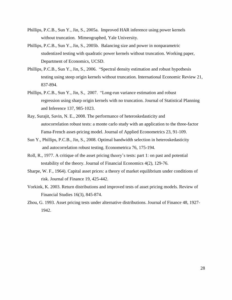
The asymptotic P-values for the conventional and new HAR tests are presented in Table

1. The asymptotic P-values for the conventional test reject the null at the 5 percent significance

level for all of the five-year and all but one of the ten-year sub-periods. Turning to the thirty-year

and longer sub-periods, the null is rejected for all six sub-periods. The Newey and West (1987,

1994) version of the conventional HAR test uses a HAC estimator based on the truncated Bartlett

kernel. The bandwidth for the tabled results is M = 6. The result are not qualitatively changed by

using M = 4. A well known guideline for choosing the bandwidth for the Bartlett kernel

is 1/30.75M T ; see Andrews (1991).

By contrast, the asymptotic P-values of the new HAR tests do not reject the null at the 5

percent significance level for more than one-half of the five-year sub-periods and for all of the

ten-year sub-periods with the exception of the 1995-2004 sub-period. The P-values for the fixed-

b tests are calculated using the Bartlett kernel and b =1 and those for the fixed- tests use the

Parzen kernel and = 32. The results are similar for values of b = 0.5 and for = 16. The null

is also not rejected by the asymptotic P-values for five out of six thirty-year and longer sub-

periods. It is worth emphasizing again that the limiting distributions of the fixed-b and fixed-

tests differ from chi-square distribution. In this application, relying on the fixed-b and fixed-

approximations produces fewer rejections than the conventional chi-square approximation.

5. Finite sample test results

As noted in the introduction, the main reason for thinking that results of the conventional

HAR test are problematic is that the asymptotic P-values of the new HAR tests do not reject the

null for the majority of the five-year, ten-year and longer sub-periods. The next step is to

15

investigate the finite-sample as opposed to the asymptotic performance of the conventional and

new HAR tests for each of the sub-periods. This section reports simulated finite-sample P-

values of the conventional and the new HAR tests where the P-values are calculated for the three

forms of the HAR test in four different experiments.

The null hypothesis that the intercepts are zero is composite because the values of the

nuisance parameters are unknown in practice. The nuisance parameters include not only the

slope parameters but also those that specify the process generating the factors and the errors. In

our experiments, the values of the nuisance parameters are set equal to estimates based on the

sample data. The level of the tests refers to the probability of a Type I error, not the size where

the latter is defined as the maximum level over all admissible values of the nuisance parameters.

In this paper, the simulated finite sample P-values are treated as exact, meaning that they are

conditional on the values of the nuisance parameters used in the designs. This should be borne in

mind when reviewing the discussion of the test results.

The experiments are now described for the January 1965 to 1969 sub-period. The value

ofty is simulated using the constrained least squares estimate of the conditional expectation

function (1) under the null:

* * * ( 1,..., ),t t ty x u t T

where*

ty ,*

tx , *

tu are the simulated values of ty ,

tx , tu and , the constrained least squares

estimates of the slope vectors calculated from the sample data for the sub-period.

Normal-Normal (NN) P-value experiment. This experiment produces data that satisfy

the assumptions of the classical normal SUR model with normally distributed regressors. The P-

value simulation procedure consists of five steps:

16

S1. Generate a sample of T = 60 *

tx vectors by randomly sampling the ( , )N x S

distribution where 1

ttx T x and 1 ( )( )t tt

S T x x x x are calculated

from sample data for the sub-period.


tu vectors independently of *

tx by randomly

sampling the (0, )N distribution where 1 ( )( )t ttT u u u u

and

1

ttu T u

are calculated from the constrained residual vectors

( )t t tu y x for the sub-period.


ty vectors from (9) using the*

tx vectors from

S1, the *

tu vectors from S2 and the constrained least squares estimates as the

values for the slope parameters.

S4. Compute the three forms of the HAR test statistic from the simulated dataset

of size T = 60.

S5. Repeat steps S1, S2, S3 and S4 10, 000 times. Compute the P-value for each

form of the HAR test statistic from the empirical distribution of the test statistic.

Resample-Resample (RR) P-value experiment. This experiment captures the

nonnormality present in the data. In this and the remaining experiments, only one or both of the

first two steps differ from those in the NN experiment.

S1 . Generate a sample of T = 60 *

tx vectors by randomly sampling with

replacement the observations tx .



tx by randomly

sampling with replacement the demeaned constrained least squares

residuals tu u .

Normal-VAR (NV) P-value experiment. This experiment introduces serial correlation

in the errors. The first step is the same as in the NN experiment.

17



tx using a

Gaussian VAR(1) process * * *

1t t tu u , where is a 10×10 matrix of

autoregressive coefficients. The autoregressive matrix is obtained by a least

squares regression of tuon

1tu using the constrained least square residuals for

the sub-period. The vector *

t is randomly sampled from the N(0, )

distribution, where 1

1( )( )

T

t ttT

and 1

ttT

are

calculated from the VAR residuals. The conditions for covariance-stationarity are

checked by calculating the roots of the matrix. In each replication, the initial

values of *

1tu in the VAR (1) are set equal to zero, and the first 200 draws are

discarded in order make the results independent of the initial values.

Resample-Block (RB) P-value experiment. This experiment allows for volatility

clustering of the returns. The first step is the same as in the RR experiment.



tx by randomly

sampling with replacement the demeaned constrained least squares

residuals tu u in consecutive fixed-length non-overlapping blocks where the

block length is six months.

The NN and RR experiments provide evidence on how the tests perform when the

multivariate iid assumption holds with and without normality. If the tests exhibit poor

performance under this assumption, it is unlikely that they will perform well in the presence of

autocorrelation or volatility clustering.

The rationale for the NV and RB experiments is the studies in finance documenting

departures from the iid assumption. The motivation for using a VAR(1) is the evidence reported

in CLM that individual securities have positive cross-autocorrelations. The RB experiments are

18

motivated by a large body of evidence that asset return volatility is both time-varying and

predictable; for example, see Bollerslev (1986) and Bollerslev, Engle and Nelson (1994).

In the simulation experiments, it was not feasible to generate the errors for each period

using an estimated multivariate GARCH model. Instead, we use a procedure that is employed in

bootstrap sampling with dependent data. The procedure is to divide the residual vectors for each

sub-period into blocks, and then randomly resample the blocks with replacement. In the RB

experiments, six-month length blocks were chosen because this is approximately the half-life of

an estimated univariate GARCH process for monthly stock returns; for example, see French,

Schwert and Stambaugh, (1987) for estimates for the period 1928-1984.

More generally, the RB experiments capture dependence in the errors. There are other

processes that may be generating dependence in addition to autoregressive conditional

heteroskedasticity. These include ARMA models and also models that produce non-martingale

difference sequences such as nonlinear moving average and bilinear models. Consequently, the

results of the RB experiments cannot be interpreted as only due to volatility clustering, although

this may be the dominant effect.

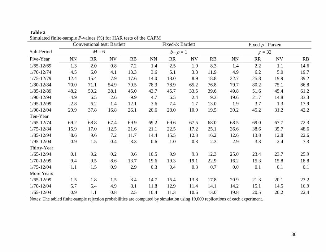
Table 2 presents the simulated finite-sample P-values for the conventional and new HAR

tests. The first message from this table is that the rejections of the null at the five percent level

are much reduced for the conventional test and are relatively few for the new HAR tests. For the

conventional test, the differences between the asymptotic and simulated finite-sample P-values

for the five-year sub-periods are quite large in all four experiments. This suggests that the

conventional test based on asymptotic P-values produces misleading inferences when testing the

CAPM. In point of fact, even for the thirty-year and longer sub-periods the conventional test

19

does not reject the null at the one percent level with few exceptions when inference is based on

the finite-sample P-values.

For the fixed-b and the fixed- tests, there is almost no conflict between the inferences

based on the asymptotic and simulated finite-sample P-values for the five-year and ten-year

periods. The same is true for the six thirty-year and longer sub-periods; the null is not rejected

for five out of six thirty-year and longer sub-periods based on asymptotic and finite-sample P-

values. Hence, the simulated finite-sample P-values and the asymptotic P-values produce

essentially the same inferences for the new HAR tests. In summary, the evidence in Table 2 is

largely supportive of the CAPM.

6. Power of new HAR tests

This section reports simulated level-corrected powers of the conventional and the new

HAR tests. The level-corrected powers are calculated for the three forms of the HAR test in four

different experiments. The four experiments are conducted for each of the sub-periods.

The simulated powers are estimates of the true level-corrected powers conditional on the

experimental design. The design specifies the vector of intercepts under the alternative, the

nuisance parameters including the slope vectors and the long run variance matrix and the process

generating the factors as well the errors.

The powers are calculated for a test of H0 against the alternative1 : (0.0005),H c

| | 0c . Here the alternative intercept vector is proportional to a vector of ones, , where c is a

scalar. With this setup, a unit increase in c translates into an increase in the monthly excess

return of 5 basis points. In finance a monthly excess return of 10 basis points (c = 2) is

20

considered small; see Fama and French (1996, p. 57). On the other hand, a monthly excess return

of 50 basis points (c = 10) is considered large by traditional benchmarks. One benchmark is the

equity premium. This is about 6 percent per annum, which translates into a monthly excess

return of 50 basis points. Another is the monthly excess return on the market portfolio, which is

between 80 and 100 basis points. Hence, this setup provides a natural metric for interpreting the

power, which is often absent in power studies.

The power experiments are now described for the January 1965 to 1969 sub-period. The

value ofty is simulated using

* * * ( 1,..., ),t t ty x u t T

where*

ty ,*

tx , *

tu are the simulated values of ty ,

tx , tu. The intercept vector is a known

constant given by the alternative H1. The slope is obtained by running a constrained least

squares regression of ont ty x for the sample data where the constraint is 0 .

Normal-Normal (NN) power experiment. The power simulation procedure consists of

four steps for each value of c. For c = 0, steps S1, S2, S3 and S4 are the same as in the P-value

simulation procedure. The fifth step is:

S5. Repeat steps S1, S2 S3, S4 10, 000 times. Compute the 5 percent critical value

for each form of the HAR test statistic from the empirical distribution of the test

statistic under H0 (c = 0).

For c ≥ 1, steps S1, S2, S3, S4 are the same as the P-value simulation procedure. The modified

fifth step is:

S5. Repeat steps S1, S2, S3 and S4 10,000 times. Compute the power for each

form of the HAR test statistic from the empirical distribution of the test statistic

using the simulated five percent critical value obtained from the c = 0 experiment.

The steps in the RR, NV and RB power simulation experiments are obtained by making

the analogous changes to the RR, NV and RB P-value simulation experiments.

21

The powers for the NN experiments for the conventional and new HAR tests are reported

in Table 3. The powers are reported only for positive values of c since the power curves are

symmetric in c. The results show that all three of the tests tend to have high level-corrected

power against empirically relevant departures from the null, that is, for monthly excess returns of

greater than 5 basis points. The level-corrected powers for T = 60 tend to be about 0.5 or greater

at c = 2 (monthly excess return of 10 basis points) and close to one at c = 3 (monthly excess

return of 15 basis points). The exceptions are the 1995-1999 and 2000-2004 sub-periods. The

powers of the three tests are very similar for 2c . The conventional test has generally higher

powers for the c = 1 case for the ten-year and longer periods. Nevertheless for empirically

relevant values of c, the Table 3 results show that the frequent non-rejections of the null by the

fixed-b tests and fixed- tests documented in Table 2 are not due to low power. The same

conclusion is supported by the results from the RR, NV and RB power experiments. These

results are available on request.

Table 3 shows that the powers do depend on the kernel and hence on choice of the HAR

test, although the results are qualitatively similar. Additional simulations show that the powers of

the fixed-b tests tend to increase as b decreases and the powers of the fixed-tests tend to

increase as increases. These results are consistent with the findings in KV(2005) and PSJ

(2006, 2007). However, this does not imply that a small b should be chosen for the fixed-b test or

a large for the fixed-test. This is because as b decreases the ERP of the fixed-b test increases

and as increases the ERP of the fixed-test increases. The trade-off between the ERP and

power is analyzed in detail in PSJ (2005a, 2005b) and Sun, Phillips and Jin (2008).

7. Multivariate complications

22

The purpose of this section is to convince readers who may have doubts about the

superiority of the new tests. This section reports the effect of increasing the number of intercepts

tested on the rejection probabilities of the conventional and new HAR tests. As will be seen, the

conventional HAR test suffers from massive size distortion when testing many intercepts

parameters simultaneously, which is relevant when testing the ten equation CAPM.

Ray and Savin (2008) considered a three-factor model with i equations and hence i

intercepts. In this section, we adapt their approach for the one-factor model. Accordingly, model

i is the CAPM with i equations:

( 1,...,10, 1,..., ),i i i i

t t ty x u i t T

where 1 1 1( ,..., ) , ( ,..., ), ( ,..., )i i i

t t it i iy y y and 1( ,..., )i

t t itu u u . The ordering of

the models and equations makes use of the fact that the portfolios are ordered by market equity.

The ith intercept is the intercept of the equation for the ith portfolio of stocks.

For the ith model, the null hypothesis of interest is 0 : 0i iH , and the alternative

is 1 : 0i iH . The null 0

iH is tested for the ith model using the conventional, fixed-b and fixed-

tests with five percent asymptotic critical values. The finite-sample levels of the tests for the ith

model are obtained by simulation. In the simulation experiments, the null 0 : 0i iH is imposed.

In the ith model, the value ofty is simulated using

* * * ( 1,...,10, 1,..., ),i i i

t t ty x u i t T

where * * *, , i i

t t ty x u are the simulated values of , , i i

t t ty x u and ,i is the constrained least

squares estimate of the slope vector. The slope estimates are calculated using the data for January

1965 through December 2004. The rejection probabilities are simulated for T = 60, 120 and 240.

23

Ray and Savin give the detailed simulation procedure for the NN probability experiments in the

case of the three-factor model. The modifications for the one-factor model are straightforward.

Panel A of Table 4 reports the results for the NN experiments when the tests use five

percent asymptotic critical values. The results for the Bartlett-based conventional robust test

with M = 6 show that the number of intercept parameters has a very strong effect on the

simulated levels. The results for T = 60 show that the ERP is about 5 percent for the one

equation model and 66 percent for the ten equation model, about a thirteen-fold increase in the

ERP as the number of intercept parameters tested is increased from one to ten. Given T = 120,

the ERP is about 2 percent for the one equation model and about 32 percent for all ten equations.

In this case, although the ERP is not large for one parameter, it is very substantial for ten

parameters.

Next compare the effect of the number of intercepts on the level of the fixed-b and fixed-

test. For the fixed-b test, the effect of the number of intercepts is almost eliminated, and

similarly for the fixed- test with = 32. For T = 60, the ERP is about 1 percent or less for the

one equation model and about 2 percent for the ten equation model. For T = 120, the ERP tends

to be less than 1 percent for all ten equations.

Panel B of Table 4 reports the results for alternative experimental designs in addition to

the NN design for the ten equations case. For the alternative experiments, the ERPs are larger

than for the NN experiments. The difference is especially noticeable for the NV and RB

experiments, that is, experiments that allow for serial correlation and/or volatility clustering.

Nevertheless, even for these experiments, the new tests exhibit substantially lower ERPs

compared to the conventional test. Note that even for T = 480 the conventional test has an ERP

ranging from 5 percent for the NN experiment to twenty five percent for the NV experiment.

24

This further illustrates that the rejections of the CAPM documented in the literature need to be

viewed with caution.

As a robustness check, we also applied the conventional and new HAR tests to settings

with more than ten portfolios, namely the 15, 20 and 25 size and book-to-market sorted

portfolios obtained from the Ken French website. For the NN experiments, the results show that

the P-values for the conventional tests are zero for all three sets of portfolios for all sub-periods.

In contrast, the P-values are frequently above 5 per cent for the majority of the fixed- tests and

about for about half of the fixed-b tests. This evidence again suggests that the conventional test

leads to an over-rejection of the null hypothesis. By contrast, the new tests are clearly superior in

terms of size distortion when many parameters are tested simultaneously.

8. Concluding comments

In this paper, we have assumed that the conditional expectation function (CEF) of a stock

portfolio’s return given the market return (i.e., the CEF of giveny x ) is linear. Although this

assumption is not in general compatible with the three-factor Fama-French (1993) model and the

four-factor Carhart (1997) model, the CAPM can be interpreted as the population linear

projection of ony x or best linear predictor of giveny x . In this interpretation, the Sharpe-

Lintner version of the CAPM implies that all the elements in the intercept of the best linear

predictor are zero, and the HAR tests can be interpreted as testing the intercept of the best linear

predictor.

With this interpretation in mind, our study finds that the evidence for the statistical

rejection of the CAPM is weaker than the consensus view suggests. This finding illustrates the

pitfalls of testing multiple hypotheses with the conventional HAR test. The potential solution to

the over-rejection problem is to use the new HAR tests employed in this paper.

25

Acknowledgements

We are grateful to the editor and to two anonymous referees for constructive comments

and suggestions. The result has been a substantially improved version of the paper.

26

References

Ahn, S. C., Gadarowski C., 2004. Small sample properties of the GMM specification test

based on the Hansen-Jagannathan distance. Journal of Empirical Finance 11, 109-132.

Andrews, D.W. K., 1991. Heteroskedasticity and autocorrelation consistent covariance matrix

estimation. Econometrica 59, 817-854.

Bollerslev, T., 1986. Generalized autoregressive conditional heteroskedasticity. Journal of

Econometrics 31, 307-327.

Bollerslev, T., Engle, R. R., Nelson, D.B., 1994. Arch models. In Engle, R. R., McFadden, D.L.

(Ed.), Handbook of Econometrics, vol. 4, North-Holland, Amsterdam, 2961-2984.

Campbell, J.Y., Lo, A. W., MacKinlay, A.C., 1997. The econometrics of financial markets.

Princeton University Press, Princeton, New Jersey.

Carhart, M., 1997. On persistence in mutual fund performance. Journal of Finance 52, 57-82.

Cochrane, J.H., 2005. Asset pricing. Princeton University Press, Princeton, New Jersey.

Fama, E.F., French, K.R., 1992. The cross-section of expected stock returns. Journal of Finance

47, 427-465.

Fama, E.F., French, K.R., 1993. Common risk factors in the returns on stocks and bonds.

Journal of Financial Economics 33, 3-56.

Fama, E.F., French, K.R., 1996. Multifactor explanations of asset pricing anomalies. The

Journal of Finance 51, 55-83.

Ferson, W.E., Foerster, S.R., 1994. Finite sample properties of the generalized method of

moments in tests of conditional asset pricing models. Journal of Financial Economics 36,

29– 55.

French, K.R., Schwert, G. W., Stambaugh., R.F., 1987. Expected stock returns and volatility.

Journal of Financial Economics 19, 3-30.

Gibbons, M., Ross, S., Shanken. J., 1989. A test of the efficiency of a given portfolio.

Econometrica 57, 1121-1152.

Greene, W. H., 2003. Econometric Analysis, fifth edition. Prentice Hall New Jersey.

Hansen, B.E., 1992. Consistent covariance matrix estimation for dependent heterogeneous

Process. Econometrica, 60, 967-972.

Hansen, L.P., Jagannathan, R., 1997. Assessing specification errors in stochastic discount

27

factor models. Journal of Finance 52, 557-590.

Hansen, L.P., Heaton, J., Yaaron, A., 1996. Finite-sample properties of some alternative

GMM estimators. Journal of Business and Economic Statistics 14(3), 262-80.

Jansson, M., 2004. “The error in rejection probability of simple autocorrelation robust tests.


Jobson, J. D., Korkie, B., 1989. A performance interpretation of multivariate tests of asset

set intersection, spanning, and mean variance efficiency. Journal of Financial and

Quantitative Analysis 24, 185-204.

Kan, R., Zhang, C., 1999. GMM tests of stochastic discount factor models with useless

factors. Journal of Financial Economics 54, 103–127.

Kan, R., Zhang, C., 1999. Two-pass tests of asset pricing models with useless factors.

Journal of Finance 54, 204–235.

Kan, R., Zhou, G., 2002. Hansen-Jagannathan distance: geometry and exact distribution,

Working paper, University of Toronto and Washington University, St. Louis.

Kiefer, N. M., Vogelsang, T.J., 2002a. Heteroskedasticity –autocorrelation robust testing using

bandwidth equal to sample size. Econometric Theory 18, 1350-1366.

Kiefer, N. M., Vogelsang, T.J., 2002b. Heteroskedasticity –autocorrelation robust standard

errors using the Bartlett Kernel without truncation. Econometrica 70, 2093-2095.

Kiefer, N. M., Vogelsang, T.J., 2005. A new asymptotic theory for heteroskedasticity-

autocorrelation robust tests. Econometric Theory 21, 1130-1164.

Kiefer, N. M., Vogelsang, T.J., Bunzel, H., 2000. Simple robust testing of regression hypotheses.


Lewellen, J; Nagel, S., Shanken, J., 2008. A skeptical appraisal of asset-pricing tests.

Working paper, Dartmouth College.

Lintner, J., 1965. The valuation of risk assets and the selection of risky investments in stock

portfolios and capital budgets. Review of Economics and Statistics 47, 13-37.

Newey, W.K, West, K.D., 1987. A simple, positive semi-definite, heteroskedasticity and

autocorrelation consistent covariance matrix. Econometrica 55, 703-708.

Newey, W.K, West, K.D., 1994. Automatic lag selection in covariance estimation. Review of

Economics Studies 61, 631-654.

28

Phillips, P.C.B., Sun Y., Jin, S., 2005a. Improved HAR inference using power kernels

without truncation. Mimeographed, Yale University.

Phillips, P.C.B., Sun Y., Jin, S., 2005b. Balancing size and power in nonparametric

studentized testing with quadratic power kernels without truncation. Working paper,

Department of Economics, UCSD.

Phillips, P.C.B., Sun Y., Jin, S., 2006. “Spectral density estimation and robust hypothesis

testing using steep origin kernels without truncation. International Economic Review 21,

837-894.

Phillips, P.C.B., Sun Y., Jin, S., 2007. “Long-run variance estimation and robust

regression using sharp origin kernels with no truncation. Journal of Statistical Planning

and Inference 137, 985-1023.

Ray, Surajit, Savin, N. E., 2008. The performance of heteroskedasticity and

autocorrelation robust tests: a monte carlo study with an application to the three-factor

Fama-French asset-pricing model. Journal of Applied Econometrics 23, 91-109.

Sun Y., Phillips, P.C.B., Jin, S., 2008. Optimal bandwidth selection in heteroskedasticity

and autocorrelation robust testing. Econometrica 76, 175-194.

Roll, R., 1977. A critique of the asset pricing theory’s tests: part 1: on past and potential

testability of the theory. Journal of Financial Economics 4(2), 129-76.

Sharpe, W. F., 1964). Capital asset prices: a theory of market equilibrium under conditions of

risk. Journal of Finance 19, 425-442.

Vorkink, K. 2003. Return distributions and improved tests of asset pricing models. Review of

Financial Studies 16(3), 845-874.

Zhou, G. 1993. Asset pricing tests under alternative distributions. Journal of Finance 48, 1927-

1942.

29

Table 1

Asymptotic P-values (%) for HAR tests of the CAPM

Notes: The tabled asymptotic P-values for the fixed-b and fixed- tests are computed by simulation using

10,000 replications of each experiment. The P-values for the conventional HAR test are calculated from

the chi-square distribution with ten degrees of freedom.

Conventional: Barlett Fixed-b: Barlett Fixed-: Parzen

Sub-Period WM

M = 6

P-value Wb

b = 1

P-value W

= 32

P-value

Five-Year

1/65-12/69 98.23 0.0000 725.96 0.0094 205.88 0.0153

1/70-12/74 73.68 0.0000 619.46 0.0230 141.22 0.0442

1/75-12/79 54.81 0.0000 416.86 0.1003 72.46 0.2087

1/80-12/84 18.73 0.0438 125.17 0.7473 21.46 0.7859

1/85-12/89 27.75 0.0020 240.66 0.3619 41.47 0.4692

1/90-12/94 71.94 0.0000 579.11 0.0304 77.98 0.1811

1/95-12/99 90.26 0.0000 684.98 0.0129 214.26 0.0141

1/00-12/04 36.23 0.0001 348.34 0.1607 49.67 0.3771

Ten-Year

1/65-12/74 11.50 0.3196 144.88 0.6696 27.16 0.6866

1/75-12/84 26.16 0.0035 330.44 0.1855 50.69 0.3681

1/85-12/94 31.31 0.0005 381.86 0.1294 92.63 0.1279

1/95-12/04 50.79 0.0000 815.90 0.0051 170.30 0.0254

Thirty-Year

1/65-12/94 37.05 0.0001 420.69 0.0971 66.52 0.2417

1/70-12/99 19.89 0.0303 332.55 0.1827 83.16 0.1595

1/75-12/04 29.14 0.0012 911.13 0.0027 507.80 0.0004

More Years

1/65-12/99 26.75 0.0029 370.06 0.1399 71.94 0.2123

1/70-12/04 21.66 0.0169 399.33 0.1152 86.90 0.1459

1/65-12/04 27.84 0.0019 415.68 0.1012 74.42 0.1989

30

Table 2

Simulated finite-sample P-values (%) for HAR tests of the CAPM

Notes: The tabled finite-sample rejection probabilities are computed by simulation using 10,000 replications of each experiment.

Conventional test: Bartlett Fixed-b: Bartlett Fixed- : Parzen

Sub-Period M = 6 b= 1 = 32

Five-Year NN RR NV RB NN RR NV RB NN RR NV RB

1/65-12/69 1.3 2.0 0.8 7.2 1.4 2.5 1.0 8.3 1.4 2.2 1.1 14.6

1/70-12/74 4.5 6.0 4.1 13.3 3.6 5.1 3.3 11.9 4.9 6.2 5.0 19.7

1/75-12/79 12.4 15.4 7.9 17.6 14.0 18.0 8.9 18.8 22.7 25.8 19.9 39.2

1/80-12/84 70.0 71.1 54.9 70.5 78.3 78.9 65.2 76.8 79.7 80.2 75.1 86.8

1/85-12/89 48.2 50.2 38.1 45.0 43.7 45.7 33.5 39.6 49.8 51.6 45.4 61.2

1/90-12/94 4.9 6.5 2.6 9.9 4.7 6.5 2.4 9.3 19.6 21.7 14.8 33.3

1/95-12/99 2.8 6.2 1.4 12.1 3.6 7.4 1.7 13.0 1.9 3.7 1.3 17.9

1/00-12/04 29.9 37.8 16.8 26.1 20.6 28.0 10.9 19.5 39.2 45.2 31.2 42.2

Ten-Year

1/65-12/74 69.2 68.8 67.4 69.9 69.2 69.6 67.5 68.0 68.5 69.0 67.7 72.3

1/75-12/84 15.9 17.0 12.5 21.6 21.1 22.5 17.2 25.1 36.6 38.6 35.7 48.6

1/85-12/94 8.6 9.6 7.2 11.7 14.4 15.5 12.3 16.2 12.6 13.8 12.8 22.6

1/95-12/04 0.9 1.5 0.4 3.3 0.6 1.0 0.3 2.3 2.9 3.3 2.4 7.3

Thirty-Year

1/65-12/94 0.1 0.2 0.2 0.6 10.5 9.9 9.3 12.3 25.0 23.4 23.7 25.9

1/70-12/99 9.4 9.5 8.6 13.7 19.6 19.3 19.1 22.9 16.2 15.3 15.8 18.8

1/75-12/04 1.1 1.5 0.9 2.9 0.3 0.4 0.3 0.7 0.0 0.1 0.1 0.1

More Years

1/65-12/99 1.5 1.8 1.5 3.4 14.7 15.4 13.8 17.8 20.9 21.3 20.1 23.2

1/70-12/04 5.7 6.4 4.9 8.1 11.8 12.9 11.4 14.1 14.2 15.1 14.5 16.9

1/65-12/04 0.9 1.1 0.8 2.5 10.4 11.3 10.6 13.0 19.8 20.5 20.2 22.4

31

Table 3

Simulated power (%) of level-corrected 5 percent new HAR tests for the NN experiments

Notes: The tabled finite-sample powers are computed by simulation using 10,000 replications of each experiment. In each power

experiment the simulated monthly stock portfolio returns under the alternative are characterized by a non-zero CAPM intercept or

model pricing error. The powers calculations are based on intercept values that are equal to c times 5 basis points per month.

Conventional test: Bartlett Fixed-b: Bartlett Fixed- : Parzen

Sub-Period M = 6 b= 1 = 32, b =1

Five-Year c = 1 c = 2 c = 3 c = 4 c = 1 c = 2 c = 3 c = 4 c = 1 c = 2 c = 3 c = 4

1/65-12/69 38.2 93.8 99.9 100.0 38.8 93.1 99.8 100.0 27.7 80.3 98.4 100.0

1/70-12/74 42.3 96.4 100.0 100.0 43.5 95.4 99.8 100.0 31.6 85.9 99.2 100.0

1/75-12/79 22.2 76.5 98.3 100.0 22.4 76.4 97.5 99.8 16.8 58.0 90.4 98.9

1/80-12/84 22.0 74.6 98.1 99.9 22.1 73.7 97.0 99.8 16.7 56.3 89.0 98.7

1/85-12/89 49.7 98.5 100.0 100.0 50.6 97.7 99.9 100.0 36.0 90.7 99.8 100.0

1/90-12/94 40.8 96.3 100.0 100.0 41.1 95.1 99.9 100.0 29.4 84.8 99.2 100.0

1/95-12/99 12.6 44.7 81.7 96.7 13.0 45.5 82.0 96.1 10.4 32.4 65.0 87.3

1/00-12/04 7.4 17.5 38.7 64.6 7.4 18.1 39.8 65.7 6.8 13.9 27.5 47.1

Ten-Year

1/65-12/74 73.2 100.0 100.0 100.0 62.8 99.4 100.0 100.0 44.5 95.7 100.0 100.0

1/75-12/84 28.5 89.4 99.9 100.0 25.6 80.0 98.2 99.9 17.9 59.9 91.2 99.2

1/85-12/94 72.5 100.0 100.0 100.0 61.1 99.2 100.0 100.0 43.1 95.7 99.9 100.0

1/95-12/04 14.1 55.9 93.1 99.8 13.4 47.9 84.3 96.9 10.7 32.0 64.0 87.8

Thirty-Year

1/65-12/94 94.4 100.0 100.0 100.0 77.4 99.9 100.0 100.0 57.2 98.7 100.0 100.0

1/70-12/99 91.4 100.0 100.0 100.0 71.8 99.6 100.0 100.0 51.0 97.8 100.0 100.0

1/75-12/04 71.8 100.0 100.0 100.0 52.4 98.1 100.0 100.0 35.3 90.3 99.7 100.0

More Years

1/65-12/99 96.8 100.0 100.0 100.0 81.2 99.9 100.0 100.0 60.2 99.2 100.0 100.0

1/70-12/04 83.7 100.0 100.0 100.0 63.1 99.3 100.0 100.0 44.9 95.7 99.9 100.0

1/65-12/04 92.8 100.0 100.0 100.0 72.3 99.7 100.0 100.0 52.9 98.2 100.0 100.0

32

Table 4

Simulated rejection probabilities (%) of nominal 5 percent HAR tests by equation subsets

Panel A: NN experiments

Conventional

Bartlett

M = 6

Fixed-b: Bartlett

b= 1

Fixed- Parzen

= 32

Equations

T = 60

1 9.6 5.6 4.8

1-2 13.6 5.2 5.2

1-3 18.5 5.6 5.1

1-4 23.8 5.5 5.2

1-5 30.7 5.4 5.3

1-6 38.7 5.8 5.5

1-7 47.0 6.4 5.7

1-8 54.7 6.0 5.8

1-9 63.5 7.4 6.1

1-10 71.2 7.2 5.7

T =120

1 6.7 5.3 4.8

1-2 8.9 5.0 5.2

1-3 11.0 5.5 5.0

1-4 13.2 5.2 4.9

1-5 15.5 4.8 4.8

1-6 18.8 5.1 5.1

1-7 23.3 5.1 5.0

1-8 28.0 6.4 6.4

1-9 31.8 5.6 5.2

1-10 36.5 5.3 5.0

33

Panel B: Alternative experiments for the 10 equations case

Conventional

Bartlett

M = 6

Fixed-b: Bartlett

b= 1

Fixed- Parzen

= 32

Experiment

T = 60

NN 71.2 7.2 5.7

RR 72.4 7.6 5.9

NV 85.9 30.0 21.7

RB 79.4 16.9 12.7

T = 120

NN 36.5 5.3 5.0

RR 38.5 6.0 5.5

NV 59.6 17.7 12.3

RB 47.6 10.9 8.8

T = 360

NN 13.8 4.7 4.9

RR 13.5 4.8 4.9

NV 34.6 9.1 7.0

RB 19.1 7.3 6.2

T = 480

NN 10.1 5.0 4.9

RR 10.7 5.0 4.9

NV 30.3 8.1 6.0

RB 15.7 7.2 6.1

Notes: The tabled rejection probabilities are computed by simulation using 10,000

replications of each experiment.

Documents

Testing of the CAPM Revisited - University of Washington · 1 Testing the CAPM Revisited 1. Introduction The Capital Asset Pricing Model (CAPM) of Sharpe (1964) and Lintner (1965)