Embed Size (px)
Citation preview

1
In Germany the CAPM is Alive and Well†
Roman Brückner* / Patrick Lehmann
* /Richard Stehle
*
February 2012
Draft: Please do not cite without our permission.
The “official” first draft will be available on SSRN by April 2012.
Abstract
Using data on all firms listed in the top segment of the Frankfurt Stock Exchange during the
years 1960 to 2007, we investigate how the (Sharpe-Lintner) CAPM performs under the as-
sumption that the German capital market is totally segmented from other capital markets. We
also check whether this model should be extended by the firm characteristics size and book-
to-market. We can identify strong size and book-to-market effects in the German stock mar-
ket. However, their direction, strength, and interaction are different in the two sub-periods
1960 - 1990 and 1990 - 2007.
We use the standard test procedures (BJS, GRS, Fama/MacBeth) to test the CAPM and do a
large number of tests which differ by the length of the test period, the length of the return
interval, beta calculations, firm level and portfolio data, sorting, and weighting. The total
number of CAPM rejections is somewhat higher than what we would expect based on the
statistical significance level. Long-term GRS tests often lead to rejections of the CAPM, es-
pecially in the second sub-period and in sorts on anomalies. Short term GRS-tests always
reject the CAPM during the years 2000 to 2005. The results of Fama/MacBeth cross-
sectional regressions depend on sorting, weighting and beta calculation. When we sort on
beta and use value-weight portfolios the results for the full period 1960 to 2007 are fully in
line with the CAPM.
Our interpretation of the results is that in Germany the pure domestic version of the CAPM
works better than an extended model. It works better for large firms than for small firms.
Possibly the input data suits large firms better.
† Similar titles have been used by Jagannathan/Wang (1996) for an earlier working paper and by Levy (2010).
* Humboldt University Berlin, School of Business and Economics, Institute for Banking, Stock Exchanges and
Insurances, Dorotheenstr. 1, D - 10099 Berlin. Phone.: +49 [30] 2093-5661, Fax: +49 [30] 2093-5666.
E-Mail: [email protected], [email protected], [email protected].

2
1. Introduction and Conclusion
The capital asset pricing model (CAPM) of Sharpe (1964) and Lintner (1965) has been dis-
cussed, tested and applied during the last 50 years, first in the U.S, then around the world.1
To our knowledge, it has been used extensively for calculating the equity cost of capital in
Germany during the past 10 years.2 In these applications, it is typically assumed that the
German stock market is totally segmented from other markets. That is, the German risk free
rate, an estimate for the German risk premium, and “German” betas are used. A recent appli-
cation assumed an integrated European capital market. Especially well-documented is the
models use in legal proceedings on the freeze-out of minority shareholders,3 in network regu-
lation,4 and in the evaluation of mutual fund performance.
5 Following the ”worldwide” dis-
cussion of CAPM anomalies, it is discussed in Germany in all three areas whether the CAPM
should be extended by the two most prominent anomaly variables, size and book-to-market
(ratio) or by factors that represent these characteristics.6 In the area of mutual fund evalua-
tion, momentum is considered as an additional explanatory variable. It is also being dis-
cussed, whether the Sharpe-Lintner model should be interpreted nationally or internationally7
and/or whether it should be replaced by another asset pricing model, e.g. the after-tax
1 We follow the literature and use the acronym CAPM only to refer to the model originally proposed by
Sharpe (1964) and Lintner (1965), see Fama/French (2004), FN 1. We use the CAPM and the Sharpe-
Lintner model as synonyms. 2 A prominent supporter of the CAPM has been the German monopoly watchdog, the Monopolkommission.
3 In Germany, the term ´squeeze-out` is typically used. Squeeze-outs of minority shareholders were regulated
by the `Wertpapiererwerbs- und Übernahmegesetz´ in 2002. The OLG (Regional Appeal Court) Düsseldorf
decided e.g. on May 27th
, 2009 (I-26W 5/07) that presently the Sharpe-Lintner CAPM is the most important
model for the estimation of the cost of capital for valuation purposes. The OLG Stuttgart discussed the ap-
propriate risk premium extensively in its decision dated May 4th
, 2011 (20 W 11/08). Typically, the court
decisions are based on company valuation appraisals prepared by public accountants, who typically are
members of the Institut der Wirtschaftsprüfer in Deutschland e.V. (IDW). The IDW recommends the CAPM
since XXXX. Typically German public accountants follow the recommendation of the IDW. 4 Presently the CAPM is used in the network regulation areas telecommunication, gas, and electric power. The
mobile phone termination fee, e.g. is based on the CAPM since December 1st, 2010 (Beschluss BK 3a-
10/100, dated February 24th
, 2011), the fixed line termination fee since April 1st, 2011 (Beschluss BK 3c-
11/003, dated March 3rd
, 2011). Here, a European beta and an international risk premium are used.
Sudarsanam (2011) reviews the models use in many other countries. 5 Among academics as well as practitioners, Jensen’s alpha is probably one of the best-known and still widely
used performance measures for evaluating the success of mutual fund managers. It is calculated as the dif-
ference between the average portfolio return and its risk adjusted model return of the CAPM. In the academ-
ic literature Jensen’s alpha is still used in performance evaluation studies––at least in addition to more com-
prehensive models like the Fama/French three-factor model or the Carhart four-factor model (see for exam-
ple the recent articles by Evans (2010) and Fama/French (2010)). It is also displayed in publicly available
fund information systems (e.g. Morningstar). 6 Other anomalies such as momentum have received great attention in the literature. Recent articles about the
momentum effect include Bulkley/Nawosah (2009) and Fama/French (2008). 7 The CAPM may be interpreted nationally or internationally, see Stehle (1977). In this paper we concentrate
on the pure national interpretation. Fama/French (2011) argue that local models work better than global
models, especially if the model includes factors.
3
CAPM,8 a more complicated international CAPM,
9 the zero-beta CAPM, or a combination of
these models.
We use data for the top segment of the Frankfurt Stock Exchange for the period from 1960 to
2007 to investigate how the Sharpe-Lintner CAPM performs under the assumption that the
German capital market is totally segmented from other capital markets. We also check
whether this model should be extended by the firm characteristics size and book-to-market.
We focus on the two most important anomaly variables because we believe that the estima-
tion of the equity cost of capital is the most important application of the model.10
We use the time-series test proposed by Jensen (1968) and Black/Jensen/Scholes (1972), and
the cross-sectional test proposed by Fama/MacBeth (1973). These were refined in a large
number of studies, notably by Fama/French (1992) and Gibbons/Ross/Shanken (1989). Since
the three procedures are based on different assumptions and test objectives, and look at the
time-series of cross-sectional data in different ways, we consider them as ideal complements
to each other, especially when the same set of test portfolios are used, which we plan to do.
There already exist several studies that apply variations of these procedures to German data,
most recently Artmann/Finter/Kempf/Koch/Theissen (2012), Amel-Zadeh (2011), Artmann/-
Finter/Kempf (2010), and Schrimpf/Schröder/Stehle (2007). These studies typically find that
extended models describe the cross-section of returns “better” than the Sharpe-Lintner model.
Artmann/Finter/Kempf (2010) even conclude that the CAPM is useless in explaining the
cross-section of returns: “Beta remains dead.”11
However, Artmann/Finter/Kempf/Koch/-
Theissen (2012) also point to the major weakness of the alternative models: “none of the
models can consistently explain the cross-section of [German] returns.”12
Our objective is to build on and to improve these studies.
Most recent studies of the German market are based on monthly data, rates of return on either
equal-weight or (market) value-weight portfolios, and OLS betas. Some studies only look at a
8 Since 2002, the IDW recommends usage of either the CAPM or the (After) Tax CAPM of Brennan (1970).
Schulz/Stehle (2005) conclude that this model performs better in Germany than the CAPM. However, the
relevant tax laws changed in 2008. Therefore, the after-tax CAPM has lost importance in Germany. 9 The discussion of international CAPMs is less intense than the discussion of national CAPMs. A recent
contribution is Dolde/Giaccotto/Mishra/O’Brien. (2012) 10
Size and/or book-to-market anomalies have been reported for Germany among others by Oertmann (1994),
Sattler (1994), Schlag/Wohlschieß (1997), Stehle (1997), Bunke/Sommerfeld/Stehle (1998), Wallmeier
(2000), Schulz/Stehle (2002), Artmann/Finter/Kempf (2010) and Amel-Zadeh (2011). 11
See Artmann/Finter/Kempf (2010), p. 8. 12
See Artmann/Finter/Kempf/Koch/Theissen (2012), p. 20.

4
short time period, while others look at a longer time period, but not at sub-periods. Some
studies include the tax refund in the amount of the corporate income tax, which German in-
vestors received between 1977 and 2000, in the rate of return calculation, while others do not.
Several studies include stocks from different segments, which make an interpretation of the
results difficult. Some studies contain a survivorship bias. Some studies look at individual
stocks, some at firms, that is, they look at the total equity portfolio in case of dual class share
structures. The firm characteristics size and book-to-market ratio are calculated in different
ways. In some studies the grouping procedures used are not optimal. Finally, different prox-
ies for the market portfolio are applied.13
Our study differs from existing studies on the German market in several important ways. The
most important difference is we look at the input data and the related methodological ques-
tions more intensively. On some aspects of the proper input data for a German CAPM test we
have very strong beliefs, and as a consequence, use the same data throughout the paper.14
Most of these aspects are discussed in section 2. They are:
We focus on the top segment of the Frankfurt stock exchange. Firms are included for
exactly the period they have actually been listed in this segment.
We look at firm data, that is, we combine all classes of equity in dual share structures.
We include the tax refund in the amount of the corporate income tax in the rate of re-
turn calculation on individual stocks.
Firm size is measured by the market value of the total equity of a firm. In addition to
common and preferred stocks, we also take unlisted shares or shares listed in other
market segments and/or other stock exchanges into account. If only one class of
stocks is exchange listed, we use its price to estimate the market value of the unlisted
class.
We use book values of equity from the Handbücher der Deutschen Aktiengesellschaft
for the period from 1957 to 1967. From 1967 to 1990, we use the same book values of
equity as Schrimpf/Schröder/Stehle (2007). From 1990 we use the Worldscope Finan-
cial Database (data type: WC03501) as the primary source for the book values of eq-
uity. Before December 1990 we use consolidated statements only if non-consolidated
13 We will discuss the most serious shortcomings of prior papers throughout our paper.
14 Our beliefs are typically based on prior empirical or theoretical work about the appropriateness of a given
procedure.

5
statements are not available to us. Afterwards, we primarily use consolidated state-
ments from Worldscope.
We calculate the rate of return on the “market portfolio” we use ourselves. This guar-
antees that this portfolio has the same characteristics throughout the time period we
look at.
We use firm characteristics as independent variables, not factor returns.15
When we look at portfolios, all portfolios contain roughly the same number of firms.
With respect to other aspects of the proper input data for a German CAPM test, we have ei-
ther very weak beliefs and/or we want to demonstrate the effects of the input data choice on
the test results. As a consequence, we use several input data alternatives. Most of these data
aspects are discussed in section 4. They are:
Beta calculation in a Fama/MacBeth framework: OLS vs. Dimson betas and full-
period vs. rolling betas.
Equal-weight and value-weight portfolio returns.
Since discrete time CAPMs do not specify the length of the modeled time period, we
alternatively base our tests on monthly, quarterly, and annual rates of return. The lat-
ter return types may correspond better to the decision processes of investors. In addi-
tion, they are less affected by seasonal effects and by illiquidity, which is a major
problem for many small stocks in Germany.
We use a variety of sorting procedures in the creation of portfolios: single sorts on
size, beta and book-to-market, and double sorts on all combinations of these charac-
teristics.
We use portfolio data and alternatively firm data in the way Fama/French (1992) did.
In the latter case we use 10, 16, or 20 portfolios in single sorts, 2x2, 3x3, 4x4, 5x5,
and 6x6 portfolios in double sorts.
Important other differences with previous studies are:
15 Daniel/Titman (1997) test empirically whether factor models have additional explanatory power compared
to characteristic models. They conclude that it is the characteristics “that appear to explain the cross-
sectional variation in stock returns.”

6
We have a longer total observation period than all prior studies, 1960 to 2007.In addi-
tion to analyzing the data for the full period, we look at and compare two subperiods,
1960 - 1990 and 1990 - 2007.
Our empirical analysis of the full time period and the two sub-periods 1960-1990 and 1990-
2007 is complicated by the fact that in Germany full period betas and size are strongly and
positively correlated in both sub-periods. For sorts on anomaly variables, rolling portfolio
betas vary considerably over time. Important points of our paper are:
Grouping, weighting, beta calculation, and the return interval all influence the results
considerably and their interpretation should be taken into account carefully.
Weighting makes a big difference whenever we sort on criterions other than size.
Using full period betas based on annual data instead of full period Dimson betas
based on monthly data improves the performance of the CAPM.
Both the size and the book-to-market effect play an important role in the German capital
market. However, both effects and their interaction are not stable over time and across portfo-
lios.16
Based on the results of a large number of tests, our major conclusions are:
Given the strong theoretical foundation of the Sharpe-Lintner CAPM, the favorable
empirical results for it, and the inconclusive results for models that involve two or
three independent variables, we strongly recommend its use for calculating the cost of
capital.
Investors who are less impressed by the theoretical elegance of the Sharpe-Lintner
CAPM possibly will interpret our results that they should overweigh large firms with
a high book-to-market ratio, underweight firms that are either small or have a low
book-to market ratio, and avoid firms that have both characteristics.
In section 2 we discuss the most important institutional aspects in which the German stock
market differs from the U.S. and the UK markets, especially those, which must be taken into
account when testing CAPMs. They are:
16 The (in)stability of the size and the book-to-market effect is discussed in several studies, recently e.g. in
Levy (2010) on pages 64 and 65.

7
Germany had eight stock exchanges at the beginning of the time period we look at.
Frankfurt and Düsseldorf competed for the top position, while Berlin, the leading ex-
change before WWII, still played a major role. Hamburg and Munich also played im-
portant roles. In addition, there were three “provincial stock exchanges”, Bremen,
Stuttgart, and Hannover. At the end of the time period we look at, Frankfurt was by
far the most important stock exchange. However, the other exchanges still exist today.
All German exchanges had three segments from 1960 to 2007, and from 1997 to 2003
Frankfurt added a fourth segment, the Neuer Markt. Most IPOs occurred in lower
segments. Over time, many stocks moved from a lower to a higher and/or from a re-
gional to a more important exchange.
Dual stock classes (common and preferred stocks) are much more important than in
the U.S.
The refund of the corporate income tax paid on dividends at the personal level
(Körperschaftsteuergutschrift) between 1977 and 2000. The weaknesses of the exist-
ing indices, which are typically used as proxies for the ‘market portfolio’.
In section 3 we discuss some important characteristics of the firms in our sample on the basis
of summary statistics for size sorted decile portfolios. We also present the average returns
and related statistics of these portfolios.
Before we present our empirical results, we discuss the most important variations in the test
methodology in section four. For example, we consider questions such as: should we group
firms into portfolios or not? If we do our test on portfolios, should we look at equal-weighted
or value-weighted portfolios? What is the appropriate return interval? We also address prob-
lems inherent in some variations of the basic test procedures. We conclude that sorts on size
are not optimal because results are driven by many small firms. We also show that betas are
not stationary over time for most size sorted portfolios. Based on our discussion in section 4
we report the results of a large number of informal analyses, cross-sectional, and time series
regressions in section 5.

8
2 German peculiarities, German data, our initial sample
2.1 German stock exchanges and segments
Our return data covers the time period 1953 to 2007. Throughout most of this period, 8 major
stock exchanges existed in Germany. In addition to this ‘horizontal’ segmentation there was a
‘vertical’ segmentation, which we discuss first.
The Amtlicher Markt17
was traditionally the highest market segment in all exchanges. This
segment was regulated by a national law (Börsengesetz, stock exchange act) since 1896 and
was considered the only ‘official’ German market segment until May 1987. The lower market
segments were traditionally subject to private law and not regulated by the stock exchange
act. Hence, they are also referred to as ‘non-official’ market segments. Until May 4th
, 1987,
the two lower segments were the Geregelter Freiverkehr and the Ungeregelter Freiverkehr. In
May 1987, the Geregelter Freiverkehr was replaced by the Geregelter Markt. This new
segment was briefly mentioned in the stock exchange act of 1986, but it was mainly regulated
by the stock exchanges themselves. The lowest segment, the Ungeregelter Freiverkehr, was
replaced by the Freiverkehr (which was renamed ‘Open Market’ in 2005) on May 1st, 1988.
In the nineties, additional segments were introduced at some exchanges, most importantly the
Neuer Markt at the Frankfurt stock exchange, which was opened in 1997. This segment may
be compared to the NASDAQ in New York, the AIM in London, or the Nouveau Marché in
Paris. This segment attracted a large number of IPOs of young technology firms and was
therefore initially considered a tremendous success.18 However, many irregularities and a
disastrous performance from 2000 to 2002 severely damaged the reputation of this segment,
which had tried to attract both, institutional and private investors. As a consequence it was
closed in June 2003 (last trading took place in March 2003). Most firms of the Neuer Markt
were transferred to the Geregelter Markt. In October 2007, the Geregelter Markt and the
Amtlicher Markt were closed and all firms listed in these segments were transferred to the
new Regulierter Markt.
17
If we refer to specific German institutions, securities, or types of transactions we will typically use the
German terms; the English translations are often not used consistently. Some studies, for ex., translate
‘Amtlicher Markt‘ (until July 1st, 2002 the official name was Amtlicher Handel) with ‘official market‘. This
neglects the fact that the former second market segment, the “Geregelter Markt”, which some translate with
“regulated market” was also an official market in legal terms. From November 1st, 2007, all stocks previously
listed in the Amtlicher Markt or Geregelter Markt were transferred to the ’Regulierter Markt’, which is often
translated as ’regulated market’. However, the Geregelter Markt and Amtlicher Markt were also regulated
markets. 18
See Vitolis (2001), p. 556.

9
In January 1958, 17 German stocks were listed in the top segment at all eight German
exchanges. Typically the trading volume was highest at the Heimatbörse (home exchange). At
this time, Frankfurt was already the exchange with the highest total trading volume,
Düsseldorf, the center of the coal and steel industry, was in a close second place, and Berlin,
Munich and Hamburg were also important exchanges. Seventy stocks were traded in the top
segments of the five most important exchanges. Most other stocks were listed in the top
segment of their home exchange and in the top or lower segments of several other exchanges.
Altogether 662 stocks were listed in at least one top segment. In addition, 133 stocks existed
in January 1958, which were only listed in the second segments.
In our later discussion of our sample we break down the universe of all German stocks listed
on all eight exchanges in the following groups. Stocks listed in:
the top segment of the Frankfurt stock exchange,
the top segment of another German stock exchange, but not in the top segment in
Frankfurt,
the second segment of the Frankfurt stock exchange,
the second segments of other exchanges,
the Neuer Markt in Frankfurt, and
the lowest segments.
Over time, Frankfurt became by far the most important stock exchange in Germany. In 2007,
at the end of the time period considered by our study, 95% of the total trading volume on all
German stock exchanges took place in Frankfurt.19 By that time, the computer based trading
system XETRA was by far the dominant system, only 10% of the trades took place on the
traditional exchange floor (Präsenz- or Parketthandel).
2.2 Dual class firms
Many German firms issue two classes of stock, Stammaktien (typically translated with
common stocks) and Vorzugsaktien (typically translated with preferred stocks). In Germany,
the risk-return characteristics of preferred stocks are very similar to those of common stocks;
in the U.S. they are very similar to bonds.20 German preferred stocks in fact are very similar to
the U.S. common stock class of dual-class firms, which has inferior voting power. Major
19
Factbook Deutsche Börse AG (2007), p. 14. 20 In the U.S. dividends on preferred stocks typically have a specified level and must be paid before common
stockholders receive dividends. Daske/Ehrhardt (2002) discuss and investigate Stamm- and Vorzugsaktien in
Germany.

10
differences between the German preferred stock and U.S. common stocks with inferior voting
power are
that German preferred stocks typically, by the company charter, have a small dividend
advantage compared to common stocks, there is no upper limit for their dividend;
typically they also have a minimum dividend, which is cumulative, that is, if it cannot
be paid in one year, it must be paid in the following year(s)
typically they have no votes (common stocks have 1 vote per share); in the U.S., the
common stocks with inferior voting power typically have one vote, the common stock
with the superior voting power typically has 10 votes.21
Major differences between dual class firms in the U.S. and Germany are:
Dual class firms are more important in Germany. Gompers/Ishii/Metrick (2010)
estimate that about six percent of the publically traded companies in the United States
issue more than one class of common stock. In our German sample, on non-financial
firms roughly 11% of the stocks are preferred stocks, some of them having a very
large market capitalization.22
In Germany, in most cases, both classes are exchange listed. Typically, both classes
are listed on the same exchange and in the same segment. In the U.S., typically only
the common stock class with the inferior voting power is listed.23 However, cases exist
in which the common stock is only listed in the home market and/or in a lower
segment.
In German dual class firms, typically 50% of the shares outstanding are preferred
stocks. This is also the legal maximum; the other 50% are the stocks with the superior
voting power. In the U.S., the number of shares with superior voting power is typically
a much smaller fraction of the total number of shares.
21
For these and other details of U.S. dual class firms see Gompers/Ishii/Metrick (2010). Dual-class firms are
explicitly considered in studies on IPOs, ownership and control, and mergers (among others). Dual-class
firms are typically not mentioned in empirical asset pricing studies focusing on the US market.
Gompers/Ishii/Metrick (2010, p. 1052) speculate why there are no papers that analyze a panel of all U.S.
dual-class firms: “perhaps because the identification of these firms is highly labor intensive and has only
become feasible with the recent availability of electronic documents from the SEC.” They set up such a panel
for the years 1995 (400 dual-class firms) to 2002 (362 dual-class firms). The initial sample of De Angelo/De
Angelo (1985) includes only 78 firms in 1980. 22
See Gompers/Ishii/Metrick (2010), p. 1052. 23
From 1926 until 1986 the New York Stock Exchange had a “One share - one vote” rule (Rule 499), so a
simultaneous listing of both types of dual class common stocks on the NYSE was not possible. The sample of
Leas/McConnel/Mikkelson (1981) for the period from 1940 to 1978 includes only 30 companies where both
classes were listed in the same market. Nenova (2003) reports that in 1997 in 39 cases both classes of
common stocks were exchange listed, based on Datastream.

11
In the U.S., these shares are usually held by directors and managers, in Germany,
typically only 50% of these stocks are held by the majority shareholder.
2.3 Initial Sample Selection
As a consequence of the existence of two share classes with equity like characteristics, which
in most cases are both listed, the way in which the two share classes are included in the
analysis is an important decision in empirical studies of the German stock market. Prior
studies have used the following alternatives:24
both classes of shares are included as separate observations. This alternative has been
chosen by several studies which only use stock characteristics as explanatory
variables, for example Stehle (1997);
only one observation per firm is used as a dependent variable. This is the standard
procedure in studies that include firm characteristics as independent variables and in
studies that use factors as independent variables.
We use the second procedure, that is, the rate of return on the total equity portfolio of the firm
as the dependent variable in our regression equations. Whenever possible, if both classes are
exchange listed, we calculate this rate of return precisely. When one class of shares is not
listed, we use the prices of the listed type to estimate the rate of return on the firm’s total
equity. We estimate the (total) market value of a firm’s equity by aggregating the market
value over all share classes.25
Most prior studies simplify this procedure by always using the
rate of return of one class as an estimate of the rate of return on the firm’s total equity.26
As a consequence of the existence of several stock exchanges, each having several segments,
another decision that must be made is which firms are included in the analysis. We include all
firms, which have at least one class of shares listed in the top segment of the Frankfurt stock
exchange, the Amtlicher Markt. We exclude all firms solely listed in:
the top segment of another German stock exchange
the second segment of the Frankfurt stock exchange,
the second segments of other exchanges,
the Neuer Markt in Frankfurt, and
the lowest segments.
24
Not all studies state clearly what they are doing, e.g. Elsas/El-Shaer/Theissen (2003). 25
Studies that focus on firms use different procedures in this respect. 26
Typically, the rate of return on the common stocks is used. The most recent study, Artmann/Finter/Kempf/-
Koch/Theissen (2012) uses the class for which the longer data history is available.

12
Our concentration on the top segment of the Frankfurt stock exchange and the exclusion of
the five other groups of stocks is a major difference to some recent studies. We have several
reasons for not including the latter five groups of stocks. A reason that applies to all of them is
that they were not included in the available indices or benchmarks before 1998. To our
knowledge, none of the stocks that are not listed in Frankfurt are included in any index or
benchmark that is used in empirical studies on the German market. With a few exceptions, all
excluded stocks are stocks of very small firms.
A reason that applies to most of the five excluded groups is data quality. For our sample of
stocks listed in Frankfurt’s top segment we have carefully checked all ingredients of the data
that goes into our rate of return calculations. In addition to price changes, the regular
dividends and the pure stock splits (Nennwertumstellungen), rights issues (Bezugsrechts-
emissionen) and stock dividends (Kapitalerhöhungen aus Gesellschaftsmitteln) contribute
significantly to the rate of return of a stock in Germany. Since German small and large stocks
differ with respect to these input factors for the rate of return calculation (see section 3.1),
data quality problems may bias the results.
Despite of our focus on the stocks listed in the top segment of the Frankfurt stock exchange,
our results give a good picture of what happened in the top segments of all eight exchanges.
All of these top segments are regulated in the same way. The stocks listed in the top segment
of other exchanges, but not in the top segment of the Frankfurt exchange, are mainly small
companies, which on average, may have performed in a similar way as comparable companies
which are listed in Frankfurt. With respect to the general economic development of the
different regions in Germany between 1960 and 2007, the Frankfurt area is neither at the
bottom nor at the top.
The main reason for not including the stocks listed only in the lower segments or the Neuer
Markt are IPO effects and additional market microstructure effects. In a large number of U.S.
studies, e.g. Ritter (1991) and Loughran/Ritter (1995), it has been documented that stocks, in
the first three to five years after their IPO, underperform the market. Several studies report a
dramatic underperformance. In Germany, IPO’s take place in all segments. However, a
relative large number took place in the lower segments and in the Neuer Markt.
Neuhaus/Schremper (2003) indicate a stronger long run underperformance of German IPOs in
the lower segments compared to the top segment of the Frankfurt stock exchange.

13
A market microstructure effect in the U.S. has been documented by Reinganum (1990). Some
argue that this is mostly an IPO effect.27 Loughran (1993) showed that this effect is not only
related to IPOs. In the U.S., even non-IPOs from different market segments are not priced in
the same way.28
Brückner/Stehle (2012) summarize the differences in legal supervision,
admission, and listing requirements between the German market segments, which could
provoke a market microstructure effect. Since most firms listed in lower market segments are
extremely small compared to large firms from the top segment in terms of the market value of
the equity, they would be primarily allocated to the lower size deciles. IPOs and additional
market microstructure effects could therefore bias our regression results. In other words, it
would be unclear whether regression results are driven by IPO and/or market microstructure
effects, or solely by size and/or book-to-market effects.29
For the exclusion of the Neuer Markt additional reasons apply. This market segment existed
only for a few years, from 1997 to 2003. As a consequence of a large number of IPO’s, nearly
as many stocks were listed in this segment in 2000 as in Frankfurt’s top segment. These
stocks had performed really well for a while, then crashed. The index level at the end was
only 5% of the maximum level in 2000. As a consequence, the arithmetic and the geometric
mean return for these stocks differ considerably and it is unclear, whether the standard
procedures used in empirical analyses are appropriate.
Stocks registered in the lowest segments are excluded in most, but not all studies. Some
studies make no statements in this respect. Several recent studies on the German market, for
example Schrimpf/Schröder/Stehle (2007) and Ziegler/Schröder/Schulz/Stehle (2007) also
focus only on Frankfurt’s top segment. While others, e.g. Wallmeier (2000), Amel-Zadeh
(2011), Artmann/Finter/Kempf/Koch/Theissen (2012) do not distinguish between the different
market segments in their analysis.30
Some, e.g. Elsas/El-Shaer/Theissen (2003) do not even
mention which market segments they consider.
27
In the U.S. most IPOs, especially of small firms usually take place at the NASDAQ, relatively few IPOs
occur at the NYSE. 28
The market microstructure effect was first documented, but overestimated by Reinganum (1990) for the U.S.
market. Loughran (1993) removes IPOs from his data set and shows that 2-2.5 % of the return differential
between the NYSE and NASDAQ securities can still be attributed to a market microstructure effect. 29
Restricting the data set to the AMF reduces the number of firms in the cross section. Compared to
Artmann/Finter/Kempf/Koch/Theissen (2012) the size of our data set is on average 27.2 % smaller for the
period from 1960 to 2006. 30
The initial sample of Amel-Zadeh (2011) includes all CDAX firms between 1996 and 2006. Hence, his
sample covers Frankfurt’s Amtlicher Markt (1996-2006), Neuer Markt (1998-2003), and Geregelter Markt
(1998-2006). See Amel-Zadeh (2011), p. 150-151. Artmann/Finter/Kempf/Koch/Theissen (2012) “[…]
include all firms listed on the market segments ‘Amtlicher Handel’ or ‘Neuer Markt’. In addition, [they]
consider stocks of firms listed on ‘Geregelter Markt’ if they were listed on ‘Amtlicher Handel’ or ‘Neuer
Markt’ at any time during [their] sample period.” See Artmann/Finter/Kempf/Koch/Theissen (2012), p. 23.
14
2.4 Additional Peculiarities
2.4.1 Penny Stocks
We classify stocks whose share price is below €1.00 and whose market capitalization of the
firm is less than €5 mln. as penny stocks. Some stock exchanges for example the NASDAQ,
exclude penny stocks; stocks with a share price of less than $1.00.31
The Deutsche Börse AG
attempted to delist penny stocks from the Neuer Markt, but was not successful. Before 2001
our data set occasionally contains one penny stock at a time. However, from 2001 to 2007 the
number of penny stocks averages 5.6% per year. The rate of return on penny stocks typically
has a much higher standard deviation than the rate of return on stocks with higher prices,
because minor price changes might yield rates of return of 100% or more. In addition prices
of penny stocks are frequently manipulated. For these reasons, we do not include penny
stocks when we group securities.
2.4.2 Tax imputation system (Körperschaftsteuergutschrift)
Dividend taxation traditionally is an important issue in Germany, since tax rates are high and
capital gains were tax free until 2009. In Germany, both dividend payments and retained
earnings are subject to the corporate income tax. In 1977, the corporate income tax amounted
to 36% of pre-tax dividends. Traditionally dividend payments are also taxed by the personal
income tax. As a consequence, between 1958 and 1977 and after 2000, dividends were subject
to a ‘double taxation’. From 1977 to 2000, the double taxation of dividends was eliminated
for German shareholders. In addition to their ‘cash dividend’ they received a voucher from the
tax authorities in the amount of the corporate income tax that was paid on their dividends
(Körperschaftsteuergutschrift, corporate income tax credit). This voucher could be used to pay
the personal income tax or to receive a tax refund.32
From 1977 to 1993, the value of these vouchers was 9/16 (56.25%) of the cash dividend. As a
consequence of the reduction of the corporate income tax rate to 30% it was 3/7 (approx.
42.86%) of the cash dividend from 1994 to 2000. In 2001 this “imputation system” ended. In
We believe that this setup introduces an ex post selection bias as well as a survivorship bias. Brückner/Stehle
(2012, p. 23) indicate firms that made it from the Geregelter Markt to the Amtlicher Markt were among the
most successful firms (“winners”). See also Rasch (1994), p. 24. In comparison to those firms that are listed
in the top segment, firms that are not listed in the top segment are usually relatively small. This could also
yield biased inferences. 31
See NASDAQ Stock Market Rules, Rule 4000 Marketplace Rules, The Bid Price Requirement, URL:
http://cchwallstreet.com/nasdaq, October 14th
, 2008. The SEC refers to penny stocks as “low-priced (below
$5), speculative securities of very small companies.” See URL: http://www.sec.gov/answers/penny.htm,
August 12th, 2011. 32
Actually before 1977, many Germans avoided the double taxation of dividends by not or not fully declaring
their dividend income. An important side-effect of the new system was, Germans improved their dividend
declaration behavior.

15
the following years the double taxation of dividends was reduced by taxing dividends at the
personal level at a rate that was only 50% of the regular income tax rate (half-income system,
Halbeinkünfteverfahren).
If the Körperschaftsteuergutschrift is not included in the calculation of the rates of return of
individual stocks or in the indices, the calculated return is equal to the after-tax return of an
investor with a marginal tax rate of 36% (30% after 1994). Table 3.1 illustrates that dividend
yields vary across size portfolios. Large firms, on average, have higher dividend yields than
small firms. Therefore by not including the tax credit for the corporate income tax on
dividends between 1977 and 2001 has the same effect as not including the dividends in the
rates of return calculation. On average the rates of return of large firms are biased downward
to a greater extent than those of small firms. This would weaken a potential size effect or
increase a reverse size effect.33 Therefore, when testing the SL-CAPM, we should include the
Körperschaftsteuergutschrift.
2.4.3 Proxy for the Market Portfolio
Presently, the most prominent proxy for the German market portfolio is the CDAX
(performance index), which has been published by the Deutsche Börse AG since April 22nd
,
1993, the official start date. Until September 21st, 1998, the CDAX was based on Amtlicher
Markt Frankfurt stocks only. Since then it also includes the stocks listed in the second
segment of the Frankfurt stock exchange (the Geregelter Markt), which includes the leftovers
of the Neuer Markt since 2003. During the time, in which the Neuer Markt was a separate
segment, its stocks were also included (1998 to 2003). The Deutsche Börse AG also has made
available a CDAX time series that covers the period from December 30th
, 1987, to April 22nd
,
1993.34 From 1970 to 1988, the ‘official’ CDAX is based on the FWB-Index (Frankfurter
Wertpapierbörse Index).35
Like most indices at the time, this index did not take dividends into
account.36 As a consequence, it underestimates the performance of German stocks from 1970
to 1988 by 3 to 4% per year.37
33
See Stehle/Hartmond (1991) or Murphy/Schlag (1999) for more details about tax credits. 34
The history of origin of this time series, especially its composition, is not documented to our knowledge. It
may contain, for example, an ex-post selection bias. 35
The CDAX time series may be obtained from www.bundesbank.de (search: WU018A). 36
See Rühle (1991, p. 182). 37
We find support for this hypothesis looking at average dividend yields from 1970 to 1980. The annual
difference between the rates of change of the official CDAX performance index and the corresponding price
index is on average only 1.26% from 1970 to 1980. The average dividend yield of the largest firms in our
data set is approximately 4% during this time period (see Table 3.1). In addition, ca. 45% of the differences
between the CDAX performance and its price index are negative, which is implausible since the only
difference between both indices should result from a different treatment of dividends.

16
Most studies on the German capital market that include time periods before 1988 apply either
the DAFOX (available from 1960 to 2005), or the Stehle/Hartmond (SH-0%) time series
(available from 1955 to 1988) as the market portfolio.38
Both time series cover only the top
segment of the Frankfurt exchange. We claim that for the purpose of our study the DAFOX
does not represent a superior proxy of the market portfolio compared to the Stehle/Hartmond
time series. First, from 1960 to 1974 the DAFOX does not contain all stocks of the Amtlicher
Markt. Second, the DAFOX does not include the above discussed Körperschaftsteuergut-
schrift and therefore underestimates the performance of German stocks. However, both time
series are not available for the full observation period of our study from 1953 to 2007.
Therefore, we decided to calculate a monthly market value-weighted index for the Amtlicher
Markt according to the methodology described in Stehle/Hartmond (1991). Our time series
fully represents the Amtlicher Markt in Frankfurt for the time period from 1953 to 2007 and
includes all financial benefits to stock holders.
Some studies like Kothari/Shanken/Sloan (1995) argue in favor of an equal-weighted market
portfolio. However, most researches as for example Fama/French (1996) argue in favor of
value-weights. Grauer (1999) indicates that employing an equal-weight proxy might
introduce a size effect, even though the CAPM holds exactly. An equal-weight portfolio
would be dominated by many small and economically less important firms.
38
The SH-0% time series is documented in Stehle/Hartmond (1991). An updated version is available at
www.wiwi.hu-berlin.de/finance. The SH-0% time series is based on the CDAX beginning in 1988. The
DAFOX is documented in Göppl/Schütz (1995) and available from the Universität Karlsruhe. Among others
Schlag/Wohlschieß (1997), Wallmeier (2000), Elsas/El-Shaer/Theissen (2003), and Artmann/Finter/-
Kempf/Koch/Theissen (2012) use the DAFOX. The SH-0% time series is used by Schulz/Stehle (2002),
Schrimpf/Schröder/Stehle (2007), and Ziegler/Schröder/Schulz/Stehle (2007).
17
3 Summary statistics and average portfolio returns
3.1 Summary statistics for size sorted portfolios
In this section we provide some insights into our data set and expand the discussion of some
problems specific to the German market by looking at size sorted decile portfolios. A more
detailed description of our data set is in Appendix 6.1.39 Following previous studies we form
portfolios at the end of June of each year. We consider only non-financial firms for which a
Dimson beta estimate is available and that have a positive book-to-market ratio as of the end
of the fiscal year in t-1. This means that firms must have a minimum return record of at least
24 months before they are assigned to a portfolio. Firms with a negative book-to-market ratio
and penny stocks that are not assigned to our portfolios at the end of June in year t are thus
excluded for the period from July in year t to June in year t+1. Since we form portfolios on
the firm level, no two portfolios contain a common firm at each point in time. The rate of
return on the equity of a firm is calculated as the (market) value-weighted return of all of its
share classes.40 For the portfolios formed at the end of June in year t, we calculate the (post-
ranking) monthly value-weighted and equal-weighted rates of return for the period from July
in year t to June in year t+1.
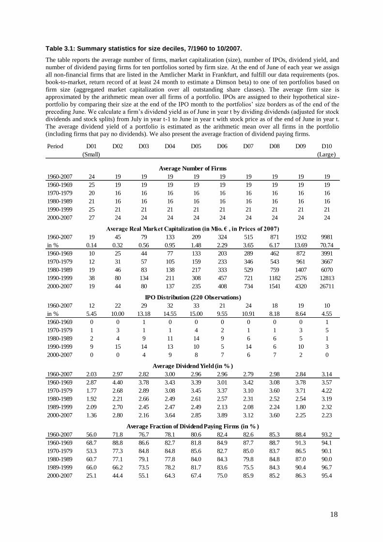
Table 3.1 shows that the average number of firms per size decile portfolio decreases from 19
in 1960 to 16 in 1990. From 1990 to 2007, the number of firms per decile increases from 16 to
24 on average.41 The number of firms per decile is relatively low compared to studies for the
U.S. market where deciles usually contain more than 100 firms.42 This has to be considered in
empirical tests, where we usually assume portfolios to be well diversified. Table 3.1 also
reports that the market capitalization of the firms included in the portfolio of the largest firms
is on average €9,981 mln. (in real terms based on the price levels of 2007), whereas the
market capitalization of the smallest is on average only €19 mln. (also in real terms) from
1960 to 2007. The decile portfolio of the largest firms, labeled D10, accounts on average for
ca. 70.7% of the total market capitalization of the Amtlicher Markt in Frankfurt (based on
equal-weight portfolios), whereas, the firms in the first six deciles represent together only
5.7% of the total market capitalization.
39
In later sections we sort by size, book-to-market, and beta. We also form two-dimensional sorted portfolios
sorting by these criterions. 40
We use the full time period of a firm’s exchange listing. Artmann/Finter/Kempf/Koch/Theissen (2012, p. 23)
“include only one class per firm in the sample and use the class for which the longer data history is
available.” 41
The sample size of Artmann/Finter/Kempf/Koch/Theissen (2012) increases more dramatically from 1990 to
2007. This is, because they also include lower market segments such as the Neuer Markt and the Geregelter
Markt in Frankfurt. 42
See for example Fama/French (1992), p. 436.
18
Table 3.1: Summary statistics for size deciles, 7/1960 to 10/2007.
The table reports the average number of firms, market capitalization (size), number of IPOs, dividend yield, and
number of dividend paying firms for ten portfolios sorted by firm size. At the end of June of each year we assign
all non-financial firms that are listed in the Amtlicher Markt in Frankfurt, and fulfill our data requirements (pos.
book-to-market, return record of at least 24 month to estimate a Dimson beta) to one of ten portfolios based on
firm size (aggregated market capitalization over all outstanding share classes). The average firm size is
approximated by the arithmetic mean over all firms of a portfolio. IPOs are assigned to their hypothetical size-
portfolio by comparing their size at the end of the IPO month to the portfolios’ size borders as of the end of the
preceding June. We calculate a firm’s dividend yield as of June in year t by dividing dividends (adjusted for stock
dividends and stock splits) from July in year t-1 to June in year t with stock price as of the end of June in year t.
The average dividend yield of a portfolio is estimated as the arithmetic mean over all firms in the portfolio
(including firms that pay no dividends). We also present the average fraction of dividend paying firms.
Period D01
(Small)
D02 D03 D04 D05 D06 D07 D08 D09 D10
(Large)
1960-2007 24 19 19 19 19 19 19 19 19 19
1960-1969 25 19 19 19 19 19 19 19 19 19
1970-1979 20 16 16 16 16 16 16 16 16 16
1980-1989 21 16 16 16 16 16 16 16 16 16
1990-1999 25 21 21 21 21 21 21 21 21 21
2000-2007 27 24 24 24 24 24 24 24 24 24
1960-2007 19 45 79 133 209 324 515 871 1932 9981
in % 0.14 0.32 0.56 0.95 1.48 2.29 3.65 6.17 13.69 70.74
1960-1969 10 25 44 77 133 203 289 462 872 3991
1970-1979 12 31 57 105 159 233 346 543 961 3667
1980-1989 19 46 83 138 217 333 529 759 1407 6070
1990-1999 38 80 134 211 308 457 721 1182 2576 12813
2000-2007 19 44 80 137 235 408 734 1541 4320 26711
1960-2007 12 22 29 32 33 21 24 18 19 10
in % 5.45 10.00 13.18 14.55 15.00 9.55 10.91 8.18 8.64 4.55
1960-1969 0 0 1 0 0 0 0 0 0 1
1970-1979 1 3 1 1 4 2 1 1 3 5
1980-1989 2 4 9 11 14 9 6 6 5 1
1990-1999 9 15 14 13 10 5 14 6 10 3
2000-2007 0 0 4 9 8 7 6 7 2 0
1960-2007 2.03 2.97 2.82 3.00 2.96 2.96 2.79 2.98 2.84 3.14
1960-1969 2.87 4.40 3.78 3.43 3.39 3.01 3.42 3.08 3.78 3.57
1970-1979 1.77 2.68 2.89 3.08 3.45 3.37 3.10 3.60 3.71 4.22
1980-1989 1.92 2.21 2.66 2.49 2.61 2.57 2.31 2.52 2.54 3.19
1989-1999 2.09 2.70 2.45 2.47 2.49 2.13 2.08 2.24 1.80 2.32
2000-2007 1.36 2.80 2.16 3.64 2.85 3.89 3.12 3.60 2.25 2.23
1960-2007 56.0 71.8 76.7 78.1 80.6 82.4 82.6 85.3 88.4 93.2
1960-1969 68.7 88.8 86.6 82.7 81.8 84.9 87.7 88.7 91.3 94.1
1970-1979 53.3 77.3 84.8 84.8 85.6 82.7 85.0 83.7 86.5 90.1
1980-1989 60.7 77.1 79.1 77.8 84.0 84.3 79.8 84.8 87.0 90.0
1989-1999 66.0 66.2 73.5 78.2 81.7 83.6 75.5 84.3 90.4 96.7
2000-2007 25.1 44.4 55.1 64.3 67.4 75.0 85.9 85.2 86.3 95.4
Average Number of Firms
Average Real Market Capitalization (in Mio. € , in Prices of 2007)
IPO Distribution (220 Observations)
Average Dividend Yield (in % )
Average Fraction of Dividend Paying Firms (in % )
19
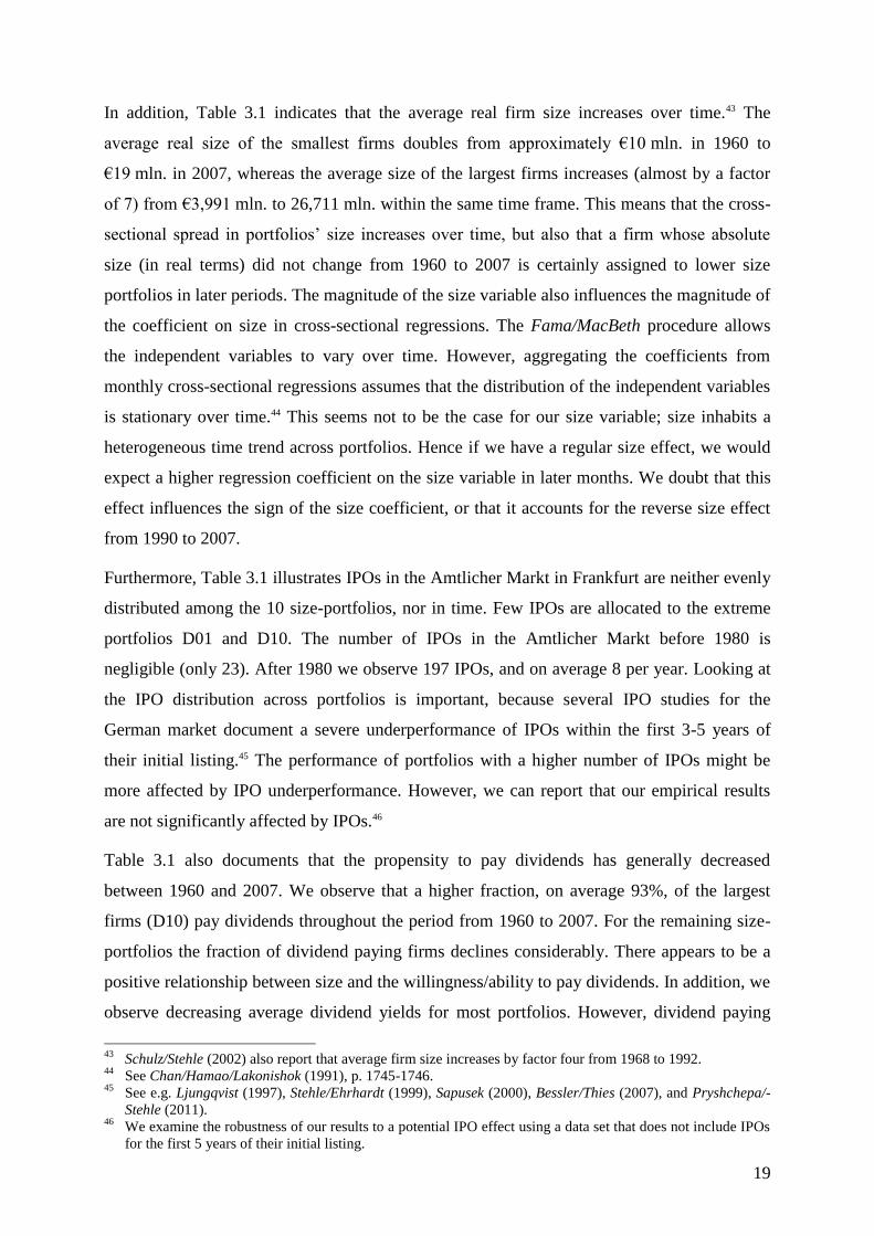
In addition, Table 3.1 indicates that the average real firm size increases over time.43 The
average real size of the smallest firms doubles from approximately €10 mln. in 1960 to
€19 mln. in 2007, whereas the average size of the largest firms increases (almost by a factor
of 7) from €3,991 mln. to 26,711 mln. within the same time frame. This means that the cross-
sectional spread in portfolios’ size increases over time, but also that a firm whose absolute
size (in real terms) did not change from 1960 to 2007 is certainly assigned to lower size
portfolios in later periods. The magnitude of the size variable also influences the magnitude of
the coefficient on size in cross-sectional regressions. The Fama/MacBeth procedure allows
the independent variables to vary over time. However, aggregating the coefficients from
monthly cross-sectional regressions assumes that the distribution of the independent variables
is stationary over time.44 This seems not to be the case for our size variable; size inhabits a
heterogeneous time trend across portfolios. Hence if we have a regular size effect, we would
expect a higher regression coefficient on the size variable in later months. We doubt that this
effect influences the sign of the size coefficient, or that it accounts for the reverse size effect
from 1990 to 2007.
Furthermore, Table 3.1 illustrates IPOs in the Amtlicher Markt in Frankfurt are neither evenly
distributed among the 10 size-portfolios, nor in time. Few IPOs are allocated to the extreme
portfolios D01 and D10. The number of IPOs in the Amtlicher Markt before 1980 is
negligible (only 23). After 1980 we observe 197 IPOs, and on average 8 per year. Looking at
the IPO distribution across portfolios is important, because several IPO studies for the
German market document a severe underperformance of IPOs within the first 3-5 years of
their initial listing.45 The performance of portfolios with a higher number of IPOs might be
more affected by IPO underperformance. However, we can report that our empirical results
are not significantly affected by IPOs.46
Table 3.1 also documents that the propensity to pay dividends has generally decreased
between 1960 and 2007. We observe that a higher fraction, on average 93%, of the largest
firms (D10) pay dividends throughout the period from 1960 to 2007. For the remaining size-
portfolios the fraction of dividend paying firms declines considerably. There appears to be a
positive relationship between size and the willingness/ability to pay dividends. In addition, we
observe decreasing average dividend yields for most portfolios. However, dividend paying
43
Schulz/Stehle (2002) also report that average firm size increases by factor four from 1968 to 1992. 44
See Chan/Hamao/Lakonishok (1991), p. 1745-1746. 45
See e.g. Ljungqvist (1997), Stehle/Ehrhardt (1999), Sapusek (2000), Bessler/Thies (2007), and Pryshchepa/-
Stehle (2011). 46
We examine the robustness of our results to a potential IPO effect using a data set that does not include IPOs
for the first 5 years of their initial listing.

20
firms allocated to the small and medium size deciles, D01 to D08, actually increase their
dividend payments on average by 25%. The reported decline in dividend yields for small
firms in Table 3.1 mainly results from a decreasing fraction of firms that actually pay
dividends. The different fraction of dividend paying firms and dividend yield across decile
portfolios also point out that corporate income tax credits must be included in the rate of
return calculation. Ignoring these benefits to share holders would penalize the performance of
large firm deciles (higher fraction of dividend paying firms) compared to small firm deciles.
As a consequence of missing dividends and/or missing income tax credits the chance to find a
regular size effect increases.
3.2 Average returns for decile portfolios
The results presented in this section are based on Table 6.1, Panels A, B, and C presented in
6.2 of this paper. We start by looking at the monthly excess returns in the top line of Panel A
in order to see whether a size effect in raw returns exists. In the time period 1960 to 1990, the
(arithmetic) means of the monthly excess returns of the three decile portfolios of the largest
firms are around .20%, all other portfolios have mean excess returns higher than .33%. This
holds for equal-weight and value-weight portfolios and is fully in line with a (regular) size
effect in raw returns. Testing the null of flat or weakly increasing pattern in average returns
across size deciles with the monotonicity relationship (MR) test of Patton/Timmerman (2010),
we obtain p-values of .047 (comparing adjacent portfolios) and .186 (comparing all possible
pairs) for equal-weight and of .138 (comparing adjacent portfolios) and .076 (comparing all
possible pairs) for value-weight portfolios. Hence, there is some support for a regular size
effect in raw returns during 1960 to 1990.47 From 1990 to 2007, the five portfolios containing
the firms whose size is above the median all have mean returns higher than .43%, the
portfolio of the largest firms even has a mean return above .70%. The mean excess returns of
the five portfolios of firms whose size is below the median are much smaller, and some are
even negative. This suggests that a reverse size effect in raw returns may exist in this period.
Again equal-weight and value-weight mean returns are very similar, this is what we expect
when we sort on size. Testing the null of a flat or weak decreasing pattern in average portfolio
returns during the second sub-period yields p-values for both versions of the MR test that are
above .50 for equal-weight as well as value-weight portfolios. However, removing the
portfolio of the smallest firms, D01, changes the results dramatically. The p-values are then
47
Patton/Timmerman (2010), p. 609 argue that “[t]he adjacent pairs are sufficient for monotonicity to hold, but
considering all possible comparisons could lead to empirical gains.”
21
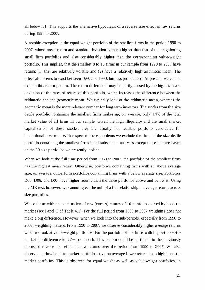
all below .01. This supports the alternative hypothesis of a reverse size effect in raw returns
during 1990 to 2007.
A notable exception is the equal-weight portfolio of the smallest firms in the period 1990 to
2007, whose mean return and standard deviation is much higher than that of the neighboring
small firm portfolios and also considerably higher than the corresponding value-weight
portfolio. This implies, that the smallest 8 to 10 firms in our sample from 1990 to 2007 have
returns (1) that are relatively volatile and (2) have a relatively high arithmetic mean. The
effect also seems to exist between 1960 and 1990, but less pronounced. At present, we cannot
explain this return pattern. The return differential may be partly caused by the high standard
deviation of the rates of return of this portfolio, which increases the difference between the
arithmetic and the geometric mean. We typically look at the arithmetic mean, whereas the
geometric mean is the more relevant number for long term investors. The stocks from the size
decile portfolio containing the smallest firms makes up, on average, only .14% of the total
market value of all firms in our sample. Given the high illiquidity and the small market
capitalization of these stocks, they are usually not feasible portfolio candidates for
institutional investors. With respect to these problems we exclude the firms in the size decile
portfolio containing the smallest firms in all subsequent analyses except those that are based
on the 10 size portfolios we presently look at.
When we look at the full time period from 1960 to 2007, the portfolio of the smallest firms
has the highest mean return. Otherwise, portfolios containing firms with an above average
size, on average, outperform portfolios containing firms with a below average size. Portfolios
D05, D06, and D07 have higher returns than the three portfolios above and below it. Using
the MR test, however, we cannot reject the null of a flat relationship in average returns across
size portfolios.
We continue with an examination of raw (excess) returns of 10 portfolios sorted by book-to-
market (see Panel C of Table 6.1). For the full period from 1960 to 2007 weighting does not
make a big difference. However, when we look into the sub-periods, especially from 1990 to
2007, weighting matters. From 1990 to 2007, we observe considerably higher average returns
when we look at value-weight portfolios. For the portfolio of the firms with highest book-to-
market the difference is .77% per month. This pattern could be attributed to the previously
discussed reverse size effect in raw returns over the period from 1990 to 2007. We also
observe that low book-to-market portfolios have on average lower returns than high book-to-
market portfolios. This is observed for equal-weight as well as value-weight portfolios, in
22
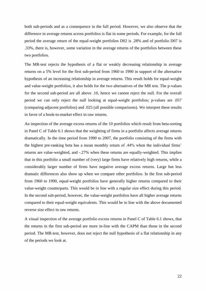
both sub-periods and as a consequence in the full period. However, we also observe that the
difference in average returns across portfolios is flat in some periods. For example, for the full
period the average return of the equal-weight portfolios D02 is .28% and of portfolio D07 is
.33%, there is, however, some variation in the average returns of the portfolios between these
two portfolios.
The MR-test rejects the hypothesis of a flat or weakly decreasing relationship in average
returns on a 5% level for the first sub-period from 1960 to 1990 in support of the alternative
hypothesis of an increasing relationship in average returns. This result holds for equal-weight
and value-weight portfolios, it also holds for the two alternatives of the MR test. The p-values
for the second sub-period are all above .10, hence we cannot reject the null. For the overall
period we can only reject the null looking at equal-weight portfolios; p-values are .057
(comparing adjacent portfolios) and .025 (all possible comparisons). We interpret these results
in favor of a book-to-market effect in raw returns.
An inspection of the average excess returns of the 10 portfolios which result from beta-sorting
in Panel C of Table 6.1 shows that the weighting of firms in a portfolio affects average returns
dramatically. In the time period from 1990 to 2007, the portfolio consisting of the firms with
the highest pre-ranking beta has a mean monthly return of .44% when the individual firms’
returns are value-weighted, and -.27% when these returns are equally-weighted. This implies
that in this portfolio a small number of (very) large firms have relatively high returns, while a
considerably larger number of firms have negative average excess returns. Large but less
dramatic differences also show up when we compare other portfolios. In the first sub-period
from 1960 to 1990, equal-weight portfolios have generally higher returns compared to their
value-weight counterparts. This would be in line with a regular size effect during this period.
In the second sub-period, however, the value-weight portfolios have all higher average returns
compared to their equal-weight equivalents. This would be in line with the above documented
reverse size effect in raw returns.
A visual inspection of the average portfolio excess returns in Panel C of Table 6.1 shows, that
the returns in the first sub-period are more in-line with the CAPM than those in the second
period. The MR-test, however, does not reject the null hypothesis of a flat relationship in any
of the periods we look at.

23
4 Major issues in applying the standard test procedures
4.1 Basic aspects of the standard test procedures
There has been a considerable progress in empirical tests of the CAPM since the first such
efforts in the sixties. Yet, to our knowledge, there is no general agreement with regard to the
proper test procedure. Therefore, we follow the most widely used procedures for testing linear
beta pricing hypotheses, the analysis of individual time-series regressions proposed by
Black/Jensen/Scholes (1972) [BJS], the cross-sectional regression procedure proposed by
Fama/MacBeth (1973) [FM] and the multivariate time-series regression test of
Gibbons/Ross/Shanken (1989) [GRS].48
Since the three procedures are based on different
assumptions and test objectives, and look at the time-series of cross-sectional data in different
ways, we consider them as ideal complements to each other, especially when the same set of
test portfolios are used, which we plan to do.
BJS tests examine whether the average returns of portfolios are in line with the CAPM (or a
competing model). Important assumptions of this procedure are:
a. We have a proper proxy for the market portfolio, that is (1), the composition of the
market portfolio is known, and (2), the data to measure/estimate the market portfolio’s
return is available. Roll (1977), in a widely quoted paper, argued that this is not the
case and discussed the serious consequences of not using a proper proxy.49
b. Based on equation (1) the test portfolios have stable alphas and betas during the test
period.
c. A risk-free asset exists.
d. The error terms from equation (1) are normally distributed, serially uncorrelated and
homoskedastic.
If the CAPM holds we expect BJS intercepts (also known as Jensen’s alpha), i , to be zero for
all test assets. An assumption about the functional form of the relationship between beta and
Jensen’s alpha is not required. This relationship could be linear or non-linear. Because of
infrequent trading issues we use a variation of the original BJS procedure, i.e. we estimate
48 All three procedures are discussed in detail in advanced text books such as Campbell/Lo/MacKinlay (1997),
Cochrane (2005), and Elton/Gruber/Brown/Goetzmann (2011). Recent review articles covering these tests
are Fama/French (2004), Subramanyam (2010), Jagannathan/Schaumburg/Zhou (2010) and Goyal (2012). 49
A proper proxy could be a portfolio that has the same return distribution and is perfectly correlated with the
true market portfolio.

24
portfolio intercepts from a model extended by the lagged market excess return when we use
monthly data:50
, , ,1 , , ,2 , 1 , ,i t f t i i m t f t i m t f t i tR R R R R R
(1)
where ,i tR is the rate of return of portfolio i during time interval t, ,f tR is the risk-free rate of
return, ,m tR is the return on the proxy for the market portfolio during period t, ,i t is the error
term of portfolio i in period t.51
BJS look only at the t-statistics of individual portfolios. An important result of the BJS test
could be that one or more portfolios have an economically or statistically significant non-zero
Jensen’s alpha. According to Gibbons/Ross/Shanken (1989) such a result is difficult to
interpret due to the contemporaneous cross-sectional dependence between the residuals of
different portfolios.52
They observe especially, that residuals of portfolios with similar betas
are positively correlated, those with very different betas are negatively correlated. Since the
alphas of the portfolios will inhabit the same pattern, it is difficult to conclude whether a
pattern in the alphas is due to correlation in the residuals or the true parameter.53
To overcome this problem we use the multivariate procedure of Gibbons/Ross/Shanken
(1989) [GRS] to test whether all intercepts are jointly equal to zero, that is, we use it as an
extension of the BJS tests. The GRS test does not require assumption (a) (we have a proper
market proxy). However, it requires assumptions (b) to (d) 54
, and in addition assumptions (e)
and (f):
e. The number of test assets is smaller than the number of time series observations55
;
f. The variance-covariance matrix of the residuals is stationary during the test period.
If assumption (a) (we use a proper proxy for the market portfolio) does not hold, the test tells
us, whether the proxy used is ex post mean-variance efficient when we use portfolios which
50 So far, we have not detected significant differences when we sort on beta and book-to-market using value-
weights. When we sort according to size, beta estimates differ. For quarterly and annual data we use the
standard procedure. 51
We adjust standard errors for heteroscedasticity and autocorrelation following Newey/West (1994) using an
automatic bandwidth selection procedure. 52
See Gibbons/Ross/Shanken (1989), p. 1130. 53
See Gibbons/Ross/Shanken (1989), p. 1138-1139. 54 In the absence of a risk-free asset, we could test the zero-beta version of the CAPM. In this case, however,
the null hypothesis is no longer linear in the parameters. Finally, we cannot apply the standard GRS test in
this case. See Gibbons/Ross/Shanken (1989, p. 1148). 55
The residual variance-covariance matrix has to be nonsingular. Usually N (the number of test assets to be
tested) is restricted by the number of observations T, whereas the choice of T is a question of stationarity.

25
were constructed on the basis of ex ante data to derive the efficient frontier. Under this aspect
the GRS-test is an ideal complement of BJS and FM.
A crucial question in the implementation of a BJS- or a GRS- test is the proper length of the
test periods. Using a longer test period increases the power of the test. It also increases the
probability that the stationarity assumptions (b), (d) and (f) are violated, which has
consequences for the test statistics and are difficult to evaluate. We will get back to this issue
in section 3.7 and 3.8. In view of the uncertainty about the proper length of the testing periods
we do BJS- and GRS-tests for 60 months, our two sub-periods, 7/1960 to 6/1990 and 7/1990
to 10/2007, and the full period from 7/1960 to 10/2007.
The FM procedure also requires assumptions (a), (proper proxy for the market portfolio).
Betas may vary over time, unless we use full period betas. However, the FM procedure
implicitly assumes that pre-ranking betas are informative for next period betas and that betas
are stationary during the period for which we estimate the pre-ranking beta and during the
subsequent test period. Several recent studies of the FM procedure focus on its power.
Grauer/Janmaat (2009) argue that the FM procedure lacks power to reject the null hypothesis
of a zero slope on beta.56
Murtazashvili/Vozlyublennaia (2012) conclude that the FM
procedure is less likely to reject the null if the CAPM almost holds, that is, if pricing errors
(alphas) are small, but negatively correlated with betas.57
Nevertheless, FM regressions may help us to identify anomalies, by including several
independent variables in the regression model. Like all linear regressions, FM assumes that
the relationship between the dependent and the independent variables is strictly linear. Our
full FM-regression model follows Fama/French (1992): it includes all three characteristics as
independent variables:
, , 1, , 2, , 3, , ,i t f t t t i t t i t t i t i tR R Size BM u
(2)
where ,i tR is the rate of return of portfolio/firm i during time interval t, ,f tR is the risk-free
rate of return, i is the intercept for period t, and ,i tu is the error term of portfolio/firm i in
period t.
The crucial difference between the FM procedure and more traditional cross-sectional
regression procedures is that the regression is ran for each period. The time series of
coefficients is used for hypothesis testing, that is, the time series of coefficients is used to
56 See Grauer/Janmaat (2009), p. 780.
57 See Murtazashvili/Vozlyublennaia (2012), p. 1057-1058.

26
calculate the average coefficients and the standard deviations of the average coefficients. This
has several advantages compared to traditional cross-sectional regression procedures:
Unbalanced panels do not create problems, betas may vary over time and, most importantly,
in any time period t the ,i tu ‘s may be cross-correlated.58
We also test variations of this model,
i. e. we use subsets of the independent variables in cross-sectional regressions.
Even though, the BJS, FM and GRS tests represent the most important basic test procedures,
the possible variations in these three procedures inhabit several problems. In the literature
these problems are usually examined one at a time. Finding an “optimal” test procedure is,
however, less apparent if several problems occur at the same time. The standard econometric
problems which complicate tests of the CAPM are the omitted variable problem, the unknown
true functional form of the relationship to be tested, serial autocorrelation, multicollinearity
and heteroscedasticity. In addition, problems occur which are related to the special nature of
the CAPM and the available data. The latter problems and their implications for our tests will
be discussed in the next sections:
should the tests be based on monthly, quarterly or annual data (section 4.2);
should we use data on individual firms or base our tests on portfolios (section 4.3);
how should we form the portfolios in the latter case (section 4.4);
should small and large firms be treated equally in our tests (section 4.5);
how should the betas be calculated (sections 4.6);
beta instability and its consequences for the test procedures (section 4.7);
the economic interpretation of the three test procedures (4.8).
We are aware of the fact that we cannot address all problems of CAPM tests. For example,
what we do not address are tests of conditional asset pricing models and (multi-) factor
models.59
4.2 Return interval
Most empirical tests of the CAPM are based on monthly rates of return. Some, as for example
Kothari/Shanken/Sloan (1995), Fama/French (1996) and Campbell/Vuolteenaho (2004),
58 Goyal (2012) discusses the differences between the traditional cross-sectional procedures and the FM
procedure in great detail, especially on page 13. 59
See Lewellen/Nagel/Shanken (2010) for a detailed discussion of factor model tests.

27
employ annual rates of return.60
Only a few studies, like Campbell/Vuolteenaho (2004) and
Avramov/Chordia (2006),61
employ quarterly data. Kothari/Shanken/Sloan provide three
reasonable arguments in favor of annual data: (1) the CAPM makes no assumption about the
investment horizon, (2) problems associated with low liquidity, and infrequent trading are less
severe, and (3) annual data mitigates problems related to anomalies such as the turn-of-the-
month (year) effect and the January effect. Even though annual data may reduce problems
related to seasonal effects, it cannot fully solve these problems.62
In addition, we expect fewer
problems to be caused by serial correlation for longer interval returns, especially with respect
to small firms.63
Stein (1996) provides an additional argument in favor of longer-horizon
returns. He argues that in an inefficient stock market, observed returns are subject to market-
wide noise. As a consequence of this pricing error, firms’ beta estimates will be biased.
However, in case of stationary market-wide noise the beta estimate will converge to *, the
unobserved beta given investors have rational expectation, if longer horizon returns are
employed.64
There is obviously a tradeoff between the mentioned effects and the larger amount of
observations associated with the use of monthly data, which we cannot quantify. We
alternatively use monthly, quarterly and annual return data in our empirical tests.
4.3 Individual firm vs. portfolio data
Studies that employ portfolio data in cross-sectional regressions use an argument introduced
by Miller/Scholes (1972): security betas cannot be observed, even if we have a proper proxy
for the market portfolio, but must be estimated, typically with historical rate of return time
series. The estimated beta may be interpreted as the sum of the true beta and an estimation or
60 Kothari/Shanken/Sloan (1995) use annual betas (from the regression of annual portfolio rates of return on an
equal-weight market portfolio) in their monthly FM regressions. 61
Avramov/Chordia (2006) employ quarterly data for testing a CCAPM due to the fact that consumption data is
available only on a quarterly basis. Most of their tests of the CAPM and the Fama-French 3 factor model are,
however, based on monthly data. 62
An alternative approach to account for the January effect would be simply to remove January observations or
to look at them separately as in as in Loughran (1997) and Stehle (1997). 63
Serial correlation in short interval returns yields downward biased risk estimates. This problem and possible
solutions have been discussed in the literature among others by Scholes/Williams (1977), Dimson (1979) and
Roll (1981). Looking at longer return intervals (monthly, quarterly, and annual) partly mitigates problems
with serial correlation. In section 4.6 we discuss the Dimson procedure, which accounts for serial correlation
and infrequent trading when estimating betas. 64
See Stein (1996), p. 445-447. Using a longer observation period (e.g. 25 years) with monthly data may also
solve the problem Stein describes. We are not aware of empirical evidence supporting the extent of Stein’s
basic argument.
28
measurement error.65
In a two-variable linear regression measurement errors in the
independent variable lead to downward biased (towards zero) estimate of its coefficient and
an upward biased (away from zero) estimate of the intercepts in cross-sectional regressions.66
The reduction of the bias caused by the measurement errors in the betas associated with the
use of portfolio data has been the major reason for using portfolio data, at least until the
1990s. The measurement error in betas decreases for sorts on betas, whereas groupings on
other criterions or random grouping of securities does not necessarily reduce the measurement
error in betas.67
To overcome the measurement error in the betas, securities (in our study firms) are usually
first grouped by the betas estimated on the basis of data (usually 60 months) preceding the
portfolio assignment date (pre-ranking betas). Next, the portfolio data for the subsequent test
period is analyzed econometrically; in a first step, the portfolio betas for the test period are
calculated (post ranking portfolio betas). Given that the measurement errors are imperfectly
correlated across securities within a portfolio, post-ranking portfolio betas are estimated more
precisely than individual security betas.68
However, it is also important that the measurement
errors in the pre-ranking betas and the post-ranking portfolio betas are uncorrelated.
Huang/Litzenberger (1988) point out that this assumption usually holds.69
Fama/French (1992) recognize the problem of measurement error in the beta. They argue that
beta estimation may be improved with portfolio data, but suggest to use individual firm data
(including the beta estimates based on portfolios) in the FM regressions.70
Ang/Liu/Schwarz
(2010) show that the procedure of Fama/French (1992) yields the same results as the
Fama/MacBeth (1973) procedure with equal-weight portfolios and beta as the only
independent variable.71
This we confirm in our empirical tests.72
Furthermore,
65 See Miller/Scholes (1972), p. 60–61 and Blume/Friend (1973), p. 23–26.
66 This is also pointed out by Black/Jensen/Scholes (1972), p. 84–85. Artmann/Finter/Kempf (2010) regress
securities rates of return on individual securities’ OLS betas in their cross-sectional analysis. We conclude,
that their beta estimates probably underestimate the systematic risk of most firms, especially of small firms.
Additionally, given the results of Black/Jensen/Scholes (1972), we expect their slope coefficients to be
downward biased. 67
See Black/Jensen/Scholes (1972), p. 118. 68
An alternative to grouping to reduce the measurement error has been advocated by Litzenberger/Ramaswamy
(1979). Instead of grouping securities by their beta they use the measurement error in beta to derive
consistent estimators (weighted least squares), that is, they put more weight on more reliable beta estimates in
the cross-section of security returns. 69
See Huang/Litzenberger (1988), p. 331. 70
See Fama/French (1992), p. 430-431. Another approach is taken by Brennan/Chordia/Subrahmanyam
(1998) who use risk adjusted rates of return of individual firms in FM regressions to overcome the
measurement error in betas. 71
See Ang/Liu/Schwarz (2010), p. 34.
29
Grauer/Janmaat (2004) argue that Fama/French (1992) regression results vary with the
applied sorting procedure; different results are obtained when portfolios are first sorted by
size and then by beta compared to sorting first by beta and then by size. We also observe
different cross-sectional results if we switch the sorting order.
To our knowledge, in empirical studies the univariate time-series test of BJS and the
multivariate time-series tests of GRS are only done on the basis of portfolio data.
Grouping may also be motivated by the associated reduction in the number of test assets,
which facilitates computations and the interpretation of the results. In addition, only a fraction
of firms exists over longer time periods. New stocks are introduced through IPOs, and
existing stocks are delisted because of acquisitions, mergers, bankruptcies and freeze-outs,
that is, our data set on individual firms is an unbalanced panel. Grouping generally mitigates
this (de-)listing problem and in addition smoothes extreme rates of return of individual
securities.73
Depending on the study design, the use of portfolios may allow the inclusion of a
specific firm during more time periods than in case of the use of data on individual firms. For
example, a security may be included immediately after the IPO when we form size portfolios.
When using data on individual firms, the rates of return on the IPO firm can only be included
once a return record of at least 24 months is available to calculate the beta of the firm. Also,
the assumption of stationary betas and expected excess rates of return over time is also more
likely fulfilled for grouped data than for individual securities. This is an important assumption
underlying the BJS and GRS tests, but also of the FM tests with full-period betas. Another
reason for the use of grouped data may simply be restricted access to firm data, whereas
portfolio data might be easily available to a researcher.74
72 In a world where there is no measurement error, Grauer/Janmaat (2004) point out that securities do not plot
along the security market line (as predicted by the Sharpe/Lintner CAPM) when equal-weight portfolio betas
are assigned to individual securities in the cross-section. They also note that the market portfolio is super-
efficient if equal-weight portfolio rates of return are employed. See Grauer/Janmaat (2004), p. 2903-2905.
They also discuss five problems of the Fama/French grouping procedure, which are related to GLS
regressions of rates of returns on beta. 73
See Blume/Friend (1973), p. 25-26. Since the standard estimators are based on the squared residuals, outliers
may have a large effect on the estimates. Alternatively, outliers could be winsorized or removed from the
sample. We carefully cross-checked all unusual observations/outliers. In addition, we primarily focus on
value-weight portfolios. Therefore, we neither remove nor winsorize returns or firms’ explanatory variables
as for example in Fama/French (1992) and Artmann/Finter/Kempf/Koch/Theissen (2012). However, even
winsorizing the top and bottom 5% affects our results only marginally. 74
French's data library (at http://mba.tuck.dartmouth.edu/pages/faculty/ken.french/data_library.html) provides
easy access to data for various portfolios, not only for the U.S. but also for many other countries. Portfolio
data for the German market is available from the website of the Centre for Financial Research Cologne
(CFR) (http://www.cfr-cologne.de).
30
If we group firms into portfolios, how should we do it? The choice of the grouping procedure
is typically based on the null hypothesis to be tested. In our context, the following H0-
hypotheses play a role:
- H0: the coefficient of beta is zero, that is, beta does not affect expected rates of return;
- H0: the CAPM holds exactly: all pricing errors are zero;
- H0: a size effect in raw returns does not exist (or book to market effect);
- H0: the CAPM holds and a size effect in risk-adjusted returns does not exist (or book-
to-market effect).
In addition the grouping procedures should not result in portfolios, which violate the
stationarity assumptions of the test procedure. For example, grouping by criterions other then
beta does not necessarily yield stationary portfolios betas.75
This is an aspect we think is very
important and, as a consequence, is carefully discussed in sections 4.7 and 4.8.
If beta is the only independent variable in a FM regression and the H0-hypothesis is “the
coefficient of beta is zero” where “beta does not affect the expected rate of return on assets”
then we should choose a grouping procedure that minimizes the measurement error in betas
and maximizes the dispersion of the betas across test assets. BJS (1972) were the first to
suggest to group securities by their betas in a prior time period.76
Fama/French (2004) and
Jagannathan/Schaumburg/Zhou (2010) conclude that this has become the standard procedure
since BJS. Lo/MacKinlay (1990) also argue in favor of the test procedures introduced by BJS
that is, sorts on beta.
Different grouping procedures are appropriate, when we test whether average returns are
related to anomaly variables such as firm size, book-to-market, and momentum,77
that is,
when we test the null hypotheses “the coefficient on size” and/or “the coefficient on book-to-
market” is zero.78
These indirect tests of the CAPM, therefore, typically group by the anomaly
75 Ang/Chen (2007), for example, show a remarkable variation in betas of portfolios sorted on book-to-market
across time. 76
Among others studies, Black (1993), Fama/French (1992), Kothari/Shanken/Sloan (1995) and Fama/French
(2004) also group securities by their beta. Several studies as for example Davis (1994) group securities into
portfolios by pre-ranking betas to estimate post-ranking portfolio betas which they assign to individual firms
as proposed by Fama/French (1992). Most studies do not just group by one criterion as for example by beta,
but also by other criterions. 77
French’s data library (http://mba.tuck.dartmouth.edu/pages/faculty/ken.french/data_library.html) contains
various portfolios, all sorted on anomaly variables like size, book-to-market, etc., none sorted on betas. 78
Another branch of the empirical literature started by Daniel/Titman (1997) test whether characteristic or
factor models explain stock returns. In these test securities are usually grouped by size and then by book-to-
market. Next, these groups are further subdivided according to firms’ factor loadings, HML or SMB,
resulting in three-dimensional grouping.

31
variables on which they focus.79
Since Fama/French (1993) sorting on size and then on book-
to-market (forming 5x5 portfolios) has become the most common grouping procedure.80
Also
note, whereas grouping by anomaly variables like size and book-to-market are solely induced
by empirical findings, grouping by beta is a theoretically grounded procedure.81
4.4 Problems of grouping
Huang/Litzenberger (1988) conclude “that grouping always results in a loss of efficiency.”82
Ang/Liu/Schwarz (2010) examine carefully whether individual securities or portfolios should
be used in cross-sectional tests. They warn that more precise estimates of betas for portfolios
do not necessarily translate into more precise estimates or lower standard errors of the
coefficients on beta.83
This problem is caused by a loss of information in the independent
variable (like beta, size, or book-to-market). Grouping reduces the cross-sectional dispersion
in the independent variable. As a consequence the standard error of the slope coefficient
increases, which decreases efficiency of slopes on portfolios compared to individual
securities. To minimize the loss of efficiency, groups must be formed in a way in which the
dispersion in the inter-group independent variables is maintained as much as possible.84
For
sorts on beta, the post-ranking portfolio betas should also approximately reproduce the sort of
the pre-ranking betas.
Another problem is that grouping by a variable that is subject to measurement error results in
groups that depend on the measurement error. Liang (2000) argues that grouping might
aggregate the measurement error of the variable used to form groups. Hence, it would be
unclear whether an independent variable adds to the cross-section of stock returns because of
a correlation between the variable itself or its measurement error with returns. As a
consequence, groups should be formed using a criterion that is independent of the
measurement error but highly correlated with the true value of the independent variable.
Lo/MacKinlay (1990) emphasize that grouping according to an empirically motivated
variable, like size, might yield misleading inferences. They refer to this problem as a data-
snooping bias. They conclude that the correlation between Jensen’s alpha and size in the U.S.
79 Among others Davis (1994), Davis/Fama/French (2000), and Ang/Chen (2007) group firms by book-to-
market. An overview of studies that sort by firms’ size is provided by Dijk (2011). 80
Among others this grouping procedure is applied by Fama/French (1993, 1996, 2005, 2011), Loughran
(1997), Davis/Fama/French (2000), Petkova/Zhang (2005), and Lewellen/Nagel (2006). 81
See Lo/MacKinlay (1990), p. 434. 82
See Huang/Litzenberger (1988), p. 330. 83
See Ang/Liu/Schwarz (2010), p. 26-27. 84
See Huang/Litzenberger (1988), p. 328-330.

32
might be a result of the correlation between size and the measurement error in alpha.
According to Lo/MacKinlay (1990) induced ordering will probably affect test statistics on
portfolios, whereas test statistics on individual securities are less affected. Our out of sample
tests based on size sorted portfolios are not subject to the data-snooping bias.85
Similarly, problems arise if the number of variables used to form groups is less than the
number of independent variables employed in the FM regression. A common example would
be the test of Fama/MacBeth (1973) where beta, the square of beta, and residual risk are
employed as independent variables in cross-sectional regressions on portfolios’ mean rates of
return. The test portfolios were solely grouped on firms’ betas, but not on firms’ residual risk.
The results of their empirical tests suggest that residual risk is not priced. However, this result
might be induced by the chosen sorting procedure and therefore just by chance. A common
procedure to overcome this problem is to group securities first by one variable and second to
subdivide the groups by another variable which results in dependent two-dimensional sorts.
Generally, groups should be formed taking all independent variables into consideration. The
main challenge here is restricted data availability, more groups translates into less securities
per portfolio and at some point portfolios might contain too few or no securities. Groupings
solely based on anomaly variables yield low inter portfolio spread in portfolio betas. As a
consequence, FM tests will lack efficiency with respect to the slope on beta.86
The choice of the number of test assets is also quite important. To elaborate, FM tests gain
efficiency for the slopes with an increasing number of portfolios. 87
Increasing the number of
portfolios results in less diversified portfolios and hence reduces regression fits.88
This also
affect the precision of intercepts in BJS time-series regressions. The GRS test requires,
because of non-singularity issues, that the number of test assets is considerably smaller than
the number of time series observations less the number of factors.89
The GRS test, however, is
more powerful if the number of portfolios is kept small. According to
85 See Lo/MacKinlay (1990), p. 461.
86 Grauer/Janmaat (2009), p. 786, referring to their Table 2, which shows betas for size and book-to-market
sorted portfolios, emphasize that grouping does not result in a wide range of betas, and hence cross-sectional
tests of whether the coefficient on beta is zero lacks power. Grauer/Janmaat (2009) also introduce an
interesting procedure to increase the spread in beta, and hence to increase the power of empirical tests. 87
Black/Jensen/Scholes (1972) form 10 portfolios, whereas Fama/MacBeth (1973), and Fama/French (1992)
form 12 portfolios, and Kothari/Shanken/Sloan (1995) form 20 portfolios in order to test the CAPM. 88
Our data set for the Amtlicher Markt in Frankfurt contains on average only 192 firms per year. Forming more
than 20 groups, thus results in groups with less than 10 firms per group, on average. 89
Gibbons/Ross/Shanken (1989, p. 1136) recommend that the number of test assets for which the variance-
covariance matrix is estimated, should be less than a third to one half of the number of time periods.

33
Campbell/Lo/MacKinlay (1997) GRS tests are more powerful if the number of groups is close
to 10.90
The power of the GRS test is also not invariant to the way we group securities.91
According to
Sentana (2009), Rada/Sentana (1997) suggest that the GRS test will have little power if
securities are grouped randomly. Sentana (2009) argues that this is caused by a low inter-
group variance in information ratios. Furthermore, he argues that grouping by firm
characteristics such as size and book-to-market produce disperse inter-group information
ratios, whereas industry groups have similar information ratios. Grouping procedures that
increase the inter-group information ratios increase the power of the test compared to
individual securities.92
4.5 Equal-weight vs. value-weight portfolios
The CAPM should generally hold for individual securities, as well as equal-weight and value-
weight portfolios. When we try to verify/reject it, a crucial question is: how should we
evaluate deviations of individual stocks/firms from the security market line (pricing errors)?
When we use data of individual firms or equal-weight portfolios with an identical number of
firms per portfolio, we implicitly assume that all individual deviations should be weighted
equally. In Germany, the largest firms are 1000 times as large as the smallest firms and have
stocks which are usually more liquid. When using value-weight portfolios, we implicitly
assume that the deviations associated with larger, that is economically more important firms,
should carry a larger weight than the deviations associated with smaller firms.93
In addition,
larger firms are rarely pure-play firms. Typically they consist of a parent company and
subsidiaries that is they are conglomerates. Equal-weight portfolios implicitly assign a smaller
weight to a firm if it operates as a subsidiary of a larger firm than to an otherwise identical,
but free-standing and exchange-listed firm.
An additional benefit of value weighting is that observations for which the probability that
they contain a data error is higher, receive a smaller weight. Even in a high quality data set,
data on dividends, stock splits and rights issues of small firms may be a little bit less accurate
90 See Campbell/Lo/MacKinlay (1997), p. 207
91 See Gibbons/Ross/Shanken (1989), p. 1137
92 See Sentana (2009), p. C77.
93 Buying stocks according to their market share would be an easy implementable and theoretically motivated
investment strategy. This strategy results in (market) value-weight portfolios. Alternatively an investor could
allocate his wealth across N stocks, where each stock represents 1/Nth of his portfolio. This portfolio must be
rebalanced at the beginning of each observation period, implying high transaction costs. This strategy also
implies buying past losers and selling past winners.
34
than the data on large firms. More important, as we will elaborate in section 4.6, betas for
small firms and/or portfolios of small firms are generally underestimated because of
infrequent trading and low liquidity.
A related question, especially for sorts on size, is: should we assign an equal number of
observations to portfolios? If we assign a larger number of firms to portfolios of small firms,
this will decrease the implicit weight of the firms in those portfolios and as a consequence in
the empirical tests. In most studies on the US market, this is achieved by assigning AMEX
and NASDAQ securities to portfolios according to NYSE “breaking points”. In general,
AMEX and NASDAQ stocks have a relatively low market capitalization. Therefore, U.S.
small stock portfolios contain more stocks than large stock portfolios.94
We hesitate to include
stocks of other market segments or from other stock exchanges into our analysis, primarily
because in Germany a market segment effect may exist.
Using different weights for small and large firms may be desirable economically. The
standard econometric procedures do not provide easy ways to do this. To our knowledge, no
study based on individual firm data gives larger firms a greater weight than smaller firms.
Fama/French (1992) for example use individual firms in their cross-sectional regressions and
thus give extremely small firms the same weights as extremely large firms. It could be argued
that small stocks are given too much weight in their study and hence drive the results.95
We
also do regressions based on individual firm data, but for this reason, give the results only
limited weight when we arrive at our over-all conclusions.
Most studies on the cross-section of stock returns employ equally-weighted portfolio returns.
Exceptions we are aware of include Daniel/Titman (1997), Loughran (1997), Fama/French
(2004), Ang/Chen (2007), and Fama/French (2008). Two of these studies use equal-weight as
well as value-weight portfolios. Loughran (1997) analyzes the impact of small firms on the
book-to-market effect and reports in his Table 5 that the spread between average returns of
high and low book-to-market quintiles drops from 6.23% for equal-weight portfolios to 3.93%
94 See for example Fama/French (1992), p. 430, and Daniel/Titman (1997), p. 31-32. Fama/French (2011), p. 6,
explain that this sorting procedure avoids sorts being dominated by small and less important, but plentiful
stocks. 95
Loughran (1997, p. 249) argues that the results of Fama/French (1992) are driven by “a January seasonal in
the book-to-market effect, and exceptionally low returns on small, young, growth stocks.”
Kothari/Shanken/Sloan (1995) argue that the results by Fama/French (1992) are exaggerated by a
survivorship bias in the COMPUSTAT data. However, Chan/Jegadeesh/Lakonishok (1995), Fama/French
(1996), and Chou/Huang/Lin/Hsu (2009) point out that a survivorship bias cannot and does not affect the
relationship between average rates of return and the book-to-market ratio for U.S. securities.
35
for value-weight portfolios. 96
Fama/French (2008) subdivide a sample of all firms from the
NYSE-Amex-NASDAQ universe into micro, small and big firm portfolios. For each of these
portfolios they estimate equal-weighted and value-weighted returns. In Table 2, they report
that the differences between those returns are generally largest within the micro firm
portfolio.97
In some cases the differences are even quite substantial within large firm
portfolios. Hence, we would expect regression results to vary with the weighting procedure,
even for a size group. Blume/Friend (1973) argue that value-weighted returns are
conceptually preferable to equal-weighted returns. However, they also warn that regression
estimators from value-weight portfolios may be less efficient and probably more subject to
measurement errors in the independent variables. This problem generally depends on the
portfolio composition. In Germany, the independent variables of value-weight portfolios are
dominated by a few large firms, especially if we do not sort on size. Hence, the portfolio beta,
and especially its measurement error, is dominated by a few large firms. Later we show that
the betas of large firms are measured more precisely, hence benefiting the portfolio betas.
Grauer/Janmaat (2004) warn that in a world without measurement error the CAPM might
appear correct, even though it is false when value-weighted portfolio rates of return are
employed.
We want to emphasize another problem which is also closely related to our above discussion
of individual vs. portfolio data especially with respect to our data set for Germany. We
observe for groups on firm size, that the market capitalization of the largest firms is on
average €10 bln. (in real terms), whereas the market capitalization of the smallest firms is on
average only € 19 mln. (in real terms) from 1960 to 2007 (see Table 3.1). Decile D10, which
includes the largest firms, represents on average 70% of the overall market capitalization of
the Amtlicher Markt, whereas, deciles D01 to D06 represent together less than 10%. Similar
observations have been made for the U.S. for example by Loughran (1997) and Fama/French
(2008).98
This means that approximately 10% of the overall market capitalization of the
Amtlicher Markt is implicitly assigned a weight of roughly 60% in cross-sectional regression
96 Loughran (1997) finds FM regression results on size and book-to-market to vary across NYSE, Amex and
NASDAQ firms. He observes a significant book-to-market effect for NYSE stocks in January only, whereas
for Amex and NASDAQ firms the effect appears outside January only. See Loughran (1997), table 6, p. 260. 97
Fama/French (2008), p. 1661, argue that there is a size effect within the micro firms, whereas tinier firms
have higher average returns. They also argue, based on the observation that EW and VW returns within small
and big firm portfolios are similar, and that the size effect is weaker for those firms. 98
Loughran (1997) reports that his largest size quintile represents on average 73% of the total market
capitalization during 1963 to 1995. See Loughran (1997), p. 250. Fama/French (2008), p. 1654 and p. 1656,
state that micro caps represent ca. 3% of the market cap of the NYSE-Amex-NASDAQ universe, whereas
they account for more than 60% of the firms during 1963 and 2005.
36
analyses based on individual firms or size sorted portfolios. As a consequence, regressions
estimated on all firms are heavily dominated by small firms. This is an important issue since
anomaly returns might not be pervasive across size groups, but only within certain groups.99
Loughran (1997), for example, argues that book-to-market does not explain returns of large
stocks.100
Fama/French (2008) estimate separate regressions for microcaps, small stocks, and
big stocks. They conclude that the size effect is more pronounced for microcaps, whereas
returns associated with book-to-market are more consistent across size groups.101
Our data set also contains many stocks with a market capitalization of less than €100 mln.
(see Table 3.1). OLS beta estimates of small stocks are generally systematically downward
biased as indicated below. We doubt that the Dimson procedure fully accounts for this
measurement error. Hence, the assumption that measurement errors are imperfectly correlated
across securities within a group is certainly violated. Small stocks, especially those with low
free-float, are also more subject to unusual return patterns. These unusual patterns usually
affect returns of equal-weight portfolios (unless portfolios contain many securities), even
though they are difficult to exploit by an investor.
Another aspect which we need to address is how we estimate the independent variables of
portfolios’ characteristics like size and book-to-market?102
We are currently not aware of any
paper that addresses this issue. We are not sure if all papers that use value-weight portfolios
also apply value-weighted size and book-to-market ratios as independent variables.103
However, the size effect hypothesizes a negative relationship between firm size and average
returns. The book-to-market effect describes a positive relationship between a firm’s book-to-
market ratio and its return. A portfolio’s independent variable must be estimated according to
its dependent variable, i.e. when we look at value-weight portfolios we should also estimate
portfolios’ value-weighted independent variables. To elaborate on the intuition behind this
argument we assume a portfolio that consist of few very large firms and many very small
firms. At first glance this seems to be a rather extreme and unrealistic situation, however, such
99 According to Fama/French (2008), p. 1654, U.S. small firms tend to have more extreme values of the
explanatory variables and more extreme rates of return. 100
See Loughran (1997), p. 250. 101
See Fama/French (2008), p. 1667-1669. 102
Note, betas are estimated regressing a portfolios equal-/value-weighted return on the market portfolio’s
return. Hence, equal-weight portfolios yield equal-weighted and value-weight portfolios value-weighted
betas. 103
We estimate portfolios’ value-weighted size and book-to-market ratios as Daniel/Titman (1997). They
describe in table IV a way to estimate value-weighted size and book-to-market ratios for portfolios. However,
since they focus on time-series regressions, they do not employ them as independent variables in cross-
sectional regressions. In appendix 6.1, we explain how we estimate the independent variables in more detail.
37
situations are actually quite plausible for Germany, especially when firms are sorted by their
pre-ranking betas and book-to-market ratios. The value-weighted return of this portfolio is
certainly dominated by the large firms, whereas the equal-weighted independent variable as
for example firm-size of that value-weight portfolio is dominated by the small firms. As a
consequence, we would try to establish a relation between the returns of large firms with a
size variable which is dominated by small firms. This would be in clear contradiction to the
definition of the size effect and could affect the regression coefficient in an arbitrary manner.
We follow Kothari/Shanken/Sloan (1995) when we calculate the natural log of the average
independent variables size and book-to-market.104
We address issues related to small firms placing less weight on those firms, simply by
employing value-weight portfolios. We also analyze equal-weight portfolios to check whether
our value-weight results are robust.
4.6 OLS vs. Dimson betas
Obviously, firm size and trading activity are highly correlated (whereas small firms are
usually less frequently traded).105
Roll (1981) concludes that because of positively serially
correlated returns, risk measures like beta and standard deviation obtained from short interval
return data seriously underestimate the actual risk of small sized firms.106
This makes it
difficult to compare risk adjusted rates of return across different sized firms, since
performance measures as Jensen’s alpha, the Treynor ratio and the Sharpe ratio are probably
overestimated for small sized firms, especially if they are obtained from short interval returns.
Note that serial correlation is not only a problem in daily, but also in monthly returns. We
observe decreasing serial correlation, indicated by variance ratios, for our size sorted
portfolios (not reported).107
Returns from one-dimensional sorts on beta and book-to-market
are also subject to this issue. This is an important issue in Germany since Table 3.1 indicates
that most German firms are tiny in terms of market capitalization. OLS beta estimates might
severely underestimate the systematic risk of these firms. Using systematically downward
104 See Kothari/Shanken/Sloan (1995), p. 193.
105 See James/Edmister (1983), p. 1075.
106 See Roll (1981), p. 879–883. Roll suggests that the underestimation of risk measures for small firms has the
potential to explain the firm size effect. However, Reinganum (1982) concludes that parts but not all of the
firm size effect can be explained by underestimated risk measures. See Reinganum (1982), p. 35. 107
If stock returns follow a random walk, the annual standard deviation should be about times the monthly
standard deviation. We calculate variance ratios dividing the variance from annual returns by the annualized
variance of monthly returns. For a detailed discussion on this topic see Lo/MacKinlay (1988), which provide
also a variance ratio test procedure.
38
biased OLS portfolio betas as independent variable in FM regressions yields biased slopes on
these betas. The classical errors-in-variables problem assumes that the measurement error is
uncorrelated with the unobserved variable, the true portfolio beta. Table 4.1 shows that the
difference between OLS and Dimson betas increases in betas. This suggests that the
measurement error in OLS betas is not entirely random. In case the measurement error is
positively correlated with the true beta, i.e. we assume the Dimson beta is a better estimate of
the true beta, the slope on beta will be biased away from zero.
Fama/French (1992) address this issue by estimating firms’ pre-ranking sum betas, according
to the procedure proposed by Dimson (1979). They regress firms’ rates of return on the
current and one-period lagged market return using 24 to 60 (as available) monthly
observations. They show for size-sorted portfolios that the difference between monthly post-
ranking OLS betas (simple betas) and Dimson betas increases from -0.03 (largest stocks) to
0.31 (smallest stocks) as firm size decreases.108
We generally estimate pre-ranking and full-
period Dimson betas following Fama/French (1992, 1996). Betas of firms that have multiple
share classes listed in the Amtlicher Markt at the same time are estimated using value-
weighted rates of return over all share classes of that firm.
McInish/Wood (1986) suggest that the Dimson estimator does not fully adjust for the beta bias
due to infrequent trading. Kothari/Shanken/Sloan (1995) propose to use OLS betas from
annual return interval in monthly cross-sectional regressions to overcome the thin trading
problems. In comparison to Fama/French (1992) they reveal a stronger positive relationship
between annual betas and average returns. However, Fama/French (1996) argue that these
results are probably attributed to an equal-weighted (which is probably not --efficient)
instead of a value-weighted proxy for the market portfolio.109
Nevertheless, we also employ
annual betas as part of our robustness checks. There are at least two more problems with
respect to beta estimates. First, if the market portfolio is not efficient, beta might not represent
a good measure of a firm’s systematic risk at all. Second, in section 4.7 we discuss in detail
that changes in the betas of small firm portfolios and large firm portfolios are generally
negatively correlated. This means, small changes in the average betas of large firms go
together with large changes in the average betas of small firms.
108 See Fama/French (1992), p. 431 and p. 454-455. We observe similar results for German firms (not reported).
109 See Fama/French (1996), p. 1952, Grauer (1999), p. 782.
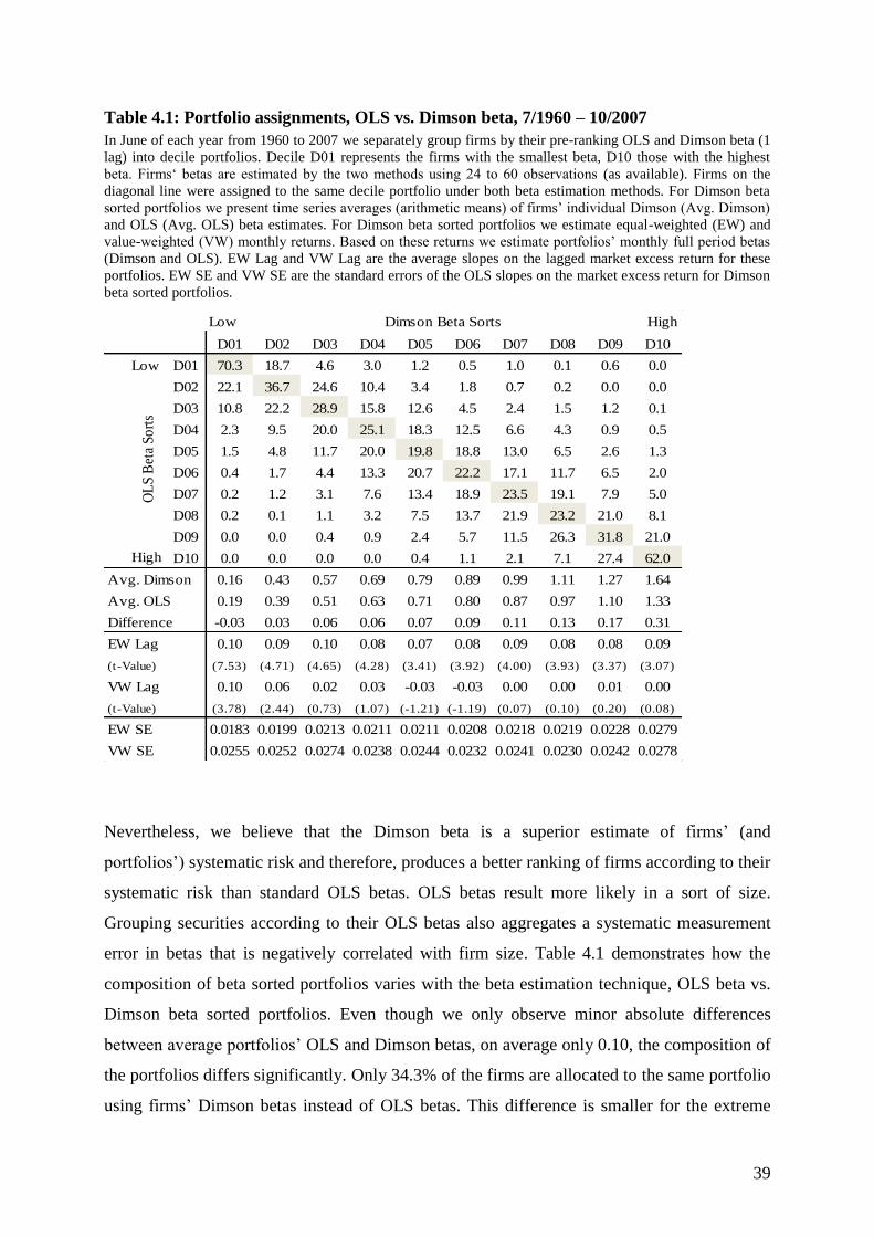
39
Nevertheless, we believe that the Dimson beta is a superior estimate of firms’ (and
portfolios’) systematic risk and therefore, produces a better ranking of firms according to their
systematic risk than standard OLS betas. OLS betas result more likely in a sort of size.
Grouping securities according to their OLS betas also aggregates a systematic measurement
error in betas that is negatively correlated with firm size. Table 4.1 demonstrates how the
composition of beta sorted portfolios varies with the beta estimation technique, OLS beta vs.
Dimson beta sorted portfolios. Even though we only observe minor absolute differences
between average portfolios’ OLS and Dimson betas, on average only 0.10, the composition of
the portfolios differs significantly. Only 34.3% of the firms are allocated to the same portfolio
using firms’ Dimson betas instead of OLS betas. This difference is smaller for the extreme
Table 4.1: Portfolio assignments, OLS vs. Dimson beta, 7/1960 – 10/2007
In June of each year from 1960 to 2007 we separately group firms by their pre-ranking OLS and Dimson beta (1
lag) into decile portfolios. Decile D01 represents the firms with the smallest beta, D10 those with the highest
beta. Firms‘ betas are estimated by the two methods using 24 to 60 observations (as available). Firms on the
diagonal line were assigned to the same decile portfolio under both beta estimation methods. For Dimson beta
sorted portfolios we present time series averages (arithmetic means) of firms’ individual Dimson (Avg. Dimson)
and OLS (Avg. OLS) beta estimates. For Dimson beta sorted portfolios we estimate equal-weighted (EW) and
value-weighted (VW) monthly returns. Based on these returns we estimate portfolios’ monthly full period betas
(Dimson and OLS). EW Lag and VW Lag are the average slopes on the lagged market excess return for these
portfolios. EW SE and VW SE are the standard errors of the OLS slopes on the market excess return for Dimson
beta sorted portfolios.
Low High
D01 D02 D03 D04 D05 D06 D07 D08 D09 D10
Low D01 70.3 18.7 4.6 3.0 1.2 0.5 1.0 0.1 0.6 0.0
D02 22.1 36.7 24.6 10.4 3.4 1.8 0.7 0.2 0.0 0.0
D03 10.8 22.2 28.9 15.8 12.6 4.5 2.4 1.5 1.2 0.1
D04 2.3 9.5 20.0 25.1 18.3 12.5 6.6 4.3 0.9 0.5
D05 1.5 4.8 11.7 20.0 19.8 18.8 13.0 6.5 2.6 1.3
D06 0.4 1.7 4.4 13.3 20.7 22.2 17.1 11.7 6.5 2.0
D07 0.2 1.2 3.1 7.6 13.4 18.9 23.5 19.1 7.9 5.0
D08 0.2 0.1 1.1 3.2 7.5 13.7 21.9 23.2 21.0 8.1
D09 0.0 0.0 0.4 0.9 2.4 5.7 11.5 26.3 31.8 21.0
High D10 0.0 0.0 0.0 0.0 0.4 1.1 2.1 7.1 27.4 62.0
0.16 0.43 0.57 0.69 0.79 0.89 0.99 1.11 1.27 1.64
0.19 0.39 0.51 0.63 0.71 0.80 0.87 0.97 1.10 1.33
-0.03 0.03 0.06 0.06 0.07 0.09 0.11 0.13 0.17 0.31
0.10 0.09 0.10 0.08 0.07 0.08 0.09 0.08 0.08 0.09
(7.53) (4.71) (4.65) (4.28) (3.41) (3.92) (4.00) (3.93) (3.37) (3.07)
0.10 0.06 0.02 0.03 -0.03 -0.03 0.00 0.00 0.01 0.00
(3.78) (2.44) (0.73) (1.07) (-1.21) (-1.19) (0.07) (0.10) (0.20) (0.08)
0.0183 0.0199 0.0213 0.0211 0.0211 0.0208 0.0218 0.0219 0.0228 0.0279
0.0255 0.0252 0.0274 0.0238 0.0244 0.0232 0.0241 0.0230 0.0242 0.0278
Difference
Avg. OLS
Avg. Dimson
VW Lag
(t-Value)
EW Lag
EW SE
VW SE
OL
S B
eta
So
rts
Dimson Beta Sorts
(t-Value)
40
portfolios (lowest and highest betas). The Dimson betas are on average higher than the OLS
betas for all Dimson beta sorted portfolios.
We also observe that the coefficient on the lagged market excess return is positive and
statistically significant for all equal-weight portfolios (see Table 4.1). For value-weight
portfolios the coefficients are statistically significant only for the two lowest beta portfolios,
D01 and D02. This result is caused by the large number of small firms, which dominate the
returns of equal-weight portfolios and translates into downward biased OLS beta estimates.
Value-weight portfolio returns are less affected by this bias as indicated by the lower value of
the lagged coefficient. For the value-weight portfolios only the lagged coefficients for D01
and D02 are statistically significant, possibly because of the higher number of small firms
assigned to these portfolios. This is indicated by a lower average market capitalization for the
low beta portfolios compared to the other portfolios (see Table 3.1).
To sum up, results for equal-weight portfolios are usually driven by the relatively large
number of small firms. In addition, betas for small firms are subject to the aforementioned
infrequent trading issue. Even though we adopt the Dimson procedure to estimate sum betas
we possibly make errors assigning small firms to beta portfolios. Value-weight portfolios are
less affected by this issue. We assume that betas of large firms are measured more precisely.
This also benefits betas of value-weight portfolios, even though these estimates are dominated
by returns of a few large firms. Table 4.1 also indicates that the standard error of the
coefficient for our value-weight portfolios resembles the standard error of the coefficients of
our equal-weight portfolios. Analyzing value-weight portfolios is also more in line with
modern portfolio theory and has a stronger economic meaning. Inferences from equal-weight
portfolios are rather unreliable, even though equal-weight portfolios are more in line with
econometric theories.
4.7 Time varying portfolio betas
Figure 4.1 illustrates some interesting patterns in the variation of betas for size sorted
portfolios during the period from 1960 to 2007.110
The 5-yr post-ranking rolling Dimson beta
for the portfolio of the largest German firms (bottom graph in Figure 4.1, solid line) varies
within the rather narrow range of 0.87 (just before the subprime crisis) and 1.22 (just before
the dot-com bubble bursted). The range of the betas of the lower size portfolios is more than
110 The discussion of time varying betas starts with Blume (1971) and Baesel (1974), a recent study for German
stock data is Eisenbeiss/Kauermann/Semmler (2007).
41
twice as large, it is from 0.31 to 1.15 for medium sized firms (D05) and from 0.25 to 1.19 for
the smallest firms (D01). This shows that in Germany (1) there is more variation in the betas
of small firms compared to large firms (this is generally in line with the U.S. market (top
graph in Figure 4.1)); (2) the betas of small firms are generally lower than those of large firms
(this is opposite to the U.S. market, where these betas are generally higher).111
In both markets
the inter-portfolio spread of the betas of the ten size portfolios also varies considerably over
time. In Germany, it ranges from .16 in September 1962 to .96 in November 2000. Also note
that the portfolios containing the smallest firms do not always have a lower beta than the
portfolio of the largest firms in Germany. Neither do the portfolios of the smallest firms
always have a higher beta than the portfolio of the largest firms in the U.S.
The value-weighted sum of all size portfolios’ betas plus the beta of the financials should be
unity on average. This implies that typically small changes in the betas of the largest firms go
together with large changes in the betas of the smallest firms in the opposite direction. Figure
4.1 illustrates this relationship for the U.S. market using Ken French’s value-weighted size
sorted portfolios. From July 1962 to July 1970, the beta of the portfolio of the largest U.S.
firms decreased nearly continuously by a total of 8% (from 1.00 to .92). In the same time
interval, the beta of the portfolio of the smallest firms almost doubled from 1.16 to 1.94. From
July to November 1974, the beta of the portfolio of the largest firms increased by .05, and the
beta of the portfolio of the smallest firms decreased by -.36. A major source for the variation
in portfolios’ and firms’ betas over time is simply induced by the constitution of the proxy for
the market portfolio and the mechanics of beta estimation. As a consequence of the variation
in portfolios’ betas, results from the BJS and GRS test for size portfolios need to be
interpreted with caution. Both test procedures implicitly assume portfolio betas to be
stationary over time. A common procedure to address this issue is to subdivide the sample
into five year intervals assuming that betas are stationary over this shorter time period.112
Another noteworthy aspect in Figure 4.1 is the beta of the portfolio of financial firms which
consists largely of Germany’s exchange listed universal banks and insurance companies.
Typically (and especially since 2003) these firms have the highest betas. Also note that
financial firms are represented by the proxy for our market portfolio, but not by our test
portfolios.
111 Studies for the US market revealed an inverse relationship between firm size and beta, i.e. portfolios’ post-
ranking betas are decreasing in average portfolio size. See Fama/French (1992), Kothari/Shanken/Sloan
(1995). 112
See Gibbons/Ross/Shanken (1989), p. 1132-1133.
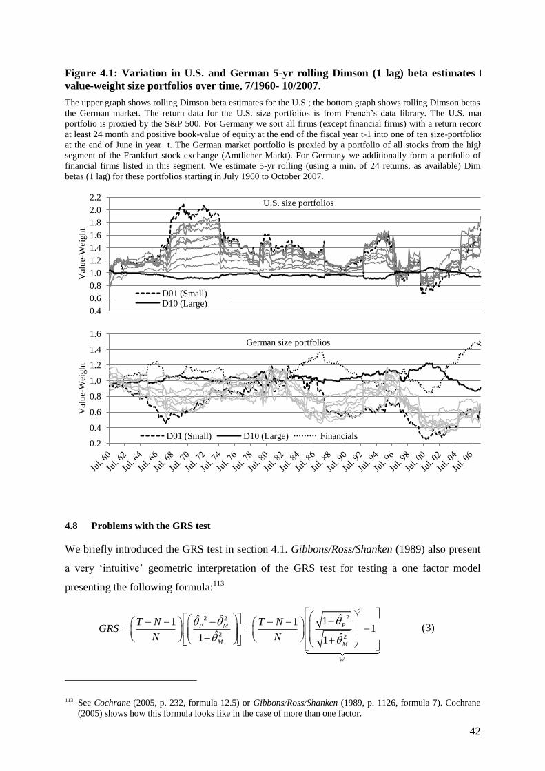
42
4.8 Problems with the GRS test
We briefly introduced the GRS test in section 4.1. Gibbons/Ross/Shanken (1989) also present
a very ‘intuitive’ geometric interpretation of the GRS test for testing a one factor model
presenting the following formula:113
222 2
2 2
ˆˆ ˆ 11 11
ˆ ˆ1 1
PP M
M M
W
T N T NGRS
N N
(3)
113 See Cochrane (2005, p. 232, formula 12.5) or Gibbons/Ross/Shanken (1989, p. 1126, formula 7). Cochrane
(2005) shows how this formula looks like in the case of more than one factor.
Figure 4.1: Variation in U.S. and German 5-yr rolling Dimson (1 lag) beta estimates for
value-weight size portfolios over time, 7/1960- 10/2007.
The upper graph shows rolling Dimson beta estimates for the U.S.; the bottom graph shows rolling Dimson betas for
the German market. The return data for the U.S. size portfolios is from French’s data library. The U.S. market
portfolio is proxied by the S&P 500. For Germany we sort all firms (except financial firms) with a return record of
at least 24 month and positive book-value of equity at the end of the fiscal year t-1 into one of ten size-portfolios as
at the end of June in year t. The German market portfolio is proxied by a portfolio of all stocks from the highest
segment of the Frankfurt stock exchange (Amtlicher Markt). For Germany we additionally form a portfolio of all
financial firms listed in this segment. We estimate 5-yr rolling (using a min. of 24 returns, as available) Dimson
betas (1 lag) for these portfolios starting in July 1960 to October 2007.
0.4
0.6
0.8
1.0
1.2
1.4
1.6
1.8
2.0
2.2
Val
ue-
Wei
ght
D01 (Small) D10 (Large)
U.S. size portfolios
0.2
0.4
0.6
0.8
1.0
1.2
1.4
1.6
Val
ue-
Wei
ght
D01 (Small) D10 (Large) Financials
German size portfolios

43
where denotes the Sharpe ratio of the market portfolio, M; denotes the Sharpe ratio of
the optimal ex post tangency portfolio, a combination of all test portfolios and M. This implies
that . Under the null hypothesis both Sharpe ratios do not differ considerably, so that
W, the term in square brackets in equation (3) would be close to zero. The larger the
difference between these two Sharpe ratios the more likely the GRS test rejects the null.
We find the maximum ex post Sharpe ratio of the tangency portfolio solving a classical
portfolio optimization problem. The input parameters to this problem are the returns of the N
test portfolios, the market portfolio M, and the risk-free asset as well as the combined
covariance matrix of the N test assets and M. Solving this optimization problem yields
insights into the implied composition of P implied by the GRS test. Implicitly, the GRS test
makes no assumption regarding short positions in P.114
In addition to P, we construct a
portfolio PnS under the assumption that short sales are not allowed.115
In Figure 6.1, we
present the solution to these optimization problems using our size decile portfolios.
For the period from 1960 to 2007 the GRS test does not reject the CAPM, the p-value is
.2625. However, the implicit weights of most test portfolios to derive T are quite remarkable,
e.g. we would need to short the market portfolio by 140%. In addition, the annualized average
return of T from July 1960 to October 2007 is approximately 19%. Given an average risk-free
rate of 4% would yield a market risk premium of 15%, compared to 4% based on the market
portfolio. During the first sub-period from 1960 to 1990, where we observe a regular size-
effect, we weight the market portfolio with 18% only. We short the three portfolios containing
the largest firms (weights are -143%, -70% and -12% for the largest), which together
represent on average ca. 80% of the total market capitalization. However, based on the GRS
test, p-value of .3140, we cannot reject the CAPM. The GRS p-value for the second sub-
period from 1990 to 2007 is .0438, i.e. we can reject the CAPM on a 5% significance level.
The weights for most size portfolios are either very low, or very high. We would short the
market portfolio with -557%(!), as well as portfolio D2 (-799%!) and D3 (-681%!). The three
largest portfolio holdings with positive weights are D6 (608%), D10 (459%) and D8 (385%).
The resulting tangency portfolio, P, has an average annualized rate of return of approximately
40%.
114 Solving this linear programming problem we assume a maximum investment of 10 times the initial
investment, that is, we allow the weights of the test assets to vary in a range between -1000% and +1000%. 115
First, we construct the mean-variance frontier. This is done by solving a quadratic optimization
(programming) problem with two linear constraints for a series of given rates of return. Second, we select the
portfolio which yields the maximum Sharpe ratio given the empirical risk-free rate of return. We call this
portfolio PnS (nS for no shorts).
44
These portfolio compositions are obviously not maintainable; the weights are unrealistic and
vary considerable over time. Assigning positive weights to the test assets and the market
portfolio to derive the tangency portfolios would probably be a more realistic assumption.
Under this assumption we trace out PnS weighting D6 with 51%, D8 with 26% and D10 with
23% for the second sub-period. The p-value of .9951 suggests that the difference between the
Sharpe ratio of the PnS and M is not statistically significant. However, the composition of the
tangency portfolio is not very encouraging; most portfolios including the market portfolio
have zero weights.116
We want to mention that the choice of the proxy for the risk free rate of return can influence
the results heavily as it is shown in Levy/Roll (2010).117
Increasing the risk free rate of return
(by using another proxy) could lead to even lower rejection rates when testing the efficiency
of our market proxy.118
Another problem is related to the assumption of normal i.i.d. residuals. GRS suggest applying
their F-test for five year intervals, because of stationarity concerns. We find many
applications of the GRS test in the literature for time periods of 30 years or even longer.119
Levy/Roll (2010) show that the GRS test cannot reject the CAPM for sample periods with less
than seven hundred months of data when they look at 12 U.S. industry portfolios for the
period from 1926 to 2008 and using a risk-free rate of .20%.120
For our aforementioned size-
sorted decile portfolios (as well as other sorts), however, we can easily reject the null
hypothesis that the residuals from the BJS regressions for the full period or the two sub-
periods are normal i.i.d. using standard test procedures. This is mainly due to the high
skewness and kurtosis of the residuals. Time varying portfolio betas additionally account for
heteroscedasticity in the residuals. Affleck-Graves/McDonald (1989) conclude that although
the GRS test is reasonably robust for minor deviations from normality, it can substantially
understate the actual significance level in case of large deviations from normality. As a
consequence of non-normality of the residuals the power of the GRS test will be overstated
116 Levy/Roll (2010) overcome this issue modifying the returns and variances of the test assets (within their
estimation error bounds), showing that the market portfolio can be efficient. 117
See Levy/Roll (2010), Figure 7 on page 2480. 118
We use the one month money market rates reported by Frankfurt banks as our proxy for the risk-free rate of
return throughout the paper. 119
The GRS test is applied for periods longer than 30 years among others by Fama/French (2006) for the period
7/1926 to 12/2004 (942 months) and two sub-periods, from 7/1926 to 6/1963 (444 months) and from 7/1963
to 12/2004 (498 months); Feguson/Shockley (2003) for 7/1964 to 12/2000; Fama/French (1996) for 7/1963
to 12/1993 (366 months). 120
See Levy/Roll (2010), p. 2480-2482. They also conclude that “the CAPM cannot be rejected when estimation
errors in the standard deviations are taken into account” looking at the entire period from 1926 to 2002 (990
months). For the same time period the GRS test rejects the CAPM with a p-value of .03.

45
and the p-values of the GRS test statistic will be too low.121
The bias increases with the level
of the non-normality in the residuals. This may account for low p-values in empirical tests,
and as a consequence increase the probability to mistakenly reject the null hypothesis. We
implement the GRS test for our full-period, 7/1960 to 10/2007, and the two sub-periods,
7/1960 to 6/1990 and 7/1990 to 10/2007, as well as non-overlapping five year intervals.
121 See Affleck-Graves/McDonald (1989), p. 897–898.
46
5 Results
We group securities by their pre-ranking beta to test the CAPM directly. Furthermore, we sort
on size, and book-to-market (one-dimensional sorts) to explore whether these two variables
are potential candidates of anomaly variables. We also highlight results for two-dimensional
sorts on size and book-to-market. For one-dimensional sorted portfolios we generally present
results for deciles, however, as part of our robustness checks we also form 16 and 20 one-
dimensional sorted portfolios. For two-dimensional sorts we primarily focus on 4 by 4 sorts,
however, we also check the robustness of our results looking at 2x2, 3x3, 5x5 and 6x6 sorts.
We also check whether empirical results depend on the sorting order, i.e. does sorting by size
and then by book-to-market yield different results as sorting first by book-to-market and
second by size? In addition, we do not only look at monthly return data, but also at quarterly
and annual return data. We use monthly, quarterly and annual full-period betas, but also
monthly and quarterly rolling betas as independent variables in our FM tests. We generally
stress results for value-weight portfolios, but also present results for equal-weight portfolios.
For value-weight portfolios we estimate value-weighted size and book-to-market variables.
We follow the same pattern for equal-weight portfolios. We look at the full time period from
1960 to 2007, but also at two sub-periods. The first sub-period extends from July 1960 to June
1990, the second from July 1990 to October 2007.
5.1 Results based on one-dimensional sorts
5.1.1 Sorts on firm size
In section 3.1 we focused on one-dimensional sorted size-portfolios to present the main
characteristics of the firms in our data set. In section 4 we illustrated that sorts on size also
inhabit several problems. (1) Cross-sectional results for sorts on size are dominated by small
firms. (2) The results for beta lack efficiency in cross-sectional FM tests. (3) The results for
book-to-market also lack efficiency. Thus it remains unclear whether a size effect prevails
once other independent variables are added to the model. (4) The betas of size portfolios have
undesirable properties. Nevertheless, many papers on the cross-section of stock returns
conduct empirical tests for size-sorted portfolios. There are several reasons supporting this
procedure. An important one is that the weighting of the intra portfolios’ rates of return has
least influence on the results. Another important reason is that it allows us to draw
conclusions about the existence of a market-wide size effect in raw returns.
Compared to the results (average returns) for size sorted portfolios in section 3.2 we obtain
even stronger results when we use FM cross-sectional regressions in which excess rate of
47
return is used as the dependent and size as the only independent variable (see Table 6.6). In
the first sub-period the coefficient on size (more exactly the natural logarithm of size) is
negative, but not significant in all of our 22 regressions with data sets which differ with
respect to weighting (equal weight vs. value weight portfolio returns), return interval
(monthly, quarterly and annual), number of portfolios and the inclusion of portfolio D01. In
the second sub-period the coefficient on size is always positive, economically very and
statistically highly significant in the 22 comparable FM regressions (reverse size effect). It is
mostly positive, but never significantly so in the overall period. The intercepts also have a
systematic pattern across the three observation periods: they are strongly positive
(economically and statistically significant) in the first sub period, negative, not quite as strong
in the second sub-period and slightly positive in the over-all period.
In the next step we run 44 FM regressions that include beta in addition to size as an
independent variable (results not shown). These regressions differ with respect to the number
of groups, the return intervals, and the way portfolio betas are estimated. Compared to only
using size as independent variable this changes the coefficients of size and the related t-values
in the following way: (1) In the first sub-period most coefficients remain practically the same.
There is a tendency, that in the regressions based on annual data the coefficients are a bit
more negative and their t-statistics a bit higher, for equal weight portfolios they are close to
being significant. When we employ rolling or annual full period beta estimates in the
regressions based on monthly or quarterly data, the t-values are typically higher and for equal-
weight portfolios often statistically significant. (2) In the second sub-period, the coefficient is
often a bit larger and generally highly statistically significant. (3) For the overall period most
FM test variations yield positive and statistically insignificant coefficients on size.
In these 44 FM regressions the coefficients on beta are typically positive in the sub-period
from 1960 to 1990, especially when we use annual data, betas based on annual data or rolling
betas. With these, the associated t-values are on average around 1. In the second sub-period
the coefficients on betas are typically negative, in the overall period they are mostly negative,
in both periods they are nearly always statistically insignificant.
When we include book-to-market in addition to size as an independent variable we observe in
22 FM regressions the following characteristics for the coefficients on size (results not
shown): (1) always negative, but not statistical significant in the first sub-period. (2) Always
positive, statistically significant in equal-weight portfolios, or if we increase the spread of the
size variable by forming 16 or 20 size portfolios instead of ten, in the second period. (3)

48
Positive, but insignificant in the overall period. The characteristics of the book-to-market
coefficients are the same in all three observation periods: (1) always positive and statistically
significant when we use twenty portfolios (2) positive but not significant if we use only 16 or
10 portfolios.
Adding both beta and the book-to-market in addition to size as independent variables does not
yield new insights on the size effect. In fact, because of the high correlation between size and
beta, and size and book-to-market we would expect higher standard errors of the estimated
coefficients as soon as we include more than one independent variable. We also do not sort by
beta or book-to-market, which results in low inter-portfolio spreads for these variables.
Nevertheless, even though we look at size sorted portfolios, the book-to-market effect
emerges in our data set and appears to be statistically significant in some variations of the test
procedure, especially as we increase the number of size sorted portfolios from ten to twenty.
We want to reiterate that the betas of our size sorted portfolios are not stationary (see Figure
5.1). We already discussed problems caused by this issue in section 4.7. Despite of the
problems caused by non-stationary betas, we proceed with BJS time-series tests where we
focus on Jensen’s alphas. We primarily conduct these tests for monthly excess returns of size
sorted decile portfolios. BJS allows us to identify the portfolios that deviate most from the
CAPM prediction for a specific period (see Panel A in Table 6.1). In the first sub-period
(1960-1990) when we look at either equal-weight or value-weight portfolios, we observe
negative or near neutral (annualized) Jensen’s alphas for the three largest size portfolios, and
positive for the seven portfolios containing smaller firms. Most t-values are not significant. In
the second sub-period (1990-2007) an even stronger reverse size effect prevails. The top five
deciles of the largest firms all have positive alphas; whereas the small firm portfolios, except
for the smallest firm decile, have negative alphas. Again, most t-values are not significant.
This effect is economically so strong, however, that we also observe a reverse size effect
within the full period. Here, none of the t-values are significant. As in the analysis of raw
returns, the results indicate, that size related effects are not stable within our overall sample
period.113
Again, the performance of portfolio D01 deviates considerably from its neighboring
portfolios: the annualized Jensen’s alpha is nearly 8% higher than that of portfolio D02.
113
Several authors document a reversal of the size effect. Dimson/Marsh (1999) report a reversal of the size
effect for the U.S. and the UK markets. Earlier studies on the size effect such as Blume/Friend (1974),
Brown/Kleidon/Marsh (1983) and Blume/Stambaugh (1983) also report that the size-effect is non-stationary
across sub-periods.
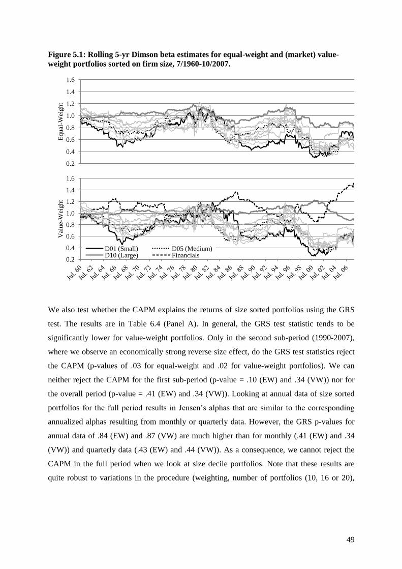
49
We also test whether the CAPM explains the returns of size sorted portfolios using the GRS
test. The results are in Table 6.4 (Panel A). In general, the GRS test statistic tends to be
significantly lower for value-weight portfolios. Only in the second sub-period (1990-2007),
where we observe an economically strong reverse size effect, do the GRS test statistics reject
the CAPM (p-values of .03 for equal-weight and .02 for value-weight portfolios). We can
neither reject the CAPM for the first sub-period (p-value = .10 (EW) and .34 (VW)) nor for
the overall period (p-value = .41 (EW) and .34 (VW)). Looking at annual data of size sorted
portfolios for the full period results in Jensen’s alphas that are similar to the corresponding
annualized alphas resulting from monthly or quarterly data. However, the GRS p-values for
annual data of .84 (EW) and .87 (VW) are much higher than for monthly (.41 (EW) and .34
(VW)) and quarterly data (.43 (EW) and .44 (VW)). As a consequence, we cannot reject the
CAPM in the full period when we look at size decile portfolios. Note that these results are
quite robust to variations in the procedure (weighting, number of portfolios (10, 16 or 20),
Figure 5.1: Rolling 5-yr Dimson beta estimates for equal-weight and (market) value-
weight portfolios sorted on firm size, 7/1960-10/2007.
0.2
0.4
0.6
0.8
1.0
1.2
1.4
1.6
Eq
ual
-Wei
ght
0.2
0.4
0.6
0.8
1.0
1.2
1.4
1.6
Val
ue-
Wei
ght
D01 (Small) D05 (Medium) D10 (Large) Financials
50
return interval (monthly, quarterly, annual). Also note that our decision to remove the
portfolio of the smallest firms, D01, does not influence the results for the GRS test much.114
Given the high skewness and kurtosis of the residuals, we can reject the null hypothesis that
the residuals from the BJS regressions are normal distributed. In the previous section we
argued based on the work of Affleck-Graves/McDonald (1989) that as a consequence of non-
normality in the residuals the power of the GRS test will be overstated and the p-values of the
GRS test statistic will be too low.115
The bias increases with the level of the non-normality of
the residuals. This may account for our low p-values for the second sub-period, where we
reject the null hypothesis that the CAPM holds on the 5% significance level. In other words,
the rejection of the CAPM in the second sub-period could be simply due to non-normal i.i.d.
residuals. Also note that the GRS results are sensitive to the number of portfolios, especially
for the second sub-period. Using 16 portfolios instead of 10 yields p-values of 0.05 (EW) and
0.11 (VW) for the GRS test, whereas 20 portfolios yield considerably lower p-values of 0.01
(EW) and 0.01 (VW).116
We address the problem induced by non-stationary portfolio betas (see Figure 5.1) dividing
the overall period into five year, non-overlapping intervals. For each interval we run the GRS
test. The results are in Table 7.5 (Panel A). Aggregating the GRS coefficients yields average
p-values well above .26 for our two sub-periods (1960-1990, and 1990-2007) as well as for
the overall period. This result is independent to the weighting scheme as well as the number
of portfolios (10, 16, 20). Only for the 5yr interval from 2000 to 2005 we observe p-values
that are generally below .05 and close to zero. For all other 5yr intervals the p-values are
usually above .10. This means that based on size sorted portfolios we could reject the CAPM
only for the period from 2000 to 2005.
Taken together, the FM analysis of the excess returns of the portfolios grouped on the basis of
size shows: (1) between 1960 and 1990 a moderate size effect in raw returns may exist,
between 1990 and 2007 an economically strong and statistically significant reverse size effect
in raw returns exists. (2) BJS and GRS tests do not support these results for the first sub-
period, but show clear signs for a reversed size effect in the second sub-period, especially
during the time period between 2000 and 2005. The results differ for the number of portfolios
114
The results for the GRS test only change considerably with respect to portfolio D01 when we look at equal-
weight portfolios for the full period. Including portfolio D01 yields p-values of .09 instead of .41 (monthly),
.07 instead of .43 (quarterly) and .34 instead of .84 (annual). 115
See Affleck-Graves/McDonald (1989), p. 897–898. 116
This result is probably caused by the low number of firms per portfolio which is on average less than 10 for
the overall period (7.91) and the two sub-periods, 7.00 during the first and 9.50 during the second sub-period.
51
and the weighting procedure used. (3) Weighting does not matter much when we group
according to size, (4) the firms in size decile portfolio D01 have returns that differ
considerably from the returns of neighboring portfolios and (5) the alphas in the first sub-
period are fully in line with a risk-based explanation of mean returns, so are the alphas in the
over-all period. The results for the second sub-period may be caused by the special nature of
this period, especially with respect to the period from July 2000 to June 2005.
5.1.2 Sorts on book-to-market
We start by looking at our FM regression results in Table 6.6. In the first sub-period there is a
strong economically and statistically book-to-market effect. It is a bit more pronounced,
economically and statistically, for equal-weight portfolios than for value-weight portfolios. In
the second sub-period the effect is smaller, especially when we weigh equally. In the full
period, based on FM regressions using only book-to-market as an independent variable, the
effect is economically and statistically significant. The FM results are robust to the weighting
procedure, however, the t-values for equal-weight portfolios are a bit lower compared to those
for value-weight portfolios in the second sub-period. We obtain similar coefficients on book-
to-market and its t-values when we test regression models extended by beta and/or size
(results not shown).
We continue with Panel B of Table 6.1 where we present BJS and GRS results for monthly
decile portfolios sorted on book-to-market. These results are more subject to weighting. In the
first sub-period (1960-1990) for example we observe positive and statistically significant
Jensen’s alphas for the top two book-to-market portfolios when we look at equal-weight
portfolios, whereas for value-weight portfolios only the top portfolio’s alpha is positive and
statistically significant. The alphas of the four bottom portfolios are generally negative in this
sub-period, but only for the bottom (D01) value-weight portfolio statistically significant.
Altogether, seven of the equal-weight portfolios’ alphas are positive, whilst only three of the
value-weight portfolios. This observation might be closely related to the size effect in this
period. The GRS results also differ considerably for the period from 1960 to 1990. Looking at
equal-weight portfolios yields a rejection of the CAPM with a GRS p-value of .02, whereas
for value-weight portfolios we cannot reject the CAPM with a p-value of .23.
In the second sub-period (1990-2007) the Jensen’s alphas for the three value-weight portfolios
with highest book-to-market are economically and statistically significant positive, the
annualized alphas are ca. 7%. The alphas for the same equal-weight portfolios are close to
zero, on average ca. .5%. None of the Jensen’s alphas of the equal-weight portfolios is
52
statistically significant positive. In addition we find now eight positive alphas for value-
weight portfolios, but only four for the equal-weight portfolios. This may reflect the strong
reverse size effect in this sub-period. As a consequence, it is difficult to conclude whether
there is a book-to-market among large firms, even though there is a tendency that alphas and
excess returns increase with the book-to-market ratio. We find no relationship between alphas
(and excess returns) of the equal-weight portfolios and book-to-market. This implies that there
is no book-to-market effect among small firms. The GRS p-values also differ considerably for
the second sub-period, .45 (EW) vs. .08 (VW).
During the full period from 1960 to 2007 weighting has almost no effect on the results of the
BJS and GRS test. The alphas of the bottom portfolios, D01, are significant negative, of the
top portfolios, D10, significant positive. A visual examination reveals that alphas and average
excess returns are increasing in book-to-market. The GRS p-values are practically zero in the
full period for both types of weighting, .04 (EW) vs. .02 (VW). These results for the BJS and
GRS test have to be considered with caution. Figure 5.2 illustrates that the portfolio betas of
the book-to-market portfolios vary considerably over time and are not stationary for most
book-to-market portfolios.117
As a consequence the assumption that the residuals from the
BJS regressions are normal i.i.d. is rarely fulfilled. The p-values for the full period may
therefore be too low. Also note, we can neither reject the CAPM based on a GRS test in the
first sub-period (p-value of .23) nor for the second sub-period (p-value of .08) looking at
value-weight portfolios.118
117
Similar patterns have been revealed for the U.S. Ang/Chen (2007) also report remarkable drifts (downward
trend for low book-to-market stocks) in rolling OLS betas for their portfolios sorted on book-to-market. See
Ang/Chen (2007), p. 5-7. 118
To provide another example, for 16 value-weight book-to-market sorted portfolios we obtain GRS p-values
of approximately .17 for the first and the second sub-period, but only of .02 for the full period.
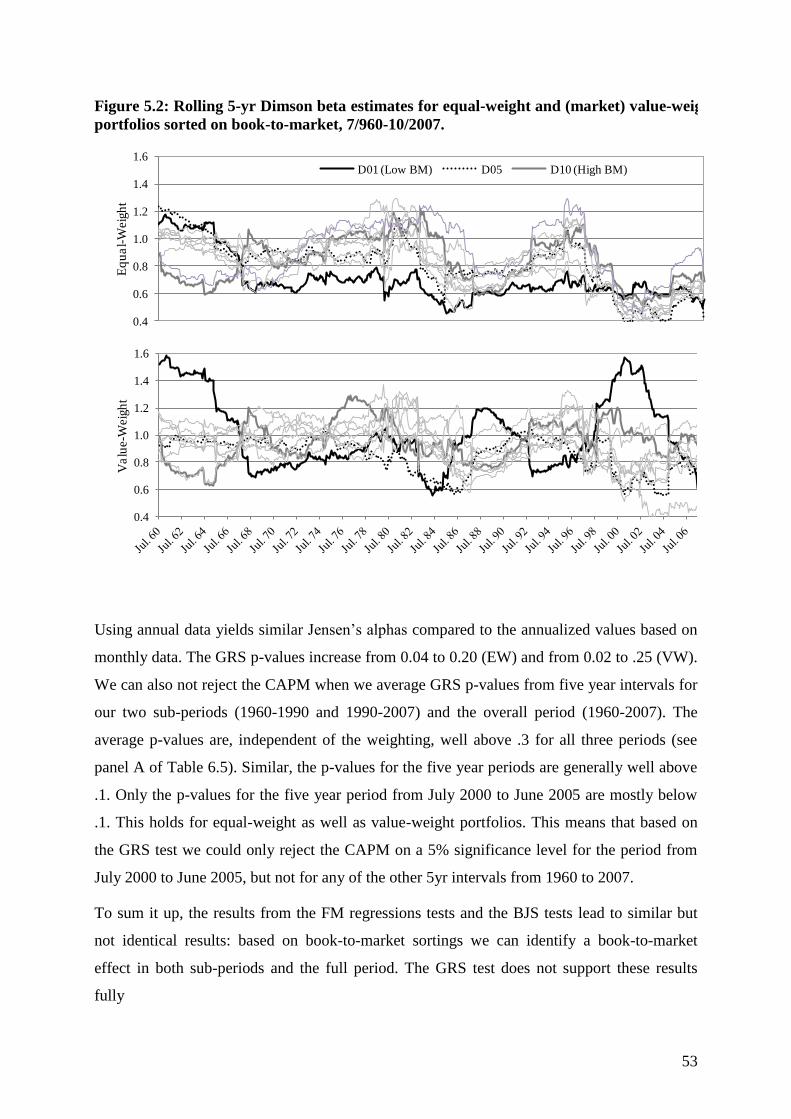
53
Using annual data yields similar Jensen’s alphas compared to the annualized values based on
monthly data. The GRS p-values increase from 0.04 to 0.20 (EW) and from 0.02 to .25 (VW).
We can also not reject the CAPM when we average GRS p-values from five year intervals for
our two sub-periods (1960-1990 and 1990-2007) and the overall period (1960-2007). The
average p-values are, independent of the weighting, well above .3 for all three periods (see
panel A of Table 6.5). Similar, the p-values for the five year periods are generally well above
.1. Only the p-values for the five year period from July 2000 to June 2005 are mostly below
.1. This holds for equal-weight as well as value-weight portfolios. This means that based on
the GRS test we could only reject the CAPM on a 5% significance level for the period from
July 2000 to June 2005, but not for any of the other 5yr intervals from 1960 to 2007.
To sum it up, the results from the FM regressions tests and the BJS tests lead to similar but
not identical results: based on book-to-market sortings we can identify a book-to-market
effect in both sub-periods and the full period. The GRS test does not support these results
fully
Figure 5.2: Rolling 5-yr Dimson beta estimates for equal-weight and (market) value-weight
portfolios sorted on book-to-market, 7/960-10/2007.
0.4
0.6
0.8
1.0
1.2
1.4
1.6
Eq
ua
l-W
eig
ht
D01 (Low BM) D05 D10 (High BM)
0.4
0.6
0.8
1.0
1.2
1.4
1.6
Va
lue-W
eig
ht
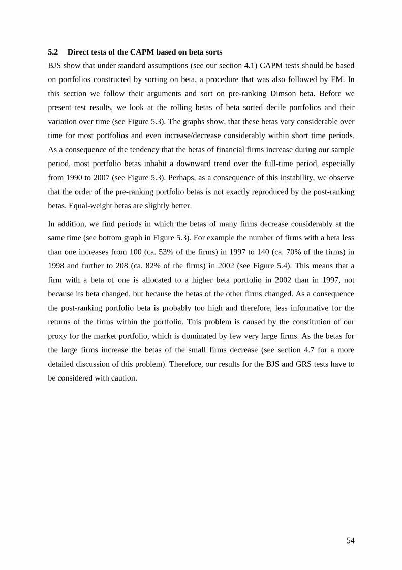
54
5.2 Direct tests of the CAPM based on beta sorts
BJS show that under standard assumptions (see our section 4.1) CAPM tests should be based
on portfolios constructed by sorting on beta, a procedure that was also followed by FM. In
this section we follow their arguments and sort on pre-ranking Dimson beta. Before we
present test results, we look at the rolling betas of beta sorted decile portfolios and their
variation over time (see Figure 5.3). The graphs show, that these betas vary considerable over
time for most portfolios and even increase/decrease considerably within short time periods.
As a consequence of the tendency that the betas of financial firms increase during our sample
period, most portfolio betas inhabit a downward trend over the full-time period, especially
from 1990 to 2007 (see Figure 5.3). Perhaps, as a consequence of this instability, we observe
that the order of the pre-ranking portfolio betas is not exactly reproduced by the post-ranking
betas. Equal-weight betas are slightly better.
In addition, we find periods in which the betas of many firms decrease considerably at the
same time (see bottom graph in Figure 5.3). For example the number of firms with a beta less
than one increases from 100 (ca. 53% of the firms) in 1997 to 140 (ca. 70% of the firms) in
1998 and further to 208 (ca. 82% of the firms) in 2002 (see Figure 5.4). This means that a
firm with a beta of one is allocated to a higher beta portfolio in 2002 than in 1997, not
because its beta changed, but because the betas of the other firms changed. As a consequence
the post-ranking portfolio beta is probably too high and therefore, less informative for the
returns of the firms within the portfolio. This problem is caused by the constitution of our
proxy for the market portfolio, which is dominated by few very large firms. As the betas for
the large firms increase the betas of the small firms decrease (see section 4.7 for a more
detailed discussion of this problem). Therefore, our results for the BJS and GRS tests have to
be considered with caution.
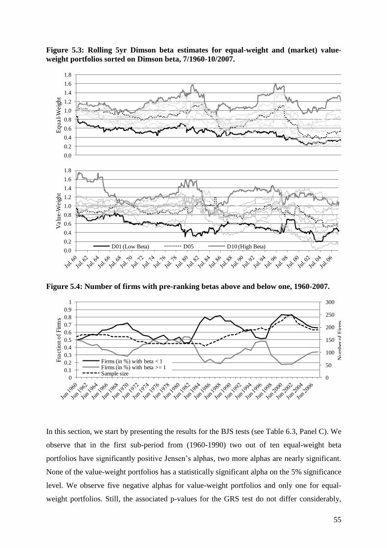
55
In this section, we start by presenting the results for the BJS tests (see Table 6.3, Panel C). We
observe that in the first sub-period from (1960-1990) two out of ten equal-weight beta
portfolios have significantly positive Jensen’s alphas, two more alphas are nearly significant.
None of the value-weight portfolios has a statistically significant alpha on the 5% significance
level. We observe five negative alphas for value-weight portfolios and only one for equal-
weight portfolios. Still, the associated p-values for the GRS test do not differ considerably,
Figure 5.3: Rolling 5yr Dimson beta estimates for equal-weight and (market) value-
weight portfolios sorted on Dimson beta, 7/1960-10/2007.
0.0
0.2
0.4
0.6
0.8
1.0
1.2
1.4
1.6
1.8
Eq
ua
l-W
eig
ht
0.0
0.2
0.4
0.6
0.8
1.0
1.2
1.4
1.6
1.8
Va
lue-W
eig
ht
D01 (Low Beta) D05 D10 (High Beta)
Figure 5.4: Number of firms with pre-ranking betas above and below one, 1960-2007.
0
50
100
150
200
250
300
0
0.1
0.2
0.3
0.4
0.5
0.6
0.7
0.8
0.9
1
Num
ber
of
Fir
ms
Fra
cti
on
of
Fir
ms
Firms (in %) with beta < 1 Firms (in %) with beta >= 1 Sample size

56
.28 (EW) vs. .30 (VW). In the second sub-period (1990-2007) the highest beta equal-weight
portfolio has an economically and statistically highly significant annualized alpha of -10.86%,
while the corresponding value-weight portfolio only has a Jensen’s alpha of -2.24% which is
not statistically significant. Furthermore, we observe negative alphas for the three equal-
weight portfolios with the highest betas. Only two of the corresponding value-weight
portfolios have negative alphas. In addition we find three positive and highly statistical
significant value-weight alphas, whilst none of the positive equal-weight alphas is significant.
These differences seem to be caused by the strong reverse size effect in this sub-period. The
GRS p-values are .03 (EW) and .04 (VW).
Comparing the alphas from both sub-periods with each other, we observe that the alphas of
the three highest beta equal-weight portfolios switch their signs from positive in the first to
negative in the second sub-period. This is not the case for the corresponding value-weight
portfolios. The sign of the alpha for the lowest beta portfolio changes for both weighting
schemes from negative to positive. The switch in signs of the alphas of the equal-weight
portfolios could also be attributed to the size effect. In the first sub-period, when we observe a
weak regular size-effect, small firms have positive alphas. In the second sub-period, when we
observe a strong reverse size effect, small firms have negative or lower alphas. As a
consequence the portfolio alphas vary over time.
When we look at the full time period (1960-2007) the seven equal-weight low beta portfolios
all have positive alphas, the three portfolios with a high beta all have negative alphas. These
results could indicate that the Black (1972) version of the CAPM holds in Germany. In
addition, three out of ten alphas are statistically significant different from zero on a 5%
significance level. The resulting GRS p-value of .04 rejects the CAPM at a 5% significance
level. The results for the corresponding value-weight portfolios are no cure to the CAPM. For
the full period the alphas are positive for most value-weight portfolios. They are negative for
the lowest beta portfolio and two of the three high beta portfolios. Three of the seven positive
alphas are statistically different from zero. This also translates into a GRS p-value of .04 for
the overall period.
In conclusion, we cannot reject the CAPM based on the GRS test for value-weight or equal-
weight beta sorted portfolios for the first sub-period from 1960 to 1990. For the second
period, however, the null that the CAPM holds is rejected on a 5% significance level. For the
full time period we would also reject the CAPM on a 5% significance level based on the GRS
test. Note that most of the underlying assumptions of the test procedure are violated. Portfolio

57
betas are not stationary. The BJS residuals are not normal i.i.d. As a consequence of the non-
normality of the residuals the power of the GRS test will be overstated and the p-values of the
GRS test statistic too low.
We continue by looking at the results of the FM tests. These provide further evidence in favor
of the CAPM. Again, we observe that in cross-sectional regressions weighting matters. We
would draw very different conclusions looking at average slopes on betas obtained from
equal-weight vs. value-weight portfolios. Equal-weight portfolios yield slopes which are
generally positive in the first sub-period, generally negative in the second sub-period (1990-
2007), and mostly negative in the overall period. The slopes on beta are, however, not
statistically significant. This observation does not change when we try to increase the spread
in post-ranking portfolio betas by forming 16 or 20 portfolios instead of ten. The results are
also stable with respect to the return interval (monthly, quarterly, annual returns), the
procedure to estimate post-ranking betas (full period, rolling) and whether we look at firm or
portfolio data.
For value-weight portfolios, we obtain, with some exceptions in the second sub-period,
positive slopes on beta in all periods. This result is robust to all the above mentioned
variations in the FM test procedure. However, the slopes are not statistically significant
different from zero. This issue causes some authors to conclude that the CAPM is dead.
Grauer/Janmaat (2009) conclude that such statements “may be greatly exaggerated”, because
cross-sectional “tests of whether the slope is equal to zero lack power”.119
Another result of
Grauer/Janmaat (2009) is that tests of a zero intercept are informative: For value-weight
portfolios rejection rates are down to 5% for 360 and more observations. For equal-weight
portfolios they show, that the rejection rates increase as the number of observation increases,
hence such test might incorrectly indicate that the CAPM should be rejected. The alphas for
our value-weight portfolios are not statistically different from zero for the full period. The
same applies to the first sub-period, most t-values are very close to zero. In the second sub-
period, however, the alphas are generally positive and statistically different from zero. When
we increase the number of portfolios from 10 to 16 and 20, the t-value on alpha decreases. For
twenty beta portfolios only few of the alphas from value-weight portfolios are statistically
significant. For equal-weight portfolios, however, a different picture emerges. The alphas are
generally positive in all periods. They are generally statistically significant different from zero
in the second and the overall period for 10, 16 and 20 portfolios. Taking all this together (the
119
They also indicate in their Table 4 that results differ with respect to equal-weight and value-weight portfolios.
Rejecting the null of a zero slope is less likely for equal-weight portfolios.

58
results and the empirical problems), we interpret our cross-sectional results as further
evidence in support of the CAPM.
The results for the slopes on betas are quite robust with respect to an omitted variable bias.
The slopes are generally positive in all periods and for most variations when we look at value-
weight portfolios. For equal-weight portfolios the slopes are positive in the first period only,
whereas, they are generally negative in the second sub-period and the full period. With
respect to alphas we observe that adding additional independent variables to the model
generally yields higher alphas in the first sub-period. For the second sub-period and the full
period alphas are generally lower. Including both variables, size and book-to-market, in the
model has the largest effect on the magnitude of the alphas.
In a model extended by size we observe positive slopes on beta for the first sub-period (most
statistically significant) and for the full period (some are statistically significant at the 10%
level) when we use value-weight portfolios. In the second sub-period the results for slopes on
beta are mixed. None are statistically significant different from zero. In all three periods we
find some negative alphas for the value-weight portfolios. They are, however, not statistically
significant in the two sub-periods nor in the full period. For equal-weight portfolios the slopes
on beta are also positive in the first sub-period (all alphas are positive and some statistically
significant) and the full period (some are negative, none are statistically significant). In the
second sub-period all alphas are negative, none statistically significant, though. In all three
periods we observe only positive alphas, some alphas are also statistically significant in the
full period.
In a model extended by book-to-market we also observe mostly positive, statistically
insignificant slopes for the first sub-period (always positive), the second sub-period (mixed)
and the full period (most positive) when we look at value-weight portfolios. The slopes are
not statistically significant. In all period alphas are positive, but generally not statistically
significant. Equal-weight portfolios yield negative slopes for the second sub-period and the
full period. Most slopes on beta in the first sub-period remain positive. None of the sloped is
statistically significant. The alphas for the equal-weight portfolios are positive in all periods,
many of them are statistically significant at the 1% level in the second sub-period and the full
period. Some are also statistically significant in the first sub-period.
Extending the model by both, size and book-to-market does not change the results for beta
(see Table 6.7). The slope on beta remains generally positive in all periods when we look at
value-weight portfolios. Some are statistically significant in the first and/or second sub-
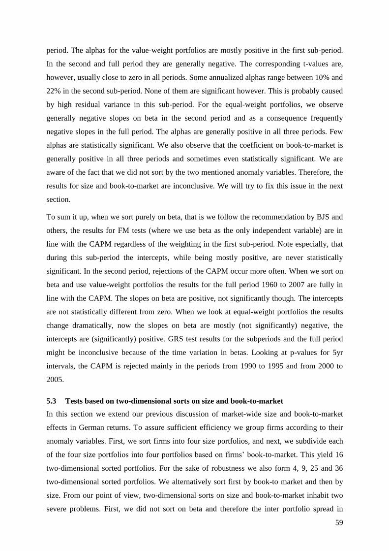
59
period. The alphas for the value-weight portfolios are mostly positive in the first sub-period.
In the second and full period they are generally negative. The corresponding t-values are,
however, usually close to zero in all periods. Some annualized alphas range between 10% and
22% in the second sub-period. None of them are significant however. This is probably caused
by high residual variance in this sub-period. For the equal-weight portfolios, we observe
generally negative slopes on beta in the second period and as a consequence frequently
negative slopes in the full period. The alphas are generally positive in all three periods. Few
alphas are statistically significant. We also observe that the coefficient on book-to-market is
generally positive in all three periods and sometimes even statistically significant. We are
aware of the fact that we did not sort by the two mentioned anomaly variables. Therefore, the
results for size and book-to-market are inconclusive. We will try to fix this issue in the next
section.
To sum it up, when we sort purely on beta, that is we follow the recommendation by BJS and
others, the results for FM tests (where we use beta as the only independent variable) are in
line with the CAPM regardless of the weighting in the first sub-period. Note especially, that
during this sub-period the intercepts, while being mostly positive, are never statistically
significant. In the second period, rejections of the CAPM occur more often. When we sort on
beta and use value-weight portfolios the results for the full period 1960 to 2007 are fully in
line with the CAPM. The slopes on beta are positive, not significantly though. The intercepts
are not statistically different from zero. When we look at equal-weight portfolios the results
change dramatically, now the slopes on beta are mostly (not significantly) negative, the
intercepts are (significantly) positive. GRS test results for the subperiods and the full period
might be inconclusive because of the time variation in betas. Looking at p-values for 5yr
intervals, the CAPM is rejected mainly in the periods from 1990 to 1995 and from 2000 to
2005.
5.3 Tests based on two-dimensional sorts on size and book-to-market
In this section we extend our previous discussion of market-wide size and book-to-market
effects in German returns. To assure sufficient efficiency we group firms according to their
anomaly variables. First, we sort firms into four size portfolios, and next, we subdivide each
of the four size portfolios into four portfolios based on firms’ book-to-market. This yield 16
two-dimensional sorted portfolios. For the sake of robustness we also form 4, 9, 25 and 36
two-dimensional sorted portfolios. We alternatively sort first by book-to market and then by
size. From our point of view, two-dimensional sorts on size and book-to-market inhabit two
severe problems. First, we did not sort on beta and therefore the inter portfolio spread in

60
portfolio betas, especially for value-weight portfolios, is rather small (see Table 6.2). For
value-weight portfolios the maximum spread in full-period betas over the full period is .54,
.51 for the first sub-period, and .69 for the second sub-period. As a consequence the efficiency
of the slope on beta in cross-sectional tests is low. In addition, according to Grauer/Janmaat
(2009) cross-sectional regressions also lack power to reject the null hypothesis that the slope
on betas is zero. Second, the procedures of BJS and FM (where we use a full-period beta)
assume stationary portfolio betas over time. Figure 5.5 indicates that this assumption is
violated for our value-weight double sorted size, book-to-market portfolios. Rolling beta
estimates for these portfolios vary considerably over time, most portfolio betas even exhibit a
remarkable downward trend.
We start by looking at the results for our FM regressions in Table 6.8 where we use beta, size
and book-to-market as independent variables. We address the problem of time varying betas
by additionally using rolling betas. There is a clear tendency for a regular market wide size
effect within the first sub-period. The sign of the coefficient on size is negative in all
variations of the FM test procedure (return interval, beta estimation, weighting, number of
portfolios). The effect is not statistically significant when we look at 4x4 sorts. An attempt to
increase the intra portfolio spread in size, by looking at 5x5 sorts yields mostly statistically
significant coefficients on size. When we further increase the spread in size, by looking at 6x6
sorts, yields coefficients on size that are again mostly not statistically significant. The
coefficient on size is also not statistically significant for firm level data. Nevertheless, our
results for the first sub-period support Stehle’s (1997) conclusion that a regular size effect
existed in Germany before 1990.
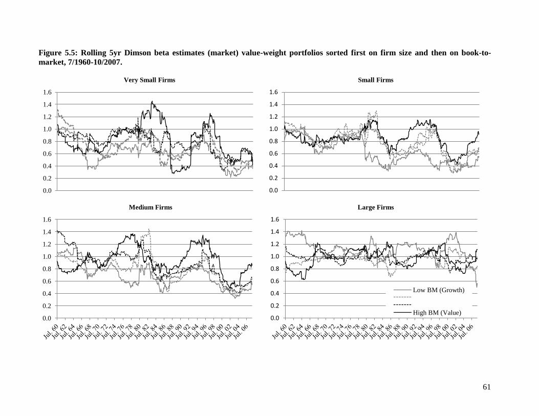
61
Figure 5.5: Rolling 5yr Dimson beta estimates (market) value-weight portfolios sorted first on firm size and then on book-to-
market, 7/1960-10/2007.
0.0
0.2
0.4
0.6
0.8
1.0
1.2
1.4
1.6
Very Small Firms
0.0
0.2
0.4
0.6
0.8
1.0
1.2
1.4
1.6
Small Firms
0.0
0.2
0.4
0.6
0.8
1.0
1.2
1.4
1.6
Medium Firms
0.0
0.2
0.4
0.6
0.8
1.0
1.2
1.4
1.6
Large Firms
Low BM (Growth)
High BM (Value)
62
We draw a completely different picture for the second sub-period, the slope on size is negative
and statistically significant for almost all variations in the test procedure. A strong reverse size
effect prevails. The annualized coefficient on size is on average almost 3% (with a range of 2% to
4%). The reverse size effect in the second sub-period is strong enough to manifest into the overall
period. For most variations in firm level regressions the reverse size effect is statistically
significant (or nearly) in the full period, even though it stems from the second sub-period only.
The results for the book-to-market variable are more stable across the two sub-periods. For all
variations of our test procedure the coefficients on book-to-market are positive and mostly
statistically significant. As a consequence of the stability of the book to market effect across both
sub-periods it is statistically significant for all variations of the test procedures in the full period.
However, some patterns with respect to book-to-market emerge. (1) The coefficients on book-to-
market and the t-values tend to be lower during the second period compared to the first period.
(2) They also tend to be lower for monthly returns compared to quarterly returns. (3) Looking at
value-weight returns also yields lower slopes on book-to-market and t-values compared to equal-
weight returns. For example, looking at value-weight portfolios yields slopes on book-to-market
during the second sub-period that are all not statistically significant on a 1% level, all t-values are
below 2.31. For equal-weight portfolios, however, the slopes are generally significant on a 1%
level during the same sub-period. (4) The coefficients of book-to-market are usually lowest when
we use rolling post-ranking betas instead of full period or annual betas in monthly FM
regressions. In the full period it is approximately 30 to 45% lower. The corresponding t-values
also decrease by approximately 30%. Monthly regression of value-weight portfolios sorted first
on size and then on book-to-market (4x4) where we include monthly rolling betas as an
independent variable yields quite favorable result for the CAPM. For these portfolios the t-values
on book-to-market are below 1.64 in the first and second sub-period, for the full period the t-
value is 1.99. The t-values for size are -1.71 in the first sub-period, 3.61 in the second and 1.14 in
the full period. Slopes on beta are positive in the first sub-period (t-value is 1.73) and the overall
period, but negative in the second sub-period, not significant, however. We generally obtain the
most unfavorable results for the CAPM when we look at results for firm level regressions.
Next we briefly look at the intercepts from our cross-sectional FM regressions. In the first sub-
period all intercepts are positive, most are statistically significant. The magnitude of the intercept
is considerably high, on average 7.90% (EW) and 7.3% (VW). For the second sub-period the
63
intercepts are all negative, on average -8.38% (EW) and -6.66% (VW). Most alphas are,
however, not statistically significant. In the full period most alphas are positive on average 2.52%
(EW) and 2.34% (VW), none is statistically significant. The t-values are close to zero, though.
These results are supported by a reduced model where only size and book-to-market enter as
independent variables.
Now, we continue with the BJS and GRS test results. Using monthly return data we observe a
strong book-to-market effect within the four portfolios in the top size ranking. The portfolio with
lowest book-to-market has a negative alpha, the portfolios with highest book-to-market has a
positive alpha. This effect exists in both sub-periods and as a consequence in the full period, it
exists regardless of which ranking criterion is used first and of the weighting. This effect also
persists in the group of portfolios with the second highest size ranking, somewhat less
pronounced, but also in both sub-periods, the full period and regardless of the ranking order and
weighting procedure. This effect also shows up in the four book-to-market portfolios that contain
the smallest firms, but only in the first sub-period (1960-1990). Among those portfolios the one
with highest book-to-market has an alpha which is economically and statistically highly
significant, regardless of the ranking criterion used first and of the weighting. In the second sub-
period (1990-2007) all four book-to-market portfolios of small firms have negative or neutral
alphas. The two portfolios of the firms with highest book-to-market have the most negative. This
‘reverse book-to-market effect’ among the smallest firms in the second sub-period shows up most
strongly, when we look at value-weight portfolios sorted first on the book-to-market ratio
(t=-3,22), but also in equal-weight portfolios. A regular book-to-market effect also exists in the
full period for the smallest firms, but as a consequence of the reverse book-to-market effect in the
second sub-period, it is less pronounced than for the three higher size groups.
The portfolio of small, high book-to-market firms has a positive, statistically significant alpha in
the first sub-period, and a negative, usually also significant in the second sub-period. As a
consequence, this portfolio has a near neutral risk-adjusted performance over all. Large, high
book-to-market firms have a positive alpha in the first sub-period and perform economically and
statistically even better in the second. As a consequence their risk-adjusted return is significantly
positive in the over-all period. Large, low book to market firms have an extremely poor risk-
adjusted return in the first sub-period, in the second sub-period the alpha is just slightly negative.
As a consequence their risk-adjusted return is usually significantly negative in the over-all period.
64
An important conclusion therefore is that the book-to-market effect in Germany varies over time
within the different size classes, for some portfolios considerably.
Loughran (1997) concludes that the book-to-market effect is “mostly a manifestation of the low
returns on small newly-listed growth stocks outside of January coupled with a seasonal January
effect for value firms.” Furthermore Loughran (1997) concludes that “[f]or the largest size
quintile (accounting for, on average, 73% of all market value), book-to-market has no reliable
predictive power for [U.S.] returns during the 1963-1995 period.”120
Fama/French (2008)
conclude for the period from 1963 to 2005 that the book-to-market effect is consistent across
different size groups. However, for the U.S. they also observe a stronger relation between
average returns and book-to-market for microcaps and small stocks compared to large stocks 121
We observe for the period from 1960 to 1990 a strong book-to-market effect among small and
large firms in both raw returns and risk-adjusted returns. However, for the second period the
book-to-market effect tends to vanish or even reverse for small firms. The effect also tends to
disappear for the firms from the large firm quartile when we first sort by size. The raw returns
and alphas of these firms are virtually flat (close to zero), except for the highest book-to-market
firms. The book-to-market effect is more pronounced during the second sub-period among large
firms when we sort by book-to-market first. Therefore, our results for a book-to-market effect
among large firms tends to be in line with the international evidence of Fama/French (2006).
Based on the analysis of Jensen’s alphas we are not able to clearly distinguish between the book-
to-market effect and the reverse size effect in the second sub-period. As mentioned above small
firms’ alphas are negative within the second sub-period across all book-to-market portfolios. This
result may probably be attributed to the fact that small firms performed poorly from 1990 to 2007
irrespective of their book-to-market. Large firms performed very well from 1990 to 2007,
especially those with higher book-to-market. Hence, the strong reverse size effect could
superpose the book-to-market effect, especially for the smallest firms and possibly amplify the
book-to-market effect for larger firms.
Now we briefly want to discuss the results from the GRS test. Looking at monthly returns for the
full period we would reject the CAPM on a 5% significance level for 4x4 sorts. Looking at
quarterly return data also yields p-values that reject the CAPM, even though they are usually
120
See Loughran (1997), p. 266-267. 121
See Fama/French (2008), p. 1667-1669.
65
higher. With annual return data, however, the p-values are sufficiently high to support the
CAPM. We generally estimate lower GRS p-values when we rank securities first by their book-
to-market and then by size. The results are also stable with respect to the number of portfolios.
However, the results for the GRS tests are dominated by the huge number of small stocks, which
enter the GRS test with a weight of approximately 50-75% depending on the number of
portfolios. Also be reminded that betas for these portfolios are not stable over time and that the
residuals from the BJS regression are not normal i.i.d. As a consequence we would assume higher
p-values, which would support the CAPM. We draw a completely different conclusion when we
look at average p-values for the same portfolios for non-overlapping 5yr intervals for the two
sub-periods and the overall period. Except for one incidence all p-values are well above .10 for
all variations in the test assets. We interpret these results as strong support for the CAPM. There
are, however, 5yr intervals where we obtain p-values below .10 for some variations in the test
assets. For the period from 7/2000 to 6/2005 all p-values are below (or very close to) .01.
Based on the FM results reported in Table 6.8, where all three variables are included, the BJS
results in Table 6.2, we conclude that there is a moderate market-wide regular size effect from
1960 to 1990. This effect reverses in the period from 1990 to 2007, where we observe an
economically and statistically significant reverse size effect. The book-to-market effect is more
stable over time, and mostly statistically significant in all three periods. Both effects are observed
in FM regressions at the same time, this means that size does not dominate book-to-market or
vice versa. Since we included beta as an independent variable, we have reason to assume that
these effects prevail in risk adjusted returns. These results are in line with the GRS test results in
Table 6.4.

66
6 Description of the data set
6.1 Sample selection
Empirical results generally vary to some extent with the sample constitution. Two questions
have to be carefully considered. First, which time period shall be covered? Second, which
assets should be included? Our initial data set includes all German firms where at least one
class of shares was listed in the top segment of the Frankfurt stock exchange, the Amtlicher
Markt, between December 1953 and October 2007.122
We restrict our data set to this period
for two reasons. First, book values of equity from 1948 to 1958 are currently not available to
us. Note however, we need a return series of 60 month to estimate pre-ranking firm betas to
group securities beginning at the end of June in 1958. Second, the Amtlicher Markt was
closed on October 31st, 2007. In order to avoid any selection bias, we include firms only for
the period for which they were actually listed in the Amtlicher Markt in Frankfurt. IPOs and
firms listed for the first time on an exchange are added to our data set at the end of the month
of their first listing in the Amtlicher Markt. We assume that our data set includes all German
firms for the entire time they are listed in the Amtlicher Markt in Frankfurt, and therefore, is
free of a survivorship bias.123
We include the common and preferred stocks of firms listed in the Amtlicher Markt in our
data set. Following the argument of previous studies we omit financial firms.124
We exclude
penny stocks, which we consider as stocks with share prices below €1 and an aggregated
market value over all share classes of less than €5 mln.125
We also remove profit participation
bonds (Genussscheine) from our dataset, which are also not considered in our estimates of the
122 Most studies for the German market as for example Oertmann (1994), Stehle (1997), Schlag/Wohlschließ
(1997), Wallmeier (2002), Schulz/Stehle (2002) Artmann/Finter/Kempf (2010) and
Artmann/Finter/Kempf/Koch/Theissen (2012) also include only stocks listed in Frankfurt. However, this
restriction is also a result of insufficient data availability and low data quality for other stock exchanges. In
section 2, we conclude that the Frankfurt stock exchange is representative for the German market. 123
Some studies for the German market as for example Artmann/Finter/Kempf/Koch/Theissen (2012) are not
free of a survivorship bias 124
See e.g., Fama/French (1992), p. 429; Fama/French (2008), p. 1677; Stehle (1994), p. 815; Schulz/Stehle
(2002), p. 13-14; Wright (2004), p. 561; Schrimpf/Schröder/Stehle (2007), p. 886; Artmann/Finter/Kempf
(2010), p. 4. 125
Our data suggests that most penny stocks are stocks of bankrupt or nearly bankrupt firms that no longer
publish financial statements.
67
book values of equity due to their debt character.126
Finally, we remove “Restquoten,”
bankrupt firms,127
and firms that are liquidated, but still exchange listed, from our data set.128
6.2 Book value of equity
We collected book values of equity from the Handbücher der Deutschen Aktiengesellschaft
(HBDA) for the period from 1957 to 1967. For the period from 1967 to 1990, we use the
same book values of equity as Schrimpf/Schröder/Stehle (2007). From 1990 we use the
Worldscope Financial Database (henceforth Worldscope) as the primary source for the book
values of equity.129
The data set of Schrimpf/Schröder/Stehle builds on data provided by the Deutsche
Finanzdatenbank (DFDB), and covers the years from 1967 to 2002.130
The data set from
HBDA and DFDB consist mainly of non-consolidated annual financial statements according
to the German accounting standard HGB. Book values of equity are adjusted for non-equity
components such as subscribed capital unpaid, treasury stocks and the equity portion of
special untaxed reserves.131
The book values from Worldscope consist mainly of consolidated
financial statements based on HGB (before 2005) and IFRS (after 2005). In cases in which
Worldscope did not report companies’ book values of equities we either use the data of
Schrimpf/Schröder/Stehle (2007), HBDA, or the Hoppenstedt Aktienführer.
We decided to switch from non-consolidated statements according to the German HGB to
consolidated statements, because according to Gehrke (1994) few firms published
consolidated annual financial statements including foreign subsidiaries before 1986.132
In
addition, the number of firms for which we have access to non-consolidated HGB statements
decreases rapidly after 2002. This means that consolidated statements are only applied before
December 1990 if non-consolidated statements are not available. We observe that the number
126 See Stehle (1994), S. 816.
127 E.g. the Bremer Bremer Vulkan Verbund AG filed for bankruptcy in May 1996, but was listed in the AM_F
until June 2006. 128
E.g. although, on May 26th
, 1966 the share holders of Riebeck’sche Montanwerke AG decided to liquidate
the company, its shares were listed in the AMF until September 9th
, 1982 and in the Freiverkehr (the lowest
market segment) in Frankfurt until 2002. For the same reason we removed Mauser Waldeck AG (liquidated
since October 22nd
, 2002) and I.G. Farbenindustrie AG (liquidated since February 1st, 1952) from our data
set. 129
WFD data type: WC03501. 130
See Schrimpf/Schröder/Stehle (2007), p. 886. 131
See Schulz/Stehle (2002), p. 10, and Stehle (1994), p. 817 for details on estimating the book value of equity. 132
See Gehrke (1994), p. 53-55. The Bilanzrichtlinien-Gesetz (BiRiLiG) from December 19th
, 1985
implemented the 7th
EG-Richtlinie, which specified that firms have to include foreign subsidiaries in their
consolidated statements for financial years starting on December 31st , 1989. See Küting/Weber (1987).

68
of firms for which Worldscope reports consolidated statements according to IFRS rapidly
increases after 2001, whereas the fraction of HGB statements steadily decreases.
6.3 Market value of equity (firm size)
We generally estimate the market value of equity (as a proxy for firm size) as the product of
the stock price and the number of shares outstanding as of the end of each month. The number
of shares outstanding was initially obtained by Stehle/Hartmond (1991) until the end of 1995
and by Schulz/Stehle (2002) for 1996 to 2002. We supplemented this data for the years 2003
to 2007 using Datastream (data type: NOSH). We carefully examined the quality of the data
on the number of shares for the whole period using the Hoppenstedt Aktienführer, Saling
Aktienführer and Handbuch der Deutschen Aktiengesellschaft. In addition, we cross-checked
and corrected the number of shares using our data on stock splits, stock dividends, right
issues, and reverse stock splits.
We identified 38 stocks for which the number of shares outstanding differs significantly from
the number of listed shares. The most prominent example of such a firm is the Deutsche
Telekom AG, which issued approximately 2.993 billion shares of which only 1 billion were
listed from November 1996 to May 1999. We believe that adjusting the market value of
equity for unlisted shares improves our firm size estimate.
Firm size is measured by the market value of the total equity of a firm. A firm’s equity
portfolio value is typically calculated on the basis of the common and preferred stock prices
and the number of shares issued in both classes.133
However, we identified 42 firms that had
for some time period only their preferred stocks listed in the Amtlicher Markt, but not their
common stocks. If only one type of stocks is exchange listed, we use its price to estimate the
market value of the unlisted type.134
We also identified 3 cases where only the common stocks
but not the preferred stocks were listed.
We calculate the book-to-market ratio using the aforementioned aggregated market
capitalization over all listed and unlisted share classes. We apply the same market value of
equity as a proxy for firm size. However, we take the market value of listed shares only (the
133 We adjust our proxy for firm size for the market value of share classes that were not listed in the AMF, but in
another market segment or at another stock exchange. E.g.: Glunz AG and König&Bauer AG. 134
Daske/Erhardt show that between 1956 and 1998 the prices of common stocks in the AMF are on average
19.18% higher than the prices of the preferred stocks. However, due to the fact that this difference is not
stable over time we refuse to adjust the common stocks’ prices. See Daske/Erhardt (2002), p. 20-21. The
data for the non-listed common stocks was kindly provided by Stefan Daske.

69
aggregate over all share classes) when we calculate market-value weighted rates of return of
portfolios. We use the natural logarithm of firm size and the B/M-ratio as independent
variables in our cross-sectional regressions.
6.4 Rates of return calculation
The data required to calculate stocks’ monthly rates of return is obtained from a database for
the Amtlicher Markt, which covers the period from 1953 to October 2007. This database was
initially established and described by Stehle/Hartmond (1991). The original database was
supplemented by Schulz/Stehle (2002) and Brückner/Stehle (2011) until October 2007.135
The
data was primarily obtained from the Hoppenstedt Kurstabellen, the Hoppenstedt
Aktienführer, Saling Aktienführer, Handbuch der Deutschen Aktiengesellschaft, the
Karlsruher capital market database (KMDB),136
Thomson Datastream, and the Börsenzeitung.
The database generally contains the following data types: i) the last price of each month, ii)
the number of shares outstanding, iii) dividends and information on pure stock splits, iv) stock
dividends, v) right issues, vi) reverse stock splits, and vii) other financial benefits. We
estimate the rates of return of firms that have multiple share classes outstanding as the value-
weighted rate of return over all listed share classes in the Amtlicher Markt.
We calculate monthly rates of return from the perspective of small domestic investors. This
means that we adjust the monthly rates of return for share reallocations from majority to
minority share holders,137
dividends which are only distributed to minority or free share
holders138
and corporate income tax credits (Körperschaftsteuergutschrift). For firms with
multiple share classes we aggregate the rates of return by the exchange listed market
capitalization of each share class. This means that we are creating artificial assets, which are
considered in our empirical tests.
6.5 Estimating portfolio characteristics
We generally form our characteristic portfolios as of the end of June of year t. Portfolios’
equal-weighted and value-weighted monthly, quarterly and annual returns are estimated for
the period from July in year t to June in year t+1, from t = 1958 to 2007. Based on these
135 The data set was applied among others by Schrimpf/Schröder/Stehle (2007), Ziegler/Schröder/Schulz/Stehle
(2007), Brückner/Stehle (2010), and Pryshchepa/Stehle (2010). 136
See Bühler/Göppl/Möller (1993), p. 291-303; Herrmann (1996). 137
E.g. in November 1993 FAG Kugelfischer AG, the majority share holder of Dürkopp Adler AG, distributed
one for ten shares of Dürkopp Adler AG to all minority share holders of that company. 138
E. g. Audi AG and MAN Roland Druckmaschinen AG.

70
portfolio returns we estimate portfolios’ post-ranking full-period and rolling betas, regressing
the returns of the portfolio on our value-weighted proxy for the market portfolio. Dimson
betas include the one-period lagged market return. Rolling betas are estimated based on a 24
to 60 month period (as available).
Portfolio size ,P tSize and book-to-market
,P tBM are estimated following
Kothari/Shanken/Sloan (1995) as:
,
, , ,
1
lnP tN
P t i t i t
i
Size w Size
, and
,
, , ,
1
lnP tN
P t i t i t
i
BM w BM
(1)
where ,P tN is the number of firms in portfolio P as of June in year t, ,i tw is the weight of firm
i as of June in year t in portfolio P, ,i tSize is the market value of equity of firm i as of June in
year t, and ,i tBM is book-to-market of firm i as of June in year t (estimated as of December in
year t-1). We estimate ,i tw as 1
, ,i t P tw N for equal-weighted and as ,
, , ,
1
P tN
i t i t j t
j
w Size Size
for
value-weighted portfolios.
Note, it would also be reasonable to estimate portfolios’ size and book-to-market averaging
the natural logarithms of firms’ characteristics. Hence we could alternatively use:
,
, , ,
1
lnP tN
P t i t i t
i
Size w Size
and ,
, , ,
1
lnP tN
P t i t i t
i
BM w BM
(2)
We decided to estimate portfolios size and book-to-market characteristics according to
equation (1), since we believe that it is more in line with the literature. However, the
difference between both measures (equation 1 vs. 2) depends on the intra-portfolio spread in
firms’ size. Hence, we assume that this issue is relevant only in cross-sectional regressions
that include portfolio size as an independent variable when portfolios are not formed on size.
For size sorted portfolios, the difference should be negligible.

71
6.2 Tables and Figures
All our portfolios (test assets) and therefore all our results presented in the tables in this
appendix are based on exactly the same data set. Our grouping procedures only consider firms
with positive book-to-market and a return time series of at least 24 month as of the end of
June in year t. Financial firms and penny stocks are not considered by the grouping procedure.
In addition, we generally exclude the smallest 10% of the firms in our sample. Therefore, we
do not include the firms that have been assigned to size decile D01 (smallest firms in Table
6.1), (1) when we form 16 and 20 size portfolios, (2) when we sort by criterions other then
size, and (3) when we form two-dimensional groups.
Size is measured by a firms’ aggregate market value of equity over all share classes as of the
end of June in year t, also taking unlisted shares into account. Book-to-market is measured as
of the end of December in year t-1. Firms’ pre-ranking Dimson Betas are estimated at the end
of June in year t using a time series of 24 to 60 months (as available). We use these firm
characteristics to form our portfolios. Each portfolio represents approximately 1/k percent of
the firms, where k denotes the number of groups. The portfolios representing the firms with
the smallest characteristic usually include slightly more than 1/k percent of the firms. This is
due to the fact that we assign left over firms to these portfolios. For these portfolios we
calculate monthly, quarterly, and annual rates of returns from July in year t to June in year
t+1.
We present portfolio characteristics and regression results for the overall period from July
1960 to October 2007 as well as two sub-periods. The first sub-period extends from July 1960
to June 1990, the second from July 1990 to June 2007. We also present results for equal-
weight as well as value-weight portfolios.
Table 6.1: Descriptive statistics and empirical results for one-dimensional sorts (decile
portfolios) on size, book-to-market and Dimson beta, 07/1960-06/1990, 07/1990-10/2007,
and 07/1960-10/2007.
The following three panels, A, B, and C of this table present descriptive statistics for one-dimensional sorted
decile portfolios. Portfolios are formed by sorts on size (panel A), book-to-market (panel B), and Dimson beta
(panel C). Portfolios’ average monthly excess rate of return is estimated as the arithmetic mean of the portfolios’
return less the risk-free rate (SU0104). We estimate the monthly standard deviations of the rates of return from
annual rates of return. Pre-ranking Dimson betas are the averages of a portfolio’s firms pre-ranking Dimson
betas as of the end of June in year t. Post-ranking Dimson betas are estimated using the full return time series for
the stated period. Jensen’s alphas are the intercepts from equation (1) in section 4.1; a time series regression á la
BJS extended by the lagged market excess rate of return to adjust for the infrequent trading bias. The differences
between the results from the standard and the extended BJS model are marginal. We annualize monthly alphas
multiplying them with 12. The t-values for the alphas are Newey/West (1994) adjusted. We also present GRS test
statistics and the associated p-values based on monthly return intervals. The bottom rows present the average,
inflation adjusted size of a portfolio.
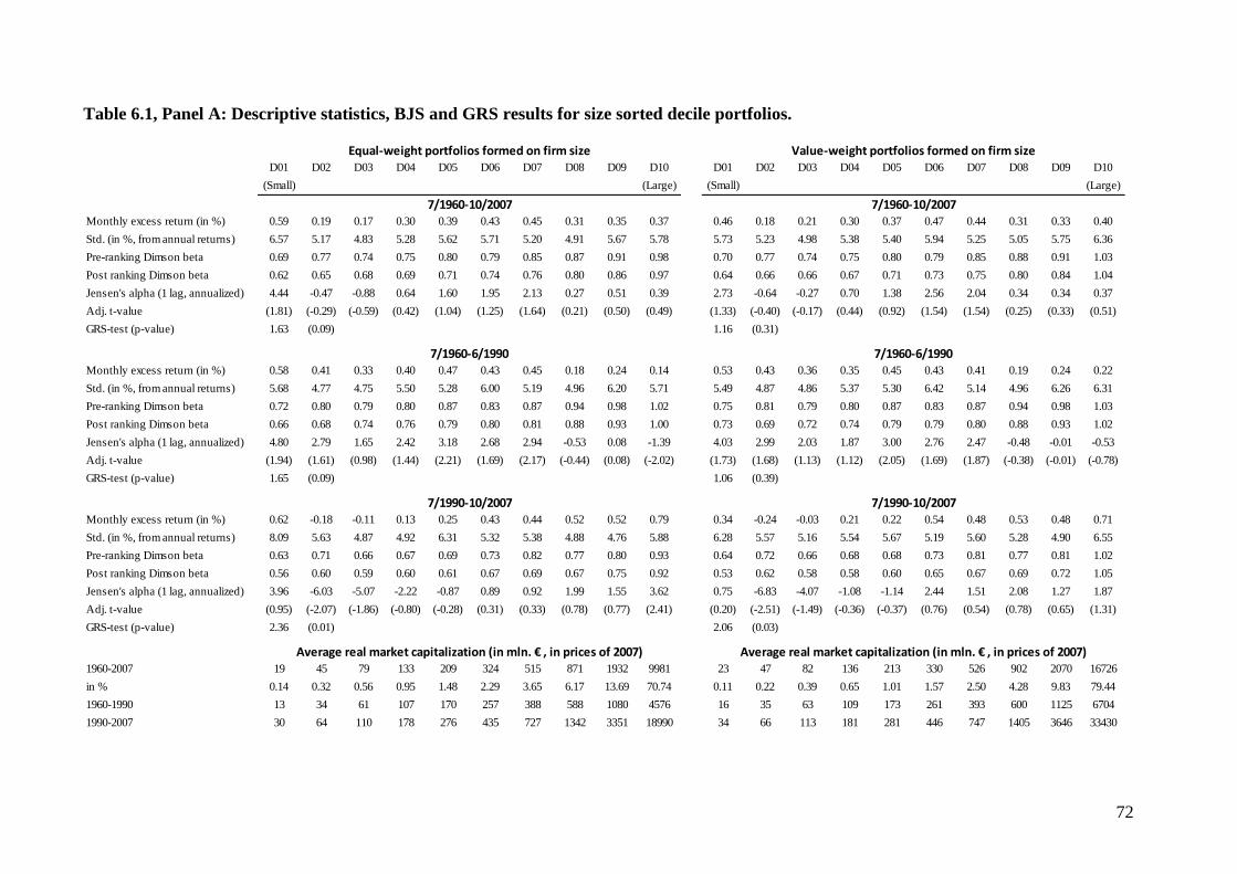
72
Table 6.1, Panel A: Descriptive statistics, BJS and GRS results for size sorted decile portfolios.
D01 D02 D03 D04 D05 D06 D07 D08 D09 D10 D01 D02 D03 D04 D05 D06 D07 D08 D09 D10
(Small) (Large) (Small) (Large)
Monthly excess return (in %) 0.59 0.19 0.17 0.30 0.39 0.43 0.45 0.31 0.35 0.37 0.46 0.18 0.21 0.30 0.37 0.47 0.44 0.31 0.33 0.40
Std. (in %, from annual returns) 6.57 5.17 4.83 5.28 5.62 5.71 5.20 4.91 5.67 5.78 5.73 5.23 4.98 5.38 5.40 5.94 5.25 5.05 5.75 6.36
Pre-ranking Dimson beta 0.69 0.77 0.74 0.75 0.80 0.79 0.85 0.87 0.91 0.98 0.70 0.77 0.74 0.75 0.80 0.79 0.85 0.88 0.91 1.03
Post ranking Dimson beta 0.62 0.65 0.68 0.69 0.71 0.74 0.76 0.80 0.86 0.97 0.64 0.66 0.66 0.67 0.71 0.73 0.75 0.80 0.84 1.04
Jensen's alpha (1 lag, annualized) 4.44 -0.47 -0.88 0.64 1.60 1.95 2.13 0.27 0.51 0.39 2.73 -0.64 -0.27 0.70 1.38 2.56 2.04 0.34 0.34 0.37
Adj. t-value (1.81) (-0.29) (-0.59) (0.42) (1.04) (1.25) (1.64) (0.21) (0.50) (0.49) (1.33) (-0.40) (-0.17) (0.44) (0.92) (1.54) (1.54) (0.25) (0.33) (0.51)
GRS-test (p-value) 1.63 (0.09) 1.16 (0.31)
Monthly excess return (in %) 0.58 0.41 0.33 0.40 0.47 0.43 0.45 0.18 0.24 0.14 0.53 0.43 0.36 0.35 0.45 0.43 0.41 0.19 0.24 0.22
Std. (in %, from annual returns) 5.68 4.77 4.75 5.50 5.28 6.00 5.19 4.96 6.20 5.71 5.49 4.87 4.86 5.37 5.30 6.42 5.14 4.96 6.26 6.31
Pre-ranking Dimson beta 0.72 0.80 0.79 0.80 0.87 0.83 0.87 0.94 0.98 1.02 0.75 0.81 0.79 0.80 0.87 0.83 0.87 0.94 0.98 1.03
Post ranking Dimson beta 0.66 0.68 0.74 0.76 0.79 0.80 0.81 0.88 0.93 1.00 0.73 0.69 0.72 0.74 0.79 0.79 0.80 0.88 0.93 1.02
Jensen's alpha (1 lag, annualized) 4.80 2.79 1.65 2.42 3.18 2.68 2.94 -0.53 0.08 -1.39 4.03 2.99 2.03 1.87 3.00 2.76 2.47 -0.48 -0.01 -0.53
Adj. t-value (1.94) (1.61) (0.98) (1.44) (2.21) (1.69) (2.17) (-0.44) (0.08) (-2.02) (1.73) (1.68) (1.13) (1.12) (2.05) (1.69) (1.87) (-0.38) (-0.01) (-0.78)
GRS-test (p-value) 1.65 (0.09) 1.06 (0.39)
Monthly excess return (in %) 0.62 -0.18 -0.11 0.13 0.25 0.43 0.44 0.52 0.52 0.79 0.34 -0.24 -0.03 0.21 0.22 0.54 0.48 0.53 0.48 0.71
Std. (in %, from annual returns) 8.09 5.63 4.87 4.92 6.31 5.32 5.38 4.88 4.76 5.88 6.28 5.57 5.16 5.54 5.67 5.19 5.60 5.28 4.90 6.55
Pre-ranking Dimson beta 0.63 0.71 0.66 0.67 0.69 0.73 0.82 0.77 0.80 0.93 0.64 0.72 0.66 0.68 0.68 0.73 0.81 0.77 0.81 1.02
Post ranking Dimson beta 0.56 0.60 0.59 0.60 0.61 0.67 0.69 0.67 0.75 0.92 0.53 0.62 0.58 0.58 0.60 0.65 0.67 0.69 0.72 1.05
Jensen's alpha (1 lag, annualized) 3.96 -6.03 -5.07 -2.22 -0.87 0.89 0.92 1.99 1.55 3.62 0.75 -6.83 -4.07 -1.08 -1.14 2.44 1.51 2.08 1.27 1.87
Adj. t-value (0.95) (-2.07) (-1.86) (-0.80) (-0.28) (0.31) (0.33) (0.78) (0.77) (2.41) (0.20) (-2.51) (-1.49) (-0.36) (-0.37) (0.76) (0.54) (0.78) (0.65) (1.31)
GRS-test (p-value) 2.36 (0.01) 2.06 (0.03)
1960-2007 19 45 79 133 209 324 515 871 1932 9981 23 47 82 136 213 330 526 902 2070 16726
in % 0.14 0.32 0.56 0.95 1.48 2.29 3.65 6.17 13.69 70.74 0.11 0.22 0.39 0.65 1.01 1.57 2.50 4.28 9.83 79.44
1960-1990 13 34 61 107 170 257 388 588 1080 4576 16 35 63 109 173 261 393 600 1125 6704
1990-2007 30 64 110 178 276 435 727 1342 3351 18990 34 66 113 181 281 446 747 1405 3646 33430
Equal-weight portfolios formed on firm size Value-weight portfolios formed on firm size
Average real market capitalization (in mln. € , in prices of 2007)Average real market capitalization (in mln. € , in prices of 2007)
7/1960-10/2007
7/1960-6/1990
7/1990-10/2007
7/1960-10/2007
7/1960-6/1990
7/1990-10/2007

73
Table 6.1, Panel B: Descriptive statistics, BJS and GRS results for book-to-market sorted decile portfolios.
D01 D02 D03 D04 D05 D06 D07 D08 D09 D10 D01 D02 D03 D04 D05 D06 D07 D08 D09 D10
(Low) (High) (Low) (High)
Monthly excess return (in %) 0.03 0.28 0.20 0.28 0.29 0.35 0.33 0.48 0.44 0.69 0.04 0.20 0.35 0.08 0.41 0.39 0.47 0.52 0.69 0.84
Std. (in %, from annual returns) 4.17 5.05 4.65 5.29 5.23 4.92 5.03 6.19 6.23 6.66 7.45 5.97 6.39 6.97 6.09 5.85 5.11 6.53 7.23 7.81
Pre-ranking Dimson beta 0.73 0.76 0.81 0.85 0.82 0.90 0.91 0.90 0.86 0.81 0.93 0.88 0.93 1.05 0.91 0.94 0.97 0.96 0.95 0.90
Post-ranking Dimson beta 0.69 0.74 0.71 0.78 0.75 0.77 0.78 0.81 0.83 0.76 1.03 0.88 0.95 0.94 0.85 0.88 0.86 0.84 0.93 0.93
Jensen's Alpha (1 lag, annualized) -2.57 0.15 -0.60 -0.01 0.30 0.94 0.64 2.34 1.71 5.03 -3.94 -1.38 0.13 -3.08 1.32 0.89 1.92 2.60 4.37 6.15
Adj. t-Value (-2.07) (0.11) (-0.51) (-0.01) (0.23) (0.84) (0.43) (1.38) (0.98) (2.65) (-2.43) (-0.78) (0.09) (-1.99) (1.01) (0.71) (1.31) (1.39) (2.44) (3.23)
GRS-Test (p-Value) 1.90 0.04 2.10 (0.02)
Monthly excess return (in %) 0.07 0.27 0.19 0.18 0.33 0.31 0.35 0.40 0.53 0.87 -0.05 0.06 0.18 0.12 0.27 0.18 0.32 0.23 0.49 0.66
Std. (in %, from annual returns) 4.38 5.29 4.76 5.36 5.56 5.10 5.09 5.63 6.18 6.76 6.17 6.17 6.53 6.97 6.68 5.64 5.40 6.25 6.94 7.03
Pre-ranking Dimson beta 0.74 0.82 0.86 0.90 0.91 0.95 0.99 0.95 0.88 0.84 0.99 0.96 1.00 1.05 0.95 0.96 1.01 0.93 0.91 0.89
Post-ranking Dimson beta 0.72 0.81 0.76 0.86 0.84 0.86 0.86 0.89 0.86 0.78 0.59 0.63 0.83 0.88 0.87 0.90 0.93 0.95 1.06 1.27
Jensen's Alpha (1 lag, annualized) -1.41 0.68 -0.05 -0.52 1.39 1.11 1.52 2.01 3.67 7.95 -3.75 -2.11 -0.75 -1.67 0.52 -0.73 1.16 0.07 3.09 5.27
Adj. t-Value (-0.91) (0.44) (-0.04) (-0.41) (1.06) (1.01) (1.10) (1.46) (2.17) (3.82) (-2.35) (-1.20) (-0.47) (-1.00) (0.41) (-0.56) (0.84) (0.04) (1.57) (2.50)
GRS-Test (p-Value) 2.17 0.02 1.29 (0.23)
Monthly excess return (in %) -0.03 0.29 0.22 0.45 0.22 0.42 0.31 0.64 0.29 0.39 0.19 0.43 0.63 0.01 0.65 0.75 0.72 1.00 1.05 1.16
Std. (in %, from annual returns) 3.87 4.75 4.59 5.28 4.72 4.76 5.05 7.21 6.43 6.46 9.50 5.76 6.30 7.17 5.04 6.20 4.66 6.94 7.84 9.14
Pre-ranking Dimson beta 0.71 0.65 0.73 0.76 0.68 0.83 0.78 0.83 0.82 0.76 0.83 0.74 0.82 1.04 0.84 0.89 0.91 1.00 1.01 0.90
Post-ranking Dimson beta 0.65 0.64 0.64 0.66 0.63 0.64 0.68 0.71 0.81 0.75 1.05 0.80 0.94 0.85 0.79 0.81 0.86 0.77 0.97 1.02
Jensen's Alpha (1 lag, annualized) -4.46 -0.51 -1.37 1.18 -1.28 0.99 -0.61 3.20 -1.61 0.01 -4.33 0.09 1.68 -5.31 2.89 3.91 3.24 7.21 6.51 7.48
Adj. t-Value (-2.40) (-0.24) (-0.64) (0.45) (-0.47) (0.43) (-0.21) (0.83) (-0.48) (0.00) (-1.26) (0.02) (0.54) (-1.71) (1.08) (1.58) (1.02) (1.85) (1.91) (1.97)
GRS-Test (p-Value) 0.99 0.45 1.72 0.08
1960-2007 1827 1684 1569 2072 1749 1556 1609 1574 1089 872 11830 7249 8894 12570 9110 8116 8986 9919 5465 5138
in % 11.71 10.79 10.06 13.28 11.21 9.97 10.32 10.09 6.98 5.59 13.55 8.31 10.19 14.40 10.44 9.30 10.30 11.37 6.26 5.89
1960-1990 794 722 795 817 870 926 905 962 761 520 4459 3157 3285 3638 3248 4258 3488 3164 2301 1417
1990-2007 3550 3286 2860 4164 3215 2607 2784 2594 1636 1459 24115 14070 18242 27456 18880 14546 18149 21177 10737 11339
Equal-weight portfolios formed on B/M Value-weight portfolios formed on B/M
Average real market capitalization (in mln. € , in prices of 2007)
7/1960-10/20077/1960-10/2007
7/1960-6/1990 7/1960-6/1990
7/1990-10/2007 7/1990-10/2007
Average real market capitalization (in mln. € , in prices of 2007)
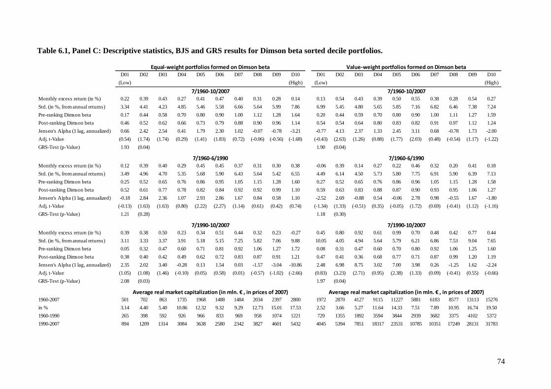
74
Table 6.1, Panel C: Descriptive statistics, BJS and GRS results for Dimson beta sorted decile portfolios.
D01 D02 D03 D04 D05 D06 D07 D08 D09 D10 D01 D02 D03 D04 D05 D06 D07 D08 D09 D10
(Low) (High) (Low) (High)
Monthly excess return (in %) 0.22 0.39 0.43 0.27 0.41 0.47 0.40 0.31 0.28 0.14 0.13 0.54 0.43 0.39 0.50 0.55 0.38 0.28 0.54 0.27
Std. (in %, from annual returns) 3.34 4.41 4.23 4.85 5.46 5.58 6.66 5.64 5.99 7.86 6.99 5.45 4.80 5.65 5.85 7.16 6.82 6.46 7.38 7.24
Pre-ranking Dimson beta 0.17 0.44 0.58 0.70 0.80 0.90 1.00 1.12 1.28 1.64 0.20 0.44 0.59 0.70 0.80 0.90 1.00 1.11 1.27 1.59
Post-ranking Dimson beta 0.46 0.52 0.62 0.66 0.73 0.79 0.88 0.90 0.96 1.14 0.54 0.54 0.64 0.80 0.83 0.82 0.91 0.97 1.12 1.24
Jensen's Alpha (1 lag, annualized) 0.66 2.42 2.54 0.41 1.79 2.30 1.02 -0.07 -0.78 -3.21 -0.77 4.13 2.37 1.33 2.45 3.11 0.68 -0.78 1.73 -2.00
Adj. t-Value (0.54) (1.74) (1.74) (0.29) (1.41) (1.83) (0.72) (-0.06) (-0.56) (-1.68) (-0.43) (2.63) (1.26) (0.88) (1.77) (2.03) (0.48) (-0.54) (1.17) (-1.22)
GRS-Test (p-Value) 1.93 (0.04) 1.90 (0.04)
Monthly excess return (in %) 0.12 0.39 0.40 0.29 0.45 0.45 0.37 0.31 0.30 0.38 -0.06 0.39 0.14 0.27 0.22 0.46 0.32 0.20 0.41 0.18
Std. (in %, from annual returns) 3.49 4.96 4.70 5.35 5.68 5.90 6.43 5.64 5.42 6.55 4.49 6.14 4.50 5.73 5.80 7.75 6.91 5.90 6.39 7.13
Pre-ranking Dimson beta 0.25 0.52 0.65 0.76 0.86 0.95 1.05 1.15 1.28 1.60 0.27 0.52 0.65 0.76 0.86 0.96 1.05 1.15 1.28 1.58
Post-ranking Dimson beta 0.52 0.61 0.77 0.78 0.82 0.84 0.92 0.92 0.99 1.10 0.59 0.63 0.83 0.88 0.87 0.90 0.93 0.95 1.06 1.27
Jensen's Alpha (1 lag, annualized) -0.18 2.84 2.36 1.07 2.93 2.86 1.67 0.84 0.58 1.10 -2.52 2.69 -0.88 0.54 -0.06 2.78 0.98 -0.55 1.67 -1.80
Adj. t-Value (-0.13) (1.63) (1.63) (0.80) (2.22) (2.27) (1.14) (0.61) (0.42) (0.74) (-1.34) (1.33) (-0.51) (0.35) (-0.05) (1.72) (0.69) (-0.41) (1.12) (-1.16)
GRS-Test (p-Value) 1.21 (0.28) 1.18 (0.30)
Monthly excess return (in %) 0.39 0.38 0.50 0.23 0.34 0.51 0.44 0.32 0.23 -0.27 0.45 0.80 0.92 0.61 0.99 0.70 0.48 0.42 0.77 0.44
Std. (in %, from annual returns) 3.11 3.33 3.37 3.91 5.18 5.15 7.25 5.82 7.06 9.88 10.05 4.05 4.94 5.64 5.79 6.21 6.86 7.53 9.04 7.65
Pre-ranking Dimson beta 0.05 0.32 0.47 0.60 0.71 0.81 0.92 1.06 1.27 1.72 0.08 0.31 0.47 0.60 0.70 0.80 0.92 1.06 1.25 1.60
Post-ranking Dimson beta 0.38 0.40 0.42 0.49 0.62 0.72 0.83 0.87 0.91 1.21 0.47 0.41 0.36 0.68 0.77 0.71 0.87 0.99 1.20 1.19
Jensen's Alpha (1 lag, annualized) 2.35 2.02 3.40 -0.28 0.13 1.54 0.03 -1.57 -3.04 -10.86 2.48 6.98 8.75 3.02 7.00 3.98 0.26 -1.25 1.62 -2.24
Adj. t-Value (1.05) (1.08) (1.46) (-0.10) (0.05) (0.58) (0.01) (-0.57) (-1.02) (-2.66) (0.83) (3.23) (2.71) (0.95) (2.38) (1.33) (0.09) (-0.41) (0.55) (-0.66)
GRS-Test (p-Value) 2.08 (0.03) 1.97 (0.04)
1960-2007 501 702 863 1735 1968 1488 1484 2034 2397 2800 1972 2870 4127 9115 11227 5881 6183 8577 13113 15276
in % 3.14 4.40 5.40 10.86 12.32 9.32 9.29 12.73 15.01 17.53 2.52 3.66 5.27 11.64 14.33 7.51 7.89 10.95 16.74 19.50
1960-1990 265 398 592 926 966 833 969 958 1074 1221 729 1355 1892 3594 3844 2939 3682 3375 4102 5372
1990-2007 894 1209 1314 3084 3638 2580 2342 3827 4601 5432 4045 5394 7851 18317 23531 10785 10351 17249 28131 31783
Average real market capitalization (in mln. € , in prices of 2007)
Value-weight portfolios formed on Dimson betaEqual-weight portfolios formed on Dimson beta
7/1960-10/2007
7/1960-6/1990
7/1990-10/2007
7/1960-6/1990
7/1990-10/2007
Average real market capitalization (in mln. € , in prices of 2007)
7/1960-10/2007
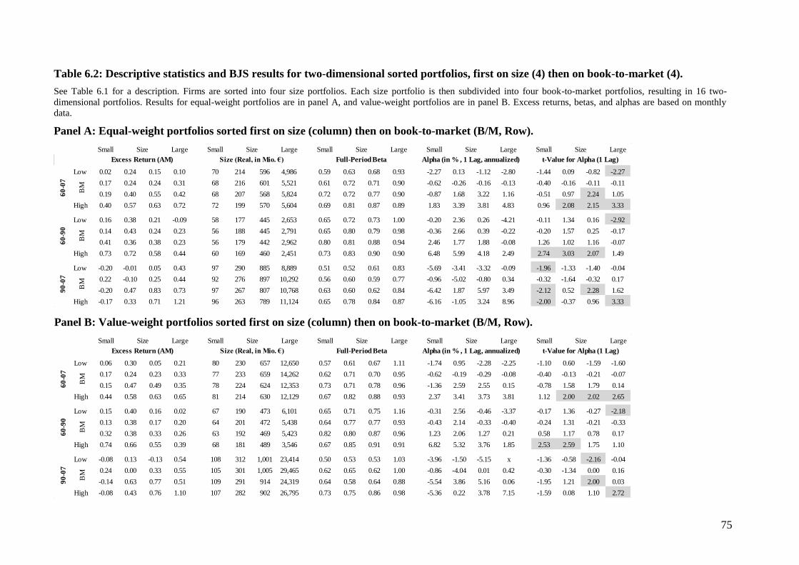
75
Panel B: Value-weight portfolios sorted first on size (column) then on book-to-market (B/M, Row).
Small Large Small Large Small Large Small Large Small Large
Low 0.06 0.30 0.05 0.21 80 230 657 12,650 0.57 0.61 0.67 1.11 -1.74 0.95 -2.28 -2.25 -1.10 0.60 -1.59 -1.60
0.17 0.24 0.23 0.33 77 233 659 14,262 0.62 0.71 0.70 0.95 -0.62 -0.19 -0.29 -0.08 -0.40 -0.13 -0.21 -0.07
0.15 0.47 0.49 0.35 78 224 624 12,353 0.73 0.71 0.78 0.96 -1.36 2.59 2.55 0.15 -0.78 1.58 1.79 0.14
High 0.44 0.58 0.63 0.65 81 214 630 12,129 0.67 0.82 0.88 0.93 2.37 3.41 3.73 3.81 1.12 2.00 2.02 2.65
Low 0.15 0.40 0.16 0.02 67 190 473 6,101 0.65 0.71 0.75 1.16 -0.31 2.56 -0.46 -3.37 -0.17 1.36 -0.27 -2.18
0.13 0.38 0.17 0.20 64 201 472 5,438 0.64 0.77 0.77 0.93 -0.43 2.14 -0.33 -0.40 -0.24 1.31 -0.21 -0.33
0.32 0.38 0.33 0.26 63 192 469 5,423 0.82 0.80 0.87 0.96 1.23 2.06 1.27 0.21 0.58 1.17 0.78 0.17
High 0.74 0.66 0.55 0.39 68 181 489 3,546 0.67 0.85 0.91 0.91 6.82 5.32 3.76 1.85 2.53 2.59 1.75 1.10
Low -0.08 0.13 -0.13 0.54 108 312 1,001 23,414 0.50 0.53 0.53 1.03 -3.96 -1.50 -5.15 x -1.36 -0.58 -2.16 -0.04
0.24 0.00 0.33 0.55 105 301 1,005 29,465 0.62 0.65 0.62 1.00 -0.86 -4.04 0.01 0.42 -0.30 -1.34 0.00 0.16
-0.14 0.63 0.77 0.51 109 291 914 24,319 0.64 0.58 0.64 0.88 -5.54 3.86 5.16 0.06 -1.95 1.21 2.00 0.03
High -0.08 0.43 0.76 1.10 107 282 902 26,795 0.73 0.75 0.86 0.98 -5.36 0.22 3.78 7.15 -1.59 0.08 1.10 2.72
60
-07
60
-90
90
-07
Size Size Size
Full-Period Beta t-Value for Alpha (1 Lag)Alpha (in % , 1 Lag, annualized)
Size
BM
BM
BM
Size
Excess Return (AM) Size (Real, in Mio. €)
Table 6.2: Descriptive statistics and BJS results for two-dimensional sorted portfolios, first on size (4) then on book-to-market (4).
See Table 6.1 for a description. Firms are sorted into four size portfolios. Each size portfolio is then subdivided into four book-to-market portfolios, resulting in 16 two-
dimensional portfolios. Results for equal-weight portfolios are in panel A, and value-weight portfolios are in panel B. Excess returns, betas, and alphas are based on monthly
data.
Panel A: Equal-weight portfolios sorted first on size (column) then on book-to-market (B/M, Row).
Small Large Small Large Small Large Small Large Small Large
Low 0.02 0.24 0.15 0.10 70 214 596 4,986 0.59 0.63 0.68 0.93 -2.27 0.13 -1.12 -2.80 -1.44 0.09 -0.82 -2.27
0.17 0.24 0.24 0.31 68 216 601 5,521 0.61 0.72 0.71 0.90 -0.62 -0.26 -0.16 -0.13 -0.40 -0.16 -0.11 -0.11
0.19 0.40 0.55 0.42 68 207 568 5,824 0.72 0.72 0.77 0.90 -0.87 1.68 3.22 1.16 -0.51 0.97 2.24 1.05
High 0.40 0.57 0.63 0.72 72 199 570 5,604 0.69 0.81 0.87 0.89 1.83 3.39 3.81 4.83 0.96 2.08 2.15 3.33
Low 0.16 0.38 0.21 -0.09 58 177 445 2,653 0.65 0.72 0.73 1.00 -0.20 2.36 0.26 -4.21 -0.11 1.34 0.16 -2.92
0.14 0.43 0.24 0.23 56 188 445 2,791 0.65 0.80 0.79 0.98 -0.36 2.66 0.39 -0.22 -0.20 1.57 0.25 -0.17
0.41 0.36 0.38 0.23 56 179 442 2,962 0.80 0.81 0.88 0.94 2.46 1.77 1.88 -0.08 1.26 1.02 1.16 -0.07
High 0.73 0.72 0.58 0.44 60 169 460 2,451 0.73 0.83 0.90 0.90 6.48 5.99 4.18 2.49 2.74 3.03 2.07 1.49
Low -0.20 -0.01 0.05 0.43 97 290 885 8,889 0.51 0.52 0.61 0.83 -5.69 -3.41 -3.32 -0.09 -1.96 -1.33 -1.40 -0.04
0.22 -0.10 0.25 0.44 92 276 897 10,292 0.56 0.60 0.59 0.77 -0.96 -5.02 -0.80 0.34 -0.32 -1.64 -0.32 0.17
-0.20 0.47 0.83 0.73 97 267 807 10,768 0.63 0.60 0.62 0.84 -6.42 1.87 5.97 3.49 -2.12 0.52 2.28 1.62
High -0.17 0.33 0.71 1.21 96 263 789 11,124 0.65 0.78 0.84 0.87 -6.16 -1.05 3.24 8.96 -2.00 -0.37 0.96 3.33
90
-07
60
-07
60
-90
Size Size
Excess Return (AM) Size (Real, in Mio. €) Full-Period Beta t-Value for Alpha (1 Lag)
Size Size Size
Alpha (in % , 1 Lag, annualized)
BM
BM
BM
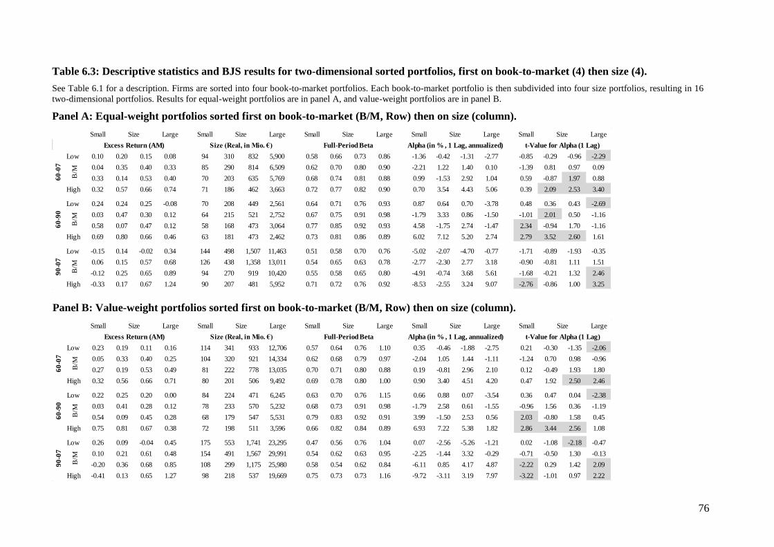
76
Panel B: Value-weight portfolios sorted first on book-to-market (B/M, Row) then on size (column).
Small Large Small Large Small Large Small Large Small Large
Low 0.23 0.19 0.11 0.16 114 341 933 12,706 0.57 0.64 0.76 1.10 0.35 -0.46 -1.88 -2.75 0.21 -0.30 -1.35 -2.06
0.05 0.33 0.40 0.25 104 320 921 14,334 0.62 0.68 0.79 0.97 -2.04 1.05 1.44 -1.11 -1.24 0.70 0.98 -0.96
0.27 0.19 0.53 0.49 81 222 778 13,035 0.70 0.71 0.80 0.88 0.19 -0.81 2.96 2.10 0.12 -0.49 1.93 1.80
High 0.32 0.56 0.66 0.71 80 201 506 9,492 0.69 0.78 0.80 1.00 0.90 3.40 4.51 4.20 0.47 1.92 2.50 2.46
Low 0.22 0.25 0.20 0.00 84 224 471 6,245 0.63 0.70 0.76 1.15 0.66 0.88 0.07 -3.54 0.36 0.47 0.04 -2.38
0.03 0.41 0.28 0.12 78 233 570 5,232 0.68 0.73 0.91 0.98 -1.79 2.58 0.61 -1.55 -0.96 1.56 0.36 -1.19
0.54 0.09 0.45 0.28 68 179 547 5,531 0.79 0.83 0.92 0.91 3.99 -1.50 2.53 0.56 2.03 -0.80 1.58 0.45
High 0.75 0.81 0.67 0.38 72 198 511 3,596 0.66 0.82 0.84 0.89 6.93 7.22 5.38 1.82 2.86 3.44 2.56 1.08
Low 0.26 0.09 -0.04 0.45 175 553 1,741 23,295 0.47 0.56 0.76 1.04 0.07 -2.56 -5.26 -1.21 0.02 -1.08 -2.18 -0.47
0.10 0.21 0.61 0.48 154 491 1,567 29,991 0.54 0.62 0.63 0.95 -2.25 -1.44 3.32 -0.29 -0.71 -0.50 1.30 -0.13
-0.20 0.36 0.68 0.85 108 299 1,175 25,980 0.58 0.54 0.62 0.84 -6.11 0.85 4.17 4.87 -2.22 0.29 1.42 2.09
High -0.41 0.13 0.65 1.27 98 218 537 19,669 0.75 0.73 0.73 1.16 -9.72 -3.11 3.19 7.97 -3.22 -1.01 0.97 2.22
60
-07
60
-90
90
-07
Size Size
t-Value for Alpha (1 Lag)
B/M
B/M
Alpha (in % , 1 Lag, annualized)
B/M
Size
Full-Period Beta
Size Size
Excess Return (AM) Size (Real, in Mio. €)
Table 6.3: Descriptive statistics and BJS results for two-dimensional sorted portfolios, first on book-to-market (4) then size (4).
See Table 6.1 for a description. Firms are sorted into four book-to-market portfolios. Each book-to-market portfolio is then subdivided into four size portfolios, resulting in 16
two-dimensional portfolios. Results for equal-weight portfolios are in panel A, and value-weight portfolios are in panel B.
Panel A: Equal-weight portfolios sorted first on book-to-market (B/M, Row) then on size (column).
Small Large Small Large Small Large Small Large Small Large
Low 0.10 0.20 0.15 0.08 94 310 832 5,900 0.58 0.66 0.73 0.86 -1.36 -0.42 -1.31 -2.77 -0.85 -0.29 -0.96 -2.29
0.04 0.35 0.40 0.33 85 290 814 6,509 0.62 0.70 0.80 0.90 -2.21 1.22 1.40 0.10 -1.39 0.81 0.97 0.09
0.33 0.14 0.53 0.40 70 203 635 5,769 0.68 0.74 0.81 0.88 0.99 -1.53 2.92 1.04 0.59 -0.87 1.97 0.88
High 0.32 0.57 0.66 0.74 71 186 462 3,663 0.72 0.77 0.82 0.90 0.70 3.54 4.43 5.06 0.39 2.09 2.53 3.40
Low 0.24 0.24 0.25 -0.08 70 208 449 2,561 0.64 0.71 0.76 0.93 0.87 0.64 0.70 -3.78 0.48 0.36 0.43 -2.69
0.03 0.47 0.30 0.12 64 215 521 2,752 0.67 0.75 0.91 0.98 -1.79 3.33 0.86 -1.50 -1.01 2.01 0.50 -1.16
0.58 0.07 0.47 0.12 58 168 473 3,064 0.77 0.85 0.92 0.93 4.58 -1.75 2.74 -1.47 2.34 -0.94 1.70 -1.16
High 0.69 0.80 0.66 0.46 63 181 473 2,462 0.73 0.81 0.86 0.89 6.02 7.12 5.20 2.74 2.79 3.52 2.60 1.61
Low -0.15 0.14 -0.02 0.34 144 498 1,507 11,463 0.51 0.58 0.70 0.76 -5.02 -2.07 -4.70 -0.77 -1.71 -0.89 -1.93 -0.35
0.06 0.15 0.57 0.68 126 438 1,358 13,011 0.54 0.65 0.63 0.78 -2.77 -2.30 2.77 3.18 -0.90 -0.81 1.11 1.51
-0.12 0.25 0.65 0.89 94 270 919 10,420 0.55 0.58 0.65 0.80 -4.91 -0.74 3.68 5.61 -1.68 -0.21 1.32 2.46
High -0.33 0.17 0.67 1.24 90 207 481 5,952 0.71 0.72 0.76 0.92 -8.53 -2.55 3.24 9.07 -2.76 -0.86 1.00 3.25
60
-90
90
-07
60
-07
Size Size
t-Value for Alpha (1 Lag)Alpha (in % , 1 Lag, annualized)
B/M
B/M
B/M
Excess Return (AM) Size (Real, in Mio. €) Full-Period Beta
Size Size Size
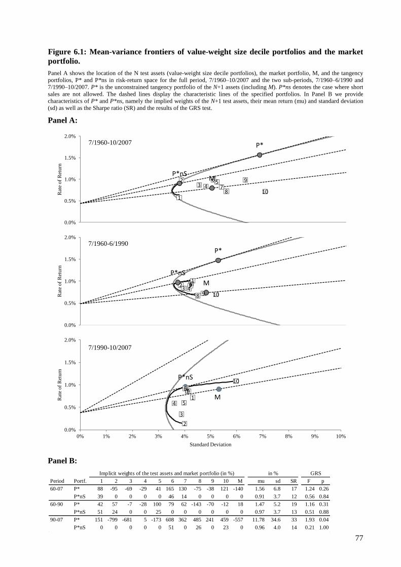
77
Figure 6.1: Mean-variance frontiers of value-weight size decile portfolios and the market
portfolio.
Panel A shows the location of the N test assets (value-weight size decile portfolios), the market portfolio, M, and the tangency
portfolios, P* and P*ns in risk-return space for the full period, 7/1960–10/2007 and the two sub-periods, 7/1960–6/1990 and
7/1990–10/2007. P* is the unconstrained tangency portfolio of the N+1 assets (including M). P*ns denotes the case where short
sales are not allowed. The dashed lines display the characteristic lines of the specified portfolios. In Panel B we provide
characteristics of P* and P*ns, namely the implied weights of the N+1 test assets, their mean return (mu) and standard deviation
(sd) as well as the Sharpe ratio (SR) and the results of the GRS test.
Panel A:
Panel B:
1
2 3 4
5 6 7
8
9
10
M
P*
P*nS
0.0%
0.5%
1.0%
1.5%
2.0%
Rat
e of
Ret
urn
7/1960-10/2007
1 2 3 4
5 6 7
8 9 10
M
P*
P*nS
0.0%
0.5%
1.0%
1.5%
2.0%
Rat
e of
Ret
urn
7/1960-6/1990
M
P*nS
1
2
3
4 5
6 7 8 9
10
0.0%
0.5%
1.0%
1.5%
2.0%
0% 1% 2% 3% 4% 5% 6% 7% 8% 9% 10%
Rat
e of
Ret
urn
Standard Deviation
7/1990-10/2007
Implicit weights of the test assets and market portfolio (in %)
Period Portf. 1 2 3 4 5 6 7 8 9 10 M mu sd SR F p
60-07 P* 88 -95 -69 -29 41 165 130 -75 -38 121 -140 1.56 6.8 17 1.24 0.26
P*nS 39 0 0 0 0 46 14 0 0 0 0 0.91 3.7 12 0.56 0.84
60-90 P* 42 57 -7 -28 100 79 62 -143 -70 -12 18 1.47 5.2 19 1.16 0.31
P*nS 51 24 0 0 25 0 0 0 0 0 0 0.97 3.7 13 0.51 0.88
90-07 P* 151 -799 -681 5 -173 608 362 485 241 459 -557 11.78 34.6 33 1.93 0.04
P*nS 0 0 0 0 0 51 0 26 0 23 0 0.96 4.0 14 0.21 1.00
in % GRS
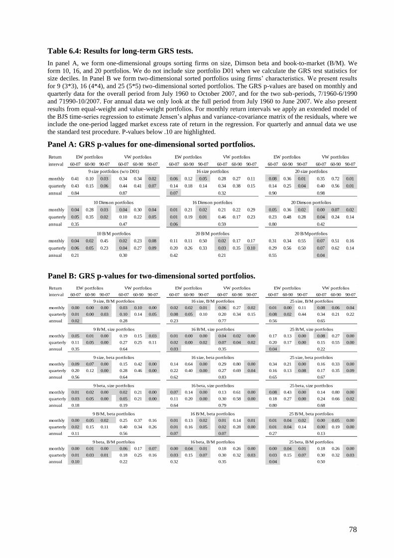
78
Panel B: GRS p-values for two-dimensional sorted portfolios.
Return
interval 60-07 60-90 90-07 60-07 60-90 90-07 60-07 60-90 90-07 60-07 60-90 90-07 60-07 60-90 90-07 60-07 60-90 90-07
monthly 0.00 0.00 0.00 0.03 0.10 0.00 0.02 0.02 0.01 0.06 0.27 0.02 0.01 0.00 0.11 0.08 0.06 0.04
quarterly 0.01 0.00 0.03 0.10 0.14 0.05 0.08 0.05 0.10 0.20 0.34 0.15 0.08 0.02 0.44 0.34 0.21 0.22
annual 0.02 0.28 0.23 0.77 0.56 0.65
monthly 0.05 0.01 0.00 0.19 0.15 0.03 0.01 0.00 0.00 0.04 0.02 0.00 0.17 0.13 0.00 0.08 0.27 0.00
quarterly 0.11 0.05 0.00 0.27 0.25 0.11 0.02 0.00 0.02 0.07 0.04 0.02 0.20 0.17 0.00 0.15 0.55 0.00
annual 0.35 0.64 0.03 0.35 0.04 0.22
monthly 0.09 0.07 0.00 0.15 0.42 0.00 0.14 0.64 0.00 0.29 0.80 0.00 0.34 0.21 0.00 0.16 0.33 0.00
quarterly 0.20 0.12 0.00 0.28 0.46 0.00 0.22 0.40 0.00 0.27 0.69 0.04 0.16 0.13 0.08 0.17 0.35 0.09
annual 0.56 0.64 0.62 0.83 0.65 0.67
monthly 0.01 0.02 0.00 0.02 0.21 0.00 0.07 0.14 0.00 0.13 0.61 0.00 0.08 0.43 0.00 0.14 0.80 0.00
quarterly 0.03 0.05 0.00 0.05 0.21 0.00 0.11 0.20 0.00 0.30 0.58 0.00 0.18 0.27 0.00 0.24 0.66 0.02
annual 0.18 0.19 0.64 0.79 0.80 0.68
monthly 0.00 0.05 0.02 0.25 0.37 0.16 0.01 0.13 0.02 0.01 0.14 0.01 0.01 0.04 0.02 0.00 0.05 0.00
quarterly 0.02 0.15 0.11 0.40 0.34 0.26 0.01 0.16 0.05 0.02 0.28 0.00 0.01 0.04 0.14 0.00 0.19 0.00
annual 0.11 0.56 0.07 0.07 0.27 0.13
monthly 0.00 0.01 0.00 0.06 0.17 0.07 0.00 0.04 0.01 0.18 0.26 0.00 0.00 0.04 0.01 0.18 0.26 0.00
quarterly 0.01 0.03 0.01 0.18 0.25 0.16 0.03 0.15 0.07 0.30 0.32 0.03 0.03 0.15 0.07 0.30 0.32 0.03
annual 0.10 0.22 0.32 0.35 0.04 0.50
9 size, beta portfolios
9 beta, size portfolios 16 beta, size portfolios 25 beta, size portfolios
16 size, beta portfolios 25 size, beta portfolios
9 B/M, size portfolios 16 B/M, size portfolios 25 B/M, size portfolios
9 beta, B/M portfolios 16 beta, B/M portfolios 25 beta, B/M portfolios
EW portfolios VW portfolios EW portfolios VW portfolios EW portfolios VW portfolios
9 B/M, beta portfolios 16 B/M, beta portfolios 25 B/M, beta portfolios
9 size, B/M portfolios 16 size, B/M portfolios 25 size, B/M portfolios
Table 6.4: Results for long-term GRS tests.
In panel A, we form one-dimensional groups sorting firms on size, Dimson beta and book-to-market (B/M). We
form 10, 16, and 20 portfolios. We do not include size portfolio D01 when we calculate the GRS test statistics for
size deciles. In Panel B we form two-dimensional sorted portfolios using firms’ characteristics. We present results
for 9 (3*3), 16 (4*4), and 25 (5*5) two-dimensional sorted portfolios. The GRS p-values are based on monthly and
quarterly data for the overall period from July 1960 to October 2007, and for the two sub-periods, 7/1960-6/1990
and 71990-10/2007. For annual data we only look at the full period from July 1960 to June 2007. We also present
results from equal-weight and value-weight portfolios. For monthly return intervals we apply an extended model of
the BJS time-series regression to estimate Jensen’s alphas and variance-covariance matrix of the residuals, where we
include the one-period lagged market excess rate of return in the regression. For quarterly and annual data we use
the standard test procedure. P-values below .10 are highlighted.
Panel A: GRS p-values for one-dimensional sorted portfolios.
Return
interval 60-07 60-90 90-07 60-07 60-90 90-07 60-07 60-90 90-07 60-07 60-90 90-07 60-07 60-90 90-07 60-07 60-90 90-07
monthly 0.41 0.10 0.03 0.34 0.34 0.02 0.06 0.12 0.05 0.28 0.27 0.11 0.08 0.36 0.01 0.35 0.72 0.01
quarterly 0.43 0.15 0.06 0.44 0.41 0.07 0.14 0.18 0.14 0.34 0.38 0.15 0.14 0.25 0.04 0.40 0.56 0.01
annual 0.84 0.87 0.07 0.32 0.90 0.98
monthly 0.04 0.28 0.03 0.04 0.30 0.04 0.01 0.21 0.02 0.21 0.22 0.29 0.05 0.36 0.02 0.00 0.07 0.02
quarterly 0.05 0.35 0.02 0.10 0.22 0.05 0.01 0.19 0.01 0.46 0.17 0.23 0.23 0.48 0.28 0.04 0.24 0.14
annual 0.35 0.47 0.06 0.59 0.80 0.42
monthly 0.04 0.02 0.45 0.02 0.23 0.08 0.11 0.11 0.50 0.02 0.17 0.17 0.31 0.34 0.55 0.07 0.51 0.16
quarterly 0.06 0.05 0.23 0.04 0.27 0.09 0.20 0.26 0.33 0.03 0.35 0.10 0.29 0.56 0.50 0.07 0.62 0.14
annual 0.21 0.30 0.42 0.21 0.55 0.04
10 Dimson portfolios 16 Dimson portfolios 20 Dimson portfolios
10 B/M portfolios 20 B/M portfolios 20 B/Mportfolios
EW portfolios VW portfolios
20 size portfolios
EW portfolios VW portfolios EW portfolios VW portfolios
9 size portfolios (w/o D01) 16 size portfolios
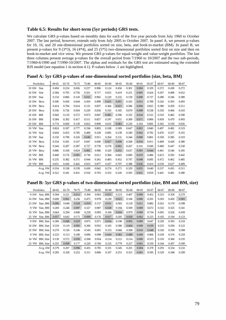
79
Table 6.5: Results for short-term (5yr periods) GRS tests.
We calculate GRS p-values based on monthly data for each of the five year periods from July 1960 to October
2007. The last period, however, extends only from July 2005 to October 2007. In panel A, we present p-values
for 10, 16, and 20 one-dimensional portfolios sorted on size, beta, and book-to-market (BM). In panel B, we
present p-values for 9 (3*3), 16 (4*4), and 25 (5*5) two-dimensional portfolios sorted first on size and then on
book-to-market and vice versa. We present GRS p-values for equal-weight and value-weight portfolios. The last
three columns present average p-values for the overall period from 7/1960 to 10/2007 and the two sub-periods,
7/1960-6/1990 and 7/1990-10/2007. The alphas and residuals for the GRS test are estimated using the extended
BJS model (see equation 1 in section 4.1). P-values below .1 are highlighted.
Panel A: 5yr GRS p-values of one-dimensional sorted portfolios (size, beta, BM)
60-65 65-70 70-75 75-80 80-85 85-90 90-95 95-00 00-05 05-07 60-07 60-90 90-07
10 EW Size 0.494 0.224 0.656 0.227 0.906 0.124 0.456 0.301 0.004 0.329 0.372 0.438 0.272
16 EW Size 0.584 0.705 0.756 0.501 0.717 0.652 0.419 0.221 0.005 0.424 0.267 0.498 0.652
20 EW Size 0.134 0.866 0.120 0.032 0.965 0.220 0.232 0.159 0.000 0.727 0.280 0.346 0.389
10 EW Beta 0.506 0.436 0.644 0.450 0.898 0.025 0.001 0.165 0.015 0.788 0.242 0.393 0.493
16 EW Beta 0.414 0.704 0.614 0.131 0.837 0.366 0.021 0.586 0.094 0.822 0.380 0.459 0.511
20 EW Beta 0.556 0.726 0.934 0.220 0.656 0.165 0.185 0.670 0.008 0.538 0.350 0.466 0.543
10 EW BM 0.943 0.119 0.572 0.973 0.847 0.085 0.396 0.332 0.034 0.515 0.319 0.482 0.590
16 EW BM 0.584 0.392 0.417 0.511 0.857 0.197 0.651 0.309 0.071 0.806 0.459 0.479 0.493
20 EW BM 0.774 0.669 0.139 0.822 0.899 0.632 0.083 0.220 0.264 0.892 0.365 0.539 0.656
10 VW Size 0.824 0.187 0.777 0.194 0.803 0.108 0.589 0.647 0.001 0.840 0.497 0.482 0.519
16 VW Size 0.604 0.453 0.785 0.489 0.328 0.685 0.238 0.349 0.042 0.792 0.476 0.557 0.355
20 VW Size 0.150 0.709 0.226 0.049 0.911 0.264 0.131 0.344 0.000 0.801 0.358 0.385 0.319
10 VW Beta 0.554 0.281 0.167 0.847 0.690 0.027 0.008 0.568 0.034 0.911 0.409 0.428 0.380
16 VW Beta 0.344 0.287 0.287 0.727 0.759 0.278 0.002 0.267 0.101 0.949 0.400 0.447 0.330
20 VW Beta 0.886 0.169 0.824 0.081 0.986 0.329 0.055 0.637 0.003 0.044 0.401 0.546 0.185
10 VW BM 0.449 0.176 0.005 0.730 0.611 0.384 0.665 0.600 0.019 0.486 0.413 0.393 0.442
16 VW BM 0.235 0.382 0.371 0.944 0.361 0.483 0.452 0.747 0.048 0.695 0.472 0.462 0.485
20 VW BM 0.651 0.430 0.442 0.923 0.877 0.437 0.797 0.388 0.036 0.414 0.539 0.627 0.409
0.554 0.538 0.539 0.430 0.842 0.274 0.271 0.329 0.055 0.649 0.337 0.455 0.511
0.522 0.341 0.431 0.554 0.703 0.333 0.326 0.505 0.031 0.659 0.441 0.481 0.380
Portfolios
Avg. VW
Avg. EW
Panel B: 5yr GRS p-values of two-dimensional sorted portfolios (size, BM and BM, size)
60-65 65-70 70-75 75-80 80-85 85-90 90-95 95-00 00-05 05-07 60-07 60-90 90-07
9 EW Size, BM 0.504 0.221 0.012 0.394 0.963 0.053 0.223 0.407 0.000 0.452 0.323 0.358 0.270
16 EW Size, BM 0.699 0.061 0.256 0.475 0.978 0.230 0.023 0.106 0.000 0.201 0.303 0.450 0.083
25 EW Size, BM 0.096 0.649 0.028 0.059 0.157 0.031 0.583 0.118 0.011 0.882 0.261 0.170 0.398
9 VW Size, BM 0.269 0.246 0.097 0.327 0.987 0.028 0.184 0.509 0.000 0.672 0.332 0.325 0.341
16 VW Size, BM 0.664 0.294 0.840 0.258 0.993 0.106 0.044 0.979 0.000 0.734 0.491 0.526 0.439
25 VW Size, BM 0.057 0.642 0.171 0.099 0.176 0.017 0.205 0.058 0.002 0.225 0.165 0.194 0.123
9 EW BM, Size 0.384 0.068 0.029 0.875 0.971 0.034 0.190 0.005 0.000 0.647 0.320 0.393 0.210
16 EW BM, Size 0.319 0.119 0.005 0.266 0.952 0.105 0.386 0.064 0.000 0.039 0.225 0.294 0.122
25 EW BM, Size 0.270 0.126 0.246 0.543 0.691 0.153 0.666 0.508 0.010 0.048 0.326 0.338 0.308
9 VW BM, Size 0.223 0.113 0.180 0.696 0.998 0.044 0.083 0.088 0.000 0.866 0.329 0.376 0.259
16 VW BM, Size 0.130 0.572 0.050 0.268 0.924 0.214 0.212 0.214 0.000 0.515 0.310 0.360 0.235
25 VW BM, Size 0.355 0.099 0.177 0.220 0.760 0.235 0.779 0.257 0.001 0.559 0.344 0.307 0.399
0.379 0.207 0.096 0.435 0.785 0.101 0.345 0.201 0.004 0.378 0.293 0.334 0.232
0.283 0.328 0.252 0.311 0.806 0.107 0.251 0.351 0.001 0.595 0.329 0.348 0.299
Avg. EW
Avg. VW
Portfolios

80
Table 6.6: Results for cross-sectional FM regressions with one independent variable for one-dimensional sorted portfolios.
The table presents average intercepts (annualized alphas in %) and slopes on firm/portfolio characteristics (also annualized in%) from cross-sectional FM regressions of excess
returns on size, book-to-market, or beta. The independent variable in the regression matches the grouping criterion. We look at individual firms and at portfolios grouped by
size, book-to-market, and beta. Specification: We use monthly (M), quarterly (Q) and annual (A) excess rates of return as dependent variable in the regressions. We look at
individual firms, but also form 10, 16, and 20 portfolios. We apply different beta estimation procedures for our beta groups. We use monthly (MFP), quarterly (QFP), and
annual (AFP) full-period betas. In addition we use 5yr rolling betas on a monthly (MRB) and quarterly (QRB) basis. Monthly betas are estimated according to Dimson (1979)
using the lagged market excess return. In firm level regressions á la Fama/French (1992) we assign portfolios’ full period betas to the firms in the portfolio. MFP10 for example
indicates that we form 10 portfolios and assign portfolios’ full period beta to every firm in the portfolio. Results for equal-weight portfolios are presented on the left side of the
table, and for value-weight portfolios on the right side. We look at the overall period from 7/1960 to 10/2007, as well as two sub-periods, 7/1960-6/1990 and 7/1990-10/2007.
The t-values for the intercepts and slopes are presented in parentheses. T-values above/below 1.96 are highlighted.
M firms 0.64 (0.27) 0.45 (1.17) 6.74 (2.47) -0.56 (-1.20) -9.93 (-2.41) 2.19 (3.47) 0.64 (0.27) 0.45 (1.17) 6.74 (2.47) -0.56 (-1.20) -9.93 (-2.41) 2.19 (3.47)
Q firms 0.37 (0.13) 0.54 (1.31) 7.00 (2.21) -0.56 (-1.21) -11.16 (-2.12) 2.45 (3.35) 0.37 (0.13) 0.54 (1.31) 7.00 (2.21) -0.56 (-1.21) -11.16 (-2.12) 2.45 (3.35)
M 10 3.61 (1.68) 0.00 (0.00) 7.74 (3.01) -0.73 (-1.64) -3.55 (-0.94) 1.27 (2.21) 2.89 (1.30) 0.13 (0.35) 7.10 (2.64) -0.59 (-1.29) -4.40 (-1.14) 1.37 (2.24)
M 16 0.56 (0.24) 0.46 (1.21) 6.85 (2.46) -0.57 (-1.21) -10.33 (-2.49) 2.25 (3.55) 1.15 (0.49) 0.36 (0.94) 6.18 (2.21) -0.46 (-0.95) -7.57 (-1.84) 1.79 (2.83)
M 20 0.70 (0.30) 0.44 (1.13) 7.00 (2.48) -0.60 (-1.24) -10.20 (-2.45) 2.23 (3.54) 1.10 (0.47) 0.38 (0.98) 6.18 (2.19) -0.46 (-0.93) -7.70 (-1.89) 1.83 (2.90)
Q 10 4.22 (1.54) -0.04 (-0.12) 8.30 (2.61) -0.79 (-1.77) -2.87 (-0.57) 1.25 (1.94) 3.33 (1.20) 0.11 (0.28) 7.58 (2.35) -0.63 (-1.43) -4.07 (-0.82) 1.39 (2.02)
Q 16 0.90 (0.32) 0.46 (1.16) 7.25 (2.30) -0.59 (-1.31) -10.16 (-1.96) 2.29 (3.26) 1.46 (0.52) 0.36 (0.90) 6.59 (2.09) -0.49 (-1.06) -7.46 (-1.44) 1.84 (2.55)
Q 20 1.06 (0.37) 0.43 (1.07) 7.42 (2.31) -0.63 (-1.34) -10.01 (-1.91) 2.27 (3.21) 1.39 (0.50) 0.38 (0.94) 6.57 (2.06) -0.48 (-1.02) -7.62 (-1.49) 1.88 (2.65)
A 10 5.35 (1.55) -0.15 (-0.32) 9.00 (2.17) -0.83 (-1.33) -1.09 (-0.18) 1.06 (1.74) 4.20 (1.24) 0.06 (0.13) 8.07 (1.95) -0.62 (-0.99) -2.64 (-0.47) 1.26 (1.99)
A 16 1.85 (0.51) 0.39 (0.78) 7.89 (1.86) -0.62 (-0.98) -8.80 (-1.50) 2.17 (3.69) 2.42 (0.69) 0.29 (0.59) 7.13 (1.68) -0.50 (-0.77) -5.89 (-1.01) 1.69 (2.61)
A 20 2.14 (0.59) 0.34 (0.68) 8.20 (1.86) -0.68 (-1.04) -8.56 (-1.50) 2.14 (3.85) 2.38 (0.67) 0.32 (0.63) 7.22 (1.64) -0.50 (-0.75) -6.15 (-1.09) 1.76 (2.83)
M firms 5.56 (2.68) 2.98 (3.74) 6.13 (2.38) 3.58 (3.19) 4.56 (1.31) 1.94 (1.99) 5.56 (2.68) 2.98 (3.74) 6.13 (2.38) 3.58 (3.19) 4.56 (1.31) 1.94 (1.99)
Q firms 5.86 (2.32) 3.05 (3.39) 6.53 (2.14) 3.90 (3.17) 4.69 (1.04) 1.58 (1.29) 5.86 (2.32) 3.05 (3.39) 6.53 (2.14) 3.90 (3.17) 4.69 (1.04) 1.58 (1.29)
M 10 5.75 (2.76) 3.43 (4.02) 6.42 (2.49) 4.22 (3.53) 4.59 (1.30) 2.06 (1.93) 7.62 (3.12) 4.64 (3.62) 5.30 (1.86) 4.15 (2.59) 11.63 (2.60) 5.49 (2.56)
M 16 5.65 (2.71) 3.28 (3.83) 6.34 (2.46) 4.06 (3.40) 4.45 (1.26) 1.94 (1.77) 7.40 (3.11) 4.53 (3.78) 5.21 (1.84) 4.17 (2.78) 11.21 (2.63) 5.17 (2.57)
M 20 5.70 (2.75) 3.36 (3.85) 6.40 (2.49) 4.19 (3.41) 4.47 (1.28) 1.92 (1.80) 7.43 (3.15) 4.54 (3.82) 5.52 (1.96) 4.25 (2.82) 10.72 (2.56) 5.05 (2.61)
Q 10 6.26 (2.46) 3.67 (3.82) 6.83 (2.24) 4.43 (3.36) 5.25 (1.15) 2.34 (1.81) 8.10 (2.85) 4.77 (3.53) 5.70 (1.74) 4.38 (2.62) 12.29 (2.31) 5.45 (2.36)
Q 16 6.16 (2.42) 3.54 (3.62) 6.77 (2.22) 4.29 (3.23) 5.11 (1.12) 2.22 (1.66) 7.90 (2.81) 4.73 (3.58) 5.64 (1.72) 4.50 (2.73) 11.81 (2.28) 5.13 (2.31)
Q 20 6.20 (2.44) 3.62 (3.69) 6.80 (2.24) 4.42 (3.27) 5.14 (1.13) 2.23 (1.71) 7.91 (2.87) 4.71 (3.66) 5.94 (1.83) 4.52 (2.76) 11.34 (2.25) 5.04 (2.40)
A 10 6.82 (2.31) 4.00 (3.53) 7.40 (2.05) 4.83 (3.23) 5.78 (1.11) 2.54 (1.51) 8.41 (2.62) 4.96 (2.83) 6.12 (1.59) 4.45 (2.22) 12.44 (2.16) 5.87 (1.73)
A 16 6.72 (2.28) 3.87 (3.34) 7.34 (2.04) 4.69 (3.08) 5.63 (1.07) 2.44 (1.38) 8.25 (2.59) 4.98 (2.92) 6.03 (1.61) 4.58 (2.39) 12.16 (2.09) 5.69 (1.70)
A 20 6.73 (2.30) 3.93 (3.34) 7.34 (2.05) 4.78 (3.05) 5.66 (1.09) 2.43 (1.42) 8.30 (2.65) 5.04 (3.12) 6.36 (1.71) 4.61 (2.40) 11.74 (2.05) 5.79 (1.95)
Alpha B/M Alpha B/M
Size Alpha
Value-weight size portfolios
7/1960-10/2007 7/1960-6/1990 7/1990-10/2007
Size
Alpha B/MAlpha B/M Alpha
Equal-weight size portfolios
7/1960-6/1990 7/1990-10/2007
Equal-weight book-to-market portfolios Value-weight book-to-market portfolios
Size
B/MB/MAlpha
Specification Alpha Size Alpha
7/1960-10/2007
Alpha Size Alpha Size Alpha
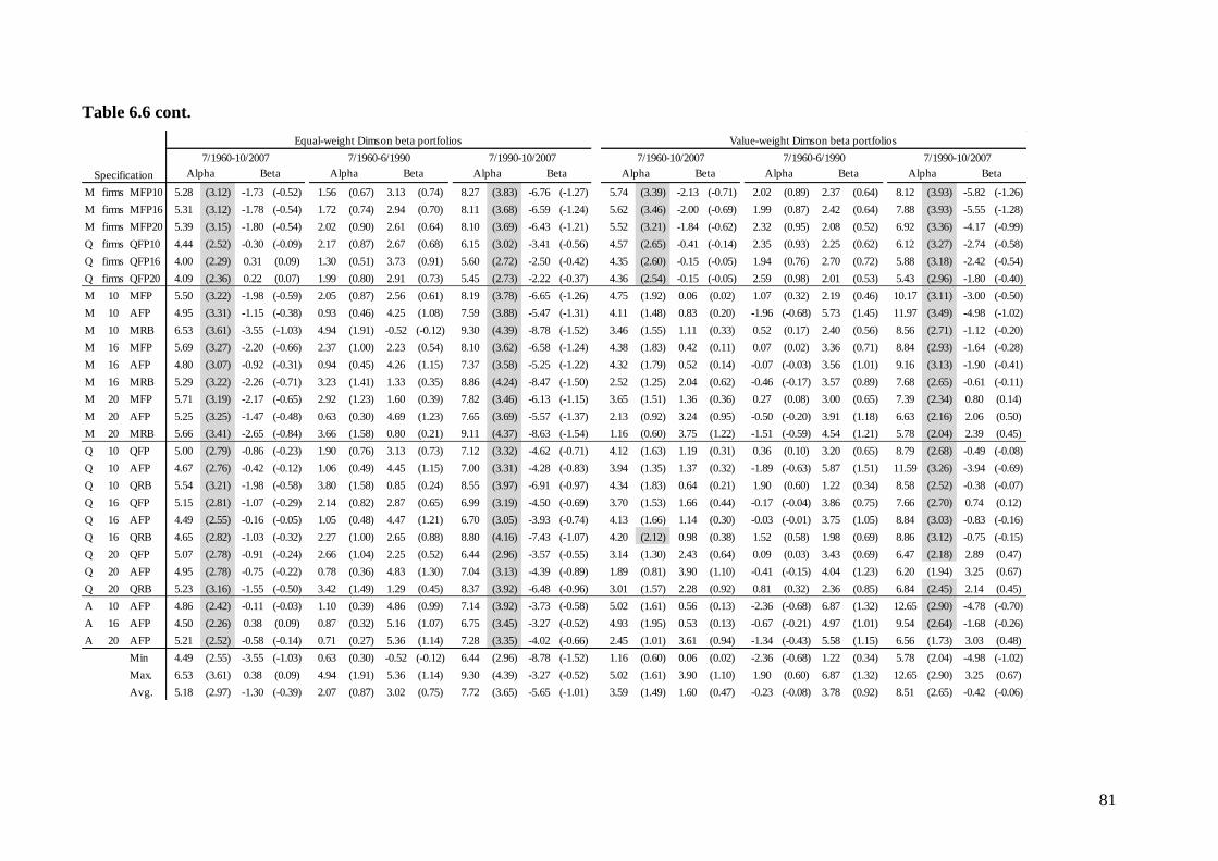
81
Table 6.6 cont.
M firms MFP10 5.28 (3.12) -1.73 (-0.52) 1.56 (0.67) 3.13 (0.74) 8.27 (3.83) -6.76 (-1.27) 5.74 (3.39) -2.13 (-0.71) 2.02 (0.89) 2.37 (0.64) 8.12 (3.93) -5.82 (-1.26)
M firms MFP16 5.31 (3.12) -1.78 (-0.54) 1.72 (0.74) 2.94 (0.70) 8.11 (3.68) -6.59 (-1.24) 5.62 (3.46) -2.00 (-0.69) 1.99 (0.87) 2.42 (0.64) 7.88 (3.93) -5.55 (-1.28)
M firms MFP20 5.39 (3.15) -1.80 (-0.54) 2.02 (0.90) 2.61 (0.64) 8.10 (3.69) -6.43 (-1.21) 5.52 (3.21) -1.84 (-0.62) 2.32 (0.95) 2.08 (0.52) 6.92 (3.36) -4.17 (-0.99)
Q firms QFP10 4.44 (2.52) -0.30 (-0.09) 2.17 (0.87) 2.67 (0.68) 6.15 (3.02) -3.41 (-0.56) 4.57 (2.65) -0.41 (-0.14) 2.35 (0.93) 2.25 (0.62) 6.12 (3.27) -2.74 (-0.58)
Q firms QFP16 4.00 (2.29) 0.31 (0.09) 1.30 (0.51) 3.73 (0.91) 5.60 (2.72) -2.50 (-0.42) 4.35 (2.60) -0.15 (-0.05) 1.94 (0.76) 2.70 (0.72) 5.88 (3.18) -2.42 (-0.54)
Q firms QFP20 4.09 (2.36) 0.22 (0.07) 1.99 (0.80) 2.91 (0.73) 5.45 (2.73) -2.22 (-0.37) 4.36 (2.54) -0.15 (-0.05) 2.59 (0.98) 2.01 (0.53) 5.43 (2.96) -1.80 (-0.40)
M 10 MFP 5.50 (3.22) -1.98 (-0.59) 2.05 (0.87) 2.56 (0.61) 8.19 (3.78) -6.65 (-1.26) 4.75 (1.92) 0.06 (0.02) 1.07 (0.32) 2.19 (0.46) 10.17 (3.11) -3.00 (-0.50)
M 10 AFP 4.95 (3.31) -1.15 (-0.38) 0.93 (0.46) 4.25 (1.08) 7.59 (3.88) -5.47 (-1.31) 4.11 (1.48) 0.83 (0.20) -1.96 (-0.68) 5.73 (1.45) 11.97 (3.49) -4.98 (-1.02)
M 10 MRB 6.53 (3.61) -3.55 (-1.03) 4.94 (1.91) -0.52 (-0.12) 9.30 (4.39) -8.78 (-1.52) 3.46 (1.55) 1.11 (0.33) 0.52 (0.17) 2.40 (0.56) 8.56 (2.71) -1.12 (-0.20)
M 16 MFP 5.69 (3.27) -2.20 (-0.66) 2.37 (1.00) 2.23 (0.54) 8.10 (3.62) -6.58 (-1.24) 4.38 (1.83) 0.42 (0.11) 0.07 (0.02) 3.36 (0.71) 8.84 (2.93) -1.64 (-0.28)
M 16 AFP 4.80 (3.07) -0.92 (-0.31) 0.94 (0.45) 4.26 (1.15) 7.37 (3.58) -5.25 (-1.22) 4.32 (1.79) 0.52 (0.14) -0.07 (-0.03) 3.56 (1.01) 9.16 (3.13) -1.90 (-0.41)
M 16 MRB 5.29 (3.22) -2.26 (-0.71) 3.23 (1.41) 1.33 (0.35) 8.86 (4.24) -8.47 (-1.50) 2.52 (1.25) 2.04 (0.62) -0.46 (-0.17) 3.57 (0.89) 7.68 (2.65) -0.61 (-0.11)
M 20 MFP 5.71 (3.19) -2.17 (-0.65) 2.92 (1.23) 1.60 (0.39) 7.82 (3.46) -6.13 (-1.15) 3.65 (1.51) 1.36 (0.36) 0.27 (0.08) 3.00 (0.65) 7.39 (2.34) 0.80 (0.14)
M 20 AFP 5.25 (3.25) -1.47 (-0.48) 0.63 (0.30) 4.69 (1.23) 7.65 (3.69) -5.57 (-1.37) 2.13 (0.92) 3.24 (0.95) -0.50 (-0.20) 3.91 (1.18) 6.63 (2.16) 2.06 (0.50)
M 20 MRB 5.66 (3.41) -2.65 (-0.84) 3.66 (1.58) 0.80 (0.21) 9.11 (4.37) -8.63 (-1.54) 1.16 (0.60) 3.75 (1.22) -1.51 (-0.59) 4.54 (1.21) 5.78 (2.04) 2.39 (0.45)
Q 10 QFP 5.00 (2.79) -0.86 (-0.23) 1.90 (0.76) 3.13 (0.73) 7.12 (3.32) -4.62 (-0.71) 4.12 (1.63) 1.19 (0.31) 0.36 (0.10) 3.20 (0.65) 8.79 (2.68) -0.49 (-0.08)
Q 10 AFP 4.67 (2.76) -0.42 (-0.12) 1.06 (0.49) 4.45 (1.15) 7.00 (3.31) -4.28 (-0.83) 3.94 (1.35) 1.37 (0.32) -1.89 (-0.63) 5.87 (1.51) 11.59 (3.26) -3.94 (-0.69)
Q 10 QRB 5.54 (3.21) -1.98 (-0.58) 3.80 (1.58) 0.85 (0.24) 8.55 (3.97) -6.91 (-0.97) 4.34 (1.83) 0.64 (0.21) 1.90 (0.60) 1.22 (0.34) 8.58 (2.52) -0.38 (-0.07)
Q 16 QFP 5.15 (2.81) -1.07 (-0.29) 2.14 (0.82) 2.87 (0.65) 6.99 (3.19) -4.50 (-0.69) 3.70 (1.53) 1.66 (0.44) -0.17 (-0.04) 3.86 (0.75) 7.66 (2.70) 0.74 (0.12)
Q 16 AFP 4.49 (2.55) -0.16 (-0.05) 1.05 (0.48) 4.47 (1.21) 6.70 (3.05) -3.93 (-0.74) 4.13 (1.66) 1.14 (0.30) -0.03 (-0.01) 3.75 (1.05) 8.84 (3.03) -0.83 (-0.16)
Q 16 QRB 4.65 (2.82) -1.03 (-0.32) 2.27 (1.00) 2.65 (0.88) 8.80 (4.16) -7.43 (-1.07) 4.20 (2.12) 0.98 (0.38) 1.52 (0.58) 1.98 (0.69) 8.86 (3.12) -0.75 (-0.15)
Q 20 QFP 5.07 (2.78) -0.91 (-0.24) 2.66 (1.04) 2.25 (0.52) 6.44 (2.96) -3.57 (-0.55) 3.14 (1.30) 2.43 (0.64) 0.09 (0.03) 3.43 (0.69) 6.47 (2.18) 2.89 (0.47)
Q 20 AFP 4.95 (2.78) -0.75 (-0.22) 0.78 (0.36) 4.83 (1.30) 7.04 (3.13) -4.39 (-0.89) 1.89 (0.81) 3.90 (1.10) -0.41 (-0.15) 4.04 (1.23) 6.20 (1.94) 3.25 (0.67)
Q 20 QRB 5.23 (3.16) -1.55 (-0.50) 3.42 (1.49) 1.29 (0.45) 8.37 (3.92) -6.48 (-0.96) 3.01 (1.57) 2.28 (0.92) 0.81 (0.32) 2.36 (0.85) 6.84 (2.45) 2.14 (0.45)
A 10 AFP 4.86 (2.42) -0.11 (-0.03) 1.10 (0.39) 4.86 (0.99) 7.14 (3.92) -3.73 (-0.58) 5.02 (1.61) 0.56 (0.13) -2.36 (-0.68) 6.87 (1.32) 12.65 (2.90) -4.78 (-0.70)
A 16 AFP 4.50 (2.26) 0.38 (0.09) 0.87 (0.32) 5.16 (1.07) 6.75 (3.45) -3.27 (-0.52) 4.93 (1.95) 0.53 (0.13) -0.67 (-0.21) 4.97 (1.01) 9.54 (2.64) -1.68 (-0.26)
A 20 AFP 5.21 (2.52) -0.58 (-0.14) 0.71 (0.27) 5.36 (1.14) 7.28 (3.35) -4.02 (-0.66) 2.45 (1.01) 3.61 (0.94) -1.34 (-0.43) 5.58 (1.15) 6.56 (1.73) 3.03 (0.48)
Min 4.49 (2.55) -3.55 (-1.03) 0.63 (0.30) -0.52 (-0.12) 6.44 (2.96) -8.78 (-1.52) 1.16 (0.60) 0.06 (0.02) -2.36 (-0.68) 1.22 (0.34) 5.78 (2.04) -4.98 (-1.02)
Max. 6.53 (3.61) 0.38 (0.09) 4.94 (1.91) 5.36 (1.14) 9.30 (4.39) -3.27 (-0.52) 5.02 (1.61) 3.90 (1.10) 1.90 (0.60) 6.87 (1.32) 12.65 (2.90) 3.25 (0.67)
Avg. 5.18 (2.97) -1.30 (-0.39) 2.07 (0.87) 3.02 (0.75) 7.72 (3.65) -5.65 (-1.01) 3.59 (1.49) 1.60 (0.47) -0.23 (-0.08) 3.78 (0.92) 8.51 (2.65) -0.42 (-0.06)
Alpha Alpha Beta Alpha Beta Alpha Beta Alpha Beta
Equal-weight Dimson beta portfolios
Alpha Beta
7/1990-10/20077/1960-6/1990
Value-weight Dimson beta portfolios
Specification
7/1960-10/2007 7/1960-6/1990 7/1990-10/2007 7/1960-10/2007
Beta
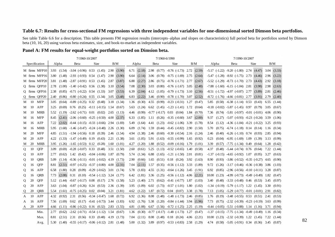
82
Table 6.7: Results for cross-sectional FM regressions with three independent variables for one-dimensional sorted Dimson beta portfolios.
See table Table 6.6 for a description. This table presents FM regression results (intercepts–alphas and slopes on characteristics) full period beta for portfolios sorted by Dimson
beta (10, 16, 20) using various beta estimates, size, and book-to-market as independent variables.
Panel A: FM results for equal-weight portfolios sorted on Dimsion beta.
M firms MFP10 3.93 (1.54) -3.04 (-0.96) 0.53 (1.45) 2.90 (3.90) 6.71 (2.18) 2.98 (0.77) -0.76 (-1.73) 2.72 (2.59) -5.17 (-1.22) -9.20 (-1.80) 2.74 (4.47) 3.04 (3.33)
M firms MFP16 3.80 (1.48) -2.93 (-0.93) 0.54 (1.47) 2.90 (3.90) 6.64 (2.14) 3.06 (0.78) -0.75 (-1.69) 2.75 (2.64) -5.47 (-1.28) -8.92 (-1.75) 2.73 (4.46) 2.96 (3.22)
M firms MFP20 3.81 (1.48) -2.87 (-0.91) 0.53 (1.45) 2.87 (3.87) 6.88 (2.27) 2.86 (0.75) -0.76 (-1.71) 2.77 (2.67) -5.52 (-1.29) -8.73 (-1.70) 2.73 (4.43) 2.92 (3.18)
Q firms QFP10 2.78 (1.00) -1.40 (-0.42) 0.56 (1.38) 3.10 (3.54) 7.08 (2.30) 3.03 (0.80) -0.76 (-1.67) 3.05 (2.48) -7.88 (-1.60) -6.15 (-1.04) 2.81 (3.98) 2.98 (2.63)
Q firms QFP16 2.38 (0.85) -0.71 (-0.22) 0.54 (1.33) 3.07 (3.53) 6.39 (2.04) 4.12 (1.05) -0.79 (-1.73) 3.10 (2.56) -8.51 (-1.72) -4.97 (-0.87) 2.77 (3.89) 2.81 (2.46)
Q firms QFP20 2.40 (0.86) -0.80 (-0.24) 0.55 (1.34) 3.05 (3.48) 6.83 (2.22) 3.46 (0.90) -0.78 (-1.70) 3.07 (2.52) -8.72 (-1.76) -4.66 (-0.81) 2.77 (3.91) 2.79 (2.40)
M 10 MFP 3.05 (0.64) -0.89 (-0.25) 0.32 (0.48) 3.18 (1.34) 1.36 (0.30) 4.55 (0.99) -0.23 (-0.31) 1.27 (0.47) 5.85 (0.58) -6.38 (-1.14) 0.53 (0.43) 6.55 (1.44)
M 10 AFP 3.25 (0.69) 0.76 (0.25) -0.11 (-0.15) 1.54 (0.67) 5.63 (1.24) 6.62 (1.45) -1.23 (-1.41) 1.72 (0.64) -0.18 (-0.02) -5.87 (-1.45) 0.97 (0.79) 3.05 (0.67)
M 10 MRB 5.52 (1.19) -2.62 (-0.71) 0.01 (0.02) 2.65 (1.13) 4.46 (0.99) -0.77 (-0.17) 0.03 (0.04) 1.84 (0.70) 7.36 (0.74) -5.81 (-0.97) -0.01 (-0.01) 4.06 (0.90)
M 16 MFP 8.45 (2.41) -2.06 (-0.60) -0.25 (-0.50) 4.00 (2.37) 6.33 (1.85) 1.11 (0.26) -0.35 (-0.60) 3.67 (2.00) 9.37 (1.27) -5.07 (-0.93) -0.23 (-0.24) 3.59 (1.06)
M 16 AFP 7.22 (2.02) -0.44 (-0.15) -0.33 (-0.66) 2.94 (1.69) 5.49 (1.64) 4.41 (1.23) -0.62 (-1.06) 3.39 (1.78) 8.54 (1.12) -4.36 (-1.04) -0.21 (-0.22) 3.25 (0.93)
M 16 MRB 5.95 (1.68) -1.46 (-0.47) -0.24 (-0.48) 2.26 (1.30) 6.09 (1.74) 1.59 (0.44) -0.45 (-0.82) 2.90 (1.50) 5.70 (0.75) -6.74 (-1.18) 0.14 (0.14) 1.16 (0.34)
M 20 MFP 4.85 (1.51) -1.94 (-0.56) 0.18 (0.39) 2.46 (1.54) 4.94 (1.38) 2.46 (0.60) -0.30 (-0.54) 2.16 (1.24) 2.46 (0.40) -6.26 (-1.10) 0.74 (0.93) 2.85 (0.94)
M 20 AFP 4.22 (1.33) -1.47 (-0.49) 0.19 (0.43) 2.21 (1.38) 3.61 (1.05) 5.91 (1.63) -0.55 (-0.99) 1.65 (0.92) 0.23 (0.04) -6.95 (-1.69) 1.09 (1.39) 3.13 (0.99)
M 20 MRB 3.95 (1.26) -1.65 (-0.53) 0.12 (0.28) 1.60 (1.01) 4.27 (1.20) 1.88 (0.52) -0.09 (-0.16) 1.79 (1.01) 3.39 (0.57) -7.75 (-1.34) 0.49 (0.64) 1.28 (0.42)
Q 10 QFP 3.09 (0.69) -0.28 (-0.07) 0.33 (0.48) 3.51 (1.50) 2.60 (0.61) 5.25 (1.13) -0.52 (-0.65) 1.40 (0.58) 4.37 (0.48) -5.44 (-0.74) 0.76 (0.64) 7.22 (1.44)
Q 10 AFP 2.77 (0.62) 1.42 (0.42) -0.04 (-0.06) 1.87 (0.79) 5.74 (1.34) 6.88 (1.65) -1.21 (-1.50) 2.01 (0.81) -1.37 (-0.15) -4.65 (-0.92) 1.07 (0.95) 3.27 (0.63)
Q 10 QRB 5.09 (1.14) -0.36 (-0.11) -0.01 (-0.02) 4.19 (1.73) 2.90 (0.66) 1.65 (0.51) 0.18 (0.24) 3.92 (1.63) 8.90 (0.93) -3.86 (-0.52) -0.35 (-0.27) 4.65 (0.90)
Q 16 QFP 8.81 (2.51) -0.97 (-0.25) -0.37 (-0.80) 4.00 (2.31) 7.04 (2.11) 1.57 (0.35) -0.56 (-1.12) 3.33 (1.89) 9.72 (1.26) -3.17 (-0.46) -0.36 (-0.38) 3.86 (1.03)
Q 16 AFP 6.58 (1.80) 0.28 (0.09) -0.29 (-0.62) 3.01 (1.74) 5.78 (1.83) 4.55 (1.31) -0.64 (-1.26) 3.45 (1.91) 6.92 (0.85) -2.96 (-0.56) -0.10 (-0.11) 3.28 (0.87)
Q 16 QRB 7.73 (2.08) 0.31 (0.10) -0.54 (-1.12) 3.24 (1.77) 6.42 (1.81) 3.36 (1.25) -0.56 (-1.12) 4.06 (2.21) 10.00 (1.23) -4.99 (-0.73) -0.49 (-0.49) 1.82 (0.47)
Q 20 QFP 5.12 (1.44) -0.67 (-0.17) 0.08 (0.17) 2.76 (1.58) 5.23 (1.40) 2.71 (0.62) -0.41 (-0.77) 1.87 (1.03) 3.40 (0.48) -3.33 (-0.48) 0.46 (0.53) 3.45 (0.97)
Q 20 AFP 3.63 (1.04) -0.87 (-0.26) 0.24 (0.53) 2.36 (1.39) 3.95 (1.09) 6.02 (1.73) -0.57 (-1.01) 1.80 (1.02) -1.34 (-0.19) -5.79 (-1.17) 1.22 (1.45) 3.30 (0.91)
Q 20 QRB 5.54 (1.61) -0.75 (-0.25) 0.02 (0.04) 3.21 (1.81) 4.62 (1.22) 1.87 (0.72) 0.04 (0.07) 3.38 (1.78) 7.13 (1.05) -5.29 (-0.77) -0.01 (-0.01) 2.91 (0.82)
A 10 AFP 4.32 (0.92) 2.31 (0.56) -0.34 (-0.47) 1.68 (0.72) 6.92 (1.36) 8.08 (1.48) -1.48 (-1.73) 2.46 (0.85) 1.76 (0.19) -3.48 (-0.55) 0.53 (0.51) 2.41 (0.53)
A 16 AFP 7.56 (1.69) 0.62 (0.17) -0.41 (-0.73) 3.44 (1.83) 6.92 (1.76) 5.38 (1.20) -0.84 (-1.44) 3.94 (1.96) 7.73 (0.75) -2.32 (-0.39) -0.23 (-0.19) 3.63 (0.99)
A 20 AFP 4.66 (1.11) -0.86 (-0.22) 0.16 (0.32) 2.83 (1.55) 4.81 (1.08) 6.67 (1.56) -0.72 (-1.25) 2.25 (1.19) -0.44 (-0.05) -5.51 (-0.88) 1.14 (1.16) 3.71 (0.94)
Min. 2.77 (0.62) -2.62 (-0.71) -0.54 (-1.12) 1.54 (0.67) 1.36 (0.30) -0.77 (-0.17) -1.48 (-1.73) 1.27 (0.47) -1.37 (-0.15) -7.75 (-1.34) -0.49 (-0.49) 1.16 (0.34)
Max. 8.81 (2.51) 2.31 (0.56) 0.33 (0.48) 4.19 (1.73) 7.04 (2.11) 8.08 (1.48) 0.18 (0.24) 4.06 (2.21) 10.00 (1.23) -2.32 (-0.39) 1.22 (1.45) 7.22 (1.44)
Avg. 5.30 (1.40) -0.55 (-0.17) -0.06 (-0.12) 2.81 (1.48) 5.00 (1.32) 3.89 (0.97) -0.53 (-0.83) 2.58 (1.29) 4.74 (0.58) -5.05 (-0.91) 0.34 (0.36) 3.45 (0.87)
Specification Alpha Beta Size B/M Size B/M Alpha Beta Size B/M
7/1960-10/2007 7/1960-6/1990 7/1990-10/2007
Alpha Beta
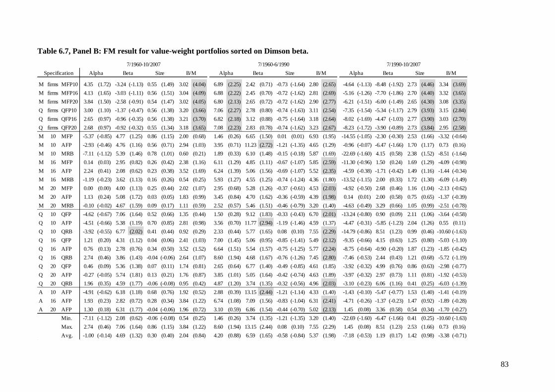
83
Table 6.7, Panel B: FM result for value-weight portfolios sorted on Dimson beta.
M firms MFP10 4.35 (1.72) -3.24 (-1.13) 0.55 (1.49) 3.02 (4.04) 6.89 (2.25) 2.42 (0.71) -0.73 (-1.64) 2.80 (2.65) -4.64 (-1.13) -8.48 (-1.92) 2.73 (4.46) 3.34 (3.69)
M firms MFP16 4.13 (1.65) -3.03 (-1.11) 0.56 (1.51) 3.04 (4.09) 6.88 (2.22) 2.45 (0.70) -0.72 (-1.62) 2.81 (2.69) -5.16 (-1.26) -7.70 (-1.86) 2.70 (4.40) 3.32 (3.65)
M firms MFP20 3.84 (1.50) -2.58 (-0.91) 0.54 (1.47) 3.02 (4.05) 6.80 (2.13) 2.65 (0.72) -0.72 (-1.62) 2.90 (2.77) -6.21 (-1.51) -6.00 (-1.49) 2.65 (4.30) 3.08 (3.35)
Q firms QFP10 3.00 (1.10) -1.37 (-0.47) 0.56 (1.38) 3.20 (3.66) 7.06 (2.27) 2.78 (0.80) -0.74 (-1.63) 3.11 (2.54) -7.35 (-1.54) -5.34 (-1.17) 2.79 (3.93) 3.15 (2.84)
Q firms QFP16 2.65 (0.97) -0.96 (-0.35) 0.56 (1.38) 3.21 (3.70) 6.82 (2.18) 3.12 (0.88) -0.75 (-1.64) 3.18 (2.64) -8.02 (-1.69) -4.47 (-1.03) 2.77 (3.90) 3.03 (2.70)
Q firms QFP20 2.68 (0.97) -0.92 (-0.32) 0.55 (1.34) 3.18 (3.65) 7.08 (2.23) 2.83 (0.78) -0.74 (-1.62) 3.23 (2.67) -8.23 (-1.72) -3.90 (-0.89) 2.73 (3.84) 2.95 (2.58)
M 10 MFP -5.37 (-0.85) 4.77 (1.25) 0.86 (1.15) 2.00 (0.68) 1.46 (0.26) 6.65 (1.50) 0.01 (0.01) 6.93 (1.95) -14.55 (-1.05) -2.30 (-0.30) 2.53 (1.66) -3.32 (-0.64)
M 10 AFP -2.93 (-0.46) 4.76 (1.16) 0.56 (0.71) 2.94 (1.03) 3.95 (0.71) 11.23 (2.72) -1.21 (-1.35) 4.65 (1.29) -0.96 (-0.07) -6.47 (-1.66) 1.70 (1.17) 0.73 (0.16)
M 10 MRB -7.11 (-1.12) 5.39 (1.46) 0.78 (1.01) 0.60 (0.21) 1.89 (0.33) 6.10 (1.48) -0.15 (-0.18) 5.87 (1.69) -22.69 (-1.60) 4.15 (0.58) 2.38 (1.52) -8.51 (-1.64)
M 16 MFP 0.14 (0.03) 2.95 (0.82) 0.26 (0.42) 2.38 (1.16) 6.11 (1.29) 4.85 (1.11) -0.67 (-1.07) 5.85 (2.59) -11.30 (-0.96) 1.50 (0.24) 1.69 (1.29) -4.09 (-0.98)
M 16 AFP 2.24 (0.41) 2.08 (0.62) 0.23 (0.38) 3.52 (1.69) 6.24 (1.39) 5.06 (1.56) -0.69 (-1.07) 5.52 (2.35) -4.59 (-0.38) -1.71 (-0.42) 1.49 (1.16) -1.44 (-0.34)
M 16 MRB -1.19 (-0.23) 3.62 (1.13) 0.16 (0.26) 0.54 (0.25) 5.93 (1.27) 4.55 (1.25) -0.74 (-1.24) 4.36 (1.80) -13.52 (-1.15) 2.00 (0.33) 1.72 (1.30) -6.09 (-1.49)
M 20 MFP 0.00 (0.00) 4.00 (1.13) 0.25 (0.44) 2.02 (1.07) 2.95 (0.68) 5.28 (1.26) -0.37 (-0.61) 4.53 (2.03) -4.92 (-0.50) 2.68 (0.46) 1.16 (1.04) -2.13 (-0.62)
M 20 AFP 1.13 (0.24) 5.08 (1.72) 0.03 (0.05) 1.83 (0.99) 3.45 (0.84) 4.70 (1.62) -0.36 (-0.59) 4.39 (1.98) 0.14 (0.01) 2.00 (0.58) 0.75 (0.65) -1.37 (-0.39)
M 20 MRB -0.10 (-0.02) 4.67 (1.59) 0.09 (0.17) 1.11 (0.59) 2.52 (0.57) 5.46 (1.51) -0.46 (-0.79) 3.20 (1.40) -4.63 (-0.49) 3.29 (0.66) 1.05 (0.99) -2.51 (-0.78)
Q 10 QFP -4.62 (-0.67) 7.06 (1.64) 0.52 (0.66) 1.35 (0.44) 1.50 (0.28) 9.12 (1.83) -0.33 (-0.43) 6.70 (2.01) -13.24 (-0.80) 0.90 (0.09) 2.11 (1.06) -3.64 (-0.58)
Q 10 AFP -4.51 (-0.66) 5.38 (1.19) 0.70 (0.85) 2.81 (0.98) 3.56 (0.70) 11.77 (2.94) -1.19 (-1.46) 4.59 (1.37) -4.47 (-0.31) -5.85 (-1.23) 2.04 (1.26) 0.55 (0.11)
Q 10 QRB -3.92 (-0.55) 6.77 (2.02) 0.41 (0.44) 0.92 (0.29) 2.33 (0.44) 5.77 (1.65) 0.08 (0.10) 7.55 (2.29) -14.79 (-0.86) 8.51 (1.23) 0.99 (0.46) -10.60 (-1.63)
Q 16 QFP 1.21 (0.20) 4.31 (1.12) 0.04 (0.06) 2.41 (1.03) 7.00 (1.45) 5.06 (0.95) -0.85 (-1.41) 5.49 (2.12) -9.35 (-0.66) 4.15 (0.63) 1.25 (0.80) -5.03 (-1.10)
Q 16 AFP 0.76 (0.13) 2.78 (0.76) 0.34 (0.50) 3.52 (1.52) 6.64 (1.51) 5.54 (1.57) -0.75 (-1.25) 5.77 (2.24) -8.75 (-0.64) -0.90 (-0.20) 1.87 (1.23) -1.85 (-0.42)
Q 16 QRB 2.74 (0.46) 3.86 (1.43) -0.04 (-0.06) 2.64 (1.07) 8.60 (1.94) 4.68 (1.67) -0.76 (-1.26) 7.45 (2.80) -7.46 (-0.53) 2.44 (0.43) 1.21 (0.68) -5.72 (-1.19)
Q 20 QFP 0.46 (0.09) 5.36 (1.38) 0.07 (0.11) 1.74 (0.81) 2.65 (0.64) 6.77 (1.40) -0.49 (-0.85) 4.61 (1.85) -3.92 (-0.32) 4.99 (0.76) 0.86 (0.63) -2.98 (-0.77)
Q 20 AFP -0.27 (-0.05) 5.74 (1.81) 0.13 (0.21) 1.76 (0.87) 3.85 (1.01) 5.05 (1.64) -0.42 (-0.74) 4.63 (1.89) -3.97 (-0.32) 2.97 (0.73) 1.11 (0.81) -1.92 (-0.53)
Q 20 QRB 1.96 (0.35) 4.59 (1.77) -0.06 (-0.08) 0.95 (0.42) 4.87 (1.20) 3.74 (1.35) -0.32 (-0.56) 4.96 (2.03) -3.10 (-0.23) 6.06 (1.16) 0.41 (0.25) -6.03 (-1.39)
A 10 AFP -4.91 (-0.62) 6.18 (1.18) 0.68 (0.76) 1.92 (0.52) 2.88 (0.39) 13.15 (2.44) -1.21 (-1.14) 4.33 (1.40) -1.43 (-0.10) -5.47 (-0.77) 1.53 (1.40) -1.41 (-0.19)
A 16 AFP 1.93 (0.23) 2.82 (0.72) 0.28 (0.34) 3.84 (1.22) 6.74 (1.08) 7.09 (1.56) -0.83 (-1.04) 6.31 (2.41) -4.71 (-0.26) -1.37 (-0.23) 1.47 (0.92) -1.89 (-0.28)
A 20 AFP 1.30 (0.18) 6.31 (1.77) -0.04 (-0.06) 1.96 (0.72) 3.10 (0.59) 6.86 (1.54) -0.44 (-0.70) 5.02 (2.13) 1.45 (0.08) 3.36 (0.58) 0.54 (0.34) -1.70 (-0.27)
Min. -7.11 (-1.12) 2.08 (0.62) -0.06 (-0.08) 0.54 (0.25) 1.46 (0.26) 3.74 (1.35) -1.21 (-1.35) 3.20 (1.40) -22.69 (-1.60) -6.47 (-1.66) 0.41 (0.25) -10.60 (-1.63)
Max. 2.74 (0.46) 7.06 (1.64) 0.86 (1.15) 3.84 (1.22) 8.60 (1.94) 13.15 (2.44) 0.08 (0.10) 7.55 (2.29) 1.45 (0.08) 8.51 (1.23) 2.53 (1.66) 0.73 (0.16)
Avg. -1.00 (-0.14) 4.69 (1.32) 0.30 (0.40) 2.04 (0.84) 4.20 (0.88) 6.59 (1.65) -0.58 (-0.84) 5.37 (1.98) -7.18 (-0.53) 1.19 (0.17) 1.42 (0.98) -3.38 (-0.71)
Specification Alpha Beta Size B/M Alpha Beta Size B/M
7/1960-10/2007 7/1960-6/1990 7/1990-10/2007
Alpha Beta Size B/M
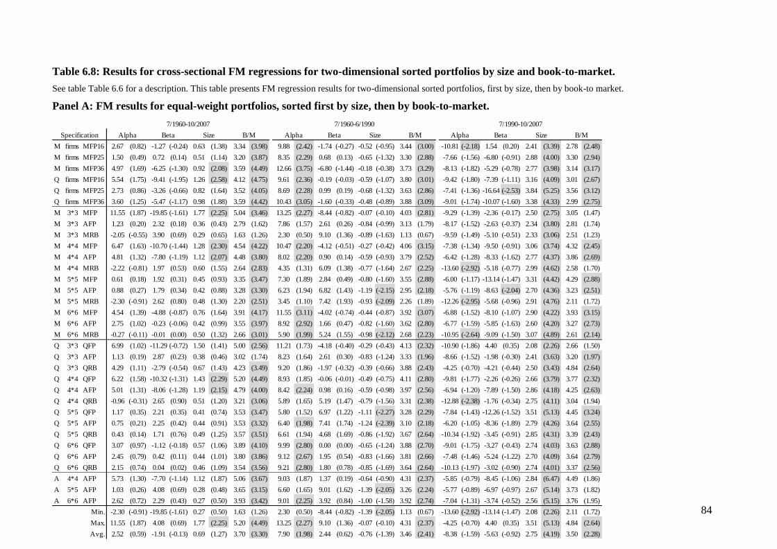
84
Table 6.8: Results for cross-sectional FM regressions for two-dimensional sorted portfolios by size and book-to-market.
See table Table 6.6 for a description. This table presents FM regression results for two-dimensional sorted portfolios, first by size, then by book-to market.
Panel A: FM results for equal-weight portfolios, sorted first by size, then by book-to-market.
M firms MFP16 2.67 (0.82) -1.27 (-0.24) 0.63 (1.38) 3.34 (3.98) 9.88 (2.42) -1.74 (-0.27) -0.52 (-0.95) 3.44 (3.00) -10.81 (-2.18) 1.54 (0.20) 2.41 (3.39) 2.78 (2.48)
M firms MFP25 1.50 (0.49) 0.72 (0.14) 0.51 (1.14) 3.20 (3.87) 8.35 (2.29) 0.68 (0.13) -0.65 (-1.32) 3.30 (2.88) -7.66 (-1.56) -6.80 (-0.91) 2.88 (4.00) 3.30 (2.94)
M firms MFP36 4.97 (1.69) -6.25 (-1.30) 0.92 (2.08) 3.59 (4.49) 12.66 (3.75) -6.80 (-1.44) -0.18 (-0.38) 3.73 (3.29) -8.13 (-1.82) -5.29 (-0.78) 2.77 (3.98) 3.14 (3.17)
Q firms MFP16 5.54 (1.75) -9.41 (-1.95) 1.26 (2.58) 4.12 (4.75) 9.61 (2.36) -0.19 (-0.03) -0.59 (-1.07) 3.80 (3.01) -9.42 (-1.80) -7.39 (-1.11) 3.16 (4.09) 3.01 (2.67)
Q firms MFP25 2.73 (0.86) -3.26 (-0.66) 0.82 (1.64) 3.52 (4.05) 8.69 (2.28) 0.99 (0.19) -0.68 (-1.32) 3.63 (2.86) -7.41 (-1.36) -16.64 (-2.53) 3.84 (5.25) 3.56 (3.12)
Q firms MFP36 3.60 (1.25) -5.47 (-1.17) 0.98 (1.88) 3.59 (4.42) 10.43 (3.05) -1.60 (-0.33) -0.48 (-0.89) 3.88 (3.09) -9.01 (-1.74) -10.07 (-1.60) 3.38 (4.33) 2.99 (2.75)
M 3*3 MFP 11.55 (1.87) -19.85 (-1.61) 1.77 (2.25) 5.04 (3.46) 13.25 (2.27) -8.44 (-0.82) -0.07 (-0.10) 4.03 (2.81) -9.29 (-1.39) -2.36 (-0.17) 2.50 (2.75) 3.05 (1.47)
M 3*3 AFP 1.23 (0.20) 2.32 (0.18) 0.36 (0.43) 2.79 (1.62) 7.86 (1.57) 2.61 (0.26) -0.84 (-0.99) 3.13 (1.79) -8.17 (-1.52) -2.63 (-0.37) 2.34 (3.80) 2.81 (1.74)
M 3*3 MRB -2.05 (-0.55) 3.90 (0.69) 0.29 (0.65) 1.63 (1.26) 2.30 (0.50) 9.10 (1.36) -0.89 (-1.63) 1.13 (0.67) -9.59 (-1.49) -5.10 (-0.51) 2.33 (3.06) 2.51 (1.23)
M 4*4 MFP 6.47 (1.63) -10.70 (-1.44) 1.28 (2.30) 4.54 (4.22) 10.47 (2.20) -4.12 (-0.51) -0.27 (-0.42) 4.06 (3.15) -7.38 (-1.34) -9.50 (-0.91) 3.06 (3.74) 4.32 (2.45)
M 4*4 AFP 4.81 (1.32) -7.80 (-1.19) 1.12 (2.07) 4.48 (3.80) 8.02 (2.20) 0.90 (0.14) -0.59 (-0.93) 3.79 (2.52) -6.42 (-1.28) -8.33 (-1.62) 2.77 (4.37) 3.86 (2.69)
M 4*4 MRB -2.22 (-0.81) 1.97 (0.53) 0.60 (1.55) 2.64 (2.83) 4.35 (1.31) 6.09 (1.38) -0.77 (-1.64) 2.67 (2.25) -13.60 (-2.92) -5.18 (-0.77) 2.99 (4.62) 2.58 (1.70)
M 5*5 MFP 0.61 (0.18) 1.92 (0.31) 0.45 (0.93) 3.35 (3.47) 7.30 (1.89) 2.84 (0.49) -0.80 (-1.60) 3.55 (2.88) -6.00 (-1.17) -13.14 (-1.47) 3.31 (4.42) 4.29 (2.88)
M 5*5 AFP 0.88 (0.27) 1.79 (0.34) 0.42 (0.88) 3.28 (3.30) 6.23 (1.94) 6.82 (1.43) -1.19 (-2.15) 2.95 (2.18) -5.76 (-1.19) -8.63 (-2.04) 2.70 (4.36) 3.23 (2.51)
M 5*5 MRB -2.30 (-0.91) 2.62 (0.80) 0.48 (1.30) 2.20 (2.51) 3.45 (1.10) 7.42 (1.93) -0.93 (-2.09) 2.26 (1.89) -12.26 (-2.95) -5.68 (-0.96) 2.91 (4.76) 2.11 (1.72)
M 6*6 MFP 4.54 (1.39) -4.88 (-0.87) 0.76 (1.64) 3.91 (4.17) 11.55 (3.11) -4.02 (-0.74) -0.44 (-0.87) 3.92 (3.07) -6.88 (-1.52) -8.10 (-1.07) 2.90 (4.22) 3.93 (3.15)
M 6*6 AFP 2.75 (1.02) -0.23 (-0.06) 0.42 (0.99) 3.55 (3.97) 8.92 (2.92) 1.66 (0.47) -0.82 (-1.60) 3.62 (2.80) -6.77 (-1.59) -5.85 (-1.63) 2.60 (4.20) 3.27 (2.73)
M 6*6 MRB -0.27 (-0.11) -0.01 (0.00) 0.50 (1.32) 2.66 (3.01) 5.90 (1.99) 5.24 (1.55) -0.98 (-2.12) 2.68 (2.23) -10.95 (-2.64) -9.09 (-1.50) 3.07 (4.89) 2.61 (2.14)
Q 3*3 QFP 6.99 (1.02) -11.29 (-0.72) 1.50 (1.41) 5.00 (2.56) 11.21 (1.73) -4.18 (-0.40) -0.29 (-0.43) 4.13 (2.32) -10.90 (-1.86) 4.40 (0.35) 2.08 (2.26) 2.66 (1.50)
Q 3*3 AFP 1.13 (0.19) 2.87 (0.23) 0.38 (0.46) 3.02 (1.74) 8.23 (1.64) 2.61 (0.30) -0.83 (-1.24) 3.33 (1.96) -8.66 (-1.52) -1.98 (-0.30) 2.41 (3.63) 3.20 (1.97)
Q 3*3 QRB 4.29 (1.11) -2.79 (-0.54) 0.67 (1.43) 4.23 (3.49) 9.20 (1.86) -1.97 (-0.32) -0.39 (-0.66) 3.88 (2.43) -4.25 (-0.70) -4.21 (-0.44) 2.50 (3.43) 4.84 (2.64)
Q 4*4 QFP 6.22 (1.58) -10.32 (-1.31) 1.43 (2.29) 5.20 (4.49) 8.93 (1.85) -0.06 (-0.01) -0.49 (-0.75) 4.11 (2.80) -9.81 (-1.77) -2.26 (-0.26) 2.66 (3.79) 3.77 (2.32)
Q 4*4 AFP 5.01 (1.31) -8.06 (-1.28) 1.19 (2.15) 4.79 (4.00) 8.42 (2.24) 0.98 (0.16) -0.59 (-0.98) 3.97 (2.56) -6.94 (-1.20) -7.89 (-1.50) 2.86 (4.18) 4.25 (2.63)
Q 4*4 QRB -0.96 (-0.31) 2.65 (0.90) 0.51 (1.20) 3.21 (3.06) 5.89 (1.65) 5.19 (1.47) -0.79 (-1.56) 3.31 (2.38) -12.88 (-2.38) -1.76 (-0.34) 2.75 (4.11) 3.04 (1.94)
Q 5*5 QFP 1.17 (0.35) 2.21 (0.35) 0.41 (0.74) 3.53 (3.47) 5.80 (1.52) 6.97 (1.22) -1.11 (-2.27) 3.28 (2.29) -7.84 (-1.43) -12.26 (-1.52) 3.51 (5.13) 4.45 (3.24)
Q 5*5 AFP 0.75 (0.21) 2.25 (0.42) 0.44 (0.91) 3.53 (3.32) 6.40 (1.98) 7.41 (1.74) -1.24 (-2.39) 3.10 (2.18) -6.20 (-1.05) -8.36 (-1.89) 2.79 (4.26) 3.64 (2.55)
Q 5*5 QRB 0.43 (0.14) 1.71 (0.76) 0.49 (1.25) 3.57 (3.51) 6.61 (1.94) 4.68 (1.69) -0.86 (-1.92) 3.67 (2.64) -10.34 (-1.92) -3.45 (-0.91) 2.85 (4.31) 3.39 (2.43)
Q 6*6 QFP 3.07 (0.97) -1.12 (-0.18) 0.57 (1.06) 3.89 (4.10) 9.99 (2.80) 0.00 (0.00) -0.65 (-1.24) 3.88 (2.70) -9.01 (-1.75) -3.27 (-0.43) 2.74 (4.03) 3.63 (2.88)
Q 6*6 AFP 2.45 (0.79) 0.42 (0.11) 0.44 (1.01) 3.80 (3.86) 9.12 (2.67) 1.95 (0.54) -0.83 (-1.66) 3.81 (2.66) -7.48 (-1.46) -5.24 (-1.22) 2.70 (4.09) 3.64 (2.79)
Q 6*6 QRB 2.15 (0.74) 0.04 (0.02) 0.46 (1.09) 3.54 (3.56) 9.21 (2.80) 1.80 (0.78) -0.85 (-1.69) 3.64 (2.64) -10.13 (-1.97) -3.02 (-0.90) 2.74 (4.01) 3.37 (2.56)
A 4*4 AFP 5.73 (1.30) -7.70 (-1.14) 1.12 (1.87) 5.06 (3.67) 9.03 (1.87) 1.37 (0.19) -0.64 (-0.90) 4.31 (2.37) -5.85 (-0.79) -8.45 (-1.06) 2.84 (6.47) 4.49 (1.86)
A 5*5 AFP 1.03 (0.26) 4.08 (0.69) 0.28 (0.48) 3.65 (3.15) 6.60 (1.65) 9.01 (1.62) -1.39 (-2.05) 3.26 (2.24) -5.77 (-0.89) -6.97 (-0.97) 2.67 (5.14) 3.73 (1.82)
A 6*6 AFP 2.62 (0.72) 2.29 (0.43) 0.27 (0.50) 3.93 (3.42) 9.01 (2.25) 3.92 (0.84) -1.00 (-1.58) 3.92 (2.74) -7.04 (-1.31) -3.74 (-0.52) 2.56 (5.15) 3.76 (1.95)
-2.30 (-0.91) -19.85 (-1.61) 0.27 (0.50) 1.63 (1.26) 2.30 (0.50) -8.44 (-0.82) -1.39 (-2.05) 1.13 (0.67) -13.60 (-2.92) -13.14 (-1.47) 2.08 (2.26) 2.11 (1.72)
11.55 (1.87) 4.08 (0.69) 1.77 (2.25) 5.20 (4.49) 13.25 (2.27) 9.10 (1.36) -0.07 (-0.10) 4.31 (2.37) -4.25 (-0.70) 4.40 (0.35) 3.51 (5.13) 4.84 (2.64)
2.52 (0.59) -1.91 (-0.13) 0.69 (1.27) 3.70 (3.30) 7.90 (1.98) 2.44 (0.62) -0.76 (-1.39) 3.46 (2.41) -8.38 (-1.59) -5.63 (-0.92) 2.75 (4.19) 3.50 (2.28)
Specification
Avg.
Min.
Max.
Beta Size B/M Alpha Beta Size B/MAlpha Beta Size B/M Alpha
7/1960-10/2007 7/1960-6/1990 7/1990-10/2007
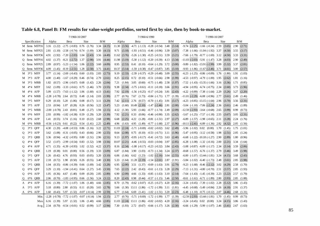
85
Table 6.8, Panel B: FM results for value-weight portfolios, sorted first by size, then by book-to-market.
M firms MFP16 3.16 (1.22) -2.75 (-0.83) 0.76 (1.76) 3.34 (4.15) 11.30 (3.56) -4.71 (-1.13) -0.28 (-0.54) 3.48 (3.14) -9.74 (-2.25) -1.66 (-0.34) 2.59 (3.65) 2.90 (2.71)
M firms MFP25 2.81 (1.10) -2.58 (-0.74) 0.74 (1.69) 3.30 (4.13) 9.71 (3.18) -1.93 (-0.51) -0.46 (-0.96) 3.39 (3.07) -7.38 (-1.66) -11.04 (-1.92) 3.37 (4.50) 3.55 (3.17)
M firms MFP36 4.91 (1.92) -7.20 (-2.03) 1.04 (2.43) 3.56 (4.49) 11.62 (3.76) -5.26 (-1.30) -0.25 (-0.51) 3.59 (3.21) -7.66 (-1.79) -8.77 (-1.69) 3.12 (4.50) 3.33 (3.31)
Q firms MFP16 4.02 (1.37) -8.21 (-2.72) 1.37 (2.98) 3.91 (4.44) 11.98 (3.19) -5.30 (-1.12) -0.20 (-0.39) 4.13 (3.34) -11.03 (-2.03) -5.91 (-1.47) 3.28 (4.03) 2.90 (2.49)
Q firms MFP25 2.89 (0.97) -5.23 (-1.54) 1.06 (2.22) 3.60 (4.09) 8.95 (2.53) 0.41 (0.10) -0.64 (-1.29) 3.72 (3.00) -9.89 (-1.82) -13.91 (-2.99) 3.99 (5.32) 3.37 (2.81)
Q firms MFP36 4.09 (1.45) -8.19 (-2.51) 1.28 (2.58) 3.75 (4.41) 10.37 (3.14) -1.59 (-0.38) -0.47 (-0.87) 3.85 (3.10) -9.93 (-1.86) -11.67 (-2.46) 3.71 (4.61) 3.00 (2.57)
M 3*3 MFP 3.77 (1.14) -2.69 (-0.43) 0.60 (1.03) 2.83 (2.73) 9.19 (2.33) -2.39 (-0.37) -0.29 (-0.48) 3.09 (2.55) -6.23 (-1.25) -0.86 (-0.09) 1.76 (1.80) 1.91 (1.03)
M 3*3 AFP 4.00 (1.40) -1.67 (-0.29) 0.46 (0.74) 2.79 (2.61) 8.25 (2.15) 0.72 (0.10) -0.51 (-0.66) 2.98 (1.99) -4.53 (-0.97) -4.79 (-1.00) 1.95 (2.62) 1.81 (1.16)
M 3*3 MRB 1.82 (0.57) -2.96 (-0.67) 0.68 (1.42) 2.26 (2.04) 7.21 (1.84) 3.05 (0.60) -0.75 (-1.48) 2.58 (1.97) -7.52 (-1.43) -13.35 (-1.66) 3.16 (3.36) 1.71 (0.85)
M 4*4 MFP 3.62 (1.09) -3.33 (-0.61) 0.75 (1.46) 3.70 (3.55) 9.38 (2.34) -3.75 (-0.61) -0.11 (-0.18) 3.66 (2.91) -4.94 (-0.95) -6.74 (-0.75) 2.34 (2.60) 3.73 (1.96)
M 4*4 AFP 5.09 (1.57) -7.63 (-1.12) 1.06 (1.60) 4.13 (3.41) 7.92 (2.19) -1.56 (-0.25) -0.17 (-0.24) 3.81 (2.43) -4.22 (-0.89) -7.38 (-1.64) 2.29 (3.26) 3.27 (2.20)
M 4*4 MRB -2.28 (-0.78) 2.64 (0.72) 0.48 (1.14) 2.03 (1.99) 2.77 (0.76) 7.67 (1.73) -0.84 (-1.71) 1.77 (1.39) -11.01 (-2.29) -6.08 (-0.96) 2.77 (3.61) 2.49 (1.46)
M 5*5 MFP 0.29 (0.10) 5.20 (1.06) 0.08 (0.17) 3.11 (3.29) 7.42 (2.11) 2.76 (0.57) -0.70 (-1.45) 3.91 (3.17) -4.23 (-0.85) -13.15 (-1.64) 2.96 (3.70) 3.56 (2.31)
M 5*5 AFP 2.53 (0.94) 1.07 (0.28) 0.26 (0.56) 3.22 (3.47) 5.23 (1.60) 10.49 (2.10) -1.47 (-2.46) 2.81 (2.00) -5.04 (-1.10) -7.06 (-2.24) 2.36 (3.61) 2.46 (1.89)
M 5*5 MRB -2.00 (-0.78) 2.43 (0.81) 0.48 (1.27) 1.94 (2.15) 4.12 (1.30) 5.93 (1.66) -0.77 (-1.74) 2.49 (2.09) -12.59 (-2.93) -3.64 (-0.68) 2.65 (3.99) 0.99 (0.73)
M 6*6 MFP 2.93 (0.99) -1.82 (-0.38) 0.59 (1.29) 3.20 (3.39) 7.92 (2.21) 0.33 (0.06) -0.46 (-0.90) 3.35 (2.62) -5.67 (-1.25) -7.57 (-1.18) 2.55 (3.67) 3.05 (2.31)
M 6*6 AFP 1.41 (0.55) 3.74 (1.16) 0.10 (0.22) 2.68 (2.98) 6.68 (2.25) 4.22 (1.28) -0.81 (-1.51) 2.97 (2.27) -6.89 (-1.57) -1.98 (-0.65) 2.11 (3.28) 2.24 (1.76)
M 6*6 MRB -0.56 (-0.23) 0.61 (0.22) 0.54 (1.41) 2.25 (2.49) 4.96 (1.63) 4.95 (1.49) -0.77 (-1.68) 2.37 (1.96) -10.11 (-2.41) -6.89 (-1.36) 2.82 (4.32) 2.05 (1.56)
Q 3*3 QFP 4.30 (1.20) -4.08 (-0.53) 0.86 (1.16) 3.22 (2.71) 11.03 (2.24) -5.71 (-0.69) -0.02 (-0.02) 3.62 (2.49) -5.96 (-1.02) 0.02 (0.00) 1.70 (1.45) 1.75 (1.01)
Q 3*3 AFP 3.62 (1.08) -0.31 (-0.05) 0.43 (0.66) 2.90 (2.55) 8.64 (2.08) 0.75 (0.10) -0.53 (-0.71) 3.11 (1.96) -5.47 (-0.95) -3.12 (-0.58) 1.98 (2.51) 2.05 (1.24)
Q 3*3 QRB 3.36 (0.94) -4.32 (-0.95) 0.80 (1.51) 2.96 (2.51) 9.13 (1.97) -0.95 (-0.17) -0.41 (-0.72) 3.63 (2.40) -6.68 (-1.22) -10.18 (-1.27) 2.90 (2.89) 1.80 (0.96)
Q 4*4 QFP 3.52 (1.07) -2.99 (-0.54) 0.83 (1.52) 3.98 (3.56) 10.07 (2.21) -4.46 (-0.55) -0.03 (-0.04) 3.97 (2.85) -6.28 (-1.08) -1.32 (-0.16) 2.00 (2.21) 3.34 (1.64)
Q 4*4 AFP 4.71 (1.35) -6.39 (-0.93) 1.02 (1.52) 4.22 (3.37) 8.16 (2.34) -1.08 (-0.17) -0.23 (-0.32) 3.84 (2.43) -5.08 (-0.87) -6.09 (-1.17) 2.34 (3.14) 3.59 (2.06)
Q 4*4 QRB 1.19 (0.38) 0.01 (0.00) 0.56 (1.19) 3.33 (3.09) 6.87 (1.84) 3.90 (1.03) -0.73 (-1.34) 3.24 (2.37) -8.68 (-1.57) -6.76 (-1.37) 2.79 (3.46) 3.49 (1.98)
Q 5*5 QFP 1.26 (0.42) 4.76 (0.93) 0.03 (0.05) 3.20 (3.10) 6.06 (1.66) 6.62 (1.23) -1.02 (-2.16) 3.64 (2.55) -6.00 (-1.07) -13.44 (-1.81) 3.24 (4.15) 3.68 (2.43)
Q 5*5 AFP 2.18 (0.72) 1.98 (0.50) 0.26 (0.55) 3.40 (3.30) 5.33 (1.64) 11.28 (2.19) -1.54 (-2.61) 2.87 (1.91) -5.84 (-1.02) -6.40 (-1.73) 2.48 (3.61) 2.85 (1.98)
Q 5*5 QRB 1.04 (0.35) -0.86 (-0.39) 0.66 (1.69) 3.42 (3.28) 6.95 (2.00) 3.51 (1.37) -0.69 (-1.63) 3.91 (2.79) -9.23 (-1.68) -8.46 (-2.12) 3.02 (4.29) 2.58 (1.70)
Q 6*6 QFP 3.29 (1.10) -1.94 (-0.41) 0.64 (1.27) 3.45 (3.50) 7.65 (2.22) 2.42 (0.43) -0.61 (-1.13) 3.28 (2.29) -7.13 (-1.31) -4.80 (-0.70) 2.51 (3.57) 2.85 (1.93)
Q 6*6 AFP 1.05 (0.36) 4.67 (1.40) 0.09 (0.20) 2.85 (2.89) 6.90 (2.09) 4.66 (1.33) -0.85 (-1.63) 3.10 (2.14) -7.64 (-1.43) -1.45 (-0.39) 2.23 (3.22) 2.57 (1.79)
Q 6*6 QRB 2.06 (0.70) -1.83 (-0.95) 0.66 (1.56) 3.24 (3.12) 8.20 (2.43) 0.98 (0.44) -0.57 (-1.15) 3.46 (2.50) -8.61 (-1.61) -6.71 (-1.89) 2.80 (3.93) 2.85 (1.88)
A 4*4 AFP 6.16 (1.39) -7.72 (-1.07) 1.06 (1.40) 4.66 (2.85) 8.70 (1.79) -0.62 (-0.07) -0.25 (-0.27) 4.20 (2.16) -3.24 (-0.45) -7.39 (-1.02) 2.28 (5.12) 3.86 (1.43)
A 5*5 AFP 3.18 (0.80) 2.80 (0.55) 0.11 (0.20) 3.65 (2.78) 5.66 (1.30) 13.11 (1.86) -1.72 (-1.99) 3.11 (1.81) -4.45 (-0.68) -5.49 (-0.84) 2.26 (4.18) 2.91 (1.37)
A 6*6 AFP 1.60 (0.43) 5.97 (1.32) -0.07 (-0.14) 2.99 (2.59) 6.77 (1.64) 6.69 (1.41) -1.02 (-1.51) 3.20 (2.23) -6.48 (-1.10) -0.75 (-0.12) 2.07 (4.46) 2.68 (1.31)
-2.28 (-0.78) -7.72 (-1.07) -0.07 (-0.14) 1.94 (2.15) 2.77 (0.76) -5.71 (-0.69) -1.72 (-1.99) 1.77 (1.39) -12.59 (-2.93) -13.44 (-1.81) 1.70 (1.45) 0.99 (0.73)
6.16 (1.39) 5.97 (1.32) 1.06 (1.40) 4.66 (2.85) 11.03 (2.24) 13.11 (1.86) -0.02 (-0.02) 4.20 (2.16) -3.24 (-0.45) 0.02 (0.00) 3.24 (4.15) 3.86 (1.43)
2.34 (0.70) -0.54 (-0.01) 0.52 (0.99) 3.17 (2.94) 7.30 (1.93) 2.72 (0.67) -0.66 (-1.17) 3.26 (2.30) -6.66 (-1.29) -5.99 (-1.07) 2.46 (3.41) 2.67 (1.63)
7/1960-10/2007 7/1960-6/1990 7/1990-10/2007
Min.
Max.
Avg.
Specification B/MSize B/M Alpha Beta SizeBetaAlpha Beta Size B/M Alpha

86
References
Affleck-Graves, J. / McDonald, B. (1989): Nonnormalities and Tests of Asset Pricing
Theories. The Journal of Finance 44(4), 889-908.
Amel-Zadeh, A. (2011): The Return of the Size Anomaly: Evidence from the German Stock
Market. European Financial Management 17(1), 145-182.
Ang, A. / Chen, J. (2007): CAPM over the long run: 1926-2001. Journal of Empirical
Finance 14(1), 1-40.
Ang, A./ Liu, J. / Schwarz, K. (2010): Using individual stocks or portfolios in tests of factor
models. Working Paper .
Artmann, S./ Finter, P. / Kempf, A. (2010): Determinants of Expected Stock Returns: Large
Sample Evidence from the German Market. Working Paper (CFR) .
Artmann, S./ Finter, P./ Kempf, A./ Koch, S. / Theissen, E. (2012): The Cross-Section of
German Stock Returns: New Data and New Evidence. Schmalenbach Business Review
64, 20-43.
Avramov, D. / Chordia, T. (2006): Asset pricing models and financial market anomalies.
Review of Financial Studies 19(3), 1001.
Baesel, J. (1974): On the assessment of risk: some further considerations. The Journal of
Finance 29(5), 1491-1494.
Bessler, W. / Thies, S. (2007): The long-run performance of initial public offerings in
Germany. Managerial Finance 33(6), 420-441.
Black, F. (1993): Return and beta. Journal of Portfolio Management 20(Fall), 8-18.
Black, F./ Jensen, M. C. / Scholes, M. (1972): The Capital Asset Pricing Model: Some
Empirical TestsStudies in the Theory of Capital Markets Jensen, M.C. (Hrsg.),, Praeger
Publishers, New York, 79-121.
Blume, M. E. (1971): On the Assessment of Risk. The Journal of Finance 26(1), pp. 1-10.
Blume, M. E. / Friend, I. (1973): A New Look at the Capital Asset Pricing Model. The
Journal of Finance 28(1), 19-33.
Brennan, M. J. (1970): Taxes, Market Valuation and Corporate Financial Policy. National Tax
Journal 23(4), 417-427.
Brennan, M. J./ Chordia, T. / Subrahmanyam, A. (1998): Alternative factor specifications,
security characteristics, and the cross-section of expected stock returns. Journal of
Financial Economics 49(3), 345-373.
Brückner, R. / Stehle, R. (2011): Der Geregelte Markt Frankfurt: Ein ökonomischer Nachruf.
Working Paper .
Bulkley, G. / Nawosah, V. (2009): Can the Cross-Sectional Variation in Expected Stock
Returns Explain Momentum?. Journal of Financial and Quantitative Analysis 44(04),
777-794.
Bunke, O./ Sommerfeld, V. / Stehle, R. (1999): Semiparametric modelling of the cross-
section of expected returns in the German stock market. Working Paper, Humboldt-
University .
Campbell, J. / Vuolteenaho, T. (2004): Bad Beta, Good Beta. American Economic Review ,
1249-1275.
Campbell, J. Y./ Lo, A. W. / MacKinlay, A. C. (1997): The Econometrics of Financial
Markets. Princeton University Press, Princeton, NJ.

87
Chan, L. K./ Jegadeesh, N. / Lakonishok, J. (1995): Evaluating the performance of value
versus glamour stocks The impact of selection bias. Journal of Financial Economics
38(3), 269-296.
Chan, L. K. C./ Hamao, Y. / Lakonishok, J. (1991): Fundamentals and Stock Returns in
Japan. The Journal of Finance 46(5), pp. 1739-1764.
Chou, R./ Huang, M./ Lin, J. / Hsu, J. (2009): The Consistency of Size Effect: Time Periods,
Regression Methods, and Database Selection2009 Ninth International Conference on
Hybrid Intelligent Systems, IEEE, 84-88.
Cochrane, J. H. (2005): Asset Pricing. Princeton University Press, Princeton and Oxford.
Daniel, K. / Titman, S. (1997): Evidence on the characteristics of cross sectional variation in
stock returns. Journal of Finance 52(1), 1-33.
Davis, J./ Fama, E. / French, K. (2000): Characteristics, covariances, and average returns:
1929 to 1997. The Journal of Finance 55(1), 389-406.
Davis, J. L. (1994): The Cross-Section of Realized Stock Returns: The Pre-COMPUSTAT
Evidence. The Journal of Finance 49(5), pp. 1579-1593.
DeAngelo, H. / DeAngelo, L. (1985): Managerial ownership of voting rights: A study of
public corporations with dual classes of common stock. Journal of Financial Economics
14(1), 33-69.
Dijk, M. A. v. (2011): Is size dead? A review of the size effect in equity returns. Journal of
Banking & Finance In Press, Corrected Proof, - .
Dimson, E. (1979): Risk Measurement when Shares are Subject to infrequent trading. Journal
of Financial Economics 7(2), 197-226.
Eisenbeiss, M./ Kauermann, G. / Semmler, W. (2007): Estimating Beta-Coefficients of
German Stock Data: A Non-Parametric Approach. The European Journal of Finance
13(6), 503-522.
Elsas, R./ El-Shaer, M. / Theissen, E. (2003): Beta and returns revisited: Evidence from the
German stock market. Journal of International Financial Markets, Institutions and
Money 13(1), 1-18.
Elton, E. J./ Gruber, M. J./ Brown, S. J. / Goetzmann, W. N. (2011): Modern Portfolio
Theory and Investment Analysis. Wiley.
Evans, R. B. (2010): Mutual Fund Incubation. Journal of Finance 65(4), 1581-1611.
Fama, E. / French, K. (1996): The CAPM is wanted, dead or alive. Journal of Finance 51(5),
1947-1958.
Fama, E. F. / French, K. R. (2011): French, 2011, Size, Value, and Momentum in
International Stock Returns. CRSP Working Paper (http://ssrn.com/abstract=1720139).
Fama, E. F. / French, K. R. (2010): Luck versus Skill in the Cross-Section of Mutual Fund
Returns. Journal of Finance 65(5), 1915-1947.
Fama, E. F. / French, K. R. (2008): Dissecting Anomalies. Journal of Finance 63(4), 1653-
1678.
Fama, E. F. / French, K. R. (2008): Average Returns, B/M, and Share Issues. The Journal of
Finance 63(6), 2971-2995.
Fama, E. F. / French, K. R. (2006): The Value Premium and the CAPM. The Journal of
Finance 61(5), 2163-2185.
Fama, E. F. / French, K. R. (2004): The Capital Asset Pricing Model: Theory and Evidence.
Journal of Economic Perspectives 18(3), 25-46.

88
Fama, E. F. / French, K. R. (1996): Multifactor Explanations of Asset Pricing Anomalies. The
Journal of Finance 51(1), pp. 55-84.
Fama, E. F. / French, K. R. (1993): Common risk factors in the returns on stocks and bonds.
Journal of Financial Economics 33(1), 3-56.
Fama, E. F. / French, K. R. (1992): The Cross-Section of Expected Stock Returns. Journal of
Finance 47(2), 427-465.
Fama, E. F. / MacBeth, J. D. (1973): Risk, Return, and Equilibrium: Empirical Tests. Journal
of Political Economy , 607-636.
Ferguson, M. F. / Shockley, R. L. (2003): Equilibrium "Anomalies". Journal of Finance
58(6), 2549-2580.
Gibbons, M./ Ross, S. / Shanken, J. (1989): A test of the efficiency of a given portfolio.
Econometrica 57(5), 1121-1152.
Gompers, P. A./ Ishii, J. / Metrick, A. (2010): Extreme Governance: An Analysis of Dual-
Class Firms in the United States. Review of Financial Studies 23(3), 1051-1088.
Goyal, A. (2012): Empirical Cross-sectional Asset Pricing: A Survey. Financial Markets and
Portfolio Management 26, 3-38.
Grauer, R. / Janmaat, J. (2009): On the power of cross-sectional and multivariate tests of the
CAPM. Journal of Banking and Finance 33(5), 775-787.
Grauer, R. R. (1999): On the Cross-Sectional Relation between Expected Returns, Betas, and
Size. Journal of Finance 54(2), 773-789.
Grauer, R. R. / Janmaat, J. A. (2004): The Unintended Consequences of Grouping in Tests of
Asset Pricing Models. Journal of Banking and Finance 28(12), 2889-2914.
Göppl, H. / Schütz, H. (1995): Die Konzeption eines Deutschen Aktienindex für
Forschungszwecke (DAFOX), Diskussionspapier Nr. 162, Institut für
Entscheidungstheorie und Unternehmensforschung Universität Karlsruhe, Kurzfassung
für WorldWideWeb.
Huang, C. / Litzenberger, R. (1988): Foundations for Financial Economics. Vol. 4 Prentice
Hall, Englewood Cliffs, New Jersey 07632.
Jagannathan, R./ Schaumburg, E. / Zhou, G. (2010): Cross-Sectional Asset Pricing Tests.
Annual Review of Financial Economics 2(1), 49-74.
Jagannathan, R. / Wang, Z. (1996): The Conditional CAPM and the Cross-Section of
Expected Returns. The Journal of Finance 51(1), pp. 3-53.
James, C. / Edmister, R. O. (1983): The Relation Between Common Stock Returns Trading
Activity and Market Value. The Journal of Finance 38(4), pp. 1075-1086.
Kothari, S. P./ Shanken, J. / Sloan, R. G. (1995): Another Look at the Cross-Section of
Expected Stock Returns. Journal of Finance 50(1), 185-224.
Lease, R. C./ McConnell, J. J. / Mikkelson, W. H. (1983): The market value of control in
publicly-traded corporations. Journal of Financial Economics 11(1–4), 439-471.
Levy, H. (2010): The CAPM is Alive and Well: A Review and Synthesis. European Financial
Management 16(1), 43-71.
Levy, M. / Roll, R. (2010): The Market Portfolio May Be Mean/Variance Efficient After All.
Review of Financial Studies 23(6), 2464-2491.
Lewellen, J. / Nagel, S. (2006): The conditional CAPM does not explain asset-pricing
anomalies. Journal of Financial Economics 82(2), 289-314.
Lintner, J. (1965): The Valuation of Risk Assets and the Selection of Risky Investments in

89
Stock Portfolios and Capital Budgets. Review of Economics and Statistics 47(1), 13-37.
Litzenberger, R. / Ramaswamy, K. (1979): The effect of personal taxes and dividends on
capital asset prices:: Theory and empirical evidence. Journal of financial economics
7(2), 163-195.
Lo, A. / MacKinlay, A. (1988): Stock market prices do not follow random walks: evidence
from a simple specification test. Review of Financial Studies 1(1), 41-66.
Lo, A. W. / MacKinlay, A. C. (1990): Data-Snooping Biases in Tests of Financial Asset
Pricing Models. The Review of Financial Studies 3(3), 431-467.
Loughran, T. (1997): Book-To-Market across Firm Size, Exchange, and Seasonality: Is There
an Effect?. Journal of Financial and Quantitative Analysis 32(3), 249-268.
Loughran, T. (1993): NYSE vs NASDAQ returns: Market microstructure or the poor
performance of initial public offerings?. Journal of Financial Economics 33(2), 241-
260.
Loughran, T. / Ritter, J. R. (1995): The New Issues Puzzle. Journal of Finance 50(1), 23-51.
McInish, T. H. / Wood, R. A. (1986): Adjusting for Beta Bias: An Assessment of Alternate
Techniques: A Note. Journal of Finance 41(1), 277-286.
Miller, M. / Scholes, M. (1972): Part II: Rates of return in relation to risk: a re-examination
of some recent findings. Studies in the Theory of Capital Markets New York: Praeger,
47--78.
Murphy, A. / Schlag, C. (1999): An empirical examination of the effect of dividend taxation
on asset pricing and returns in Germany. Global Finance Journal 10(1), 35-52.
Murtazashvili, I. / Vozlyublennaia, N. (2012): The performance of cross-sectional regression
tests of the CAPM with non-zero pricing errors. Journal of Banking & Finance 36,
1057-1066.
Nenova, T. (2003): The value of corporate voting rights and control: A cross-country analysis.
Journal of Financial Economics 68(3), 325-351.
Neuhaus, S. / Schremper, R. (2003): Langfristige Performance von Initial Public Offerings am
deutschen Kapitalmarkt. Zeitschrift für Betriebswirtschaft 73(5), 445-472.
Newey, W. K. / West, K. D. (1994): Automatic Lag Selection in Covariance Matrix
Estimation. The Review of Economic Studies 61(4), pp. 631-653.
Oertmann, P. (1994): Size Effect und Performance von deutschen Aktien. Finanzmarkt und
Portfolio Management 8(2), 197-211.
Patton, A. J. / Timmermann, A. (2010): Monotonicity in asset returns: New tests with
applications to the term structure, the CAPM, and portfolio sorts. Journal of Financial
Economics 98(3), 605-625.
Petkova, R. / Zhang, L. (2005): Is value riskier than growth?. Journal of Financial Economics
78(1), 187-202.
Pryshchepa, O. / Stehle, R. (2012): Long-Run Stock Performance of German Initial Public
Offerings: Survey and Update. Working Paper .
Reinganum, M. R. (1990): Market microstructure and asset pricing: An empirical
investigation of NYSE and NASDAQ securities. Journal of Financial Economics 28(1–
2), 127-147.
Reinganum, M. R. (1982): A Direct Test of Roll's Conjecture on the Firm Size Effect. Journal
of Finance 37(1), 27-35.
Ritter, J. R. (1991): The Long-Run Performance of Initial Public Offerings. Journal of

90
Finance 46(1), 3-27.
Roll, R. (1981): A Possible Explanation of the Small Firm Effect. The Journal of Finance
36(4), 879-888.
Roll, R. (1977): A critique of the asset pricing theory's tests Part I: On past and potential
testability of the theory. Journal of Financial Economics 4(2), 129-176.
Rühle, A.-S. (1991): Aktienindizes in Deutschland: Entstehung, Anwendungsbereiche,
Indexhandel. Deutscher Universitätsverlag, Wiesbaden.
Sapusek, A. (2000): Benchmark-Sensitivity of IPO long-run performance: An empirical study
for Germany. Schmalenbach Business Review 52(4), 374-405.
Schlag, C. / Wohlschieß, V. (1997): Is Beta Dead? Results for the German Market. Working
Paper .
Scholes, M. / Williams, J. (1977): Estimating betas from nonsynchronous data. Journal of
Financial Economics 5(3), 309-327.
Schrimpf, A./ Schröder, M. / Stehle, R. (2007): Cross-sectional Tests of Conditional Asset
Pricing Models: Evidence from the German Stock Market. European Financial
Management 13(5), 880-907.
Schulz, A. / Stehle, R. (2002): Buchwert-Marktwert-Verhältnis, Size und Beta als
Erklärungsvariable für die Renditen deutscher Aktien. Working Paper .
Sentana, E. (2009): The econometrics of mean-variance efficiency tests: a survey.
Econometrics Journal 12(3), C65-C101.
Sharpe, W. F. (1964): Capital Asset Prices: A Theory of Market Equilibrium under
Conditions of Risk. Journal of Finance 19(3), 425-442.
Stehle, R. (1997): Der Size-Effekt am deutschen Aktienmarkt. Zeitschrift für Bankrecht und
Bankwirtschaft 1997(3), 62-106.
Stehle, R. (1977): An Empirical Test of the Alternative Hypotheses of National and
International Pricing of Risky Assets. Journal of Finance 32(2), 493-502.
Stehle, R. / Ehrhardt, O. (1999): Renditen bei Börseneinführungen am deutschen
Kapitalmarkt. Zeitschrift für Betriebswirtschaft 69(12), 1395-1422.
Stehle, R. / Hartmond, A. (1991): Durchschnittsrenditen deutscher Aktien 1954-1988. Kredit
und Kapital 24(3), 371-411.
Stein, J. (1996): Rational capital budgeting in an irrational world. Journal of Business 69(4),
429-455.
Vitols, S. (2001): Frankfurt's Neuer Markt and the IPO explosion: is Germany on the road to
Silicon Valley?. Economy and Society 30(4), 553-564.
Wallmeier, M. (2000): Determinanten erwarteter Renditen am deutschen Aktienmarkt - Eine
empirische Untersuchung anhand ausgewählter Kennzahlen. Zeitschrift für
betriebswirtschaftliche Forschung 52(Feb.), 27-57.
Ziegler, A./ Eberts, E./ Schröder, M./ Schulz, A. / Stehle, R. (2007): Multifaktormodelle zur
Erklärung deutscher Aktienrenditen: Eine empirische Analyse. Schmalenbachs
Zeitschrift für betriebswirtschaftliche Forschung 59(5), 355-389.