Testing for Volatility Changes in Grain Markets

Feng Wu

Department of Agricultural, Food, and Resource Economics

Michigan State University

Email: wufeng@msu.edu

Selected Paper prepared for presentation at the Agricultural & Applied Economics

Association’s 2011 AAEA & NAREA Joint Annual Meeting, Pittsburgh, Pennsylvania,

July 24-26, 2011

Copyright 2011 by Feng Wu. All rights reserved. Readers may make verbatim copies of this

document for non-commercial purposes by any means, provided that this copyright notice

appears on all such copies.

1. Introduction

The dramatic rise in grain prices that occurred in 2007 began an unprecedented level of volatility

in grain markets. For example, corn prices before 2007 fluctuated within a range of $0.5 per

bushel around an average price in the low $2 range. However, they swung within a range of $2

per bushel around $5 per bushel in the 2007-2008 commodity boom. Increased price volatility

results in greater costs for managing risks, such as more costly crop insurance premiums, higher

option premiums, and higher hedging costs. In 2010 grain markets witnessed increases in

volatility again. It adds to concern on price risk for stakeholders in grain markets so that

regulators of the futures market are prompted to consider regulations on positions and trading

limits. But, before appropriate policies are recommended to deal with consequences of the

dramatic price swing, it is necessary to seek answers to many questions: Is the volatility change

permanent or transitory? Is the change timing simultaneous across grain sectors? What are

sources of the volatility change?

This study attempts to answer these questions. We investigate the nature of the change in

the variability of grain prices by testing for the existence of structural changes in daily volatilities

for two selected grain futures (corn and soybean) over the period 2001-2010. Traditionally

volatility is treated as a latent variable as is the case in ARCH and stochastic volatility models.

However, volatility becomes observable due to a flurry of recent research on the use of high

frequency data for measuring volatility (e.g. Andersen, Bollerslev, Diebold, and Labys, 2001,

among others). This measure, called realized volatility (RV), is constructed from the sum of

intraday squared returns and provides an accurate estimate of the unobserved volatility.

Therefore we investigate the evidence for structural changes in reduced form time series models

of RV. We use the heterogeneous autoregressive (HAR) model proposed by Corsi (2004) to

capture the strong serial dependence in RV series. We consider a logarithmic version of the HAR

similar to that implemented by Liu and Maheu (2008). Three factors are postulated to affect

volatility: daily log-volatility, weekly log-volatility, and monthly log-volatility.1 We test for

structural changes for individual commodity using the Bai and Perron (2006) method. This

method uses an F test and is robust to serial correlation, heteroskedasticity, and differently

distributed residuals across regimes (Bai and Perron, 2006). Importantly, the method treats the

breaks as unknown, which means that break dates are estimated endogenously with other

coefficients.

If the null hypothesis of no break is rejected in each grain, we further test for a common

break in both commodities using Qu and Perron (2007) method. The common break is defined as

at least one coefficient from each equation is significantly different across any two adjacent

regimes resulted from the specified number of breaks. A likelihood ratio test is used to examine

whether one statistically significant common break occurs. If the null hypothesis is rejected, Qu

and Perron propose a sequential statistic to continue testing the exact number of breaks. The

break dates are estimated by a quasi-maximum likelihood (QML) procedure. The distribution of

break date estimates can be independent of the estimation and restrictions of other coefficients.

To investigate sources of structural changes, we decompose the realized volatility into the

continuous sample path volatility and the variation arising from the total daily jumps. The

continuous component is estimated by a bipower variation measure developed by Barndorff-

Nielsen and Shephard (2006). We use the same framework for the realized volatility to model

dynamic dependencies in the bipower variation and jumps. A similar test procedure is applied to

1 Liu and Maheu (2008) also took into account asymmetric effect in equity realized volatilities, but no such effect

exits in commodity price dynamics.

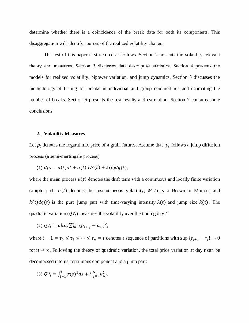
determine whether there is a coincidence of the break date for both its components. This

disaggregation will identify sources of the realized volatility change.

The rest of this paper is structured as follows. Section 2 presents the volatility relevant

theory and measures. Section 3 discusses data descriptive statistics. Section 4 presents the

models for realized volatility, bipower variation, and jump dynamics. Section 5 discusses the

methodology of testing for breaks in individual and group commodities and estimating the

number of breaks. Section 6 presents the test results and estimation. Section 7 contains some

conclusions.

2. Volatility Measures

Let denotes the logarithmic price of a grain futures. Assume that follows a jump diffusion

process (a semi-martingale process):

(1) ,

where the mean process denotes the drift term with a continuous and locally finite variation

sample path; denotes the instantaneous volatility; is a Brownian Motion; and

is the pure jump part with time-varying intensity and jump size . The

quadratic variation ( ) measures the volatility over the trading day :

(2)

,

where denotes a sequence of partitions with

for . Following the theory of quadratic variation, the total price variation at day can be

decomposed into its continuous component and a jump part:

(3)

,

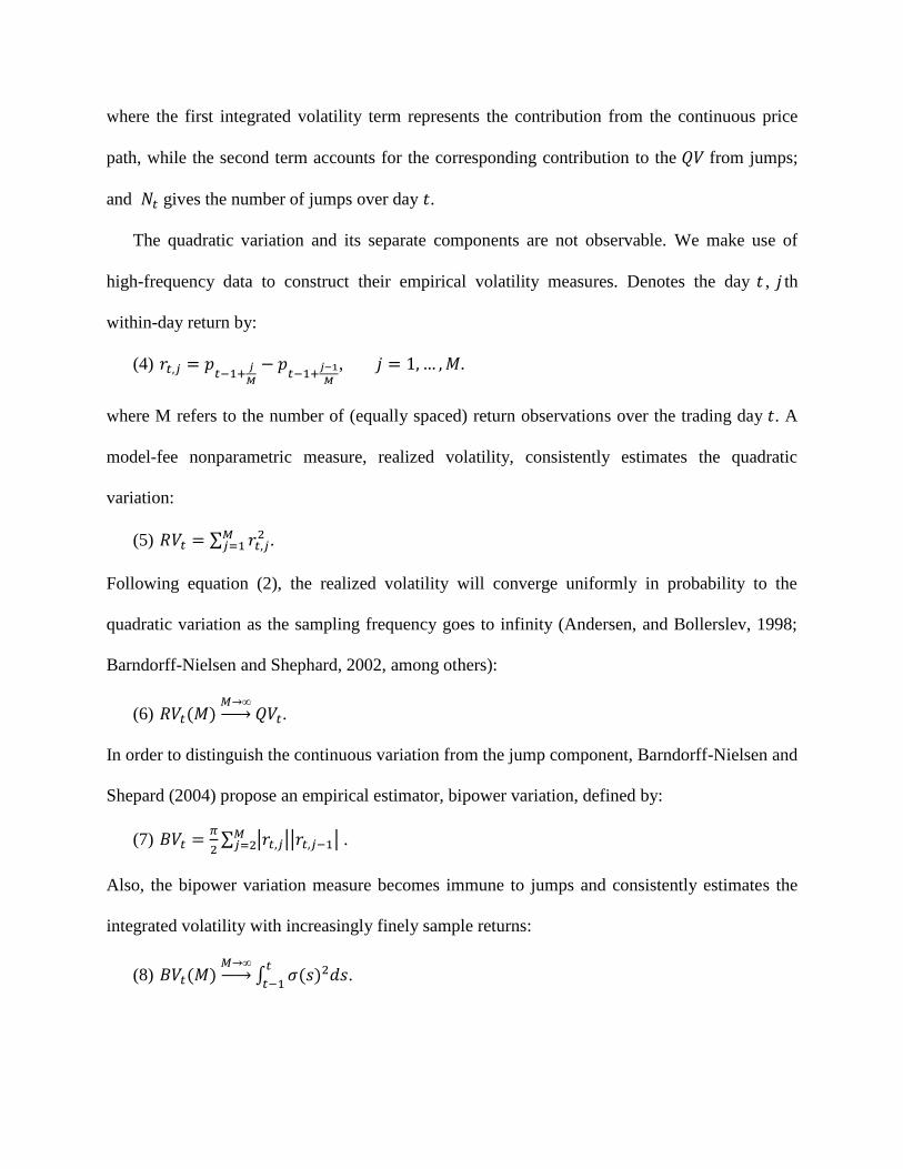
where the first integrated volatility term represents the contribution from the continuous price

path, while the second term accounts for the corresponding contribution to the from jumps;

and gives the number of jumps over day .

The quadratic variation and its separate components are not observable. We make use of

high-frequency data to construct their empirical volatility measures. Denotes the day , th

within-day return by:

(4)

,

where M refers to the number of (equally spaced) return observations over the trading day . A

model-fee nonparametric measure, realized volatility, consistently estimates the quadratic

variation:

(5)

.

Following equation (2), the realized volatility will converge uniformly in probability to the

quadratic variation as the sampling frequency goes to infinity (Andersen, and Bollerslev, 1998;

Barndorff-Nielsen and Shephard, 2002, among others):

(6) .

In order to distinguish the continuous variation from the jump component, Barndorff-Nielsen and

Shepard (2004) propose an empirical estimator, bipower variation, defined by:

(7)

.

Also, the bipower variation measure becomes immune to jumps and consistently estimates the

integrated volatility with increasingly finely sample returns:

(8)

.

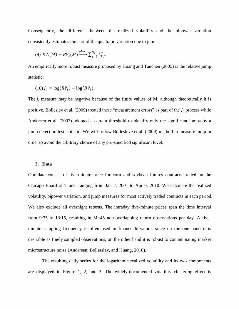
Consequently, the difference between the realized volatility and the bipower variation

consistently estimates the part of the quadratic variation due to jumps:

(9)

.

An empirically more robust measure proposed by Huang and Tauchen (2005) is the relative jump

statistic:

(10)

The measure may be negative because of the finite values of M, although theoretically it is

positive. Bolleslev et al. (2009) treated these ―measurement errors‖ as part of the process while

Andersen et al. (2007) adopted a certain threshold to identify only the significant jumps by a

jump detection test statistic. We will follow Bollesleve et al. (2009) method to measure jump in

order to avoid the arbitrary choice of any pre-specified significant level.

3. Data

Our data consist of five-minute price for corn and soybean futures contracts traded on the

Chicago Board of Trade, ranging from Jan 2, 2001 to Apr 6, 2010. We calculate the realized

volatility, bipower variation, and jump measures for most actively traded contracts in each period.

We also exclude all overnight returns. The intraday five-minute prices span the time interval

from 9:35 to 13:15, resulting in M=45 non-overlapping return observations per day. A five-

minute sampling frequency is often used in finance literature, since on the one hand it is

desirable as finely sampled observations, on the other hand it is robust to contaminating market

microstructure noise (Andersen, Bollerslev, and Huang, 2010).

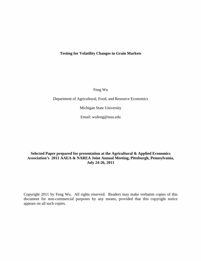
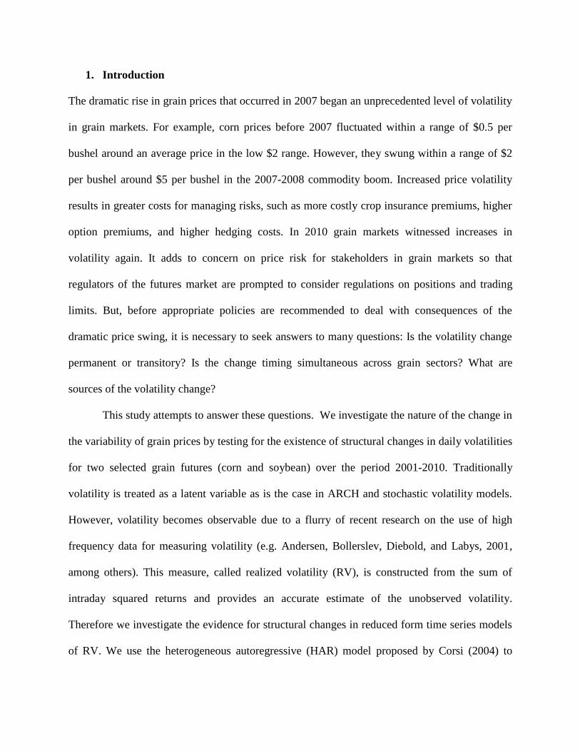
The resulting daily series for the logarithmic realized volatility and its two components

are displayed in Figure 1, 2, and 3. The widely-documented volatility clustering effect is

exhibited in each series. Also, the level of the logarithmic realized volatility exceeds that of the

logarithmic bipower variation series. In turn, the jump series depicted in the last panel exhibits

mostly positive values. It follows from Table 1 that the unconditional distributions of both the

logarithmic continuous volatility measures are approximately normal. However, the descriptive

statistics for the relative jump measure clearly indicate a positively skewed and leptokurtic

distribution. Turning to the lower panel in the table, all of the volatility measures exhibit highly

significant own serial dependencies, as evidenced by the Ljung-box test statistics for up to 20th

order autocorrelation. It is consistent with the widely-documented long memory feature in the

literature. Meanwhile, the relative jump measure also exhibits similar long-memory

characteristics. In contrast, much less autocorrelation exists in S&P500 index time series.

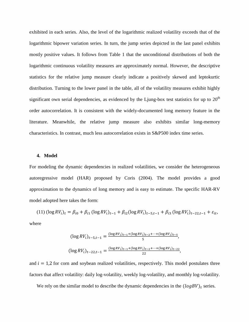
4. Model

For modeling the dynamic dependencies in realized volatilities, we consider the heterogeneous

autoregressive model (HAR) proposed by Coris (2004). The model provides a good

approximation to the dynamics of long memory and is easy to estimate. The specific HAR-RV

model adopted here takes the form:

(11) ,

where

,

,

and for corn and soybean realized volatilities, respectively. This model postulates three

factors that affect volatility: daily log-volatility, weekly log-volatility, and monthly log-volatility.

We rely on the similar model to describe the dynamic dependencies in the series.

(12) .

The descriptive statistics point toward fairly strong own serial autocorrelations in the relative

jump series. To best accommodate the feature in the model, we specify a HAR-J model:

(13) ,

where

,

.

In the jump dynamics, the lagged jumps are generally insignificant. Other regressors, such as

weekly and monthly log(BV), are also taken into account but omitted from the model due to the

insignificance. Finally, the Ljung-box Q-statistics for all absolute residuals reveal no significant

auto-correlations. 2

5. Estimation and Test

We follow a setup in the Bai and Perron methodology to test for existence, number, and timing

of the breaks in individual commodity realized volatility time series. The procedure is as follows.

We estimate the linear equations for different sets of intercepts and slopes corresponding to

different combinations of break points. The break date is pin down by obtaining global

minimizers of the sum of squared residuals. An F-test is constructed to examine if there is a

statistically significant break. If the null hypothesis of no break is rejected, we continue to

determine the exact number and their location by the so-called sequential method. The method

2 But the Ljung-Box Q-statistics for the squared realized volatility and bipower variation residuals reveal clear

evidence for significant conditional heteroskedasticity. We didn’t augment the basic model with a GARCH error

structure for the time-varying volatility of volatility, since on the one hand coefficient estimates are only limitedly

improved, on the other hand in the break test, whether Bai and Perron test or Qu and Perron test, are robust to

heteroskedasticity.

adds one break each time the F-test is significant. The detailed theory on estimating and testing a

single equation with multiple structural changes can be found in Bai and Perron (1998). Bai and

Perron (2003) demonstrated the empirical application of the procedures. More statement will be

placed on the Qu and Perron method, which proposed a general framework to test structural

changes in multivariate regressions. Furthermore, it has not yet been applied too much. In fact,

our study is one of the empirical applications of it.3

To test the common break in grouped realized volatilities, we cast the model (11) into an

alternative form proposed by Qu and Perron (2007):

(14) ,

where , is the set that includes the regressors from two

equations. A subscript j indexes a regime (j=1,2,…,m+1) when the total number of common

structural breaks in the system is m. We denote the break dates by the m vector

and set that and . The matrix S is a selection matrix having dimension 14

that involves elements with 0 or 1to specify which regressors appear in each equation. has

mean 0 and covariance matrix for We define the

matrix by so that (14) becomes

(15)

Qu and Perron (2007) applied a quasi-maximum likelihood method based on normal errors to

estimate multiple structural changes that occur at unknown dates in a system of equations. This is

a fairly general method with the following flexibilities: a) allowing changes in the coefficients of

the conditional mean; b) allowing changes in the coefficients of the covariance matrix of the

residuals; and c) allowing arbitrary restrictions on these parameters so that we can analyze not

3 We are also gateful to Jushan Bai, Pierre Perron, and Zhongjun Qu for making their GAUSS programs available.

only common breaks that occur in all equations, but also breaks that occur in a subset of

equations. Given the partition of the sample , the system’s quasi-likelihood

function is

(16)

,

where is a multivariate normal distribution. Thus the quasi-likelihood ratio is

(17)

,

where a 0 subscript denotes the true value of the parameters. Then the parameter estimates are to

maximize a log-likelihood ratio with parameter restrictions:

(18) ,

where is a restriction on parameters.

Qu and Perron (2007) have corroborated that the log-likelihood ratio optimization

problem can be split into two asymptotically independent components so that the estimates of the

break dates and the coefficients ( are unaffected each other. Furthermore, the restrictions

on parameters do not also affect the distribution of the break dates. Under the theorem, the

limiting distribution of the estimates of the break dates are easily derived (See theorem 2 and 3 in

Qu and Perron (2007)).

To construct the QMLE, a general algorithm to the optimization problem (18) is a grid

search, but it is no longer feasible in the computation of maximum likelihood estimate of order

Qu and Perron (2006) used a dynamic programming algorithm identical to Bai and

Perron (2003). The main idea is to first calculate the overall value of the log-likelihood function

for all possible segments, and then use this algorithm to assess which particular combination of

m+1 segments leads to the highest likelihood value.

After estimating the break dates by QMLE, a likelihood ratio statistic is constructed o test

the null hypothesis with no change in any of the coefficients versus an alternative hypothesis

with a pre-specified number of changes. The test statistic is

(19) ,

where

,

and

.

A tilde subscript denotes the parameter estimates under the null hypothesis (no change in

structure), while a delta subscript denotes the parameter estimates under the alternative

hypothesis (m structural changes in the system). If no change occurs, the QMLE is equivalent to

the generalized least squares estimate, and thus other coefficients can be estimated as

,

.

The estimates can be obtained by beginning with the OLS of estimates of coefficients in the

mean equation and iterate until convergence. Under the alternative hypothesis, the QMLE jointly

solve the equations

,

.

The estimates allow the structure change occurring in the conditional mean and the covariance

matrix of the errors. The limiting distribution of the test statistic is derived by Qu and Perron

(2007) and depends on the number of regressors whose coefficients are allowed to change, the

number of coefficients of the covariance matrix allowed to change, and the distribution the errors.

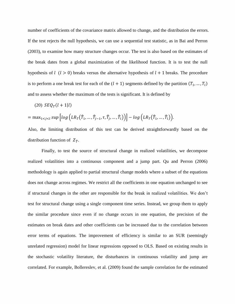
If the test rejects the null hypothesis, we can use a sequential test statistic, as in Bai and Perron

(2003), to examine how many structure changes occur. The test is also based on the estimates of

the break dates from a global maximization of the likelihood function. It is to test the null

hypothesis of breaks versus the alternative hypothesis of breaks. The procedure

is to perform a one break test for each of the ( segments defined by the partition

and to assess whether the maximum of the tests is significant. It is defined by

(20)

.

Also, the limiting distribution of this test can be derived straightforwardly based on the

distribution function of .

Finally, to test the source of structural change in realized volatilities, we decompose

realized volatilities into a continuous component and a jump part. Qu and Perron (2006)

methodology is again applied to partial structural change models where a subset of the equations

does not change across regimes. We restrict all the coefficients in one equation unchanged to see

if structural changes in the other are responsible for the break in realized volatilities. We don’t

test for structural change using a single component time series. Instead, we group them to apply

the similar procedure since even if no change occurs in one equation, the precision of the

estimates on break dates and other coefficients can be increased due to the correlation between

error terms of equations. The improvement of efficiency is similar to an SUR (seemingly

unrelated regression) model for linear regressions opposed to OLS. Based on existing results in

the stochastic volatility literature, the disturbances in continuous volatility and jump are

correlated. For example, Bollereslev, et al. (2009) found the sample correlation for the estimated

residuals from the Bipower variation and jump equations are -0.1847. Additionally, they also

find there might exist nonlinear dependencies—a smirk-like relation between the innovations to

the continuous volatility and jump components. Testing for a structural change in a system of

equations because of interdependencies between disturbances would obviously improve

estimation efficiency.

6. Results

First, we use the Bai and Perron (1998, 2003) method to estimate multiple breaks in individual

grain commodity time series. At each step, according to the recommendation of Bai and Perron

(2006), we test the null hypothesis of no breaks against an unknown number of breaks. If the null

of no breaks is rejected, we use the sequential test to determine the number of and locations of

breaks. Table 2 reports the test statistics and the 90% confidence interval for the break date

estimates. Two interesting results are revealed from Table 2. Firstly, the tests suggest that

there is evidence of structural changes in the coefficients that govern the dynamics of realized

volatilities for corn and soybean. We reject the null of no break in favor of the alternative of

breaks. Secondly, the sequential tests suggest that only one structural change occurs in the

soybean and corn volatilities. The break date for corn is estimated at Nov 18, 2006, while the

date for soybean is estimated at one year later. Table 3 and 4 give other coefficient estimates for

corn and soybean HAR models. The coefficient estimates show predictive ability of regressors

has similar change for corn and soybean: in the second regime, weekly log-realized volatilities

reduce its weight on the prediction while monthly log-realized volatilities increase its effect. This

means in recent years long memory feature of these two commodities has become more

prominent.

Next, we test whether there is a common structural break between the corn and soybean

realized volatilities using the Qu and Perron test in a system of two equations. That is, we see

whether the difference of break dates for corn and soybean is negligible in statistics. This

approach restricts the breaks to occurring at the same time in both equations and therefore can

detect breaks in the ratio when they occur in the component series simultaneously but with

different magnitudes. Our test results indicate that there is little evidence of a common structural

change in the corn and soybean realized volatilities. The test for 0 versus 1.000 break is

18.486, while the 10% and 5% significance levels are 20.78 and 23.21. In short, there are no

common structural changes between corn and soybean realized volatilities.

To further investigate the source of realized volatilities in each commodity, we turn to the

system of equations composed by the bipower variation and jump. We apply the same empirical

methods as the case in the system of realized volatilities. Table 5 describes the test results. First

we allow breaks in all the regression coefficients. The SupF test for the structural changes

suggests one common structural change in corn bipower and jump time series. But the break date

is prior to the date found in the single realized volatility series. The break date estimate is Feb 8,

2006, and the 90 percent confidence interval is Dec 7, 2005 to April 10, 2006. There is no

evidence of a second structural break in the system. As for soybean, there is evidence of

structural change. Furthermore, the break date estimate is almost exactly same as the case in the

soybean realized volatilities. In order to check the timing of the structural break simultaneous

across components, we restrict coefficients in one subset of equation unchanged. When

coefficients in jump series is unchanged in the two regimes, we found the SupF test can not

reject the null hypothesis, that is, there is no evidence of structural change in the bipower

variation series regardless of corn or soybean. But if we keep coefficients in bipower variation

series unchanged, the test rejects the null hypothesis and there is a remarkable coincidence of the

break date for the system of jump and bipower variation as a whole with and without restrictions.

The statistical significance is very strong for soybean, say, 1% level, while it is about relatively

weak for corn, say, 10% level. Apparently, the structural change in the realized volatilities for

corn and soybean is due to roughly simultaneous breaks in the jump series.

7. Conclusion

We use newly nonparametric volatility measures and break techniques to estimate common

breaks across grain futures over the recent ten years. Our results show one structural change in

realized volatilities occurred in 2006 for corn and in 2007 for soybean. But the date difference

between them cannot be negligible. We disaggregate the realized volatilities into a continuous

component and a jump part and found the source of structural beak in realized volatilities is from

jumps.

Reference:

Andersen, T.G., Bollerslev, T. 1998. ―Answering the skeptics: yes, standard volatility models do

provide accurate forecasts.‖ International Economic Review 39, 885-905.

Andersen, T.G., Bollerslev, T., Diebold, F.X., Labys, P. 2001. ―The distribution of exchange rate

volatility.‖ Journal of the American Statistical Association 96, 42-55.

Andersen, T.G., Bollerslev, T., Diebold, F.X. 2007. ―Roughing it up: Including jump

components in the measurement, modeling and forecasting of return volatility.‖ Review of

Economics and Statistics 89 (4), 701-720

Andersen, T.G., et al. 2010. ―A reduced form framework for modeling volatility of speculative

prices based on realized variation measures.‖ Journal of Econometrics,

doi:10.1016/j.jeconom.2010.03.029.

Bai, Jushan, and Pierre Perron, 1998. ―Estimating and Testing Linear Models with Multiple

Structural Changes.‖ Econometrica 66, 47– 78.

——— 2003. ―Computation and Analysis of Multiple Structural Change Models.‖ Journal of

Applied Econometrics 18, 1–22.

Barndorff-Nielsen, Ole E., Shephard, Neil. 2006. ―Econometrics of testing for jumps in financial

economics using bipower variation.‖ Journal of Financial Econometrics 4, 1-30.

Bollerslev, Tim, Kretschmer, Uta, Pigorsch, Christian, Tauchen, George. 2009. ―A discrete-time

model for daily S&P 500 returns and realized variations: jumps and leverage effects.‖

Journal of Econometrics 150,151-166.

Corsi, Fulvio, 2004. ―A simple long memory model of realized volatility.‖ Working Paper.

University of Lugano.

Liu Chun and John M. Maheu. 2008. ―Are there Structural Breaks in Realized Volatility?‖

Journal of Financial Econometrics 6 (3), 326-360.

Qu, Zhongjun, and Pierre Perron. 2007. ―Estimating and Testing Multiple Structural Changes in

Multivariate Regressions.‖ Econometrica 75, 459–502.

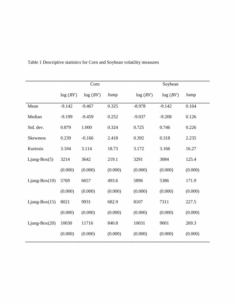
Table 1 Descriptive statistics for Corn and Soybean volatility measures

Corn Soybean

Jump Jump

Mean -9.142 -9.467 0.325 -8.978 -9.142 0.164

Median -9.199 -9.459 0.252 -9.037 -9.208 0.126

Std. dev. 0.879 1.000 0.324 0.725 0.746 0.226

Skewness 0.239 -0.166 2.418 0.392 0.318 2.235

Kurtosis 3.104 3.114 18.73 3.172 3.166 16.27

Ljung-Box(5) 3214

(0.000)

3642

(0.000)

219.1

(0.000)

3291

(0.000)

3084

(0.000)

125.4

(0.000)

Ljung-Box(10) 5769

(0.000)

6657

(0.000)

493.6

(0.000)

5896

(0.000)

5386

(0.000)

171.9

(0.000)

Ljung-Box(15) 8021

(0.000)

9931

(0.000)

682.9

(0.000)

8107

(0.000)

7311

(0.000)

227.5

(0.000)

Ljung-Box(20) 10030

(0.000)

11716

(0.000)

840.8

(0.000)

10031

(0.000)

9001

(0.000)

269.3

(0.000)

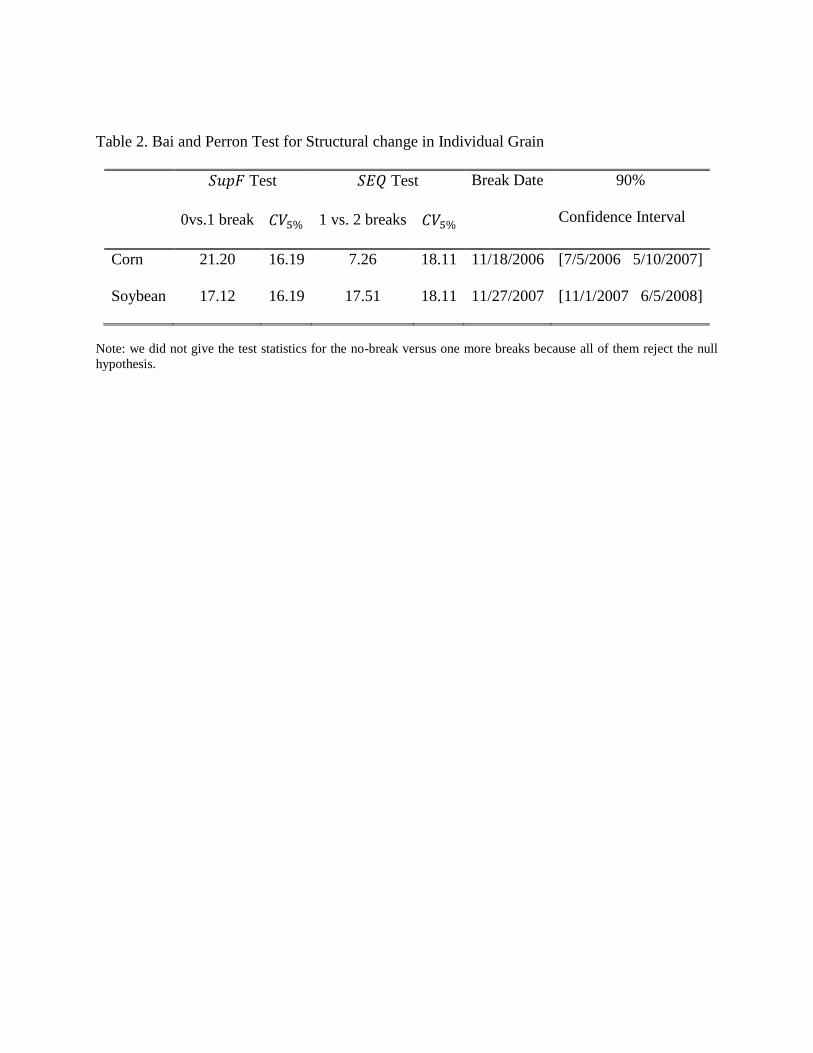
Table 2. Bai and Perron Test for Structural change in Individual Grain

Test Test Break Date 90%

Confidence Interval 0vs.1 break 1 vs. 2 breaks

Corn 21.20 16.19 7.26 18.11 11/18/2006 [7/5/2006 5/10/2007]

Soybean 17.12 16.19 17.51 18.11 11/27/2007 [11/1/2007 6/5/2008]

Note: we did not give the test statistics for the no-break versus one more breaks because all of them reject the null

hypothesis.

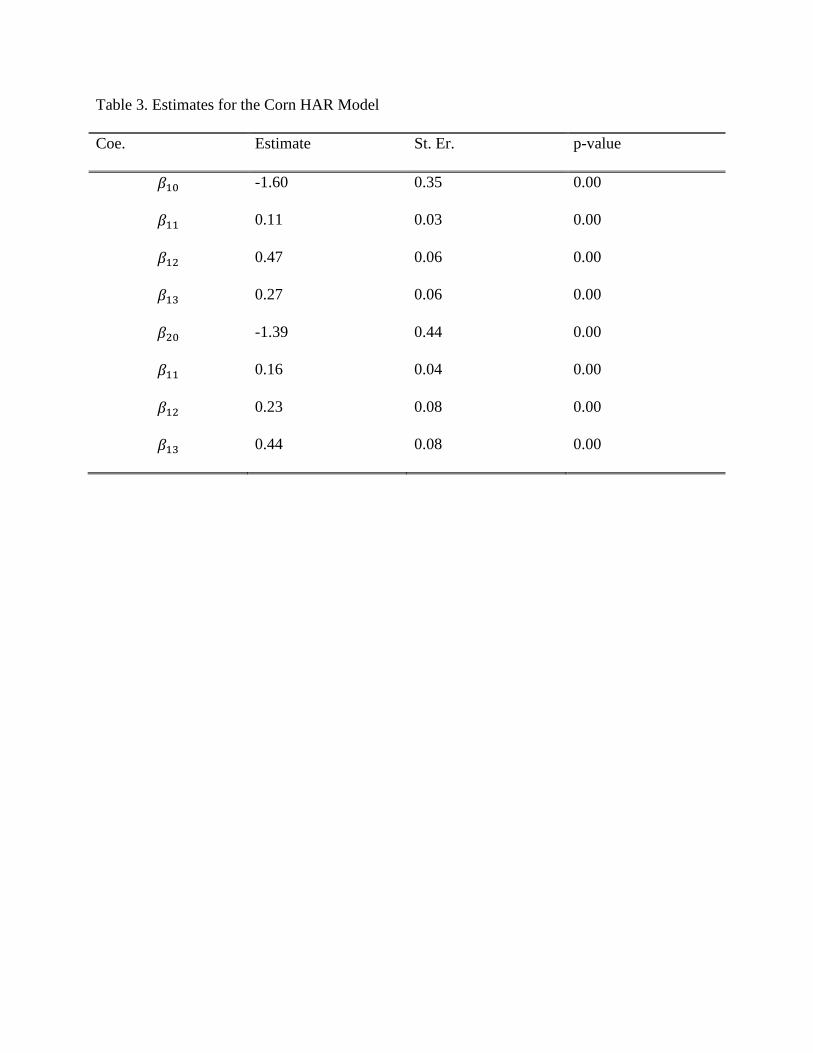
Table 3. Estimates for the Corn HAR Model

Coe. Estimate St. Er. p-value

-1.60 0.35 0.00

0.11 0.03 0.00

0.47 0.06 0.00

0.27 0.06 0.00

-1.39 0.44 0.00

0.16 0.04 0.00

0.23 0.08 0.00

0.44 0.08 0.00

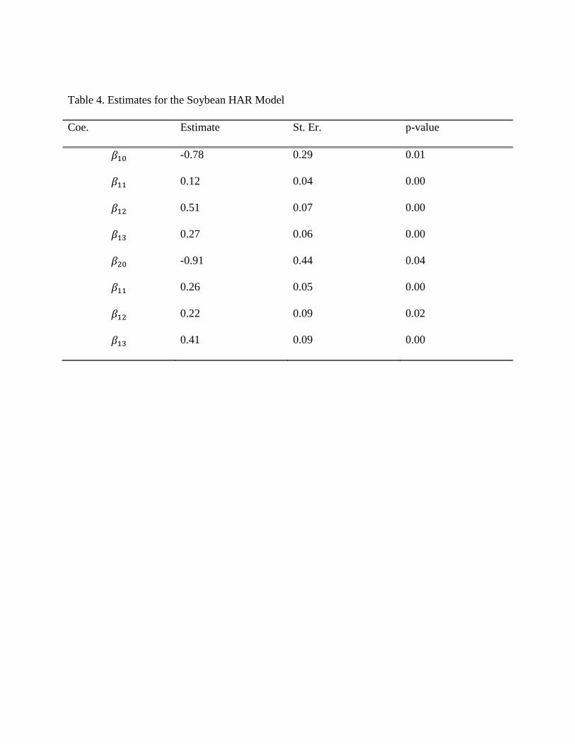
Table 4. Estimates for the Soybean HAR Model

Coe. Estimate St. Er. p-value

-0.78 0.29 0.01

0.12 0.04 0.00

0.51 0.07 0.00

0.27 0.06 0.00

-0.91 0.44 0.04

0.26 0.05 0.00

0.22 0.09 0.02

0.41 0.09 0.00

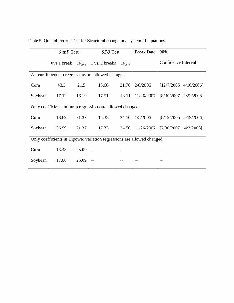
Table 5. Qu and Perron Test for Structural change in a system of equations

Test Test Break Date 90%

Confidence Interval 0vs.1 break 1 vs. 2 breaks

All coefficients in regressions are allowed changed

Corn 48.3 21.5 15.68 21.70 2/8/2006 [12/7/2005 4/10/2006]

Soybean 17.12 16.19 17.51 18.11 11/26/2007 [8/30/2007 2/22/2008]

Only coefficients in jump regressions are allowed changed

Corn 18.89 21.37 15.33 24.50 1/5/2006 [8/19/2005 5/19/2006]

Soybean 36.99 21.37 17.33 24.50 11/26/2007 [7/30/2007 4/3/2008]

Only coefficients in Bipower variation regressions are allowed changed

Corn 13.48 25.09 -- -- -- --

Soybean 17.06 25.09 -- -- -- --

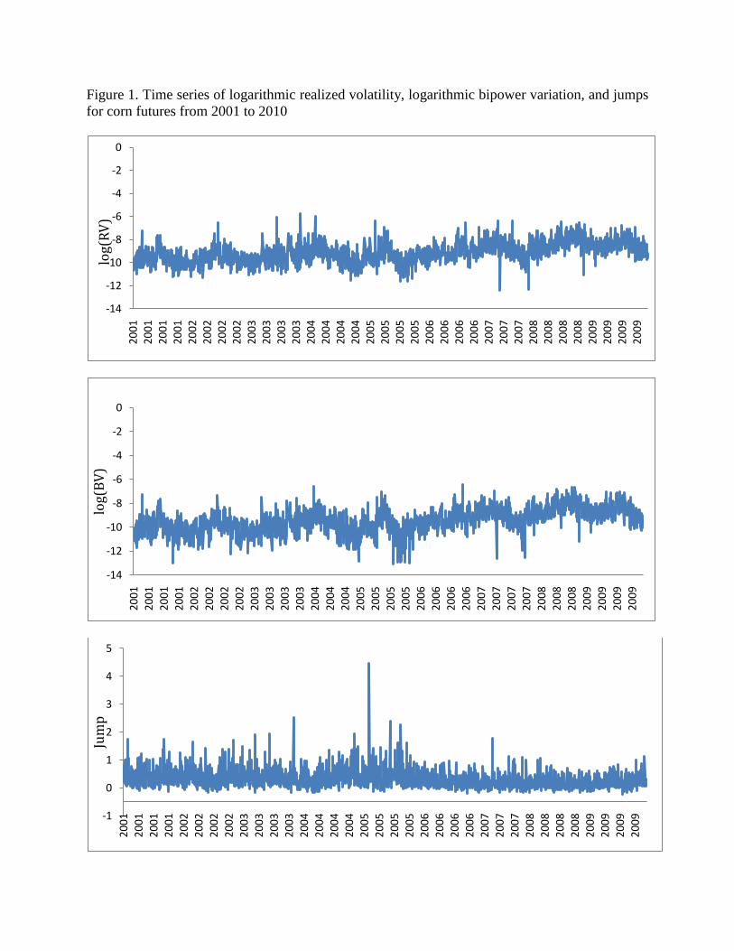
Figure 1. Time series of logarithmic realized volatility, logarithmic bipower variation, and jumps

for corn futures from 2001 to 2010

-14

-12

-10

-8

-6

-4

-2

02

00

12

00

12

00

12

00

12

00

22

00

22

00

22

00

22

00

32

00

32

00

32

00

32

00

42

00

42

00

42

00

42

00

52

00

52

00

52

00

52

00

62

00

62

00

62

00

62

00

72

00

72

00

72

00

82

00

82

00

82

00

82

00

92

00

92

00

92

00

9

log(RV)

-14

-12

-10

-8

-6

-4

-2

0

20

01

20

01

20

01

20

01

20

02

20

02

20

02

20

02

20

03

20

03

20

03

20

03

20

04

20

04

20

04

20

05

20

05

20

05

20

05

20

06

20

06

20

06

20

06

20

07

20

07

20

07

20

07

20

08

20

08

20

08

20

09

20

09

20

09

20

09

log(BV)

-1

0

1

2

3

4

5

20

01

20

01

20

01

20

01

20

02

20

02

20

02

20

02

20

03

20

03

20

03

20

03

20

04

20

04

20

04

20

04

20

05

20

05

20

05

20

05

20

06

20

06

20

06

20

06

20

07

20

07

20

07

20

08

20

08

20

08

20

08

20

09

20

09

20

09

20

09

Jump

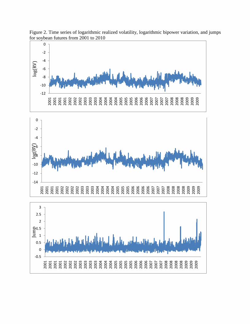
Figure 2. Time series of logarithmic realized volatility, logarithmic bipower variation, and jumps

for soybean futures from 2001 to 2010

-12

-10

-8

-6

-4

-2

0

20

01

20

01

20

01

20

01

20

02

20

02

20

02

20

03

20

03

20

03

20

04

20

04

20

04

20

04

20

05

20

05

20

05

20

06

20

06

20

06

20

07

20

07

20

07

20

07

20

08

20

08

20

08

20

09

20

09

20

09

log(RV)

-14

-12

-10

-8

-6

-4

-2

0

20

01

20

01

20

01

20

01

20

02

20

02

20

02

20

02

20

03

20

03

20

03

20

04

20

04

20

04

20

04

20

05

20

05

20

05

20

06

20

06

20

06

20

06

20

07

20

07

20

07

20

08

20

08

20

08

20

08

20

09

20

09

20

09

log(BV)

-0.5

0

0.5

1

1.5

2

2.5

3

20

01

20

01

20

01

20

01

20

02

20

02

20

02

20

03

20

03

20

03

20

03

20

04

20

04

20

04

20

05

20

05

20

05

20

05

20

06

20

06

20

06

20

07

20

07

20

07

20

08

20

08

20

08

20

08

20

09

20

09

20

09

Jump