0

TESTING FOR SERIAL CORRELATION: GENERALIZED ANDREWS-PLOBERGER TESTS

John C. Nankervis

Essex Finance Centre, Essex Business School

University of Essex, Colchester, CO4 3SQ U.K.

N. E. Savin

Department of Economics, University of Iowa, Iowa City, IA 52242.

August 16, 2008

ABSTRACT

This paper considers testing the null hypothesis that a times series is uncorrelated

when the time series is uncorrelated but statistically dependent. This case is of interest in

economic and finance applications. The GARCH (1, 1) model is a leading example of a

model that generates serially uncorrelated but statistically dependent data. The tests of

serial correlation introduced by Andrews and Ploberger (1996, hereafter AP) are

generalized for the purpose of testing the null. The rationale for generalizing the AP tests

is that they have attractive properties for case for which they were originally designed:

They are consistent against all non-white noise alternatives and have good all-round

power against nonseasonal alternatives compared to several widely used tests in the

literature. These properties are inherited by the generalized AP tests.

JEL classification: C12; C22

Keywords: Autoregressive moving average model; Lagrange multiplier test; Nonstandard testing; Statistically dependent time series; Uncorrelatedness. Corresponding author: N. E. Savin, Department of Economics, 108 Pappajohn Business Building, Iowa City, IA 52242-1994. Tel.: (319) 335-0855; fax: (319) 335-1956. Email address: gene-savin@uiowa.edu.

1

1. INTRODUCTION

As noted by Hong and Lee (2003), there has been growing interest in developing

consistent tests for serial correlation of unknown form; examples include AP, Hong

(1996), Chen and Deo (2004) in estimated regression residuals and Durlauf (1991) and

Deo (2000) in the observed raw data. The tests assume independently and identically

distributed regression errors under the null except for Deo (2000), which generalizes

Durlauf (1991) to allow for a restrictive form of conditional heteroskedasticity. This

paper considers testing the null that a times series is uncorrelated when the time series is

uncorrelated but statistically dependent. For a more extensive literature review, see

Francq, Roy and Zakoian (2005).

The case of uncorrelated dependent time series is of interest in economic and

financial applications because many problems such as financial (non-) predictability are

related to a martingale difference sequence (MDS) hypothesis after demeaning, which

implies serial uncorrelatedness but not serial independence. The GARCH (1, 1) model is

a leading example of a model that generates serially uncorrelated but statistically

dependent data. The rationale for generalizing the AP tests is that they are consistent

against all non-white noise alternatives and have good all-round power against

nonseasonal alternatives when compared to several tests in the literature, including the

Box-Pierce (1970, hereafter BP) tests. The generalized AP tests inherit the properties of

the AP tests in power comparisons. In our simulation experiments, the generalized AP

tests typically have substantially better power than the generalized BP (Lobato,

Nankervis and Savin (2002)) tests against non-seasonal alternatives and power equal to or

better than the Deo (2000) test.

2

AP introduced tests of serial correlation designed for the case where the time

series is generated by ARMA (1, 1) models under the alternative. As they noted, it is

natural to consider tests of this sort because ARMA (1, 1) models provide parsimonious

representations of a broad class of stationary time series. ARMA(1, 1) models for

financial returns series follow from the mean-reversion models of Poterba and Summers

(1988) and the price-trend models of Taylor (2005). However, testing for serial

correlation generated by an ARMA (1, 1) model is a nonstandard testing problem because

the ARMA (1, 1) model reduces to a white noise model whenever the AR and MA

coefficients are equal. The testing problem is one in which a nuisance parameter is

present only under the alternative hypothesis. For the problem addressed by AP, the

standard likelihood ratio (LR) statistic does not possess its usual asymptotic chi-squared

distribution or its usual asymptotic optimality properties. It is also possible that an

ARMA(1,1) generates white noise when the AR and MA coefficients are not equal, as is

the case for the all-pass filter model; see Andrews, Davis and Breidt (2006).

The LR test has the attractive feature of being consistent against all forms of serial

correlation (Potscher (1990)). AP show that this feature also holds for tests introduced

into the literature by Andrews and Ploberger (1994, 1995), namely, the sup Lagrange

Multiplier (LM) and average exponential LM and LR tests. AP establish the asymptotic

null distribution for the LR, sup LM and average exponential test statistics under the

assumption that the generating process is a conditionally homoskedastic martingale

difference sequence (MDS). The asymptotic critical values for these tests were

calculated by simulation. In Monte Carlo power experiments, AP compared the finite-

sample powers of the LR, sup LM, average exponential, BP, and other tests. The

3

alternatives include Gaussian ARMA (1, 1) models. Against this class of alternatives, the

LR test was found to have very good all-around power properties for non-seasonal

alternative models, especially compared to BP tests.

For serially uncorrelated but statistically dependent time series, the true levels of

the LR, sup LM and average exponential tests can differ substantially from the nominal

levels when the tests use the asymptotic critical values calculated by AP. This paper

generalizes a subset of the tests considered by AP so that they have the correct level

asymptotically when the time series is serially uncorrelated but statistically dependent.

The subset consists of LM-based tests, namely the sup LM test and the average

exponential LM tests. The generalization is obtained by using the true asymptotic

covariance matrix of the sample autocorrelations, or a consistent estimator. The same

approach has been used by Lobato, Nankervis and Savin (2002) to generalize the BP tests

to settings where the time series is serially uncorrelated but statistically dependent. The

asymptotic critical values reported by AP remain valid for the generalized LM-based

tests.

The finite-sample levels of the generalized LM-based tests with asymptotic

critical values are assessed by simulation. In Monte Carlo power experiments, these tests

are compared to generalized BP tests and the Deo (2000) test. The generalized AP tests

typically have better level-corrected power against non-seasonal alternatives. Hence,

generalized AP tests can be recommended for use in economic and finance applications.

The paper reports the results of an empirical application to stock return indexes.

2. ARMA (1, 1) MODEL AND TEST STATISTICS This section reviews the model, hypothesis and test statistics considered by AP.

4

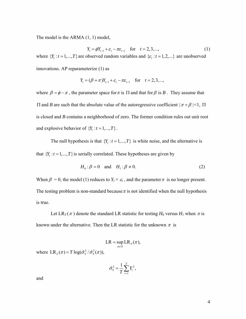
The model is the ARMA (1, 1) model, 1 1 for 2,3,...,t t t tY Y tφ ε πε− −= + − = (1) where { : 1,..., }tY t T= are observed random variables and { : 1,2,...}t tε = are unobserved

innovations. AP reparameterize (1) as

1 1( ) for 2,3,...,t t t tY Y tβ π ε πε− −= + + − = where β φ π= − , the parameter space forπ is Π and that for β is B . They assume that

Π and B are such that the absolute value of the autoregressive coefficient | |π β+ <1, Π

is closed and B contains a neighborhood of zero. The former condition rules out unit root

and explosive behavior of { : 1,..., }tY t T= .

The null hypothesis is that { : 1,..., }tY t T= is white noise, and the alternative is

that { : 1,..., }tY t T= is serially correlated. These hypotheses are given by

0 1: 0 and : 0.H Hβ β= ≠ (2) When β = 0, the model (1) reduces to Yt = εt , and the parameterπ is no longer present.

The testing problem is non-standard becauseπ is not identified when the null hypothesis

is true.

Let LRT (π ) denote the standard LR statistic for testing H0 versus H1 when π is

known under the alternative. Then the LR statistic for the unknown π is

LR sup LR ( ),T

ππ

∈Π=

where 2 2ˆLR ( ) log( / ( )),T Y YTπ σ σ π=

2 2

1

1 ,T

Y tt

YT

σ=

= ∑

and

5

2 22 2

2 21 1

2 0 2 0

1ˆ ( ) .T t T t

i iY Y t t i t i

t i t i

Y Y YT

σ π σ π π− −

− − − −= = = =

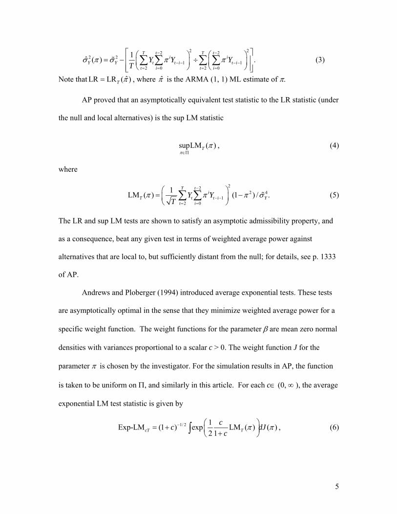
⎡ ⎤⎛ ⎞ ⎛ ⎞= − ÷⎢ ⎥⎜ ⎟ ⎜ ⎟⎝ ⎠ ⎝ ⎠⎢ ⎥⎣ ⎦∑ ∑ ∑ ∑ (3)

Note that ˆLR LR ( )T π= , where π̂ is the ARMA (1, 1) ML estimate of π.

AP proved that an asymptotically equivalent test statistic to the LR statistic (under

the null and local alternatives) is the sup LM statistic

supLM ( )T

ππ

∈Π, (4)

where

22

2 41

2 0

1LM ( ) (1 ) / .T t

iT t t i Y

t iY Y

Tπ π π σ

−

− −= =

⎛ ⎞= −⎜ ⎟

⎝ ⎠∑ ∑ (5)

The LR and sup LM tests are shown to satisfy an asymptotic admissibility property, and

as a consequence, beat any given test in terms of weighted average power against

alternatives that are local to, but sufficiently distant from the null; for details, see p. 1333

of AP.

Andrews and Ploberger (1994) introduced average exponential tests. These tests

are asymptotically optimal in the sense that they minimize weighted average power for a

specific weight function. The weight functions for the parameter β are mean zero normal

densities with variances proportional to a scalar c > 0. The weight function J for the

parameter π is chosen by the investigator. For the simulation results in AP, the function

is taken to be uniform on Π, and similarly in this article. For each c∈ (0, ∞ ), the average

exponential LM test statistic is given by

1/ 2 1Exp-LM (1 ) exp LM ( ) ( )2 1cT T

cc dJc

π π− ⎛ ⎞= + ⎜ ⎟+⎝ ⎠∫ , (6)

6

where LMT (π) is as defined in (5), and J(⋅) is probability measure on Π. The average

exponential LR test statistic, Exp-LRcT, is defined analogously with LMT (π) being

replaced by LRT (π). The limiting average exponential LM test statistics as 0c → and

c → ∞ are given by

0Exp-LM = LM ( ) ( )T T dJπ π∫ and

1Exp-LM ln exp LM ( ) ( )2T T dJπ π∞

⎛ ⎞= ⎜ ⎟⎝ ⎠∫ . (7)

Andrews and Ploberger (1994) show that the average exponential tests have asymptotic

local power optimality properties.

3. ASYMPTOTIC AND FINITE-SAMPLE NULL DISTRIBUTIONS OF AP TEST STATISTICS AP established the asymptotic null distribution of the test statistics previously

introduced. This section reviews the asymptotic theory.

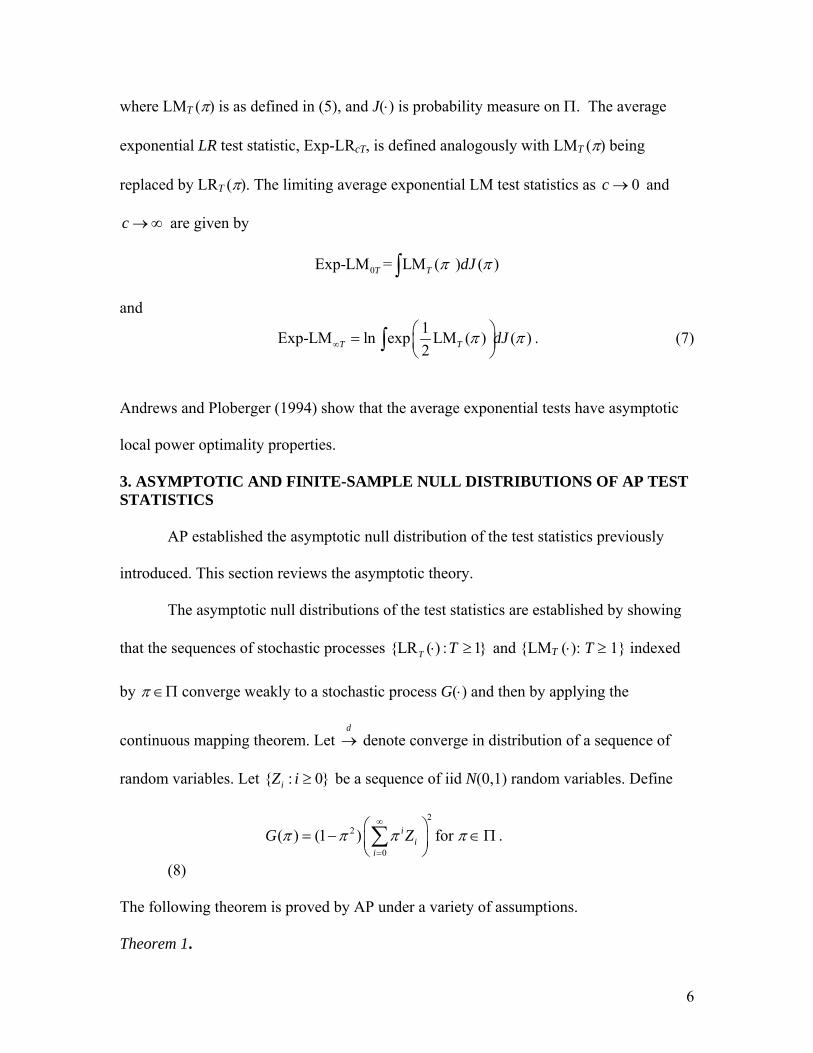
The asymptotic null distributions of the test statistics are established by showing

that the sequences of stochastic processes {LR ( ) : 1}T T⋅ ≥ and {LMT (⋅): T ≥ 1} indexed

by π ∈Π converge weakly to a stochastic process G(⋅) and then by applying the

continuous mapping theorem. Let d

→ denote converge in distribution of a sequence of

random variables. Let { : 0}iZ i ≥ be a sequence of iid N(0,1) random variables. Define

2

2

0

( ) (1 ) forii

i

G Zπ π π π∞

=

⎛ ⎞= − ∈Π⎜ ⎟⎝ ⎠∑ .

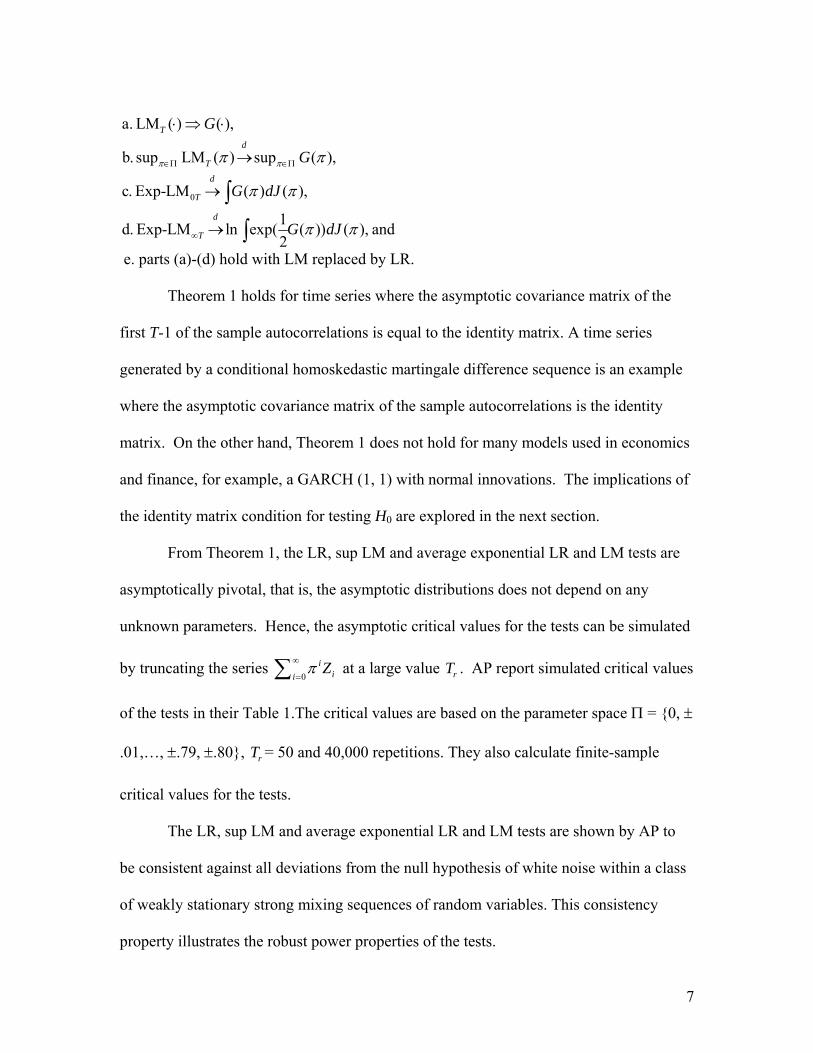
(8) The following theorem is proved by AP under a variety of assumptions. Theorem 1.

7

0

a. LM ( ) ( ),

b. sup LM ( ) sup ( ),

c. Exp-LM ( ) ( ),

1d. Exp-LM ln exp( ( )) ( ), and2

Td

T

d

T

d

T

G

G

G dJ

G dJ

π ππ π

π π

π π

∈Π ∈Π

∞

⋅ ⇒ ⋅

→

→

→

∫

∫

e. parts (a)-(d) hold with LM replaced by LR.

Theorem 1 holds for time series where the asymptotic covariance matrix of the

first T-1 of the sample autocorrelations is equal to the identity matrix. A time series

generated by a conditional homoskedastic martingale difference sequence is an example

where the asymptotic covariance matrix of the sample autocorrelations is the identity

matrix. On the other hand, Theorem 1 does not hold for many models used in economics

and finance, for example, a GARCH (1, 1) with normal innovations. The implications of

the identity matrix condition for testing H0 are explored in the next section.

From Theorem 1, the LR, sup LM and average exponential LR and LM tests are

asymptotically pivotal, that is, the asymptotic distributions does not depend on any

unknown parameters. Hence, the asymptotic critical values for the tests can be simulated

by truncating the series 0

iii

Zπ∞

=∑ at a large value rT . AP report simulated critical values

of the tests in their Table 1.The critical values are based on the parameter space Π = {0, ±

.01,…, ±.79, ±.80}, rT = 50 and 40,000 repetitions. They also calculate finite-sample

critical values for the tests.

The LR, sup LM and average exponential LR and LM tests are shown by AP to

be consistent against all deviations from the null hypothesis of white noise within a class

of weakly stationary strong mixing sequences of random variables. This consistency

property illustrates the robust power properties of the tests.

8

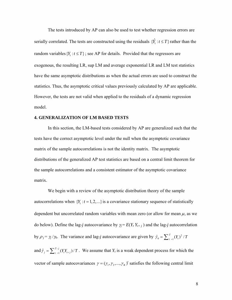
The tests introduced by AP can also be used to test whether regression errors are

serially correlated. The tests are constructed using the residuals ˆ{ : }tY t T≤ rather than the

random variables{ : }tY t T≤ ; see AP for details. Provided that the regressors are

exogenous, the resulting LR, sup LM and average exponential LR and LM test statistics

have the same asymptotic distributions as when the actual errors are used to construct the

statistics. Thus, the asymptotic critical values previously calculated by AP are applicable.

However, the tests are not valid when applied to the residuals of a dynamic regression

model.

4. GENERALIZATION OF LM BASED TESTS

In this section, the LM-based tests considered by AP are generalized such that the

tests have the correct asymptotic level under the null when the asymptotic covariance

matrix of the sample autocorrelations is not the identity matrix. The asymptotic

distributions of the generalized AP test statistics are based on a central limit theorem for

the sample autocorrelations and a consistent estimator of the asymptotic covariance

matrix.

We begin with a review of the asymptotic distribution theory of the sample

autocorrelations when { : 1,2,...}tY t = is a covariance stationary sequence of statistically

dependent but uncorrelated random variables with mean zero (or allow for mean μ, as we

do below). Define the lag-j autocovariance by γj = E(Yt Yt+ j ) and the lag-j autocorrelation

by ρ j = γj /γ0. The variance and lag-j autocovariance are given by 20 1

ˆ ( ) /Ttt

Y Tγ=

= ∑

and -

1ˆ ( ) /T j

j t t jtY Y Tγ +=

= ∑ . We assume that Yt is a weak dependent process for which the

vector of sample autocovariances 1 2( , ,..., )Kγ γ γ γ ′= satisfies the following central limit

9

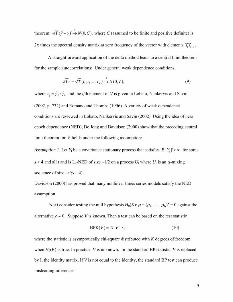
theorem: ˆ( ) (0, ),d

T N Cγ γ ′− → where C (assumed to be finite and positive definite) is

2π times the spectral density matrix at zero frequency of the vector with elements t t jYY − .

A straightforward application of the delta method leads to a central limit theorem

for the sample autocorrelations: Under general weak dependence conditions,

1 2( , ,..., ) (0, ),d

KT r T r r r N V′= → (9) where 0ˆ ˆ/j jr γ γ= and the ijth element of V is given in Lobato, Nankervis and Savin

(2002, p. 732) and Romano and Thombs (1996). A variety of weak dependence

conditions are reviewed in Lobato, Nankervis and Savin (2002). Using the idea of near

epoch dependence (NED), De Jong and Davidson (2000) show that the preceding central

limit theorem for γ̂ holds under the following assumption:

Assumption 1. Let Yt be a covariance stationary process that satisfies | |stE Y < ∞ for some

s > 4 and all t and is L2-NED of size –1/2 on a process Ut where Ut is an α-mixing

sequence of size –s/(s – 4).

Davidson (2000) has proved that many nonlinear times series models satisfy the NED

assumption.

Next consider testing the null hypothesis H0(K): ρ = (ρ1, … , ρK)’ = 0 against the

alternative ρ ≠ 0. Suppose V is known. Then a test can be based on the test statistic

1BPK( ) 'V Tr V r−= , (10)

where the statistic is asymptotically chi-square distributed with K degrees of freedom

when H0(K) is true. In practice, V is unknown. In the standard BP statistic, V is replaced

by I, the identity matrix. If V is not equal to the identity, the standard BP test can produce

misleading inferences.

10

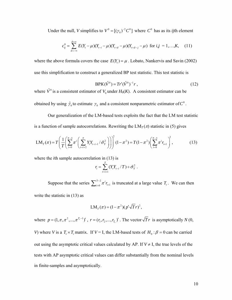
Under the null, V simplifies to 0 2 00[( ) ]V Cγ −= where 0C has as its ijth element

0 ( )( )( )( )d

ij t t i t d t d jd

c E Y Y Y Yμ μ μ μ=∞

− + + −=−∞

= − − − −∑ for i,j = 1,…,K, (11)

where the above formula covers the case ( )tE Y μ= . Lobato, Nankervis and Savin (2002)

use this simplification to construct a generalized BP test statistic. This test statistic is

0 0 1ˆ ˆBP ( ) ( )K V Tr V r−′= , (12) where 0V̂ is a consistent estimator of 0V under H0(K). A consistent estimator can be

obtained by using 0γ̂ to estimate 0γ and a consistent nonparametric estimator of 0C .

Our generalization of the LM-based tests exploits the fact that the LM test statistic

is a function of sample autocorrelations. Rewriting the LMT (π) statistic in (5) gives

2 22 2

2 2 21 1

0 2 0

1LM ( ) / (1 ) (1 ) ,T T T

i iT t t i Y i

i t i iT YY T r

Tπ π σ π π π

− −

− − += = + =

⎛ ⎞⎛ ⎞⎛ ⎞ ⎛ ⎞= − = −⎜ ⎟⎜ ⎟⎜ ⎟ ⎜ ⎟⎜ ⎟⎝ ⎠ ⎝ ⎠⎝ ⎠⎝ ⎠∑ ∑ ∑ (13)

where the ith sample autocorrelation in (13) is

2

1

( / )T

i t t i Yt i

r Y Y T σ−= +

= ÷∑ .

Suppose that the series 2

10

T iii

rπ−

+=∑ is truncated at a large value rT . We can then

write the statistic in (13) as

2 2LM ( ) (1 )( ) ,T p T rπ π ′= −

where 12(1, , ,..., )rTp π π π − ′= , 1 2( , ,..., )rTr r r r ′= . The vector T r is asymptotically N (0,

V) where V is a r rT T× matrix. If V = I, the LM-based tests of 0 : 0H β = can be carried

out using the asymptotic critical values calculated by AP. If V ≠ I, the true levels of the

tests with AP asymptotic critical values can differ substantially from the nominal levels

in finite-samples and asymptotically.

11

The level distortion of the LM-based tests when V ≠ I can be corrected

asymptotically by using T Lr in place of T r in (13) where 1V L L− ′= . Our proposed

generalization is to replace V by 0V and consistently estimate 0V by 0V̂ . The generalized

tests we consider are:

0

0 00

0 0

ˆsup LM ( , )ˆ ˆExp-LM ( ) LM ( , ) ( ),

1ˆ ˆExp-LM ( ) ln exp LM ( , ) ( ),2

T

T T

T T

V

V V dJ

V V dJ

π π

π π

π π

∈Π

∞

=

⎛ ⎞= ⎜ ⎟⎝ ⎠

∫

∫

(14)

where 0 2 0 2ˆ ˆLM ( , ) (1 )( )T V p T L rπ π ′= − with 0 1 0 0ˆ ˆ ˆ( )V L L− ′= . `

A brief sketch of proof that the generalized AP tests have the same limiting

distribution as the AP tests is the following. In the AP case where ( )Var T r = I, we have

that

22(1 ) ' (1 ) (0,1) (0,1),rd TT p r N Nπ π− ⎯⎯→ − =

when max(π) = 0.8 and rT = 20 ( 401 0.8 0.9999− = ), the parameter values used in our

numerical calculations. The asymptotic correlation between

2(1 )k kT p rπ ′− and 2(1 )m mT p rπ ′− is 2 2(1 )(1 )(1 ) /(1 )r rT Tk m k m k mπ π π π π π− − − − ,

where 12 3(1 ... ).rTj j j j jp π π π π −′ = Thus, the AP tests are functions of correlated

asymptotically standard normal variables, 2(1 )j jT p rπ ′− . In the case where ( )Var T r =

V we have that

2 0̂(1 ) (0,1),dT p L r Nπ ′− ⎯⎯→

12

and that the asymptotic correlation between 2 0̂(1 )k kT p L rπ ′− and 2 0̂(1 )m mT p L rπ ′− is

2 2(1 )(1 )(1 ) /(1 ).r rT Tk m k m k mπ π π π π π− − − − This shows that the generalized AP tests are the

same functions of asymptotically standard normal variables with identical asymptotic

correlations.

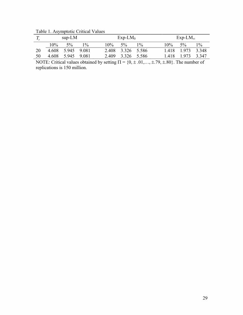
The asymptotic critical values reported by AP remain valid for our generalization

of the LM-based tests. We use critical values based on rT = 20, whereas AP use rT = 50.

We have set, as AP did, max |π| = 0.8. Using rT = 20 rather than 50 has a negligible

effect on the 1%, 5% and 10% asymptotic critical values through terms 2 1(1 )rTπ × −− . This

is seen in Table 1 where we report the asymptotic critical values for the three test

statistics for Π = {0, ± .01,…, ±.79, ±.80}, rT = 20 and rT = 50, using 150 million

replications.

The generalized versions of BP and LM-based tests require a consistent estimator

of 0V . We use the VARHAC estimation procedure proposed by den Haan and Levin

(1997). The consistency of the VARHAC estimator is proved by den Haan and Levin

(1998) under very general conditions. They demonstrate that, in many cases, the

VARHAC estimator achieves a faster convergence rate than kernel-based methods.

Francq et al. (2005, p. 539) also prove the consistency of the VARHAC estimator. Their

proof uses the existence of the eighth moment of tY and a mixing condition.

The VARHAC procedure uses a vector autoregressive (VAR) estimator of the

covariance matrix where the order of equation in the VAR is automatically selected. To

present the explicit formula for the VARHAC estimator of 0C , let ˆ ( )( )it t t iw Y Y Y Y−= − − ,

1 ,ˆ ˆ ˆ( ,..., ) 'rt t T tw w w= , and let S be the maximum lag order chosen for the VAR. For

13

consistency, den Haan and Levin (1998) also require that the maximum lag grows at rate

1/3T . The estimated residuals from the VAR regressions are

1

ˆˆ ˆ ˆS

t t s t ss

e w A w −=

= − ∑ ,

where ˆsA are the matrices of estimated coefficients from the VAR, and the estimated

innovation covariance matrix is

1

ˆ ˆ 'T

t tt S

e e T= +

Σ = ∑ .

Then the VARHAC estimator of 0C is

0 1 1

1 1

ˆ ˆ ˆ( ) ( ' )S S

s ss s

C I A I A− −

= =

= − Σ −∑ ∑ . (15)

We report results for the VAR with the AIC (Akaike (1973)) and the SBC

(Schwarz (1978)) criteria. The resulting estimators are denoted by ˆ (AIC)V and ˆ (SBC)V .

The maximum lag length is 3, 4, 5 and 8 for sample sizes T = 200, 500, 1000 and 5000,

and, for any equation in the VAR, the same lag length is used for each element of the

vector process. To mitigate the effect of occasional extreme estimates we used the

procedure of Andrews and Monahan (1992), and set the minimum singular values of the

inverse of the recoloring matrix, 1

ˆ ,S

ss

I A=

′− ∑ to be 0.005.

The form of the 0V matrix is simplified when the time series is a martingale

difference sequence. For a MDS process, the only possible nonzero elements of 0C are

terms of the form 2( ) ( )( )t t i t jE Y Y Yμ μ μ− −− − − . In (11) these occur at d = 0. Guo and

Phillips (1998) have developed a version of the BP test for the MDS case. This special

14

form of 0V matrix can also be used in constructing a generalization of the LM- based tests

for general MDS processes.

For certain MDS processes, such as Gaussian GARCH processes, 0V is diagonal,

with the jth diagonal element equal to 2 2 2( (0)) ( ) ( )t t jE Y Yγ μ μ−−− − . Generalizations of

the LM-based tests can be constructed for the diagonal case. The BP test for the diagonal

case has been repeatedly reinvented in the literature; see, for example, Taylor (1984),

Diebold (1986), Lo and MacKinlay (1989), Lobato, Nankervis and Savin (2001) and also

Deo (2000).

We denote the estimator of 0V in the general MDS case by GPV . A consistent

estimator of the ijth element of GPV is

2 20

1

ˆˆ ˆ ˆ/ and ( ) ( )( ) / ; , 1,...,r

TGP GP GPij ij ij t t i t j r

t T

v c c Y Y Y Y Y Y T i j Tγ − −= +

= = − − − =∑ . (16)

The diagonal 0V matrix is denoted by *V . A consistent estimator of the jth diagonal

element of *V is

* * 2 * 2 20 1

ˆˆ ˆ ˆ/ and ( ) ( ) / , 1,...,r

Tjj jj jj t t j rt T

v c c Y Y Y Y T j Tγ −= += = − − =∑ . (17)

As noted earlier, AP show that their tests apply to residuals from regressions with

exogenous regressors (Assumptions 4 and 5 in AP). The same holds for the generalized

tests. The reason these assumptions rule out an extension to dynamic regression models is

because they require that the conditional mean of the unobserved errors is zero given past

values of the errors and past and future values of the regressors.

5. MONTE CARLO COMPARISONS This section considers the true levels of the LM-based tests, the BP tests and the

Deo (2000) test when the tests use asymptotic critical values. The LM-based tests are the

15

sup LM, Exp-LM0 and Exp-LM∞ tests. The finite sample level-corrected powers of these

tests and the other tests are compared. The BP tests are included because they are widely

employed in the economics and finance literature and the Deo (2000) test is included

because it is consistent against all non-white noise alternatives when V is diagonal in the

MDS case, a property not shared by the BP tests.

The model we consider in the level experiments is the location model with

serially uncorrelated but dependent errors,

for 1,2,..., ,t tY t Tμ ε= + = (18)

where V ≠ I. The models used for the errors εt in the experiments include two MDS

processes and two non-MDS processes.

The two MDS models for the errors are variants of the GARCH model of

Bollerslev (1986), namely, Gaussian GARCH (1, 1) and the exponential GARCH (1, 1)

or EGARCH (1, 1). Both models are described in Campbell, Lo and MacKinlay (1997).

GARCH (1, 1). ,t t tZε σ= ⋅ where {Zt }is an iid N(0,1) sequence and

2 2 20 1 0 1t t tσ ω α ε β σ− −= + + . The constants α0 and β0 are such that 0 0 1α β+ < . This condition

is needed so that Yt is covariance stationary. He and Teräsvirta (1999) show that the

unconditional 2mth moment of Yt for GARCH (1, 1) models of Yt exists if and only if

20 0( ) 1m

tE Zα β+ < . We set ω = 0.001, α 0 = 0.08, and β0 = 0.89. With this parameter

setting, the He and Teräsvirta condition for the existence of the fourth and eighth

moments of Yt are satisfied. For this process, 20 ( ) 0.033,tE Yγ μ= − =

3 3/ 20( ) / 0,tE Y μ γ− = 4 4

0( ) / 3.83,tE Y μ γ− = and V is diagonal. We note that our results

16

are invariant to the value of ω. Estimates from stock return data suggest that 0 0α β+ is

close to one with β0 also close to one; for example, see Bera and Higgins (1997).

EGARCH (1, 1). ,t t tZε σ= ⋅ where {Zt }is an iid N(0,1) sequence and where

2 21 0 1 0 1ln( ) | | ln( )t t t tZ Zσ ω ψ α β σ− − −= + + + . We set ω = 0.01, 0.5ψ = ,α 0 = −0.2, and

β0 = 0.95. He, Teräsvirta and Malmsten (2002) show that Yt is stationary if | | 1β < and

that with Gaussian {Zt} all moments of Yt exist. We have that (the skewness is an

estimate) 20 ( ) 10.8tE Yγ μ= − = , 3 3/ 2

0( ) / 0,tE Y μ γ− = and 4 40( ) / 23.4,tE Y μ γ− = and V is

no longer diagonal. Our results are invariant to the value of the intercept and the

variance.

The two models for the non-MDS errors are the nonlinear moving average model,

and the bilinear model. Tong (1990) considers the nonlinear moving average model, and

Granger and Andersen (1978) the bilinear model. The motivation for entertaining non-

MDS processes is the growing evidence that the MDS assumption is too restrictive for

financial data; see, for example, El Babsiri and Zakoian (2001). For both models

considered below, V is non-diagonal.

Nonlinear Moving Average Model. Let εt = Zt -1⋅ Zt -2 ⋅ ( Zt -2 + Zt + c) where { Zt } is a

sequence of iid N(0, 1) random variables and c = 1.0. For this process all moments exist

with 2 3 3/ 2 4 40 0( ) 5, ( ) / 0, ( ) / 37.80.t t tE Y E Y E Yμ μ γ μ γ− = − = − =

Bilinear Model. Let εt = Zt + b⋅ Zt -1⋅ εt -2, where { Zt } is a sequence of iid N(0, σ2)

random variables, b = 0.50 and σ2 = 1.0. The Yt process is covariance stationary provided

that b2 σ2 < 1. The fourth moment of this process exists if 3b4σ4 < 1. For this process,

2 2 2 2( ) (1 )tE Y bμ σ σ− = − = 1.333, 3 3/ 20( ) / 0,tE Y μ γ− = and 4 4

0( ) /tE Y μ γ−

17

4 4 4 43(1 ) /(1 3 ) 3.462b bσ σ= − − = . Bera and Higgins (1997) have fitted a bilinear model

to stock return data.

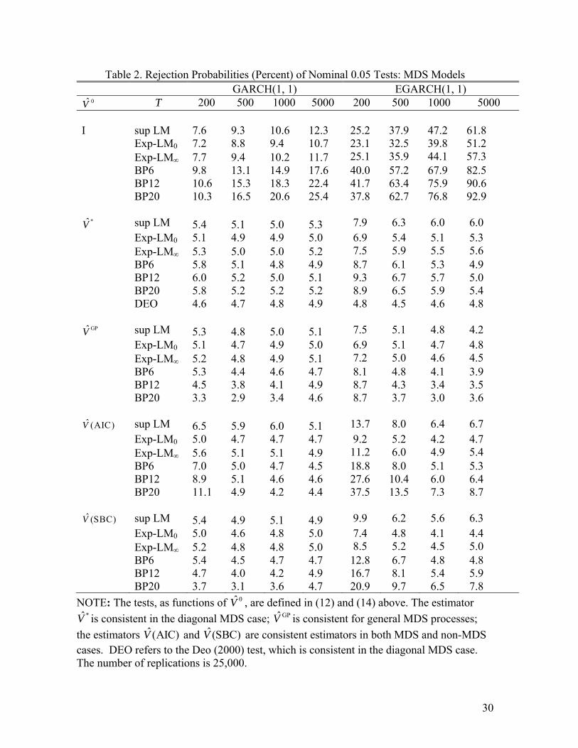
We simulated the finite-sample rejection probabilities (percent) of the nominal .05

LM, Exp-LM0 and Exp-LM∞ tests of 0 : 0H β = for the MDS and non-MDS error

models. The rejection probabilities for the sup LM, Exp-LM0 and Exp-LM∞ tests are

computed using { .80, .79,...,.79,.80}Π = − − , which is the same set as used by AP. The

rejection probabilities are based on rT = 20. Increasing rT does not produce a noticeable

difference in the rejection probabilities when using Π as defined above. For comparison,

the simulations included the BP6, BP12, BP20 tests and the Deo (2000) test; BP6 and

BP12 were considered by AP. The MDS and non-MDS models are simulated for sample

sizes T = 200, 500, 1000 and 5000 using 25, 000 replications. Results for the non-MDS

models are not reported because they do not change the conclusions from the MDS

models and also to save space.

The results for the GARCH models are presented in Table 2. The results show

that the differences between the true and nominal levels are substantial when the identity

matrix is used. The differences are largest for the BP tests with the EGARCH (1, 1)

model. The differences tend to increase as the sample size increases. The increase is large

for the EGARCH (1, 1).

Next we consider the generalized tests in Table 2. We first compare the LM –

based tests. The differences between the true and nominal levels tend to be essentially

eliminated for GARCH (1, 1) when the tests use the consistent estimators *V̂ , GPV̂ or

ˆ(SBC)V and T ≥ 500. For EGARCH (1, 1), the difference is essentially eliminated when

18

the tests use the consistent estimators GPV̂ or ˆ(SBC)V and T ≥ 500. In both cases larger

sample sizes are needed to eliminate the difference when ˆ(AIC)V is used, especially for

the sup LM test. Overall, the Exp-LM0 and Exp-LM∞ tests tend to have better control

over the level than the sup LM tests. The estimator of *V̂ is inconsistent in the EGARCH

case. The results for *V̂ in Table 2 show only a small tendency for over rejection at T =

1000 because the average off-diagonal elements of V are close to zero at this sample size.

Next consider other tests. The generalized BP tests generally tend to show less

satisfactory control over the level than the LM-based tests, especially BP20. The levels of

the Deo (2000) test are similar to those of the generalized LM tests in the V* case. We

also calculated the finite-sample rejection probabilities using the skewed t(5) GARCH (1,

1) using the standardized version given in Lambert and Laurent (2001) and the mixtures

of normal GARCH (1,1) proposed by Haas, Mittnik and Paolella, (2004). The previous

conclusions are not altered by the results for these latter models.

The location model (18) is also used for the power comparisons, but now with

serially correlated errors. Following AP, the models used for the errors εt include

1AR(1) : ,t t tuε φε −= +

1MA(1): ,t t tu uε θ −= +

6

1

7AR(6): ,6t t j t

j

j uε φ ε −=

−= +∑

12

1

13AR(12) : ,12t t j t

j

j uε φ ε −=

−= +∑

6

1

1

7AR(6) : ( 1) ,6

jt t j t

j

j uε φ ε+−

=

−± = − +∑

19

12

1

1

13AR(12) : ( 1) .12

jt t j t

j

j uε φ ε+−

=

−± = − +∑ (19)

The above models were chosen by AP because they include a wide variety of patterns of

serial correlation with both positive and negative serial correlations. The models used for

the innovations ut are the GARCH (1, 1) and EGARCH (1, 1) models and the nonlinear

moving average and bilinear models.

We calculated the .05 level-corrected powers by simulation for sample size T =

1000 using 25,000 replications. The finite-sample critical values are simulated using

25,000 replications. The parameter values are chosen so that the maximum powers are

approximately .4 and .8 for the two parameter values considered. All models are

simulated with an approximately stationary startup by taking the last T random variables

from a simulated sequence of the T + 500 random variables where startup values are set

equal to zero.

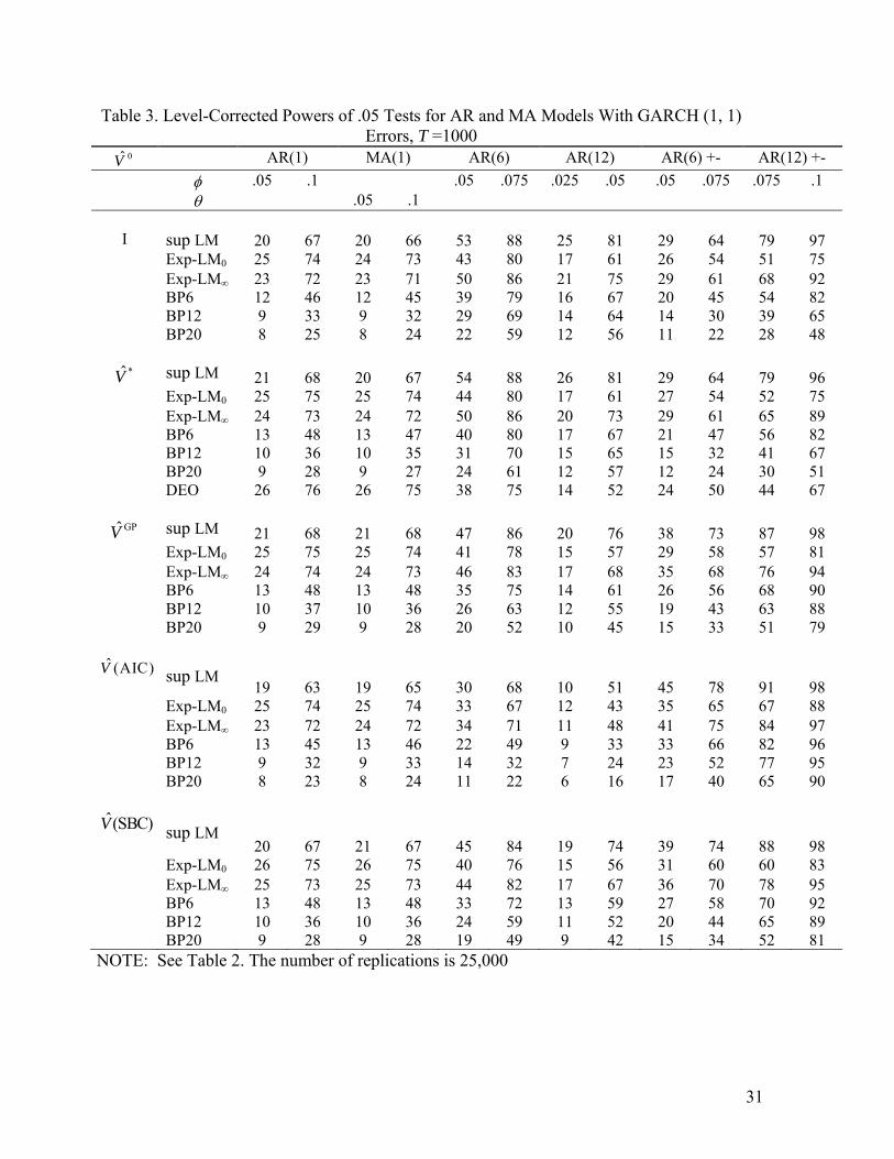
Table 3 presents the .05 level-corrected power of each of the tests for the AR(1),

MA(1), AR(6), AR(12), AR(6)± , and AR(12)± models with GARCH(1 ,1) innovations.

The powers in Table 3 present a mixed picture. A comparison of the LM-based tests

shows that Exp-LM0 tends to have the highest power for the AR(1) and MA(1) models

and the lowest power for the AR(12), AR(6)± , and AR(12)± models. For the latter

models, the sup LM test has the highest power. We conclude that the sup LM test has

higher all-around power than the Exp-LM∞ by a small margin. The same pattern tends to

hold when different values of φ and θ are used in the error models.

Among the BP tests, the BP6 has the highest power. The sup LM test has higher

power than the BP6 test and by a considerable margin in many cases. The powers of the

20

BP6 test tend to be higher than the powers of the Exp-LM0 for the AR(12)± model. The

powers of the BP6 test are lower than the powers of the Exp-LM∞ test. The power of the

Deo (2000) test is slightly higher than the power of the generalized AP tests in the AR(1)

and MA(1) cases, but in other cases it is smaller and sometimes substantially so.

When the powers of the tests are compared for models with EGARCH (1, 1)

innovations, our conclusions are essentially the same as those for GARCH (1, 1), and

similarly for the models with nonlinear moving average innovations and with bilinear

innovations.

Following AP, we also investigated the .05 level-corrected powers where ARMA

(1, 1) models are used for the errors. As previously, the innovations ut are generated by

the MDS or non-MDS models considered previously. In simulation experiments where

ARMA(1,1) models are used for the errors, the sup LM tests no longer have the best all

around power compared to the Exp-LM0 and Exp-LM∞ tests. Once the results from

ARMA error models are taken into account, the sup LM, Exp-LM0 and Exp-LM∞ tests

all have better power than the BP tests, but none is dominant.

Of course, the power results are influenced by the models and parameter values

used in the simulation experiments. Note that the data generation processes used in the

above experiments have declining weights as the lag length increases. As a consequence,

the first autocorrelation is dominant. This type of design is relevant for applications in

economics and finance. As we have seen, for this type the generalized AP tests tend to

have higher power than the generalized BP tests. However, the reverse can be hold for

designs where the first autocorrelation is not important. A simple example of a data

21

generation process with this property is an AR(2) where the coefficient on 1tY − is zero

and on 2tY − is negative. This caveat should be kept in mind when interpreting the results.

AP considered seasonal MA models for the errors εt. The models are

MA( ) : , 1,...,6.t t t jj u u jε θ −= + = (20) We calculated the .05 level corrected power for these error models with θ =.15 where the

ut are generated by the EGARCH (1, 1) model. For the seasonal models, the BP6 and

B12 tests are best of those considered, with BP6 test having the highest all around power.

This conclusion is the same as that reached by AP.

AP implement the tests using rT = 50 and we do so using rT = 20. We

investigated whether this affects the consistency of the tests. We found that with | Π | ≤

0.8 and a process with 1 20 21... 0, 0ρ ρ ρ= = = ≠ increasing the truncation lag does not

make any very noticeable difference to powers and thus the consistency of the tests as the

sample size T increases to 15,000. Further, we simulated the level-corrected powers for T

= 1000 using rT = 40. The powers of the LM-based tests for rT = 40 are essentially the

same for rT = 20, and hence the conclusions from the power comparisons are unchanged.

Computing. The random number generator used in the experiments was the very long

period generator RANLUX with luxury level p = 3; See Hamilton and James (1997). The

program used for VARHAC was the version of the program by den Haan and Levin

(http://econ.ucsd.edu/~wdenhaan/varhac.html) modified to run substantially faster.

6. EMPIRICAL APPLICATION As Campbell, Lo and MacKinlay (1997) note, the predictability of stock returns is

an active research topic. They illustrate the empirical relevance of predictability by

22

applying the BP tests to CRSP stock return indexes. In this section, their empirical

application is extended in two ways: First, results are presented for the AP tests as well as

the generalized AP and BP tests; second, results are presented for an extension of their

sample period.

Campbell, Lo and MacKinlay (1997) report the means, standard deviations, the

first four sample autocorrelations (in percent) as well as the BP5 and BP10 statistics in

their Table 2.4 for monthly, weekly and daily value-weighted (VWRETD) and equal-

weighted (EWRETD) stock return indexes (NYSE/AMEX). The sample period is July 3,

1962 to December 31, 1994. We replicated the results by Campbell, Lo and MacKinlay

(1997) for this sample period and the sub-periods they selected.

In this section, the sample period is July 3, 1962 to December 30, 2005. Results

were calculated for the sup LM, Exp-LM0 and Exp-LM∞ tests, and the generalized AP

and BP tests, both for the sample period and sub-periods considered by Campbell Lo and

MacKinlay (1997) and for the extended sample period and selected sub-periods. The

skewness and kurtosis statistics were also calculated to provide a check on the normality

of the returns. As expected, the kurtosis statistics provide strong evidence against

normality.

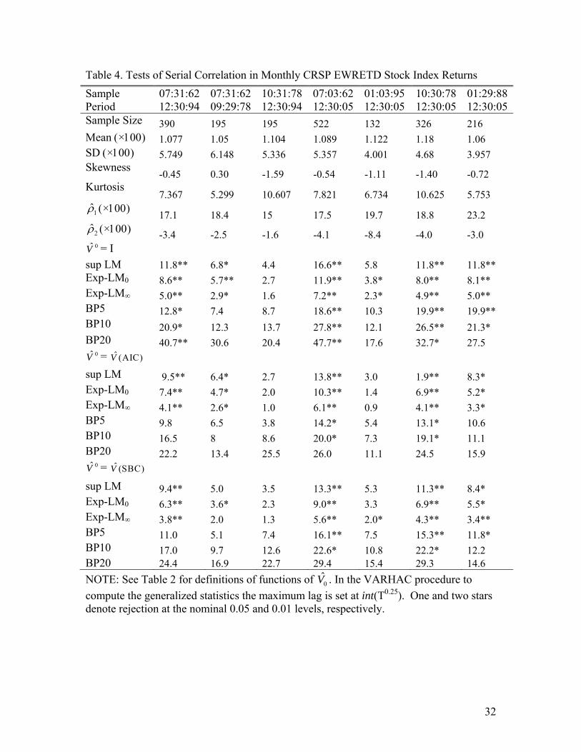
For the sake of brevity, we only report results for the monthly equal-weighted

stock return indexes. Table 4 illustrates that inferences from the generalized AP tests can

conflict with those from the generalized BP tests. The generalized AP tests tend to reject

and the generalized BP tests tend not to reject. For the data used by Campbell, Lo and

MacKinlay (1997), the BP tests tend to not reject at the nominal .05 level and similarly

for the generalized BP tests. The greater number of rejections by the generalized AP tests

23

may be explained by the higher power of the generalized AP tests compared to the

generalized BP tests.

Table 4 also shows that both the AP and BP tests tend to reject at the nominal .05

and or .01 levels for the extended sample period and selected sub-periods. The same is

true for the generalized AP tests. Again there are substantially fewer rejections by the

generalized BP tests than the generalized AP tests.

In light of our Monte Carlo experiments, the results reported by Campbell, Lo

and MacKinlay (1997) for the BP tests are difficult to interpret in isolation. Although the

BP statistics are often enormous for weekly and daily data, this alone does not provide

strong evidence that the null of zero correlation is false. This is because the BP tests tend

to substantially over-reject when data are generated by uncorrelated dependent processes

such as a GARCH (1, 1) or EGARCH (1, 1) model. In particular, the over-rejection is

most pronounced for large sample sizes, sizes similar to those in this empirical

application.

The motivation of the empirical application is predictability of stock returns,

which is characterized by a MDS condition in stock returns. The MDS hypothesis implies

that stock returns are white noises, so it is valid to use tests for serial correlation in testing

the predictability of stock returns. Hence, robustness under conditional heteroskedasticity

in the case of GARCH and EGARCH is an appealing property of the generalized AP test.

However, robustness under the non-MDS cases (nonlinear MA and bilinear) may be

interpreted as a drawback for this purpose because non-MDS processes which can be

used for prediction will be missed.

7. CONCLUDING COMMENTS

24

In the simulations in this paper, the differences between the true and nominal

levels of the generalized AP tests are essentially zero for suitable sample sizes, and the

generalized AP tests have good power properties for nonseasonal alternatives compared

to the generalized Box-Pierce tests and the Deo (2000) tests. The Exp-LM∞ test is

recommended for nonseasonal applications in economics and finance. The paper includes

an empirical application to stock return indexes that is motivated by the search for

predictability in returns. The results illustrate that inferences from the generalized AP

tests can conflict with those from the generalized Box-Pierce tests and can make a

difference to the inferences drawn from the data.

Andrews, Liu and Ploberger (1998) extended their approach to testing white noise

against multiplicative seasonal ARMA (1, 1) models. A topic for further research would

be to use our approach to generalize the LM-based test for this case. The generalized

LM-based tests do not apply to residuals from ARMA models. We plan to investigate this

topic in future research.

ACKNOWLEDGEMENTS The authors gratefully acknowledge the helpful comments of the editor and referees. Don

Andrews, John Geweke and Ignacio Lobato provided useful advice.

REFERENCES Akaike, H. (1973), “Information Theory and the Extension of Maximum Likelihood

Principle,” in Second International Symposium on Information Theory, eds. B.

Petrov and F.Casaki, Budapest: Akailseoniai-Kiudo, pp. 267-281.

Andrews, B., Davis, R. A. and Breidt, F. J. (2006), “Maximum Likelihood Estimation for

All-Pass Time Series Models,” Journal of Multivariate Analysis, 97, 1638-1659.

25

Andrews, D. W. K., and Monahan, J. C. (1992), “An Improved Heteroskedasticity and

Autocorrelation Consistent Covariance Matrix Estimator,” Econometrica, 60,

953-966.

Andrews, D.W. K., and Ploberger, W. (1994), “Optimal Tests When a Nuisance

Parameter Is Present Only Under the Alternative,” Econometrica, 62, 1383-1414.

Andrews, D.W. K., and Ploberger, W. (1995), “Admissibility of the Likelihood Ratio

Test When a Nuisance Parameter Is Present Only Under the Alternative,”

Annals of Statistics, 23, 1609-1609.

Andrews, D.W. K., and Ploberger, W. (1996), “Testing for Serial Correlation Against an

ARMA (1, 1) Process,” Journal of the American Statistical Association, 91, 1331

1342.

Andrews, D.W. K., Liu, X., and Ploberger, W. (1998), “Tests for White Noise Against

Alternatives With Both Seasonal and Nonseasonal Serial Correlation,”

Biometrika, 85, 727-740.

Bera, A.K., and Higgins, M. L. (1997), “ARCH and Bilinearity As Competing Models

For Nonlinear Dependence,” Journal of Business and Economic Statistics,” 15,

43-51.

Bollerslev, T. (1986), “Generalized Autoregressive Conditional Heteroskedasticity,”

Journal of Econometrics, 31, 307-327.

Box, G.E.P., and Pierce, D. A. (1970), “Distribution of Residual Autocorrelations in

Autoregressive Integrated Moving Average Time Series Models,” Journal of the

American Statistical Association, 93, 1509-1526.

Campbell, J.Y., Lo, A. W., and MacKinlay, A. C., (1997), The Econometrics of Financial

Markets, New Jersey: Princeton University Press.

26

Chen, W. W. and Deo, R. S., (2004), “A General Portmanteau Goodness-of-Fit Test for

Time Series Models,” Econometric Theory, 20, 382-416.

Davidson, J. (2000), “When is a Time Series I(0)? Evaluating the Memory Properties of

Nonlinear Dynamic Models,” Preprint, Cardiff University.

De Jong, R. M., and Davidson, J. (2000), “The Functional Central Limit Theorem and

Weak Convergence to Stochastic Integrals, Part 1: Weakly Dependent Processes,”

Econometric Theory, 16, 621-642.

Den Haan, W.J., and Levin, A. (1997), “A Practitioner’s Guide to Robust Covariance

Matrix Estimation,” in Handbook of Statistics: Robust Inference, eds. G. S.

Maddala and C.R. Rao, Amsterdam: North-Holland, pp.191-341.

Den Haan, W.J., and Levin, A. (1998), “Vector Autoregressive Covariance Matrix

Estimation,” Manuscript, Department of Economics, San Diego: University of

California.

Deo, R. S. (2000), “Spectral Tests of the Martingale Hypothesis Under Conditional

Heteroskedasticity,” Journal of Econometrics, 99, 291-315.

Diebold, F. X. (1986), “Testing for Serial Correlation in the Presence of

Heteroskedasticity,” Proceedings of the American Statistical Association,

Business and Economics Statistics Section, 323-328.

Durlauf, S. (1991), “Spectral Based Testing for the Martingale Hypothesis,” Journal of

Econometrics,” 50, 1-19.

El Babsiri, M., and Zakoian, J.-M. (2001), “Contemporaneous Asymmetry in GARCH

Processes,” Journal of Econometrics, 101, 257-294.

Francq, C., Roy, R., and Zakoian, J.-M. (2005), “Diagnostic Checking in ARMA Models

27

with Uncorrelated Errors,” Journal of the American Statistical Association, 100,

532-544.

Granger, C. W. J., and Andersen, A. P. (1978), An Introduction to Bilinear Time Series

Models, Gottingen: Vanenhoek and Ruprecht.

Guo, B. B., and Phillips, P.C. B. (1998), “Testing for Autocorrelation and Unit Roots in

the Presence of Conditional Heteroskedasticity of Unknown Form,” Manuscript,

Cowles Foundation for Research in Economics, New Haven: Yale University.

Hamilton, K.G., and James, F. (1997), “Acceleration of RANLUX,” Computer Physics

Communications, 101, 241-248.

Haas, M., Mittnik, S., and Paolella, M. (2004), “Mixed Normal Conditional

Heteroskedasticity,” Journal of Financial Econometrics, 2, 211–250.

He, C., and Teräsvirta, T. (1999), “Properties of Moments of a Family of GARCH

Processes,” Journal of Econometrics, 92, 173 -192.

He, C., Teräsvirta, T., and Malmsten, H. (2002), “Moment Structure of a Family of First-

Order Exponential GARCH models,” Econometric Theory, 18, 868-885.

Hong, Y. (1996), “Consistent Testing for Serial Correlation of Unknown Form,”

Econometrica, 64, 837-864.

Hong, Y. and Lee, Y. J., (2003), “Consistent Testing for Serial Correlation of Unknown

Form Under General Conditional Heteroskedasticity,” Technical Report,

Departments of Economics and Statistical Sciences, Cornell University.

Lambert, P., and Laurent, S. (2001), “Modelling Financial Time Series Using GARCH-

Type Models With a Skewed Student Distribution for the Innovations,” Working

Paper, Universite Catholique de Louvain and Universite de Liege.

28

Lo, A.W., and MacKinlay, A.C. (1989), “The size and power of the variance ratio test in

finite samples: A Monte Carlo investigation”, Journal of Econometrics, 40, 203-

238.

Lobato, I., Nankervis, J. C., and Savin, N.E. (2001), “Testing for Autocorrelation Using a

Modified Box-Pierce Q Test,” International Economic Review, 42, 187-205.

Lobato, I., Nankervis, J. C., and Savin, N.E. (2002), “Testing for Zero Autocorrelation in

the Presence of Statistical Dependence,” Econometric Theory, 18, 730-743.

Poterba, J.M., and Summers, L.H. (1988), “Mean Reversion in Stock Prices: Evidence

and Implications,” Journal of Financial Economics, 22, 27-59.

Pötscher, B. M. (1990), “Estimation of Autoregressive Moving-Average Order Given an

Infinite Number of Models and Approximation of Spectral Densities,” Journal of

Time Series Analysis, 11, 165-179.

Romano, J.L., and Thombs, L.A. (1996), “Inference for Autocorrelations Under Weak

Assumptions,” Journal of American Statistical Association, 91, 590-600.

Schwartz, G. (1978), “Estimating the Dimension of a Model,” Annals of Statistics, 6,

461-464.

Taylor, S. (1984), “Estimating the Variances of Autocorrelations Calculated From

Financial Time Series,” Applied Statistics, 33, 300-308.

Taylor, S.J. (2005), Asset Price Dynamics, Volatility, and Prediction, Princeton:

Princeton University Press.

Tong, H. (1990), Nonlinear Time Series, Oxford: Oxford University Press.

29

Table 1. Asymptotic Critical Values rT sup-LM Exp-LM0 Exp-LM∞

10% 5% 1% 10% 5% 1% 10% 5% 1% 20 4.608 5.945 9.081 2.408 3.326 5.586 1.418 1.973 3.348 50 4.608 5.945 9.081 2.409 3.326 5.586 1.418 1.973 3.347 NOTE: Critical values obtained by setting Π = {0, ± .01,…, ±.79, ±.80}. The number of replications is 150 million.

30

Table 2. Rejection Probabilities (Percent) of Nominal 0.05 Tests: MDS Models GARCH(1, 1) EGARCH(1, 1)

0V̂ T 200 500 1000 5000 200 500 1000 5000 I sup LM 7.6 9.3 10.6 12.3 25.2 37.9 47.2 61.8 Exp-LM0 7.2 8.8 9.4 10.7 23.1 32.5 39.8 51.2 Exp-LM∞ 7.7 9.4 10.2 11.7 25.1 35.9 44.1 57.3 BP6 9.8 13.1 14.9 17.6 40.0 57.2 67.9 82.5 BP12 10.6 15.3 18.3 22.4 41.7 63.4 75.9 90.6 BP20 10.3 16.5 20.6 25.4 37.8 62.7 76.8 92.9

*V̂ sup LM 5.4 5.1 5.0 5.3 7.9 6.3 6.0 6.0 Exp-LM0 5.1 4.9 4.9 5.0 6.9 5.4 5.1 5.3 Exp-LM∞ 5.3 5.0 5.0 5.2 7.5 5.9 5.5 5.6 BP6 5.8 5.1 4.8 4.9 8.7 6.1 5.3 4.9 BP12 6.0 5.2 5.0 5.1 9.3 6.7 5.7 5.0 BP20 5.8 5.2 5.2 5.2 8.9 6.5 5.9 5.4 DEO 4.6 4.7 4.8 4.9 4.8 4.5 4.6 4.8

GPV̂ sup LM 5.3 4.8 5.0 5.1 7.5 5.1 4.8 4.2 Exp-LM0 5.1 4.7 4.9 5.0 6.9 5.1 4.7 4.8 Exp-LM∞ 5.2 4.8 4.9 5.1 7.2 5.0 4.6 4.5 BP6 5.3 4.4 4.6 4.7 8.1 4.8 4.1 3.9 BP12 4.5 3.8 4.1 4.9 8.7 4.3 3.4 3.5 BP20 3.3 2.9 3.4 4.6 8.7 3.7 3.0 3.6 ˆ (AIC)V sup LM 6.5 5.9 6.0 5.1 13.7 8.0 6.4 6.7

Exp-LM0 5.0 4.7 4.7 4.7 9.2 5.2 4.2 4.7 Exp-LM∞ 5.6 5.1 5.1 4.9 11.2 6.0 4.9 5.4 BP6 7.0 5.0 4.7 4.5 18.8 8.0 5.1 5.3 BP12 8.9 5.1 4.6 4.6 27.6 10.4 6.0 6.4 BP20 11.1 4.9 4.2 4.4 37.5 13.5 7.3 8.7 ˆ (SBC)V sup LM 5.4 4.9 5.1 4.9 9.9 6.2 5.6 6.3

Exp-LM0 5.0 4.6 4.8 5.0 7.4 4.8 4.1 4.4 Exp-LM∞ 5.2 4.8 4.8 5.0 8.5 5.2 4.5 5.0 BP6 5.4 4.5 4.7 4.7 12.8 6.7 4.8 4.8 BP12 4.7 4.0 4.2 4.9 16.7 8.1 5.4 5.9 BP20 3.7 3.1 3.6 4.7 20.9 9.7 6.5 7.8

NOTE: The tests, as functions of 0V̂ , are defined in (12) and (14) above. The estimator *V̂ is consistent in the diagonal MDS case; GPV̂ is consistent for general MDS processes;

the estimators ˆ(AIC)V and ˆ(SBC)V are consistent estimators in both MDS and non-MDS cases. DEO refers to the Deo (2000) test, which is consistent in the diagonal MDS case. The number of replications is 25,000.

31

Table 3. Level-Corrected Powers of .05 Tests for AR and MA Models With GARCH (1, 1) Errors, T =1000

0V̂ AR(1) MA(1) AR(6) AR(12) AR(6) +- AR(12) +- φ .05 .1 .05 .075 .025 .05 .05 .075 .075 .1 θ .05 .1 I sup LM 20 67 20 66 53 88 25 81 29 64 79 97 Exp-LM0 25 74 24 73 43 80 17 61 26 54 51 75 Exp-LM∞ 23 72 23 71 50 86 21 75 29 61 68 92 BP6 12 46 12 45 39 79 16 67 20 45 54 82 BP12 9 33 9 32 29 69 14 64 14 30 39 65 BP20 8 25 8 24 22 59 12 56 11 22 28 48 *V̂ sup LM 21 68 20 67 54 88 26 81 29 64 79 96 Exp-LM0 25 75 25 74 44 80 17 61 27 54 52 75 Exp-LM∞ 24 73 24 72 50 86 20 73 29 61 65 89 BP6 13 48 13 47 40 80 17 67 21 47 56 82 BP12 10 36 10 35 31 70 15 65 15 32 41 67 BP20 9 28 9 27 24 61 12 57 12 24 30 51 DEO 26 76 26 75 38 75 14 52 24 50 44 67 GPV̂ sup LM 21 68 21 68 47 86 20 76 38 73 87 98 Exp-LM0 25 75 25 74 41 78 15 57 29 58 57 81 Exp-LM∞ 24 74 24 73 46 83 17 68 35 68 76 94 BP6 13 48 13 48 35 75 14 61 26 56 68 90 BP12 10 37 10 36 26 63 12 55 19 43 63 88 BP20 9 29 9 28 20 52 10 45 15 33 51 79

ˆ (AIC)V

sup LM 19 63 19 65 30 68 10 51 45 78 91 98

Exp-LM0 25 74 25 74 33 67 12 43 35 65 67 88 Exp-LM∞ 23 72 24 72 34 71 11 48 41 75 84 97 BP6 13 45 13 46 22 49 9 33 33 66 82 96 BP12 9 32 9 33 14 32 7 24 23 52 77 95 BP20 8 23 8 24 11 22 6 16 17 40 65 90

ˆ(SBC)V

sup LM 20 67 21 67 45 84 19 74 39 74 88 98

Exp-LM0 26 75 26 75 40 76 15 56 31 60 60 83 Exp-LM∞ 25 73 25 73 44 82 17 67 36 70 78 95 BP6 13 48 13 48 33 72 13 59 27 58 70 92 BP12 10 36 10 36 24 59 11 52 20 44 65 89 BP20 9 28 9 28 19 49 9 42 15 34 52 81

NOTE: See Table 2. The number of replications is 25,000

32

Table 4. Tests of Serial Correlation in Monthly CRSP EWRETD Stock Index Returns

NOTE: See Table 2 for definitions of functions of 0̂V . In the VARHAC procedure to compute the generalized statistics the maximum lag is set at int(T0.25). One and two stars denote rejection at the nominal 0.05 and 0.01 levels, respectively.

Sample Period

07:31:62 12:30:94

07:31:62 09:29:78

10:31:7812:30:94

07:03:62 12:30:05

01:03:95 12:30:05

10:30:78 12:30:05

01:29:88 12:30:05

Sample Size 390 195 195 522 132 326 216 Mean (×100) 1.077 1.05 1.104 1.089 1.122 1.18 1.06 SD (×100) 5.749 6.148 5.336 5.357 4.001 4.68 3.957 Skewness -0.45 0.30 -1.59 -0.54 -1.11 -1.40 -0.72 Kurtosis

7.367 5.299 10.607 7.821 6.734 10.625 5.753 1ρ̂ (×100) 17.1 18.4 15 17.5 19.7 18.8 23.2 2ρ̂ (×100) -3.4 -2.5 -1.6 -4.1 -8.4 -4.0 -3.0 0V̂ = I

sup LM 11.8** 6.8* 4.4 16.6** 5.8 11.8** 11.8** Exp-LM0 8.6** 5.7** 2.7 11.9** 3.8* 8.0** 8.1** Exp-LM∞ 5.0** 2.9* 1.6 7.2** 2.3* 4.9** 5.0** BP5 12.8* 7.4 8.7 18.6** 10.3 19.9** 19.9** BP10 20.9* 12.3 13.7 27.8** 12.1 26.5** 21.3* BP20 40.7** 30.6 20.4 47.7** 17.6 32.7* 27.5

0V̂ = ˆ (AIC)V sup LM 9.5** 6.4* 2.7 13.8** 3.0 1.9** 8.3* Exp-LM0 7.4** 4.7* 2.0 10.3** 1.4 6.9** 5.2* Exp-LM∞ 4.1** 2.6* 1.0 6.1** 0.9 4.1** 3.3* BP5 9.8 6.5 3.8 14.2* 5.4 13.1* 10.6 BP10 16.5 8 8.6 20.0* 7.3 19.1* 11.1 BP20 22.2 13.4 25.5 26.0 11.1 24.5 15.9

0V̂ = ˆ (SBC)V sup LM 9.4** 5.0 3.5 13.3** 5.3 11.3** 8.4* Exp-LM0 6.3** 3.6* 2.3 9.0** 3.3 6.9** 5.5* Exp-LM∞ 3.8** 2.0 1.3 5.6** 2.0* 4.3** 3.4** BP5 11.0 5.1 7.4 16.1** 7.5 15.3** 11.8* BP10 17.0 9.7 12.6 22.6* 10.8 22.2* 12.2 BP20 24.4 16.9 22.7 29.4 15.4 29.3 14.6