An Econometric Model of

Serial Correlation and Illiquidity

In Hedge Fund Returns∗

Mila Getmansky, Andrew W. Lo, and Igor Makarov†

This Draft: April 28, 2003

Abstract

The returns to hedge funds and other alternative investments are often highly serially cor-related, in sharp contrast to the returns of more traditional investment vehicles such aslong-only equity portfolios and mutual funds. In this paper, we explore several sources ofsuch serial correlation and show that the most likely explanation is illiquidity exposure,i.e., investments in securities that are not actively traded and for which market prices arenot always readily available. For portfolios of illiquid securities, reported returns will tendto be smoother than true economic returns, which will understate volatility and increaserisk-adjusted performance measures such as the Sharpe ratio. We propose an economet-ric model of illiquidity exposure and develop estimators for the smoothing profile as wellas a smoothing-adjusted Sharpe ratio. For a sample of 908 hedge funds drawn from theTASS database, we show that our estimated smoothing coefficients vary considerably acrosshedge-fund style categories and may be a useful proxy for quantifying illiquidity exposure.

Keywords: Hedge Funds; Serial Correlation; Performance Smoothing; Liquidity; MarketEfficiency.

JEL Classification: G12

∗This research was supported by the MIT Laboratory for Financial Engineering. We thank Cliff Asness,David Geltner, Jacob Goldfield, Stephanie Hogue, Stephen Jupp, SP Kothari, Bob Merton, Myron Scholes,Bill Schwert, Jonathan Spring, Andre Stern, Svetlana Sussman, a referee, and seminar participants atHarvard, the MIT Finance Student Lunch Group, Morgan Stanley, and the 2001 Fall Q Group Conferencefor many stimulating discussions and comments.

†MIT Sloan School of Management. Corresponding author: Andrew W. Lo, MIT Sloan School, 50 Memo-rial Drive, E52-432, Cambridge, MA 02142–1347, (617) 253–0920 (voice), (617) 258–5727 (fax), alo@mit.edu(email).

Contents

1 Introduction 1

2 Literature Review 4

3 Other Sources of Serial Correlation 63.1 Time-Varying Expected Returns . . . . . . . . . . . . . . . . . . . . . . . . . 83.2 Time-Varying Leverage . . . . . . . . . . . . . . . . . . . . . . . . . . . . . . 123.3 Incentive Fees with High-Water Marks . . . . . . . . . . . . . . . . . . . . . 15

4 An Econometric Model of Smoothed Returns 184.1 Implications For Performance Statistics . . . . . . . . . . . . . . . . . . . . . 224.2 Examples of Smoothing Profiles . . . . . . . . . . . . . . . . . . . . . . . . . 25

5 Estimation of Smoothing Profiles and Sharpe Ratios 305.1 Maximum Likelihood Estimation . . . . . . . . . . . . . . . . . . . . . . . . 305.2 Linear Regression Analysis . . . . . . . . . . . . . . . . . . . . . . . . . . . . 325.3 Specification Checks . . . . . . . . . . . . . . . . . . . . . . . . . . . . . . . 355.4 Smoothing-Adjusted Sharpe Ratios . . . . . . . . . . . . . . . . . . . . . . . 37

6 Empirical Analysis 416.1 Summary Statistics . . . . . . . . . . . . . . . . . . . . . . . . . . . . . . . . 456.2 Smoothing Profile Estimates . . . . . . . . . . . . . . . . . . . . . . . . . . . 456.3 Cross-Sectional Regressions . . . . . . . . . . . . . . . . . . . . . . . . . . . 566.4 Illiquidity Vs. Smoothing . . . . . . . . . . . . . . . . . . . . . . . . . . . . . 626.5 Smoothing-Adjusted Sharpe Ratio Estimates . . . . . . . . . . . . . . . . . . 63

7 Conclusions 66

A Appendix 69A.1 Proof of Proposition 3 . . . . . . . . . . . . . . . . . . . . . . . . . . . . . . 69A.2 Proof of Proposition 4 . . . . . . . . . . . . . . . . . . . . . . . . . . . . . . 70A.3 Proof of Proposition 5 . . . . . . . . . . . . . . . . . . . . . . . . . . . . . . 75A.4 TASS Fund Category Definitions . . . . . . . . . . . . . . . . . . . . . . . . 75A.5 Supplementary Empirical Results . . . . . . . . . . . . . . . . . . . . . . . . 76

1 Introduction

One of the fastest growing sectors of the financial services industry is the hedge-fund or

“alternative investments” sector. Long the province of foundations, family offices, and high-

net-worth investors, hedge funds are now attracting major institutional investors such as

large state and corporate pension funds and university endowments, and efforts are underway

to make hedge-fund investments available to individual investors through more traditional

mutual-fund investment vehicles. One of the main reasons for such interest is the performance

characteristics of hedge funds—often known as “high-octane” investments, many hedge funds

have yielded double-digit returns to their investors and, in some cases, in a fashion that seems

uncorrelated with general market swings and with relatively low volatility. Most hedge

funds accomplish this by maintaining both long and short positions in securities—hence the

term “hedge” fund—which, in principle, gives investors an opportunity to profit from both

positive and negative information while, at the same time, providing some degree of “market

neutrality” because of the simultaneous long and short positions.

However, several recent empirical studies have challenged these characterizations of hedge-

fund returns, arguing that the standard methods of assessing their risks and rewards may

be misleading. For example, Asness, Krail and Liew (2001) show in some cases where hedge

funds purport to be market neutral, i.e., funds with relatively small market betas, including

both contemporaneous and lagged market returns as regressors and summing the coefficients

yields significantly higher market exposure. Moreover, in deriving statistical estimators for

Sharpe ratios of a sample of mutual and hedge funds, Lo (2002) shows that the correct

method for computing annual Sharpe ratios based on monthly means and standard devia-

tions can yield point estimates that differ from the naive Sharpe ratio estimator by as much

as 70%.

These empirical properties may have potentially significant implications for assessing the

risks and expected returns of hedge-fund investments, and can be traced to a single common

source: significant serial correlation in their returns.

This may come as some surprise because serial correlation is often (though incorrectly)

associated with market inefficiencies, implying a violation of the Random Walk Hypothe-

sis and the presence of predictability in returns. This seems inconsistent with the popular

belief that the hedge-fund industry attracts the best and the brightest fund managers in

the financial services sector. In particular, if a fund manager’s returns are predictable, the

implication is that the manager’s investment policy is not optimal; if his returns next month

can be reliably forecasted to be positive, he should increase his positions this month to take

advantage of this forecast, and vice versa for the opposite forecast. By taking advantage of

1

such predictability the fund manager will eventually eliminate it, along the lines of Samuel-

son’s (1965) original “proof that properly anticipated prices fluctuate randomly”. Given

the outsize financial incentives of hedge-fund managers to produce profitable investment

strategies, the existence of significant unexploited sources of predictability seems unlikely.

In this paper, we argue that in most cases, serial correlation in hedge-fund returns is not

due to unexploited profit opportunities, but is more likely the result of illiquid securities that

are contained in the fund, i.e., securities that are not actively traded and for which market

prices are not always readily available. In such cases, the reported returns of funds con-

taining illiquid securities will appear to be smoother than “true” economic returns—returns

that fully reflect all available market information concerning those securities—and this, in

turn, will impart a downward bias on the estimated return variance and yield positive serial

return correlation. The prospect of spurious serial correlation and biased sample moments

in reported returns is not new. Such effects have been derived and empirically documented

extensively in the literature on “nonsynchronous trading”, which refers to security prices

recorded at different times but which are erroneously treated as if they were recorded simul-

taneously.1 However, this literature has focused exclusively on equity market-microstructure

effects as the sources of nonsynchronicity—closing prices that are set at different times, or

prices that are “stale”—where the temporal displacement is on the order of minutes, hours,

or, in extreme cases, several days.2 In the context of hedge funds, we argue in this paper that

serial correlation is the outcome of illiquidity exposure, and while nonsynchronous trading

may be one symptom or by-product of illiquidity, it is not the only aspect of illiquidity that

affects hedge-fund returns. Even if prices were sampled synchronously, they may still yield

highly serially correlated returns if the securities are not actively traded.3 Therefore, al-

1 For example, the daily prices of financial securities quoted in the Wall Street Journal are usually“closing” prices, prices at which the last transaction in each of those securities occurred on the previousbusiness day. If the last transaction in security A occurs at 2:00pm and the last transaction in security Boccurs at 4:00pm, then included in B’s closing price is information not available when A’s closing price wasset. This can create spurious serial correlation in asset returns since economy-wide shocks will be reflectedfirst in the prices of the most frequently traded securities, with less frequently traded stocks responding witha lag. Even when there is no statistical relation between securities A and B, their reported returns willappear to be serially correlated and cross-correlated simply because we have mistakenly assumed that theyare measured simultaneously. One of the first to recognize the potential impact of nonsynchronous pricequotes was Fisher (1966). Since then more explicit models of non-trading have been developed by Atchison,Butler, and Simonds (1987), Dimson (1979), Cohen, Hawawini, et al. (1983a,b), Shanken (1987), Cohen,Maier, et al. (1978, 1979, 1986), Kadlec and Patterson (1999), Lo and MacKinlay (1988, 1990), and Scholesand Williams (1977). See Campbell, Lo, and MacKinlay (1997, Chapter 3) for a more detailed review of thisliterature.

2For such application, Lo and MacKinlay (1988, 1990) and Kadlec and Patterson (1999) show thatnonsynchronous trading cannot explain all of the serial correlation in weekly returns of equal- and value-weighted portfolios of US equities during the past three decades.

3In fact, for most hedge funds, returns computed on a monthly basis, hence the pricing or “mark-to-

2

though our formal econometric model of illiquidity is similar to those in the nonsynchronous

trading literature, the motivation is considerably broader—linear extrapolation of prices for

thinly traded securities, the use of smoothed broker-dealer quotes, trading restrictions aris-

ing from control positions and other regulatory requirements, and, in some cases, deliberate

performance-smoothing behavior—and the corresponding interpretations of the parameter

estimates must be modified accordingly.

Regardless of the particular mechanism by which hedge-fund returns are smoothed and

serial correlation is induced, the common theme and underlying driver is illiquidity expo-

sure, and although we argue that the sources of serial correlation are spurious for most hedge

funds, nevertheless, the economic impact of serial correlation can be quite real. For example,

spurious serial correlation yields misleading performance statistics such as volatility, Sharpe

ratio, correlation, and market beta estimates, statistics commonly used by investors to deter-

mine whether or not they will invest in a fund, how much capital to allocate to a fund, what

kinds of risk exposures they are bearing, and when to redeem their investments. Moreover,

spurious serial correlation can lead to wealth transfers between new, existing, and departing

investors, in much the same way that using stale prices for individual securities to compute

mutual-fund net-asset-values can lead to wealth transfers between buy-and-hold investors

and day-traders (see, for example, Boudoukh et al., 2002).

In this paper, we develop an explicit econometric model of smoothed returns and derive

its implications for common performance statistics such as the mean, standard deviation,

and Sharpe ratio. We find that the induced serial correlation and impact on the Sharpe

ratio can be quite significant even for mild forms of smoothing. We estimate the model

using historical hedge-fund returns from the TASS Database, and show how to infer the true

risk exposures of a smoothed fund for a given smoothing profile. Our empirical findings are

quite intuitive: funds with the highest serial correlation tend to be the more illiquid funds,

e.g., emerging market debt, fixed income arbitrage, etc., and after correcting for the effects

of smoothed returns, some of the most successful types of funds tend to have considerably

less attractive performance characteristics.

Before describing our econometric model of smoothed returns, we provide a brief literature

review in Section 2 and then consider other potential sources of serial correlation in hedge-

fund returns in Section 3. We show that these other alternatives—time-varying expected

returns, time-varying leverage, and incentive fees with high-water marks—are unlikely to be

able to generate the magnitudes of serial correlation observed in the data. We develop a

model of smoothed returns in Section 4 and derive its implications for serial correlation in

market” of a fund’s securities typically occurs synchronously on the last day of the month.

3

observed returns, and we propose several methods for estimating the smoothing profile and

smoothing-adjusted Sharpe ratios in Section 5. We apply these methods to a dataset of 909

hedge funds spanning the period from November 1977 to January 2001 and summarize our

findings in Section 6, and conclude in Section 7.

2 Literature Review

Thanks to the availability of hedge-fund returns data from sources such as AltVest, Hedge

Fund Research (HFR), Managed Account Reports (MAR), and TASS, a number of empirical

studies of hedge funds have been published recently. For example, Ackermann, McEnally,

and Ravenscraft (1999), Agarwal and Naik (2000b, 2000c), Edwards and Caglayan (2001),

Fung and Hsieh (1999, 2000, 2001), Kao (2002), and Liang (1999, 2000, 2001) provide

comprehensive empirical studies of historical hedge-fund performance using various hedge-

fund databases. Agarwal and Naik (2000a), Brown and Goetzmann (2001), Brown, Goet-

zmann, and Ibbotson (1999), Brown, Goetzmann, and Park (1997, 2000, 2001), Fung and

Hsieh (1997a, 1997b), and Lochoff (2002) present more detailed performance attribution and

“style” analysis for hedge funds. None of these empirical studies focus directly on the serial

correlation in hedge-fund returns or the sources of such correlation.

However, several authors have examined the persistence of hedge-fund performance over

various time intervals, and such persistence may be indirectly linked to serial correlation,

e.g., persistence in performance usually implies positively autocorrelated returns. Agarwal

and Naik (2000c) examine the persistence of hedge-fund performance over quarterly, half-

yearly, and yearly intervals by examining the series of wins and losses for two, three, and

more consecutive time periods. Using net-of-fee returns, they find that persistence is highest

at the quarterly horizon and decreases when moving to the yearly horizon. The authors also

find that performance persistence, whenever present, is unrelated to the type of a hedge fund

strategy. Brown, Goetzmann, Ibbotson, and Ross (1992) show that survivorship gives rise

to biases in the first and second moments and cross-moments of returns, and apparent per-

sistence in performance where there is dispersion of risk among the population of managers.

However, using annual returns of both defunct and currently operating offshore hedge funds

between 1989 and 1995, Brown, Goetzmann, and Ibbotson (1999) find virtually no evidence

of performance persistence in raw returns or risk-adjusted returns, even after breaking funds

down according to their returns-based style classifications. None of these studies considers

illiquidity and smoothed returns as a source of serial correlation in hedge-fund returns.

The findings by Asness, Krail, and Liew (2001)—that lagged market returns are often

4

significant explanatory variables for the returns of supposedly market-neutral hedge funds—is

closely related to serial correlation and smoothed returns, as we shall demonstrate in Section

4. In particular, we show that even simple models of smoothed returns can explain both serial

correlation in hedge-fund returns and correlation between hedge-fund returns and lagged

index returns, and our empirically estimated smoothing profiles imply lagged beta coefficients

that are consistent with the lagged beta estimates reported in Asness, Krail, and Liew

(2001). Their framework is derived from the nonsynchronous trading literature, specifically

the estimators for market beta for infrequently traded securities proposed by Dimson (1977),

Scholes and Williams (1977), and Schwert (1977) (see footnote 1 for additional references to

this literature). A similar set of issues affects real-estate prices and price indexes, and Ross

and Zisler (1991), Gyourko and Keim (1992), Fisher, Geltner, and Webb (1994), and Fisher

et al. (2003), have proposed various econometric estimators that have much in common with

those in the nonsynchronous trading literature.

An economic implication of nonsynchronous trading that is closely related to the hedge-

fund context is the impact of stale prices on the computation of daily net-asset-values (NAVs)

of certain open-end mutual funds, e.g., Bhargava, Bose and Dubofsky (1998), Chalmers, Ede-

len, and Kadlec (2001), Goetzmann, Ivkovic, and Rouwenhorst (2001), Boudoukh et al. (2002),

Greene and Hodges (2002), and Zitzewitz (2002). In these studies, serially correlated mutual

fund returns are traced to nonsynchronous trading effects in the prices of the securities con-

tained in the funds, and although the correlation is spurious, it has real effects in the form of

wealth transfers from a fund’s buy-and-hold shareholders to those engaged in opportunistic

buying and selling of shares based on forecasts of the fund’s daily NAVs. Although few hedge

funds compute daily NAVs or provide daily liquidity, the predictability in some hedge-fund

return series far exceeds levels found among mutual funds, hence the magnitude of wealth

transfers attributable to hedge-fund NAV-timing may still be significant.

With respect to the deliberate smoothing of performance by managers, a recent study of

closed-end funds by Chandar and Bricker (2002) concludes that managers seem to use ac-

counting discretion in valuing restricted securities so as to optimize fund returns with respect

to a passive benchmark. Because mutual funds are highly regulated entities that are required

to disclose considerably more information about their holdings than hedge funds, Chandar

and Bricker (2002) were able to perform a detailed analysis of the periodic adjustments—

both discretionary and non-discretionary—that fund managers made to the valuation of their

restricted securities. Their findings suggest that performance smoothing may be even more

relevant in the hedge-fund industry which is not nearly as transparent, and that economet-

ric models of smoothed returns may be an important tool for detecting such behavior and

unraveling its effects on true economic returns.

5

3 Other Sources of Serial Correlation

Before turning to our econometric model of smoothed returns in Section 4, we first consider

four other potential sources of serial correlation in asset returns: (1) market inefficiencies;

(2) time-varying expected returns; (3) time-varying leverage; and (4) incentive fees with high

water marks.

Perhaps the most common explanation (at least among industry professionals and certain

academics) for the presence of serial correlation in asset returns is a violation of the Efficient

Markets Hypothesis, one of the central pillars of modern finance theory. As with so many

of the ideas of modern economics, the origins of the Efficient Markets Hypothesis can be

traced back to Paul Samuelson (1965), whose contribution is neatly summarized by the

title of his article: “Proof that Properly Anticipated Prices Fluctuate Randomly”. In an

informationally efficient market, price changes must be unforecastable if they are properly

anticipated, i.e., if they fully incorporate the expectations and information of all market

participants. Fama (1970) operationalizes this hypothesis, which he summarizes in the well-

known epithet “prices fully reflect all available information”, by placing structure on various

information sets available to market participants. This concept of informational efficiency has

a wonderfully counter-intuitive and seemingly contradictory flavor to it: the more efficient

the market, the more random the sequence of price changes generated by such a market,

and the most efficient market of all is one in which price changes are completely random and

unpredictable. This, of course, is not an accident of Nature but is the direct result of many

active participants attempting to profit from their information. Unable to curtail their greed,

an army of investors aggressively pounce on even the smallest informational advantages at

their disposal, and in doing so, they incorporate their information into market prices and

quickly eliminate the profit opportunities that gave rise to their aggression. If this occurs

instantaneously, which it must in an idealized world of “frictionless” markets and costless

trading, then prices must always fully reflect all available information and no profits can be

garnered from information-based trading (because such profits have already been captured).

In the context of hedge-fund returns, one interpretation of the presence of serial corre-

lation is that the hedge-fund manager is not taking full advantage of the information or

“alpha” contained in his strategy. For example, if a manager’s returns are highly positively

autocorrelated, then it should be possible for him to improve his performance by exploiting

this fact—in months where his performance is good, he should increase his bets in anticipa-

tion of continued good performance (due to positive serial correlation), and in months where

his performance is poor, he should reduce his bets accordingly. The reverse argument can be

made for the case of negative serial correlation. By taking advantage of serial correlation of

6

either sign in his returns, the hedge-fund manager will eventually eliminate it along the lines

of Samuelson (1965), i.e., properly anticipated hedge-fund returns should fluctuate randomly.

And if this self-correcting mechanism of the Efficient Markets Hypothesis is at work among

any group of investors in the financial community, it surely must be at work among hedge-

fund managers, which consists of a highly trained, highly motivated, and highly competitive

group of sophisticated investment professionals.

Of course, the natural counter-argument to this somewhat naive application of the Effi-

cient Markets Hypothesis is that hedge-fund managers cannot fully exploit such serial cor-

relation because of transactions costs and liquidity constraints. But once again, this leads

to the main thesis of this paper: serial correlation is a proxy for illiquidity and smoothed

returns.

There are, however, at least three additional explanations for the presence of serial cor-

relation. One of the central tenets of modern financial economics is the necessity of some

trade-off between risk and expected return, hence serial correlation may not be exploitable

in the sense that an attempt to take advantage of predictabilities in fund returns might be

offset by corresponding changes in risk, leaving the fund manager indifferent at the margin

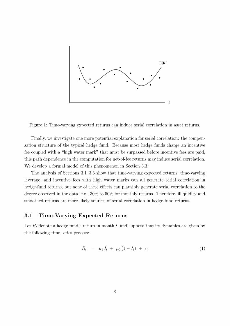
between his current investment policy and other alternatives. Specifically, LeRoy (1973),

Rubinstein (1976), and Lucas (1978) have demonstrated conclusively that serial correlation

in asset returns need not be the result of market inefficiencies, but may be the result of

time-varying expected returns, which is perfectly consistent with the Efficient Markets Hy-

pothesis.4 If an investment strategy’s required expected return varies through time—because

of changes in its risk exposures, for example—then serial correlation may be induced in real-

ized returns without implying any violation of market efficiency (see Figure 1). We examine

this possibility more formally in Section 3.1.

Another possible source of serial correlation in hedge-fund returns is time-varying lever-

age. If managers change the degree to which they leverage their investment strategies, and

if these changes occur in response to lagged market conditions, this is tantamount to time-

varying expected returns. We consider this case in Section 3.2.

4Grossman (1976) and Grossman and Stiglitz (1980) go even further. They argue that perfectly informa-tionally efficient markets are an impossibility, for if markets are perfectly efficient, the return to gatheringinformation is nil, in which case there would be little reason to trade and markets would eventually col-lapse. Alternatively, the degree of market inefficiency determines the effort investors are willing to expendto gather and trade on information, hence a non-degenerate market equilibrium will arise only when thereare sufficient profit opportunities, i.e., inefficiencies, to compensate investors for the costs of trading andinformation-gathering. The profits earned by these attentive investors may be viewed as economic rents thataccrue to those willing to engage in such activities. Who are the providers of these rents? Black (1986) givesa provocative answer: noise traders, individuals who trade on what they think is information but is in factmerely noise.

7

E[Rt]

t

Figure 1: Time-varying expected returns can induce serial correlation in asset returns.

Finally, we investigate one more potential explanation for serial correlation: the compen-

sation structure of the typical hedge fund. Because most hedge funds charge an incentive

fee coupled with a “high water mark” that must be surpassed before incentive fees are paid,

this path dependence in the computation for net-of-fee returns may induce serial correlation.

We develop a formal model of this phenomenon in Section 3.3.

The analysis of Sections 3.1–3.3 show that time-varying expected returns, time-varying

leverage, and incentive fees with high water marks can all generate serial correlation in

hedge-fund returns, but none of these effects can plausibly generate serial correlation to the

degree observed in the data, e.g., 30% to 50% for monthly returns. Therefore, illiquidity and

smoothed returns are more likely sources of serial correlation in hedge-fund returns.

3.1 Time-Varying Expected Returns

Let Rt denote a hedge fund’s return in month t, and suppose that its dynamics are given by

the following time-series process:

Rt = µ1 It + µ0 (1 − It) + εt (1)

8

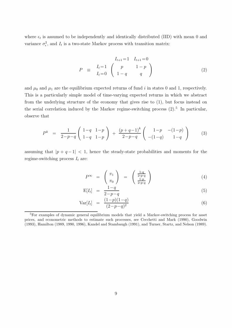
where εt is assumed to be independently and identically distributed (IID) with mean 0 and

variance σ2ε , and It is a two-state Markov process with transition matrix:

P ≡( It+1 =1 It+1 =0

It =1 p 1 − p

It =0 1 − q q

)(2)

and µ0 and µ1 are the equilibrium expected returns of fund i in states 0 and 1, respectively.

This is a particularly simple model of time-varying expected returns in which we abstract

from the underlying structure of the economy that gives rise to (1), but focus instead on

the serial correlation induced by the Markov regime-switching process (2).5 In particular,

observe that

P k =1

2−p−q

(1−q 1−p

1−q 1−p

)+

(p + q−1)k

2−p−q

(1−p −(1−p)

−(1−q) 1−q

)(3)

assuming that |p + q−1| < 1, hence the steady-state probabilities and moments for the

regime-switching process It are:

P∞ =

(π1

π0

)=

(1−q

2−p−q1−p

2−p−q

)(4)

E[It] =1−q

2−p−q(5)

Var[It] =(1−p)(1−q)

(2−p−q)2(6)

5For examples of dynamic general equilibrium models that yield a Markov-switching process for assetprices, and econometric methods to estimate such processes, see Cecchetti and Mark (1990), Goodwin(1993), Hamilton (1989, 1990, 1996), Kandel and Stambaugh (1991), and Turner, Startz, and Nelson (1989).

9

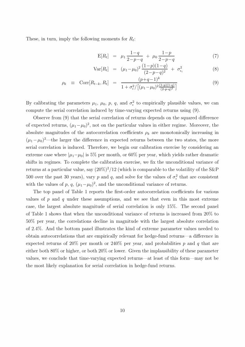
These, in turn, imply the following moments for Rt:

E[Rt] = µ11−q

2−p−q+ µ0

1−p

2−p−q(7)

Var[Rt] = (µ1−µ0)2 (1−p)(1−q)

(2−p−q)2+ σ2

εi(8)

ρk ≡ Corr[Rt−k, Rt] =(p+q−1)k

1 + σ2ε /[(µ1−µ0)2 (1−p)(1−q)

(2−p−q)2

] (9)

By calibrating the parameters µ1, µ0, p, q, and σ2ε to empirically plausible values, we can

compute the serial correlation induced by time-varying expected returns using (9).

Observe from (9) that the serial correlation of returns depends on the squared difference

of expected returns, (µ1−µ0)2, not on the particular values in either regime. Moreover, the

absolute magnitudes of the autocorrelation coefficients ρk are monotonically increasing in

(µ1−µ0)2—the larger the difference in expected returns between the two states, the more

serial correlation is induced. Therefore, we begin our calibration exercise by considering an

extreme case where |µ1−µ0| is 5% per month, or 60% per year, which yields rather dramatic

shifts in regimes. To complete the calibration exercise, we fix the unconditional variance of

returns at a particular value, say (20%)2/12 (which is comparable to the volatility of the S&P

500 over the past 30 years), vary p and q, and solve for the values of σ2ε that are consistent

with the values of p, q, (µ1−µ0)2, and the unconditional variance of returns.

The top panel of Table 1 reports the first-order autocorrelation coefficients for various

values of p and q under these assumptions, and we see that even in this most extreme

case, the largest absolute magnitude of serial correlation is only 15%. The second panel

of Table 1 shows that when the unconditional variance of returns is increased from 20% to

50% per year, the correlations decline in magnitude with the largest absolute correlation

of 2.4%. And the bottom panel illustrates the kind of extreme parameter values needed to

obtain autocorrelations that are empirically relevant for hedge-fund returns—a difference in

expected returns of 20% per month or 240% per year, and probabilities p and q that are

either both 80% or higher, or both 20% or lower. Given the implausibility of these parameter

values, we conclude that time-varying expected returns—at least of this form—may not be

the most likely explanation for serial correlation in hedge-fund returns.

10

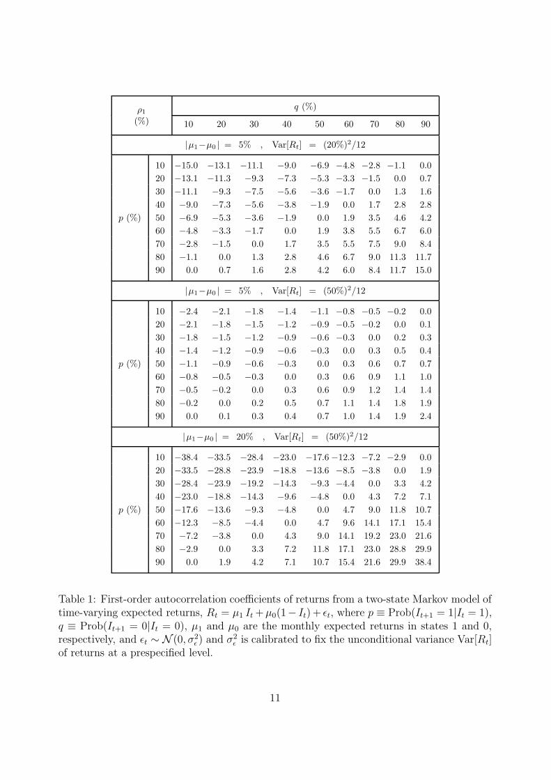
ρ1q (%)

(%) 10 20 30 40 50 60 70 80 90

|µ1−µ0 | = 5% , Var[Rt] = (20%)2/12

10 −15.0 −13.1 −11.1 −9.0 −6.9 −4.8 −2.8 −1.1 0.0

20 −13.1 −11.3 −9.3 −7.3 −5.3 −3.3 −1.5 0.0 0.7

30 −11.1 −9.3 −7.5 −5.6 −3.6 −1.7 0.0 1.3 1.6

40 −9.0 −7.3 −5.6 −3.8 −1.9 0.0 1.7 2.8 2.8

p (%) 50 −6.9 −5.3 −3.6 −1.9 0.0 1.9 3.5 4.6 4.2

60 −4.8 −3.3 −1.7 0.0 1.9 3.8 5.5 6.7 6.0

70 −2.8 −1.5 0.0 1.7 3.5 5.5 7.5 9.0 8.4

80 −1.1 0.0 1.3 2.8 4.6 6.7 9.0 11.3 11.7

90 0.0 0.7 1.6 2.8 4.2 6.0 8.4 11.7 15.0

|µ1−µ0 | = 5% , Var[Rt] = (50%)2/12

10 −2.4 −2.1 −1.8 −1.4 −1.1 −0.8 −0.5 −0.2 0.0

20 −2.1 −1.8 −1.5 −1.2 −0.9 −0.5 −0.2 0.0 0.1

30 −1.8 −1.5 −1.2 −0.9 −0.6 −0.3 0.0 0.2 0.3

40 −1.4 −1.2 −0.9 −0.6 −0.3 0.0 0.3 0.5 0.4

p (%) 50 −1.1 −0.9 −0.6 −0.3 0.0 0.3 0.6 0.7 0.7

60 −0.8 −0.5 −0.3 0.0 0.3 0.6 0.9 1.1 1.0

70 −0.5 −0.2 0.0 0.3 0.6 0.9 1.2 1.4 1.4

80 −0.2 0.0 0.2 0.5 0.7 1.1 1.4 1.8 1.9

90 0.0 0.1 0.3 0.4 0.7 1.0 1.4 1.9 2.4

|µ1−µ0 | = 20% , Var[Rt] = (50%)2/12

10 −38.4 −33.5 −28.4 −23.0 −17.6 −12.3 −7.2 −2.9 0.0

20 −33.5 −28.8 −23.9 −18.8 −13.6 −8.5 −3.8 0.0 1.9

30 −28.4 −23.9 −19.2 −14.3 −9.3 −4.4 0.0 3.3 4.2

40 −23.0 −18.8 −14.3 −9.6 −4.8 0.0 4.3 7.2 7.1

p (%) 50 −17.6 −13.6 −9.3 −4.8 0.0 4.7 9.0 11.8 10.7

60 −12.3 −8.5 −4.4 0.0 4.7 9.6 14.1 17.1 15.4

70 −7.2 −3.8 0.0 4.3 9.0 14.1 19.2 23.0 21.6

80 −2.9 0.0 3.3 7.2 11.8 17.1 23.0 28.8 29.9

90 0.0 1.9 4.2 7.1 10.7 15.4 21.6 29.9 38.4

Table 1: First-order autocorrelation coefficients of returns from a two-state Markov model oftime-varying expected returns, Rt = µ1 It +µ0(1− It) + εt, where p ≡ Prob(It+1 = 1|It = 1),q ≡ Prob(It+1 = 0|It = 0), µ1 and µ0 are the monthly expected returns in states 1 and 0,respectively, and εt ∼ N (0, σ2

ε ) and σ2ε is calibrated to fix the unconditional variance Var[Rt]

of returns at a prespecified level.

11

3.2 Time-Varying Leverage

Another possible source of serial correlation in hedge-fund returns is time-varying leverage.

Since leverage directly affects the expected return of any investment strategy, this can be

considered a special case of the time-varying expected returns model of Section 3.1. Specif-

ically, if Lt denotes a hedge fund’s leverage ratio, then the actual return Rot of the fund at

date t is given by:

Rot = Lt Rt (10)

where Rt is the fund’s unlevered return.6 For example if a fund’s unlevered strategy yields a

2% return in a given month, but 50% of the funds are borrowed from various counterparties

at fixed borrowing rates, the return to the fund’s investors is approximately 4%,7 hence the

leverage ratio is 2.

The specific mechanisms by which a hedge fund determines its leverage can be quite

complex and often depend on a number of factors including market volatility, credit risk,

and various constraints imposed by investors, regulatory bodies, banks, brokers, and other

counterparties. But the basic motivation for typical leverage dynamics is the well-known

trade-off between risk and expected return: by increasing its leverage ratio, a hedge fund

boosts its expected returns proportionally, but also increases its return volatility and, even-

tually, its credit risk or risk of default. Therefore, counterparties providing credit facilities

for hedge funds will impose some ceiling on the degree of leverage they are willing to provide.

More importantly, as market prices move against a hedge fund’s portfolio, thereby reducing

the value of the fund’s collateral and increasing its leverage ratio, or as markets become more

volatile and the fund’s risk exposure increases significantly, creditors (and, in some cases,

securities regulations) will require the fund to either post additional collateral or liquidate

a portion of its portfolio to bring the leverage ratio back down to an acceptable level. As a

result, the leverage ratio of a typical hedge fund varies through time in a specific manner,

usually as a function of market prices and market volatility. Therefore we propose a simple

data-dependent mechanism through which a hedge fund determines its ideal leverage ratio.

Denote by Rt the return of a fund in the absence of any leverage, and to focus squarely

6For simplicity, and with little loss in generality, we have ignored the borrowing costs associated withleverage in our specification (10). Although including such costs will obviously reduce the net return, theserial correlation properties will be largely unaffected because the time variation in borrowing rates is notsignificant relative to Rt and Lt.

7Less the borrowing rate, of course, which we assume is 0 for simplicity.

12

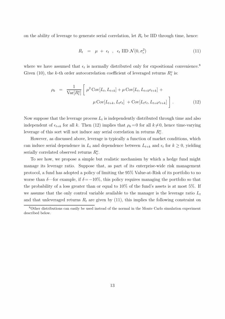
on the ability of leverage to generate serial correlation, let Rt be IID through time, hence:

Rt = µ + εt , εt IID N (0, σ2ε ) (11)

where we have assumed that εt is normally distributed only for expositional convenience.8

Given (10), the k-th order autocorrelation coefficient of leveraged returns Rot is:

ρk =1

Var[Rot ]

[µ2 Cov[Lt, Lt+k] + µ Cov[Lt, Lt+kεt+k] +

µ Cov[Lt+k, Ltεt] + Cov[Ltεt, Lt+kεt+k]

]. (12)

Now suppose that the leverage process Lt is independently distributed through time and also

independent of εt+k for all k. Then (12) implies that ρk =0 for all k 6=0, hence time-varying

leverage of this sort will not induce any serial correlation in returns Rot .

However, as discussed above, leverage is typically a function of market conditions, which

can induce serial dependence in Lt and dependence between Lt+k and εt for k ≥ 0, yielding

serially correlated observed returns Rot .

To see how, we propose a simple but realistic mechanism by which a hedge fund might

manage its leverage ratio. Suppose that, as part of its enterprise-wide risk management

protocol, a fund has adopted a policy of limiting the 95% Value-at-Risk of its portfolio to no

worse than δ—for example, if δ=−10%, this policy requires managing the portfolio so that

the probability of a loss greater than or equal to 10% of the fund’s assets is at most 5%. If

we assume that the only control variable available to the manager is the leverage ratio Lt

and that unleveraged returns Rt are given by (11), this implies the following constraint on

8Other distributions can easily be used instead of the normal in the Monte Carlo simulation experimentdescribed below.

13

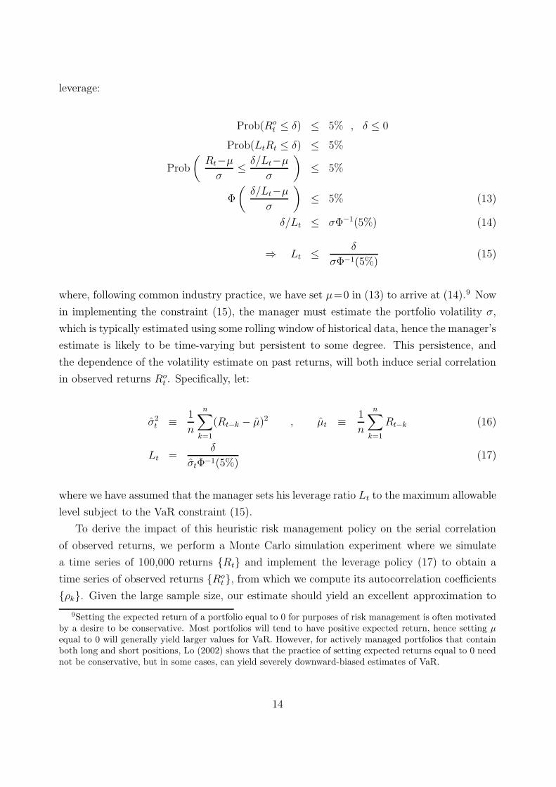
leverage:

Prob(Rot ≤ δ) ≤ 5% , δ ≤ 0

Prob(LtRt ≤ δ) ≤ 5%

Prob

(Rt−µ

σ≤ δ/Lt−µ

σ

)≤ 5%

Φ

(δ/Lt−µ

σ

)≤ 5% (13)

δ/Lt ≤ σΦ−1(5%) (14)

⇒ Lt ≤ δ

σΦ−1(5%)(15)

where, following common industry practice, we have set µ=0 in (13) to arrive at (14).9 Now

in implementing the constraint (15), the manager must estimate the portfolio volatility σ,

which is typically estimated using some rolling window of historical data, hence the manager’s

estimate is likely to be time-varying but persistent to some degree. This persistence, and

the dependence of the volatility estimate on past returns, will both induce serial correlation

in observed returns Rot . Specifically, let:

σ2t ≡ 1

n

n∑

k=1

(Rt−k − µ)2 , µt ≡ 1

n

n∑

k=1

Rt−k (16)

Lt =δ

σtΦ−1(5%)(17)

where we have assumed that the manager sets his leverage ratio Lt to the maximum allowable

level subject to the VaR constraint (15).

To derive the impact of this heuristic risk management policy on the serial correlation

of observed returns, we perform a Monte Carlo simulation experiment where we simulate

a time series of 100,000 returns {Rt} and implement the leverage policy (17) to obtain a

time series of observed returns {Rot }, from which we compute its autocorrelation coefficients

{ρk}. Given the large sample size, our estimate should yield an excellent approximation to

9Setting the expected return of a portfolio equal to 0 for purposes of risk management is often motivatedby a desire to be conservative. Most portfolios will tend to have positive expected return, hence setting µequal to 0 will generally yield larger values for VaR. However, for actively managed portfolios that containboth long and short positions, Lo (2002) shows that the practice of setting expected returns equal to 0 neednot be conservative, but in some cases, can yield severely downward-biased estimates of VaR.

14

the population values of the autocorrelation coefficients. This procedure is performed for

the following combinations of parameter values:

n = 3, 6, 9, 12, 24, 36, 48, 60

12 µ = 5%√

12σ = 10%, 20%, 50%

δ = −25%

and the results are summarized in Table 2. Note that the autocorrelation of observed returns

(12) is homogeneous of degree 0 in δ, hence we need only simulate our return process for

one value of δ without loss of generality as far as ρk is concerned. Of course, the mean and

standard of observed returns and leverage will be affected by our choice of δ, but because

these variables are homogeneous of degree 1, we can obtain results for any arbitrary δ simply

by rescaling our results for δ=−25%.

For a VaR constraint of −25% and an annual standard deviation of unlevered returns

of 10%, the mean leverage ratio ranges from 9.52 when n = 3 to 4.51 when n = 60. For

small n, there is considerably more sampling variation in the estimated standard deviation

of returns, hence the leverage ratio—which is proportional to the reciprocal of σt—takes on

more extreme values as well and has a higher expectation in this case.

As n increases, the volatility estimator becomes more stable over time since each month’s

estimator has more data in common with the previous month’s estimator, leading to more

persistence in Lt as expected. For example, when n=3, the average first-order autocorrela-

tion coefficient of Lt is 43.2%, but increases to 98.2% when n=60. However, even with such

extreme levels of persistence in Lt, the autocorrelation induced in observed returns Rot is still

only −0.2%. In fact, the largest absolute return-autocorrelation reported in Table 2 is only

0.7%, despite the fact that leverage ratios are sometimes nearly perfectly autocorrelated from

month to month. This suggests that time-varying leverage, at least of the form described

by the VaR constraint (15), cannot fully account for the magnitudes of serial correlation in

historical hedge-fund returns.

3.3 Incentive Fees with High-Water Marks

Yet another source of serial correlation in hedge-fund returns is an aspect of the fee structure

that is commonly used in the hedge-fund industry: an incentive fee—typically 20% of excess

returns above a benchmark—which is subject to a “high-water mark”, meaning that incentive

15

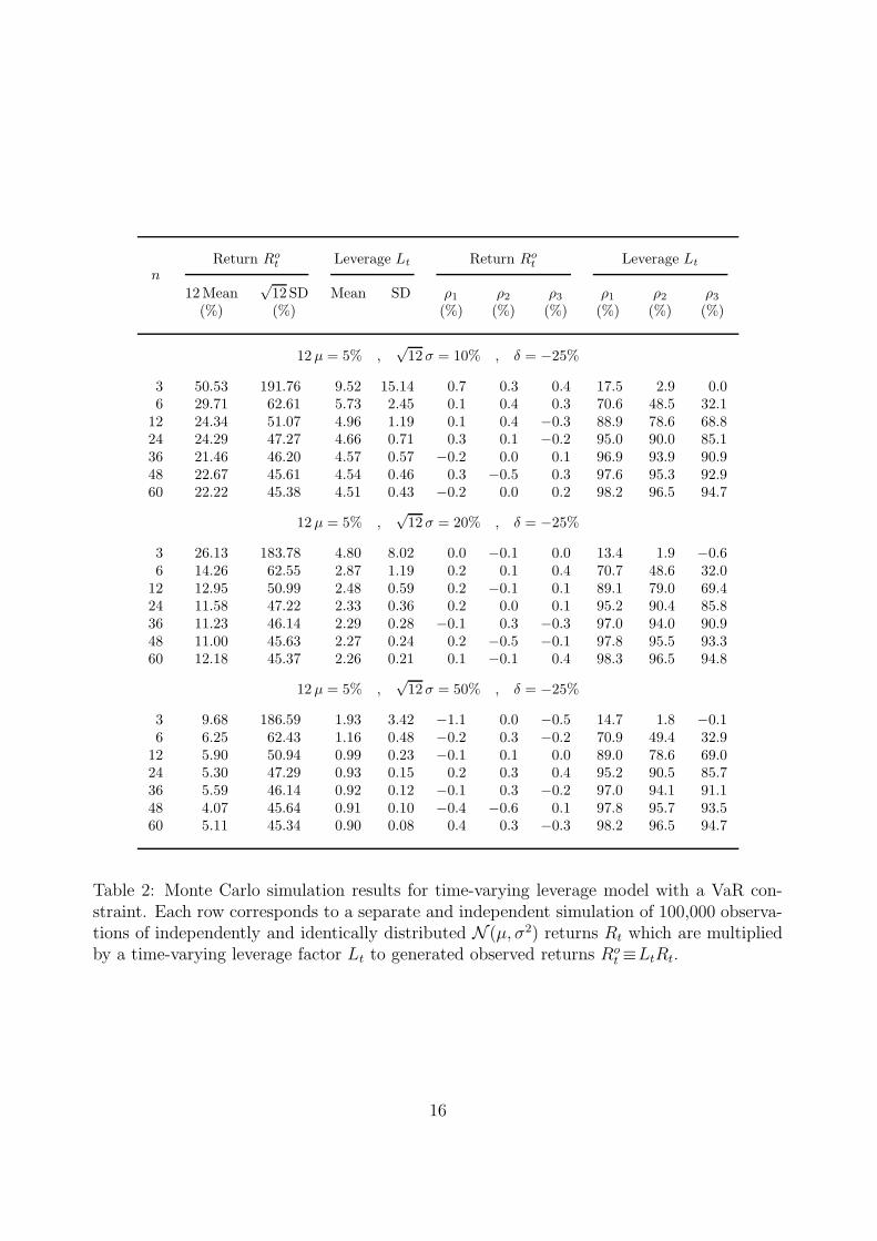
nReturn Ro

t Leverage Lt Return Rot Leverage Lt

12 Mean√

12SD Mean SD ρ1 ρ2 ρ3 ρ1 ρ2 ρ3

(%) (%) (%) (%) (%) (%) (%) (%)

12 µ = 5% ,√

12σ = 10% , δ = −25%

3 50.53 191.76 9.52 15.14 0.7 0.3 0.4 17.5 2.9 0.06 29.71 62.61 5.73 2.45 0.1 0.4 0.3 70.6 48.5 32.1

12 24.34 51.07 4.96 1.19 0.1 0.4 −0.3 88.9 78.6 68.824 24.29 47.27 4.66 0.71 0.3 0.1 −0.2 95.0 90.0 85.136 21.46 46.20 4.57 0.57 −0.2 0.0 0.1 96.9 93.9 90.948 22.67 45.61 4.54 0.46 0.3 −0.5 0.3 97.6 95.3 92.960 22.22 45.38 4.51 0.43 −0.2 0.0 0.2 98.2 96.5 94.7

12 µ = 5% ,√

12σ = 20% , δ = −25%

3 26.13 183.78 4.80 8.02 0.0 −0.1 0.0 13.4 1.9 −0.66 14.26 62.55 2.87 1.19 0.2 0.1 0.4 70.7 48.6 32.0

12 12.95 50.99 2.48 0.59 0.2 −0.1 0.1 89.1 79.0 69.424 11.58 47.22 2.33 0.36 0.2 0.0 0.1 95.2 90.4 85.836 11.23 46.14 2.29 0.28 −0.1 0.3 −0.3 97.0 94.0 90.948 11.00 45.63 2.27 0.24 0.2 −0.5 −0.1 97.8 95.5 93.360 12.18 45.37 2.26 0.21 0.1 −0.1 0.4 98.3 96.5 94.8

12 µ = 5% ,√

12σ = 50% , δ = −25%

3 9.68 186.59 1.93 3.42 −1.1 0.0 −0.5 14.7 1.8 −0.16 6.25 62.43 1.16 0.48 −0.2 0.3 −0.2 70.9 49.4 32.9

12 5.90 50.94 0.99 0.23 −0.1 0.1 0.0 89.0 78.6 69.024 5.30 47.29 0.93 0.15 0.2 0.3 0.4 95.2 90.5 85.736 5.59 46.14 0.92 0.12 −0.1 0.3 −0.2 97.0 94.1 91.148 4.07 45.64 0.91 0.10 −0.4 −0.6 0.1 97.8 95.7 93.560 5.11 45.34 0.90 0.08 0.4 0.3 −0.3 98.2 96.5 94.7

Table 2: Monte Carlo simulation results for time-varying leverage model with a VaR con-straint. Each row corresponds to a separate and independent simulation of 100,000 observa-tions of independently and identically distributed N (µ, σ2) returns Rt which are multipliedby a time-varying leverage factor Lt to generated observed returns Ro

t ≡LtRt.

16

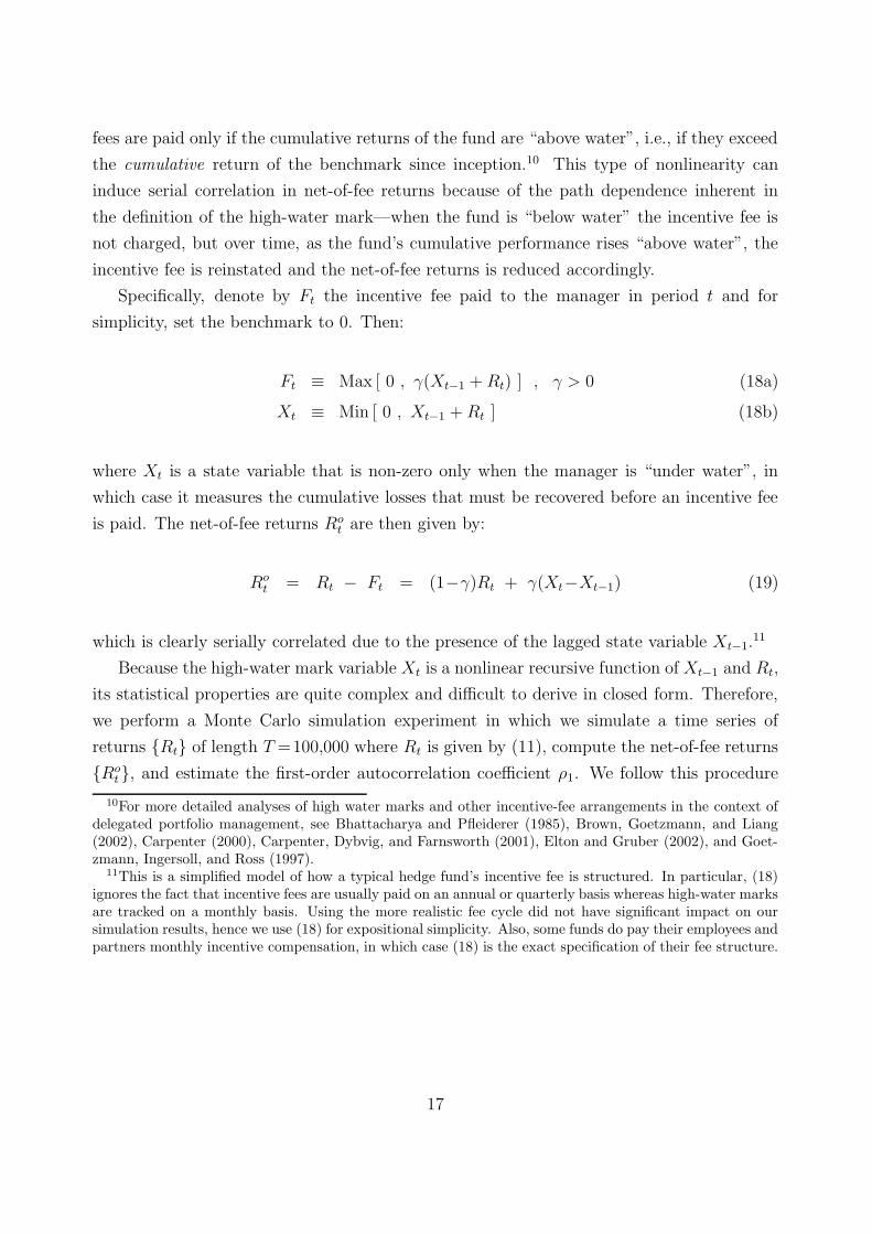
fees are paid only if the cumulative returns of the fund are “above water”, i.e., if they exceed

the cumulative return of the benchmark since inception.10 This type of nonlinearity can

induce serial correlation in net-of-fee returns because of the path dependence inherent in

the definition of the high-water mark—when the fund is “below water” the incentive fee is

not charged, but over time, as the fund’s cumulative performance rises “above water”, the

incentive fee is reinstated and the net-of-fee returns is reduced accordingly.

Specifically, denote by Ft the incentive fee paid to the manager in period t and for

simplicity, set the benchmark to 0. Then:

Ft ≡ Max [ 0 , γ(Xt−1 + Rt) ] , γ > 0 (18a)

Xt ≡ Min [ 0 , Xt−1 + Rt ] (18b)

where Xt is a state variable that is non-zero only when the manager is “under water”, in

which case it measures the cumulative losses that must be recovered before an incentive fee

is paid. The net-of-fee returns Rot are then given by:

Rot = Rt − Ft = (1−γ)Rt + γ(Xt−Xt−1) (19)

which is clearly serially correlated due to the presence of the lagged state variable Xt−1.11

Because the high-water mark variable Xt is a nonlinear recursive function of Xt−1 and Rt,

its statistical properties are quite complex and difficult to derive in closed form. Therefore,

we perform a Monte Carlo simulation experiment in which we simulate a time series of

returns {Rt} of length T =100,000 where Rt is given by (11), compute the net-of-fee returns

{Rot}, and estimate the first-order autocorrelation coefficient ρ1. We follow this procedure

10For more detailed analyses of high water marks and other incentive-fee arrangements in the context ofdelegated portfolio management, see Bhattacharya and Pfleiderer (1985), Brown, Goetzmann, and Liang(2002), Carpenter (2000), Carpenter, Dybvig, and Farnsworth (2001), Elton and Gruber (2002), and Goet-zmann, Ingersoll, and Ross (1997).

11This is a simplified model of how a typical hedge fund’s incentive fee is structured. In particular, (18)ignores the fact that incentive fees are usually paid on an annual or quarterly basis whereas high-water marksare tracked on a monthly basis. Using the more realistic fee cycle did not have significant impact on oursimulation results, hence we use (18) for expositional simplicity. Also, some funds do pay their employees andpartners monthly incentive compensation, in which case (18) is the exact specification of their fee structure.

17

for each of the combinations of the following parameter values:

12 µ = 5%, 10%, 15%, . . . , 50%√

12σ = 10%, 20%, . . . , 50%

γ = 20% .

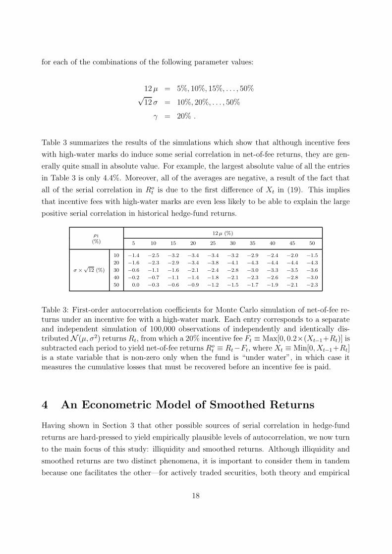
Table 3 summarizes the results of the simulations which show that although incentive fees

with high-water marks do induce some serial correlation in net-of-fee returns, they are gen-

erally quite small in absolute value. For example, the largest absolute value of all the entries

in Table 3 is only 4.4%. Moreover, all of the averages are negative, a result of the fact that

all of the serial correlation in Rot is due to the first difference of Xt in (19). This implies

that incentive fees with high-water marks are even less likely to be able to explain the large

positive serial correlation in historical hedge-fund returns.

ρ112 µ (%)

(%) 5 10 15 20 25 30 35 40 45 50

10 −1.4 −2.5 −3.2 −3.4 −3.4 −3.2 −2.9 −2.4 −2.0 −1.5

20 −1.6 −2.3 −2.9 −3.4 −3.8 −4.1 −4.3 −4.4 −4.4 −4.3

σ ×√

12 (%) 30 −0.6 −1.1 −1.6 −2.1 −2.4 −2.8 −3.0 −3.3 −3.5 −3.6

40 −0.2 −0.7 −1.1 −1.4 −1.8 −2.1 −2.3 −2.6 −2.8 −3.0

50 0.0 −0.3 −0.6 −0.9 −1.2 −1.5 −1.7 −1.9 −2.1 −2.3

Table 3: First-order autocorrelation coefficients for Monte Carlo simulation of net-of-fee re-turns under an incentive fee with a high-water mark. Each entry corresponds to a separateand independent simulation of 100,000 observations of independently and identically dis-tributed N (µ, σ2) returns Rt, from which a 20% incentive fee Ft ≡ Max[0, 0.2×(Xt−1+Rt)] issubtracted each period to yield net-of-fee returns Ro

t ≡ Rt−Ft, where Xt ≡ Min[0, Xt−1+Rt]is a state variable that is non-zero only when the fund is “under water”, in which case itmeasures the cumulative losses that must be recovered before an incentive fee is paid.

4 An Econometric Model of Smoothed Returns

Having shown in Section 3 that other possible sources of serial correlation in hedge-fund

returns are hard-pressed to yield empirically plausible levels of autocorrelation, we now turn

to the main focus of this study: illiquidity and smoothed returns. Although illiquidity and

smoothed returns are two distinct phenomena, it is important to consider them in tandem

because one facilitates the other—for actively traded securities, both theory and empirical

18

evidence suggest that in the absence of transactions costs and other market frictions, returns

are unlikely to be very smooth.

As we argued in Section 1, nonsynchronous trading is a plausible source of serial corre-

lation in hedge-fund returns. In contrast to the studies by Lo and MacKinlay (1988, 1990)

and Kadlec and Patterson (1999) in which they conclude that it is difficult to generate serial

correlations in weekly US equity portfolio returns much greater than 10% to 15% through

nonsynchronous trading effects alone, we argue that in the context of hedge funds, signifi-

cantly higher levels of serial correlation can be explained by the combination of illiquidity

and smoothed returns, of which nonsynchronous trading is a special case. To see why, note

that the empirical analysis in the nonsynchronous-trading literature is devoted exclusively to

exchange-traded equity returns, not hedge-fund returns, hence their conclusions may not be

relevant in our context. For example, Lo and MacKinlay (1990) argue that securities would

have to go without trading for several days on average to induce serial correlations of 30%,

and they dismiss such nontrading intervals as unrealistic for most exchange-traded US eq-

uity issues. However, such nontrading intervals are considerably more realistic for the types

of securities held by many hedge funds, e.g., emerging-market debt, real estate, restricted

securities, control positions in publicly traded companies, asset-backed securities, and other

exotic OTC derivatives. Therefore, nonsynchronous trading of this magnitude is likely to be

an explanation for the serial correlation observed in hedge-fund returns.

But even when prices are synchronously measured—as they are for many funds that mark

their portfolios to market at the end of the month to strike a net-asset-value at which investors

can buy into or cash out of the fund—there are several other channels by which illiquidity

exposure can induce serial correlation in the reported returns of hedge funds. Apart from

the nonsynchronous-trading effect, naive methods for determining the fair market value or

“marks” for illiquid securities can yield serially correlated returns. For example, one approach

to valuing illiquid securities is to extrapolate linearly from the most recent transaction price

(which, in the case of emerging-market debt, might be several months ago), which yields

a price path that is a straight line, or at best a series of straight lines. Returns computed

from such marks will be smoother, exhibiting lower volatility and higher serial correlation

than true economic returns, i.e., returns computed from mark-to-market prices where the

market is sufficiently active to allow all available information to be impounded in the price of

the security. Of course, for securities that are more easily traded and with deeper markets,

mark-to-market prices are more readily available, extrapolated marks are not necessary, and

serial correlation is therefore less of an issue. But for securities that are thinly traded, or not

traded at all for extended periods of time, marking them to market is often an expensive and

time-consuming procedure that cannot easily be performed frequently. Therefore, we argue

19

in this paper that serial correlation may serve as a proxy for a fund’s liquidity exposure.

Even if a hedge-fund manager does not make use of any form of linear extrapolation to

mark the securities in his portfolio, he may still be subject to smoothed returns if he obtains

marks from broker-dealers that engage in such extrapolation. For example, consider the

case of a conscientious hedge-fund manager attempting to obtain the most accurate mark

for his portfolio at month end by getting bid/offer quotes from three independent broker-

dealers for every security in his portfolio, and then marking each security at the average of

the three quote midpoints. By averaging the quote midpoints, the manager is inadvertently

downward-biasing price volatility, and if any of the broker-dealers employ linear extrapolation

in formulating their quotes (and many do, through sheer necessity because they have little

else to go on for the most illiquid securities), or if they fail to update their quotes because

of light volume, serial correlation will also be induced in reported returns.

Finally, a more prosaic channel by which serial correlation may arise in the reported re-

turns of hedge funds is through “performance smoothing”, the unsavory practice of reporting

only part of the gains in months when a fund has positive returns so as to partially offset

potential future losses and thereby reduce volatility and improve risk-adjusted performance

measures such as the Sharpe ratio. For funds containing liquid securities that can be easily

marked to market, performance smoothing is more difficult and, as a result, less of a con-

cern. Indeed, it is only for portfolios of illiquid securities that managers and brokers have

any discretion in marking their positions. Such practices are generally prohibited by various

securities laws and accounting principles, and great care must be exercised in interpreting

smoothed returns as deliberate attempts to manipulate performance statistics. After all, as

we have discussed above, there are many other sources of serial correlation in the presence

of illiquidity, none of which is motivated by deceit. Nevertheless, managers do have certain

degrees of freedom in valuing illiquid securities—for example, discretionary accruals for un-

registered private placements and venture capital investments—and Chandar and Bricker

(2002) conclude that managers of certain closed-end mutual funds do use accounting dis-

cretion to manage fund returns around a passive benchmark. Therefore, the possibility of

deliberate performance smoothing in the less regulated hedge-fund industry must be kept in

mind in interpreting our empirical analysis of smoothed returns.

To quantify the impact of all of these possible sources of serial correlation, denote by Rt

the true economic return of a hedge fund in period t, and let Rt satisfy the following linear

20

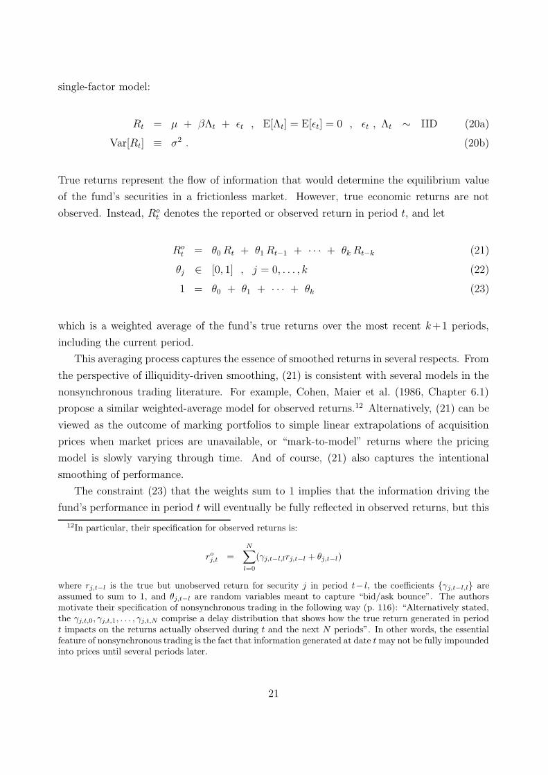
single-factor model:

Rt = µ + βΛt + εt , E[Λt] = E[εt] = 0 , εt , Λt ∼ IID (20a)

Var[Rt] ≡ σ2 . (20b)

True returns represent the flow of information that would determine the equilibrium value

of the fund’s securities in a frictionless market. However, true economic returns are not

observed. Instead, Rot denotes the reported or observed return in period t, and let

Rot = θ0 Rt + θ1 Rt−1 + · · · + θk Rt−k (21)

θj ∈ [0, 1] , j = 0, . . . , k (22)

1 = θ0 + θ1 + · · · + θk (23)

which is a weighted average of the fund’s true returns over the most recent k+1 periods,

including the current period.

This averaging process captures the essence of smoothed returns in several respects. From

the perspective of illiquidity-driven smoothing, (21) is consistent with several models in the

nonsynchronous trading literature. For example, Cohen, Maier et al. (1986, Chapter 6.1)

propose a similar weighted-average model for observed returns.12 Alternatively, (21) can be

viewed as the outcome of marking portfolios to simple linear extrapolations of acquisition

prices when market prices are unavailable, or “mark-to-model” returns where the pricing

model is slowly varying through time. And of course, (21) also captures the intentional

smoothing of performance.

The constraint (23) that the weights sum to 1 implies that the information driving the

fund’s performance in period t will eventually be fully reflected in observed returns, but this

12In particular, their specification for observed returns is:

roj,t =

N∑

l=0

(γj,t−l,lrj,t−l + θj,t−l)

where rj,t−l is the true but unobserved return for security j in period t− l, the coefficients {γj,t−l,l} areassumed to sum to 1, and θj,t−l are random variables meant to capture “bid/ask bounce”. The authorsmotivate their specification of nonsynchronous trading in the following way (p. 116): “Alternatively stated,the γj,t,0, γj,t,1, . . . , γj,t,N comprise a delay distribution that shows how the true return generated in periodt impacts on the returns actually observed during t and the next N periods”. In other words, the essentialfeature of nonsynchronous trading is the fact that information generated at date t may not be fully impoundedinto prices until several periods later.

21

process could take up to k+1 periods from the time the information is generated.13 This

is a sensible restriction in the current context of hedge funds for several reasons. Even the

most illiquid securities will trade eventually, and when that occurs, all of the cumulative

information affecting that security will be fully impounded into its transaction price. There-

fore the parameter k should be selected to match the kind of illiquidity of the fund—a fund

comprised mostly of exchange-traded US equities would require a much lower value of k than

a private equity fund. Alternatively, in the case of intentional smoothing of performance,

the necessity of periodic external audits of fund performance imposes a finite limit on the

extent to which deliberate smoothing can persist.14

4.1 Implications For Performance Statistics

Given the smoothing mechanism outlined above, we have the following implications for the

statistical properties of observed returns:

Proposition 1 Under (21)–(23), the statistical properties of observed returns are charac-

13In Lo and MacKinlay’s (1990) model of nonsynchronous trading, they propose a stochastic non-tradinghorizon so that observed returns are an infinite-order moving average of past true returns, where the coeffi-cients are stochastic. In that framework, the waiting time for information to become fully impounded intofuture returns may be arbitrarily long (but with increasingly remote probability).

14In fact, if a fund allows investors to invest and withdraw capital only at pre-specified intervals, imposinglock-ups in between, and external audits are conducted at these same pre-specified intervals, then it maybe argued that performance smoothing is irrelevant. For example, no investor should be disadvantagedby investing in a fund that offers annual liquidity and engages in annual external audits with which thefund’s net-asset-value is determined by a disinterested third party for purposes of redemptions and newinvestments. However, there are at least two additional concerns that remain—historical track records arestill affected by smoothed returns, and estimates of a fund’s liquidity exposure are also affected—both ofwhich are important factors in the typical hedge-fund investor’s overall investment process. Moreover, giventhe apparently unscrupulous role that the auditors at Arthur Andersen played in the Enron affair, there isthe further concern of whether third-party auditors are truly objective and free of all conflicts of interest.

22

terized by:

E[Rot ] = µ (24)

Var[Rot ] = c2

σ σ2 ≤ σ2 (25)

SRo ≡ E[Rot ]√

Var[Rot ]

= cs SR ≥ SR ≡ E[Rt]√Var[Rt]

(26)

βom ≡ Cov[Ro

t , Λt−m]

Var[Λt−m]=

cβ,m β if 0 ≤ m ≤ k

0 if m > k(27)

Cov[Rot , R

ot−m] =

(∑k−mj=0 θjθj+m

)σ2 if 0 ≤ m ≤ k

0 if m > k(28)

Corr[Rot , R

ot−m] =

Cov[Rot , R

ot−m]

Var[Rot ]

=

∑k−mj=0 θjθj+m∑k

j=0 θ2j

if 0 ≤ m ≤ k

0 if m > k(29)

where:

cµ ≡ θ0 + θ1 + · · · + θk (30)

c2σ ≡ θ2

0 + θ21 + · · · + θ2

k (31)

cs ≡ 1/√

θ20 + · · ·+ θ2

k (32)

cβ,m ≡ θm (33)

Proposition 1 shows that smoothed returns of the form (21)–(23) do not affect the expected

value of Rot but reduce its variance, hence boosting the Sharpe ratio of observed returns

by a factor of cs. From (27), we see that smoothing also affects βo0 , the contemporaneous

market beta of observed returns, biasing it towards 0 or “market neutrality”, and induces

correlation between current observed returns and lagged market returns up to lag k. This

provides a formal interpretation of the empirical analysis of Asness, Krail, and Liew (2001)

in which many hedge funds were found to have significant lagged market exposure despite

relatively low contemporaneous market betas.

23

Smoothed returns also exhibit positive serial correlation up to order k according to (29),

and the magnitude of the effect is determined by the pattern of weights {θj}. If, for example,

the weights are disproportionately centered on a small number of lags, relatively little serial

correlation will be induced. However, if the weights are evenly distributed among many lags,

this will result in higher serial correlation. A useful summary statistic for measuring the

concentration of weights is

ξ ≡k∑

j=0

θ2j ∈ [0, 1] (34)

which is simply the denominator of (29). This measure is well known in the industrial

organization literature as the Herfindahl index, a measure of the concentration of firms in a

given industry where θj represents the market share of firm j. Because θj ∈ [0, 1], ξ is also

confined to the unit interval, and is minimized when all the θj’s are identical, which implies

a value of 1/(k+1) for ξ, and is maximized when one coefficient is 1 and the rest are 0,

in which case ξ = 1. In the context of smoothed returns, a lower value of ξ implies more

smoothing, and the upper bound of 1 implies no smoothing, hence we shall refer to ξ as a

“smoothing index”.

In the special case of equal weights, θj = 1/(k+1) for j =0, . . . , k, the serial correlation

of observed returns takes on a particularly simple form:

Corr[Rot , R

ot−m] = 1 − m

k + 1, 1 ≤ m ≤ k (35)

which declines linearly in the lag m. This can yield substantial correlations even when k

is small—for example, if k = 2 so that smoothing takes place only over a current quarter

(i.e. this month and the previous two months), the first-order autocorrelation of monthly

observed returns is 66.7%.

To develop a sense for just how much observed returns can differ from true returns

under the smoothed-return mechanism (21)–(23), denote by ∆(T ) the difference between

the cumulative observed and true returns over T holding periods, where we assume that

24

T >k:

∆(T ) ≡ (Ro1 + Ro

2 + · · · + RoT ) − (R1 + R2 + · · · + RT ) (36)

=

k−1∑

j=0

(R−j − RT−j)(1 −j∑

i=0

θi) (37)

Then we have:

Proposition 2 Under (21)–(23) and for T > k,

E[∆(T )] = 0 (38)

Var[∆(T )] = 2σ2k−1∑

j=0

(1 −

j∑

l=0

θl

)2

= 2σ2 ζ (39)

ζ ≡k−1∑

j=0

(1 −

j∑

l=0

θl

)2

≤ k (40)

Proposition 2 shows that the cumulative difference between observed and true returns has 0

expected value, and its variance is bounded above by 2kσ2.

4.2 Examples of Smoothing Profiles

To develop further intuition for the impact of smoothed returns on observed returns, we

consider the following three specific sets of weights {θj} or “smoothing profiles”:15

θj =1

k + 1(Straightline) (41)

θj =k + 1 − j

(k + 1)(k + 2)/2(Sum-of-Years) (42)

θj =δj(1 − δ)

1 − δk+1, δ ∈ (0, 1) (Geometric) . (43)

The straightline profile weights each return equally. In contrast, the sum-of-years and ge-

ometric profiles weight the current return the most heavily, and then has monotonically

15Students of accounting will recognize these profiles as commonly used methods for computing deprecia-tion. The motivation for these depreciation schedules is not entirely without relevance in the smoothed-returncontext.

25

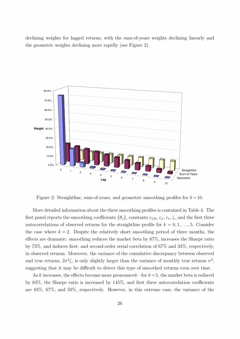
declining weights for lagged returns, with the sum-of-years weights declining linearly and

the geometric weights declining more rapidly (see Figure 2).

0 1 2 3 4 5 6 7 8 9 10

GeometricSum-of-Years

Straightline

0.0%

10.0%

20.0%

30.0%

40.0%

50.0%

60.0%

70.0%

80.0%

Weight

Lag

Figure 2: Straightline, sum-of-years, and geometric smoothing profiles for k=10.

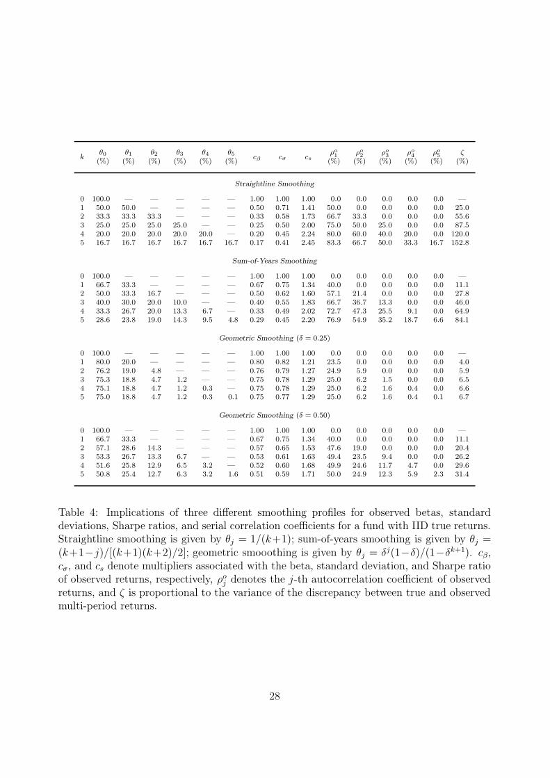
More detailed information about the three smoothing profiles is contained in Table 4. The

first panel reports the smoothing coefficients {θj}, constants cβ,0, cσ, cs, ζ, and the first three

autocorrelations of observed returns for the straightline profile for k = 0, 1, . . . , 5. Consider

the case where k = 2. Despite the relatively short smoothing period of three months, the

effects are dramatic: smoothing reduces the market beta by 67%, increases the Sharpe ratio

by 73%, and induces first- and second-order serial correlation of 67% and 33%, respectively,

in observed returns. Moreover, the variance of the cumulative discrepancy between observed

and true returns, 2σ2ζ, is only slightly larger than the variance of monthly true returns σ2,

suggesting that it may be difficult to detect this type of smoothed returns even over time.

As k increases, the effects become more pronounced—for k=5, the market beta is reduced

by 83%, the Sharpe ratio is increased by 145%, and first three autocorrelation coefficients

are 83%, 67%, and 50%, respectively. However, in this extreme case, the variance of the

26

discrepancy between true and observed returns is approximately three times the monthly

variance of true returns, in which case it may be easier to identify smoothing from realized

returns.

The sum-of-years profile is similar to, although somewhat less extreme than, the straight-

line profile for the same values of k because more weight is being placed on the current return.

For example, even in the extreme case of k=5, the sum-of-years profile reduces the market

beta by 71%, increases the Sharpe ratio by 120%, induces autocorrelations of 77%, 55%, and

35%, respectively, in the first three lags, and has a discrepancy variance that is approximately

1.6 times the monthly variance of true returns.

The last two panels of Table 4 contain results for the geometric smoothing profile for

two values of δ, 0.25 and 0.50. For δ=0.25, the geometric profile places more weight on the

current return than the other two smoothing profiles for all values of k, hence the effects

tend to be less dramatic. Even in the extreme case of k=5, 75% of current true returns are

incorporated into observed returns, the market beta is reduced by only 25%, the Sharpe ratio

is increased by only 29%, the first three autocorrelations are 25%, 6%, and 1% respectively,

and the discrepancy variance is approximately 13% of the monthly variance of true returns.

As δ increases, less weight is placed on the current observation and the effects on performance

statistics become more significant. When δ = 0.50 and k = 5, geometric smoothing reduces

the market beta by 49%, increases the Sharpe ratio by 71%, induces autocorrelations of 50%,

25%, and 12%, respectively, for the first three lags, and yields a discrepancy variance that

is approximately 63% of the monthly variance of true returns.

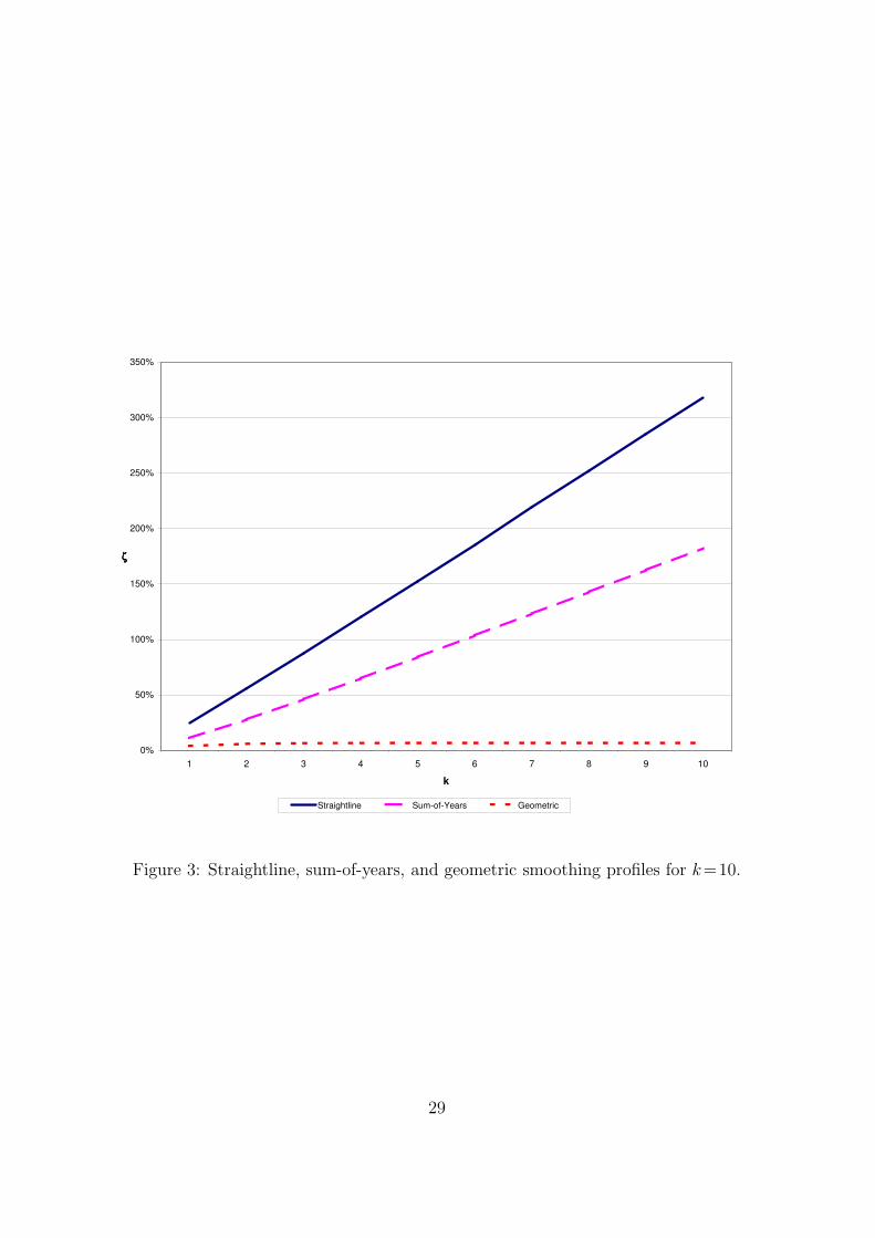
The three smoothing profiles have very different values for ζ in (40):

ζ =k(2k + 1)

6(k + 1)(44)

ζ =k(3k2 + 6k + 1)

15(k + 1)(k + 2)(45)

ζ =δ2(−1 + δk(2 + 2δ + δk(−1 − 2δ + k(δ2 − 1))))

(δ2 − 1)(δk+1 − 1)2(46)

with the straightline and sum-of-years profiles implying variances for ∆(T ) that grow approx-

imately linearly in k, and the geometric profile implying a variance for ∆(T ) that asymptotes

to a finite limit (see Figure 3).

The results in Table 4 and Figure 3 show that a rich set of biases can be generated by

even simple smoothing profiles, and even the most casual empirical observation suggests that

smoothed returns may be an important source of serial correlation in hedge-fund returns.

27

kθ0 θ1 θ2 θ3 θ4 θ5 cβ cσ cs

ρo1 ρo

2 ρo3 ρo

4 ρo5 ζ

(%) (%) (%) (%) (%) (%) (%) (%) (%) (%) (%) (%)

Straightline Smoothing

0 100.0 — — — — — 1.00 1.00 1.00 0.0 0.0 0.0 0.0 0.0 —1 50.0 50.0 — — — — 0.50 0.71 1.41 50.0 0.0 0.0 0.0 0.0 25.02 33.3 33.3 33.3 — — — 0.33 0.58 1.73 66.7 33.3 0.0 0.0 0.0 55.63 25.0 25.0 25.0 25.0 — — 0.25 0.50 2.00 75.0 50.0 25.0 0.0 0.0 87.54 20.0 20.0 20.0 20.0 20.0 — 0.20 0.45 2.24 80.0 60.0 40.0 20.0 0.0 120.05 16.7 16.7 16.7 16.7 16.7 16.7 0.17 0.41 2.45 83.3 66.7 50.0 33.3 16.7 152.8

Sum-of-Years Smoothing

0 100.0 — — — — — 1.00 1.00 1.00 0.0 0.0 0.0 0.0 0.0 —1 66.7 33.3 — — — — 0.67 0.75 1.34 40.0 0.0 0.0 0.0 0.0 11.12 50.0 33.3 16.7 — — — 0.50 0.62 1.60 57.1 21.4 0.0 0.0 0.0 27.83 40.0 30.0 20.0 10.0 — — 0.40 0.55 1.83 66.7 36.7 13.3 0.0 0.0 46.04 33.3 26.7 20.0 13.3 6.7 — 0.33 0.49 2.02 72.7 47.3 25.5 9.1 0.0 64.95 28.6 23.8 19.0 14.3 9.5 4.8 0.29 0.45 2.20 76.9 54.9 35.2 18.7 6.6 84.1

Geometric Smoothing (δ = 0.25)

0 100.0 — — — — — 1.00 1.00 1.00 0.0 0.0 0.0 0.0 0.0 —1 80.0 20.0 — — — — 0.80 0.82 1.21 23.5 0.0 0.0 0.0 0.0 4.02 76.2 19.0 4.8 — — — 0.76 0.79 1.27 24.9 5.9 0.0 0.0 0.0 5.93 75.3 18.8 4.7 1.2 — — 0.75 0.78 1.29 25.0 6.2 1.5 0.0 0.0 6.54 75.1 18.8 4.7 1.2 0.3 — 0.75 0.78 1.29 25.0 6.2 1.6 0.4 0.0 6.65 75.0 18.8 4.7 1.2 0.3 0.1 0.75 0.77 1.29 25.0 6.2 1.6 0.4 0.1 6.7

Geometric Smoothing (δ = 0.50)

0 100.0 — — — — — 1.00 1.00 1.00 0.0 0.0 0.0 0.0 0.0 —1 66.7 33.3 — — — — 0.67 0.75 1.34 40.0 0.0 0.0 0.0 0.0 11.12 57.1 28.6 14.3 — — — 0.57 0.65 1.53 47.6 19.0 0.0 0.0 0.0 20.43 53.3 26.7 13.3 6.7 — — 0.53 0.61 1.63 49.4 23.5 9.4 0.0 0.0 26.24 51.6 25.8 12.9 6.5 3.2 — 0.52 0.60 1.68 49.9 24.6 11.7 4.7 0.0 29.65 50.8 25.4 12.7 6.3 3.2 1.6 0.51 0.59 1.71 50.0 24.9 12.3 5.9 2.3 31.4

Table 4: Implications of three different smoothing profiles for observed betas, standarddeviations, Sharpe ratios, and serial correlation coefficients for a fund with IID true returns.Straightline smoothing is given by θj = 1/(k+1); sum-of-years smoothing is given by θj =(k+1−j)/[(k+1)(k+2)/2]; geometric smooothing is given by θj = δj(1−δ)/(1−δk+1). cβ,cσ, and cs denote multipliers associated with the beta, standard deviation, and Sharpe ratioof observed returns, respectively, ρo

j denotes the j-th autocorrelation coefficient of observedreturns, and ζ is proportional to the variance of the discrepancy between true and observedmulti-period returns.

28

0%

50%

100%

150%

200%

250%

300%

350%

1 2 3 4 5 6 7 8 9 10

k

ζζζζ

Straightline Sum-of-Years Geometric

Figure 3: Straightline, sum-of-years, and geometric smoothing profiles for k=10.

29

To address this issue directly, we propose methods for estimating the smoothing profile in

Section 5 and apply these methods to the data in Section 6.

5 Estimation of Smoothing Profiles and Sharpe Ratios

Although the smoothing profiles described in Section 4.2 can all be easily estimated from the

sample moments of fund returns, e.g., means, variances, and autocorrelations, we wish to

be able to estimate more general forms of smoothing. Therefore, in this section we propose

two estimation procedures—maximum likelihood and linear regression—that place fewer

restrictions on a fund’s smoothing profile than the three examples in Section 4.2. In Section

5.1 we review the steps for maximum likelihood estimation of an MA(k) process, slightly

modified to accommodate our context and constraints, and in Section 5.2 we consider a

simpler alternative based on linear regression under the assumption that true returns are

generated by the linear single-factor model (20). We propose several specification checks to

evaluate the robustness of our smoothing model in Section 5.3, and in Section 5.4 we show

how to adjust Sharpe ratios to take smoothed returns into account.

5.1 Maximum Likelihood Estimation

Given the specification of the smoothing process in (21)–(23), we can estimate the smoothing

profile using maximum likelihood estimation in a fashion similar to the estimation of standard

moving-average time series models (see, for example, Brockwell and Davis, 1991, Chapter

8). We begin by defining the de-meaned observed returns process Xt:

Xt = Rot − µ (47)

and observing that (21)–(23) implies the following properties for Xt:

Xt = θ0ηt + θ1ηt−1 + · · · + θkηt−k (48)

1 = θ0 + θ1 + · · · + θk (49)

ηk ∼ N (0, σ2η) (50)

where, for purposes of estimation, we have added the parametric assumption (50) that ηk

is normally distributed. From (48), it is apparent that Xt is a moving-average process of

order k, or an “MA(k)”. For a given set of observations X ≡ [ X1 · · · XT ]′, the likelihood

30

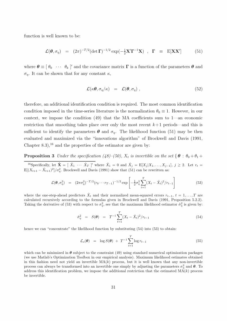
function is well known to be:

L(θ, ση) = (2π)−T/2(detΓ)−1/2 exp(−12X′Γ−1X) , Γ ≡ E[XX′] (51)

where θ ≡ [ θ0 · · · θk ]′ and the covariance matrix Γ is a function of the parameters θ and

ση. It can be shown that for any constant κ,

L(κθ, ση/κ) = L(θ, ση) , (52)

therefore, an additional identification condition is required. The most common identification

condition imposed in the time-series literature is the normalization θ0 ≡ 1. However, in our

context, we impose the condition (49) that the MA coefficients sum to 1—an economic

restriction that smoothing takes place over only the most recent k+1 periods—and this is

sufficient to identify the parameters θ and ση. The likelihood function (51) may be then

evaluated and maximized via the “innovations algorithm” of Brockwell and Davis (1991,

Chapter 8.3),16 and the properties of the estimator are given by:

Proposition 3 Under the specification (48)–(50), Xt is invertible on the set { θ : θ0 + θ1 +

16Specifically, let X = [ X1 · · · XT ]′ where X1 = 0 and Xj = E[Xj |X1, . . . , Xj−1], j ≥ 2. Let rt =

E[(Xt+1 − Xt+1)2]/σ2

η. Brockwell and Davis (1991) show that (51) can be rewritten as:

L(θ, σ2η) = (2πσ2

η)−T/2(r0 · · · rT−1)−1/2 exp

[−1

2σ2

η

T∑

t=1

(Xt − Xt)2/rt−1

](53)

where the one-step-ahead predictors Xt and their normalized mean-squared errors rt−1, t = 1, . . . , T arecalculated recursively according to the formulas given in Brockwell and Davis (1991, Proposition 5.2.2).Taking the derivative of (53) with respect to σ2

η , see that the maximum likelihood estimator σ2η is given by:

σ2η = S(θ) = T−1

T∑

t=1

(Xt − Xt)2/rt−1 (54)

hence we can “concentrate” the likelihood function by substituting (54) into (53) to obtain:

Lo(θ) = log S(θ) + T−1

T∑

t=1

log rt−1 (55)

which can be minimized in θ subject to the constraint (49) using standard numerical optimization packages(we use Matlab’s Optimization Toolbox in our empirical analysis). Maximum likelihood estimates obtainedin this fashion need not yield an invertible MA(k) process, but it is well known that any non-invertibleprocess can always be transformed into an invertible one simply by adjusting the parameters σ2

η and θ. Toaddress this identification problem, we impose the additional restriction that the estimated MA(k) processbe invertible.

31

θ2 = 1 , θ1 < 1/2 , θ1 < 1 − 2θ2 }, and the maximum likelihood estimator θ satisfies the

following properties:

1 = θ0 + θ1 + θ2 (56)

√T

( [θ1

θ2

]−[

θ1

θ2

] )a∼ N ( 0 , Vθ ) (57)

Vθ =

[−(−1 + θ1)(−1 + 2θ1)(−1 + θ1 + 2θ2) −θ2(−1 + 2θ1)(−1 + θ1 + 2θ2)

−θ2(−1 + 2θ1)(−1 + θ1 + 2θ2) (−1 + θ1 − 2(−1 + θ2)θ2)(−1 + θ1 + 2θ2)

].

(58)

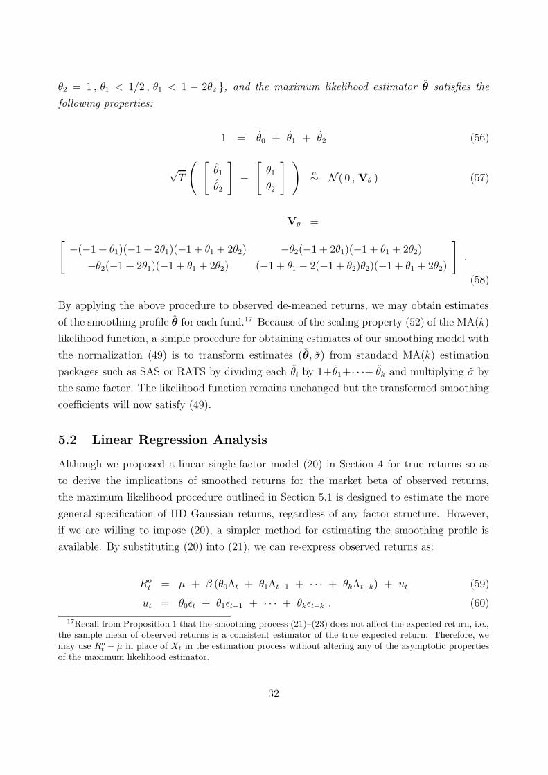
By applying the above procedure to observed de-meaned returns, we may obtain estimates

of the smoothing profile θ for each fund.17 Because of the scaling property (52) of the MA(k)

likelihood function, a simple procedure for obtaining estimates of our smoothing model with

the normalization (49) is to transform estimates (θ, σ) from standard MA(k) estimation

packages such as SAS or RATS by dividing each θi by 1+θ1+· · ·+ θk and multiplying σ by

the same factor. The likelihood function remains unchanged but the transformed smoothing

coefficients will now satisfy (49).

5.2 Linear Regression Analysis

Although we proposed a linear single-factor model (20) in Section 4 for true returns so as

to derive the implications of smoothed returns for the market beta of observed returns,

the maximum likelihood procedure outlined in Section 5.1 is designed to estimate the more

general specification of IID Gaussian returns, regardless of any factor structure. However,

if we are willing to impose (20), a simpler method for estimating the smoothing profile is

available. By substituting (20) into (21), we can re-express observed returns as:

Rot = µ + β (θ0Λt + θ1Λt−1 + · · · + θkΛt−k) + ut (59)

ut = θ0εt + θ1εt−1 + · · · + θkεt−k . (60)

17Recall from Proposition 1 that the smoothing process (21)–(23) does not affect the expected return, i.e.,the sample mean of observed returns is a consistent estimator of the true expected return. Therefore, wemay use Ro

t − µ in place of Xt in the estimation process without altering any of the asymptotic propertiesof the maximum likelihood estimator.

32

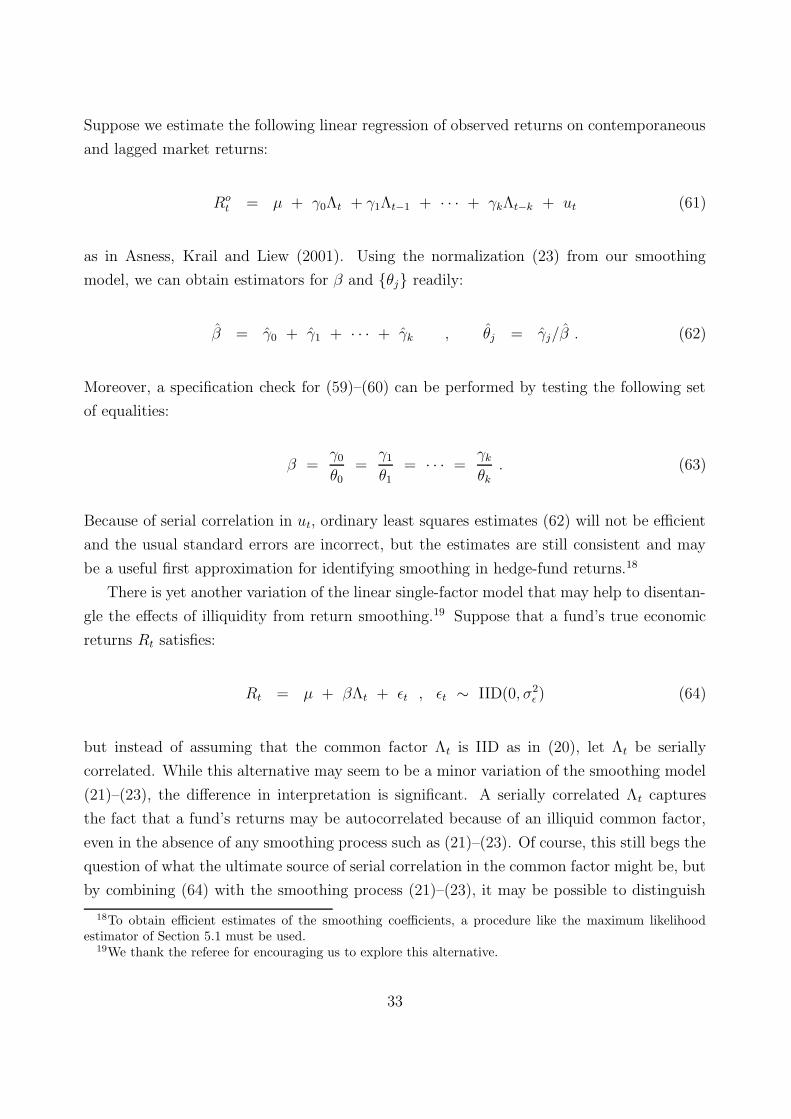
Suppose we estimate the following linear regression of observed returns on contemporaneous

and lagged market returns:

Rot = µ + γ0Λt + γ1Λt−1 + · · · + γkΛt−k + ut (61)

as in Asness, Krail and Liew (2001). Using the normalization (23) from our smoothing

model, we can obtain estimators for β and {θj} readily:

β = γ0 + γ1 + · · · + γk , θj = γj/β . (62)

Moreover, a specification check for (59)–(60) can be performed by testing the following set

of equalities:

β =γ0

θ0=

γ1

θ1= · · · =

γk

θk. (63)

Because of serial correlation in ut, ordinary least squares estimates (62) will not be efficient

and the usual standard errors are incorrect, but the estimates are still consistent and may

be a useful first approximation for identifying smoothing in hedge-fund returns.18

There is yet another variation of the linear single-factor model that may help to disentan-

gle the effects of illiquidity from return smoothing.19 Suppose that a fund’s true economic

returns Rt satisfies:

Rt = µ + βΛt + εt , εt ∼ IID(0, σ2ε ) (64)

but instead of assuming that the common factor Λt is IID as in (20), let Λt be serially

correlated. While this alternative may seem to be a minor variation of the smoothing model

(21)–(23), the difference in interpretation is significant. A serially correlated Λt captures

the fact that a fund’s returns may be autocorrelated because of an illiquid common factor,

even in the absence of any smoothing process such as (21)–(23). Of course, this still begs the

question of what the ultimate source of serial correlation in the common factor might be, but

by combining (64) with the smoothing process (21)–(23), it may be possible to distinguish

18To obtain efficient estimates of the smoothing coefficients, a procedure like the maximum likelihoodestimator of Section 5.1 must be used.

19We thank the referee for encouraging us to explore this alternative.

33

between “systematic” versus “idiosyncratic” smoothing, the former attributable to the asset

class and the latter resulting from fund-specific characteristics.

To see why the combination of (64) and (21)–(23) may have different implications for

observed returns, suppose for the moment that there is no smoothing, i.e., θ0 = 1 and θk = 0

for k > 0 in (21)–(23). Then observed returns are simply given by:

Rot = µ + βΛt + εt , εt ∼ IID(0, σ2

ε ) (65)

where Rot is now serially correlated solely through Λt. This specification implies that the

ratios of observed-return autocovariances will be identical across all funds with the same

common factor:

Cov[Rot , R

ot−k]

Cov[Rot , R

ot−l]

=β Cov[Λt, Λt−k]

β Cov[Λt, Λt−l]=

Cov[Λt, Λt−k]

Cov[Λt, Λt−l]. (66)

Moreover, (64) implies that in the regression equation (61), the coefficients of the lagged

factor returns are zero and the error term is not serially correlated.

More generally, consider the combination of a serially correlated common factor (64)

and smoothed returns (21)–(23). This more general econometric model of observed returns

implies that the appropriate specification of the regression equation is:

Rot = µ + γ0Λt + γ1Λt−1 + · · · + γkΛt−k + ut (67)

ut = θ0εt + θ1εt−1 + · · · + θkεt−k , εt ∼ IID(0, σ2ε ) (68)

1 = θ0 + θ1 + · · · + θk . (69)

To the extent that serial correlation in Rot can be explained mainly by the common factor,

the lagged coefficient estimates of (67) will be statistically insignificant, the residuals will be

serially uncorrelated, and the ratios of autocovariance coefficients will be roughly constant

across funds with the same common factor. To the extent that the smoothing process (21)–

(23) is responsible for serial correlation in Rot , the lagged coefficient estimates of (67) will

be significant, the residuals will be serially correlated, and the ratios γj/θj will be roughly

the same for all j ≥ 0 and will be a consistent estimate of the factor loading or beta of the

fund’s true economic returns with respect to the factor Λt.

Perhaps the most difficult challenge in estimating (67)–(69) is to correctly identify the

common factor Λt. Unlike a simple market-model regression that is meant to estimate

34

the sensitivity of a fund’s returns to a broad-based market index, the ability to distinguish

between the effects of systematic illiquidity and idiosyncratic return smoothing via (67) relies

heavily on the correct specification of the common factor. Using a common factor in (67)

that is highly serially correlated but not exactly the right factor for a given fund may yield

misleading estimates for the degree of smoothing in that fund’s observed returns. Therefore,

the common factor Λt must be selected or constructed carefully to match the specific risk

exposures of the fund, and the parameter estimates of (67) must be interpreted cautiously and

with several specific alternative hypotheses at hand. In Section 6.4, we provide an empirical

example that highlights the pitfalls and opportunities of the common factor specification

(67)–(69).

5.3 Specification Checks

Although the maximum likelihood estimator proposed in Section 5.1 has some attractive

properties—it is consistent and asymptotically efficient under certain regularity conditions—

it may not perform well in small samples or when the underlying distribution of true returns

is not normal as hypothesized.20 Moreover, even if normality is satisfied and a sufficient

sample size is available, our proposed smoothing model (21)–(23) may simply not apply to

some of the funds in our sample. Therefore, it is important to have certain specification

checks in mind when interpreting the empirical results.

The most obvious specification check is whether or not the maximum likelihood estima-

tion procedure, which involves numerical optimization, converges. If not, this is one sign

that our model is misspecified, either because of non-normality or because the smoothing

process is inappropriate.

A second specification check is whether or not the estimated smoothing coefficients are

all positive in sign (we do not impose non-negative restrictions in our estimation procedure,

despite the fact that the specification does assume non-negativity). Estimated coefficients

that are negative and significant may be a sign that the constraint (49) is violated, which

suggests that a somewhat different smoothing model may apply.

A third specification check is to compare the smoothing-parameter estimates from the

maximum likelihood approach of Section 5.1 with the linear regression approach of Section

5.2. If the linear single-factor model (20) holds, the two sets of smoothing-parameter esti-

mates should be close. Of course, omitted factors could be a source of discrepancies between

20There is substantial evidence that financial asset returns are not normally distributed, but characterizedby skewness, leptokurtosis, and other non-gaussian properties (see, for example, Lo and MacKinlay, 1999).Given the dynamic nature of hedge-fund strategies, it would be even less plausible for their returns to benormally distributed.

35

the two sets of estimates, so this specification check must be interpreted cautiously and with

some auxiliary information about the economic motivation for the common factor Λt.

Finally, a more direct approach to testing the specification of (21)–(23) is to impose a

different identification condition than (49). Suppose that the standard deviation ση of true

returns was observable; then the smoothing parameters θ are identified, and a simple check

of the specification (21)–(23) is to see whether the estimated parameters θ sum to 1. Of

course, ση is not observable, but if we had an alternative estimator ση for ση, we can achieve

identification of the MA(k) process by imposing the restriction:

ση = ση (70)

instead of (49). If, under this normalization, the smoothing parameter estimates are signifi-

cantly different, this may be a sign of misspecification.

The efficacy of this specification check depends on the quality of ση. We propose to

construct such an estimator by exploiting the fact that the discrepancy between observed

and true returns becomes “small” for multiperiod returns as the number of periods grows.

Specifically, recall from (37) that:

(Ro1 + Ro

2 + · · ·+ RoT ) = (R1 + R2 + · · ·+ RT ) +

k−1∑

j=0

(R−j − RT−j)(1 −j∑

i=0

θi) (71)

1

TVar

[T∑

t=1

Rot

]= σ2

η +σ2

η

T

k−1∑

j=0

(1 −

j∑

i=0

θi

)(1 − 2

j∑

i=0

θi

)(72)

and under the specification (21)–(23), it is easy to show that the second term on the right

side of (72) vanishes as T increases without bound, hence:

limT→∞

1

TVar

[T∑

t=1

Rot

]= σ2

η . (73)

To estimate this normalized variance of multiperiod observed returns, we can apply Newey

and West’s (1987) estimator:

σ2η ≡ 1

T

T∑

1

(Rot − µ)2 +

2

T

m∑

j=1

(1 − j

m + 1

)( T∑

t=j+1

(Rot − µ)(Ro

t−j − µ)

)(74)

36

where µ is the sample mean of {Rot} and m is a truncation lag that must increase with T

but at a slower rate to ensure consistency and asymptotic normality of the estimator. By

imposing the identification restriction

ση = ση (75)

in estimating the smoothing profile of observed returns, we obtain another estimator of θ

which can be compared against the first. As in the case of the normalization (49), the

alternate normalization (75) can be imposed by rescaling estimates (θ, σ) from standard

MA(k) estimation packages, in this case by dividing each θi by ση/σ and multiplying σ by

the same factor.

5.4 Smoothing-Adjusted Sharpe Ratios

One of the main implications of smoothed returns is that Sharpe ratios are biased upward, in

some cases substantially (see Proposition 1).21 The mechanism by which this bias occurs is

through the reduction in volatility because of the smoothing, but there is an additional bias

that occurs when monthly Sharpe ratios are annualized by multiplying by√

12. If monthly

returns are independently and identically distributed, this is the correct procedure, but Lo

(2002) shows that for non-IID returns, an alternative procedure must be used, one that

accounts for serial correlation in returns in a very specific manner.22 Specifically, denote by

Rt(q) the following q-period return:

Rt(q) ≡ Rt + Rt−1 + · · · + Rt−q+1 (76)

where we ignore the effects of compounding for computational convenience.23 For IID re-

turns, the variance of Rt(q) is directly proportional to q, hence the Sharpe ratio satisfies the

21There are a number of other concerns regarding the use and interpretation of Sharpe ratios in the contextof hedge funds. See Agarwal and Naik (2000a, 2002), Goetzmann et al. (2002), Lo (2001), Sharpe (1994),Spurgin (2001), and Weisman (2002) for examples where Sharpe ratios can be misleading indicators of thetrue risk-adjusted performance of hedge-fund strategies, and for alternate methods of constructing optimalportfolios of hedge funds.

22See also Jobson and Korkie (1981), who were perhaps the first to derive rigorous statistical propertiesof performance measures such as the Sharpe ratio and the Treynor measure.

23The exact expression is, of course:

Rt(q) ≡q−1∏

j=0

(1 + Rt−j) − 1 .

37

simple relation:

SR(q) =E[Rt(q)] − Rf(q)√

Var[Rt(q)]=

q(µ − Rf )√q σ

=√

q SR . (77)

Using Hansen’s (1982) GMM estimator, Lo (2002) derives the asymptotic distribution of

SR(q) as:

√T (SR(q) −√

q SR)a∼ N

(0 , VIID(q)

), VIID(q) = q VIID = q (1 + 1

2SR2) . (78)

For non-IID returns, the relation between SR and SR(q) is somewhat more involved

because the variance of Rt(q) is not just the sum of the variances of component returns, but

also includes all the covariances. Specifically, under the assumption that returns {Rt} are

stationary,

Var[Rt(q)] =

q−1∑

i=0

q−1∑

j=0

Cov[Rt−i, Rt−j] = qσ2 + 2σ2

q−1∑

k=1

(q−k)ρk (79)

where ρk≡Cov[Rt, Rt−k]/Var[Rt]. This yields the following relation between SR and SR(q):

SR(q) = η(q) SR , η(q) ≡ q√q + 2

∑q−1k=1(q−k)ρk

. (80)

Note that (80) reduces to (77) if the autocorrelations {ρk} are zero, as in the case of IID

returns. However, for non-IID returns, the adjustment factor for time-aggregated Sharpe

ratios is generally not√

q but a function of the first q−1 autocorrelations of returns, which

is readily estimated from the sample autocorrelations of returns, hence:

SR(q) = η(q) SR , η(q) ≡ q√q + 2

∑q−1k=1(q−k)ρk

(81)

where ρk is the sample k-th order autocorrelation coefficient.

For most (but not all) applications, (76) is an excellent approximation. Alternatively, if Rt is defined to bethe continuously compounded return, i.e., Rt ≡ log(Pt/Pt−1) where Pt is the price or net asset value at timet, then (76) is exact.

38

Lo (2002) also derives the asymptotic distribution of (81) under fairly general assumptions

for the returns process (stationarity and ergodicity) using generalized method of moments.

However, in the context of hedge-fund returns, the usual asymptotic approximations may not

be satisfactory because of the small sample sizes that characterize hedge-fund data—a five-

year track record, which amounts to only 60 monthly observations, is considered quite a long

history in this fast-paced industry. Therefore, we derive an alternate asymptotic distribution

using the continuous-record asymptotics of Richardson and Stock (1989). Specifically, as the

sample size T increases without bound, let q grow as well so that the ratio converges to some

finite limit between 0 and 1:

limq,T→∞

q/T = τ ∈ (0, 1) . (82)

This condition is meant to provide an asymptotic approximation that may be more accurate

for small-sample situations, i.e., situations where q is a significant fraction of T . For example,

in the case of a fund with a five-year track record, computing an annual Sharpe ratio with

monthly data corresponds to a value of 0.20 for the ratio q/T .

Now as q increases without bound, SR(q) also tends to infinity, hence we must renormalize

it to obtain a well-defined asymptotic sampling theory. In particular, observe that:

SR(q) =E[Rt(q)] − Rf (q)√

Var[Rt(q)]=

q(µ − Rf )√Var[Rt(q)]

(83)

SR(q)/√

q =µ − Rf√

Var[Rt(q)]/q(84)

limq→∞

SR(q)/√

q =µ − Rf

σ(85)

where σ can be viewed as a kind of long-run average return standard deviation, which is

generally not identical to the unconditional standard deviation σ of monthly returns except in

the IID case. To estimate σ, we can either follow Lo (2002) and use sample autocorrelations

as in (81), or estimate σ directly accordingly to Newey and West (1987):

σ2

NW ≡ 1

T

T∑

1

(Rt − µ)2 +2

T

m∑

j=1

(1 − j

m + 1)

T∑

t=j+1

(Rt − µ)(Rt−j − µ) (86)

where µ is the sample mean of {Rt}. For this estimator of σ, we have the following asymptotic

39

result:

Proposition 4 As m and T increase without bound so that m/T → λ ∈ (0, 1), σ2

NW con-

verges weakly to the following functional f(W ) of standard Brownian motion on [0, 1]:24

f(W ) ≡ 2σ2

λ

(∫ 1

0

W (r)[W (r) − W (min(r + λ, 1))

]dr −

W (1)

∫ λ

0

(λ − r)(W (1 − r) − W (r)

)dr +

λ(1 − λ2

3)

2W 2(1)

). (87)

From (87), a straightforward computation yields the following expectations:

E[σ2

NW] = 1 − λ +λ2

3, E[1/σNW] ≈

√1 + λ

1 − λ + λ2/3(88)

hence we propose the following bias-corrected estimator for the Sharpe ratio for small sam-

ples:

SR(q) =

√q(µ − Rf)

σNW

√1 − λ + λ3/2

1 + λ(89)

and its asymptotic distribution is given by the following proposition:

Proposition 5 As m, q, and T increase without bound so that m/T → λ ∈ (0, 1) and

q/T → τ ∈ (0, 1), the Sharpe ratio estimator SR(q) converges weakly to the following random

variable:

SR(q) ⇒(

SR(q)

f(W )+

√τW (1)

f(W )

) √1 − λ + λ3/2

1 + λ(90)

where f(W ) is given by (87), SR(q) is given by (83) and W (·) is standard Brownian motion

defined on [0, 1].

Monte Carlo simulations show that the second term of (90) does not account for much bias

when τ ∈ (0, 12], and that (90) is an excellent approximation to the small-sample distributions

of Sharpe ratios for non-IID returns.25

24See Billingsley (1968) for the definition of weak convergence and related results.25We have tabulated the percentiles of the distribution of (90) by Monte Carlo simulation for an extensive

40

6 Empirical Analysis

For our empirical analysis, we use the TASS database of hedge funds which consists of

monthly returns and accompanying information for 2,439 hedge funds (as of January 2001)

from November 1977 to January 2001.26 The database is divided into two parts: “Live”

and “Graveyard” funds. Hedge funds that belong to the Live database are considered to

be active as of January 1, 2001; once a hedge fund decides not to report its performance,

is liquidated, restructured, or merged with other hedge funds, the fund is transferred into

the Graveyard database. A hedge fund can only be listed in the Graveyard database after

being listed in the Live database, but the TASS database is subject to backfill bias—when

a fund decides to be included in the database, TASS adds the fund to the Live database

and includes available prior performance of the fund(hedge funds do not need to meet any

specific requirements to be included in the TASS database). Due to reporting delays and

time lags in contacting hedge funds, some Graveyard funds can be incorrectly listed in the

Live database for a period of time. However, TASS has adopted a policy of transferring funds

from the Live to the Graveyard database if they do not report over a 6–8 month period.

As of January 1, 2001, the combined data set of both live and dead hedge funds contained

2,439 funds with at least one monthly net return observation. Out of these 2,439 funds, 1,512

are in the Live database and 927 are in the Graveyard database. The earliest data available

for a fund in either database is November 1, 1977. The Graveyard database became active

only in 1994, i.e., funds that were dropped from the Live database prior to 1994 are not

included in the Graveyard database, which may yield a certain degree of survivorship bias.27

A majority of the 2,439 funds reported returns net of various fees on a monthly basis.28

We eliminated 30 funds that reported only gross returns and/or quarterly returns (15 from

each of the Live and Graveyard databases, respectively), leaving 2,409 funds in our sample.

We imposed an additional filter of including only those funds with at least five years of data,

leaving 651 funds in the Live database and 258 in the Graveyard database for a combined

combination of values of q, τ , and λ and would be happy to provide them to interested readers upon request.26For further information about the database and TASS, see http://www.tassresearch.com.27 For studies attempting to quantify the degree and impact of survivorship bias, see Baquero, Horst, and

Verbeek (2002), Brown, Goetzmann, Ibbotson, and Ross (1992), Brown, Goetzmann, and Ibbotson (1999),Brown, Goetzmann, and Park (1997), Carpenter and Lynch (1999), Fung and Hsieh (1997b, 2000), Horst,Nijman, T. and M. Verbeek (2001), Hendricks, Patel, and Zeckhauser (1997), and Schneeweis and Spurgin(1996).

28TASS defines returns as the change in net asset value during the month (assuming the reinvestment of anydistributions on the reinvestment date used by the fund) divided by the net asset value at the beginning of themonth, net of management fees, incentive fees, and other fund expenses. Therefore, these reported returnsshould approximate the returns realized by investors. TASS also converts all foreign-currency denominatedreturns to US-dollar returns using the appropriate exchange rates.

41

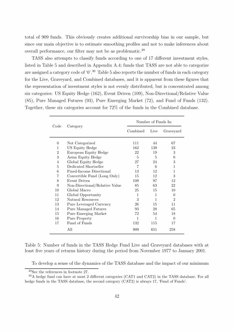
total of 909 funds. This obviously creates additional survivorship bias in our sample, but

since our main objective is to estimate smoothing profiles and not to make inferences about

overall performance, our filter may not be as problematic.29

TASS also attempts to classify funds according to one of 17 different investment styles,

listed in Table 5 and described in Appendix A.4; funds that TASS are not able to categorize

are assigned a category code of ‘0’.30 Table 5 also reports the number of funds in each category

for the Live, Graveyard, and Combined databases, and it is apparent from these figures that

the representation of investment styles is not evenly distributed, but is concentrated among

six categories: US Equity Hedge (162), Event Driven (109), Non-Directional/Relative Value

(85), Pure Managed Futures (93), Pure Emerging Market (72), and Fund of Funds (132).

Together, these six categories account for 72% of the funds in the Combined database.

Code CategoryNumber of Funds In:

Combined Live Graveyard

0 Not Categorized 111 44 671 US Equity Hedge 162 139 232 European Equity Hedge 22 19 33 Asian Equity Hedge 5 5 04 Global Equity Hedge 27 24 35 Dedicated Shortseller 7 6 16 Fixed-Income Directional 13 12 17 Convertible Fund (Long Only) 15 12 38 Event Driven 109 97 129 Non-Directional/Relative Value 85 63 22

10 Global Macro 25 15 1011 Global Opportunity 1 1 012 Natural Resources 3 1 213 Pure Leveraged Currency 26 15 1114 Pure Managed Futures 93 28 6515 Pure Emerging Market 72 54 1816 Pure Property 1 1 017 Fund of Funds 132 115 17

All 909 651 258

Table 5: Number of funds in the TASS Hedge Fund Live and Graveyard databases with atleast five years of returns history during the period from November 1977 to January 2001.

To develop a sense of the dynamics of the TASS database and the impact of our minimum

29See the references in footnote 27.30A hedge fund can have at most 2 different categories (CAT1 and CAT2) in the TASS database. For all

hedge funds in the TASS database, the second category (CAT2) is always 17, ‘Fund of Funds’.

42

return-history filter, in Table 6 we report annual frequency counts of the funds in the database

at the start of each year, funds entering during the year, funds exiting during the year, and

funds entering and exiting within the year. The left panel contains counts for the entire

TASS database, and the right panel contains counts for our sample of 909 funds with at

least five years of returns. The left panel shows that despite the start date of November

1977, the database is relatively sparsely populated until the 1990’s, with the largest increase

in new funds in 1998 and, in the aftermath of the collapse of LTCM, the largest number

of funds exiting the database in 1999 and 2000. The right panel of Table 6 illustrates the

impact of our five-year filter—the number of funds is considerably smaller, and although the

impact of survivorship bias can be ameliorated by the use of Live and Graveyard funds, our

sample of 909 funds will not include any of the funds started in 1997 and later which is a

substantial proportion of the TASS database.

The attrition rates reported in Table 6 are defined as the ratio of funds exiting in a given

year to the number of existing funds at the start of the year. TASS began tracking the exits

of funds starting only in 1994 hence attrition rates could not be computed in prior years. For

the unfiltered sample of all funds, the average attrition rate from 1994–1999 is 9.11%, which

is very similar to the 8.54% attrition rate obtained by Liang (2001) for the same period. As

observed above, the attrition rate skyrocketed in 2000 in the wake of LTCM’s demise. In

the right panel of Table 6, we see smaller attrition rates—the average over the 1994–1999

period is only 3.81%—because of our five-year minimum return history filter; since many

hedge funds fail in their first three years, our filtered sample is likely to have a much lower

attrition rate by construction.

Figure 4 contains a visual depiction of the variation in sample sizes of our 909 funds.

The start and end dates of the return history for each fund are connected by a vertical line

and plotted in Figure 4 according to the primary category of the fund—Categories 0–7 in

the top panel and Categories 8–17 in the bottom panel. It is apparent from the increasing

density of the graphs as we move from the bottom to the top that the majority of funds in

our sample are relatively new.

In Section 6.1 we present summary statistics for the sample of hedge funds included

in our analysis. We implement the smoothing profile estimation procedures outlined in

Section 5 for each of the funds, and in Section 6.2 we summarize the results of the maximum

likelihood and linear regression estimation procedures for the entire sample of funds and

for each style category. Section 6.3 reports the results of cross-sectional regressions of the

estimated smoothing coefficients, and in Section 6.4 we consider idiosyncratic and systematic

effects of illiquidity and smoothing by estimating a linear factor model with smoothing for

all funds in one particular style category using a common factor appropriate for that style.

43

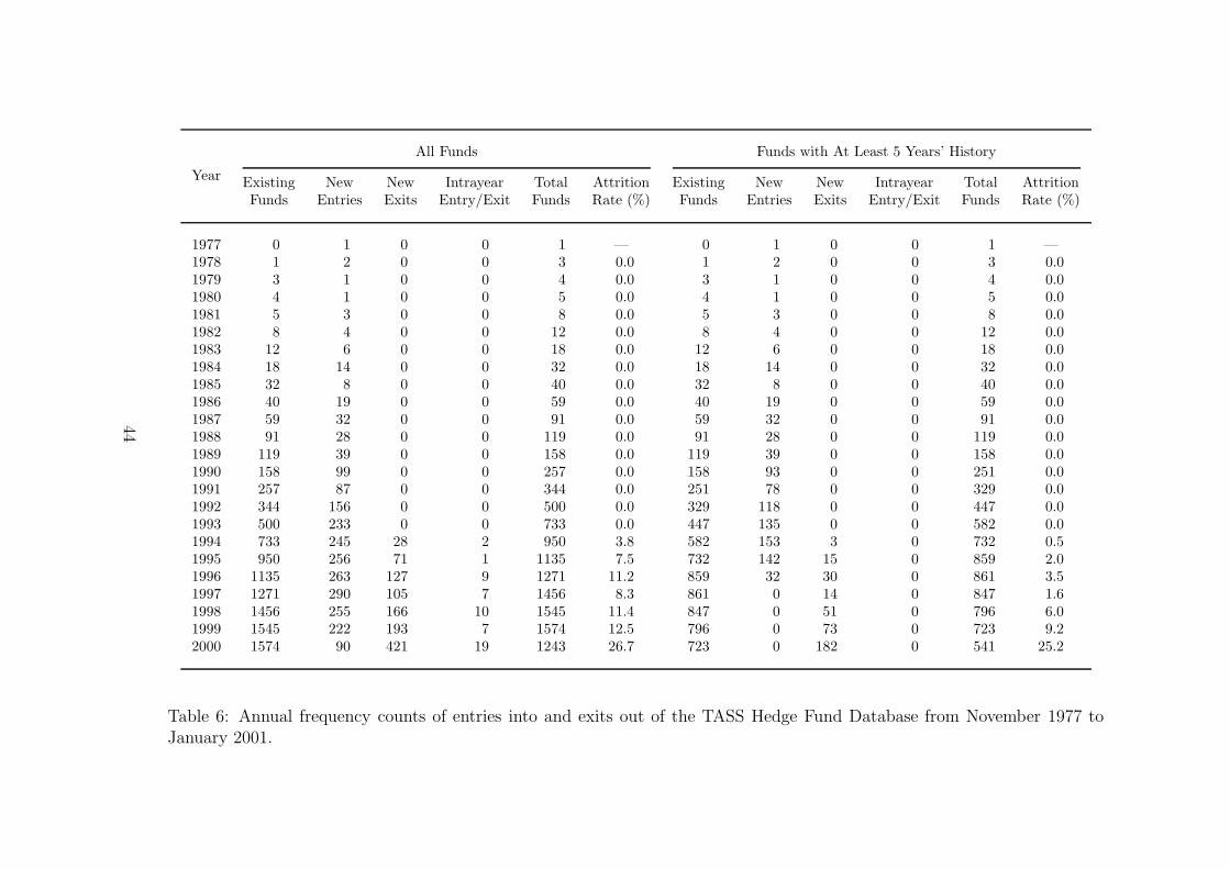
Year

All Funds Funds with At Least 5 Years’ History

Existing New New Intrayear Total Attrition Existing New New Intrayear Total AttritionFunds Entries Exits Entry/Exit Funds Rate (%) Funds Entries Exits Entry/Exit Funds Rate (%)

1977 0 1 0 0 1 — 0 1 0 0 1 —1978 1 2 0 0 3 0.0 1 2 0 0 3 0.01979 3 1 0 0 4 0.0 3 1 0 0 4 0.01980 4 1 0 0 5 0.0 4 1 0 0 5 0.01981 5 3 0 0 8 0.0 5 3 0 0 8 0.01982 8 4 0 0 12 0.0 8 4 0 0 12 0.01983 12 6 0 0 18 0.0 12 6 0 0 18 0.01984 18 14 0 0 32 0.0 18 14 0 0 32 0.01985 32 8 0 0 40 0.0 32 8 0 0 40 0.01986 40 19 0 0 59 0.0 40 19 0 0 59 0.01987 59 32 0 0 91 0.0 59 32 0 0 91 0.01988 91 28 0 0 119 0.0 91 28 0 0 119 0.01989 119 39 0 0 158 0.0 119 39 0 0 158 0.01990 158 99 0 0 257 0.0 158 93 0 0 251 0.01991 257 87 0 0 344 0.0 251 78 0 0 329 0.01992 344 156 0 0 500 0.0 329 118 0 0 447 0.01993 500 233 0 0 733 0.0 447 135 0 0 582 0.01994 733 245 28 2 950 3.8 582 153 3 0 732 0.51995 950 256 71 1 1135 7.5 732 142 15 0 859 2.01996 1135 263 127 9 1271 11.2 859 32 30 0 861 3.51997 1271 290 105 7 1456 8.3 861 0 14 0 847 1.61998 1456 255 166 10 1545 11.4 847 0 51 0 796 6.01999 1545 222 193 7 1574 12.5 796 0 73 0 723 9.22000 1574 90 421 19 1243 26.7 723 0 182 0 541 25.2

Table 6: Annual frequency counts of entries into and exits out of the TASS Hedge Fund Database from November 1977 toJanuary 2001.

44

And in Section 6.5 we summarize the properties of smoothing-adjusted Sharpe ratios for all

the funds in our sample and compare them to their unadjusted counterparts.

6.1 Summary Statistics

Table 7 contains basic summary statistics for the 909 funds in our combined extract from

the TASS Live and Graveyard databases. Not surprisingly, there is a great deal of varia-

tion in mean returns and volatilities both across and within categories. For example, the

162 US Equity Hedge funds in our sample exhibited a mean return of 22.53%, but with a

standard deviation of 10.80% in the cross section, and a mean volatility of 21.69% with a

cross-sectional standard deviation of 11.63%. Average serial correlations also vary consider-

ably across categories, but five categories stand out as having the highest averages:31 Fixed

Income Directional (21.6%), Convertible Fund (Long Only) (22.5%), Event Driven (20.8%),

Non-Directional/Relative Value (18.2%), and Pure Emerging Market (18.8%). Given the

descriptions of these categories provided by TASS (see Appendix A.4) and common wisdom

about the nature of the strategies involved—these categories include some of the most illiq-

uid securities traded—serial correlation seems to be a reasonable proxy for illiquidity and

smoothed returns. Alternatively, equities and futures are among the most liquid securities in

which hedge funds invest, and not surprising, the average first-order serial correlation for US

Equity Hedge funds and Pure Managed Futures is 7.8% and −0.1%, respectively. In fact, all

of the equity funds have average serial correlations that are much smaller than those of the

top five categories. Dedicated Shortseller funds also have a low average first-order autocor-

relation, 4.4%, which is consistent with the high degree of liquidity that often characterize

shortsellers (since, by definition, the ability to short a security implies a certain degree of

liquidity).

These summary statistics suggest that illiquidity and smoothed returns may be important

attributes for hedge-fund returns which can be captured to some degree by serial correlation

and our time-series model of smoothing.

6.2 Smoothing Profile Estimates

Using the methods outlined in Section 5, we estimate the smoothing model (21)–(23) and

summarize the results in Tables 8–9. Our maximum likelihood procedure—programmed in

Matlab using the Optimization Toolbox and replicated in Stata using its MA(k) estimation

31At 23.1% and −23.1%, respectively, Global Opportunity and Pure Property have higher first-orderautocorrelation coefficients in absolute value than the other categories, but since these two categories containonly a single fund each, we set them aside in our discussions.

45

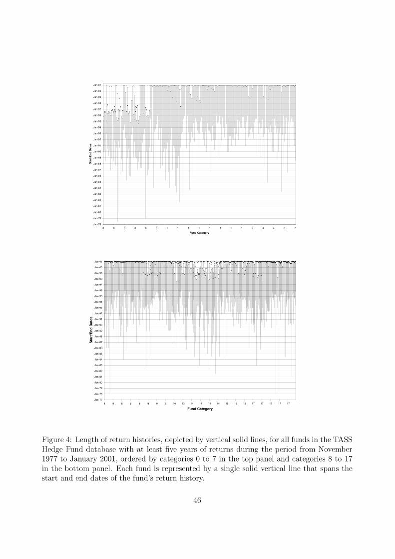
Jan-78

Jan-79

Jan-80

Jan-81

Jan-82

Jan-83

Jan-84

Jan-85

Jan-86

Jan-87

Jan-88

Jan-89

Jan-90

Jan-91

Jan-92

Jan-93

Jan-94

Jan-95

Jan-96

Jan-97

Jan-98

Jan-99

Jan-00

Jan-01

0 0 0 0 0 0 1 1 1 1 1 1 1 1 2 4 4 6 7

Fund Category

Sta

rt/E

nd D

ates

Jan-77

Jan-78

Jan-79

Jan-80

Jan-81

Jan-82

Jan-83

Jan-84

Jan-85

Jan-86

Jan-87

Jan-88

Jan-89

Jan-90

Jan-91

Jan-92

Jan-93

Jan-94

Jan-95

Jan-96

Jan-97

Jan-98

Jan-99

Jan-00

Jan-01

8 8 8 8 8 9 9 9 10 13 14 14 14 14 15 15 15 17 17 17 17 17

Fund�Category

Sta

rt/E

nd�D

ates

Figure 4: Length of return histories, depicted by vertical solid lines, for all funds in the TASSHedge Fund database with at least five years of returns during the period from November1977 to January 2001, ordered by categories 0 to 7 in the top panel and categories 8 to 17in the bottom panel. Each fund is represented by a single solid vertical line that spans thestart and end dates of the fund’s return history.

46

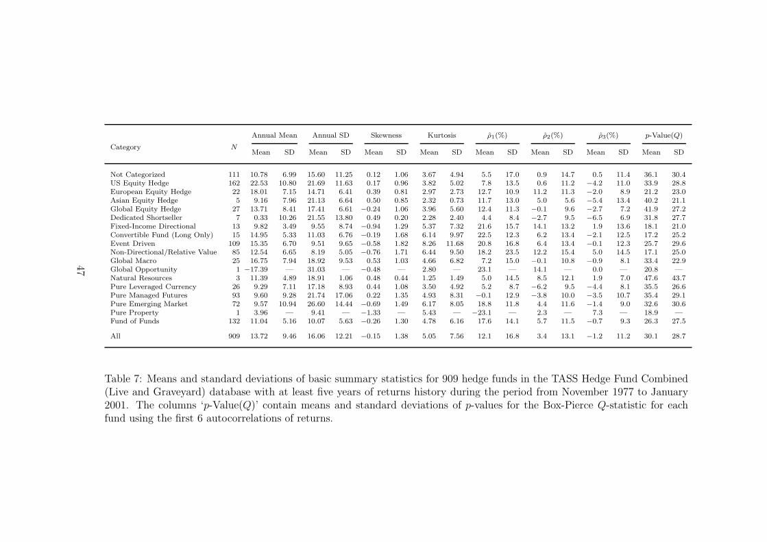
Category N

Annual Mean Annual SD Skewness Kurtosis ρ1(%) ρ2(%) ρ3(%) p-Value(Q)

Mean SD Mean SD Mean SD Mean SD Mean SD Mean SD Mean SD Mean SD

Not Categorized 111 10.78 6.99 15.60 11.25 0.12 1.06 3.67 4.94 5.5 17.0 0.9 14.7 0.5 11.4 36.1 30.4US Equity Hedge 162 22.53 10.80 21.69 11.63 0.17 0.96 3.82 5.02 7.8 13.5 0.6 11.2 −4.2 11.0 33.9 28.8European Equity Hedge 22 18.01 7.15 14.71 6.41 0.39 0.81 2.97 2.73 12.7 10.9 11.2 11.3 −2.0 8.9 21.2 23.0Asian Equity Hedge 5 9.16 7.96 21.13 6.64 0.50 0.85 2.32 0.73 11.7 13.0 5.0 5.6 −5.4 13.4 40.2 21.1Global Equity Hedge 27 13.71 8.41 17.41 6.61 −0.24 1.06 3.96 5.60 12.4 11.3 −0.1 9.6 −2.7 7.2 41.9 27.2Dedicated Shortseller 7 0.33 10.26 21.55 13.80 0.49 0.20 2.28 2.40 4.4 8.4 −2.7 9.5 −6.5 6.9 31.8 27.7Fixed-Income Directional 13 9.82 3.49 9.55 8.74 −0.94 1.29 5.37 7.32 21.6 15.7 14.1 13.2 1.9 13.6 18.1 21.0Convertible Fund (Long Only) 15 14.95 5.33 11.03 6.76 −0.19 1.68 6.14 9.97 22.5 12.3 6.2 13.4 −2.1 12.5 17.2 25.2Event Driven 109 15.35 6.70 9.51 9.65 −0.58 1.82 8.26 11.68 20.8 16.8 6.4 13.4 −0.1 12.3 25.7 29.6Non-Directional/Relative Value 85 12.54 6.65 8.19 5.05 −0.76 1.71 6.44 9.50 18.2 23.5 12.2 15.4 5.0 14.5 17.1 25.0Global Macro 25 16.75 7.94 18.92 9.53 0.53 1.03 4.66 6.82 7.2 15.0 −0.1 10.8 −0.9 8.1 33.4 22.9Global Opportunity 1 −17.39 — 31.03 — −0.48 — 2.80 — 23.1 — 14.1 — 0.0 — 20.8 —Natural Resources 3 11.39 4.89 18.91 1.06 0.48 0.44 1.25 1.49 5.0 14.5 8.5 12.1 1.9 7.0 47.6 43.7Pure Leveraged Currency 26 9.29 7.11 17.18 8.93 0.44 1.08 3.50 4.92 5.2 8.7 −6.2 9.5 −4.4 8.1 35.5 26.6Pure Managed Futures 93 9.60 9.28 21.74 17.06 0.22 1.35 4.93 8.31 −0.1 12.9 −3.8 10.0 −3.5 10.7 35.4 29.1Pure Emerging Market 72 9.57 10.94 26.60 14.44 −0.69 1.49 6.17 8.05 18.8 11.8 4.4 11.6 −1.4 9.0 32.6 30.6Pure Property 1 3.96 — 9.41 — −1.33 — 5.43 — −23.1 — 2.3 — 7.3 — 18.9 —Fund of Funds 132 11.04 5.16 10.07 5.63 −0.26 1.30 4.78 6.16 17.6 14.1 5.7 11.5 −0.7 9.3 26.3 27.5

All 909 13.72 9.46 16.06 12.21 −0.15 1.38 5.05 7.56 12.1 16.8 3.4 13.1 −1.2 11.2 30.1 28.7

Table 7: Means and standard deviations of basic summary statistics for 909 hedge funds in the TASS Hedge Fund Combined(Live and Graveyard) database with at least five years of returns history during the period from November 1977 to January2001. The columns ‘p-Value(Q)’ contain means and standard deviations of p-values for the Box-Pierce Q-statistic for eachfund using the first 6 autocorrelations of returns.

47

routine—converged without difficulty for all but one of the 909 funds:32 fund 1055, a Global

Macro fund with returns from June 1994 to January 2001 for which the maximum likelihood

estimation procedure yielded the following parameter estimates:

θ0 = 490.47 , θ1 = −352.63 , θ2 = −136.83

which suggests that our MA(2) model is severely misspecified for this fund. Therefore, we

drop this fund from our sample and for the remainder of our analysis, we focus on the

smoothing profile estimates for the remaining 908 funds in our sample.33

Table 8 contains summary statistics for maximum likelihood estimate of the smoothing

parameters (θ0, θ1, θ2) and smoothing index ξ, Table 12 reports comparable statistics for

the regression estimates of the smoothing parameters under the assumption of a linear one-

factor model for true returns, and Table 9 presents the maximum likelihood estimates of the

smoothing model for the 50 most illiquid funds of the 908 funds, as ranked by θ0.

The left panel of Table 8 reports summary statistics for the maximum likelihood estimates

under the normalization (49) where the smoothing coefficients sum to 1, and the right panel

reports the same statistics for the maximum likelihood estimates under the normalization

(75) where the variance σ2η is set equal to a nonparametric estimate σ2

η given by (74). A

comparison of the right and left panels reveals roughly similar characteristics, indicating the

general equivalence of these two normalization methods and the fact that the smoothing

model (21)–(23) may be a reasonable specification for hedge-fund returns.34

Table 8 shows that seven categories seem to exhibit smaller average values of θ0 than

the rest—European Equity Hedge (0.82), Fixed-Income Directional (0.76), Convertible Fund

(Long Only) (0.84), Event Driven (0.81), Non-Directional/Relative Value (0.82), Pure Emerg-

32We also constrain our maximum likelihood estimators to yield invertible MA(2) processes, and thisconstraint was binding for only two funds: 1711 and 4298.

33The apparent source of the problem in this case is two consecutive outliers, 39.4% in December 1999followed by −27.6% in January 2000 (these are monthly returns, not annualized). The effect of two outlierson the parameter estimates of the MA(2) model (21)–(23) is to pull the values of the coefficients in oppositedirections so as to fit the extreme reversals. We contacted TASS to investigate these outliers and wereinformed that they were data errors. We also checked the remaining 908 funds in our sample for similaroutliers, i.e., consecutive extreme returns of opposite sign, and found none. We also computed the maximumand minimum monthly returns for each fund in our sample, ranked the 908 funds according to these maximaand minima, and checked the parameter estimates of the top and bottom 10 funds, and none exhibited theextreme behavior of fund 1055’s parameter estimates.

34However, Table 8 contains only summary statistics, not the maximum likelihood estimators of individualfunds, hence differences in the two normalizations for given funds may not be apparent from this table. Inparticular, side-by-side comparisons of maximum likelihood estimates for an individual under these two nor-malizations may still be a useful specification check despite the broad similarities that these two approachesseem to exhibit in Table 8.

48

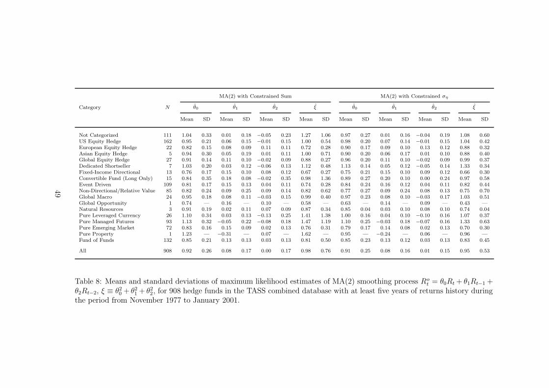
Category N

MA(2) with Constrained Sum MA(2) with Constrained ση

θ0 θ1 θ2 ξ θ0 θ1 θ2 ξ

Mean SD Mean SD Mean SD Mean SD Mean SD Mean SD Mean SD Mean SD

Not Categorized 111 1.04 0.33 0.01 0.18 −0.05 0.23 1.27 1.06 0.97 0.27 0.01 0.16 −0.04 0.19 1.08 0.60US Equity Hedge 162 0.95 0.21 0.06 0.15 −0.01 0.15 1.00 0.54 0.98 0.20 0.07 0.14 −0.01 0.15 1.04 0.42European Equity Hedge 22 0.82 0.15 0.08 0.09 0.11 0.11 0.72 0.28 0.90 0.17 0.09 0.10 0.13 0.12 0.88 0.32Asian Equity Hedge 5 0.94 0.30 0.05 0.19 0.01 0.11 1.00 0.71 0.90 0.20 0.06 0.17 0.01 0.10 0.88 0.40Global Equity Hedge 27 0.91 0.14 0.11 0.10 −0.02 0.09 0.88 0.27 0.96 0.20 0.11 0.10 −0.02 0.09 0.99 0.37Dedicated Shortseller 7 1.03 0.20 0.03 0.12 −0.06 0.13 1.12 0.48 1.13 0.14 0.05 0.12 −0.05 0.14 1.33 0.34Fixed-Income Directional 13 0.76 0.17 0.15 0.10 0.08 0.12 0.67 0.27 0.75 0.21 0.15 0.10 0.09 0.12 0.66 0.30Convertible Fund (Long Only) 15 0.84 0.35 0.18 0.08 −0.02 0.35 0.98 1.36 0.89 0.27 0.20 0.10 0.00 0.24 0.97 0.58Event Driven 109 0.81 0.17 0.15 0.13 0.04 0.11 0.74 0.28 0.84 0.24 0.16 0.12 0.04 0.11 0.82 0.44Non-Directional/Relative Value 85 0.82 0.24 0.09 0.25 0.09 0.14 0.82 0.62 0.77 0.27 0.09 0.24 0.08 0.13 0.75 0.70Global Macro 24 0.95 0.18 0.08 0.11 −0.03 0.15 0.99 0.40 0.97 0.23 0.08 0.10 −0.03 0.17 1.03 0.51Global Opportunity 1 0.74 — 0.16 — 0.10 — 0.58 — 0.63 — 0.14 — 0.09 — 0.43 —Natural Resources 3 0.91 0.19 0.02 0.11 0.07 0.09 0.87 0.34 0.85 0.04 0.03 0.10 0.08 0.10 0.74 0.04Pure Leveraged Currency 26 1.10 0.34 0.03 0.13 −0.13 0.25 1.41 1.38 1.00 0.16 0.04 0.10 −0.10 0.16 1.07 0.37Pure Managed Futures 93 1.13 0.32 −0.05 0.22 −0.08 0.18 1.47 1.19 1.10 0.25 −0.03 0.18 −0.07 0.16 1.33 0.63Pure Emerging Market 72 0.83 0.16 0.15 0.09 0.02 0.13 0.76 0.31 0.79 0.17 0.14 0.08 0.02 0.13 0.70 0.30Pure Property 1 1.23 — −0.31 — 0.07 — 1.62 — 0.95 — −0.24 — 0.06 — 0.96 —Fund of Funds 132 0.85 0.21 0.13 0.13 0.03 0.13 0.81 0.50 0.85 0.23 0.13 0.12 0.03 0.13 0.83 0.45

All 908 0.92 0.26 0.08 0.17 0.00 0.17 0.98 0.76 0.91 0.25 0.08 0.16 0.01 0.15 0.95 0.53

Table 8: Means and standard deviations of maximum likelihood estimates of MA(2) smoothing process Rot = θ0Rt + θ1Rt−1 +

θ2Rt−2, ξ ≡ θ20 + θ2

1 + θ22, for 908 hedge funds in the TASS combined database with at least five years of returns history during

the period from November 1977 to January 2001.

49

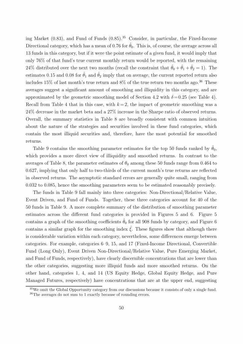
ing Market (0.83), and Fund of Funds (0.85).35 Consider, in particular, the Fixed-Income

Directional category, which has a mean of 0.76 for θ0. This is, of course, the average across all

13 funds in this category, but if it were the point estimate of a given fund, it would imply that

only 76% of that fund’s true current monthly return would be reported, with the remaining

24% distributed over the next two months (recall the constraint that θ0 + θ1 + θ2 = 1). The

estimates 0.15 and 0.08 for θ1 and θ2 imply that on average, the current reported return also

includes 15% of last month’s true return and 8% of the true return two months ago.36 These

averages suggest a significant amount of smoothing and illiquidity in this category, and are

approximated by the geometric smoothing model of Section 4.2 with δ=0.25 (see Table 4).

Recall from Table 4 that in this case, with k =2, the impact of geometric smoothing was a

24% decrease in the market beta and a 27% increase in the Sharpe ratio of observed returns.

Overall, the summary statistics in Table 8 are broadly consistent with common intuition

about the nature of the strategies and securities involved in these fund categories, which

contain the most illiquid securities and, therefore, have the most potential for smoothed

returns.

Table 9 contains the smoothing parameter estimates for the top 50 funds ranked by θ0,

which provides a more direct view of illiquidity and smoothed returns. In contrast to the

averages of Table 8, the parameter estimates of θ0 among these 50 funds range from 0.464 to

0.627, implying that only half to two-thirds of the current month’s true returns are reflected

in observed returns. The asymptotic standard errors are generally quite small, ranging from

0.032 to 0.085, hence the smoothing parameters seem to be estimated reasonably precisely.

The funds in Table 9 fall mainly into three categories: Non-Directional/Relative Value,

Event Driven, and Fund of Funds. Together, these three categories account for 40 of the

50 funds in Table 9. A more complete summary of the distribution of smoothing parameter

estimates across the different fund categories is provided in Figures 5 and 6. Figure 5

contains a graph of the smoothing coefficients θ0 for all 908 funds by category, and Figure 6

contains a similar graph for the smoothing index ξ. These figures show that although there

is considerable variation within each category, nevertheless, some differences emerge between

categories. For example, categories 6–9, 15, and 17 (Fixed-Income Directional, Convertible

Fund (Long Only), Event Driven Non-Directional/Relative Value, Pure Emerging Market,

and Fund of Funds, respectively), have clearly discernible concentrations that are lower than

the other categories, suggesting more illiquid funds and more smoothed returns. On the

other hand, categories 1, 4, and 14 (US Equity Hedge, Global Equity Hedge, and Pure

Managed Futures, respectively) have concentrations that are at the upper end, suggesting

35We omit the Global Opportunity category from our discussions because it consists of only a single fund.36The averages do not sum to 1 exactly because of rounding errors.

50

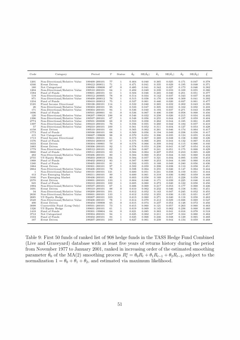
Code Category Period T Status θ0 SE(θ0) θ1 SE(θ1) θ2 SE(θ2) ξ

1201 Non-Directional/Relative Value 199409–200101 77 1 0.464 0.040 0.365 0.025 0.171 0.047 0.3784346 Event Driven 199412–200011 71 1 0.471 0.041 0.335 0.029 0.195 0.048 0.371180 Not Categorized 198906–199608 87 0 0.485 0.041 0.342 0.027 0.173 0.046 0.382

1204 Non-Directional/Relative Value 199510–200101 64 1 0.492 0.049 0.339 0.033 0.169 0.055 0.3861584 Fund of Funds 199601–200101 61 1 0.504 0.046 0.245 0.040 0.251 0.051 0.377518 Non-Directional/Relative Value 199312–200005 78 0 0.514 0.034 0.142 0.037 0.343 0.037 0.403971 Non-Directional/Relative Value 199409–200012 76 1 0.515 0.038 0.176 0.038 0.309 0.041 0.392

1234 Fund of Funds 199410–200012 75 1 0.527 0.061 0.446 0.020 0.027 0.061 0.4772185 Fixed Income Directional 199108–200101 114 1 0.532 0.040 0.265 0.032 0.202 0.043 0.395

26 Non-Directional/Relative Value 199303–200101 95 1 0.533 0.047 0.305 0.033 0.162 0.050 0.403171 Non-Directional/Relative Value 199304–200101 94 1 0.536 0.040 0.193 0.037 0.271 0.043 0.398

1696 Fund of Funds 199501–200001 61 0 0.536 0.067 0.406 0.030 0.058 0.068 0.456120 Non-Directional/Relative Value 198207–199810 196 0 0.546 0.032 0.238 0.026 0.215 0.034 0.402

1396 Non-Directional/Relative Value 199507–200101 67 1 0.548 0.056 0.255 0.044 0.197 0.059 0.4042774 Non-Directional/Relative Value 199501–200006 66 0 0.553 0.058 0.262 0.044 0.185 0.061 0.4091397 Non-Directional/Relative Value 199410–200101 76 1 0.556 0.055 0.260 0.042 0.184 0.057 0.410

57 Non-Directional/Relative Value 199210–200101 100 1 0.561 0.052 0.311 0.034 0.127 0.053 0.4284158 Event Driven 199510–200101 64 1 0.565 0.062 0.261 0.046 0.174 0.064 0.4171773 Fund of Funds 199506–200101 68 1 0.569 0.056 0.194 0.049 0.238 0.058 0.417415 Not Categorized 198807–199608 98 0 0.570 0.054 0.306 0.035 0.124 0.055 0.434

1713 Fixed Income Directional 199601–200101 61 1 0.573 0.067 0.269 0.048 0.158 0.068 0.4261576 Fund of Funds 199504–200010 67 1 0.575 0.066 0.293 0.044 0.132 0.067 0.4341633 Event Driven 199304–199901 70 0 0.576 0.066 0.309 0.042 0.115 0.066 0.4401883 Event Driven 199306–200101 92 1 0.578 0.053 0.236 0.041 0.187 0.054 0.4241779 Non-Directional/Relative Value 199512–200101 62 1 0.584 0.067 0.241 0.051 0.175 0.068 0.4293860 Fund of Funds 199511–200101 63 1 0.584 0.064 0.207 0.053 0.210 0.065 0.428482 Non-Directional/Relative Value 199406–200101 80 1 0.584 0.060 0.253 0.044 0.163 0.060 0.432

2755 US Equity Hedge 199203–200010 104 1 0.584 0.057 0.321 0.034 0.095 0.056 0.4531968 Fund of Funds 199402–200012 83 1 0.587 0.060 0.253 0.044 0.160 0.060 0.4341240 Fund of Funds 199405–200101 81 1 0.592 0.055 0.168 0.049 0.240 0.056 0.4361884 Event Driven 199301–200101 97 1 0.592 0.059 0.298 0.038 0.110 0.058 0.4512864 Non-Directional/Relative Value 199408–200101 78 1 0.598 0.064 0.255 0.046 0.147 0.064 0.444

1 Non-Directional/Relative Value 199101–200101 121 1 0.600 0.051 0.241 0.038 0.159 0.051 0.444412 Pure Emerging Market 199211–200101 99 1 0.600 0.061 0.318 0.036 0.082 0.059 0.468

1046 Pure Emerging Market 199406–200101 80 1 0.603 0.058 0.169 0.051 0.228 0.058 0.4442570 Event Driven 199001–200101 133 1 0.604 0.046 0.171 0.039 0.225 0.046 0.445945 Fund of Funds 199210–200101 100 1 0.605 0.060 0.273 0.040 0.122 0.058 0.456

1994 Non-Directional/Relative Value 199507–200101 67 1 0.606 0.069 0.217 0.053 0.177 0.068 0.4461691 Event Driven 199310–200101 88 0 0.610 0.062 0.232 0.046 0.158 0.061 0.451

34 Non-Directional/Relative Value 199209–200101 101 1 0.612 0.052 0.143 0.047 0.245 0.052 0.4552630 Non-Directional/Relative Value 199001–200101 133 1 0.612 0.052 0.255 0.036 0.133 0.051 0.4572685 US Equity Hedge 199207–200101 103 1 0.613 0.060 0.271 0.040 0.116 0.058 0.4632549 Non-Directional/Relative Value 199408–200101 78 1 0.614 0.079 0.412 0.029 −0.026 0.069 0.547490 Event Driven 199404–199908 65 0 0.615 0.074 0.237 0.054 0.148 0.072 0.456

3099 Convertible Fund (Long Only) 199501–200101 73 1 0.615 0.060 0.121 0.057 0.263 0.060 0.4631326 US Equity Hedge 199601–200101 61 1 0.619 0.069 0.145 0.062 0.236 0.068 0.4601418 Fund of Funds 199301–199804 64 0 0.621 0.085 0.363 0.041 0.016 0.078 0.5183712 Not Categorized 199304–200101 94 1 0.625 0.062 0.211 0.047 0.164 0.060 0.4621534 Fund of Funds 199402–200101 84 1 0.625 0.068 0.246 0.048 0.129 0.065 0.468167 Event Driven 199207–200101 103 1 0.627 0.061 0.239 0.044 0.134 0.059 0.468

Table 9: First 50 funds of ranked list of 908 hedge funds in the TASS Hedge Fund Combined(Live and Graveyard) database with at least five years of returns history during the periodfrom November 1977 to January 2001, ranked in increasing order of the estimated smoothingparameter θ0 of the MA(2) smoothing process Ro

t = θ0Rt + θ1Rt−1 + θ2Rt−2, subject to thenormalization 1 = θ0 + θ1 + θ2, and estimated via maximum likelihood.

51

just the opposite—more liquidity and less return-smoothing. The smoothing index estimates

ξ plotted in Figure 6 show similar patterns of concentration and dispersion within and

between the categories.

To develop further intuition for the smoothing model (21)–(23) and the possible interpre-

tations of the smoothing parameter estimates, we apply the same estimation procedure to

the returns of the Ibbotson stock and bond indexes, the Merrill Lynch Convertible Securities

Index,37 the CSFB/Tremont hedge-fund indexes, and two mutual funds, the highly liquid

Vanguard 500 Index Fund, and the considerably less liquid American Express Extra Income

Fund.38 Table 10 contains summary statistics, market betas, contemporaneous and lagged

market betas as in Asness, Krail and Liew (2001), and smoothing-coefficient estimates for

these index and mutual-fund returns.39

Consistent with our interpretation of θ0 as an indicator of liquidity, the returns of the

most liquid portfolios in the first panel of Table 10—the Ibbotson Large Company Index, the

Vanguard 500 Index Fund (which is virtually identical to the Ibbotson Large Company Index,

except for sample period and tracking error), and the Ibbotson Long-Term Government

Bond Index—have smoothing parameter estimates near unity: 0.92 for the Ibbotson Large

Company Index, 1.12 for the Vanguard 500 Index Fund, and 0.92 for the Ibbotson Long-Term

Government Bond Index. The first-order autocorrelation coefficients and lagged market

betas also confirm their lack of serial correlation; 9.8% first-order autocorrelation for the

Ibbotson Large Company Index , −2.3% for the Vanguard 500 Index Fund, and 6.7% for the

Ibbotson Long-Term Government Bond Index, and lagged market betas that are statistically

indistinguishable from 0. However, the values of θ0 of the less liquid portfolios are less

37 This is described by Merrill Lynch as a “market value-weighted index that tracks the daily priceonly, income and total return performance of corporate convertible securities, including US domestic bonds,Eurobonds, preferred stocks and Liquid Yield Option Notes”.

38As of January 31, 2003, the net assets of the Vanguard 500 Index Fund (ticker symbol: VFINX) and theAXP Extra Income Fund (ticker symbol: INEAX) are given by http://finance.yahoo.com/ as $59.7 billionand $1.5 billion, respectively, and the descriptions of the two funds are as follows:

“The Vanguard 500 Index Fund seeks investment results that correspond with the price and yield per-formance of the S&P 500 Index. The fund employs a passive management strategy designed to track theperformance of the S&P 500 Index, which is dominated by the stocks of large U.S. companies. It attemptsto replicate the target index by investing all or substantially all of its assets in the stocks that make up theindex.”

“AXP Extra Income Fund seeks high current income; capital appreciation is secondary. The fund ordinarilyinvests in long-term high-yielding, lower-rated corporate bonds. These bonds may be issued by U.S. andforeign companies and governments. The fund may invest in other instruments such as: money marketsecurities, convertible securities, preferred stocks, derivatives (such as futures, options and forward contracts),and common stocks.”

39Market betas were obtained by regressing returns on a constant and the total return of the S&P 500,and contemporaneous and lagged market betas were obtained by regressing returns on a constant, thecontemporaneous total return of the S&P 500, and the first two lags.

52

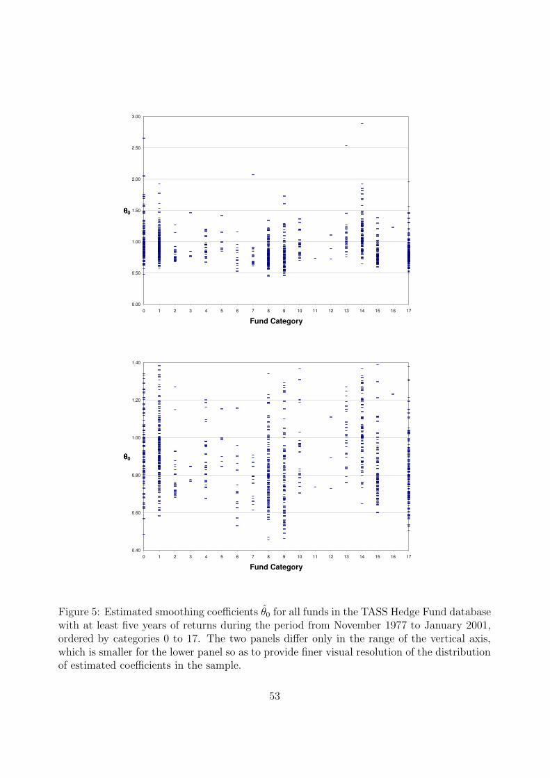
0.00

0.50

1.00

1.50

2.00

2.50

3.00

0 1 2 3 4 5 6 7 8 9 10 11 12 13 14 15 16 17

Fund�Category

θθθθ0

0.40

0.60

0.80

1.00

1.20

1.40

0 1 2 3 4 5 6 7 8 9 10 11 12 13 14 15 16 17

Fund�Category

θθθθ0

Figure 5: Estimated smoothing coefficients θ0 for all funds in the TASS Hedge Fund databasewith at least five years of returns during the period from November 1977 to January 2001,ordered by categories 0 to 17. The two panels differ only in the range of the vertical axis,which is smaller for the lower panel so as to provide finer visual resolution of the distributionof estimated coefficients in the sample.

53

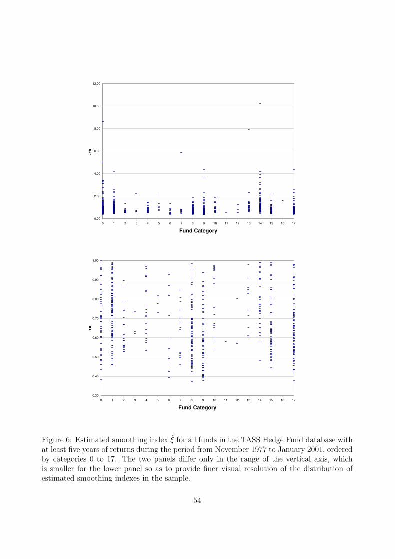
0.00

2.00

4.00

6.00

8.00

10.00

12.00

0 1 2 3 4 5 6 7 8 9 10 11 12 13 14 15 16 17

Fund�Category

ξξξξ

0.30

0.40

0.50

0.60

0.70

0.80

0.90

1.00

0 1 2 3 4 5 6 7 8 9 10 11 12 13 14 15 16 17

Fund�Category

ξξξξ

Figure 6: Estimated smoothing index ξ for all funds in the TASS Hedge Fund database withat least five years of returns during the period from November 1977 to January 2001, orderedby categories 0 to 17. The two panels differ only in the range of the vertical axis, whichis smaller for the lower panel so as to provide finer visual resolution of the distribution ofestimated smoothing indexes in the sample.

54

than 1.00: 0.82 for the Ibbotson Small Company Index, 0.84 for the Ibbotson Long-Term

Corporate Bond Index, 0.82 for the Merrill Lynch Convertible Securities Index, and 0.67 for

the American Express Extra Income Fund, and their first-order serial correlation coefficients

are 15.6%, 15.6%, 6.4% and 35.4%, respectively, which, with the exception of the Merrill

Lynch Convertible Securities Index, are considerably higher than those of the more liquid

portfolios.40 Also, the lagged market betas are statistically significant at the 5% level for

the Ibbotson Small Company Index (a t-statistic for β1: 5.41), the Ibbotson Long-Term

Government Bond Index (t-statistic for β1: −2.30), the Merrill Lynch Convertible Securities

Index (t-statistic for β1: 3.33), and the AXP Extra Income Fund (t-statistic for β1: 4.64).

The results for the CSFB Hedge Fund Indexes in the second panel of Table 10 are also

consistent with the empirical results in Tables 8 and 9—indexes corresponding to hedge-fund

strategies involving less liquid securities tend to have lower θ0’s. For example, the smoothing-

parameter estimates θ0 of the Convertible Arbitrage, Emerging Markets, and Fixed-Income

Arbitrage Indexes are 0.49, 0.75, and 0.63, respectively, and first-order serial correlation

coefficients of 56.6%, 29.4%, and 39.6%, respectively. In contrast, the smoothing-parameter

estimates of the more liquid hedge-fund strategies such as Dedicated Short Bias and Man-

aged Futures are 0.99 and 1.04, respectively, with first-order serial correlation coefficients of

7.8% and 3.2%, respectively. While these findings are generally consistent with the results

in Tables 8 and 9, it should be noted that the process of aggregation can change the sta-

tistical behavior of any time series. For example, Granger (1980, 1988) observes that the

aggregation of a large number of stationary autoregressive processes can yield a time series

that exhibits long-term memory, characterized by serial correlation coefficients that decay

very slowly (hyperbolically, as opposed to geometrically as in the case of a stationary ARMA

process). Therefore, while it is true that the aggregation of a collection of illiquid funds will

generally yield an index with smoothed returns,41 the reverse need not be true—smoothed

index returns need not imply that all of the funds comprising the index are illiquid. The

latter inference can only be made with the benefit of additional information—essentially

identification restrictions—about the statistical relations among the funds in the index, i.e.,

covariances and possibly other higher-order co-moments, or the existence of common factors

driving fund returns.

40However, note that the second-order autocorrelation of the Merrill Lynch Convertible Securities Index is12.0% which is second only to the AXP Extra Income Fund in absolute magnitude, two orders of magnitudelarger than the second-order autocorrelation of the Ibbotson bond indexes, and one order of magnitude largerthan the Ibbotson stock indexes.

41It is, of course, possible that the smoothing coefficients of some funds may exactly offset those of otherfunds so as to reduce the degree of smoothing in an aggregate index. However, such a possibility is extremelyremote and pathological if each of the component funds exhibits a high degree of smoothing.

55

It is interesting to note that the first lagged market beta, β1, for the CSFB/Tremont

Indexes is statistically significant at the 5% level in only three cases (Convertible Arbitrage,

Event Driven, and Managed Futures), but the second lagged beta, β2, is significant in five

cases (the overall index, Convertible Arbitrage, Fixed Income Arbitrage, Global Macro,

and Long/Short). Obviously, the S&P 500 Index is likely to be inappropriate for certain

styles, e.g., Emerging Markets, and these somewhat inconsistent results suggest that using

a lagged market-beta adjustment may not completely account for the impact of illiquidity

and smoothed returns.

Overall, the patterns in Table 10 confirm our interpretation of smoothing coefficients and

serial correlation as proxies for liquidity, and suggest that there may be broader applications

of our model of smoothed returns to other investment strategies and asset classes.

6.3 Cross-Sectional Regressions

A more quantitative summary of the cross-sectional properties of the smoothing parameter

estimates for the 908 funds is given in Table 11, which contains the results of cross-sectional

regressions of the smoothing parameter θ0 and the smoothing index ξ on a number of 0/1

indicator variables.42 In the first two regressions, θ0 and ξ are the dependent variables,

respectively, and the regressors include a constant term, 17 indicator variables corresponding

to the 17 hedge-fund categories defined by TASS (see Appendix A.4), and an indicator

variable that takes on the value 1 if the fund is open and 0 if it is closed to new investors. The

third and fourth regressions have the same dependent variables—θ0 and ξ, respectively—and

include the same regressors as the first two regressions but also include 0/1 indicator variables

that indicate whether the fund is US-based (USBASED), and whether the geographical focus

of the fund is global (GF-GLB), US (GF-USA), Asia/Pacific (GF-APC), Western Europe

(GF-WEU), Eastern Europe (GF-EEU), and Africa (GF-AFR).

The results of the first regression are consistent with the general intuition gleaned from

Figures 5 and 6. The category indicator variables with the most negative coefficients that are

statistically significant at the 5% level are European Equity Hedge (−0.212), Fixed-Income

Directional (−0.262), Event Driven (−0.218), Non-Directional/Relative Value (−0.211),

Pure Emerging Market (−0.195), Fund of Funds (−0.178), implying that on average, funds

in these categories have smaller smoothing coefficients θ0, i.e., less liquidity or smoother

returns. These point estimates can be used to approximate the marginal impact that a

42To conserve space, we report regression results only for the maximum likelihood estimates under the con-straint (49). Table A.8 of the Appendix reports corresponding results for the maximum likelihood estimatesunder the alternate constraint (75).

56

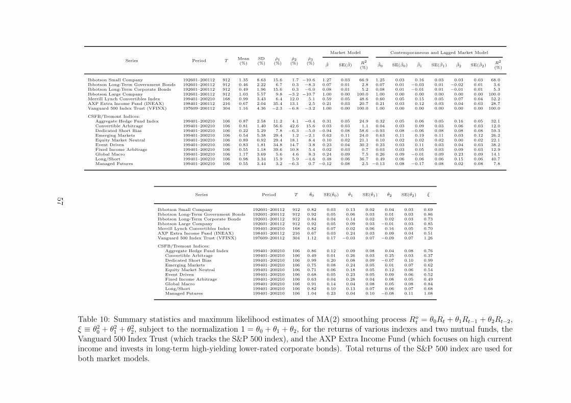
Market Model Contemporaneous and Lagged Market Model

Series Period TMean SD ρ1 ρ2 ρ3

β SE(β)R2

β0 SE(β0) β1 SE(β1) β2 SE(β2)R2

(%) (%) (%) (%) (%)(%) (%)

Ibbotson Small Company 192601–200112 912 1.35 8.63 15.6 1.7 −10.6 1.27 0.03 66.9 1.25 0.03 0.16 0.03 0.03 0.03 68.0Ibbotson Long-Term Government Bonds 192601–200112 912 0.46 2.22 6.7 0.3 −8.3 0.07 0.01 2.8 0.07 0.01 −0.03 0.01 −0.02 0.01 3.6Ibbotson Long-Term Corporate Bonds 192601–200112 912 0.49 1.96 15.6 0.3 −6.0 0.08 0.01 5.2 0.08 0.01 −0.01 0.01 −0.01 0.01 5.3Ibbotson Large Company 192601–200112 912 1.03 5.57 9.8 −3.2 −10.7 1.00 0.00 100.0 1.00 0.00 0.00 0.00 0.00 0.00 100.0Merrill Lynch Convertibles Index 199401–200210 168 0.99 3.43 6.4 12.0 5.1 0.59 0.05 48.6 0.60 0.05 0.15 0.05 0.07 0.04 52.2AXP Extra Income Fund (INEAX) 198401–200112 216 0.67 2.04 35.4 13.1 2.5 0.21 0.03 20.7 0.21 0.03 0.12 0.03 0.04 0.03 28.7Vanguard 500 Index Trust (VFINX) 197609–200112 304 1.16 4.36 −2.3 −6.8 −3.2 1.00 0.00 100.0 1.00 0.00 0.00 0.00 0.00 0.00 100.0

CSFB/Tremont Indices:Aggregate Hedge Fund Index 199401–200210 106 0.87 2.58 11.2 4.1 −0.4 0.31 0.05 24.9 0.32 0.05 0.06 0.05 0.16 0.05 32.1Convertible Arbitrage 199401–200210 106 0.81 1.40 56.6 42.6 15.6 0.03 0.03 1.1 0.04 0.03 0.09 0.03 0.06 0.03 12.0Dedicated Short Bias 199401–200210 106 0.22 5.29 7.8 −6.3 −5.0 −0.94 0.08 58.6 −0.93 0.08 −0.06 0.08 0.08 0.08 59.3Emerging Markets 199401–200210 106 0.54 5.38 29.4 1.2 −2.1 0.62 0.11 24.0 0.63 0.11 0.19 0.11 0.03 0.12 26.2Equity Market Neutral 199401–200210 106 0.89 0.92 29.4 18.1 8.4 0.10 0.02 21.1 0.10 0.02 0.02 0.02 0.00 0.02 22.1Event Driven 199401–200210 106 0.83 1.81 34.8 14.7 3.8 0.23 0.04 30.2 0.23 0.03 0.11 0.03 0.04 0.03 38.2Fixed Income Arbitrage 199401–200210 106 0.55 1.18 39.6 10.8 5.4 0.02 0.03 0.7 0.03 0.03 0.05 0.03 0.09 0.03 12.9Global Macro 199401–200210 106 1.17 3.69 5.6 4.6 8.3 0.24 0.09 7.5 0.26 0.09 −0.01 0.09 0.23 0.09 14.1Long/Short 199401–200210 106 0.98 3.34 15.9 5.9 −4.6 0.48 0.06 36.7 0.49 0.06 0.06 0.06 0.15 0.06 40.7Managed Futures 199401–200210 106 0.55 3.44 3.2 −6.3 0.7 −0.12 0.08 2.5 −0.13 0.08 −0.17 0.08 0.02 0.08 7.8

Series Period T θ0 SE(θ0) θ1 SE(θ1) θ2 SE(θ2) ξ

Ibbotson Small Company 192601–200112 912 0.82 0.03 0.13 0.02 0.04 0.03 0.69Ibbotson Long-Term Government Bonds 192601–200112 912 0.92 0.05 0.06 0.03 0.01 0.03 0.86Ibbotson Long-Term Corporate Bonds 192601–200112 912 0.84 0.04 0.14 0.02 0.02 0.03 0.73Ibbotson Large Company 192601–200112 912 0.92 0.05 0.09 0.03 −0.01 0.03 0.85Merrill Lynch Convertibles Index 199401–200210 168 0.82 0.07 0.02 0.06 0.16 0.05 0.70AXP Extra Income Fund (INEAX) 198401–200112 216 0.67 0.03 0.24 0.03 0.09 0.04 0.51Vanguard 500 Index Trust (VFINX) 197609–200112 304 1.12 0.17 −0.03 0.07 −0.09 0.07 1.26

CSFB/Tremont Indices:Aggregate Hedge Fund Index 199401–200210 106 0.86 0.12 0.09 0.08 0.04 0.08 0.76Convertible Arbitrage 199401–200210 106 0.49 0.01 0.26 0.03 0.25 0.03 0.37Dedicated Short Bias 199401–200210 106 0.99 0.20 0.08 0.09 −0.07 0.10 0.99Emerging Markets 199401–200210 106 0.75 0.08 0.24 0.05 0.01 0.07 0.62Equity Market Neutral 199401–200210 106 0.71 0.06 0.18 0.05 0.12 0.06 0.54Event Driven 199401–200210 106 0.68 0.05 0.23 0.05 0.09 0.06 0.52Fixed Income Arbitrage 199401–200210 106 0.63 0.04 0.28 0.04 0.08 0.05 0.49Global Macro 199401–200210 106 0.91 0.14 0.04 0.08 0.05 0.08 0.84Long/Short 199401–200210 106 0.82 0.10 0.13 0.07 0.06 0.07 0.68Managed Futures 199401–200210 106 1.04 0.23 0.04 0.10 −0.08 0.11 1.08

Table 10: Summary statistics and maximum likelihood estimates of MA(2) smoothing process Rot = θ0Rt + θ1Rt−1 + θ2Rt−2,

ξ ≡ θ20 + θ2

1 + θ22, subject to the normalization 1 = θ0 + θ1 + θ2, for the returns of various indexes and two mutual funds, the

Vanguard 500 Index Trust (which tracks the S&P 500 index), and the AXP Extra Income Fund (which focuses on high currentincome and invests in long-term high-yielding lower-rated corporate bonds). Total returns of the S&P 500 index are used forboth market models.

57

given investment style has on the smoothing profile of the fund’s monthly returns. For ex-

ample, from a no-smoothing baseline of 1, conditioning on belonging to the Fixed-Income

Directional category yields an expected smoothing parameter θ0 of 1−0.262=0.738 and an

expected smoothing index of ξ of 1−0.583 = 0.417, other things equal (and assuming that

the remaining indicator variables in the two regression equations are 0).

In contrast, the coefficients for Dedicated Shortseller and Pure Leveraged Currency

indicators—0.001 and 0.069, respectively, with t-statistics of 0.01 and 0.11, respectively—

are positive and statistically insignificant at the 5% level, which is consistent with common

intuition about the liquidity of these types of funds. Moreover, the coefficient for the Pure

Managed Futures indicator is both positive and significant at the 5% level—0.101 with a

t-statistic of 3.00—which is also consistent with the intuition that managed futures involve

relatively liquid securities with well established marks that cannot easily be manipulated.

The last indicator variable included in the first two regressions takes on the value 1 if the

fund is open to new investors and 0 if closed. If return-smoothing is actively being pursued,

we might expect it to be more important for funds that are open since such funds are still

attempting to attract new investors. This implies that the coefficient for this indicator

variable should be negative—open funds should be more prone to smoothing than closed

funds. Table 11 confirms this hypothesis: the estimated coefficient for OPEN is −0.040 with

a t-statistic of 2.03, implying that funds open to new investors have a smoothing coefficient

θ0 that is lower by 0.040 on average than funds that are closed. An alternate interpretation

is that funds that are still open to new investors are typically those with smaller assets under

management, and as a result, are less likely to be able to afford costly third-party valuations

of illiquid securities in their portfolios. Unfortunately, many funds in the TASS database do

not report assets under management so we were unable to investigate this alternative.

The third and fourth regressions in Table 11 include additional indicator variables that

capture the fund’s geographical base as well as the geographical focus of its investments, and

we see that being in the US has a positive marginal impact on the conditional mean of θ0,

but being US-focused in its investments has a negative marginal impact. The latter result is

somewhat counterintuitive but becomes less puzzling in light of the fact that approximately

46% of the funds are US-focused, hence many of the most illiquid funds are included in this

category. Apart from this indicator, the geographical aspects of our sample of funds seem

to have little impact on the cross-sectional variability in smoothing parameter estimates.

With R2’s ranging from 9.0% to 17.7%, the regressions in Table 11 leave considerable

cross-sectional variation unexplained, but this is no surprise given the noise inherent in the

category assignments and the heterogeneity of investment styles even within each category.

However, the general pattern of coefficients and t-statistics do suggest that the smoothing

58

coefficients are capturing significant features of the cross section of hedge fund returns in

our sample.

The final set of empirical estimates of the smoothing process (21)–(23) is for the linear

regression model of Section 5.2, and is summarized in Table 12. Recall from Section 5.2

that the linear-regression estimates of (θ0, θ1, θ2) are based on the assumption that true

returns are given by the linear single-factor model (20) where the factor is the return on

the S&P 500 index. To the extent that this assumption is a poor approximation to the true

return-generating process, the corresponding smoothing parameter estimates will be flawed

as well.

Table 12 reports the means and standard deviations of the estimates (θ0, θ1, θ2) and ξ

for each of the categories, as well as the Durbin-Watson statistic and the regression R2.

In contrast to the maximum likelihood estimates of Table 8, the regression estimates are

considerably more noisy, with cross-sectional standard deviations for the coefficients that are

often an order of magnitude larger than the means, and in almost every case larger than the

standard deviations of Table 8. For example, the average θ0 for the Not Categorized category

is 0.659, but the standard deviation is 8.696. The mean of θ0 for Fixed-Income Directional

funds is −1.437 and the standard deviation is 6.398. These results are not unexpected given

the role that the linear single-factor model plays in the estimation process—if true returns

contain additional common factors, then the linear-regression approach (62) will yield biased

and inconsistent estimators for the smoothing parameters in (21)–(23).

The R2 statistics in Table 12 yield some indication of the likelihood of omitted factors

among the different categories. The highest mean R2’s are for the US Equity Hedge, Dedi-

cated Shortseller, and Convertible Fund (Long Only) categories, with values of 26.1%, 43.0%,

and 25.0%, respectively, which is consistent with the fact that our single factor is the S&P

500.43 However, several categories have mean R2’s below 10%, implying relatively poor ex-

planatory power for the single-factor model and, therefore, noisy and unreliable estimates of

the smoothing process.

Overall, the results in Table 12 suggest that the linear regression approach is dominated

by the maximum likelihood procedure, and that while the regression coefficients of lagged

market returns may provide some insight into the net market exposure of some funds, they

are considerably less useful for making inferences about illiquidity and smoothed returns.

43We have omitted the Global Opportunity category from this comparison despite its R2 of 30.9% becauseit contains only a single fund.

59

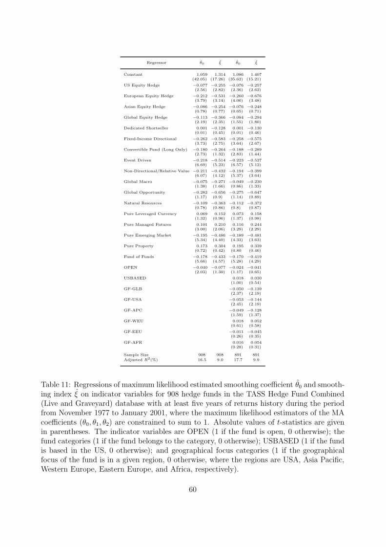
Regressor θ0 ξ θ0 ξ

Constant 1.059 1.314 1.086 1.407(42.05) (17.26) (35.62) (15.21)

US Equity Hedge −0.077 −0.255 −0.076 −0.257(2.56) (2.82) (2.36) (2.62)

European Equity Hedge −0.212 −0.531 −0.260 −0.676(3.79) (3.14) (4.06) (3.48)

Asian Equity Hedge −0.086 −0.254 −0.076 −0.248(0.78) (0.77) (0.65) (0.71)

Global Equity Hedge −0.113 −0.366 −0.084 −0.294(2.19) (2.35) (1.55) (1.80)

Dedicated Shortseller 0.001 −0.128 0.001 −0.130(0.01) (0.45) (0.01) (0.46)

Fixed-Income Directional −0.262 −0.583 −0.258 −0.575(3.73) (2.75) (3.64) (2.67)

Convertible Fund (Long Only) −0.180 −0.264 −0.188 −0.289(2.73) (1.32) (2.83) (1.44)

Event Driven −0.218 −0.514 −0.223 −0.527(6.69) (5.23) (6.57) (5.12)

Non-Directional/Relative Value −0.211 −0.432 −0.194 −0.399(6.07) (4.12) (5.37) (3.64)

Global Macro −0.075 −0.271 −0.049 −0.230(1.38) (1.66) (0.86) (1.33)

Global Opportunity −0.282 −0.656 −0.275 −0.647(1.17) (0.9) (1.14) (0.89)

Natural Resources −0.109 −0.363 −0.112 −0.372(0.78) (0.86) (0.8) (0.87)

Pure Leveraged Currency 0.069 0.152 0.073 0.158(1.32) (0.96) (1.37) (0.98)

Pure Managed Futures 0.101 0.210 0.116 0.244(3.00) (2.06) (3.29) (2.29)

Pure Emerging Market −0.195 −0.486 −0.189 −0.481(5.34) (4.40) (4.33) (3.63)

Pure Property 0.173 0.304 0.195 0.339(0.72) (0.42) (0.80 (0.46)

Fund of Funds −0.178 −0.433 −0.170 −0.419(5.66) (4.57) (5.28) (4.29)

OPEN −0.040 −0.077 −0.024 −0.041(2.03) (1.30) (1.17) (0.65)

USBASED 0.018 0.030(1.00) (0.54)

GF-GLB −0.050 −0.139(2.37) (2.19)

GF-USA −0.053 −0.144(2.45) (2.19)

GF-APC −0.049 −0.128(1.59) (1.37)

GF-WEU 0.018 0.052(0.61) (0.58)

GF-EEU −0.011 −0.045(0.26) (0.35)

GF-AFR 0.016 0.054(0.28) (0.31)

Sample Size 908 908 891 891

Adjusted R2(%) 16.5 9.0 17.7 9.9

Table 11: Regressions of maximum likelihood estimated smoothing coefficient θ0 and smooth-ing index ξ on indicator variables for 908 hedge funds in the TASS Hedge Fund Combined(Live and Graveyard) database with at least five years of returns history during the periodfrom November 1977 to January 2001, where the maximum likelihood estimators of the MAcoefficients (θ0, θ1, θ2) are constrained to sum to 1. Absolute values of t-statistics are givenin parentheses. The indicator variables are OPEN (1 if the fund is open, 0 otherwise); thefund categories (1 if the fund belongs to the category, 0 otherwise); USBASED (1 if the fundis based in the US, 0 otherwise); and geographical focus categories (1 if the geographicalfocus of the fund is in a given region, 0 otherwise, where the regions are USA, Asia Pacific,Western Europe, Eastern Europe, and Africa, respectively).

60

Category N

θ0 θ1 θ2 ξ D.W. R2(%)

Mean SD Mean SD Mean SD Mean SD Mean SD Mean SD

Not Categorized 111 0.659 8.696 0.459 9.363 −0.118 2.260 167.540 1432.164 1.86 0.33 13.6 16.8US Equity Hedge 162 0.695 1.502 0.094 0.415 0.211 1.220 4.427 38.503 1.80 0.28 26.1 17.5European Equity Hedge 22 0.561 0.155 0.340 0.683 0.099 0.708 1.386 4.287 1.76 0.19 18.0 10.8Asian Equity Hedge 5 0.405 0.252 0.323 0.179 0.272 0.088 0.425 0.086 1.82 0.24 7.4 4.5Global Equity Hedge 27 0.846 0.400 0.057 0.331 0.097 0.364 1.115 0.913 1.65 0.22 22.1 19.8Dedicated Shortseller 7 0.908 0.182 0.115 0.101 −0.023 0.203 0.911 0.360 1.94 0.16 43.0 14.7Fixed-Income Directional 13 −1.437 6.398 4.385 14.552 −1.948 8.179 320.099 1151.235 1.62 0.29 13.1 9.9Convertible Fund (Long Only) 15 0.538 0.262 0.343 0.152 0.120 0.178 0.536 0.219 1.53 0.24 25.0 15.0Event Driven 109 0.582 0.479 0.293 0.493 0.125 0.225 0.958 3.568 1.63 0.36 18.0 11.3Non-Directional/Relative Value 85 0.643 4.057 0.895 2.321 −0.538 4.761 45.493 244.844 1.62 0.46 12.2 9.2Global Macro 24 0.558 0.349 0.194 0.341 0.247 0.190 0.674 0.409 1.76 0.28 13.5 8.0Global Opportunity 1 0.619 — 0.191 — 0.191 — 0.455 — 1.55 — 30.9 —Natural Resources 3 0.691 0.138 0.106 0.087 0.203 0.068 0.551 0.163 1.88 0.31 2.6 0.9Pure Leveraged Currency 26 −0.080 1.376 0.360 1.066 0.720 1.987 7.363 24.457 1.89 0.16 4.4 6.0Pure Managed Futures 93 −0.032 1.588 0.696 1.649 0.336 1.611 8.350 26.079 1.99 0.26 5.9 5.9Pure Emerging Market 72 0.899 0.801 0.157 0.465 −0.056 0.452 1.883 6.486 1.51 0.29 22.8 10.6Pure Property 1 1.319 — −0.024 — −0.295 — 1.828 — 2.31 — 15.4 —Fund of Funds 132 0.674 1.516 −0.049 2.566 0.375 3.059 18.694 171.624 1.63 0.30 21.6 15.0All 908 0.554 3.534 0.366 3.950 0.081 2.401 34.268 529.561 1.73 0.34 17.8 15.1

Table 12: Means and standard deviations of linear regression estimates of MA(2) smoothing process Rot = θ0Rt+θ1Rt−1+θ2Rt−2,

ξ ≡ θ20 + θ2

1 + θ22 under the assumption of a linear single-factor model for Rt where the factor is the total return of the S&P

500 Index, for 908 hedge funds in the TASS Hedge Fund Combined (Live and Graveyard) database with at least five years ofreturns history during the period from November 1977 to January 2001.

61

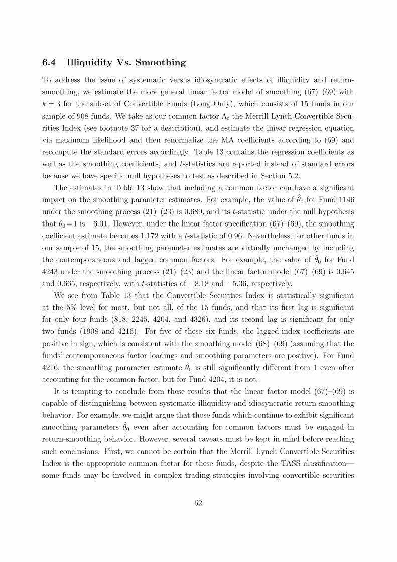
6.4 Illiquidity Vs. Smoothing

To address the issue of systematic versus idiosyncratic effects of illiquidity and return-

smoothing, we estimate the more general linear factor model of smoothing (67)–(69) with

k = 3 for the subset of Convertible Funds (Long Only), which consists of 15 funds in our

sample of 908 funds. We take as our common factor Λt the Merrill Lynch Convertible Secu-

rities Index (see footnote 37 for a description), and estimate the linear regression equation

via maximum likelihood and then renormalize the MA coefficients according to (69) and

recompute the standard errors accordingly. Table 13 contains the regression coefficients as

well as the smoothing coefficients, and t-statistics are reported instead of standard errors

because we have specific null hypotheses to test as described in Section 5.2.

The estimates in Table 13 show that including a common factor can have a significant

impact on the smoothing parameter estimates. For example, the value of θ0 for Fund 1146

under the smoothing process (21)–(23) is 0.689, and its t-statistic under the null hypothesis

that θ0 =1 is −6.01. However, under the linear factor specification (67)–(69), the smoothing

coefficient estimate becomes 1.172 with a t-statistic of 0.96. Nevertheless, for other funds in

our sample of 15, the smoothing parameter estimates are virtually unchanged by including

the contemporaneous and lagged common factors. For example, the value of θ0 for Fund

4243 under the smoothing process (21)–(23) and the linear factor model (67)–(69) is 0.645

and 0.665, respectively, with t-statistics of −8.18 and −5.36, respectively.

We see from Table 13 that the Convertible Securities Index is statistically significant

at the 5% level for most, but not all, of the 15 funds, and that its first lag is significant

for only four funds (818, 2245, 4204, and 4326), and its second lag is significant for only

two funds (1908 and 4216). For five of these six funds, the lagged-index coefficients are

positive in sign, which is consistent with the smoothing model (68)–(69) (assuming that the

funds’ contemporaneous factor loadings and smoothing parameters are positive). For Fund

4216, the smoothing parameter estimate θ0 is still significantly different from 1 even after

accounting for the common factor, but for Fund 4204, it is not.

It is tempting to conclude from these results that the linear factor model (67)–(69) is

capable of distinguishing between systematic illiquidity and idiosyncratic return-smoothing

behavior. For example, we might argue that those funds which continue to exhibit significant

smoothing parameters θ0 even after accounting for common factors must be engaged in

return-smoothing behavior. However, several caveats must be kept in mind before reaching

such conclusions. First, we cannot be certain that the Merrill Lynch Convertible Securities

Index is the appropriate common factor for these funds, despite the TASS classification—

some funds may be involved in complex trading strategies involving convertible securities

62

while others are engaged in simpler buy-and-hold strategies.44 Regressing a fund’s returns

on a highly serially correlated common factor that is not directly relevant to that fund’s

investment process will, nevertheless, have an effect on the smoothing-parameter estimates

θk, and the effect may be in either direction depending on the relation between the common

factor and the fund’s observed returns. Second, even if a common factor can account for

much of the serial correlation in a fund’s observed returns, an explanation for the source of

the factor’s serial correlation is still required—if the fund is a buy-and-hold version of the

common factor, e.g., a fund-of-funds designed to replicate the CSFB/Tremont Convertible

Arbitrage Index, then it is of small comfort to investors in such a fund-of-funds that there

is not much smoothing in observed returns beyond what is already present in the common

factor. And finally, no econometric model can fully capture the many qualitative and often

subjective characteristics of a fund’s investment process, and such information is likely to

be of particular relevance in distinguishing between illiquidity and smoothed returns at the

fund level.

These caveats suggest that a more comprehensive econometric analysis of hedge-fund

returns may be worthwhile, with particular emphasis on constructing common factors for

hedge funds with similar investment mandates and processes. By developing a better under-

standing for the common risk exposures that certain hedge funds share, it may be possible

to differentiate between systematic and idiosyncratic illiquidity and provide investors and

managers with a more refined set of tools with which to optimize their investment plans.

6.5 Smoothing-Adjusted Sharpe Ratio Estimates

For each of the 908 funds in our sample, we compute annual Sharpe ratios in three ways

relative to a benchmark return of 0: the standard method (√

12 times the ratio of the mean

monthly return to the monthly return standard deviation), the serial-correlation-adjusted

method in Lo (2002), and the small-sample method described in Section 5.4. The results are

summarized in Table 14.

The largest differences between standard and smoothing-adjusted Sharpe ratios are found

in the same categories that the smoothing-process estimates of Section 6.2 identified as

the most illiquid: Fixed-Income Directional (20.3% higher average Sharpe ratio relative

to SR∗∗), Convertible Fund (Long Only) (17.8%), Non-Directional/Relative Value (16.0%),

44 In particular, of the 15 “Convertible Fund (Long Only)” funds in our sample, 12 funds involve long-only positions in convertible bonds, possibly with a limited degree of leverage, but with no equity or creditprotection, and the remaining 3 funds (4204, 4145 and 4326) are convertible arbitrage funds that involvelong positions in convertible bonds and short positions in the corresponding stocks. We thank Stephen Juppof TASS for providing us with this information.

63

Code T Periodµ γ0 γ1 γ2 Maximum Likelihood Smoothing Parameter Estimates

(t-stat) (t-stat) (t-stat) (t-stat) θ0 t(θ0) θ1 t(θ1) θ2 t(θ2) ξ

31 90 199307–200012 −1.159 1.171 0.036 −0.110 0.903 −0.55 −0.296 −2.39 0.393 6.42 1.06(−2.28) (11.51) (0.36) (−0.92) 0.794 −3.24 0.083 1.27 0.123 1.94 0.65

818 72 199502–200101 −0.754 0.387 0.168 0.014 0.986 −0.10 0.139 1.31 −0.124 −0.96 1.01(−1.66) (5.84) (1.98) (0.15) 0.759 −3.46 0.261 4.71 −0.019 −0.28 0.64

843 79 199407–200101 −0.716 0.340 0.144 0.106 0.971 −0.18 0.094 0.93 −0.065 −0.51 0.96(−1.86) (4.50) (1.61) (0.97) 0.847 −2.02 0.159 2.34 −0.006 −0.08 0.74

1146 94 199010–199807 −1.503 1.043 0.138 −0.029 1.172 0.96 −0.044 −0.30 −0.128 −0.98 1.39(−7.59) (13.15) (1.75) (−0.39) 0.689 −6.01 0.187 3.79 0.124 2.40 0.53

1148 73 199501–200101 −0.966 0.617 0.106 −0.009 1.125 0.51 0.312 3.16 −0.437 −1.72 1.55(−3.07) (10.49) (1.25) (−0.11) 0.795 −2.81 0.211 3.39 −0.006 −0.08 0.68

1908 81 199405–200101 −1.191 1.325 0.121 −0.425 0.989 −0.06 0.052 0.42 −0.041 −0.37 0.98(−1.37) (10.51) (0.82) (−2.09) 0.909 −1.12 0.140 1.93 −0.049 −0.60 0.85

2245 67 199507–200101 −0.607 0.287 0.174 0.034 0.938 −0.36 0.087 0.70 −0.025 −0.22 0.89(−1.27) (3.48) (2.37) (0.31) 0.870 −1.53 0.173 2.34 −0.043 −0.50 0.79

2564 63 199511–200101 −0.621 0.291 0.108 0.123 0.866 −0.67 0.279 2.17 −0.145 −0.90 0.85(−1.10) (3.22) (1.39) (1.36) 0.778 −2.86 0.303 5.45 −0.080 −1.03 0.70

3099 73 199501–200101 0.093 −0.040 −0.047 0.018 0.632 −4.10 0.104 1.71 0.264 5.49 0.48(0.41) (−0.96) (−1.32) (0.39) 0.615 −8.31 0.121 2.37 0.263 5.68 0.46

4145 63 199511–200101 −0.487 0.368 −0.094 −0.031 2.042 4.82 0.015 0.03 −1.058 −1.08 5.29(−0.73) (2.14) (−0.61) (−0.14) 2.077 4.41 0.161 1.16 −1.238 −5.07 5.87

4204 72 199501–200012 −0.876 0.303 0.304 0.069 0.769 −1.26 0.122 0.85 0.109 1.46 0.62(−2.88) (4.52) (6.37) (0.95) 0.678 −5.53 0.217 4.08 0.105 1.80 0.52

4216 104 199206–200101 −0.115 0.012 0.012 0.079 0.650 −4.60 0.151 3.47 0.200 4.60 0.48(−0.61) (0.56) (0.50) (2.09) 0.663 −7.48 0.134 2.84 0.202 4.49 0.50

4243 118 199101–200010 −0.322 0.036 0.110 0.081 0.665 −5.36 0.270 6.24 0.066 0.89 0.52(−1.07) (0.59) (1.70) (1.15) 0.645 −8.18 0.279 7.76 0.076 1.76 0.50

4295 82 199403–200012 −0.014 0.039 −0.032 0.014 0.894 −0.61 −0.031 −0.22 0.136 1.63 0.82(−0.07) (0.51) (−0.72) (0.21) 0.893 −1.37 0.009 0.10 0.098 1.26 0.81

4326 149 198807–200101 −0.154 0.082 0.039 0.021 0.700 −4.71 0.229 6.40 0.071 1.40 0.55(−2.10) (6.02) (2.60) (1.24) 0.662 −8.62 0.243 7.02 0.095 2.43 0.51

Table 13: Maximum likelihood estimates of linear regression model with MA(2) errors, Rot = µ + γ0Λt + γ1Λt−1 + γ2Λt−2 + ut,

ut = θ0εt + θ1εt−1 + θ2εt−2, subject to the normalization 1 = θ0 + θ1 + θ2, for all 15 Convertible Funds (Long Only) amongthe sample of 908 hedge funds in the TASS Hedge Fund Combined (Live and Graveyard) database with at least five yearsof returns history during the period from November 1977 to January 2001. The factor Λt is taken to be the Merrill LynchConvertible Securities Index. For comparison, maximum likelihood estimates of θ0, θ1, θ2, and t-statistics from the MA(2)smoothing process Ro

t = θ0Rt + θ1Rt−1 + θ2Rt−2, subject to the normalization 1 = θ0 + θ1 + θ2, are provided below each of themain rows. t-statistics are computed with respect to the null hypothesis that the coefficient is 0, except for θ0, for which thenull hypothesis θ0 = 1 is used, hence the t-statistic is computed as (θ0 − 1)/SE(θ0).

64

Pure Emerging Market (16.3%), and Fund of Funds (17.8%). For two categories—Dedicated

Shortseller and Managed Futures—the bias is reversed, a result of negative serial correlation

in their returns. For the other categories, Table 14 shows that the smoothing-adjusted Sharpe

ratios are similar in magnitude to the usual estimates. These differences across categories

suggest the importance of taking illiquidity and smoothed returns into account in evaluating

the performance of hedge funds.

Category

Sharpe Ratios For Combined Sample

NSR SR∗ SR∗∗

Mean SD Mean SD Mean SD

Not Categorized 111 1.12 1.09 1.06 0.87 1.00 0.82US Equity Hedge 162 1.26 0.75 1.31 0.75 1.23 0.69European Equity Hedge 22 1.43 0.74 1.43 0.80 1.33 0.74Asian Equity Hedge 5 0.50 0.39 0.52 0.39 0.49 0.37Global Equity Hedge 27 0.90 0.61 0.95 0.66 0.89 0.61Dedicated Shortseller 7 0.28 0.59 0.32 0.64 0.30 0.61Fixed-Income Directional 13 2.02 2.35 1.80 2.23 1.68 2.06Convertible Fund (Long Only) 15 1.83 1.20 1.66 0.85 1.55 0.80Event Driven 109 2.36 1.45 2.21 1.57 2.08 1.47Non-Directional/Relative Value 85 2.20 1.86 2.03 2.39 1.89 2.22Global Macro 24 1.08 0.67 1.14 0.73 1.07 0.70Global Opportunity 1 −0.56 — −0.39 — −0.37 —Natural Resources 3 0.60 0.25 0.56 0.23 0.52 0.21Pure Leveraged Currency 26 0.63 0.49 0.65 0.50 0.61 0.47Pure Managed Futures 93 0.54 0.55 0.63 0.60 0.60 0.56Pure Emerging Market 72 0.39 0.45 0.36 0.44 0.34 0.40Pure Property 1 0.42 — 0.45 — 0.41 —Fund of Funds 132 1.44 1.01 1.30 0.88 1.22 0.82

All 908 1.32 1.24 1.27 1.27 1.19 1.18

Table 14: Means and standard deviations of Sharpe ratios of 908 hedge funds in the TASSHedge Fund Combined (Live and Graveyard) database with at least five years of returnshistory during the period from November 1977 to January 2001. SR is the standard Sharperatio, SR∗ is the smoothing-adjusted Sharpe ratio of Lo (2002), and SR∗∗ is the smoothing-adjusted Sharpe ratio using σNW. All Sharpe ratios are computed with respect to a 0benchmark.

65

7 Conclusions

Although there are several potential explanations for serial correlation in asset returns, we

have argued in this paper that the serial correlation present in the returns of hedge funds

is due primarily to illiquidity and smoothed returns. Using a simple econometric model

in which observed returns are a finite moving-average of unobserved economic returns, we

are able to generate empirically realistic levels of serial correlation for historical hedge-fund

returns while, at the same time, explaining the findings of Asness, Krail and Liew (2001)

regarding the significance of lagged market returns in market-model regressions for hedge

funds. Although our moving-average specification is similar to some of the early models of

nonsynchronous trading, our motivation is quite different and is meant to cover a broader

set of factors that give rise to serial correlation and smoothed returns, even in the presence

of synchronously recorded prices.

Maximum likelihood estimates of our smoothing model for the returns of 908 hedge funds

in the TASS Hedge Fund database yield empirically plausible estimates of smoothing coeffi-

cients and suggest that simple time-series measures such as our smoothing index may serve

as useful proxies for a hedge fund’s illiquidity risk exposure. In some cases, our econometric

model may also be useful for flagging possible cases of deliberate performance-smoothing

behavior, although additional information will need to be gathered before any firm conclu-

sions regarding such behavior can be made. Regardless of the sources of serial correlation,

illiquidity exposure is the main implication and this has potentially important consequences

for both managers and investors. Therefore, we also develop a set of tools for quantifying the

degree of smoothing in the data and adjusting for smoothed returns in computing perfor-

mance statistics such as means, variances, market betas, and Sharpe ratios, and derive their

asymptotic distributions using continuous-record asymptotics that can better accommodate

the small sample sizes of most hedge-fund datasets.

Our empirical results suggest several applications for our econometric model of illiquidity

and smoothed returns. Despite the general consistency of our empirical results with common

intuition regarding the levels of illiquidity among the various hedge-fund investment styles,

the variation in estimated smoothing coefficients within each category indicates that there

may be better ways of categorizing hedge funds. Given the importance of liquidity for the

typical hedge-fund investor, it may be useful to subdivide each style category into “liquidity

tranches” defined by our smoothing index. This may prove to be especially useful in iden-

tifying and avoiding the potential wealth transfers between new and existing investors that

can occur from the opportunistic timing of hedge-fund investments and redemptions. Alter-

natively, our smoothing parameter estimates may be used to compute illiquidity exposure

66

measures for portfolios of hedge funds or fund of funds, which may serve as the basis for a

more systematic approach to managing portfolios that include alternative investments.

Although we have focused on hedge funds in this paper, our analysis may be applied

to other investments and asset classes, e.g., real estate, venture capital, private equity, art

and other collectibles, and other assets for which illiquidity and smoothed returns are even

more problematic, and where the estimation of smoothing profiles can be particularly useful

for providing investors with risk transparency. More generally, our econometric model may

be applied to a number of other contexts in which there may be a gap between reported

results and economic realities. For example, recent events surrounding the collapse of Enron

and other cases of corporate accounting irregularities have created renewed concerns about

“earnings management” in which certain corporations are alleged to have abused accounting

conventions so as to smooth earnings, presumably to give the appearance of stability and

consistent growth.45 The impact of such smoothing can sometimes be “undone” using an

econometric model such as ours.

There are a number of outstanding issues regarding our analysis of illiquidity and smoothed

returns that warrant further study. Perhaps the most pressing issue is whether the proximate

source of smoothing is inadvertent or deliberate. Our linear regression model with contem-

poraneous and lagged common factors may serve as the starting point for distinguishing

between systematic illiquidity versus idiosyncratic smoothing behavior. However, this issue

is likely to require additional information about each fund along the lines of Chandar and

Bricker’s (2002) study, e.g., the size of the fund, the types of the securities in which the fund

invests, the accounting conventions used to mark the portfolio, the organization’s compen-

sation structure, and other operational aspects of the fund. With these additional pieces

of information, we may construct more relevant common factors for our linear-regression

framework, or relate the cross-sectional variation in smoothing coefficients to assets under

management, security type, fee structure, and other characteristics, yielding a more complete

picture of the sources of smoothed returns.

It may also be fruitful to view the hedge-fund industry from a broader perspective, one

that acknowledges the inherent capacity constraints of certain types of strategies as well

as the time lags involved in shifting assets from one type to another. Because of the in-

evitable cross-sectional differences in the performance of hedge-fund styles, assets often flow

in loosely coordinated fashion from one style to another, albeit under various institutional

restrictions such as calendar-specific periods of liquidity, tiered redemption schedules, re-

demption fees, and other frictions. The interactions between asset flows and institutional

45See Beneish (2001) and Healy and Wahlen (1999) for reviews of the extensive literature on earningsmanagement.

67

rigidities—especially over time—may sometimes cause statistical side-effects that include

periodicities in performance and volatility, time-varying correlations, structural breaks, and

under certain conditions, serial correlation. The dynamics of the hedge-fund industry are

likely to be quite different than that of more traditional investment products, hence the

“ecological” framework of Niederhoffer (1998, Chapter 15), Farmer (1998), and Farmer and

Lo (1999), or the system dynamics approach of Getmansky and Lo (2003) might be more

conducive paradigms for addressing these issues.

Finally, from the hedge-fund investor’s perspective, a natural extension of our analysis

is to model illiquidity directly and quantify the illiquidity premium associated with each

hedge-fund investment style, perhaps in a linear-factor framework such as Chordia, Roll

and Subrahmanyam (2000) and Pastor and Stambaugh (2002). Whether such factor models

can forecast liquidity crises like August 1998, and whether there are “systematic” illiquidity

factors that are common to categories of hedge funds are open questions that are particularly

important in the context of hedge-fund investments. We plan to address these and other

related questions in our ongoing research.

68

A Appendix

Proofs of Propositions 3, 4, and 5 are provided in Sections A.1, A.2, and A.3, respectively.

Section A.4 provides definitions of the 17 categories from TASS, and Section A.5 contains

additional empirical results.

A.1 Proof of Proposition 3

The constraint (49) may be used to substitute out θ0, hence we need only consider (θ1, θ2).

Now it is well known that in the standard MA(2) specification where the usual identification

condition is used in place of (49), i.e.,

Xt = εt + aεt−1 + bεt−2 ,

the asymptotic distribution of the maximum likelihood estimators (a, b) is given by:

√T

([a

b

]−[

a

b

])a∼ N (0,V) (A.1)

where

V ≡[

1 − b2 a(1 − b)

a(1 − b) 1 − b2

]. (A.2)

But under our normalization (49), there is a simple functional relation between (a, b) and

(θ1, θ2):

θ1 =a

1 + a + b, θ2 =

b

1 + a + b. (A.3)

Therefore, we can apply the delta method to obtain the asymptotic distribution of (θ1, θ2)

as:

√T

([θ1

θ2

]−[

θ1

θ2

])a∼ N (0,JVJ′) (A.4)

69

where the matrix J is Jacobian associated with (A.3):

J =1

(1 + a + b)2

[1 + b −a

−b 1 + a

]. (A.5)

Then we have:

JVJ′ =

1

(1 + a + b)3

[−(1 + b)(−1 + a − ab + b2) b(−1 + a − ab + b2)

b(−1 + a − ab + b2) −(−1 + b)(−1 + a − ab + b2)

](A.6)

and solving for a and b as a function of θ1 and θ2 using (A.3) and substituting these expres-

sions into A.6 yields the desired result.

The process Xt is invertible if and only if the roots of characteristic polynomial

f(x) = θ0x2 + θ1x + θ2 (A.7)

lie inside the unit circle in the complex plane. It is easy to see that this is equivalent to the

condition that the roots of

f(x) = f

(z + 1

z − 1

)=

z2 + 2(1 − θ1 − 2θ2)z + 1 − 2θ1

(z − 1)2(A.8)

lie in the left half-plane (Samuelson, 1941, was perhaps the first to state this result). Apply-

ing the Routh-Hurwitz necessary and sufficient conditions to (A.8) then yields the desired

result.

A.2 Proof of Proposition 4

Theorem 1 [Herrndorf (1984)] If {εt} satisfies the following assumptions:

(A1) E[εt] = µ for all t.

(A2) supt E[|εt−µ|β] < ∞ for some β > 2 .

(A3) 0 < σ2o = limT→∞ E

[1T

(∑nj=1(εj−µ

)2]

< ∞ .

70

(A4) {εt} is strong-mixing with mixing coefficients αk that satisfy:

∞∑

j=1

α1− 2

β

j < ∞ . (A.9)

then as n increases without bound,

Wn(s) ≡ 1

σo

√n

[ns]∑

j=1

(εj−µ) ⇒ W (s) , s ∈ [0, 1] (A.10)

where [ns] denotes the greater integer less than or equal to ns and ‘⇒’ denotes weak conver-

gence.

With these results in hand, we are ready to prove Proposition 4. Let returns Rt be given by:

Rt = εt (A.11)

where εt satisfies assumptions (A1)–(A4) of Theorem 1, and recall:

µ =1

T

T∑

1

εt (A.12)

σ2NW =

1

T

T∑

1

(εt − µ)2 +2

T

θ∑

j=1

(1 − j

θ + 1)

T∑

t=j+1

(εt − µ)(εt−j − µ) (A.13)

= I1 + I2 where (A.14)

I1 ≡ 1

T

T∑

1

(εt − µ)2 (A.15)

I2 ≡ 2

T

θ∑

j=1

(1 − j

θ + 1)

T∑

t=j+1

(εt − µ)(εt−j − µ) (A.16)

Observe that

I1 =1

T

T∑

1

(εt − µ)2 =1

T

T∑

1

ε2t − µ2 p→ σ2

ε (A.17)

71

where

σ2ε ≡ lim

t→∞

1

T

T∑

1

ε2t = E[ε2

t ] . (A.18)

Now the second term I2 can be written as:

I2T (m + 1)

2=

m∑

j=0

(m + 1 − j)T∑

t=j+1

(εt − µ)(εt−j − µ) = J1 + J2 + J3 (A.19)

where

J1 ≡m∑

j=0

(m+1− j)

T∑

t=j+1

εtεt−j (A.20)

J2 ≡m∑

j=0

(m+1−j)

T∑

t=j+1

µ(εt + εt−j) (A.21)

J3 ≡m∑

j=0

(m+1−j)T∑

t=j+1

µ2 (A.22)

72

Consider the first term in (A.19):

J1 =

m∑

j=0

(m + 1 − j)

T∑

t=j+1

εtεt−j = m(ε1ε2 + ε2ε3 + · · · + εT−1εT ) +

(m − 1)(ε1ε3 + ε2ε4 + · · ·+ εT−2εT ) +

(ε1εm+1 + ε2εm+2 + · · · + εT−mεT ) (A.23)

= ε1

((S2 − S1) + (S3 − S1) + · · ·+ (Sm+1 − S1)

)+ · · · +

εT−m

((ST−m+1 − ST−m) + · · · + (ST − ST−m)

)+

εT−m+1

((ST−m+2 − ST−m+1) + · · ·+ 2(ST − ST−m+1)

)+ · · · +

εT−1

(m(ST − ST−1)

)(A.24)

= ε1(S2 + S3 + · · ·+ Sm+1) − mε1S1 + · · · +

εT−m(ST−m+1 + · · ·+ ST ) − mεT−mST−m +

εT−m+1(ST−m+2 + · · ·+ 2ST ) − mεT−m+1ST−m+1 + · · · +

εT−1mST − mεT−1ST−1 (A.25)

= S2S1 + S3S2 + · · · + Sm+1Sm + Sm+2(Sm+1 − S1) + · · · +

ST (ST−1 − ST−m−1) + ST (εT−m+1 + · · ·+ mεT−1) − mT−1∑

t=1

εtSt (A.26)

=

T−1∑

t=1

S2t − (m − 1)

T−1∑

t=1

εtSt −T−(m+1)∑

t=1

StSt+m+1 +

ST

(mST−1 −

T−1∑

t=T−m

St

)(A.27)

When the Functional Central Limit Theorem is applied to (A.27), we have:

J1/T2 ⇒ σ2

(∫ 1

0

W (r)(W (r) − W (min(r + λ, 1)))dr

)−

(m − 1)

2T(σ2W 2(1) + σ2

ε ) +m

Tσ2W 2(1) (A.28)

73

Now the second term in (A.19) can be rewritten as:

J2 = −m∑

j=1

(m + 1 − j)

T∑

t=j+1

µ(εt + εt−j) (A.29)

= −µm∑

j=1

(m + 1 − j)(ST − Sj + ST−j) (A.30)

= − m(m + 1)

2µST − µ

m∑

j=1

(m + 1 − j)(ST−j − Sj) (A.31)

and applying the Functional Central Limit Theorem to (A.31) yields

J2/T2 ⇒ − m(m + 1)

2T 2σ2W 2(1) − σ2W (1)

∫ λ

0

(λ− r)(W (1− r)−W (r))dr . (A.32)

The third term of (A.19) can be rewritten in a similar manner:

J3 =m∑

j=1

(m + 1 − j)T∑

t=j+1

µ2 = µ2m∑

j=1

(m + 1 − j)(T − j − 1) (A.33)

= µ2

m∑

j=1

(j2 − j(T + m) + (m + 1)(T − 1)) (A.34)

= µ2m(m + 1)(3T − m − 5)

6(A.35)

and applying the Functional Central Limit Theorem to (A.35) yields:

J3/T2 ⇒ σ2W 2(1)

(1 + m)m(3T − m − 5)

6T 3. (A.36)

Combining (A.28), (A.32) and (A.36) shows that:

I2 ⇒ 2

λσ2

(∫ 1

0

W (r)[W (r) − W (min(r + λ, 1))

]dr −

W (1)

∫ λ

0

(λ − r)(W (1 − r) − W (r))dr

)+ σ2W 2(1)(1 − λ2

3) − σ2

ε (A.37)

74

and summing (A.17) and (A.37) yields the desired result.

A.3 Proof of Proposition 5

Given the weak convergence of σ2

NW to the functional f(W ) in (87), Proposition 5 is an

almost trivial consequence of the following well-known result:

Theorem 2 [Extended Continuous Mapping Theorem]46 Let hn and h be measurable map-

pings from D[0, 1]—the space of all functions on [0, 1] that are right continuous with left-hand

limits—to itself and denote by E the set of x ∈ D[0, 1] such that hn(xn) → h(x) fails to hold

for some sequence xn converging to x. If Wn(s) ⇒ W (s) and E is of Wiener-measure

zero, i.e. P(W ∈ E) = 0, then hn(Wn) ⇒ h(W ).

A.4 TASS Fund Category Definitions

The following is a list of category descriptions, taken directly from TASS documentation,

that define the criteria used by TASS in assigning funds in their database to one of 17

possible categories:

Equity Hedge This directional strategy involves equity-oriented investing on both the long and short sidesof the market. The objective is not to be market neutral. Managers have the ability to shift fromvalue to growth, from small to medium to large capitalization stocks, and from a net long positionto a net short position. Managers may use futures and options to hedge. The focus may be regional,such as long/short US or European equity, or sector specific, such as long and short technology orhealthcare stocks. Long/short equity funds tend to build and hold portfolios that are substantiallymore concentrated than those of traditional stock funds. US equity Hedge, European equity Hedge,Asian equity Hedge and Global equity Hedge is the regional Focus.

Dedicated Short Seller Short biased managers take short positions in mostly equities and derivatives.The short bias of a manager’s portfolio must be constantly greater than zero to be classified in thiscategory.

Fixed Income Directional This directional strategy involves investing in Fixed Income markets only ona directional basis.

Convertible Arbitrage This strategy is identified by hedge investing in the convertible securities of acompany. A typical investment is to be long the convertible bond and short the common stock of thesame company. Positions are designed to generate profits from the fixed income security as well asthe short sale of stock, while protecting principal from market moves.47

46See Billingsley (1968) for a proof.47Note that the category closest to this definition in the TASS database is “Convertible Fund (Long

Only)”, which is related to but different from convertible arbitrage—see footnote 44 for details. TASSrecently changed their style classifications, and now defines “Convertible Arbitrage” as a distinct category.

75

Event Driven This strategy is defined as ‘special situations’ investing designed to capture price movementgenerated by a significant pending corporate event such as a merger, corporate restructuring, liquida-tion, bankruptcy or reorganization. There are three popular sub-categories in event-driven strategies:risk (merger) arbitrage, distressed/high yield securities, and Regulation D.

Non Directional/Relative Value This investment strategy is designed to exploit equity and/or fixedincome market inefficiencies and usually involves being simultaneously long and short matched marketportfolios of the same size within a country. Market neutral portfolios are designed to be either betaor currency neutral, or both.

Global Macro Global macro managers carry long and short positions in any of the world’s major capitalor derivative markets. These positions reflect their views on overall market direction as influencedby major economic trends and or events. The portfolios of these funds can include stocks, bonds,currencies, and commodities in the form of cash or derivatives instruments. Most funds invest globallyin both developed and emerging markets.

Global Opportunity Global macro managers carry long and short positions in any of the world’s majorcapital or derivative markets on an opportunistic basis. These positions reflect their views on overallmarket direction as influenced by major economic trends and or events. The portfolios of these fundscan include stocks, bonds, currencies, and commodities in the form of cash or derivatives instruments.Most funds invest globally in both developed and emerging markets.

Natural Resources This trading strategy has a focus for the natural resources around the world.

Leveraged Currency This strategy invests in currency markets around the world.

Managed Futures This strategy invests in listed financial and commodity futures markets and currencymarkets around the world. The managers are usually referred to as Commodity Trading Advisors, orCTAs. Trading disciplines are generally systematic or discretionary. Systematic traders tend to useprice and market specific information (often technical) to make trading decisions, while discretionarymanagers use a judgmental approach.

Emerging Markets This strategy involves equity or fixed income investing in emerging markets aroundthe world.

Property The main focus of the investments are property.

Fund of Funds A ‘Multi Manager’ fund will employ the services of two or more trading advisors or HedgeFunds who will be allocated cash by the Trading Manager to trade on behalf of the fund.

A.5 Supplementary Empirical Results

In Tables A.1–A.7, we provide corresponding empirical results to Tables 7–14 but with Live

and Graveyard funds separated so that the effects of survivorship bias can be seen. Of

course, since we still apply our five-year minimum returns history filter to both groups, there

is still some remaining survivorship bias. Tables A.1 and A.2 contain summary statistics for

the two groups of funds, Tables A.3 and A.4 report summary statistics for the maximum

likelihood estimates of the smoothing model (21)–(23), Tables A.5 and A.6 report similar

statistics for the regression model estimates (62) of the smoothing model, and Table A.7

contains smoothing-adjusted Sharpe ratios for the two groups of funds. Finally, Table A.8

76

corresponds to the regressions of Table 11 but with dependent variables θ0 and ξ estimated

by maximum likelihood under the alternate constraint (75).

77

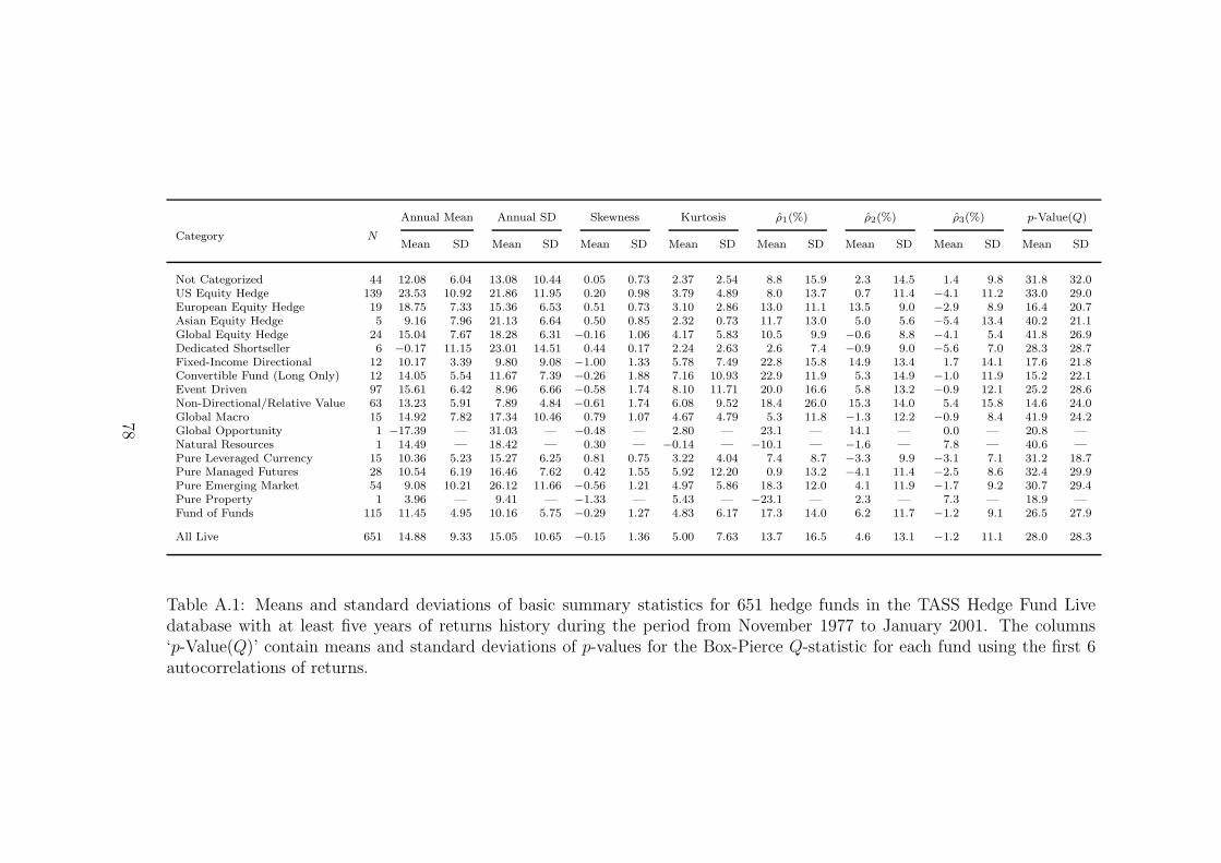
Category N

Annual Mean Annual SD Skewness Kurtosis ρ1(%) ρ2(%) ρ3(%) p-Value(Q)

Mean SD Mean SD Mean SD Mean SD Mean SD Mean SD Mean SD Mean SD

Not Categorized 44 12.08 6.04 13.08 10.44 0.05 0.73 2.37 2.54 8.8 15.9 2.3 14.5 1.4 9.8 31.8 32.0US Equity Hedge 139 23.53 10.92 21.86 11.95 0.20 0.98 3.79 4.89 8.0 13.7 0.7 11.4 −4.1 11.2 33.0 29.0European Equity Hedge 19 18.75 7.33 15.36 6.53 0.51 0.73 3.10 2.86 13.0 11.1 13.5 9.0 −2.9 8.9 16.4 20.7Asian Equity Hedge 5 9.16 7.96 21.13 6.64 0.50 0.85 2.32 0.73 11.7 13.0 5.0 5.6 −5.4 13.4 40.2 21.1Global Equity Hedge 24 15.04 7.67 18.28 6.31 −0.16 1.06 4.17 5.83 10.5 9.9 −0.6 8.8 −4.1 5.4 41.8 26.9Dedicated Shortseller 6 −0.17 11.15 23.01 14.51 0.44 0.17 2.24 2.63 2.6 7.4 −0.9 9.0 −5.6 7.0 28.3 28.7Fixed-Income Directional 12 10.17 3.39 9.80 9.08 −1.00 1.33 5.78 7.49 22.8 15.8 14.9 13.4 1.7 14.1 17.6 21.8Convertible Fund (Long Only) 12 14.05 5.54 11.67 7.39 −0.26 1.88 7.16 10.93 22.9 11.9 5.3 14.9 −1.0 11.9 15.2 22.1Event Driven 97 15.61 6.42 8.96 6.66 −0.58 1.74 8.10 11.71 20.0 16.6 5.8 13.2 −0.9 12.1 25.2 28.6Non-Directional/Relative Value 63 13.23 5.91 7.89 4.84 −0.61 1.74 6.08 9.52 18.4 26.0 15.3 14.0 5.4 15.8 14.6 24.0Global Macro 15 14.92 7.82 17.34 10.46 0.79 1.07 4.67 4.79 5.3 11.8 −1.3 12.2 −0.9 8.4 41.9 24.2Global Opportunity 1 −17.39 — 31.03 — −0.48 — 2.80 — 23.1 — 14.1 — 0.0 — 20.8 —Natural Resources 1 14.49 — 18.42 — 0.30 — −0.14 — −10.1 — −1.6 — 7.8 — 40.6 —Pure Leveraged Currency 15 10.36 5.23 15.27 6.25 0.81 0.75 3.22 4.04 7.4 8.7 −3.3 9.9 −3.1 7.1 31.2 18.7Pure Managed Futures 28 10.54 6.19 16.46 7.62 0.42 1.55 5.92 12.20 0.9 13.2 −4.1 11.4 −2.5 8.6 32.4 29.9Pure Emerging Market 54 9.08 10.21 26.12 11.66 −0.56 1.21 4.97 5.86 18.3 12.0 4.1 11.9 −1.7 9.2 30.7 29.4Pure Property 1 3.96 — 9.41 — −1.33 — 5.43 — −23.1 — 2.3 — 7.3 — 18.9 —Fund of Funds 115 11.45 4.95 10.16 5.75 −0.29 1.27 4.83 6.17 17.3 14.0 6.2 11.7 −1.2 9.1 26.5 27.9

All Live 651 14.88 9.33 15.05 10.65 −0.15 1.36 5.00 7.63 13.7 16.5 4.6 13.1 −1.2 11.1 28.0 28.3

Table A.1: Means and standard deviations of basic summary statistics for 651 hedge funds in the TASS Hedge Fund Livedatabase with at least five years of returns history during the period from November 1977 to January 2001. The columns‘p-Value(Q)’ contain means and standard deviations of p-values for the Box-Pierce Q-statistic for each fund using the first 6autocorrelations of returns.

78

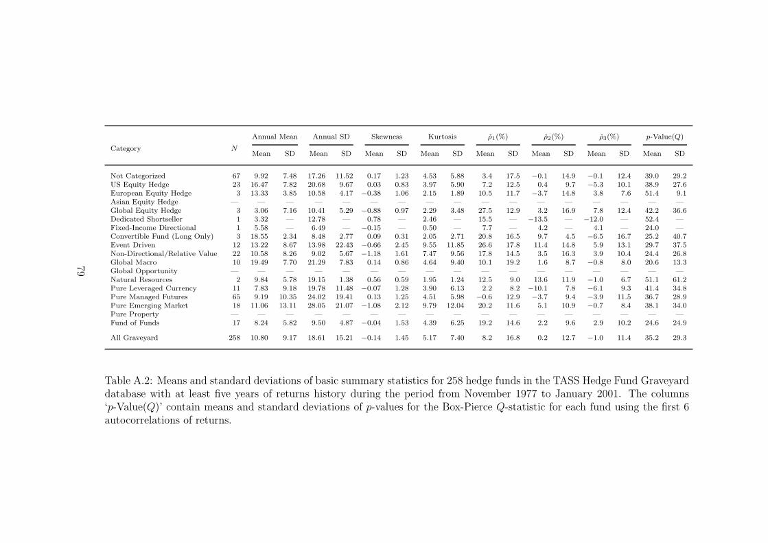
Category N

Annual Mean Annual SD Skewness Kurtosis ρ1(%) ρ2(%) ρ3(%) p-Value(Q)

Mean SD Mean SD Mean SD Mean SD Mean SD Mean SD Mean SD Mean SD

Not Categorized 67 9.92 7.48 17.26 11.52 0.17 1.23 4.53 5.88 3.4 17.5 −0.1 14.9 −0.1 12.4 39.0 29.2US Equity Hedge 23 16.47 7.82 20.68 9.67 0.03 0.83 3.97 5.90 7.2 12.5 0.4 9.7 −5.3 10.1 38.9 27.6European Equity Hedge 3 13.33 3.85 10.58 4.17 −0.38 1.06 2.15 1.89 10.5 11.7 −3.7 14.8 3.8 7.6 51.4 9.1Asian Equity Hedge — — — — — — — — — — — — — — — — —Global Equity Hedge 3 3.06 7.16 10.41 5.29 −0.88 0.97 2.29 3.48 27.5 12.9 3.2 16.9 7.8 12.4 42.2 36.6Dedicated Shortseller 1 3.32 — 12.78 — 0.78 — 2.46 — 15.5 — −13.5 — −12.0 — 52.4 —Fixed-Income Directional 1 5.58 — 6.49 — −0.15 — 0.50 — 7.7 — 4.2 — 4.1 — 24.0 —Convertible Fund (Long Only) 3 18.55 2.34 8.48 2.77 0.09 0.31 2.05 2.71 20.8 16.5 9.7 4.5 −6.5 16.7 25.2 40.7Event Driven 12 13.22 8.67 13.98 22.43 −0.66 2.45 9.55 11.85 26.6 17.8 11.4 14.8 5.9 13.1 29.7 37.5Non-Directional/Relative Value 22 10.58 8.26 9.02 5.67 −1.18 1.61 7.47 9.56 17.8 14.5 3.5 16.3 3.9 10.4 24.4 26.8Global Macro 10 19.49 7.70 21.29 7.83 0.14 0.86 4.64 9.40 10.1 19.2 1.6 8.7 −0.8 8.0 20.6 13.3Global Opportunity — — — — — — — — — — — — — — — — —Natural Resources 2 9.84 5.78 19.15 1.38 0.56 0.59 1.95 1.24 12.5 9.0 13.6 11.9 −1.0 6.7 51.1 61.2Pure Leveraged Currency 11 7.83 9.18 19.78 11.48 −0.07 1.28 3.90 6.13 2.2 8.2 −10.1 7.8 −6.1 9.3 41.4 34.8Pure Managed Futures 65 9.19 10.35 24.02 19.41 0.13 1.25 4.51 5.98 −0.6 12.9 −3.7 9.4 −3.9 11.5 36.7 28.9Pure Emerging Market 18 11.06 13.11 28.05 21.07 −1.08 2.12 9.79 12.04 20.2 11.6 5.1 10.9 −0.7 8.4 38.1 34.0Pure Property — — — — — — — — — — — — — — — — —Fund of Funds 17 8.24 5.82 9.50 4.87 −0.04 1.53 4.39 6.25 19.2 14.6 2.2 9.6 2.9 10.2 24.6 24.9

All Graveyard 258 10.80 9.17 18.61 15.21 −0.14 1.45 5.17 7.40 8.2 16.8 0.2 12.7 −1.0 11.4 35.2 29.3

Table A.2: Means and standard deviations of basic summary statistics for 258 hedge funds in the TASS Hedge Fund Graveyarddatabase with at least five years of returns history during the period from November 1977 to January 2001. The columns‘p-Value(Q)’ contain means and standard deviations of p-values for the Box-Pierce Q-statistic for each fund using the first 6autocorrelations of returns.

79

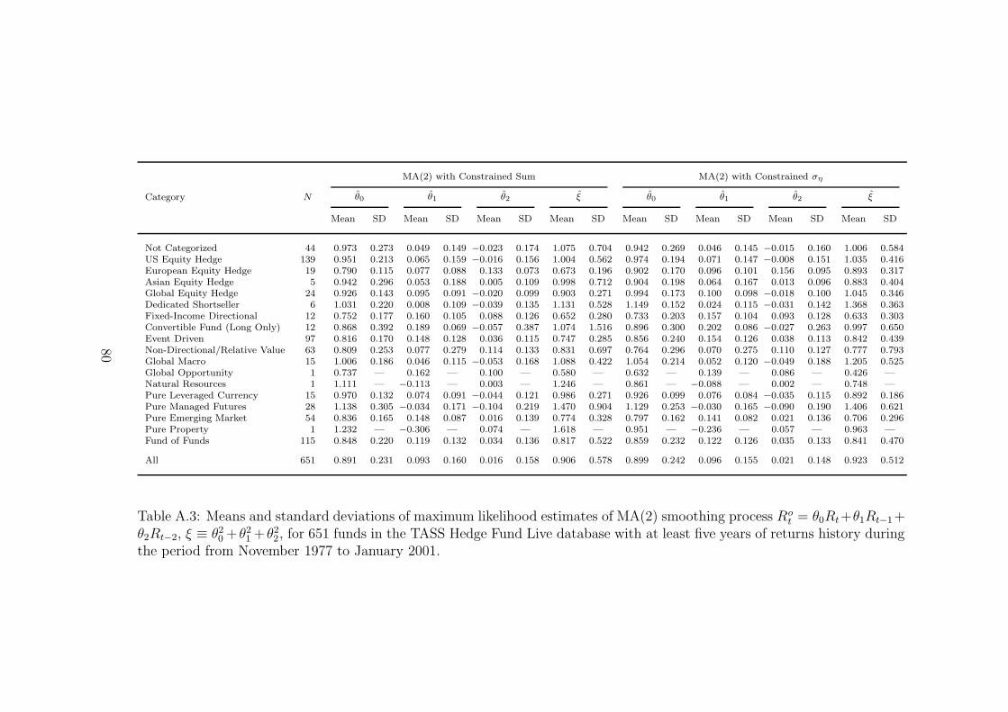
Category N

MA(2) with Constrained Sum MA(2) with Constrained ση

θ0 θ1 θ2 ξ θ0 θ1 θ2 ξ

Mean SD Mean SD Mean SD Mean SD Mean SD Mean SD Mean SD Mean SD

Not Categorized 44 0.973 0.273 0.049 0.149 −0.023 0.174 1.075 0.704 0.942 0.269 0.046 0.145 −0.015 0.160 1.006 0.584US Equity Hedge 139 0.951 0.213 0.065 0.159 −0.016 0.156 1.004 0.562 0.974 0.194 0.071 0.147 −0.008 0.151 1.035 0.416European Equity Hedge 19 0.790 0.115 0.077 0.088 0.133 0.073 0.673 0.196 0.902 0.170 0.096 0.101 0.156 0.095 0.893 0.317Asian Equity Hedge 5 0.942 0.296 0.053 0.188 0.005 0.109 0.998 0.712 0.904 0.198 0.064 0.167 0.013 0.096 0.883 0.404Global Equity Hedge 24 0.926 0.143 0.095 0.091 −0.020 0.099 0.903 0.271 0.994 0.173 0.100 0.098 −0.018 0.100 1.045 0.346Dedicated Shortseller 6 1.031 0.220 0.008 0.109 −0.039 0.135 1.131 0.528 1.149 0.152 0.024 0.115 −0.031 0.142 1.368 0.363Fixed-Income Directional 12 0.752 0.177 0.160 0.105 0.088 0.126 0.652 0.280 0.733 0.203 0.157 0.104 0.093 0.128 0.633 0.303Convertible Fund (Long Only) 12 0.868 0.392 0.189 0.069 −0.057 0.387 1.074 1.516 0.896 0.300 0.202 0.086 −0.027 0.263 0.997 0.650Event Driven 97 0.816 0.170 0.148 0.128 0.036 0.115 0.747 0.285 0.856 0.240 0.154 0.126 0.038 0.113 0.842 0.439Non-Directional/Relative Value 63 0.809 0.253 0.077 0.279 0.114 0.133 0.831 0.697 0.764 0.296 0.070 0.275 0.110 0.127 0.777 0.793Global Macro 15 1.006 0.186 0.046 0.115 −0.053 0.168 1.088 0.422 1.054 0.214 0.052 0.120 −0.049 0.188 1.205 0.525Global Opportunity 1 0.737 — 0.162 — 0.100 — 0.580 — 0.632 — 0.139 — 0.086 — 0.426 —Natural Resources 1 1.111 — −0.113 — 0.003 — 1.246 — 0.861 — −0.088 — 0.002 — 0.748 —Pure Leveraged Currency 15 0.970 0.132 0.074 0.091 −0.044 0.121 0.986 0.271 0.926 0.099 0.076 0.084 −0.035 0.115 0.892 0.186Pure Managed Futures 28 1.138 0.305 −0.034 0.171 −0.104 0.219 1.470 0.904 1.129 0.253 −0.030 0.165 −0.090 0.190 1.406 0.621Pure Emerging Market 54 0.836 0.165 0.148 0.087 0.016 0.139 0.774 0.328 0.797 0.162 0.141 0.082 0.021 0.136 0.706 0.296Pure Property 1 1.232 — −0.306 — 0.074 — 1.618 — 0.951 — −0.236 — 0.057 — 0.963 —Fund of Funds 115 0.848 0.220 0.119 0.132 0.034 0.136 0.817 0.522 0.859 0.232 0.122 0.126 0.035 0.133 0.841 0.470

All 651 0.891 0.231 0.093 0.160 0.016 0.158 0.906 0.578 0.899 0.242 0.096 0.155 0.021 0.148 0.923 0.512

Table A.3: Means and standard deviations of maximum likelihood estimates of MA(2) smoothing process Rot = θ0Rt+θ1Rt−1+

θ2Rt−2, ξ ≡ θ20 + θ2

1 + θ22, for 651 funds in the TASS Hedge Fund Live database with at least five years of returns history during

the period from November 1977 to January 2001.

80

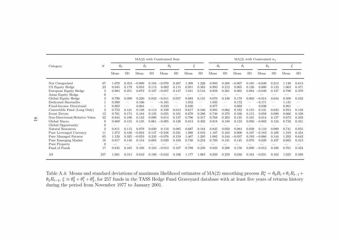
Category N

MA(2) with Constrained Sum MA(2) with Constrained ση

θ0 θ1 θ2 ξ θ0 θ1 θ2 ξ

Mean SD Mean SD Mean SD Mean SD Mean SD Mean SD Mean SD Mean SD

Not Categorized 67 1.079 0.353 −0.009 0.194 −0.070 0.267 1.399 1.226 0.993 0.268 −0.007 0.165 −0.049 0.214 1.130 0.613US Equity Hedge 23 0.945 0.179 0.053 0.113 0.002 0.115 0.951 0.363 0.993 0.212 0.065 0.126 0.000 0.123 1.063 0.471European Equity Hedge 3 0.984 0.251 0.073 0.107 −0.057 0.147 1.041 0.544 0.859 0.201 0.065 0.094 −0.049 0.127 0.788 0.378Asian Equity Hedge 0 — — — — — — — — — — — — — — — —Global Equity Hedge 3 0.790 0.099 0.220 0.043 −0.011 0.057 0.683 0.131 0.670 0.196 0.179 0.003 −0.014 0.044 0.508 0.242Dedicated Shortseller 1 0.999 — 0.166 — −0.165 — 1.052 — 1.035 — 0.172 — −0.171 — 1.131 —Fixed-Income Directional 1 0.902 — 0.064 — 0.033 — 0.820 — 0.977 — 0.069 — 0.036 — 0.961 —Convertible Fund (Long Only) 3 0.753 0.121 0.138 0.113 0.109 0.013 0.617 0.166 0.885 0.062 0.182 0.155 0.131 0.033 0.854 0.158Event Driven 12 0.761 0.174 0.184 0.135 0.055 0.101 0.670 0.286 0.740 0.270 0.166 0.115 0.058 0.099 0.666 0.438Non-Directional/Relative Value 22 0.844 0.196 0.142 0.099 0.014 0.137 0.796 0.317 0.768 0.203 0.135 0.101 0.014 0.127 0.673 0.332Global Macro 9 0.869 0.155 0.135 0.061 −0.005 0.126 0.813 0.302 0.818 0.188 0.123 0.050 −0.002 0.124 0.732 0.351Global Opportunity 0 — — — — — — — — — — — — — — — —Natural Resources 2 0.811 0.115 0.079 0.030 0.110 0.085 0.687 0.164 0.845 0.050 0.084 0.039 0.119 0.099 0.741 0.055Pure Leveraged Currency 11 1.272 0.446 −0.024 0.147 −0.248 0.331 1.980 2.016 1.107 0.163 0.000 0.107 −0.183 0.169 1.319 0.424Pure Managed Futures 65 1.129 0.325 −0.053 0.233 −0.076 0.159 1.467 1.295 1.082 0.244 −0.037 0.193 −0.066 0.144 1.292 0.642Pure Emerging Market 18 0.817 0.148 0.154 0.085 0.029 0.109 0.730 0.254 0.789 0.181 0.145 0.078 0.028 0.107 0.692 0.313Pure Property 0 — — — — — — — — — — — — — — — —Fund of Funds 17 0.845 0.165 0.168 0.103 −0.013 0.107 0.789 0.250 0.823 0.208 0.158 0.090 −0.012 0.106 0.761 0.324

All 257 1.001 0.314 0.042 0.190 −0.042 0.196 1.177 1.064 0.950 0.259 0.046 0.164 −0.031 0.162 1.025 0.569

Table A.4: Means and standard deviations of maximum likelihood estimates of MA(2) smoothing process Rot = θ0Rt+θ1Rt−1+

θ2Rt−2, ξ ≡ θ20 + θ2

1 + θ22, for 257 funds in the TASS Hedge Fund Graveyard database with at least five years of returns history

during the period from November 1977 to January 2001.

81

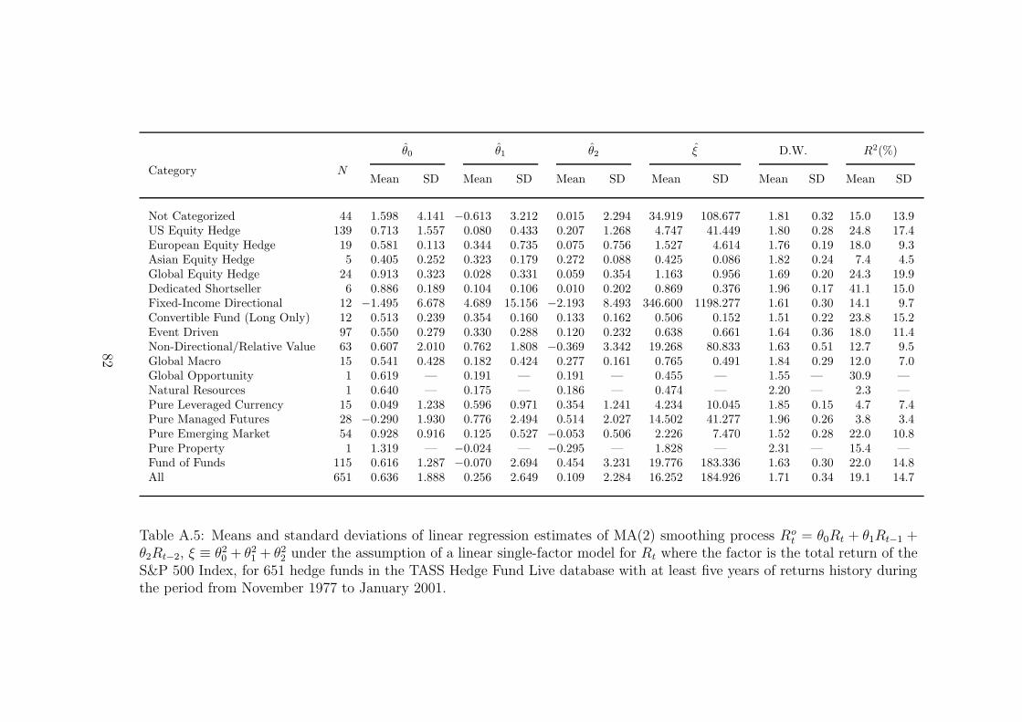
Category N

θ0 θ1 θ2 ξ D.W. R2(%)

Mean SD Mean SD Mean SD Mean SD Mean SD Mean SD

Not Categorized 44 1.598 4.141 −0.613 3.212 0.015 2.294 34.919 108.677 1.81 0.32 15.0 13.9US Equity Hedge 139 0.713 1.557 0.080 0.433 0.207 1.268 4.747 41.449 1.80 0.28 24.8 17.4European Equity Hedge 19 0.581 0.113 0.344 0.735 0.075 0.756 1.527 4.614 1.76 0.19 18.0 9.3Asian Equity Hedge 5 0.405 0.252 0.323 0.179 0.272 0.088 0.425 0.086 1.82 0.24 7.4 4.5Global Equity Hedge 24 0.913 0.323 0.028 0.331 0.059 0.354 1.163 0.956 1.69 0.20 24.3 19.9Dedicated Shortseller 6 0.886 0.189 0.104 0.106 0.010 0.202 0.869 0.376 1.96 0.17 41.1 15.0Fixed-Income Directional 12 −1.495 6.678 4.689 15.156 −2.193 8.493 346.600 1198.277 1.61 0.30 14.1 9.7Convertible Fund (Long Only) 12 0.513 0.239 0.354 0.160 0.133 0.162 0.506 0.152 1.51 0.22 23.8 15.2Event Driven 97 0.550 0.279 0.330 0.288 0.120 0.232 0.638 0.661 1.64 0.36 18.0 11.4Non-Directional/Relative Value 63 0.607 2.010 0.762 1.808 −0.369 3.342 19.268 80.833 1.63 0.51 12.7 9.5Global Macro 15 0.541 0.428 0.182 0.424 0.277 0.161 0.765 0.491 1.84 0.29 12.0 7.0Global Opportunity 1 0.619 — 0.191 — 0.191 — 0.455 — 1.55 — 30.9 —Natural Resources 1 0.640 — 0.175 — 0.186 — 0.474 — 2.20 — 2.3 —Pure Leveraged Currency 15 0.049 1.238 0.596 0.971 0.354 1.241 4.234 10.045 1.85 0.15 4.7 7.4Pure Managed Futures 28 −0.290 1.930 0.776 2.494 0.514 2.027 14.502 41.277 1.96 0.26 3.8 3.4Pure Emerging Market 54 0.928 0.916 0.125 0.527 −0.053 0.506 2.226 7.470 1.52 0.28 22.0 10.8Pure Property 1 1.319 — −0.024 — −0.295 — 1.828 — 2.31 — 15.4 —Fund of Funds 115 0.616 1.287 −0.070 2.694 0.454 3.231 19.776 183.336 1.63 0.30 22.0 14.8All 651 0.636 1.888 0.256 2.649 0.109 2.284 16.252 184.926 1.71 0.34 19.1 14.7

Table A.5: Means and standard deviations of linear regression estimates of MA(2) smoothing process Rot = θ0Rt + θ1Rt−1 +

θ2Rt−2, ξ ≡ θ20 + θ2

1 + θ22 under the assumption of a linear single-factor model for Rt where the factor is the total return of the

S&P 500 Index, for 651 hedge funds in the TASS Hedge Fund Live database with at least five years of returns history duringthe period from November 1977 to January 2001.

82

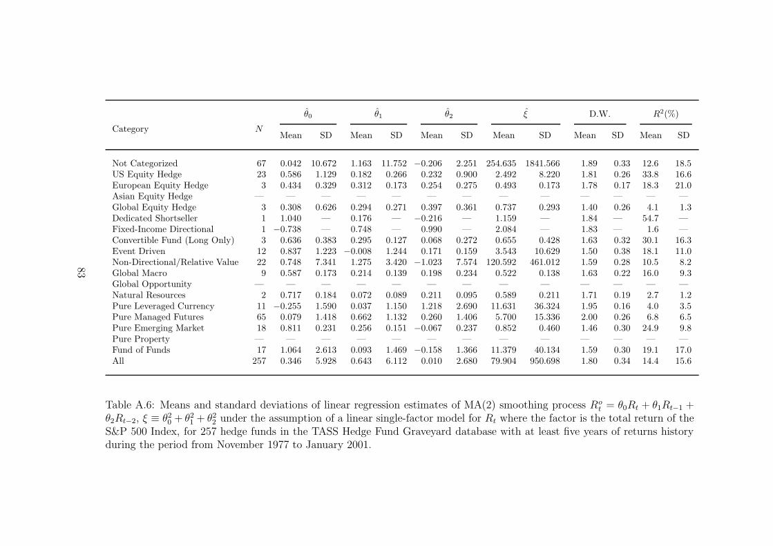
Category N

θ0 θ1 θ2 ξ D.W. R2(%)

Mean SD Mean SD Mean SD Mean SD Mean SD Mean SD

Not Categorized 67 0.042 10.672 1.163 11.752 −0.206 2.251 254.635 1841.566 1.89 0.33 12.6 18.5US Equity Hedge 23 0.586 1.129 0.182 0.266 0.232 0.900 2.492 8.220 1.81 0.26 33.8 16.6European Equity Hedge 3 0.434 0.329 0.312 0.173 0.254 0.275 0.493 0.173 1.78 0.17 18.3 21.0Asian Equity Hedge — — — — — — — — — — — — —Global Equity Hedge 3 0.308 0.626 0.294 0.271 0.397 0.361 0.737 0.293 1.40 0.26 4.1 1.3Dedicated Shortseller 1 1.040 — 0.176 — −0.216 — 1.159 — 1.84 — 54.7 —Fixed-Income Directional 1 −0.738 — 0.748 — 0.990 — 2.084 — 1.83 — 1.6 —Convertible Fund (Long Only) 3 0.636 0.383 0.295 0.127 0.068 0.272 0.655 0.428 1.63 0.32 30.1 16.3Event Driven 12 0.837 1.223 −0.008 1.244 0.171 0.159 3.543 10.629 1.50 0.38 18.1 11.0Non-Directional/Relative Value 22 0.748 7.341 1.275 3.420 −1.023 7.574 120.592 461.012 1.59 0.28 10.5 8.2Global Macro 9 0.587 0.173 0.214 0.139 0.198 0.234 0.522 0.138 1.63 0.22 16.0 9.3Global Opportunity — — — — — — — — — — — — —Natural Resources 2 0.717 0.184 0.072 0.089 0.211 0.095 0.589 0.211 1.71 0.19 2.7 1.2Pure Leveraged Currency 11 −0.255 1.590 0.037 1.150 1.218 2.690 11.631 36.324 1.95 0.16 4.0 3.5Pure Managed Futures 65 0.079 1.418 0.662 1.132 0.260 1.406 5.700 15.336 2.00 0.26 6.8 6.5Pure Emerging Market 18 0.811 0.231 0.256 0.151 −0.067 0.237 0.852 0.460 1.46 0.30 24.9 9.8Pure Property — — — — — — — — — — — — —Fund of Funds 17 1.064 2.613 0.093 1.469 −0.158 1.366 11.379 40.134 1.59 0.30 19.1 17.0All 257 0.346 5.928 0.643 6.112 0.010 2.680 79.904 950.698 1.80 0.34 14.4 15.6

Table A.6: Means and standard deviations of linear regression estimates of MA(2) smoothing process Rot = θ0Rt + θ1Rt−1 +

θ2Rt−2, ξ ≡ θ20 + θ2

1 + θ22 under the assumption of a linear single-factor model for Rt where the factor is the total return of the

S&P 500 Index, for 257 hedge funds in the TASS Hedge Fund Graveyard database with at least five years of returns historyduring the period from November 1977 to January 2001.

83

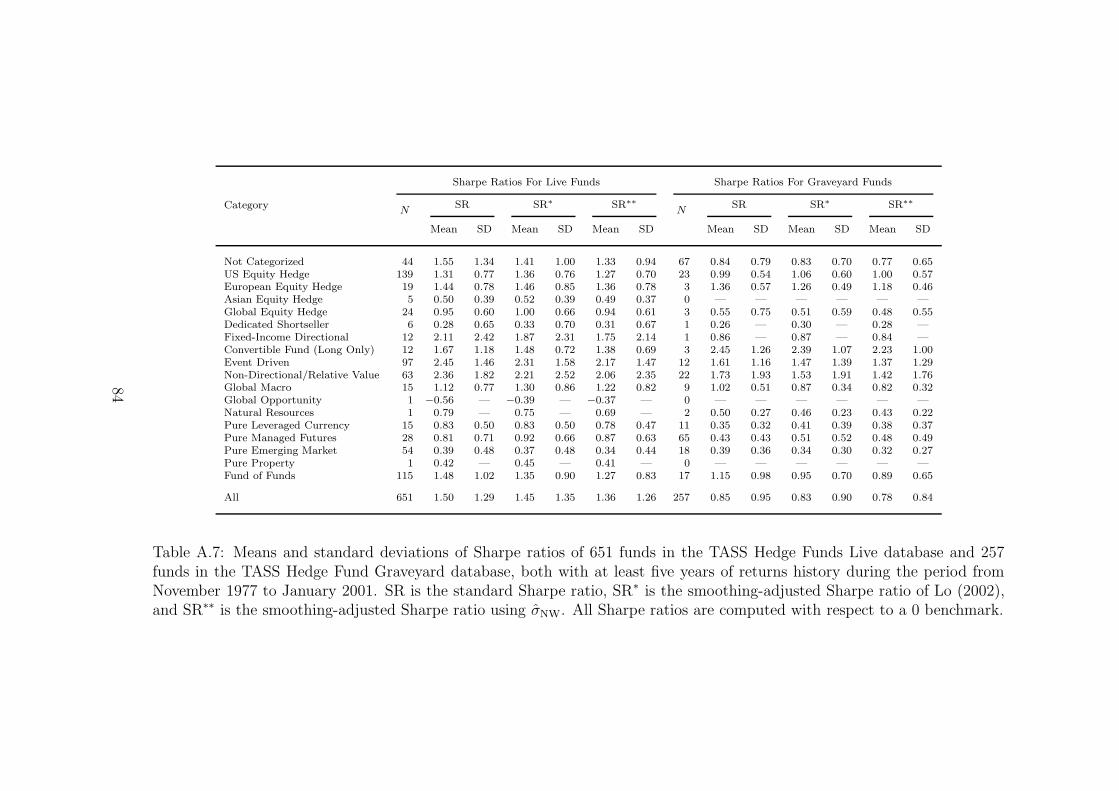
Category

Sharpe Ratios For Live Funds Sharpe Ratios For Graveyard Funds

NSR SR∗ SR∗∗

NSR SR∗ SR∗∗

Mean SD Mean SD Mean SD Mean SD Mean SD Mean SD

Not Categorized 44 1.55 1.34 1.41 1.00 1.33 0.94 67 0.84 0.79 0.83 0.70 0.77 0.65US Equity Hedge 139 1.31 0.77 1.36 0.76 1.27 0.70 23 0.99 0.54 1.06 0.60 1.00 0.57European Equity Hedge 19 1.44 0.78 1.46 0.85 1.36 0.78 3 1.36 0.57 1.26 0.49 1.18 0.46Asian Equity Hedge 5 0.50 0.39 0.52 0.39 0.49 0.37 0 — — — — — —Global Equity Hedge 24 0.95 0.60 1.00 0.66 0.94 0.61 3 0.55 0.75 0.51 0.59 0.48 0.55Dedicated Shortseller 6 0.28 0.65 0.33 0.70 0.31 0.67 1 0.26 — 0.30 — 0.28 —Fixed-Income Directional 12 2.11 2.42 1.87 2.31 1.75 2.14 1 0.86 — 0.87 — 0.84 —Convertible Fund (Long Only) 12 1.67 1.18 1.48 0.72 1.38 0.69 3 2.45 1.26 2.39 1.07 2.23 1.00Event Driven 97 2.45 1.46 2.31 1.58 2.17 1.47 12 1.61 1.16 1.47 1.39 1.37 1.29Non-Directional/Relative Value 63 2.36 1.82 2.21 2.52 2.06 2.35 22 1.73 1.93 1.53 1.91 1.42 1.76Global Macro 15 1.12 0.77 1.30 0.86 1.22 0.82 9 1.02 0.51 0.87 0.34 0.82 0.32Global Opportunity 1 −0.56 — −0.39 — −0.37 — 0 — — — — — —Natural Resources 1 0.79 — 0.75 — 0.69 — 2 0.50 0.27 0.46 0.23 0.43 0.22Pure Leveraged Currency 15 0.83 0.50 0.83 0.50 0.78 0.47 11 0.35 0.32 0.41 0.39 0.38 0.37Pure Managed Futures 28 0.81 0.71 0.92 0.66 0.87 0.63 65 0.43 0.43 0.51 0.52 0.48 0.49Pure Emerging Market 54 0.39 0.48 0.37 0.48 0.34 0.44 18 0.39 0.36 0.34 0.30 0.32 0.27Pure Property 1 0.42 — 0.45 — 0.41 — 0 — — — — — —Fund of Funds 115 1.48 1.02 1.35 0.90 1.27 0.83 17 1.15 0.98 0.95 0.70 0.89 0.65

All 651 1.50 1.29 1.45 1.35 1.36 1.26 257 0.85 0.95 0.83 0.90 0.78 0.84

Table A.7: Means and standard deviations of Sharpe ratios of 651 funds in the TASS Hedge Funds Live database and 257funds in the TASS Hedge Fund Graveyard database, both with at least five years of returns history during the period fromNovember 1977 to January 2001. SR is the standard Sharpe ratio, SR∗ is the smoothing-adjusted Sharpe ratio of Lo (2002),and SR∗∗ is the smoothing-adjusted Sharpe ratio using σNW. All Sharpe ratios are computed with respect to a 0 benchmark.

84

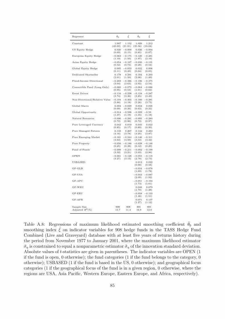
Regressor θ0 ξ θ0 ξ

Constant 1.007 1.152 1.029 1.212(42.02) (21.91) (35.56) (19.04)

US Equity Hedge 0.020 −0.009 0.026 −0.004(0.69) (0.15) (0.85) (0.07)

European Equity Hedge −0.063 −0.175 −0.120 −0.281(1.19) (1.50) (1.97) (2.10)

Asian Equity Hedge −0.054 −0.167 −0.030 −0.131(0.52) (0.73) (0.28) (0.54)

Global Equity Hedge 0.005 −0.053 0.032 0.006(0.11) (0.49) (0.64) (0.05)

Dedicated Shortseller 0.178 0.291 0.184 0.293(2.01) (1.50) (2.06) (1.49)

Fixed-Income Directional −0.203 −0.386 −0.196 −0.375(3.04) (2.63) (2.92) (2.54)

Convertible Fund (Long Only) −0.060 −0.073 −0.064 −0.086(0.95) (0.53) (1.01) (0.62)

Event Driven −0.116 −0.228 −0.124 −0.247(3.74) (3.36) (3.85) (3.49)

Non-Directional/Relative Value −0.194 −0.303 −0.180 −0.281(5.88) (4.18) (5.26) (3.73)

Global Macro 0.004 −0.029 0.034 0.026(0.09) (0.26) (0.63) (0.22)

Global Opportunity −0.314 −0.598 −0.309 −0.59(1.37) (1.19) (1.35) (1.18)

Natural Resources −0.096 −0.281 −0.095 −0.284(0.72) (0.96) (0.72) (0.97)

Pure Leveraged Currency 0.042 0.019 0.045 0.022(0.85) (0.17) (0.89) (0.20)

Pure Managed Futures 0.133 0.267 0.142 0.284(4.16) (3.78) (4.25) (3.87)

Pure Emerging Market −0.161 −0.344 −0.146 −0.311(4.63) (4.50) (3.53) (3.42)

Pure Property −0.056 −0.190 −0.028 −0.146(0.25) (0.38) (0.12) (0.29)

Fund of Funds −0.099 −0.211 −0.092 −0.199(3.32) (3.21) (3.03) (2.96)

OPEN −0.061 −0.128 −0.055 −0.118(3.27) (3.13) (2.78) (2.73)

USBASED 0.012 0.022(0.68) (0.58)

GF-GLB −0.034 −0.078(1.69) (1.78)

GF-USA −0.043 −0.087(2.09) (1.92)

GF-APC −0.051 −0.104(1.73) (1.61)

GF-WEU 0.048 0.079(1.70) (1.28)

GF-EEU −0.058 −0.133(1.46) (1.51)

GF-AFR 0.071 0.137(1.27) (1.12)

Sample Size 908 908 891 891

Adjusted R2(%) 15.7 11.4 16.9 12.6

Table A.8: Regressions of maximum likelihood estimated smoothing coefficient θ0 andsmoothing index ξ on indicator variables for 908 hedge funds in the TASS Hedge FundCombined (Live and Graveyard) database with at least five years of returns history duringthe period from November 1977 to January 2001, where the maximum likelihood estimatorση is constrained to equal a nonparametric estimator ση of the innovation standard deviation.Absolute values of t-statistics are given in parentheses. The indicator variables are OPEN (1if the fund is open, 0 otherwise); the fund categories (1 if the fund belongs to the category, 0otherwise); USBASED (1 if the fund is based in the US, 0 otherwise); and geographical focuscategories (1 if the geographical focus of the fund is in a given region, 0 otherwise, where theregions are USA, Asia Pacific, Western Europe, Eastern Europe, and Africa, respectively).

85

References

Ackermann, C., McEnally, R. and D. Ravenscraft, 1999, “The Performance of Hedge Funds:Risk, Return, and Incentives”, Journal of Finance 54, 833–874.

Agarwal, V. and N. Naik, 2000a, “Performance Evaluation of Hedge Funds with Buy-and-Hold and Option-Based Strategies”, Hedge Fund Centre Working Paper No. HF–003,London Business School.

Agarwal, V. and N. Naik, 2000b, “On Taking the ”Alternative” Route: The Risks, Rewards,and Performance Persistence of Hedge Funds”, Journal of Alternative Investments 2,6–23.

Agarwal, V. and N. Naik, 2000c, “Multi-Period Performance Persistence Analysis of HedgeFunds Source”, Journal of Financial and Quantitative Analysis 35, 327–342.

Agarwal, V. and N. Naik, 2002, “Risks and Portfolio Decisions Involving Hedge Funds”,Institute of Finance and Accounting Working Paper No. 364, London Business School.

Asness, C., Krail, R. and J. Liew, 2001, “Do Hedge Funds Hedge?”, The Journal of PortfolioManagement 28, 6–19.

Atchison, M., K. Butler, and R. Simonds, 1987, “Nonsynchronous Security Trading andMarket Index Autocorrelation”, Journal of Finance 42, 111–118.

Baquero, G., Horst, J. and M. Verbeek, 2002, ”Survival, Look-Ahead Bias and the Perfor-mance of Hedge Funds”, Erasmus University Rotterdam Working Paper.

Bhargava, R., Bose, A. and D. Dubofsky, 1998, “Exploiting International Stock Market Cor-relations with Open-End International Mutual Funds”, Journal of Business, Finance,and Accounting 25, 765–773.

Bhattacharya, S. and P. Pfleiderer, 1985, “Delegated Portfolio Management”, Journal ofEconomic Theory 36, 1–25.

Beneish, M., 2001, “Earnings Management: A Perspective”, Managerial Finance 27, 3–17.

Billingsley, P., 1968, Convergence of Probability Measures. New York: John Wiley andSons.

Black, F., 1986, “Noise”, Journal of Finance 41, 529–544.

Boudoukh, J., Richardson, M., Subrahmanyam, M. and R. Whitelaw, 2002, “Stale Pricesand Strategies for Trading Mutual Funds”, Financial Analysts Journal 58, 53–71.

Brockwell, P., and R. Davis, 1991, Time Series: Theory and Methods, Second Edition. NewYork: Springer-Verlag.

Brown, S. and W. Goetzmann, 2001, “Hedge Funds With Style”, NBER Working PaperNo. 8173.

Brown, S., Goetzmann, W., Ibbotson, R. and S. Ross, 1992, “Survivorship Bias in Perfor-mance Studies”, Review of Financial Studies 5, 553–580.

86

Brown, S., Goetzmann, W. and R. Ibbotson, 1999, “Offshore Hedge Funds: Survival andPerformance 1989–1995”, Journal of Business 72, 91–118.

Brown, S., Goetzmann, W. and B. Liang, 2002, “Fees on Fees in Funds of Funds”, YaleICF Work Paper No. 02–33.

Brown, S., Goetzmann, W. and J. Park, 1997, “Conditions for Survival: Changing Riskand the Performance of Hedge Fund Managers and CTAs”, Yale School of ManagementWork Paper No. F–59.

Brown, S., Goetzmann, W. and J. Park, 2000, “Hedge Funds and the Asian CurrencyCrisis”, Journal of Portfolio Management 26, 95–101.

Brown, S., Goetzmann, W. and J. Park, 2001, “Careers and Survival: Competition andRisks in the Hedge Fund and CTA Industry”, Journal of Finance 56, 1869–1886.

Campbell, J., Lo, A., and C. MacKinlay, 1997, The Econometrics of Financial Markets.Princeton, NJ: Princeton University Press.

Carpenter, J., 2000, “Does Option Compensation Increase Managerial Risk Appetite?”,Journal of Finance 55, 2311–2331.

Carpenter, J., Dybvig, P. and H. Farnsworth, 2001, “Portfolio Performance and Agency”,unpublished working paper, Stern School of Business, New York University.

Carpenter, J. and A. Lynch, 1999, “Survivorship Bias and Attrition Effects in Measures ofPerformance Persistence”, Journal of Financial Economics 54, 337–374.

Cecchetti, S. and N. Mark, 1990, “Evaluating Empirical Tests of Asset Pricing Models”,American Economic Review 80, 48–51.

Chalmers, J., Edelen, R. and G. Kadlec, 2001, “On the Perils of Security Pricing by Fi-nancial Intermediaries: The Wildcard Option in Transacting Mutual-Fund Shares”,Journal of Finance 56, 2209–2236.

Chandar, N. and R. Bricker, 2002, “Incentives, Discretion, and Asset Valuation in Closed-End Mutual Funds”, Journal of Accounting Research 40, 1037–1070.

Cohen, K., Hawawini, G., Maier, S., Schwartz, R. and D. Whitcomb, 1983a, ”Estimatingand Adjusting for the Intervalling-Effect Bias in Beta,” Management Science 29, 135–148.

Cohen, K., Hawawini, G, Maier, S., Schwartz, R. and D. Whitcomb, 1983b, “Friction inthe Trading Process and the Estimation of Systematic Risk”, Journal of FinancialEconomics 12, 263–278.

Cohen, K., Maier, S., Schwartz, R. and D. Whitcomb, 1978, “The Returns GenerationProcess, Returns Variance, and the Effect of Thinness in Securities Markets”, Journalof Finance 33, 149–167.

Cohen, K., Maier, S, Schwartz, R. and D. Whitcomb, 1979, “On the Existence of Serial Cor-relation in an Efficient Securities Market”, TIMS Studies in the Management Sciences11, 151–168.

Cohen, K., Maier, S., Schwartz, R. and D. Whitcomb, 1986, The Microstructure of Securi-ties Markets. Englewood Cliffs, NJ: Prentice Hall.

87

Dimson, E., 1979, “Risk Measurement When Shares Are Subject to Infrequent Trading”,Journal of Financial Economics 7, 197–226.

Edwards, F., and M. Caglayan, 2001, “Hedge Fund and Commodity Fund Investments inBull and Bear Markets”, The Journal of Portfolio Management 27, 97–108.

Elton, E. and M. Gruber, 2002, “Incentive Fees and Mutual Funds”, to appear in Journalof Finance.

Fama, E., 1970, “Efficient Capital Markets: A Review of Theory and Empirical Work”,Journal of Finance 25, 383–417.

Farmer, D., 1998, “Market Force, Ecology, and Evolution”, Santa Fe Institute WorkingPaper No. 98–12-118.

Farmer, D. and A. Lo, 1999, “Frontiers of Finance: Evolution and Efficient Markets”,Proceedings of the National Academy of Sciences 96, 9991–9992.

Fisher, J., Geltner, D. and R. Webb, 1994, “Value Indices of Commercial Real Estate:A Comparison of Index Construction Methods”, Journal of Real Estate Finance andEconomics 9, 137–164.

Fisher, J., Gatzlaff, D., Geltner, D. and D. Haurin, 2003, “Controlling for the Impact ofVariable Liquidity in Commercial Real Estate Price Indices”, Real Estate Economics31, 269–303.

Fisher, L., 1966, “Some New Stock Market Indexes”, Journal of Business 39, 191–225.

Fung, W. and D. Hsieh, 1997a, “Empirical Characteristics of Dynamic Trading Strategies:The Case of Hedge Funds”, Review of Financial Studies 10, 275–302.

Fung, W. and D. Hsieh, 1997b, “Investment Style and Survivorship Bias in the Returns ofCTAs: The Information Content of Track Records”, Journal of Portfolio Management24, 30–41.

Fung, W. and D. Hsieh, 1999, “A Primer on Hedge Funds”, Journal of Empirical Finance6, 309–31.

Fung, W. and D. Hsieh, 2000, “Performance Characteristics of Hedge Funds and Commod-ity Funds: Natural versus Spurious Biases”, Journal of Financial and QuantitativeAnalysis 35, 291–307.

Fung, W. and D. Hsieh, 2001, “The Risk in Hedge Fund Strategies: Theory and Evidencefrom Trend Followers”, Review of Financial Studies 14, 313–341.

Fung, W. and D. Hsieh, 2002, “Asset-Based Style Factors for Hedge Funds”, FinancialAnalysts Journal 58, 16–27.

Getmansky, M. and A. Lo, 2003, “A System Dynamics Model of the Hedge Fund Industry”,unpublished working paper, MIT Laboratory for Financial Engineering.

Goetzmann, W., Ingersoll, J. and S. Ross, 1997, “High Water Marks and Hedge FundManagement Contracts”, to appear in Journal of Finance.

Goetzmann, W., Ingersoll, J., Spiegel, M. and I. Welch, 2002, “Sharpening Sharpe Ratios”,National Bureau of Economic Research Working Paper No. W9116.

88

Goetzmann, W., Ivkovic, Z. and G. Rouwenhorst, 1999, “Day Trading International MutualFunds: Evidence and Policy Solutions”, Journal of Financial and Quantitative Analysis36, 287–309.

Goodwin, T., 1993, “Business-Cycle Analysis with a Markov-Switching Model”, Journal ofBusiness and Economic Statistics 11, 331–339.

Granger, C., 1980, “Long Memory Relations and the Aggregation of Dynamic Models”,Journal of Econometrics 14, 227–238.

Granger, C., 1988, “Aggregation of Time Series Variables—A Survey”, Federal ReserveBank of Minneapolis Institute for Empirical Macroeconomics, Discussion Paper 1.

Greene, J. and C. Hodges, 2002, “The Dilution Impact of Daily Fund Flows on Open-EndMutual Funds”, Journal of Financial Economics 65, 131–158.

Grossman, S., 1976, “On The Efficiency of Competitive Stock Markets Where Trades HaveDiverse Information”, Journal of Finance 31, 573–585.

Grossman, S. and J. Stiglitz, 1980, “On the Impossibility of Informationally Efficient Mar-kets”, American Economic Review 70, 393–408.

Gyourko, J. and D. Keim, 1992, “What Does the Stock Market Tell Us About Real EstateReturns”, AREUEA Journal 20, 457–486.

Hamilton, J., 1989, “A New Approach to the Economic Analysis of Nonstationary TimeSeries and the Business Cycle”, Econometrica 57, 357–384.

Hamilton, J., 1990, “Analysis of Time Series Subject to Changes in Regime”, Journal ofEconometrics 45, 39–70.

Hamilton, J., 1996, “Specification Testing in Markov-Switching Time Series Models”, Jour-nal of Econometrics 70, 127–157.

Hansen, L., 1982, “Large Sample Properties of Generalized Method of Moments Estima-tors”, Econometrica 50, 1029–1054.

Healy, P. and J. Wahlen, 1999, “A Review of the Earnings Management Literature and ItsImplications for Standard Setting”, Accounting Horizons 14, 365–383.

Hendricks, D., Patel, J. and R. Zeckhauser, 1997, “The J-Shape of Performance PersistenceGiven Survivorship Bias”, Review of Economics and Statistics 79, 161–170.

Herrndorf, N., 1984, “A Functional Central Limit Theorem For Weakly Dependent Se-quences of Random Variables”, Annals of Probability 12, 141–153.

Horst, J., Nijman, T. and M. Verbeek, 2001, “Eliminating Look-Ahead Bias in EvaluatingPersistence in Mutual Fund Performance”, Journal of Empirical Finance 8, 345–373.

Jobson, J. and R. Korkie, 1981, “Performance Hypothesis Testing with the Sharpe andTreynor Measures”, Journal of Finance 36, 889–908.

Kadlec, G. and D. Patterson, 1999, “A Transactions Data Analysis of NonsynchronousTrading”, Review of Financial Studies 12, 609–630.

Kandel, S. and R. Stambaugh, 1991, “Asset Returns and Intertemporal Preferences”, Jour-nal of Monetary Economics 27, 39–71.

89

Kao, D., 2002, “Battle for Alphas: Hedge Funds versus Long-Only Portfolios”, FinancialAnalysts Journal 58, 16–36.

Leroy, S., 1973, “Risk Aversion and the Martingale Property of Stock Returns”, Interna-tional Economic Review 14, 436–446.

Liang, B., 1999, “On the Performance of Hedge Funds”, Financial Analysts Journal 55,72–85.

Liang, B., 2000, “Hedge Funds: The Living and the Dead”, Journal of Financial andQuantitative Analysis 35, 309–326.

Liang, B., 2001, “Hedge Fund Performance: 1990–1999”, Financial Analysts Journal 57,11–18.

Lo, A., 2001, “Risk Management For Hedge Funds: Introduction and Overview”, to appearin Financial Analysts Journal 57, 16–33.

Lo, A., 2002, “The Statistics of Sharpe Ratios”, Financial Analysts Journal 58, 36–50.

Lo, A. and C. MacKinlay, 1988, “Stock Market Prices Do Not Follow Random Walks:Evidence from a Simple Specification Test”, Review of Financial Studies 1, 41–66.

Lo, A. and C. MacKinlay, 1990, “An Econometric Analysis of Nonsynchronous Trading”,Journal of Econometrics 45, 181–212.

Lo, A. and C. MacKinlay, 1999, A Non-Random Walk Down Wall Street. Princeton, NJ:Princeton University Press.

Lochoff, R., 2002, “Hedge Funds and Hope”, The Journal of Portfolio Management 28,92–99.

Lucas, R., 1978, “Asset Prices in an Exchange Economy”, Econometrica 46, 1429–1446.

Newey, W. and K. West, 1987, “A Simple Positive Definite Heteroscedasticity and Auto-correlation Consistent Covariance Matrix”, Econometrica 55, 703–705.

Niederhoffer, V., 1998, The Education of a Speculator. New York: John Wiley & Sons.

Richardson, M. and J. Stock, 1989, “Drawing Inferences from Statistics Based on MultiyearAsset Returns”, Journal of Financial Economics 25, 323–348.

Ross, S. and R. Zisler, 1991, “Risk and Return in Real Estate”, Journal of Real EstateFinance and Economics 4, 175–190.

Rubinstein, M., 1976, “The Valuation of Uncertain Income Streams and the Pricing ofOptions”, Bell Journal of Economics 7, 407–425.

Samuelson, P., 1941, “Conditions that the Roots of a Polynomial Be Less than Unity inAbsolute Value”, Annals of mathematical Statistics 45, 689–693.

Samuelson, P., 1965, “Proof that Properly Anticipated Prices Fluctuate Randomly”, In-dustrial Management Review 6, 41–49.

Schneeweis, T. and R. Spurgin, 1996, “Survivor Bias in Commodity Trading Advisor Per-formance”, Journal of Futures Markets 16, 757–772.

90

Scholes, M., and J. Williams, 1977, “Estimating Betas from Nonsynchronous Data”, Journalof Financial Economics 5, 309–328.

Schwert, G., 1977, “Stock Exchange Seats as Capital Assets”, Journal of Financial Eco-nomics 4, 51–78.

Shanken, J., 1987, ”Nonsynchronous Data and the Covariance-Factor Structure of Returns,”Journal of Finance 42, 221–232.

Sharpe, W., 1994, “The Sharpe Ratio”, Journal of Portfolio Management 21, 49–58.

Spurgin, R., 2001, “How to Game Your Sharpe Ratio”, The Journal of Alternative Invest-ments 4, 38–46.

Turner, C., Startz, R. and C. Nelson, 1989, “A Markov Model of Heteroskedasticity, Risk,and Learning in the Stock Market”, Journal of Financial Economics 25, 3–22.

Weisman, A., 2002, “Informationless Investing and Hedge Fund Performance MeasurementBias”, The Journal of Portfolio Management 28, 80–91.

Working, H., 1960, “Note on the Correlation of First Differences of Averages in a RandomChain”, Econometrica 28, 916–918.

91