Department of Economics and Finance

Working Paper No. 09-35

http://www.brunel.ac.uk/about/acad/sss/depts/economics

Econ

omic

s an

d Fi

nanc

e W

orki

ng P

aper

Ser

ies

Guglielmo Maria Caporale, Burcu Erdogan and Vladimir Kuzin

Testing for Convergence in Stock Markets: A Non-linear Factor Approach

September 2009

TESTING FOR CONVERGENCE IN STOCK MARKETS:

A NON-LINEAR FACTOR APPROACH

Guglielmo Maria Caporale Brunel University (London), CESifo and DIW Berlin

Burcu Erdogan

DIW Berlin

Vladimir Kuzin DIW Berlin

September 2009

Abstract

This paper applies the Phillips and Sul (2007) method to test for convergence in stock returns to an extensive dataset including monthly stock price indices for five EU countries (Germany, France, the Netherlands, Ireland and the UK) as well as the US over the period 1973-2008. We carry out the analysis on both sectors and individual industries within sectors. As a first step, we use the Stock and Watson (1998) procedure to filter the data in order to extract the long-run component of the series; then, following Phillips and Sul (2007), we estimate the relative transition parameters. In the case of sectoral indices we find convergence in the middle of the sample period, followed by divergence, and detect four (two large and two small) clusters. The analysis at a disaggregate, industry level again points to convergence in the middle of the sample, and subsequent divergence, but a much larger number of clusters is now found. Splitting the cross-section into two subgroups including Euro area countries, the UK and the US respectively, provides evidence of a global convergence/divergence process not obviously influenced by EU policies.

JEL classification codes: C32, C33, G11, G15 Keywords: Stock Market, Financial Integration, European Monetary Union Convergence, Factor Model Corresponding author: Professor Guglielmo Maria Caporale, Centre for Empirical Finance, Brunel University, West London, UB8 3PH, UK. Tel.: +44 (0)1895 266713. Fax: +44 (0)1895 269770. Email: Guglielmo-Maria.Caporale@brunel.ac.uk

1

1. Introduction Financial integration is an issue which has been extensively investigated in the

literature, recently with an increasing focus on the European case, as the EU has put

considerable emphasis on achieving a higher degree of convergence of financial

markets in its member states. Several different approaches have been taken to

establish whether or not such convergence has taken place or at least whether the

process is under way. Most of these methods rely on rather restrictive assumptions

about the properties of the series being analysed and the type of convergence which

might occur.

This paper exploits some recent developments in the econometrics literature which

provide a more flexible framework for the analysis. Specifically, it applies the Phillips

and Sul (2007) method to test for convergence of stock returns to an extensive dataset

including monthly stock price indices for five EU countries (Germany, France, the

Netherlands, Ireland and the UK) as well as the US over the period 1973m1-2008m8.

This approach has several advantages over others previously used in the literature, as

it does not require stationarity and it is general enough to cover a wide range of

convergence processes. We carry out the analysis on both sectors (35 cross-section

units as a whole) and individual industries within sectors (overall, 119 cross-section

units, see Appendix A for details). The data source is Datastream. As a first step, we

use the Stock and Watson (1998) procedure to filter the data in order to extract the

long-run component of the series; then, following Phillips and Sul (2007), we estimate

the relative transition parameters.

To preview the main results, in the case of sectoral indices we find convergence in the

middle of the sample period, followed by divergence, and detect four (two large and

two small) clusters. The analysis at disaggregate, industry level, again points to

convergence in the middle of the sample, and subsequent divergence, but a much

larger number of clusters is now found. Splitting the cross-section into two subgroups

including the Euro area countries, and both the UK and the US respectively, provides

evidence of a global convergence/divergence process not clearly affected by EU

policies.

2

We try to rationalise these results on the basis of the country versus industry effects

literature, and consider their implications for portfolio management strategies.

Traditionally, a top-down approach has been followed in selecting portfolios, i.e. a

country is chosen first, and stocks within that market are then selected. Such a

strategy is effective if country effects are the main driving force of stock returns.

However, it might have to be revised if industry effects are shown to have become

more important over time. Our clustering results combined with correlation analysis

of stock index returns imply that indeed the relative weight of industry effects has

increased over time, and therefore a traditional top-down investment strategy might

not be effective any longer.

The remainder of the paper is organised as follows. Section 2 briefly reviews the

existing literature on (European) stock market integration. Section 3 outlines the

Phillips and Sul (2007) method. Section 4 presents the empirical results and provides

some interpretation. Section 5 offers some concluding remarks.

2. Literature Review

European financial integration is a topic of extreme interest both to portfolio

managers and policy-makers. The creation of a single market, and then the

introduction of the euro, together with the adoption of various measures promoting

financial integration, are all thought to have resulted in less segmented financial

markets. Obviously, this is a gradual process, which takes time to complete, as many

obstacles to integration have had to be removed over the years. EU countries still have

national stock markets and numerous derivatives markets, cross-border transactions

are still much more expensive than domestic ones (see, e.g., Adjaoute et al., 2000),

taxation, reporting and accounting standards have not been harmonized across

member states. Further, although the introduction of the euro has eliminated currency

risk as a risk factor for portfolio investors, home bias might still persist to some

extent. As a result, full financial integration has yet to be achieved, and clearly the EU

is a considerably less homogeneous financial area compared with the US. However,

ever-increasing (and eventually full) integration has been a top priority for the EU,

and one would expect substantial progress to have been made and significant

convergence to have occurred already.

3

The question arises how one could measure the degree of stock market integration

and/or convergence, and whether global or local risk factors determine returns. In

principle both price-based and quantity-based indicators could be appropriate.

Measures obtained from asset prices models have the disadvantage that these are

difficult to estimate and require specific assumptions (see, e.g., Bekaert and Harvey,

1995). Nevertheless, some studies have taken this approach - for instance,

Hardouvelis et al. (2007), who report a lower cost of capital reflecting higher financial

integration in Europe. Chen and Knez (1995) put forward a general arbitrage

approach which does not require specifying an asset model, but is not, however, very

informative about the convergence process. This has been applied by researchers such

as Fratzscher (2002), who reported increasing correlations across European stock

markets. Ayuso and Blanco (1999) have suggested a refinement of this approach

based on a no-arbitrage condition; they also find increasing global financial

integration in the 1990s.

Correlations are often found to be time-varying and increasing in periods of higher

economic and financial integration (see Goetzmann et al., 2005). Low correlations

between stock markets could be due to a number of reasons, i.e. the already

mentioned home bias, country-specific factors (such as policy framework, legislation

etc.), differences in the pricing of risk, and possibly in the composition of indices. An

alternative explanation for convergence patterns in stock markets could be based on

changes over time in the relative importance of industry and country effects as driving

forces of stock returns1, as�suggested by Ferreira and Ferreira (2006), with important

implications for the gains from international portfolio diversification. In particular,

these authors investigate whether lower cross-country correlations reflect differences

in the composition of indices across countries. Specifically, they use a sample of 10

industry indices in 11 EMU countries and estimate the model proposed by Heston and

Rouwenhorst (1994) to decompose the return of a given stock or industry index into a

common factor, an industry effect and a firm specific disturbance. They find that,

although country effects are still predominant, overtime industry effects have become

1 This topic has been of interest to scholars for a long time indeed. Lessard (1973) has shown with a single-factor model that only a small proportion of the variance of national portfolios is common in an international context which gives rise to considerable risk reduction through the international dimension. He also argues that the industry dimension is much less important than the national dimension in defining groups of securities that share common return elements from 1959 to 1972.

4

increasingly important. This implies that international portfolio diversification across

countries is still a more effective tool for risk reduction than industry diversification

within a country, but increasingly less so. Baca et al. (2000) and Cavaglia et al. (2000)

also reach the conclusion that the importance of industry factors increased towards the

late 1990s. However, Brooks and Del Negro (2004) argue that higher correlations

across national stock markets were a temporary phenomenon, explained by the IT

bubble, following which diversification across countries might still work better.

Another study by Adjaoute and Danthine (2003) simply calculates the cross-sectional

dispersion in country and sector returns respectively and also finds that the benefits

from diversification across sectors have become greater since the end of the1990s.

Baele et al. (2004) use Hodrick-Prescott filtered dispersion series in order to focus on

the slowly moving component, and conclude that country dispersion in the euro area

has been higher than sector dispersion (i.e., cross-country correlations were typically

lower than cross-sector correlations). However, their measure of sector dispersion

surpassed that of country dispersion in 2000, consistently with a possible shift in the

asset allocation paradigm from country-based to sector-based strategies. They also

note that diversifying portfolios across both countries and sectors still yields the

greatest risk reduction. Ferreira and Gama (2005) use a volatility decomposition

method to study the time series behaviour of equity volatility at the world, country

and local industry levels for the most developed21 stock markets. Their findings

suggest that industry diversification became a more effective tool for risk reduction

than geographic diversification in the late 1990s, since industry volatility has been

rising relative to country volatility and correlations among local industries have

declined globally.

The economic interpretation of ex-post correlations of stock market returns, however,

is questionable. Therefore, quantity-based measures such as the shares of equities

managed by equity funds with an international investment strategy are recommended

by authors such as Adam et al. (2002). Baele et al. (2004) update their results

considering investment funds, pension funds and the insurance industry, and again

find evidence of a decrease in the home bias and a rising degree of stock market

integration. They also use a news-based measure of financial integration to establish

whether the sensitivities of country returns to shocks (the ”betas”) have changed over

time in response to deeper economic and monetary integration, and conclude that the

5

degree of integration has increased both within the euro area and globally, and

especially so in the former.

In the last two decades a new literature has also developed based on the concepts of β-

and σ-convergence introduced by Barro and Sala-i-Martin (1991, 1992). Presence of

β-convergence implies mean reversion for the panel units, whilst σ-convergence is a

reduction in overall cross-section dispersion. Islam (2003) shows that β-convergence

is a necessary but not sufficient condition for σ-convergence, but has a more natural

interpretation inthe context of growth models. He also points out some problems

arising when testing convergence empirically (see also Durlauf and Quah, 1999 and

Bernard and Durlauf, 1996). First, the implications of growth models for absolute

convergence and convergence „clubs” are not clear (for alternative testing methods,

see Hobijn and Franses, 2000, and Busetti et al., 2006). Second, different tests do not

have the same null hypothesis and therefore are not directly comparable. Third, most

tests are based on rather specific and restrictive assumptions about the underlying

panel structures.

A new approach which overcomes these difficulties has recently been introduced by

Phillips and Sul (2007). Theirs is a ”non-linear, time-varying coefficient factor

model” with well-defined asymptotic properties. A regression-based test is proposed,

together with a clustering procedure. This approach is not dependent on stationarity

assumptions and allows for a wide variety of possible transition paths towards

convergence (including subgroup convergence). Moreover, the same test is applied

for overall convergence and clustering. Fritsche and Kuzin (2008) apply this method

to investigate convergence in European prices, unit labour costs, income and

productivity over the period 1960-2006and find different transition paths of

convergence as well as regional clusters.

In the next section we outline this procedure, which is then applied to analyse

convergence in European and US stock markets in Section 4.

6

3. Non-Linear Factor Analysis

Model Factor analysis is an important tool for analysing datasets with large time

series and cross-section dimensions, since it allows to decompose series into common

and country-specific components in a very parsimonious way. A simplest example is

a linear factor model, which has the following form

,it it itX δ ε= + (1)

for i = 1, . . . ,N and t = 1, . . . , T, where Xit are observable series and μt as well as εit

unobservable components. In many cases unobservable components can be easily

estimated using the method of principal components and the asymptotic properties of

estimators are well defined for large N and T (see Bai, 2003).

However, the loading coefficients δi are assumed to be time invariant in (1) and for

the country-specific components εit stationarity or at least difference-stationarity

properties are required. As long as convergence is understood as a non-stationary

process, such as σ-convergence (Barro and Sala-i-Martin, 1991, 1992), analysing it

proves to be problematic in this framework. Phillips and Sul (2007) adopt a different

specification from (1) and allow for time-variation in the loading coefficients as

follows

,it it tX δ μ= (2)

where δit absorbs the idiosyncratic component εit. Next, non-stationary transitional

behaviour of factor loadings is proposed, so that each coefficient converges to some

unit specific constant: 1( ) .it i it it L t t αδ δ σ ξ − −= + (3)

The stochastic component declines asymptotically since ξit is assumed to be

independent across i and weakly dependent over t, and L(t) is a slowly varying

function, i.e. L(t) = log t. Obviously, for all α ≥ 0 the loadings δit converge to δi

enabling one to consider statistical hypotheses of convergence in the observed panel

Xit. In particular, the null of convergence is formulated as follows

H0 : δit → δ for all δ and α ≥ 0.

Transition paths The central issue of the proposed approach is the estimation of the

time-varying loadings δit. Phillips and Sul (2007) suggest a simple non-parametric

way to extract information about δit by using their relative versions - the so-called

relative transition parameters:

7

1 1

.1 1it it

it N Nit iti i

XhX

N N

δ

δ= =

= =∑ ∑

(4)

Provided that the panel average 1

1 Niti

XN =∑ is not zero, the relative transition

parameters measure δit in relation to the panel average at time t and describe the

transition path of unit i. Obviously, if all loadings converge to the same value δit → δ,

the relative transition parameters converge to one, hit → 1, so that the cross-sectional

variance goes to zero. Based on this property the following convergence testing

procedure was proposed by Phillips and Sul (2007).

Testing First, a measure for the cross-sectional dispersion of the relative transition

parameters relative to one is calculated:

21

1 ( 1) .Nit iti

H hN =

= −∑ (5)

Second, the following OLS regression is performed: ^ ^ ^

1log( / ) 2 log logt t tH H L a b t u− = + + (6)

for t = [rT], [rT] + 1, . . . , T with some r > 0. As in the previous case, L(t) denotes

some slowly varying function, where L(t) = log(t + 1) turns out to be simplest and

obvious choice. The convergence speed α is estimated by^ ^

2b α= . It is important,

since the focus is on convergence as the sample gets larger, to discard the first [rT]-1

observations. The choice of the subsample to be discarded plays an important role,

because both the limit distribution and the power properties of the procedure depend

on it. Phillips and Sul (2007) suggest r = 0.3 based on their simulation experiments.

Finally, the regression coeffcient ^b is tested under the one-sided null hypothesis α ≥ 0

and using a HAC standard error. Under some regularity conditions stated in Phillips

and Sul (2007) the test statistic ^b

t is asymptotically standard normally distributed, so

that standard critical values can be employed. The null is rejected for large negative

values of ^b

t .

Clusters Rejecting the null of convergence does not mean that each unit in the panel

follows only its own independent path. Obviously, subgroups can also converge and

8

build convergence clubs. Accordingly, Phillips and Sul (2007) also propose an

algorithm for sorting units into converging clusters given some statistical significance

values. The algorithm is based on the logarithmic regression (6) and consists of four

steps, which are repeated until all units are sorted into cluster formations (see Phillips

and Sul, 2007, for details). Two critical values need to be fed into the procedure in

order to run it: one for testing a given subgroup for convergence, set to the standard -

1.65 in the following analysis, and the other for testing if a particular unit belongs to a

given group. Phillips and Sul (2007) argue in favour of a much strict setting for the

second value: they suggest using a zero threshold and even increasing it, if the null for

the whole subgroup is rejected in subsequent steps. The procedure possesses great

flexibility enabling one to identify cluster formations with all possible configurations:

overall convergence, overall divergence, converging subgroups and single diverging

units.

Filtering However, in many economic applications the underlying time series often

contain short-run components, i.e. business cycle comovements, which render

representation (2) inappropriate. Equation (2) can be extended by adding a unit-

specific additive short-run component:

.it it t itX δ μ κ= + (7)

Any subsequent convergence analysis is eventually distorted by these additive

components; so that some filtering techniques are necessary to extract the long-run

components .it tδ μ The particular filtering techniques applied in this paper are

discussed in the next section.

4. Data and Filtering

Data We employ two datasets of stock market indices on a monthly basis. Both

datasets were taken from Datastream and contain stock market indices for five EU

countries as well the US. The European countries included are the UK, Ireland,

Germany, France and the Netherlands. The first dataset consists of aggregate stock

market indices for six economic sectors in each country: basic materials, consumer

goods, industrials, consumer services, health care and financials. 35 series are

available for the sample period from 1973m1 to 2008m8. Health care was excluded in

the case of Ireland since it is available only for a shorter period. The second dataset

9

contains data for the same six sectors as in the previous case but at a more

disaggregated, industry level and has a much higher cross-sectional dimension (see

Appendix A for details). Also, in this case we only use data from 1973m1 excluding

shorter series and end up with 119 cross-sectional units. Finally, all indices are

transformed into monthly returns since we do not consider convergence in their

levels.

Filtering Since convergence is a long-run concept; we are only interested in whether

stock returns are getting closer or forming clusters at low frequencies. However, this

type of analysis turns out to be quite problematic, because stock returns contain a

huge amount of short-run variation that would distort the results, as already

mentioned at the end of section 3. Therefore, returns should be filtered before testing

for convergence.

The most obvious approach is the Hodrick-Prescott (HP) filter; however, whenever

stock returns exhibit strongly stationary patterns, the HP-filtered series contain a lot of

medium-run swings and seem to be are hardly appropriate for convergence analysis

(see the two upper graphs in Figure 1).

In order to be able to work only with long-run swings we base our analysis on another

filtering strategy and employ the time-varying parameter framework proposed by

Stock and Watson (1998). The following state space model is set up

t t tr uβ= + (8)

1t t tβ β τε−= + (9)

where t = 1, . . . , T and (ut,εt) are uncorrelated white noise processes. The model is

applied to each unit but the cross-section index i is dropped for simplicity. The

condition 2 2u εσ σ= is necessary for identification purposes. Furthermore, it is assumed

that τ is small and depends on the sample size

/Tτ λ= (10)

which guarantees that a particular stock return process rt consists of a white noise

process ut and a slowly varying random walk βt, eventually with very small variation

compared to the variance of the original series. The variation parameter is estimated

using the median unbiased estimation procedure proposed by Stock and Watson

10

(1998). In particular, we use the Quandt likelihood ratio statistic to compute ^λ .

Finally the local level model is estimated by Maximum Likelihood conditionally on ^λ .

We can then use the Kalman smoother to compute the time-varying means βt. The

results for both (the sectoral and industry) datasets are plotted in the two lower graphs

of Figure 1, where the series without any estimated variation, i.e.^

0λ = , are discarded.

For the sectoral dataset we end up with 26 series containing significantly time-varying

means. At industry level 89 series with time-variation in the mean are detected. It is

easy to see that the extracted time-varying means are much more persistent than their

Hodrick-Prescott variants and therefore seem to be more appropriate for convergence

analysis. Moreover, the estimation of the variation parameter λ allows us to sort the

series into two groups: those with significant long-run variation and those without it.

This in turn provides more information for analysing convergence issues.

Figure 1: Filtered return series / HP-trends vs. TVP-model

Non-zero means Since the convergence testing procedure proposed by Phillips and

Sul (2007) relies on the so-called relative transition parameters (see Equation 4), it

requires all panel cross-section means to be positive and also elsewhere far from zero.

Analysing most macroeconomic time series (such as real and nominal GDP, industrial

11

production, prices) is not problematic in this context, since their mean is positive. But

the case of stock return indices is different, as even their smoothed versions often take

negative values; this� in turn can lead to cross-section means in the vicinity of zero

and distort the testing as well as the clustering procedures heavily.

We try to circumvent this problem by adding a constant to all observations of the

panel. The obvious choice is the absolute value of the panel minimum, which

guarantees that all transformed panel members are positive and also have positive

cross-section means sufficiently far from zero. Although this approach to solve the

problem of zero means does not have a theoretical justification, applying it to panels

transformed in this way, i.e. the sectoral dataset filtered by the Kalman smoother,

does not produce any significant changes in the empirical results.

5. Empirical Results

In this section, the empirical results are presented. First, we investigate convergence

in stock market returns based on the smaller sectoral dataset. Sectoral results

constitute the main basis for further discussion since they are easier to interpret

compared to those obtained for more disaggregate, industry level datasets. Second,

convergence analysis at industry level is performed. The aim of this part is mainly to

check the robustness of the previous analysis. Finally, rolling cross-correlations of

stock returns are estimated and compared to the cluster analysis results.

Sectoral level We carry out convergence analysis by using the method proposed by

Phillips and Sul (2007). First, we use only filtered sectoral returns, where we were

able to detect significantly time-varying means, ending up with 26 estimated ones.

The cluster procedure performed on the full sample reveals four clusters; however,

two of them contain only two units and therefore can be considered as outliers. The

content of all clusters can be found in Table 12. If we do not consider the two small

outlier-clusters, we observe that the first cluster contains mostly basic materials and

health care units. On the other hand, the second cluster consists for the most part of

financials as well as consumer goods and services.

2 Please note that the numbers in the cells refer to the respective index of a cluster to which the series (sectoral level) belongs.

12

Table 1: Cluster results for sectoral dataset. Then we check the results for robustness and transform all time-varying means by

adding the absolute value of the whole panel minimum. In this way the panel becomes

positive, thus avoiding the problem of having to divide the series by cross-sectional

means near zero. The results are presented in Table 22. There are no qualitative

changes in the outcome of the clustering procedure. We find two main clusters and

two single diverging units. As in the previous case, one cluster contains basic

materials and most health care units, whereas the other one includes financials as well

as most consumer goods and services sectors. Next we use all available units as input

for the clustering procedure. If a series does not reveal any significant mean variation

and the estimated λ are zero, its mean is included into the dataset. The sample mean is

also an optimal choice conditionally on ^

0λ = in the Kalman smoother setup. After

this modification the outcome of the procedure still remains robust (see Table 32).

Despite some small changes, most basic materials and health care units are part of

cluster one, whereas financials and consumer goods and services tend to be in cluster

two. The results for the industrial sectors are inconclusive for the three cluster

estimations.

Table 2: Cluster results for sectoral dataset, positively transformed time-varying means. Next we perform some recursive cluster estimation reducing the sample size. The

smoothed time-varying means with added constant are employed in order to avoid any

13

Table 3: Cluster results for sectoral dataset, positively transformed time-varying means, all available units included. problems in the vicinity of zero, but without inclusion of series with constant means.

It turns out that the results are not stable over different subsamples. If we shorten the

sample by 6 years, the cluster results remain relatively stable. However, after reducing

the sample further (i.e., considering the two time periods 1973m1-1998m1 and

1973m1-1993m11), the outcome of the Phillips-Sul procedure is very different. Now

we get only one cluster, i.e. overall convergence, plus one diverging unit. The bottom

left-hand side graph in Figure 1 suggests that all estimated time-varying means seem

to move similarly between 1993 and 1998. If the sample size is cut once more time

and the cluster procedure is run for the period 1973m1-1989m9, the outcome changes

again. Now we observe two large clusters without any divergent units (their members

are shown in Table 42). The first cluster includes all health care variables, whereas the

other one contains most industrials, basic materials, financials and consumer goods

production. Finally, after reducing the sample to 1973m1-1985m7 we detect overall

convergence in the data.

Table 4: Cluster results for sectoral dataset, positively transformed time-varying means, estimation sample 1973m1-1989m9. Industry level At the industry level 119 cross-section units for different countries are

available and after estimating time-varying means by using the mean-unbiased

estimation technique proposed by Stock and Watson (1998), we end up with 89 series,

with an estimated variation parameter λ different from zero. The estimated time-

varying means are plotted at the bottom right-hand side of Figure 1. Running the

14

clustering procedure with this highly disaggregated data turns out to be more difficult

than in the previous case. At many points the cross-sectional mean is near zero, so

that we always have to use a transformed version of the panel by adding the absolute

value of the panel minimum to all data points. For the full sample (1973m2-2008m8)

we identify six clusters and four diverging units (see Table 53). Since there are many

industries in the dataset we present the aggregated results in Table 5. For the same

reason we do not show the distribution of particular units over countries. The outcome

of the cluster procedure at the disaggregated industry level reveals similarities with

the corresponding results at the sectoral level. For example, the cluster with most

financials units does not contain any basic materials units but it includes most

consumer services. There are also differences: the second cluster with most basic

materials units consists also of six financials. However, these differences are not

surprising, since there are many more industries in some sectors compared to others.

Next we perform recursive estimation as in the sectoral level case. Considering the

two subsamples 1973m2-1998m1 and 1973m2-1993m11 reveals overall convergence

in the panel of 89 time-varying means. This is strongly in line with the previous

results at the sectoral level. However, all further reductions of the sample size do not

indicate any divergence in the data, which contradicts the evidence from the sectoral

level.

Table 5: Cluster analysis at industry level, 89 series, full sample.

Euro area vs. the UK and the US The next issue we analyse is whether the detected

convergence patterns are somehow related to the process of European financial

integration. For this purpose we split the data into two: the countries of the Euro area

(Germany, France, Netherlands, Ireland) on the one side and the US and UK on the

other side. The results at sectoral level for the full sample until 2008m8 are reported

3 Please note that the numbers in the cells refer to the aggregate number of series (industry level) in

the respective sector and respective cluster.

15

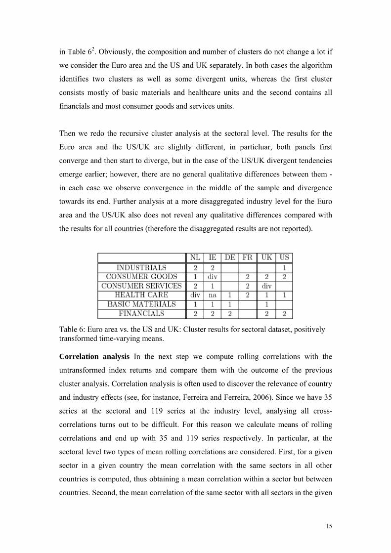
in Table 62. Obviously, the composition and number of clusters do not change a lot if

we consider the Euro area and the US and UK separately. In both cases the algorithm

identifies two clusters as well as some divergent units, whereas the first cluster

consists mostly of basic materials and healthcare units and the second contains all

financials and most consumer goods and services units.

Then we redo the recursive cluster analysis at the sectoral level. The results for the

Euro area and the US/UK are slightly different, in particluar, both panels first

converge and then start to diverge, but in the case of the US/UK divergent tendencies

emerge earlier; however, there are no general qualitative differences between them -

in each case we observe convergence in the middle of the sample and divergence

towards its end. Further analysis at a more disaggregated industry level for the Euro

area and the US/UK also does not reveal any qualitative differences compared with

the results for all countries (therefore the disaggregated results are not reported).

Table 6: Euro area vs. the US and UK: Cluster results for sectoral dataset, positively transformed time-varying means. Correlation analysis In the next step we compute rolling correlations with the

untransformed index returns and compare them with the outcome of the previous

cluster analysis. Correlation analysis is often used to discover the relevance of country

and industry effects (see, for instance, Ferreira and Ferreira, 2006). Since we have 35

series at the sectoral and 119 series at the industry level, analysing all cross-

correlations turns out to be difficult. For this reason we calculate means of rolling

correlations and end up with 35 and 119 series respectively. In particular, at the

sectoral level two types of mean rolling correlations are considered. First, for a given

sector in a given country the mean correlation with the same sectors in all other

countries is computed, thus obtaining a mean correlation within a sector but between

countries. Second, the mean correlation of the same sector with all sectors in the given

16

country is computed. This leads to mean correlations with countries but between

sectors.

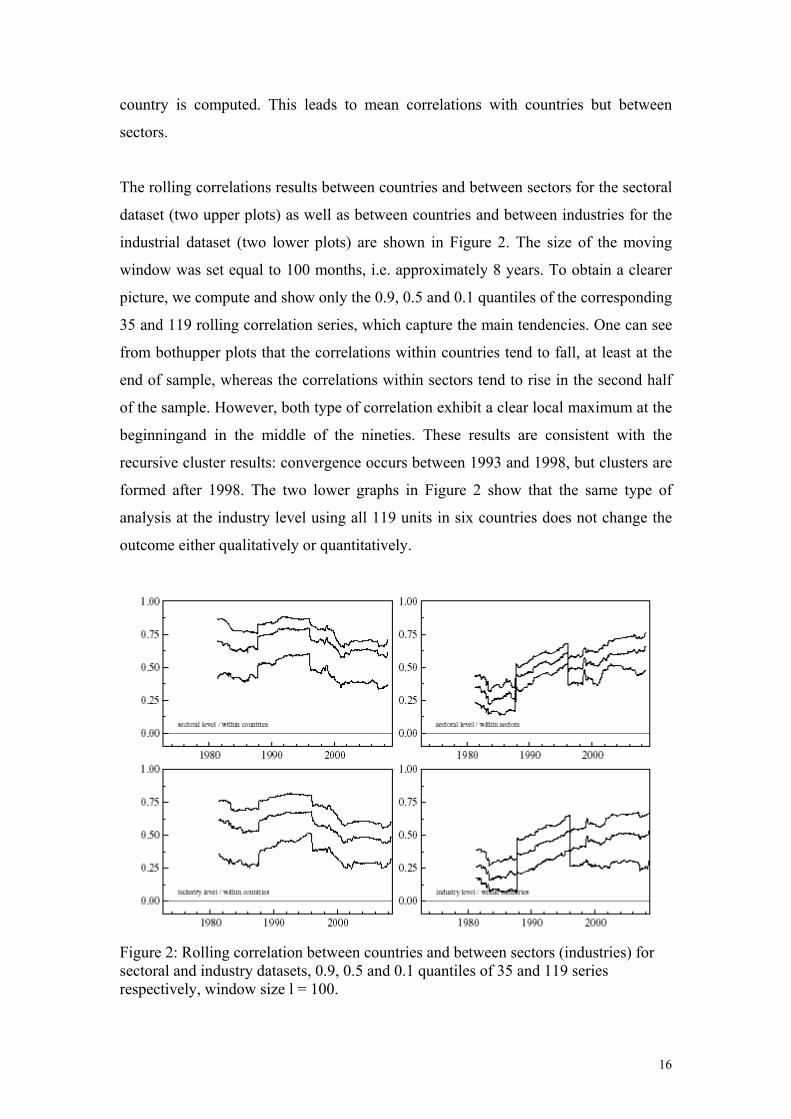
The rolling correlations results between countries and between sectors for the sectoral

dataset (two upper plots) as well as between countries and between industries for the

industrial dataset (two lower plots) are shown in Figure 2. The size of the moving

window was set equal to 100 months, i.e. approximately 8 years. To obtain a clearer

picture, we compute and show only the 0.9, 0.5 and 0.1 quantiles of the corresponding

35 and 119 rolling correlation series, which capture the main tendencies. One can see

from bothupper plots that the correlations within countries tend to fall, at least at the

end of sample, whereas the correlations within sectors tend to rise in the second half

of the sample. However, both type of correlation exhibit a clear local maximum at the

beginningand in the middle of the nineties. These results are consistent with the

recursive cluster results: convergence occurs between 1993 and 1998, but clusters are

formed after 1998. The two lower graphs in Figure 2 show that the same type of

analysis at the industry level using all 119 units in six countries does not change the

outcome either qualitatively or quantitatively.

Figure 2: Rolling correlation between countries and between sectors (industries) for sectoral and industry datasets, 0.9, 0.5 and 0.1 quantiles of 35 and 119 series respectively, window size l = 100.

17

6. Conclusions

This paper has analysed convergence in European and US financial markets using a

method recently developed by Phillips and Sul (2007) which is much more general

and flexible than alternative ones previously applied in the literature. In particular, it

is not dependent on stationarity assumptions, and is suitable for various types of

convergence processes, including clustering, which might be relevant in the case of

Europe.

European financial integration has been at the top of the EU agenda in recent years,

and has important implications for portfolio management as well. Our analysis

produces a number of interesting results. First, it shows that convergence in mean

stock returns occurred up to the late nineties, but was followed by divergence in the

subsequent period4. A plausible interpretation is that this reflects changes in the

relative importance of industry versus country effects, the latter becoming more

dominant over the years, as already reported, inter alia, by Ferreira and Ferreira

(2006). In order to investigate this issue further, we also examine cross-country and

cross-industry correlations, and find that they are both rising over time until the

nineties. However, in the following period industry correlations exhibit a positive

trend whilst country correlations tend to decline: this suggests that indeed the relative

weight of industry factors has increased, and they are behind the observed divergence

in stock returns in later years. As a result, traditional top-down investment strategies

might have to be revised; geography becomes less relevant to portfolio diversification.

This is consistent with the findings of Campa and Fernandes (2006), who study the

determinants of the evolution of country- and industry-specific returns in world

financial markets over the period from January 1973 to December 2004. They find

that the main driving force behind the significant rise in global industry shocks is the

higher integration of input and output markets in an industry, which implies a faster

transmission of shocks to the industry across countries and a higher importance of

industry factors in explaining industry returns.

4 This result is in line with those of Adjaoute and Danthine (2003), Baca et al. (2000), Cavaglia et al. (2000) and Baele et al. (2004).

18

A further question we ask is whether the policies implemented by the EU to promote

financial integration have had any noticeable effect on the observed convergence

patterns. For this purpose, we redo the analysis for subsets of countries, i.e. for the

Euro area countries in our sample, and both the UK and the US separately. The results

suggest that there are no qualitative differences between these two groups of

countries,� implying that there is a global convergence/divergence process not

obviously influenced by EU measures, but possibly driven by industry versus country

effects5. However, these results should be interpreted with caution, as our sample only

includes a small subset of EU member states (most of them, EU “core” countries), and

also the method we use focuses on medium- to long-run movements, and therefore

convergence in the short-run (highly volatile) components, especially in the case of

peripheral countries or relatively new entrants, cannot be ruled out.

Our results are highly relevant for policy makers as well. During the financial

convergence periods, policy makers should be aware that financial markets are subject

to spillover effects and a shock emerging from a certain country/industry might spread

out quickly to other countries/industries. On the other hand, divergence of equity

markets could also be an indication of a non-homogeneous financial area. In that case

policy makers should reconsider the measures to adopt to achieve a higher degree of

convergence of financial markets.

References

[1] Adam, K., Jappelli, T., Menichini, A., Padula, M., M. Pagano (2002), Analyse,

Compare, and Apply Alternative Indicators and Monitoring Methodologies to

Measure the Evolution of Capital Market Integration in the European Union, Report

to the European Commission, pages 1-95.

[2] Adjaoute, K., J. P. Danthine (2000), EMU and Portfolio Diversification

Opportunities, FAME Research Paper Series, rp31, International Center for Financial

Asset Management and Engineering.

5 Campa and Fernandes (2006) show that global industry shocks rise significantly.

19

[3] Adjaoute, K., J. P. Danthine (2003), European Financial Integration and Equity

Returns: A Theory-Based Assessment, FAME Research Paper Series, rp84,

International Center for Financial Asset Management and Engineering.

[4] Ayuso, J., R. Blanco (1999), Has Financial Market Integration Increased during

the Nineties?, Banco de Espana Working Papers, 9923.

[5] Baca, S. P., Garbe B. L., R. A. Weiss (2000), The Rise of Sector Effects in Major

Equity Markets, Financial Analysts Journal, vol. 56(5), pages 34-40.

[6] Baele, L., Ferrando, A., Hoerdahl, P., Krylova, E., C. Monnet (2004), Measuring

Financial Integration in the Euro Area, Occasional Paper Series, 14, European

Central Bank.

[7] Bai, J. (2003), Inferential Theory for Factor Models of Large Dimensions,

Econometrica, vol. 71(1), pages 135-171.

[8] Barro, R. J., X. Sala-i-Martin (1991), Convergence across States and Regions,

Brookings Papers on Economic Activity, vol. 22(1991-1), pages 107-182.

[9] Barro, R. J., X. Sala-i-Martin (1992), Convergence, The Journal of Political

Economy, vol. 100(2), pages 223-251.

[10] Bekaert, G., C. R. Harvey (1995), Time-Varying World Market Integration,

Journal of Finance, vol. 50(2), pages 403-44.

[11] Bernard, A., S. N. Durlauf (1996), Interpreting Tests of the Convergence

Hypothesis, Journal of Econometrics, vol. 71(1-2), pages 161-173.

[12] Brooks, R., M. Del Negro (2004), The Rise in Comovement Across National

Stock Markets: Market Integration or IT Bubble?, Journal of Empirical Finance, vol.

11(5), pages 659-680.

[13] Busetti, F., Fabiani, S., A. Harvey (2006), Convergence of Prices and Rates of

Infla-tion, Oxford Bulletin of Economics and Statistics, vol. 68(s1), pages 863-877.

[14] Campa, J. M., N. Fernandes (2006), Sources of Gains from International

Portfolio Diversification, Journal of Empirical Finance, vol. 13(4-5), pages 417-443.

[15] Cavaglia, S., Brightman, C., M. Aked (2000), The Increasing Importance of

Industry Factors, Financial Analysts Journal, vol. 56(5), pages 41-54.

[16] Chen, Z., P. J. Knez (1995), Measurement of Market Integration and Arbitrage,

Review of Financial Studies, vol. 8(2), pages 287-325.

[17] Durlauf, S. N., D. T. Quah (1999), The New Empirics of Economic Growth, in:

Taylor J. B., M. Woodford (ed.), Handbook of Macroeconomics, edition 1, volume 1,

chapter 4, pages 235-308.

20

[18] Ferreira M. A., P. M. Gama (2005), Have World, Country and Industry Risk

Changed Over Time? An Investigation of the Developed Stock Markets Volatility,

Journal of Financial and Quantitative Analysis, vol. 40(1), pages 195-222.

[19] Ferreira M. A., M. A. Ferreira (2006), The Importance of Industry and Country

Effects in the EMU Equity Markets, European Financial Management, vol. 12(3),

pages 341-373.

[20] Fratzscher, M. (2002), Financial Market Integration in Europe: On the Effects of

EMU on Stock Markets, International Journal of Finance and Economics, vol. 7(3),

pages 165-93.

[21] Fritsche, U., V. Kuzin (2008), Analysing Convergence in Europe Using a Non-

linear Single Factor Model, Macroeconomics and Finance Series, 200802, Hamburg

University, Department Wirtschaft und Politik.

[22] Goetzmann, W. N., Lingfeng L., K. G. Rouwenhorst (2005), Long-Term Global

Market Correlations, Journal of Business, vol. 78(1), pages 1-38.

[23] Hardouvelis, G. A., Malliaropulos, D., R. Priestley (2007), The Impact of EMU

on the Equity Cost of Capital, Journal of International Money and Finance, vol.

26(2), pages 305-327.

[24] Heston, S., K. G. Rouwenhorst (1994), Does Industrial Structure Explain the

Benefits of International Diversification?, Journal of Financial Economics, vol. 36(1),

pages 3-27.

[25] Hobijn, B., P. H. Franses (2000), Asymptotically Perfect and Relative

Convergence of Productivity, Journal of Applied Econometrics, vol. 15(1), pages 59-

81.

[26] Islam, N. (2003), What have We Learnt from the Convergence Debate?, Journal

of Economic Surveys, vol. 17(3), pages 309-362.

[27] Lessard, D. R. (1973), World, National, and Industry Factors in Equity Returns,

Journal of Finance, vol. 29(2), pages 379-391, Papers and Proceedings of the Thirty-

Second Annual Meeting of the American Finance Association.

[28] Phillips, P.C., D. Sul (2007), Transition Modeling and Econometric Convergence

Tests, Econometrica, vol. 75(6), pages 1771-1855.

[29] Stock, H.J., M. W. Watson (1998), Median Unbiased Estimation of Coefficient

Variance in a Time-Varying Parameter Model, Journal of the American Statistical

Association, vol. 93(441), pages 349-358.

21

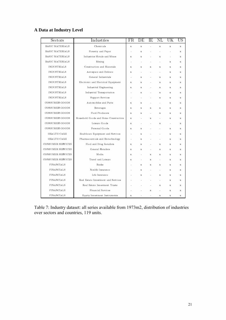
A Data at Industry Level

Table 7: Industry dataset: all series available from 1973m2, distribution of industries over sectors and countries, 119 units.