TEST GRIDS FOR RELIABILITY ANALYSIS

Analysing interruptions and developing test grids based on Mälarenergi Elnät distribution grid

JONAS ELD

JENS MELIN

School of Business, Society and Engineering Energy Engineering Degree Project 30 hp Master program in engineering, Energy System ERA403

Supervisor: Jan Sandberg Examiner: Maher Azaza Customer: Stefan Svensson, Mälarenergi Elnät AB Date: 2017-06-08 Email: jed12004@student.mdh.se jmn12008@student.mdh.se

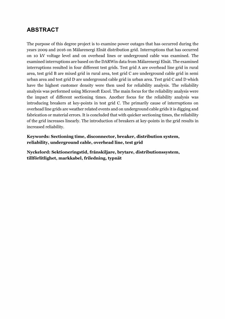
ABSTRACT

The purpose of this degree project is to examine power outages that has occurred during the

years 2009 and 2016 on Mälarenergi Elnät distribution grid. Interruptions that has occurred

on 10 kV voltage level and on overhead lines or underground cable was examined. The

examined interruptions are based on the DARWin data from Mälarenergi Elnät. The examined

interruptions resulted in four different test grids. Test grid A are overhead line grid in rural

area, test grid B are mixed grid in rural area, test grid C are underground cable grid in semi

urban area and test grid D are underground cable grid in urban area. Test grid C and D which

have the highest customer density were then used for reliability analysis. The reliability

analysis was performed using Microsoft Excel. The main focus for the reliability analysis were

the impact of different sectioning times. Another focus for the reliability analysis was

introducing breakers at key-points in test grid C. The primarily cause of interruptions on

overhead line grids are weather related events and on underground cable grids it is digging and

fabrication or material errors. It is concluded that with quicker sectioning times, the reliability

of the grid increases linearly. The introduction of breakers at key-points in the grid results in

increased reliability.

Keywords: Sectioning time, disconnector, breaker, distribution system,

reliability, underground cable, overhead line, test grid

Nyckelord: Sektioneringstid, frånskiljare, brytare, distributionssystem,

tillförlitlighet, markkabel, friledning, typnät

PREFACE

This degree project in Master of Science energy system have been carried out at Mälarenergi

Elnät AB. We would like to thank the people at Mälarenergi Elnät AB who has helped us with

the project. Special thanks to our supervisor Stefan Svensson for providing support and

technical knowledge throughout the degree project. We would also like to thank Johanna

Rosenlind for the support throughout the project. Also special thanks to Marcus Nilsson for

his expertise regarding the operations of the grid.

We would furthermore like to thank our supervisor Jan Sandberg at Mälardalen University

who has contributed throughout this degree project.

Västerås in June 2017

Jonas Eld & Jens Melin

…………………………….… …………………………….…

SUMMARY

Power distribution with a high reliability is necessary for the modern society. The distribution

grid plays a fundamental role in order to supply reliable electricity to the consumers.

Interruptions in the delivery of electricity comes with a high societal cost. Different sectors and

customers have different costs for an interruption.

The purpose of this degree project were to examine the interruptions that have occurred on the

voltage level of 10 kV affecting the overhead lines and underground cables within the

Mälarenergi Elnät distribution grid. From the examined interruptions different test grids were

developed. Further aspects that was considered were the cause of the outage and what day they

occurred on.

DARWin data for the years 2009 to 2016 was used to conduct the degree project. The software

Trimble NIS was used to examine the grid and collect the information of the cable types,

substations, customers and the structure of the grid. Based on the data collected from DARWin

and Trimble different test grids were created with different criteria’s. The criteria’s for the

construction of the test grids were the amount of underground cable compared to the amount

of overhead line and as sub criteria the customer density was used.

The test grids with the highest customer density was then used for reliability analysis. The cost

for an interruption on these test grids was also calculated, based on the customer composition

on these grids. Since the grids were structured as loops with multiple possible back-up feeds,

different sectioning times were used to examine how the reliability indicators varied with

shorter or longer sectioning times.

One additional scenario was also considered. This scenario consisted of installing breakers at

key-points in the grid. For the base scenarios, breakers were only installed in the primary

substation.

The examined components in the distribution grid, overhead line and underground cable, have

the most number of interruptions. The cause of the interruptions are on overhead line mainly

weather related and for underground cable it is digging and fabrications or material failures

that are the most common causes. The spread on the numbers of interruptions during the week

are quite even, except for the underground cable which has a clear drop during the weekends.

The reason for the drop are that the interruptions that is caused by digging is not as frequent

during the weekends. It is concluded that the interruption cost changes linearly with the

sectioning time. Installing breakers at key-points in the grid increases the reliability.

SAMMANFATTNING

Eldistribution med en hög tillförlitlighet är en viktig aspekt för det moderna samhället.

Kostnaderna för samhället vid strömavbrott är höga och olika sektorer samt kunder har olika

kostnader vid ett eventuellt avbrott. Distributionsnätet spelar en stor roll i tillförlitligheten för

distributionen av elektricitet.

Syftet med detta examensarbete är att undersöka de avbrott som har skett på 10 kV’s

friledningar och markkablar inom Mälarenergi Elnäts distributionsnät. Sedan skapades typnät

utifrån de mest drabbade nätsektionerna. Vidare så undersöktes också orsaken till avbrotten

även vilken dag i veckan avbrotten inträffade.

DARWin data från åren 2009 till och med 2016 användes som grund för detta arbete.

Programmet TRIMBLE NIS användes för att studera strukturen på distributionsnätet och för

att sammanställa data om markkablar, friledningar, nätstationer och kunder. Typnäten som

sedan konstruerades baserades på denna data. Typnäten delades in beroende på andelen

markkabel och kundtätheten.

De typnäten med störst kundtäthet användes sedan för att genomföra tillförlighetsanalyser.

Kundkostnaderna för ett eventuellt avbrott beräknades också för dessa typnät. Typnäten var

uppbyggda som slingade nät med flera möjliga omkopplingar. Detta gjorde att

sektioneringstiden för dessa omkopplingar användes som variabel för tillförlighetsanalysen.

Ytterligare ett beräkningsscenario genomfördes. Detta scenario byggde på att installera extra

brytare i vissa viktiga punkter i nätet. Som standard var endast mottagningsstationerna

installerade med brytare.

De studerade komponenterna, friledning och markkabel, är de komponenterna i

distributionsnätet som har flest avbrott. De vanligaste orsakerna för dessa avbrott är

väderrelaterade på friledningar och avgrävning samt fabrikationsfel på markkablar. Avbrotten

är jämt fördelade över veckan, förutom för markkablar där antalet avbrott minskar tydligt på

helger. Anledningen till denna minskning på helger är att antalet grävningar och då också

antalet avgrävningar minskar. Avbrottskostnaderna ändrades linjärt med sektioneringstiden.

Att installera brytare in i viktiga punkter i nätet höjde tillförlitligheten.

TABLE OF CONTENT

1 INTRODUCTION .............................................................................................................1

1.1 Background ............................................................................................................. 1

1.1.1 Mälarenergi Elnät AB ....................................................................................... 2

1.1.2 Previous research ............................................................................................ 2

1.2 Problem formulation................................................................................................ 3

1.3 Purpose of degree project ...................................................................................... 3

1.4 Research questions ................................................................................................ 4

1.5 Delimitation .............................................................................................................. 4

2 METHOD .........................................................................................................................5

2.1 The literature review ................................................................................................ 5

2.2 The empirical research ............................................................................................ 5

3 THE SWEDISH ELECTRICITY GRID ..............................................................................6

3.1 Grid structure .......................................................................................................... 6

3.2 The Swedish electricity market reform 1996 ......................................................... 8

3.2.1 Reliability of delivery ........................................................................................ 9

3.2.2 The impact of Gudrun ...................................................................................... 9

3.2.3 DARWin ..........................................................................................................10

3.2.4 Interruption cost ..............................................................................................12

3.3 Overhead line and underground cable..................................................................13

3.3.1 Overhead line .................................................................................................13

3.3.2 Underground cable .........................................................................................15

3.4 Control system .......................................................................................................17

4 DISTRIBUTION SYSTEM RELIABILITY ....................................................................... 19

4.1 DARWin-file .............................................................................................................19

4.1.1 Overhead line .................................................................................................19

4.1.2 Underground cable .........................................................................................19

4.1.3 Evaluation of DARWin-file ...............................................................................20

4.2 Modelling of test grids ...........................................................................................20

4.2.1 Data collection ................................................................................................20

4.2.2 Classification of the test grids ..........................................................................20

4.2.3 Description of the structure of the test grids ....................................................21

4.2.4 Specifications of the different test grids ...........................................................22

4.3 Analytical reliability analysis .................................................................................26

4.3.1 Failure rate ......................................................................................................26

4.3.2 Unavailability ...................................................................................................27

4.3.3 Reliability indicators ........................................................................................27

4.3.4 Base scenario .................................................................................................28

4.3.5 Different sectioning times ................................................................................28

4.3.6 Design suggestion for Test grid C ...................................................................28

4.3.7 Calculations ....................................................................................................29

5 RESULTS ...................................................................................................................... 31

5.1 Histograms of the interruptions ............................................................................31

5.2 Test grid A ...............................................................................................................33

5.3 Test grid B ...............................................................................................................34

5.4 Test grid C ...............................................................................................................35

5.5 Test grid D ...............................................................................................................37

5.6 Design suggestion for test grid C .........................................................................39

5.7 Sensitivity analysis ................................................................................................40

6 DISCUSSION................................................................................................................. 43

6.1 Empirical research .................................................................................................43

6.2 Result ......................................................................................................................43

7 CONCLUSIONS ............................................................................................................ 45

8 FUTURE WORK ............................................................................................................ 45

REFERENCES ..................................................................................................................... 46

APPENDIX 1 – CABLE DESIGNATION STANDARDS

APPENDIX 2 – TEST GRID A

APPENDIX 3 – TEST GRID B

APPENDIX 4 – TEST GRID C

APPENDIX 5 – TEST GRID D

APPENDIX 6 – DESIGN SUGGESTION TEST GRID C

APPENDIX 7 – DESCRIPTIONS OF CALCULATIONS

LIST OF FIGURES

Figure 1: Double cable structure. ............................................................................................... 7

Figure 2: Loop structure. ........................................................................................................... 7

Figure 3: Radial structure. ......................................................................................................... 8

Figure 4: Free overhead line (isolated and uninsulated) in use at the voltage level of 10 kV...14

Figure 5: Line street overhead line. .......................................................................................... 15

Figure 6: Underground cable types in use at the voltage level of 10kV in the MEE grid. ........16

Figure 7: Schematic over Test grid A. ...................................................................................... 23

Figure 8: Schematic over Test grid B. ...................................................................................... 23

Figure 9: Schematic over Test grid C. ...................................................................................... 24

Figure 10: Schematic over Test grid D. .................................................................................... 24

Figure 11: Schematic over the design suggestion for Test grid C. ............................................ 29

Figure 12: Interruptions on components at the voltage level of 10 kV during the years 2009-

2016. .......................................................................................................................................... 31

Figure 13: Interruption causes on overhead line and underground cable 10 kV 2009-2016. . 32

Figure 14: Number of interruptions per day at the voltage level of 10 kV and on overhead line

and underground cable during the years 2009-2016. ............................................................. 32

Figure 15: Interruptions on overhead line sorted by day. ........................................................ 33

Figure 16: Interruptions on underground cable sorted by day. ............................................... 33

Figure 17: Interruptions by category on Test grid A. ............................................................... 34

Figure 18: Interruptions by cause on Test grid A. .................................................................... 34

Figure 19: Interruptions by category on Test grid B. ............................................................... 35

Figure 20: Interruptions by cause on Test grid B. ................................................................... 35

Figure 21: Interruption by category on Test grid C. ................................................................. 36

Figure 22: Interruptions by cause on Test grid C. ................................................................... 36

Figure 23: Interruption costs Test grid C. ................................................................................ 37

Figure 24: Interruptions by category on Test grid D. .............................................................. 38

Figure 25: Interruptions by cause on Test grid D. ................................................................... 38

Figure 26: Interruption costs Test grid D. ............................................................................... 39

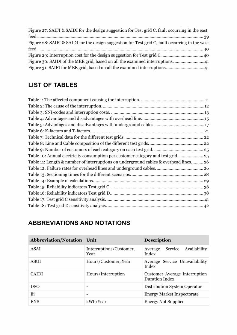
Figure 27: SAIFI & SAIDI for the design suggestion for Test grid C, fault occurring in the east

feed. .......................................................................................................................................... 39

Figure 28: SAIFI & SAIDI for the design suggestion for Test grid C, fault occurring in the west

feed. .......................................................................................................................................... 40

Figure 29: Interruption cost for the design suggestion for Test grid C. .................................. 40

Figure 30: SAIDI of the MEE grid, based on all the examined interruptions. .........................41

Figure 31: SAIFI for MEE grid, based on all the examined interruptions. ...............................41

LIST OF TABLES

Table 1: The affected component causing the interruption. ..................................................... 11

Table 2: The cause of the interruption. .....................................................................................12

Table 3: SNI-codes and interruption costs. .............................................................................. 13

Table 4: Advantages and disadvantages with overhead line. .................................................... 15

Table 5: Advantages and disadvantages with underground cables. ......................................... 17

Table 6: K-factors and T-factors. ..............................................................................................21

Table 7: Technical data for the different test grids. ................................................................. 22

Table 8: Line and Cable composition of the different test grids. ............................................. 22

Table 9: Number of customers of each category on each test grid. ......................................... 25

Table 10: Annual electricity consumption per customer category and test grid. .................... 25

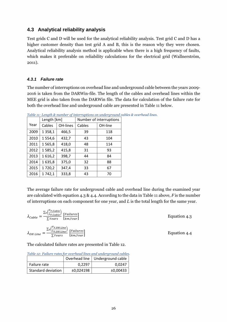
Table 11: Length & number of interruptions on underground cables & overhead lines. ......... 26

Table 12: Failure rates for overhead lines and underground cables. ....................................... 26

Table 13: Sectioning times for the different scenarios. ............................................................ 28

Table 14: Example of calculations. ........................................................................................... 29

Table 15: Reliability indicators Test grid C. ............................................................................. 36

Table 16: Reliability indicators Test grid D. ............................................................................. 38

Table 17: Test grid C sensitivity analysis. ..................................................................................41

Table 18: Test grid D sensitivity analysis. ................................................................................ 42

ABBREVIATIONS AND NOTATIONS

Abbreviation/Notation Unit Description

ASAI Interruptions/Customer, Year

Average Service Availability Index

ASUI Hours/Customer, Year Average Service Unavailability Index

CAIDI Hours/Interruption Customer Average Interruption Duration Index

DSO - Distribution System Operator

Ei - Energy Market Inspectorate

ENS kWh/Year Energy Not Supplied

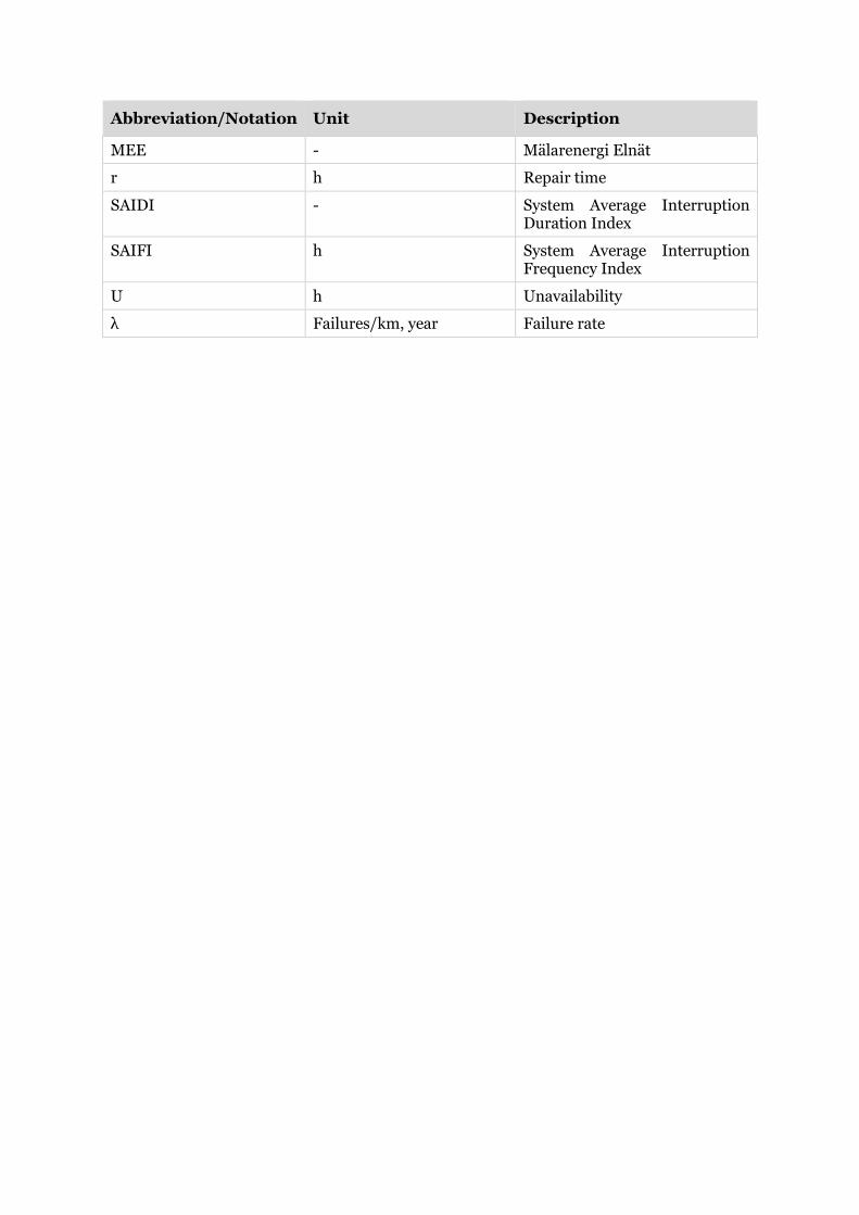
Abbreviation/Notation Unit Description

MEE - Mälarenergi Elnät

r h Repair time

SAIDI - System Average Interruption Duration Index

SAIFI h System Average Interruption Frequency Index

U h Unavailability

λ Failures/km, year Failure rate

1

1 INTRODUCTION

Power distribution with a high availability is necessary for the modern society and the future

development of the modern world. (Wallnerström & Grahn, 2016)

In order to supply reliable electricity to the consumer, the power distribution grid plays a

fundamental role (Cadini, et al., 2017). The baseline of this degree project is to examine the

current most affected overhead line and underground cable grids, at 10 kV, and by different

criteria construct them into several test grids. Then, the test grids could be used for analytical

reliability analysis.

1.1 Background

Power outages generates a high societal cost. In the case of an outage, all the different parts of

the society is affected. Sectors and customers are affected differently; some industries and

services are affected independently of the length of the outage, and some are more affected by

longer outages. Hospitals and other crucial public services often have backup generators, but

the vulnerability of operation is significantly increased following power outages.

(Wallnerström & Grahn, 2016)

The electricity act (SFS 1997:857) specifies that the transfer of electricity should be of good

quality (3rd Chapter, 9§)

The Energy market inspectorate (Ei) in Sweden also specifies the requirements for power

distribution quality. Those requirements include for instance, the maximum number of power

outages per year, and voltage quality, among others. The Distribution System Operator (DSO)

is responsible for the distribution grid in their area. (Morén, 2013)

Each year, the DSOs is responsible for submitting information about the power outages in their

grid to Ei, through a system called DARWin. DARWin is a statistical database that makes it

possible for the DSOs and Ei to steer investments and maintenance to those parts in the grid

where the investments are needed mostly. (Wallnerström & Grahn, 2016)

The distribution grid is a local monopoly and therefore there is a need for some control on how

much the customer will have to pay to the DSO to be connected to the grid. In the year 2009

the government in Sweden decided to change the electricity act (SFS 1997:857) so that the grid

tariffs’ fairness should be examined beforehand in a so called ex-ante regulation. This

regulation means that Ei in advance, decides the allowed revenue for each DSO depending on

the reliability of the grid. (Ström, 2015)

2

The reason for this regulation is to counteract the potential risk of decreasing quality due to

the monopoly situation for the DSOs. There is a risk that the reliability is decreasing in the grid

in order to maximize the profit for the DSOs. (Ström, 2015)

To steer towards increased grid reliability cost effectively it is helpful to construct test grids,

which can be a normalization of the actual grid for the current DSO. Using these test grids, it

is possible to calculate the effects of different improvement efforts before implementing the

new changes (Engblom & Ueda, 2007). One way to measure and compare the effects of power

outages is to calculate the SAIFI and SAIDI for each outage. SAIFI is the number of customers

affected and SAIDI is how long each customer is affected by the power outage.

The more precise the test grids can be, the more helpful they are for the DSO. In this degree

project, different test grids are constructed based on the current grid at MEE. The DARWin

report from the DSO Mälarenergi Elnät AB is used to search for certain areas in the grid where

power outages are more or less clustered and moreover if there are any distinct similarities or

differences between these areas.

1.1.1 Mälarenergi Elnät AB

Mälarenergi Elnät AB is the DSO for the grid in the municipalities of Arboga, Hallstahammar,

Kungsör, Köping and Västerås. The grid stretches over the western part of Mälardalen. MEE

distributes electricity to over 100 000 customers through the local distribution grid. As the

DSO for this area, MEE is responsible for operation and maintenance of the distribution grid.

According to the regulations stated by Ei, MEE is accountable for the quality of distribution.

(Mälarenergi AB, 2015)

1.1.2 Previous research

Previous work has been done when constructing test grids that is representative for Sweden as

a whole. The purpose of that project was to construct different test grids for the countryside

and urban areas. These grids were used for reliability and interruption cost calculations.

(Engblom & Ueda, 2007)

Other studies have created reliability test systems for learning purposes, based on statistics

from other studies and then combined into a test system. The test system contains all the

components found in a real system but it is small enough for students and others to perform

calculations by hand. (Allan, et al., 1991)

The test system constructed by (Ueda, et al., 2009) describes the Swedish distribution grid as

two different type grids, one rural and one urban. This is a simplification of Swedish grid.

All these test systems have been created to fit many different grids due to an underlying

purpose of generalisation. In this degree project test grids are constructed with the specific grid

at MEE as a base system, due to a purpose of specificity.

3

1.2 Problem formulation

Overhead lines are often replaced with underground cables to get rid of weather-related power

outages. Decreasing outages has a direct correlation to increased grid reliability. There are

disadvantages with underground cables, compared to overhead lines. Underground cables are

2 – 10 times more expensive than overhead line and it is harder to localize faults along the

length of the cable (Svensson, 2012).

Replacing overhead line with underground cable is a measure to decrease the number of

outages. For the duration of an outage, the sectioning time is of importance. The sectioning

time is the time it takes to isolate the fault and reconnect the customers. Longer sectioning

time leads to an increased cost. The sectioning is mainly done manually by fitters on sight. The

sectioning time often depends on the experience of the operators and fitters.

There will be both overhead lines and underground cables in the future electricity grid, hence

creating test grids comprising both of them is of significant importance.

The most important aspect of using test grids, involves and understanding on how to tailor the

model to suit the particular needs of the MEE grid. Previously-developed test grids could be

considered too general and the underlying assumptions could be too restrictive, prohibiting a

valuable analysis. In reality, the grid is a complex entity and looks different depending on

aspects such as: amount of underground cables, overhead lines, rural and urban areas and the

geographical location. All of this points to the fact that a tailored test grid, representable for

the MEE grid, should be considered superior when it comes down to examining and analysing

the grid reliability.

1.3 Purpose of degree project

The purpose of this degree project is to examine the power outages that has occurred on

overhead lines and underground cables at the voltage level of 10 kV within the MEE grid.

Further aspects that will be considered are: the cause of the power outages and the day of the

outages. This degree project will be performed by using test grids constructed by relevant

criteria with a relevant connection to the MEE grid. Then, the test grids are used for an

investigation of the different types of outages and their corresponding consequence. The

outcome of the analysis will be the interruption costs that occurs in the event of an

interruption.

4

1.4 Research questions

The research questions in this degree project are stated in the following bulleted list.

What impact have the day of the week on the number of interruptions?

What causes the interruptions that occurs in the different grid sections?

How does the sectioning time affect the interruption cost in semi urban and urban grids?

How does more breakers in the grid influence the reliability?

1.5 Delimitation

The examined power outages in this degree project are the ones that occurs on underground

cables and overhead lines. These two components are seen as the major criteria’s when creating

test grids. The examined interruptions are spread throughout the MEE concession area. The

voltage level examined is 10 kV. Planned outages are not considered in this degree project. The

outage data that is examined originated from events occurring during the years 2009-2016,

but the grid could, in some, locations be altered with new equipment and/or changes from

overhead lines to underground cable could have occurred, for example. This factor has not

been taken into consideration, and the grid “as is” right now is assumed to be the same as 2009.

For the reliability and cost calculations, only one interruption at a time will be considered. The

reliability and cost calculations will be performed on the test grids with the highest customer

density.

5

2 METHOD

The method to achieve the objectives in this degree project is divided in to two parts: literature

reviewing and empirical researching.

2.1 The literature review

A literature study was carried out by reading articles journals, books and degree projects within

the subject. Electrical power distribution systems were examined. Theories about reliability

was also examined. The Swedish electricity markets rules and regulations were examined. The

article journals have been found on different databases through the university library at

Mälardalen högskola. The construction of overhead lines and underground cables have been

examined and is described in chapter 3. Construction of test grids has been examined from

different articles and discussed with the supervisor at MEE.

2.2 The empirical research

The empirical research includes collecting information through discussions with employees at

MEE and gathering data from historical records on power outages. The research is mainly on

gathering data from historical records on power outages inside MEE concession area. Data

comes from the database DARWin (managed by Energiföretagen Sverige). The empirical

research include collecting information from discussions. The discussions have been

performed with employees at MEE with extensive experience and technical knowledge on the

electricity grid, within their own concession area.

In order to examine the structure of the grid along with geography, the software Trimble NIS

is used. Using this software, the grid structure and different parts of the system could be

examined. The geography of the area surrounding the grid could also be analysed in this

software.

The ten most affected grid sections were examined and classified into different grid types

(overhead line, underground cable or mixed) and customer density. For each grid section,

certain data was collected.

The data collected during the empirical research were used for modelling the test grids and for

reliability calculations. The analytical reliability analysis was conducted using Microsoft Excel.

6

3 THE SWEDISH ELECTRICITY GRID

The Swedish electricity grid is divided into three different levels depending on the voltage, the

national grid, regional grid and the local grid (also called the distribution grid). The national

grid is the backbone of the electricity grid in Sweden (Pettersson, 2017). It transfers the

electricity from the large hydro power plants in the northern part of Sweden, to the south where

most of the consumers are accommodated. The nuclear power plants are also connected to the

national grid (Wallnerström & Grahn, 2016). The voltage in the national grid is 220kV or

400kV, the reason for the high voltage is to minimize the losses when transferring the power

over long distances (Konsumenternas Energimarknadsbyrå, 2017).

The national grid is connected to the regional grid, where the voltage is between 40kV to 130kV

(Konsumenternas Energimarknadsbyrå, 2017). Wind power plants and other smaller power

plants are connected to the regional grid. The regional grid transfers the power from the

national grid and the power plants directly connected to the regional grid to the local grid and

also to the customers directly connected to the regional grid (Konsumenternas

Energimarknadsbyrå, 2017; Wallnerström & Grahn, 2016).

The last level is the local grid (or the distribution grid), this is where most of the customers are

connected. The distribution grid is divided into two different voltage levels, 10kV and 0,4kV.

Industries and other high consuming customers are connected to the 10kV grid. The

distribution grid is constructed in different ways depending on the density of the customers

and the need for redundancy (Söder & Amelin, 2011).

3.1 Grid structure

The structure of the distribution grid is mainly dependent on economic aspects. Constructing

redundant distribution grids is not economically viable in all places. In Sweden, the

distribution grid is mainly structured in one of the three following ways (Engblom & Ueda,

2007).

Double cable structure

Loop structure

Radial structure

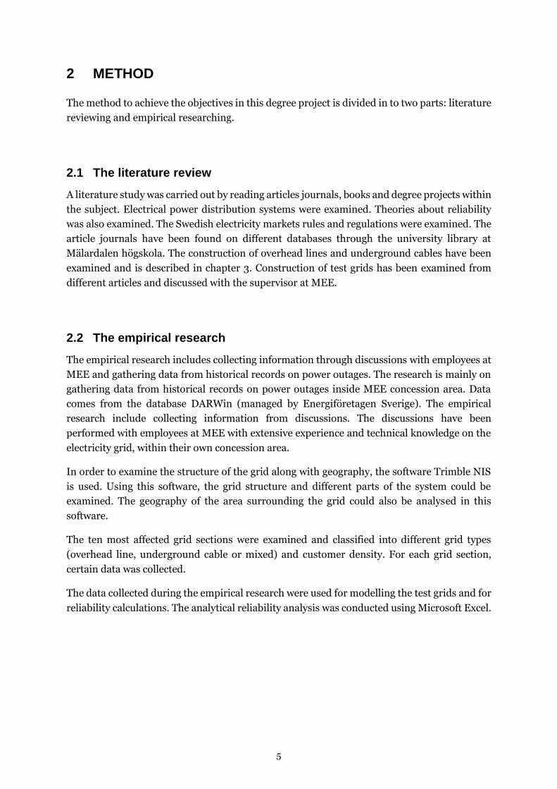
Normally, these three structures are used and combined into a single grid entity. Double cable

structure is used in the city center where a high reliability level is required and economically

viable. In this structure, each substation is connected to two parallel cables. This structure has

a fast reconnection in case of a power outage, the reconnection from the faulty component is

done automatically and therefore the average outage time is less than 1 minute (Engblom &

Ueda, 2007). An illustration of a double cable structure is presented in Figure 1 below.

7

Figure 1: Double cable structure.

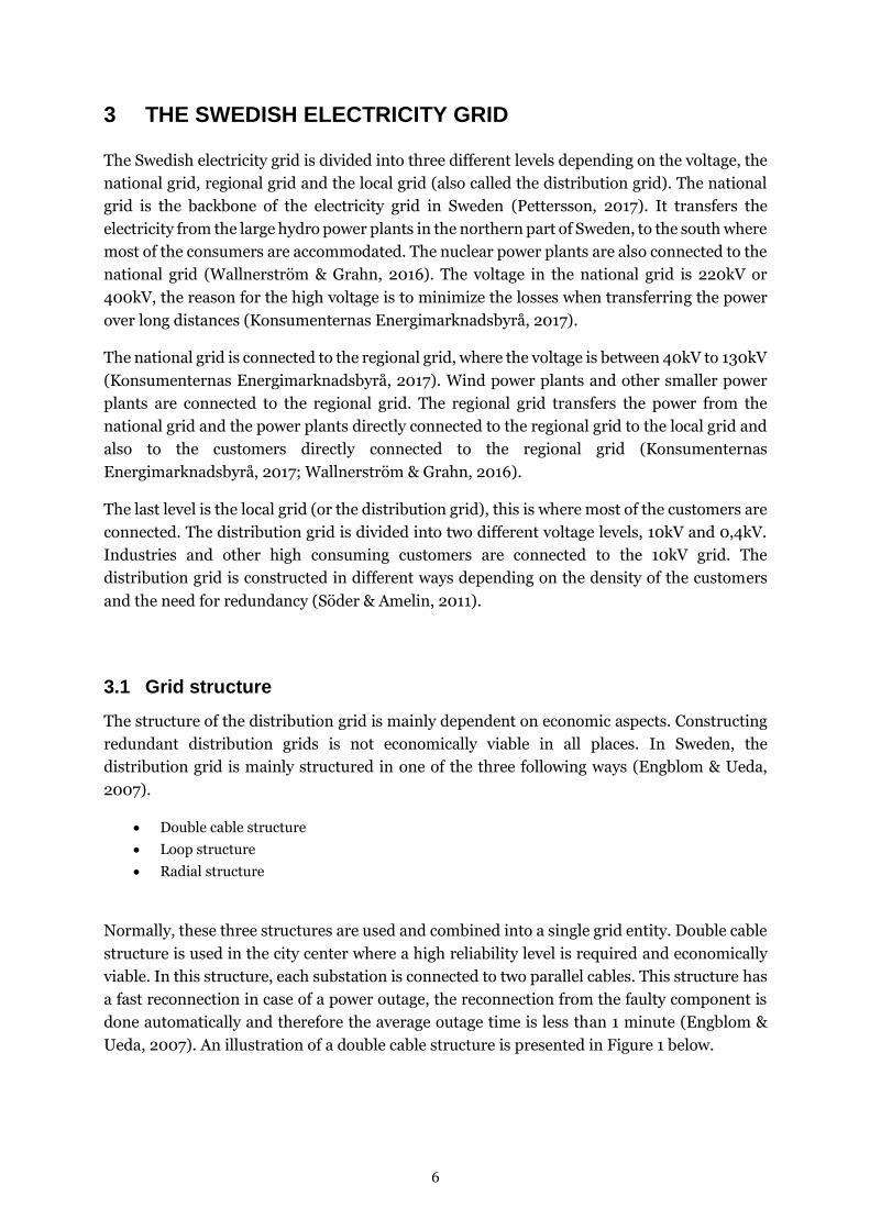
The looped structure is the most common way of structuring a distribution grid. The

characteristic of a looped structure is that each substation has the possibility to be feed from a

different primary substation (Engblom & Ueda, 2007). The looped grid is almost always run

as a radial grid, which means that the loop is split into two radial sections by a disconnector,

fed from two different slots from a primary substation. Sometimes the grid is fed from two

different primary substations (Lexholm, 2016).

The breakers in the primary substation will, in case of a fault, disconnect all the substations

fed from that slot. Before the customers can be reconnected, by closing the disconnector that

splits the loop, the fault location needs to be found and this is often done by personnel on site

(Lexholm, 2016). Also, the reconnection is done manually, this leads to an average down time

equal to 0,5 to 2,5 hours (Engblom & Ueda, 2007). In Figure 2 below, an illustration of a looped

structure is presented.

Figure 2: Loop structure.

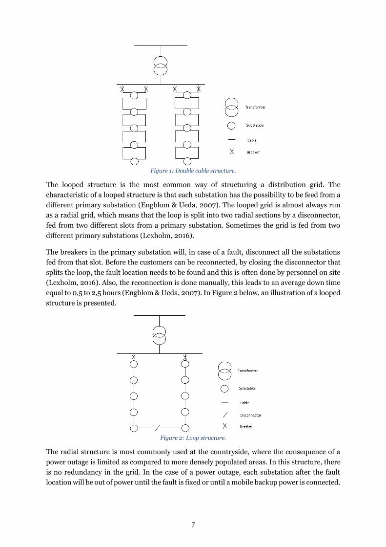
The radial structure is most commonly used at the countryside, where the consequence of a

power outage is limited as compared to more densely populated areas. In this structure, there

is no redundancy in the grid. In the case of a power outage, each substation after the fault

location will be out of power until the fault is fixed or until a mobile backup power is connected.

8

The average down time for a radial grid is approximately between 1 and 12 hours (Engblom &

Ueda, 2007).

In a radial containing overhead lines, there is often an installed delayed reconnection on the

breaker in the primary substation slot. In case of a transient fault, the customers will have their

power back after a short period without any work done by personnel (Lexholm, 2016).

Transient errors on overhead lines is often caused by tree branches touching the lines or

lightning strikes (Torstensson & Bollen, 2012). An illustration of a radial structure is presented

in Figure 3 below.

Figure 3: Radial structure.

3.2 The Swedish electricity market reform 1996

The electricity market was at the beginning a monopoly business, the DSOs was given an

obligation to deliver electricity to its customers inside their concession area. Then, the DSOs

had a sort of monopoly position of selling electricity to the connected customers (Banefelt &

Larsson, 2006).

To make the electricity market more rational and effective, a new electricity market reform was

made in 1996 (Banefelt & Larsson, 2006). In this reform, it is stated that production or selling

of electricity cannot be conducted by a legal person that is also the concession owner (SFS

1997:857). The reform implies that the DSOs only have an obligation to distribute the

electricity and not deliver to its connected customers. This allows the customer to choose where

to buy their electricity. The purpose of the reform was to make the electricity market more

competitive and to get rid of the monopoly business. Distribution of electricity is still

conducted on a monopoly market, but the monitoring and control is done by a new authority

(Banefelt & Larsson, 2006).

The supervision of the grid operations is done by the so called “Network authority”. The tasks

of the network authority is in the hands of the Energy Market Inspectorate (Ei). There are two

parts that the Ei is not in charge of, the safety of the grid - which is in the hands of the

9

“Elsäkerhetsverket”, and the competitive part (production and trade) – which is in the hands

of the Swedish Competition Authority (Banefelt & Larsson, 2006).

3.2.1 Reliability of delivery

The electricity act (SFS 1997:857) specifies that the transfer of electricity should be of good

quality (3rd Chapter, 9§). Quality, in this case, involves delivery reliability and voltage quality.

The reliability of the delivery means the probability that the power will be distributed to the

customer. The voltage quality of the delivery implies that the power can be distributed to the

customer without disruption in the voltage (excluding power outages).

The distribution to low-voltage consumers, such as household, the delivery is of good quality

if there are no more than three unannounced outages that exceeds three minutes per year. If

the number of unannounced outages exceeds eleven per year, the quality is not of good quality

(Morén, 2013).

The general voltage quality regulations are specified in the EIFS 2013:1 7th chapter (Morén,

2013).

The distribution companies have incentives for maintaining a good quality of the distribution

provided by the Ei. These incentives were introduced in order to motivate the distribution

companies to, on their own, increase the reliability of delivery and to make investments and

conduct maintenance on the electricity grid, according to best practice. The delivery reliability

affects the income frame for the company, increasing the reliability of the grid can lead to a

bigger income frame for the company and vice versa (Wallnerström & Grahn, 2016).

3.2.2 The impact of Gudrun

In 2005, the southern part of Sweden was hit by the storm Gudrun. The storm gave rise to a

numerous amount of outages that, not only affected the electricity grid, but also the railway

network, telecommunication network and the mobile communication network (Banefelt &

Larsson, 2006). For the electricity grid, the local grid was affected the most but the regional

grid was also affected (Heden & Johansson, 2005). The impact of the storm was enormous, it

left people power less for days, and for some, even weeks (Energimyndigheten, 2015). The

direct costs for the DSOs, as a result of the storm, were also extremely high, the highest cost

affected the DSO Sydkraft that had an estimated cost of 1 690 000 000 SEK (Heden &

Johansson, 2005).

Gudrun was a tipping point when it comes to reliable electricity distribution, after the storm

the Swedish government gave a mission to the Ei. The mission was to leave suggestions on how

the reliability for the power distribution can be obtained, and regulations that keeps the grid

companies to follow these suggestions (Banefelt & Larsson, 2006). The Ei came up with

suggestions that could be added into the already consisted electricity act. Two of the

suggestions that was added to the electricity act were (Engblom & Ueda, 2007):

10

The duration of an outage should not exceed 24 hours.

If the duration of an outage lasts between 12 and 24 hours, the DSO will pay a fee of 12,5

% of the costumers calculated yearly grid fee.

The compensation fee, mentioned above, for outages longer than 12 hours is a percentage of

the yearly cost for the grid for the customer but no less than 900kr and it increases for every

24-hour period to a maximum of 300 percent of the annual cost for the customer (Engblom &

Ueda, 2007).

It further states that the DSOs should every year conduct a risk and vulnerability analysis of its

electrical distribution, as another suggestion of the Ei (Banefelt & Larsson, 2006). This will

allow the DSOs to have an overview of the electrical distribution system and to see where

investment could be allocated to achieve an increased reliability level. The Ei also announced

that it will impose on the DSOs to report any outages that has a duration of 3 minutes or higher.

3.2.3 DARWin

During the years 1988 – 1990 a system for interruption and outage reporting was developed

that was called DAR. DAR was used by approximately 40 DSOs, DAR was an upgrade from the

previous system FAR-81. The new electricity reform in 1996 lead to higher demand for

interruption and outage reporting (Jansson, 2000). This followed that the DAR system was

upgraded to DARWin.

DARWin has 156 DSOs represented, which equals over 90 % of Sweden’s electricity customers

(Tapper, 2016). DARWin is the database that the DSOs reports their yearly interruptions (>3

minutes). Energiföretagen Sverige is responsible for the database (Energiforsk, 2016). The

DSOs that submits their data to DARWin reports the following data (Tapper, 2016):

• Interruption (announced or unannounced)

• Date of interruption

• Time of interruption

• Number of affected customers

• Breaking unit

• Voltage level of interruption

• Affected component of the interruption

• Cause of interruption

This degree project focuses on the affected component and the cause of the interruption.

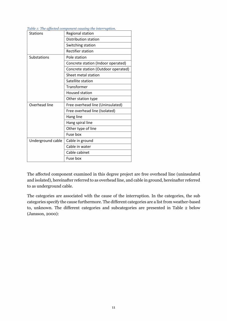
The affected component of the interruption is divided into categories. In each of the different

categories, there are subcategories where the affected component is further specified. This

keeps the DSOs aware of the number of interruptions categorized by component in the

electrical grid. The categories and the sub categories are presented in Table 1 (Jansson, 2000):

11

Table 1: The affected component causing the interruption.

Stations Regional station

Distribution station

Switching station

Rectifier station

Substations Pole station

Concrete station (Indoor operated)

Concrete station (Outdoor operated)

Sheet metal station

Satellite station

Transformer

Housed station

Other station type

Overhead line Free overhead line (Uninsulated)

Free overhead line (Isolated)

Hang line

Hang spiral line

Other type of line

Fuse box

Underground cable Cable in ground

Cable in water

Cable cabinet

Fuse box

The affected component examined in this degree project are free overhead line (uninsulated

and isolated), hereinafter referred to as overhead line, and cable in ground, hereinafter referred

to as underground cable.

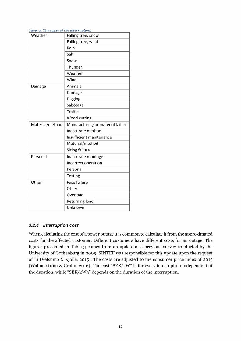
The categories are associated with the cause of the interruption. In the categories, the sub

categories specify the cause furthermore. The different categories are a list from weather-based

to, unknown. The different categories and subcategories are presented in Table 2 below

(Jansson, 2000):

12

Table 2: The cause of the interruption.

Weather Falling tree, snow

Falling tree, wind

Rain

Salt

Snow

Thunder

Weather

Wind

Damage Animals

Damage

Digging

Sabotage

Traffic

Wood cutting

Material/method Manufacturing or material failure

Inaccurate method

Insufficient maintenance

Material/method

Sizing failure

Personal Inaccurate montage

Incorrect operation

Personal

Testing

Other Fuse failure

Other

Overload

Returning load

Unknown

3.2.4 Interruption cost

When calculating the cost of a power outage it is common to calculate it from the approximated

costs for the affected customer. Different customers have different costs for an outage. The

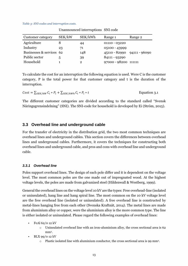
figures presented in Table 3 comes from an update of a previous survey conducted by the

University of Gothenburg in 2005, SINTEF was responsible for this update upon the request

of Ei (Vefsnmo & Kjolle, 2015). The costs are adjusted to the consumer price index of 2015

(Wallnerström & Grahn, 2016). The cost “SEK/kW” is for every interruption independent of

the duration, while “SEK/kWh” depends on the duration of the interruption.

13

Table 3: SNI-codes and interruption costs.

Unannounced interruptions SNI code

Customer category SEK/kW SEK/kWh Range 1 Range 2

Agriculture 8 44 01110 - 03220 Industry 23 71 05100 - 43999 Businesses & services 62 148 45110 - 82990 94111 - 96090

Public sector 5 39 84111 - 93290 Household 1 2 97000 - 98200 111111

To calculate the cost for an interruption the following equation is used. Were C is the customer

category, P is the total power for that customer category and t is the duration of the

interruption.

𝐶𝑜𝑠𝑡 = ∑ 𝐶𝑖 ∗ 𝑃𝑖𝑆𝐸𝐾/𝑘𝑊 + ∑ 𝐶𝑖 ∗ 𝑃𝑖 ∗ 𝑡𝑆𝐸𝐾/𝑘𝑊ℎ Equation 3.1

The different customer categories are divided according to the standard called “Svensk

Näringsgrensindelning” (SNI). The SNI-code for household is developed by Ei (Ström, 2015).

3.3 Overhead line and underground cable

For the transfer of electricity in the distribution grid, the two most common techniques are

overhead lines and underground cables. This section covers the differences between overhead

lines and underground cables. Furthermore, it covers the techniques for constructing both

overhead lines and underground cable, and pros and cons with overhead line and underground

cable.

3.3.1 Overhead line

Poles support overhead lines. The design of each pole differ and it is dependent on the voltage

level. The most common poles are the one made out of impregnated wood. At the highest

voltage levels, the poles are made from galvanized steel (Hildenwall & Westberg, 1999).

General the overhead lines on the voltage level 10 kV are the types: Free overhead-line (isolated

or uninsulated), hang line and hang spiral line. The most common on the 10 kV voltage level

are the free overhead line (isolated or uninsulated). A free overhead line is constructed by

metal-lines hanging free from each other (Svenska Kraftnät, 2014). The metal lines are made

from aluminium alloy or copper, were the aluminium alloy is the more common type. The line

is either isolated or uninsulated. Please regard the following examples of overhead lines:

• FeAl 62/0 12 kV

o Uninsulated overhead line with an iron-aluminium alloy, the cross sectional area is 62

mm2.

• BLX 99/0 12 kV

o Plastic isolated line with aluminium conductor, the cross sectional area is 99 mm2.

14

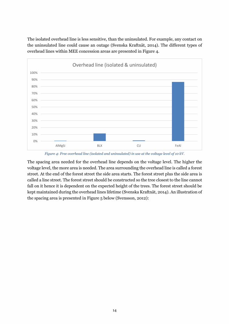
The isolated overhead line is less sensitive, than the uninsulated. For example, any contact on

the uninsulated line could cause an outage (Svenska Kraftnät, 2014). The different types of

overhead lines within MEE concession areas are presented in Figure 4.

Figure 4: Free overhead line (isolated and uninsulated) in use at the voltage level of 10 kV.

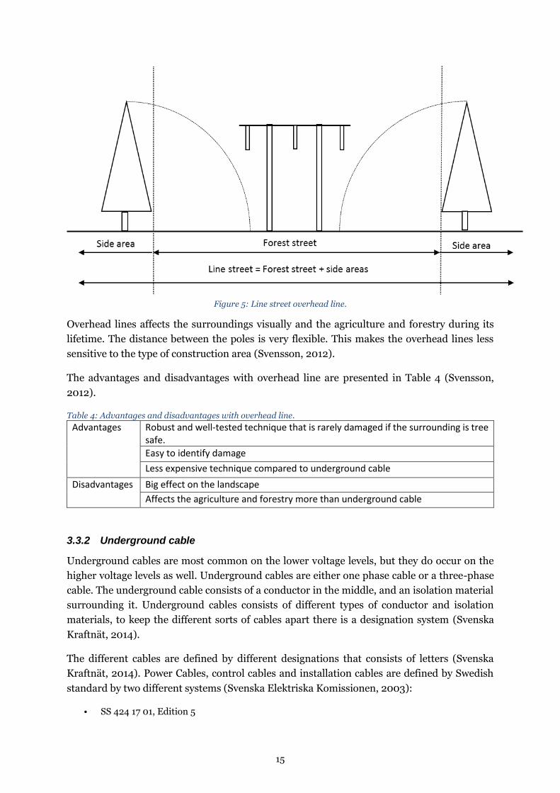
The spacing area needed for the overhead line depends on the voltage level. The higher the

voltage level, the more area is needed. The area surrounding the overhead line is called a forest

street. At the end of the forest street the side area starts. The forest street plus the side area is

called a line street. The forest street should be constructed so the tree closest to the line cannot

fall on it hence it is dependent on the expected height of the trees. The forest street should be

kept maintained during the overhead lines lifetime (Svenska Kraftnät, 2014). An illustration of

the spacing area is presented in Figure 5 below (Svensson, 2012):

0%

10%

20%

30%

40%

50%

60%

70%

80%

90%

100%

AlMgSi BLX CU FeAl

Overhead line (isolated & uninsulated)

15

Figure 5: Line street overhead line.

Overhead lines affects the surroundings visually and the agriculture and forestry during its

lifetime. The distance between the poles is very flexible. This makes the overhead lines less

sensitive to the type of construction area (Svensson, 2012).

The advantages and disadvantages with overhead line are presented in Table 4 (Svensson,

2012).

Table 4: Advantages and disadvantages with overhead line.

Advantages Robust and well-tested technique that is rarely damaged if the surrounding is tree safe.

Easy to identify damage

Less expensive technique compared to underground cable

Disadvantages Big effect on the landscape

Affects the agriculture and forestry more than underground cable

3.3.2 Underground cable

Underground cables are most common on the lower voltage levels, but they do occur on the

higher voltage levels as well. Underground cables are either one phase cable or a three-phase

cable. The underground cable consists of a conductor in the middle, and an isolation material

surrounding it. Underground cables consists of different types of conductor and isolation

materials, to keep the different sorts of cables apart there is a designation system (Svenska

Kraftnät, 2014).

The different cables are defined by different designations that consists of letters (Svenska

Kraftnät, 2014). Power Cables, control cables and installation cables are defined by Swedish

standard by two different systems (Svenska Elektriska Komissionen, 2003):

• SS 424 17 01, Edition 5

16

o This consists of a designation system that has been long used in Sweden and is applied

on national cable types. It applies also on CENELEC harmonized cable types that is not

covered in SS 424 07 02.

• SS 424 17 01, Edition 3

o This which fully reflects the designation system of CENELEC HD 361 S3 (System for

cable designation). It applies on CENELEC harmonized cable types with a rated voltage

level up to 450/750 V.

For a complete cable designation on a cable, the number of conductors, conductor area and in

some cases the area of the concentric conductor should be defined. The area of the concentric

conductor is separated from the conductor by a slash (/). Below, an example of the cable

designation be demonstrated (Svenska Elektriska Komissionen, 2003).

• AKKJ 3x150/41

o The cable have three isolated aluminium phase-conductor and one concentric

conductor with the area 41 mm. The isolation and the concentric conductor consists of

PVC.

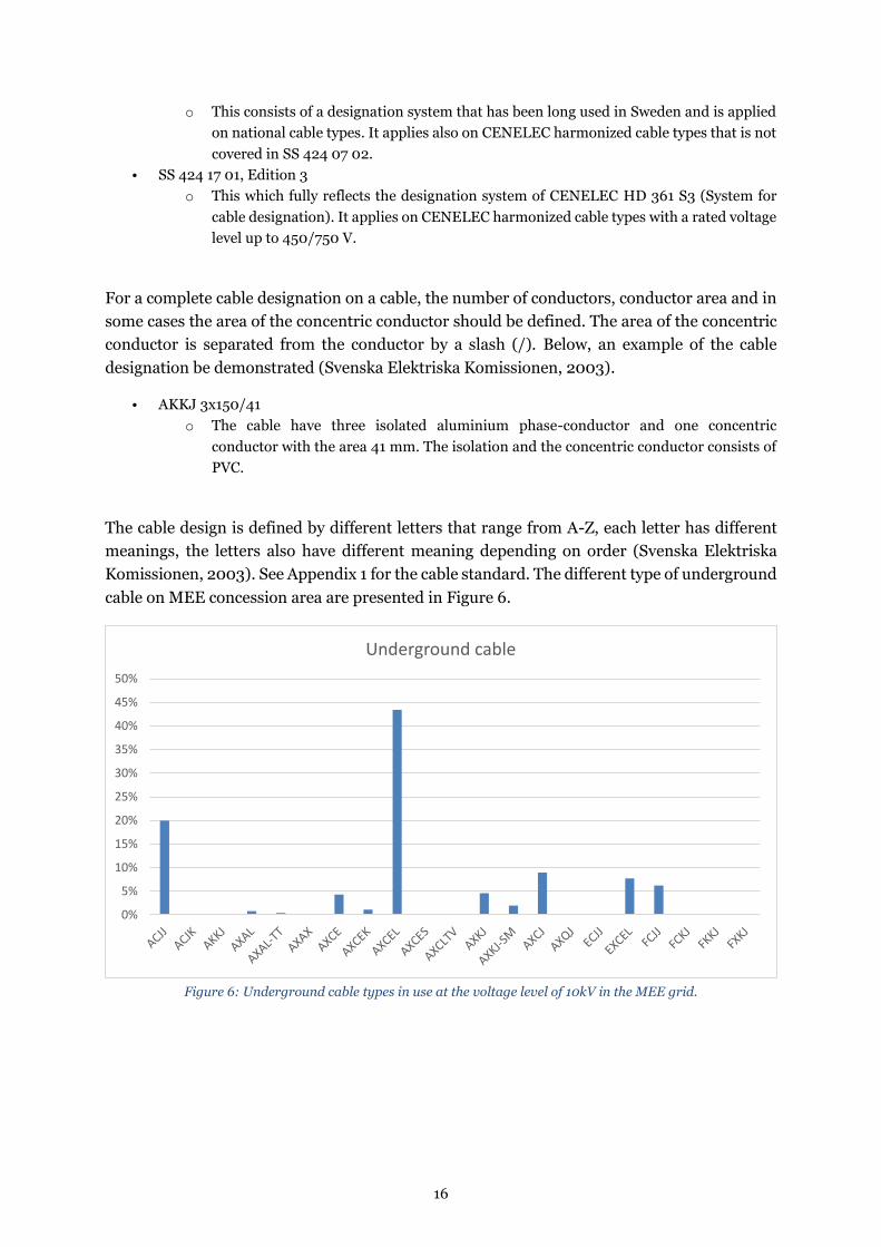
The cable design is defined by different letters that range from A-Z, each letter has different

meanings, the letters also have different meaning depending on order (Svenska Elektriska

Komissionen, 2003). See Appendix 1 for the cable standard. The different type of underground

cable on MEE concession area are presented in Figure 6.

Figure 6: Underground cable types in use at the voltage level of 10kV in the MEE grid.

0%

5%

10%

15%

20%

25%

30%

35%

40%

45%

50%

Underground cable

17

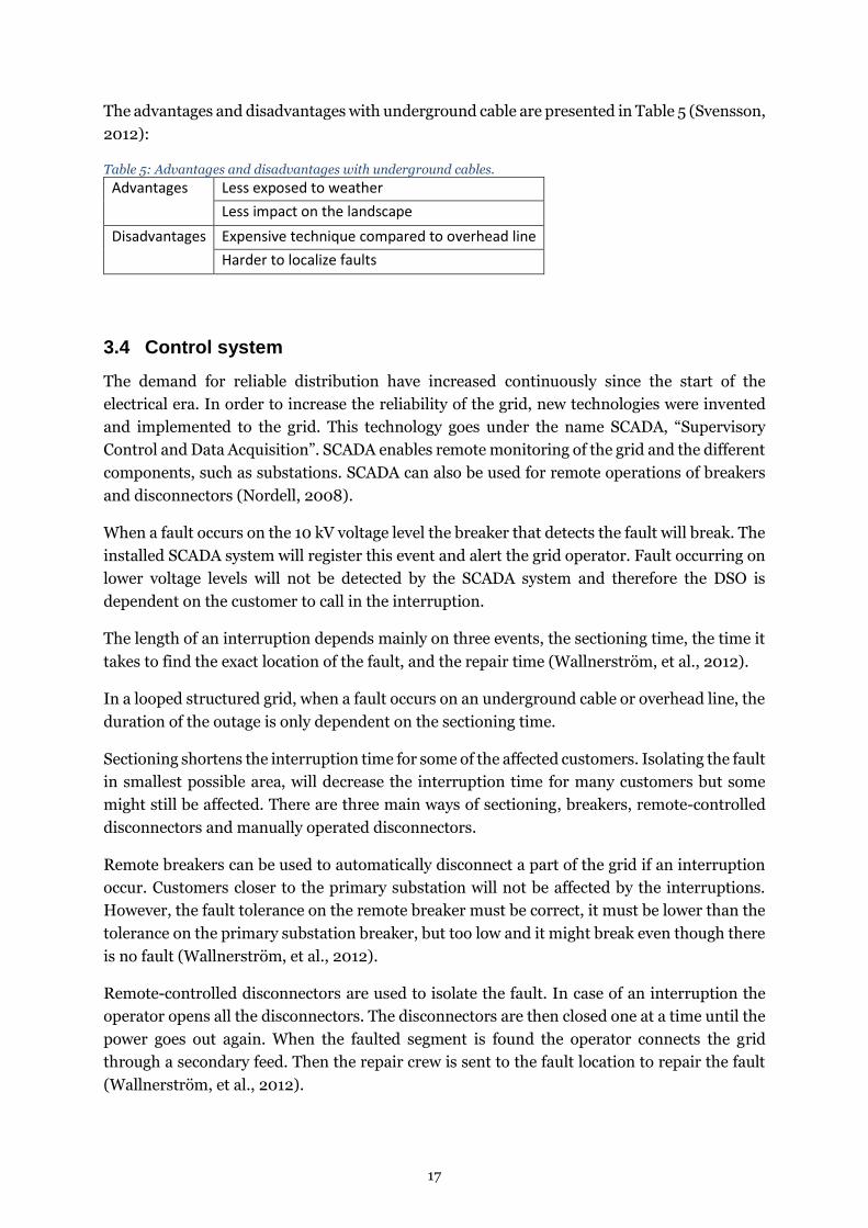
The advantages and disadvantages with underground cable are presented in Table 5 (Svensson,

2012):

Table 5: Advantages and disadvantages with underground cables.

Advantages Less exposed to weather

Less impact on the landscape

Disadvantages Expensive technique compared to overhead line

Harder to localize faults

3.4 Control system

The demand for reliable distribution have increased continuously since the start of the

electrical era. In order to increase the reliability of the grid, new technologies were invented

and implemented to the grid. This technology goes under the name SCADA, “Supervisory

Control and Data Acquisition”. SCADA enables remote monitoring of the grid and the different

components, such as substations. SCADA can also be used for remote operations of breakers

and disconnectors (Nordell, 2008).

When a fault occurs on the 10 kV voltage level the breaker that detects the fault will break. The

installed SCADA system will register this event and alert the grid operator. Fault occurring on

lower voltage levels will not be detected by the SCADA system and therefore the DSO is

dependent on the customer to call in the interruption.

The length of an interruption depends mainly on three events, the sectioning time, the time it

takes to find the exact location of the fault, and the repair time (Wallnerström, et al., 2012).

In a looped structured grid, when a fault occurs on an underground cable or overhead line, the

duration of the outage is only dependent on the sectioning time.

Sectioning shortens the interruption time for some of the affected customers. Isolating the fault

in smallest possible area, will decrease the interruption time for many customers but some

might still be affected. There are three main ways of sectioning, breakers, remote-controlled

disconnectors and manually operated disconnectors.

Remote breakers can be used to automatically disconnect a part of the grid if an interruption

occur. Customers closer to the primary substation will not be affected by the interruptions.

However, the fault tolerance on the remote breaker must be correct, it must be lower than the

tolerance on the primary substation breaker, but too low and it might break even though there

is no fault (Wallnerström, et al., 2012).

Remote-controlled disconnectors are used to isolate the fault. In case of an interruption the

operator opens all the disconnectors. The disconnectors are then closed one at a time until the

power goes out again. When the faulted segment is found the operator connects the grid

through a secondary feed. Then the repair crew is sent to the fault location to repair the fault

(Wallnerström, et al., 2012).

18

Manual disconnectors are operated in a similar way as remote-controlled disconnectors

described in the section above. However, since these disconnectors are manually operated a

fitter needs to be sent out directly to the affected grid section. Once on sight the fitter can start

to open and close disconnectors until the fault is located. Skilled and experienced fitters will

find the fault location quicker (Wallnerström, et al., 2012).

19

4 DISTRIBUTION SYSTEM RELIABILITY

4.1 DARWin-file

The original DARWin-file consisted of over 5000 interruptions, both announced and

unannounced. Excluding the interruptions stated by the constraints in the limitation, the

number of interruptions to examine was over 1000.

4.1.1 Overhead line

Approximately 750 interruptions occurred on both uninsulated and isolated overhead line.

Except for the information given in the DARWin-file was the following data collected using the

software Trimble NIS.

• Total length of overhead line and underground cable

• Start location of interruption (substation or disconnector)

• Overhead line

o Type

o Length

• Underground cable

o Type

o Length

• End location of interruption (substation or disconnector)

Grids containing overhead line often includes underground cable as well.

4.1.2 Underground cable

The remaining 300 outages occurred on underground cables. The description of the fault never

specified exactly which part of the cable that was the cause of the interruption. A cable section

between two substations usually consisted of several different types of underground cable. The

following data were collected with Trimble NIS.

• Total length

• Start location of the interruption (substation or disconnector)

• Number of joints

• Underground cable

o Type

o Length

• End location of interruption (substation or disconnector)

20

4.1.3 Evaluation of DARWin-file

Histograms over the interruptions on the examined components were made to see if there was

any relationship between the time of the day and the day of the week and the number of

interruptions.

4.2 Modelling of test grids

The primary substation that had the most number of interruptions reported for overhead line

and underground cables were examined. The most representative feeds when it comes to

reported outages were analysed for those primary substations.

4.2.1 Data collection

For constructing the test grids input data is needed, the input data is collected from the

software Trimble NIS. The following data were collected:

• Structure

o Radial

o Looped

o Double cable

• Overhead line and or underground cable

o Type

o Length

• Substation

o Type

o Number of customers

o Annual energy delivered

• Sectioning points

o Number of possible back-up feeds

• Interruptions

o Number of interruptions

o Cause of interruption

o Duration of interruption

o Affected customers

4.2.2 Classification of the test grids

To construct the test grids, the examined feeds are classified by two criteria’s. The main criteria

is the K-factor, and the sub criteria is the T-factor.

The K-factor states the composition of the grid.

𝐾 =𝑇𝑜𝑡𝑎𝑙 𝑙𝑒𝑛𝑔𝑡ℎ 𝑜𝑓 𝑢𝑛𝑑𝑒𝑟𝑔𝑟𝑜𝑢𝑛𝑑 𝑐𝑎𝑏𝑙𝑒

𝑇𝑜𝑡𝑎𝑙 𝑙𝑒𝑛𝑔𝑡ℎ 𝑜𝑓 𝑜𝑣𝑒𝑟ℎ𝑒𝑎𝑑 𝑙𝑖𝑛𝑒[−] Equation 4.1

The T-factor states the customer density of the grid.

21

𝑇 =𝑁𝑢𝑚𝑏𝑒𝑟 𝑜𝑓 𝑐𝑢𝑠𝑡𝑜𝑚𝑒𝑟𝑠

𝑇𝑜𝑡𝑎𝑙 𝑙𝑒𝑛𝑔𝑡ℎ 𝑜𝑓 𝑔𝑟𝑖𝑑 [

𝐶𝑢𝑠𝑡𝑜𝑚𝑒𝑟𝑠

𝑘𝑚] Equation 4.2

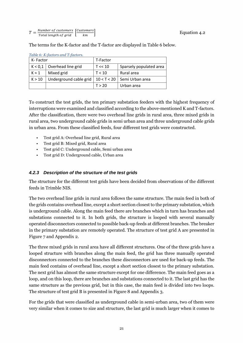
The terms for the K-factor and the T-factor are displayed in Table 6 below.

Table 6: K-factors and T-factors.

K- Factor T-Factor

K < 0,1 Overhead line grid T << 10 Sparsely populated area

K ≈ 1 Mixed grid T < 10 Rural area

K > 10 Underground cable grid 10 < T < 20 Semi Urban area

T > 20 Urban area

To construct the test grids, the ten primary substation feeders with the highest frequency of

interruptions were examined and classified according to the above-mentioned K and T-factors.

After the classification, there were two overhead line grids in rural area, three mixed grids in

rural area, two underground cable grids in semi urban area and three underground cable grids

in urban area. From these classified feeds, four different test grids were constructed.

• Test grid A: Overhead line grid, Rural area

• Test grid B: Mixed grid, Rural area

• Test grid C: Underground cable, Semi urban area

• Test grid D: Underground cable, Urban area

4.2.3 Description of the structure of the test grids

The structure for the different test grids have been decided from observations of the different

feeds in Trimble NIS.

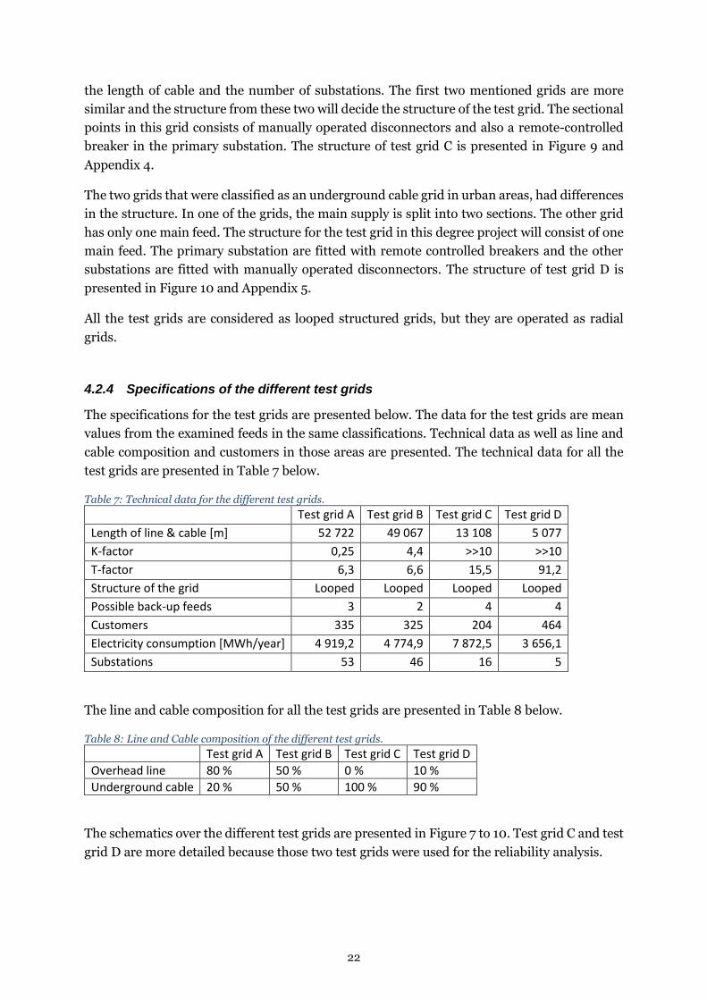
The two overhead line grids in rural area follows the same structure. The main feed in both of

the grids contains overhead line, except a short section closest to the primary substation, which

is underground cable. Along the main feed there are branches which in turn has branches and

substations connected to it. In both grids, the structure is looped with several manually

operated disconnectors connected to possible back-up feeds at different branches. The breaker

in the primary substation are remotely operated. The structure of test grid A are presented in

Figure 7 and Appendix 2.

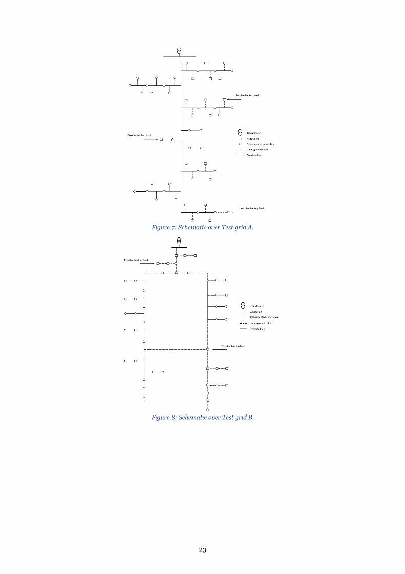
The three mixed grids in rural area have all different structures. One of the three grids have a

looped structure with branches along the main feed, the grid has three manually operated

disconnectors connected to the branches these disconnectors are used for back-up feeds. The

main feed contains of overhead line, except a short section closest to the primary substation.

The next grid has almost the same structure except for one difference. The main feed goes as a

loop, and on this loop, there are branches and substations connected to it. The last grid has the

same structure as the previous grid, but in this case, the main feed is divided into two loops.

The structure of test grid B is presented in Figure 8 and Appendix 3.

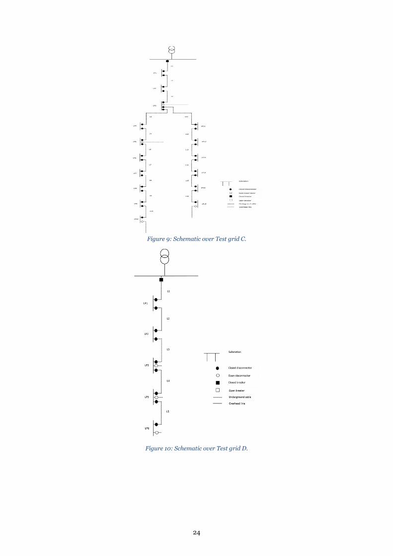
For the grids that were classified as underground cable in semi-urban area, two of them were

very similar when it comes to size and structure, the last grid is much larger when it comes to

22

the length of cable and the number of substations. The first two mentioned grids are more

similar and the structure from these two will decide the structure of the test grid. The sectional

points in this grid consists of manually operated disconnectors and also a remote-controlled

breaker in the primary substation. The structure of test grid C is presented in Figure 9 and

Appendix 4.

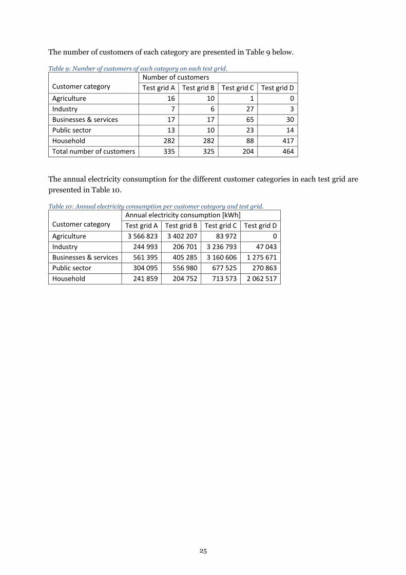
The two grids that were classified as an underground cable grid in urban areas, had differences

in the structure. In one of the grids, the main supply is split into two sections. The other grid

has only one main feed. The structure for the test grid in this degree project will consist of one

main feed. The primary substation are fitted with remote controlled breakers and the other

substations are fitted with manually operated disconnectors. The structure of test grid D is

presented in Figure 10 and Appendix 5.

All the test grids are considered as looped structured grids, but they are operated as radial

grids.

4.2.4 Specifications of the different test grids

The specifications for the test grids are presented below. The data for the test grids are mean

values from the examined feeds in the same classifications. Technical data as well as line and

cable composition and customers in those areas are presented. The technical data for all the

test grids are presented in Table 7 below.

Table 7: Technical data for the different test grids. Test grid A Test grid B Test grid C Test grid D

Length of line & cable [m] 52 722 49 067 13 108 5 077

K-factor 0,25 4,4 >>10 >>10

T-factor 6,3 6,6 15,5 91,2

Structure of the grid Looped Looped Looped Looped

Possible back-up feeds 3 2 4 4

Customers 335 325 204 464

Electricity consumption [MWh/year] 4 919,2 4 774,9 7 872,5 3 656,1

Substations 53 46 16 5

The line and cable composition for all the test grids are presented in Table 8 below.

Table 8: Line and Cable composition of the different test grids.

Test grid A Test grid B Test grid C Test grid D

Overhead line 80 % 50 % 0 % 10 %

Underground cable 20 % 50 % 100 % 90 %

The schematics over the different test grids are presented in Figure 7 to 10. Test grid C and test

grid D are more detailed because those two test grids were used for the reliability analysis.

23

Figure 7: Schematic over Test grid A.

Figure 8: Schematic over Test grid B.

24

Figure 9: Schematic over Test grid C.

Figure 10: Schematic over Test grid D.

25

The number of customers of each category are presented in Table 9 below.

Table 9: Number of customers of each category on each test grid.

Customer category

Number of customers

Test grid A Test grid B Test grid C Test grid D

Agriculture 16 10 1 0

Industry 7 6 27 3

Businesses & services 17 17 65 30

Public sector 13 10 23 14

Household 282 282 88 417

Total number of customers 335 325 204 464

The annual electricity consumption for the different customer categories in each test grid are

presented in Table 10.

Table 10: Annual electricity consumption per customer category and test grid.

Customer category

Annual electricity consumption [kWh]

Test grid A Test grid B Test grid C Test grid D

Agriculture 3 566 823 3 402 207 83 972 0

Industry 244 993 206 701 3 236 793 47 043

Businesses & services 561 395 405 285 3 160 606 1 275 671

Public sector 304 095 556 980 677 525 270 863

Household 241 859 204 752 713 573 2 062 517

26

4.3 Analytical reliability analysis

Test grids C and D will be used for the analytical reliability analysis. Test grid C and D has a

higher customer density than test grid A and B, this is the reason why they were chosen.

Analytical reliability analysis method is applicable when there is a high frequency of faults,

which makes it preferable on reliability calculations for the electrical grid (Wallnerström,

2011).

4.3.1 Failure rate

The number of interruptions on overhead line and underground cable between the years 2009-

2016 is taken from the DARWin-file. The length of the cables and overhead lines within the

MEE grid is also taken from the DARWin file. The data for calculation of the failure rate for

both the overhead line and underground cable are presented in Table 11 below.

Table 11: Length & number of interruptions on underground cables & overhead lines.

Year

Length [km] Number of interruptions

Cables OH-lines Cables OH-line

2009 1 358,1 466,5 39 118

2010 1 554,6 432,7 43 104

2011 1 565,8 418,0 48 114

2012 1 585,2 415,8 31 93

2013 1 616,2 398,7 44 84

2014 1 635,8 375,0 32 88

2015 1 720,2 347,4 33 67

2016 1 742,1 333,8 43 70

The average failure rate for underground cable and overhead line during the examined year

are calculated with equation 4.3 & 4.4. According to the data in Table 11 above, F is the number

of interruptions on each component for one year, and L is the total length for the same year.

𝜆𝐶𝑎𝑏𝑙𝑒 =∑ (

𝐹𝑌,𝐶𝑎𝑏𝑙𝑒𝐿𝑌,𝐶𝑎𝑏𝑙𝑒

)𝑌

∑ 𝑌𝑒𝑎𝑟𝑠 [

𝐹𝑎𝑖𝑙𝑢𝑟𝑒𝑠

𝑘𝑚,𝑌𝑒𝑎𝑟] Equation 4.3

𝜆𝑂𝐻 𝐿𝑖𝑛𝑒 =∑ (

𝐹𝑌,𝑂𝐻 𝐿𝑖𝑛𝑒𝐿𝑌,𝑂𝐻 𝐿𝑖𝑛𝑒

)𝑌

∑ 𝑌𝑒𝑎𝑟𝑠 [

𝐹𝑎𝑖𝑙𝑢𝑟𝑒𝑠

𝑘𝑚,𝑌𝑒𝑎𝑟] Equation 4.4

The calculated failure rates are presented in Table 12.

Table 12: Failure rates for overhead lines and underground cables. Overhead line Underground cable

Failure rate 0,2297 0,0247

Standard deviation ±0,024198 ±0,00433

27

4.3.2 Unavailability

The average repair time, 𝑟𝑖, for overhead line is according to Allan, et al, (1991), 5 hours and

for underground cable it is 30 hours. The average unavailability, 𝑈𝑖, in case of a failure on either

of these components is calculated using Equation 4.5.

𝑈𝑖 = 𝜆𝑖 ∗ 𝑟𝑖 [𝐻𝑜𝑢𝑟𝑠

𝑦𝑒𝑎𝑟] Equation 4.5

Since this degree project only handles the interruptions on overhead line and underground

cable the unavailability, 𝑈𝑖, can also be calculated with Equation 4.6, if the grid has the

possibility to be fed from a different primary substation feed. The unavailability time is then

dependent on the time it takes to isolate the faulted line and section the grid.

𝑈𝑖 = 𝜆𝑖 ∗ 𝑆𝑒𝑐𝑡𝑖𝑜𝑛𝑖𝑛𝑔 𝑡𝑖𝑚𝑒 [𝐻𝑜𝑢𝑟𝑠

𝑦𝑒𝑎𝑟] Equation 4.6

4.3.3 Reliability indicators

Reliability indicators are used for comparing the effect of interruptions between different grids

or grid sections. These reliability indicators are either weighted on number of customers

affected or the electric power affected. (Wallnerström, 2011)

The reliability indicators used in this degree project are presented in Equation 4.7 – 4.12 below,

where 𝑁𝑖 is the number of affected customers in each substation, 𝑈𝑖 is the unavailability

calculated from Equation 4.6.

System Average Interruption Frequency Index

𝑆𝐴𝐼𝐹𝐼 =∑ 𝑁𝑖𝜆𝑖𝑖

∑ 𝑁𝑖𝑖 [

𝐼𝑛𝑡𝑒𝑟𝑟𝑢𝑝𝑡𝑖𝑜𝑛𝑠

𝐶𝑢𝑠𝑡𝑜𝑚𝑒𝑟,𝑌𝑒𝑎𝑟] Equation 4.7

System Average Interruption Duration Index

𝑆𝐴𝐼𝐷𝐼 =∑ 𝑈𝑖𝑁𝑖𝑖

∑ 𝑁𝑖𝑖[

𝐻𝑜𝑢𝑟𝑠

𝐶𝑢𝑡𝑜𝑚𝑒𝑟,𝑌𝑒𝑎𝑟] Equation 4.8

Customer Average Interruption Duration Index

𝐶𝐴𝐼𝐷𝐼 =𝑆𝐴𝐼𝐷𝐼

𝑆𝐴𝐼𝐹𝐼[

𝐻𝑜𝑢𝑟𝑠

𝐼𝑛𝑡𝑒𝑟𝑟𝑢𝑝𝑡𝑖𝑜𝑛] Equation 4.9

Average Service Availability Index

𝐴𝑆𝐴𝐼 =8760∗∑ 𝑁𝑖−∑ 𝑁𝑖∗𝑈𝑖𝑖𝑖

8760∗∑ 𝑁𝑖𝑖 [𝑃𝑟𝑜𝑏𝑎𝑏𝑖𝑙𝑖𝑡𝑦] Equation 4.10

Average Service Unavailability Index

𝐴𝑆𝑈𝐼 = 1 − 𝐴𝑆𝐴𝐼 [𝑃𝑟𝑜𝑏𝑎𝑏𝑖𝑙𝑖𝑡𝑦] Equation 4.11

Energy Not Supplied

28

𝐸𝑁𝑆 =∑ 𝐴𝑛𝑛𝑢𝑎𝑙 𝑒𝑛𝑒𝑟𝑔𝑦𝑖∗𝑈𝑖𝑖

8760 [

𝑘𝑊ℎ

𝑦𝑒𝑎𝑟] Equation 4.12

4.3.4 Base scenario

In the base scenario, there is only one breaker in the grid. This breaker is installed at the

primary substation that feeds the grid. All the substations have manually operated

disconnectors. In event of a failure in the grid, the breaker in the primary substation will break,

and all the customers in the grid will have a power outage initially. The SCADA system will

alert the grid operator that a fault has occurred. The fitter is called to the grid section and

decides, based on information from SCADA and experience, where to start the sectioning. The

fitter then manually operates the disconnectors until the fault location is isolated and the

customers have their power back on. The sectioning time for an interruption is set to 2 hours

according to section 3.1.

4.3.5 Different sectioning times

The sectioning time at MEE is dependent on the experience of the operators and the fitters.

Therefore, the sectioning time is varied between 50 and 150 % of the original sectioning time.

This is done to see how much the sectioning time affects the cost and the reliability indicators.

The sectioning time for the different scenarios are presented in Table 13 below.

Table 13: Sectioning times for the different scenarios.

Scenario 1 (Base) 100% 2 hours

Scenario 2 50% 1 hour

Scenario 3 75% 1,5 hours

Scenario 4 125% 2,5 hours

Scenario 5 150% 3 hours

4.3.6 Design suggestion for Test grid C

There are several techniques and technologies to minimize the number of customers affected

by an interruption, SAIFI, as mentioned before removing overhead line and replacing it with

underground cable is one way of decreasing SAIFI. One other technology is to replace the

disconnectors in some of the substations with breakers that will break automatically in case of

an interruption. In this design suggestion, the substation LP3 in Test grid C is fitted with

breakers on the outgoing feeds. The purpose of the suggested design is to increase the overall

reliability of the test grid. The reason for the chosen design is because the grid splits into two

sections at LP3, and therefore, the potential for a reliability increase is assumed to be the

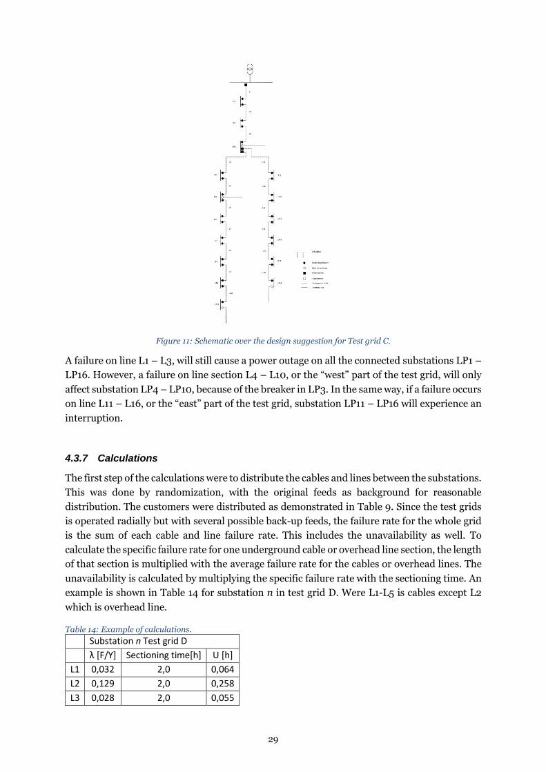
biggest at this point. In Figure 11, the schematics for this design are presented.

29

Figure 11: Schematic over the design suggestion for Test grid C.

A failure on line L1 – L3, will still cause a power outage on all the connected substations LP1 –

LP16. However, a failure on line section L4 – L10, or the “west” part of the test grid, will only

affect substation LP4 – LP10, because of the breaker in LP3. In the same way, if a failure occurs

on line L11 – L16, or the “east” part of the test grid, substation LP11 – LP16 will experience an

interruption.

4.3.7 Calculations

The first step of the calculations were to distribute the cables and lines between the substations.

This was done by randomization, with the original feeds as background for reasonable

distribution. The customers were distributed as demonstrated in Table 9. Since the test grids

is operated radially but with several possible back-up feeds, the failure rate for the whole grid

is the sum of each cable and line failure rate. This includes the unavailability as well. To

calculate the specific failure rate for one underground cable or overhead line section, the length

of that section is multiplied with the average failure rate for the cables or overhead lines. The

unavailability is calculated by multiplying the specific failure rate with the sectioning time. An

example is shown in Table 14 for substation n in test grid D. Were L1-L5 is cables except L2

which is overhead line.

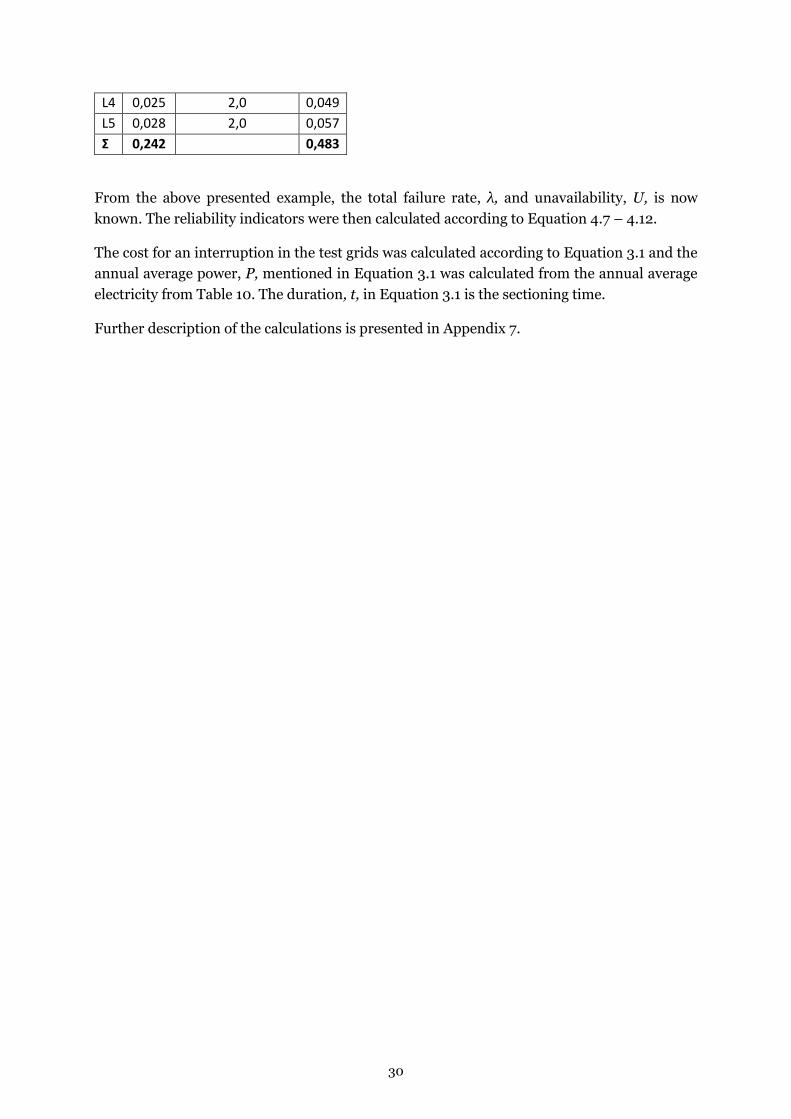
Table 14: Example of calculations. Substation n Test grid D λ [F/Y] Sectioning time[h] U [h]

L1 0,032 2,0 0,064

L2 0,129 2,0 0,258

L3 0,028 2,0 0,055

30

L4 0,025 2,0 0,049

L5 0,028 2,0 0,057

Σ 0,242

0,483

From the above presented example, the total failure rate, λ, and unavailability, U, is now

known. The reliability indicators were then calculated according to Equation 4.7 – 4.12.

The cost for an interruption in the test grids was calculated according to Equation 3.1 and the

annual average power, P, mentioned in Equation 3.1 was calculated from the annual average

electricity from Table 10. The duration, t, in Equation 3.1 is the sectioning time.

Further description of the calculations is presented in Appendix 7.

31

5 RESULTS

The results from this degree project are presented in the sections below. In section 5.1 different

histograms of the examined interruptions are presented. Sections 5.2 to 5.5 presents the results

from the test grids and calculations.

5.1 Histograms of the interruptions

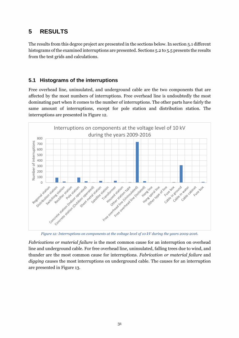
Free overhead line, uninsulated, and underground cable are the two components that are

affected by the most numbers of interruptions. Free overhead line is undoubtedly the most

dominating part when it comes to the number of interruptions. The other parts have fairly the

same amount of interruptions, except for pole station and distribution station. The

interruptions are presented in Figure 12.

Figure 12: Interruptions on components at the voltage level of 10 kV during the years 2009-2016.

Fabrications or material failure is the most common cause for an interruption on overhead

line and underground cable. For free overhead line, uninsulated, falling trees due to wind, and

thunder are the most common cause for interruptions. Fabrication or material failure and

digging causes the most interruptions on underground cable. The causes for an interruption

are presented in Figure 13.

0

100

200

300

400

500

600

700

800

Nu

mb

er o

f in

terr

up

tio

ns

Interruptions on components at the voltage level of 10 kV during the years 2009-2016

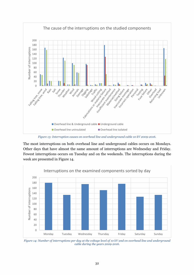
32

Figure 13: Interruption causes on overhead line and underground cable 10 kV 2009-2016.

The most interruptions on both overhead line and underground cables occurs on Mondays.

Other days that have almost the same amount of interruptions are Wednesday and Friday.

Fewest interruptions occurs on Tuesday and on the weekends. The interruptions during the

week are presented in Figure 14.

Figure 14: Number of interruptions per day at the voltage level of 10 kV and on overhead line and underground

cable during the years 2009-2016.

0

20

40

60

80

100

120

140

160

180

200

Nu

mb

er o

f in

terr

up

tio

ns

The cause of the interruptions on the studied components

Overhead line & Underground cable Underground cable

Overhead line uninsulated Overhead line isolated

0

20

40

60

80

100

120

140

160

180

200

Monday Tuesday Wednesday Thursday Friday Saturday Sunday

Nu

mb

er o

f in

terr

up

tio

ns

Interruptions on the examined components sorted by day

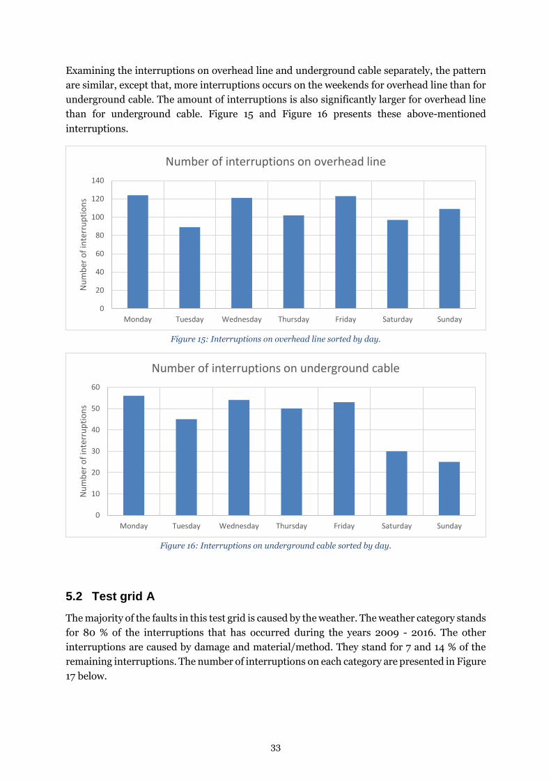
33

Examining the interruptions on overhead line and underground cable separately, the pattern

are similar, except that, more interruptions occurs on the weekends for overhead line than for

underground cable. The amount of interruptions is also significantly larger for overhead line

than for underground cable. Figure 15 and Figure 16 presents these above-mentioned

interruptions.

Figure 15: Interruptions on overhead line sorted by day.

Figure 16: Interruptions on underground cable sorted by day.

5.2 Test grid A

The majority of the faults in this test grid is caused by the weather. The weather category stands

for 80 % of the interruptions that has occurred during the years 2009 - 2016. The other

interruptions are caused by damage and material/method. They stand for 7 and 14 % of the

remaining interruptions. The number of interruptions on each category are presented in Figure

17 below.

0

20

40

60

80

100

120

140

Monday Tuesday Wednesday Thursday Friday Saturday Sunday

Nu

mb

er o

f in

terr

up

tio

ns

Number of interruptions on overhead line

0

10

20

30

40

50

60

Monday Tuesday Wednesday Thursday Friday Saturday Sunday

Nu

mb

er o

f in

terr

up

tio

ns

Number of interruptions on underground cable

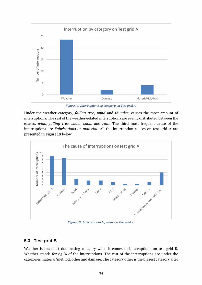
34

Figure 17: Interruptions by category on Test grid A.

Under the weather category, falling tree, wind and thunder, causes the most amount of

interruptions. The rest of the weather-related interruptions are evenly distributed between the

causes, wind, falling tree, snow, snow and rain. The third most frequent cause of the

interruptions are Fabrications or material. All the interruption causes on test grid A are

presented in Figure 18 below.

Figure 18: Interruptions by cause on Test grid A.

5.3 Test grid B

Weather is the most dominating category when it comes to interruptions on test grid B.

Weather stands for 65 % of the interruptions. The rest of the interruptions are under the

categories material/method, other and damage. The category other is the biggest category after

0

5

10

15

20

25

Weather Damage Material/Method

Nu

mb

er o

f in

terr

up

tio

ns

Interruption by category on Test grid A

0123456789

10

Nu

mb

er o

f in

terr

up

tio

ns

The cause of interruptions onTest grid A

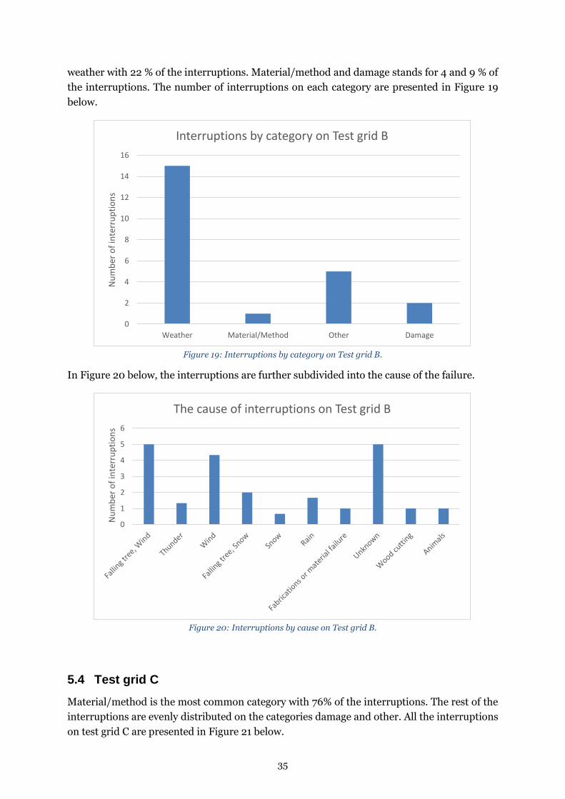
35

weather with 22 % of the interruptions. Material/method and damage stands for 4 and 9 % of

the interruptions. The number of interruptions on each category are presented in Figure 19

below.

Figure 19: Interruptions by category on Test grid B.

In Figure 20 below, the interruptions are further subdivided into the cause of the failure.

Figure 20: Interruptions by cause on Test grid B.

5.4 Test grid C

Material/method is the most common category with 76% of the interruptions. The rest of the

interruptions are evenly distributed on the categories damage and other. All the interruptions

on test grid C are presented in Figure 21 below.

0

2

4

6

8

10

12

14

16

Weather Material/Method Other Damage

Nu

mb

er o

f in

terr

up

tio

ns

Interruptions by category on Test grid B

0

1

2

3

4

5

6

Nu

mb

er o

f in

terr

up

tio

ns

The cause of interruptions on Test grid B

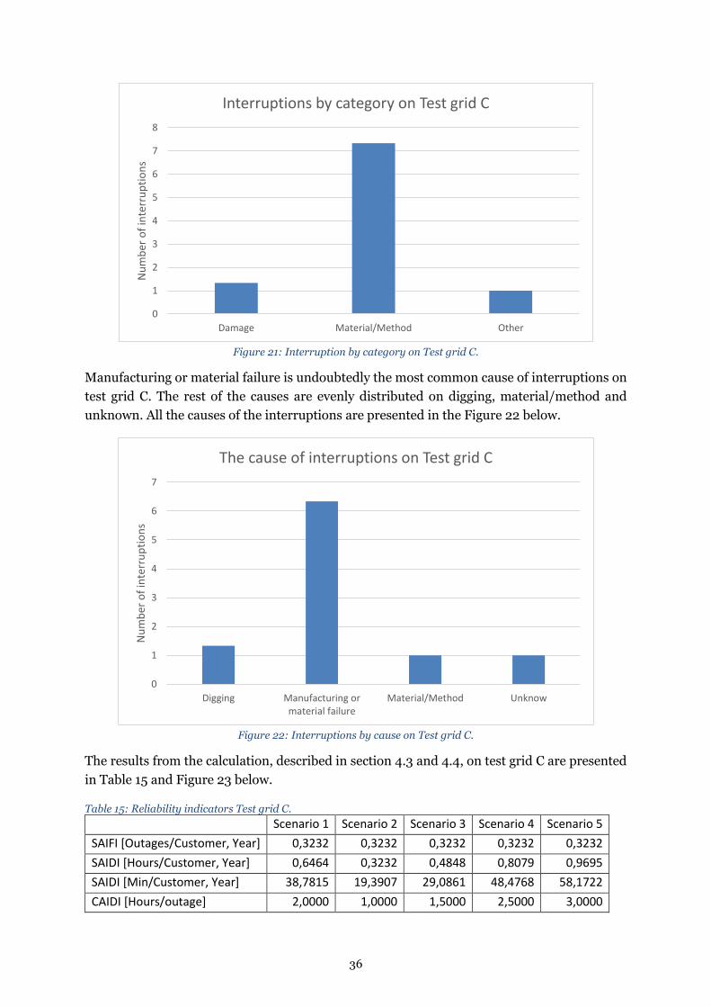
36

Figure 21: Interruption by category on Test grid C.

Manufacturing or material failure is undoubtedly the most common cause of interruptions on

test grid C. The rest of the causes are evenly distributed on digging, material/method and

unknown. All the causes of the interruptions are presented in the Figure 22 below.

Figure 22: Interruptions by cause on Test grid C.

The results from the calculation, described in section 4.3 and 4.4, on test grid C are presented

in Table 15 and Figure 23 below.

Table 15: Reliability indicators Test grid C.

Scenario 1 Scenario 2 Scenario 3 Scenario 4 Scenario 5

SAIFI [Outages/Customer, Year] 0,3232 0,3232 0,3232 0,3232 0,3232

SAIDI [Hours/Customer, Year] 0,6464 0,3232 0,4848 0,8079 0,9695

SAIDI [Min/Customer, Year] 38,7815 19,3907 29,0861 48,4768 58,1722

CAIDI [Hours/outage] 2,0000 1,0000 1,5000 2,5000 3,0000

0

1

2

3

4

5

6

7

8

Damage Material/Method Other

Nu

mb

er o

f in

terr

up

tio

ns

Interruptions by category on Test grid C

0

1

2

3

4

5

6

7

Digging Manufacturing ormaterial failure

Material/Method Unknow

Nu

mb

er o

f in

terr

up

tio

ns

The cause of interruptions on Test grid C

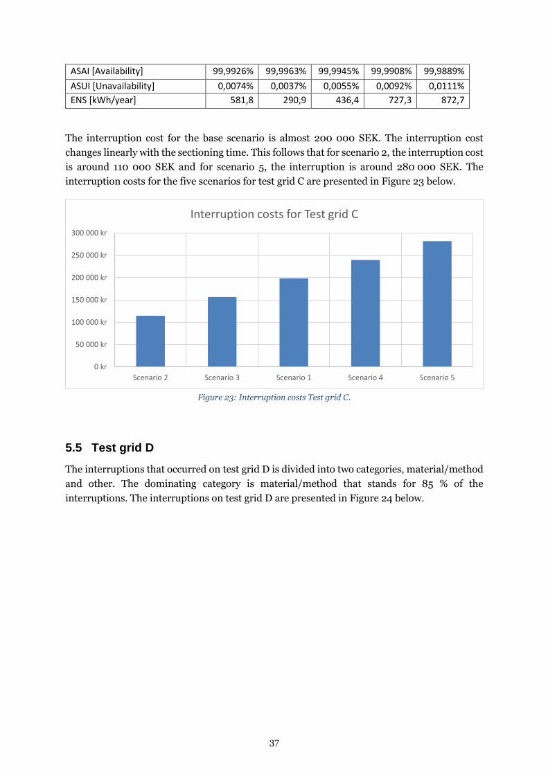
37

ASAI [Availability] 99,9926% 99,9963% 99,9945% 99,9908% 99,9889%

ASUI [Unavailability] 0,0074% 0,0037% 0,0055% 0,0092% 0,0111%

ENS [kWh/year] 581,8 290,9 436,4 727,3 872,7

The interruption cost for the base scenario is almost 200 000 SEK. The interruption cost

changes linearly with the sectioning time. This follows that for scenario 2, the interruption cost

is around 110 000 SEK and for scenario 5, the interruption is around 280 000 SEK. The

interruption costs for the five scenarios for test grid C are presented in Figure 23 below.

Figure 23: Interruption costs Test grid C.

5.5 Test grid D

The interruptions that occurred on test grid D is divided into two categories, material/method

and other. The dominating category is material/method that stands for 85 % of the

interruptions. The interruptions on test grid D are presented in Figure 24 below.

0 kr

50 000 kr

100 000 kr

150 000 kr

200 000 kr

250 000 kr

300 000 kr

Scenario 2 Scenario 3 Scenario 1 Scenario 4 Scenario 5

Interruption costs for Test grid C

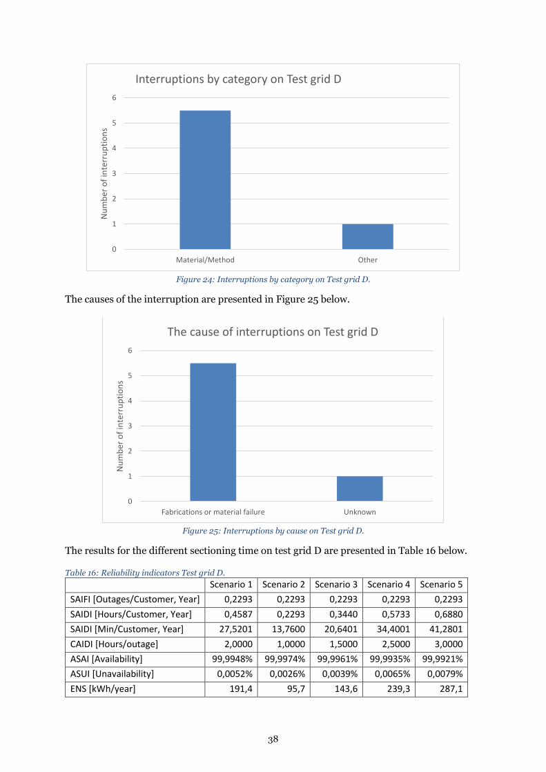
38

Figure 24: Interruptions by category on Test grid D.

The causes of the interruption are presented in Figure 25 below.

Figure 25: Interruptions by cause on Test grid D.

The results for the different sectioning time on test grid D are presented in Table 16 below.

Table 16: Reliability indicators Test grid D.

Scenario 1 Scenario 2 Scenario 3 Scenario 4 Scenario 5

SAIFI [Outages/Customer, Year] 0,2293 0,2293 0,2293 0,2293 0,2293

SAIDI [Hours/Customer, Year] 0,4587 0,2293 0,3440 0,5733 0,6880

SAIDI [Min/Customer, Year] 27,5201 13,7600 20,6401 34,4001 41,2801

CAIDI [Hours/outage] 2,0000 1,0000 1,5000 2,5000 3,0000

ASAI [Availability] 99,9948% 99,9974% 99,9961% 99,9935% 99,9921%

ASUI [Unavailability] 0,0052% 0,0026% 0,0039% 0,0065% 0,0079%

ENS [kWh/year] 191,4 95,7 143,6 239,3 287,1

0

1

2

3

4

5

6

Material/Method Other

Nu

mb

er o

f in

terr

up

tio

ns

Interruptions by category on Test grid D

0

1

2

3

4

5

6

Fabrications or material failure Unknown

Nu

mb

er o

f in

terr

up

tio

ns

The cause of interruptions on Test grid D

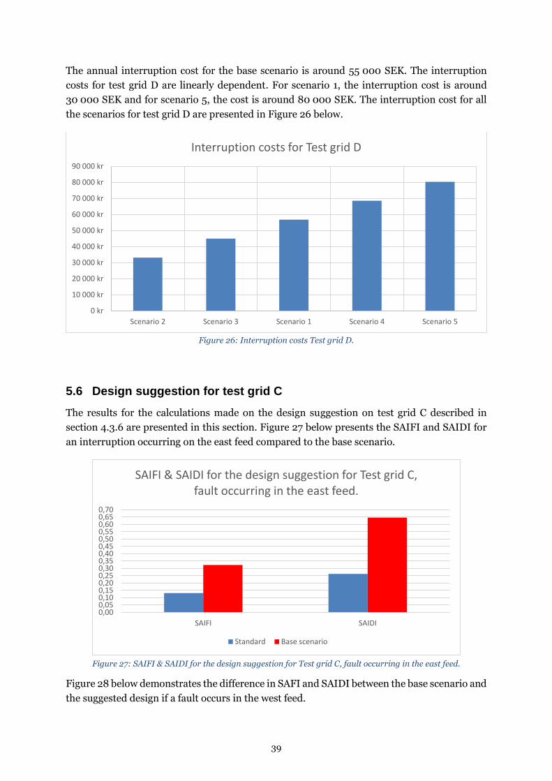
39

The annual interruption cost for the base scenario is around 55 000 SEK. The interruption

costs for test grid D are linearly dependent. For scenario 1, the interruption cost is around

30 000 SEK and for scenario 5, the cost is around 80 000 SEK. The interruption cost for all

the scenarios for test grid D are presented in Figure 26 below.

Figure 26: Interruption costs Test grid D.

5.6 Design suggestion for test grid C

The results for the calculations made on the design suggestion on test grid C described in

section 4.3.6 are presented in this section. Figure 27 below presents the SAIFI and SAIDI for

an interruption occurring on the east feed compared to the base scenario.

Figure 27: SAIFI & SAIDI for the design suggestion for Test grid C, fault occurring in the east feed.

Figure 28 below demonstrates the difference in SAFI and SAIDI between the base scenario and

the suggested design if a fault occurs in the west feed.

0 kr

10 000 kr

20 000 kr

30 000 kr

40 000 kr

50 000 kr

60 000 kr

70 000 kr

80 000 kr

90 000 kr

Scenario 2 Scenario 3 Scenario 1 Scenario 4 Scenario 5

Interruption costs for Test grid D

0,000,050,100,150,200,250,300,350,400,450,500,550,600,650,70

SAIFI SAIDI

SAIFI & SAIDI for the design suggestion for Test grid C, fault occurring in the east feed.

Standard Base scenario

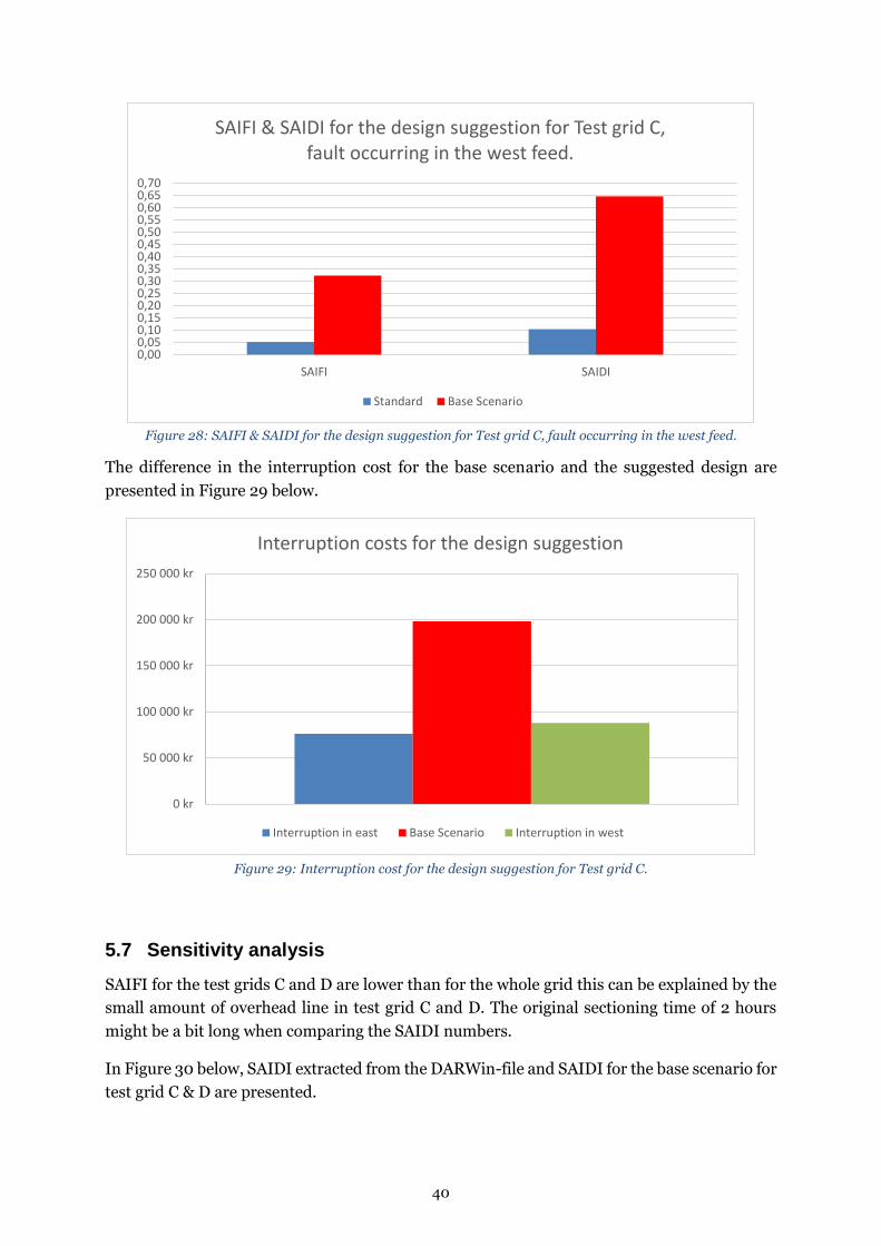
40

Figure 28: SAIFI & SAIDI for the design suggestion for Test grid C, fault occurring in the west feed.

The difference in the interruption cost for the base scenario and the suggested design are

presented in Figure 29 below.

Figure 29: Interruption cost for the design suggestion for Test grid C.

5.7 Sensitivity analysis

SAIFI for the test grids C and D are lower than for the whole grid this can be explained by the

small amount of overhead line in test grid C and D. The original sectioning time of 2 hours

might be a bit long when comparing the SAIDI numbers.

In Figure 30 below, SAIDI extracted from the DARWin-file and SAIDI for the base scenario for

test grid C & D are presented.

0,000,050,100,150,200,250,300,350,400,450,500,550,600,650,70

SAIFI SAIDI

SAIFI & SAIDI for the design suggestion for Test grid C, fault occurring in the west feed.

Standard Base Scenario

0 kr

50 000 kr

100 000 kr

150 000 kr

200 000 kr

250 000 kr

Interruption costs for the design suggestion

Interruption in east Base Scenario Interruption in west

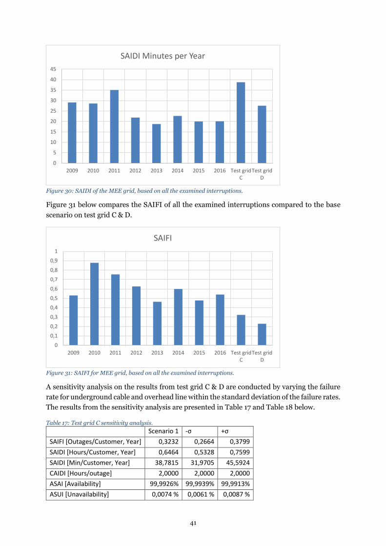
41

Figure 30: SAIDI of the MEE grid, based on all the examined interruptions.

Figure 31 below compares the SAIFI of all the examined interruptions compared to the base

scenario on test grid C & D.

Figure 31: SAIFI for MEE grid, based on all the examined interruptions.

A sensitivity analysis on the results from test grid C & D are conducted by varying the failure

rate for underground cable and overhead line within the standard deviation of the failure rates.

The results from the sensitivity analysis are presented in Table 17 and Table 18 below.

Table 17: Test grid C sensitivity analysis.

Scenario 1 -σ +σ

SAIFI [Outages/Customer, Year] 0,3232 0,2664 0,3799

SAIDI [Hours/Customer, Year] 0,6464 0,5328 0,7599

SAIDI [Min/Customer, Year] 38,7815 31,9705 45,5924

CAIDI [Hours/outage] 2,0000 2,0000 2,0000

ASAI [Availability] 99,9926% 99,9939% 99,9913%

ASUI [Unavailability] 0,0074 % 0,0061 % 0,0087 %

0

5

10

15

20

25

30

35

40

45

2009 2010 2011 2012 2013 2014 2015 2016 Test gridC

Test gridD

SAIDI Minutes per Year

0

0,1

0,2

0,3

0,4

0,5

0,6

0,7

0,8

0,9

1

2009 2010 2011 2012 2013 2014 2015 2016 Test gridC

Test gridD

SAIFI

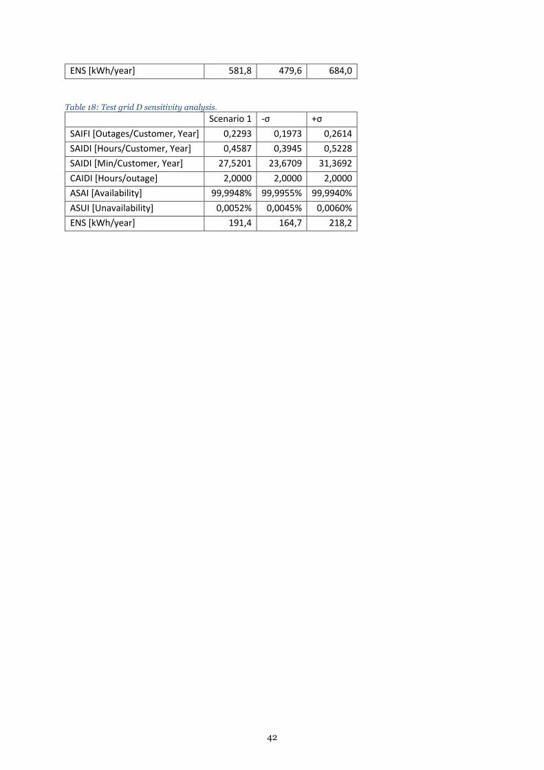
42

ENS [kWh/year] 581,8 479,6 684,0

Table 18: Test grid D sensitivity analysis.

Scenario 1 -σ +σ

SAIFI [Outages/Customer, Year] 0,2293 0,1973 0,2614

SAIDI [Hours/Customer, Year] 0,4587 0,3945 0,5228

SAIDI [Min/Customer, Year] 27,5201 23,6709 31,3692

CAIDI [Hours/outage] 2,0000 2,0000 2,0000

ASAI [Availability] 99,9948% 99,9955% 99,9940%

ASUI [Unavailability] 0,0052% 0,0045% 0,0060%

ENS [kWh/year] 191,4 164,7 218,2

43

6 DISCUSSION

6.1 Empirical research

The empirical research conducted in order to collect the data used for the test grids and

calculations were quite hard due to the fact that the DARWin file used were not as detailed as

one had hoped. Problems that occurred was due to the fact that all the examined interruption

was not properly reported. This lead to difficulties when searching for the affected part in

TRIMBLE. The examined interruptions occurred during the years 2009 to 2016, however,

during this period of time the grid have had some changes and the main changes are overhead

line that had been replaced with underground cable.

6.2 Result

From the histograms presented in section 5.1 it is clear that uninsulated overhead lines have a

lot more interruptions than isolated overhead line. This is due to the fact that the weather has

a significantly smaller impact on isolated overhead line, but also the fact that uninsulated is a

lot more common in the grid, which is shown in Figure 4.

The main reason for the dip in the number of interruptions on weekends on underground cable

is the fact that digging is primarily done during the weekdays. The reason for the dip on

Tuesdays on both overhead line and underground cable are a lot harder to explain.

The test grids constructed in the degree project are well suited for the reliability analysis

calculations. The faults occurring on the test grids are representable for what actually happens

on these kind of grids. The reliability of test grid A and B are heavily influenced by weather

related interruptions. This is because of the amount of overhead lines which are overall very

weather affected.

Test grid C and D which are almost completely constructed with underground cable are mainly

affected by material and methods related interruption. This category are the overall main

interruption cause on underground cable. However, only test grid C of these test grids are

affected by digging damages, which is very unusual for underground cable grids.

The reliability calculations computed on test grid C and D are showing reasonable numbers

compared to different similar studies. Quicker sectioning times decreases the SAIDI and

increases the availability ASAI in the grid. Shorter downtimes and therefore higher reliability

is something all DSOs are reaching for, because of the possibilities of bigger income frames in

future ex-ante regulations.

Since the interruption cost have a strict linear relationship to the duration of the interruption

the sectioning time have a big effect on the interruption cost. However, if the duration of the

interruption exceeds 12 hours the fee described in section 3.2.2 will take a huge part of the

interruption cost. These long outages are extremely rare when focusing on faults occurring on

44

overhead line and underground cables in looped structured grids, therefore, it is not handled

as a scenario for the models.

The design suggestion for Test grid C, where breakers are installed in substation LP3. The

reliability is increased a lot compared to the base scenario for the same test grid. Installing

breakers in an old substation may not be feasible depending on the structure of the substation.

Also, in reality the breakers will also have a failure rate, and therefore the real reliability

increase, might not be as significant as the result shown in this degree project.

45

7 CONCLUSIONS

The purpose of the degree project was to analyse interruption that has occurred on overhead

line and underground cable at voltage level at 10 kV within MEE distribution grid. Test grid

was developed for reliability analysis.

The conclusions drawn from the results are that the components that have the most amount of

interruptions are overhead line uninsulated and underground cable. This shows that the need

for studies like this one are significant and relevant.

The number of interruptions on overhead line and underground cable are evenly distributed

during the weekdays.

The primarily cause of an interruption on overhead line are weather based events. The main

causes of interruptions on underground cable grids are digging damages and fabrications or

material failures. The big share of digging failures are noticeable in Figure 16 where the number

of interruptions decreases during the weekends.

It is concluded that faster sectioning will lead to lower interruption costs. Installing breakers

at key points in the grid will help to isolate the fault, and decrease the number of affected

customers.

8 FUTURE WORK

Suggestions for future work concerning the outcome of this degree project are presented below.

Include more grid sections for more specified test grids. More underlying data for the

test grids will increase the accuracy of the test grids.

Including more data for the reliability calculations will help to improve the

understanding of the costs in case of an interruption. For example, including failure

rates for breakers, disconnectors and substations etc. will also increase the accuracy of

the test grids.

Different sectioning times dependent on where the fault occurs. For example, a fault on

a cable or overhead line far out on the grid may take longer time to find than a fault

close to the primary substation.

By introducing technology and automation to distribution grid the duration of an

interruption can be decreased. How much will it cost to decrease SAIDI by a minute in

different types of grids?

46

REFERENCES

Allan, R.N., Billinton, R., Sjarief, I., Goel, L. & So, K.S. (1991). A reliability test system for

educational purposes-basic distribution system data and results. IEEE Transactions on

Power Systems, 6, 813-820. https://doi.org/10.1109/59.76730

Banefelt, R. & Larsson, S., (2006). Kvalitén i elöverföringen - finns förutsättningar för en

effektiv tillsyn?, Stockholm: Riksrevisionen.

Cadini, F., Agliardi, G. L. & Zio, E., (2017). A modeling and simulation framework for the

reliability/availability assessment of a power transmission grid subject to cascading failures

under extreme weather conditions. Applied Energy, pp. 267-279.

Energiforsk, (2016). Energiforsk. [Online]

Available at: http://www.energiforsk.se/nyhetsarkiv/forbattring-av-avbrottsstatistik-i-

svenska-elnat/

[Använd 03 04 2017].

Energimyndigheten, (2015). Energimyndigheten. [Online]

Available at: http://www.energimyndigheten.se/trygg-energiforsorjning/kunskapsstod-till-

offentlig-sektor/lardomar-fran-intraffade-handelser/stormen-gudrun/

[Använd 07 04 2017].

Engblom, O. & Ueda, M., (2007). Representativa testnät för svenska eldistributionsnät,

Stockholm: Elforsk.

Heden, H. & Johansson, T., (2005). Energimarknad 2005 - Tema: Stormen Gudrun,

Stockholm: Statens Energimyndighet.

Hildenwall, B. & Westberg, S. B., (1999). Åldring av Luftledningsmateriel, Stockholm:

Elforsk.

Jansson, S., (2000). Kravspecifikation för DARWin, Stockholm: Sveriges Elleverantörer.

Konsumenternas Energimarknadsbyrå, (2017). Konsumenternas Energimarknadsbyrå.

[Online]

Available at: http://www.energimarknadsbyran.se/El/Elmarknaden/Elnatet/Elens-vag/

Lexholm, M., (2016). Nätuppbyggnad och automatiker för ökad tillgänglighet, Stockholm:

Energiforsk.

Morén, G., (2013). Energimarknadsinspektionens författningssamling, Eskilstuna: Swedish

Energy Market Inspectorate.

Mälarenergi AB, (2015). Så fungerar elnätet. [Online]

Available at: https://www.malarenergi.se/sv/privat/kunskapsbanken/el-och-elsakerhet/sa-

fungerar-elnatet/

[Använd 13 04 2017].

47

Nordell, D. E., (2008). Communication systems for Distribution Automation. IEEE/PES

Transmission and Distribution Conference and Exposition, pp. 1-14.

Pettersson, A., (2017). Energiföretagen. [Online]

Available at: https://www.energiforetagen.se/sa-fungerar-det/el/distribution/

[Använd 05 04 2017].

SFS 1997:857. Ellag. Stockholm: Miljö- och energidepartementet

Ström, L., (2015). Kvalitetsreglering av intäktsram – Reviderad metod inför tillsynsperiod

2016–2019, Eskilstuna: Swedish Energy Market Inspectorate.

Svenska Elektriska Komissionen, (2003). Power, control and house wiring cables - National

designations, u.o.: Svenska Elektriska Komissionen, SEK.

Svenska Kraftnät, (2014). Elnät i Fysisk Planering - Behandling av ledningar och stationer i

fysisk planering och tillståndsärenden, Stockholm: Svensk Energi.

Svensson, T., (2012). Luftledning eller markkabel - Hur ska framtidens regionnät byggas?,

Lund: Lunds Universitet.

Söder, L. & Amelin, M., (2011). Effektiv drift och planering av kraftsystem, Stockholm:

Kungliga tekniska högskolan Avdelningen för elektriska energisystem.

Tapper, M., (2016). DARWin Driftstörningsstatistik, Stockholm: Energiföretagen.

Torstensson, D. & Bollen, M., (2012). Leveranssäkerhet i elnäten 2010 Statistik och analys

av elavbrotten i Sverige, Eskilstuna: Swedish Energy Market Inspectorate.

Ueda, M., Engblom, O. & Alvehag, K., (2009). Representative test systems for Swedish

distribution networks. CIRED 2009 - 20th International Conference and Exhibition on

Electricity Distribution - Part 1, pp. 1-4.

Wallnerström, C. J., (2011). On Incentives affecting Risk and Asset Management of Power

Distribution, Stockholm: KTH - Royal Institute of Technology.

Wallnerström, C. J. & Grahn, E., (2016). Leveranssäkerhet i Sveriges elnät 2015, Eskilstuna:

Swedish Energy Markets Inspectorate.

Wallnerström, C. J., Stenberg, S. & Hilber, P., (2012). Fault Management at a Distribution

System Operator. Istanbul, 2012 IEEE 12th International Conference on Probabilistic

Methods Applied to Power Systems (PMAPS).

Vefsnmo, H. & Kjolle, G., (2015). Estimation of Cost of Electricity Interruptions in Sweden -

Interruption cost parameters based on the survey conducted by University of Gothenburg

from 2005, u.o.: SINTEF.

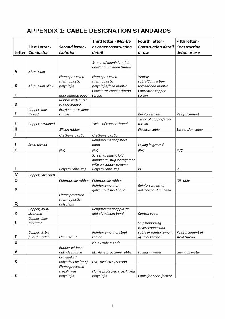
1

APPENDIX 1: CABLE DESIGNATION STANDARDS

Letter First Letter - Conductor

Second letter - Isolation

Third letter - Mantle or other construction detail

Fourth letter - Construction detail or use

Fifth letter - Construction detail or use

A Aluminium

Screen of aluminium foil and/or aluminium thread

B Aluminium alloy

Flame protected thermoplastic polyolefin

Flame protected thermoplastic polyolefin/lead mantle

Vehicle cable/Connection thread/lead mantle

C Impregnated paper Concentric copper thread screen

Concentric copper screen

D

Rubber with outer rubber mantle

E Copper, one thread

Ethylene-propylene rubber Reinforcement Reinforcement

F Copper, stranded Twine of copper thread Twine of copper/steel thread

H Silicon rubber Elevator cable Suspension cable

I Urethane plastic Urethane plastic

J Steal thread

Reinforcement of steel band Laying in ground

K PVC PVC PVC PVC

L Polyethylene (PE)

Screen of plastic laid aluminium strip ev together with an copper screen / Polyethylene (PE) PE PE

M Copper, Stranded O Chloroprene rubber Chloroprene rubber Oil cable

P

Reinforcement of galvanized steel band

Reinforcement of galvanized steel band

Q

Flame protected thermoplastic polyolefin

R Copper, multi stranded

Reinforcement of plastic laid aluminium band Control cable

S Copper, fine-threaded Self-supporting

T Copper, Extra fine-threaded Fluorescent

Reinforcement of steal thread

Heavy connection cable or reinforcement of steal thread

Reinforcement of steal thread

U No outside mantle

V

Rubber without outside mantle Ethylene-propylene rubber Laying in water Laying in water

X

Crosslinked polyethylene (PEX) PVC, oval cross section

Z

Flame protected crosslinked polyolefin

Flame protected crosslinked polyolefin Cable for neon-facility

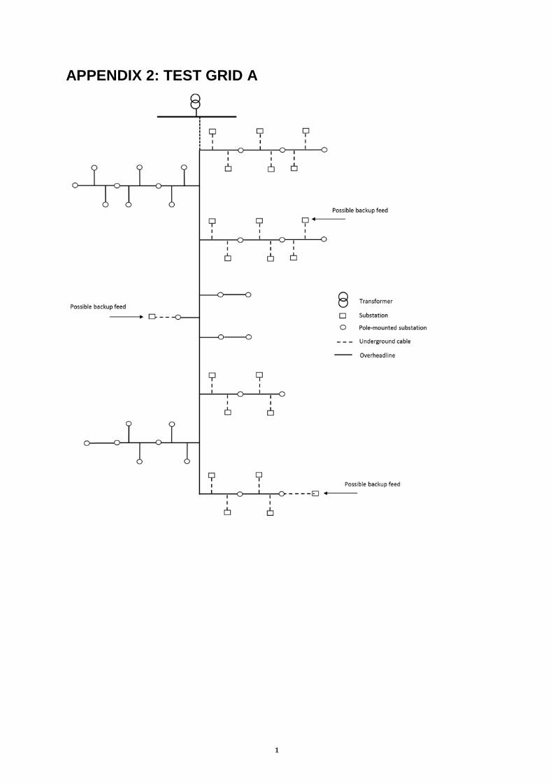
1

APPENDIX 2: TEST GRID A

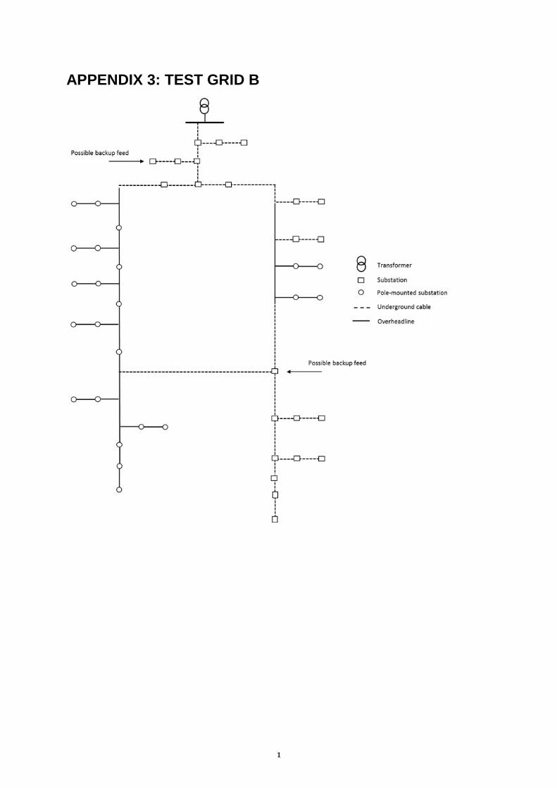
1

APPENDIX 3: TEST GRID B

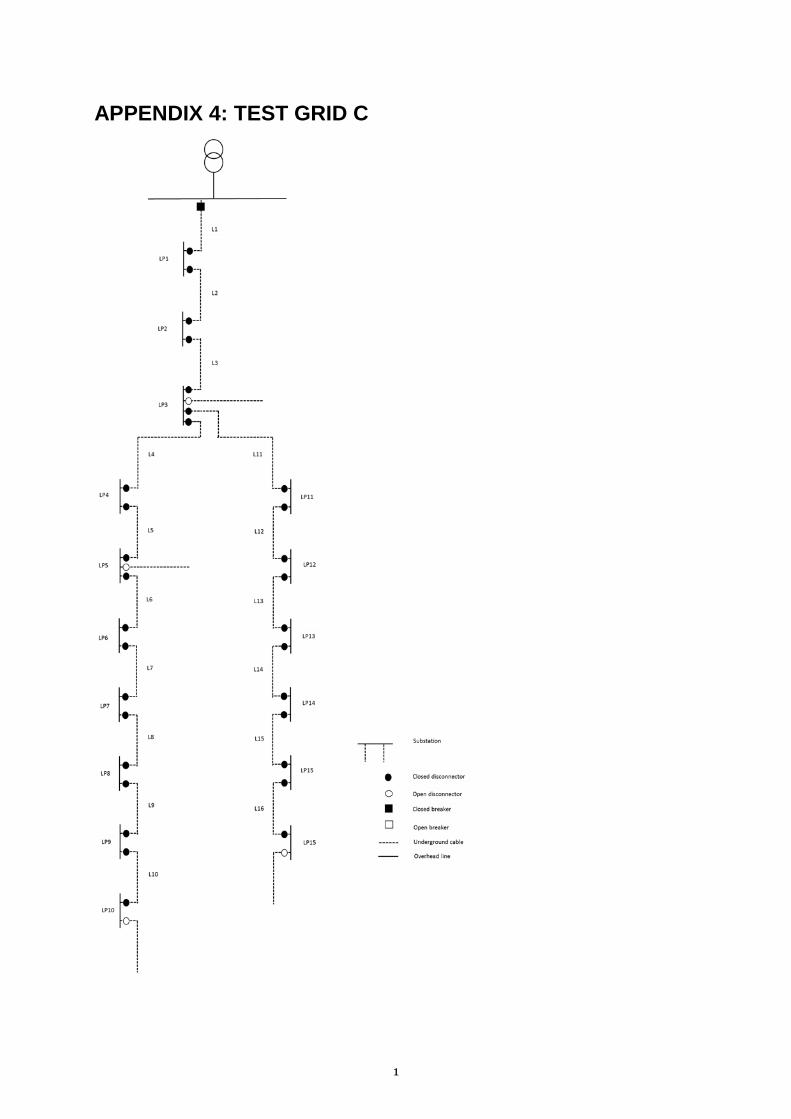
1

APPENDIX 4: TEST GRID C

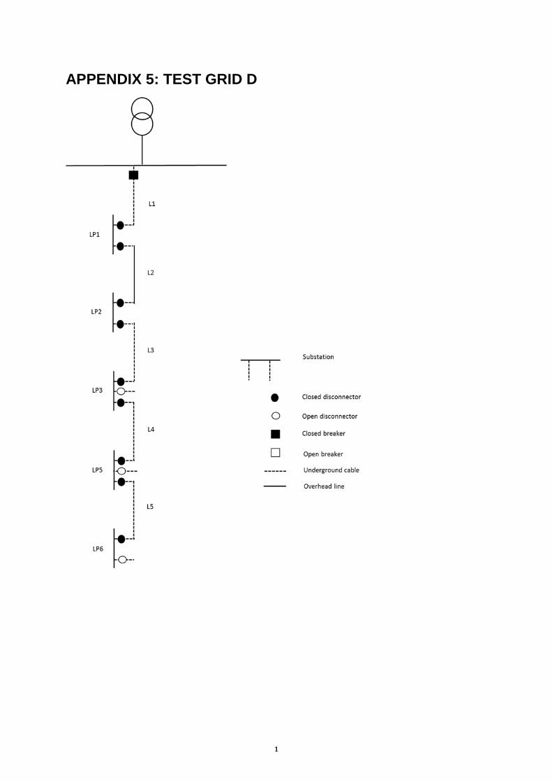
1

APPENDIX 5: TEST GRID D

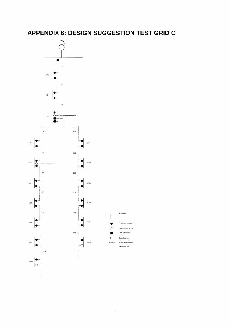
1

APPENDIX 6: DESIGN SUGGESTION TEST GRID C

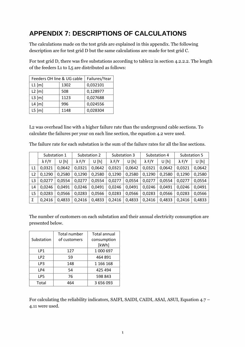
1

APPENDIX 7: DESCRIPTIONS OF CALCULATIONS

The calculations made on the test grids are explained in this appendix. The following

description are for test grid D but the same calculations are made for test grid C.

For test grid D, there was five substations according to table12 in section 4.2.2.2. The length

of the feeders L1 to L5 are distributed as follows:

Feeders OH line & UG cable Failures/Year

L1 [m] 1302 0,032101

L2 [m] 508 0,128977

L3 [m] 1123 0,027688

L4 [m] 996 0,024556

L5 [m] 1148 0,028304

L2 was overhead line with a higher failure rate than the underground cable sections. To

calculate the failures per year on each line section, the equation 4.2 were used.

The failure rate for each substation is the sum of the failure rates for all the line sections.

Substation 1 Substation 2 Substation 3 Substation 4 Substation 5

λ F/Y U [h] λ F/Y U [h] λ F/Y U [h] λ F/Y U [h] λ F/Y U [h]

L1 0,0321 0,0642 0,0321 0,0642 0,0321 0,0642 0,0321 0,0642 0,0321 0,0642

L2 0,1290 0,2580 0,1290 0,2580 0,1290 0,2580 0,1290 0,2580 0,1290 0,2580

L3 0,0277 0,0554 0,0277 0,0554 0,0277 0,0554 0,0277 0,0554 0,0277 0,0554

L4 0,0246 0,0491 0,0246 0,0491 0,0246 0,0491 0,0246 0,0491 0,0246 0,0491

L5 0,0283 0,0566 0,0283 0,0566 0,0283 0,0566 0,0283 0,0566 0,0283 0,0566

Σ 0,2416 0,4833 0,2416 0,4833 0,2416 0,4833 0,2416 0,4833 0,2416 0,4833

The number of customers on each substation and their annual electricity consumption are

presented below.

Substation

Total number of customers

Total annual consumption

[kWh]

LP1 127 1 000 697

LP2 59 464 891

LP3 148 1 166 168

LP4 54 425 494

LP5 76 598 843

Total 464 3 656 093

For calculating the reliability indicators, SAIFI, SAIDI, CAIDI, ASAI, ASUI, Equation 4.7 –

4.11 were used.

2

For calculating the last reliability indicator, Energy not Supplied (ENS), Equation 4.12 were

used. For this equation, the annual energy for each substation were used.

For the cost of the interruption Equation 3.1 were used, with the duration of the interruption

set to the sectioning time. Because in this way the cost for an interruption was calculated,

setting the duration to U, will calculate the average annual cost for interruptions.

For the design suggestion for Test grid C, the same calculations and equations were used.

However, the failure rate and unavailability for each substation is dependent on were the

failure occurs. For example, if a failure occurs on line L4 – L10, the breaker in substation LP3

will open and substation LP4 – LP10 will experience an interruption. If a failure occurs on

L1-L3, the breaker in the primary substation will open and therefore all the substations in the

test grid will experience an interruption until the fault section is isolated.

P.O. Box 883, SE-721 23 Västerås, Sweden Phone: +46 21 101 300 P.O. Box 325, SE-631 05 Eskilstuna, Sweden Phone: +46 16 153 600

E-mail: info@mdh.se Webb: www.mdh.se