Approved by Date

Ralf Hartings 2002-11-27 Reviewed by No. of pages of text

Mats Häger 94 STRI project number No. of suppl. pages

3261 11 + 21 Your ref

Test and evaluation of voltage dip immunity

Author Thomas Andersson Daniel Nilsson

Distribution Chalmers, Inst. Elteknik, Jaap Daalder Vattenfall Sveanät, Åke Ceder

R02-093 page ii (xi)

R02-093 page iii (xi)

Abstract One of the largest power quality problem today is voltage dips. Each year voltage dips cause disturbances in industries, resulting in large economical losses. Today these problems are often solved as they are discovered, and very often the equipment selected for improved immunity are based on experience and opinions rather than a traceable technical analysis. One related problem to voltage dips is that there are no standards covering the complete issue, e.g. there are no descriptions on how to test and present the immunity in a three-phase system.

This report presents a structured way of working with voltage dips in order to obtain the voltage dip immunity and related costs. Improving the immunity of a plant must be an ongoing work involving the whole process rather than just separately identified malfunctions. Before deciding to perform a mitigation action, two analyses should be carried out. First, a study of the voltage dip characteristics affecting the site, which will provide information of the voltage dips, types, magnitude, activity, etc. Secondly a work to identify the processes causing the highest cost, and estimating the immunity level of the site has to be done.

The proposed method is based on three indices; cost, fault frequency and the interconnection between processes. The different indices will provide knowledge of which process that can have the highest cost assigned due to a voltage dip caused shutdown. Knowing the cost for the voltage dip, evaluation of different mitigation actions can be calculated in order to find them motivated or not. Finally, the report briefly presents some frequent mitigation methods and measurements results from field measurement at the pulp and paper plant Gruvön.

R02-093 page iv (xi)

R02-093 page v (xi)

Preface

This report is the result of a master thesis work done by two students from Chalmers University of Technology. The work was performed at the research company STRI AB and financed by Vatenfall AB.

R02-093 page vi (xi)

R02-093 page vii (xi)

Acknowledgements

The authors would like to thank the following persons for contributing and making this report possible.

Mats Häger, tutor at STRI.

Prof. Jaap Daalder, examiner Chalmers.

Åke Ceder, Vattenfall AB.

Prof. Math Bollen, Chalmers.

Thomas Sandberg, Gruvön (pulp and paper mill).

Anders Stavhagen, Väröbruk (pulp mill).

R02-093 page viii (xi)

R02-093 page ix (xi)

Table of Contents Page

Title page .................................................................................................................................i Abstract..................................................................................................................................iii Preface ....................................................................................................................................v Acknowledgements...............................................................................................................vi 1 INTRODUCTION ON VOLTAGE DIPS................................................................................................................1

1.1. DEFINITION OF VOLTAGE DIPS...............................................................................................................................1 1.1.1 The IEEE Std. 1159 definitions ....................................................................................................................2 1.1.2 The IEC 61000-2-8 definitions .....................................................................................................................2

1.2. CHARACTERISATION OF A VOLTAGE DIP ...............................................................................................................3 1.3. SOURCE AND OCCURRENCE...................................................................................................................................5 1.4. PROPAGATION.......................................................................................................................................................5

1.4.1 Influence of the system design ......................................................................................................................6 1.4.2 Voltage dip classification .............................................................................................................................6

1.5. CONSEQUENSES DUE TO VOLTAGE DIPS.................................................................................................................9 1.5.1 Voltage dip related problems in different types of industries.......................................................................9 1.5.2 Costs caused by voltage dips in different types of industries. ....................................................................12

1.6. SENSITIVE EQUIPMENT........................................................................................................................................13 1.6.1 Computers ..................................................................................................................................................14 1.6.2 AC adjustable speed drives ........................................................................................................................15 1.6.3 DC adjustable speed drives........................................................................................................................17 1.6.4 Induction motors ........................................................................................................................................19 1.6.5 Synchronous machines ...............................................................................................................................21 1.6.6 Machine tools .............................................................................................................................................24 1.6.7 Automation equipment (PLC).....................................................................................................................24 1.6.8 AC Contactors............................................................................................................................................25 1.6.9 Lighting (illumination) ...............................................................................................................................25

1.7. STANDARDS AND TECHNICAL REPORTS ASSOCIATED WITH VOLTAGE DIPS..........................................................26 1.7.1 The use of standards...................................................................................................................................26 1.7.2 Available standards....................................................................................................................................26 1.7.3 Differences between the standards.............................................................................................................33

1.8. CONCLUSION.......................................................................................................................................................33 1.8.1 Description of voltage dips ........................................................................................................................33 1.8.2 Equipment sensitivity..................................................................................................................................34 1.8.3 Standards ...................................................................................................................................................34

2 CHARACTERISATION OF VOLTAGE DIP ACTIVITY AT THE SITE .......................................................36 2.1. VOLTAGE DIP SOURCES.......................................................................................................................................36

2.1.1 Remotely injected voltage dips ...................................................................................................................36 2.1.2 Locally injected voltage dips......................................................................................................................36

2.2. MEASUREMENT...................................................................................................................................................36 2.3. DETERMINING VOLTAGE DIP ACTIVITY ...............................................................................................................38

2.3.1 Data from measurements ...........................................................................................................................38 2.3.2 Data from stochastic predictions of voltage dips .......................................................................................38 2.3.3 Typical data................................................................................................................................................39

2.4. CHARACTERISATION WITH CHARTS AND VOLTAGE DIP INDICES..........................................................................39 2.4.1 Voltage-duration chart...............................................................................................................................39 2.4.2 SARFI (x)....................................................................................................................................................41 2.4.3 Sag score ....................................................................................................................................................42 2.4.4 UNIPEDE...................................................................................................................................................43 2.4.5 ESKOM Voltage Dip Table ........................................................................................................................44 2.4.6 Loss of energy ............................................................................................................................................44 2.4.7 Three-phase-voltages versus time plot for representation .........................................................................45 2.4.8 RMS-voltages and phase-angle versus time plot for representation ..........................................................46

R02-093 page x (xi)

2.4.9 Symmetrical components for representation ............................................................................................. 46 2.5. PROPOSED REPRESENTATION OF VOLTAGE DIPS ................................................................................................. 47

2.5.1 Equipment sensitive to loss of energy ........................................................................................................ 47 2.5.2 Equipment sensitive to phase-angle-jump ................................................................................................. 48 2.5.3 Equipment sensitive to other parameters................................................................................................... 48

3 METHOD FOR EVALUATION OF AN INDUSTRIAL PROCESS ACCORDING TO VOLTAGE DIPS.. 51 3.1. DEFINING PROCESSES ......................................................................................................................................... 51 3.2. CONSTRUCTION AND USE OF COST INDEX ........................................................................................................... 53 3.3. CONSTRUCTION AND USE OF THE FAULT INDEX.................................................................................................. 54 3.4. CONSTRUCTION OF A INTERLOCKING CHART...................................................................................................... 55 3.5. EVALUATION OF THE INDICES AND RANKING THE PROCESSES ............................................................................ 56

3.5.1 Evaluation according to the most expensive process................................................................................. 56 3.5.2 Evaluation according to the process with lowest immunity....................................................................... 57 3.5.3 Result of evaluation ................................................................................................................................... 58

3.6. DIVIDING SELECTED PROCESSES INTO SUB-PROCESSES FOR IMMUNITY-STUDIES ................................................ 58 3.7. CONSTRUCTION OF A SUB COST-INDEX............................................................................................................... 58 3.8. CONSTRUCTION OF A SUB FAULT-INDEX............................................................................................................. 59 3.9. CONSTRUCTION OF A SUB-PROCESS INTERLOCKING CHART................................................................................ 59 3.10. ESTIMATING THE IMMUNITY AND THE COST OF A SUB-PROCESS ..................................................................... 60

3.10.1 The sub-process with the lowest voltage dip immunity.............................................................................. 60 3.10.2 The sub-process with the highest cost due to voltage dips ........................................................................ 60

3.11. AVAILABLE VOLTAGE DIP IMMUNITY DATA FOR THE EQUIPMENT .................................................................. 60 3.12. PERFORMING TESTS........................................................................................................................................ 61

3.12.1 Number of phases ...................................................................................................................................... 61 3.12.2 Type of voltage dip .................................................................................................................................... 62 3.12.3 Duration of the voltage dip........................................................................................................................ 62 3.12.4 Criteria for normal operation.................................................................................................................... 63 3.12.5 Test standards............................................................................................................................................ 63 3.12.6 Test equipment........................................................................................................................................... 63 3.12.7 Test protocol .............................................................................................................................................. 64 3.12.8 Proposed test ............................................................................................................................................. 64

3.13. EVALUATING TEST RESULTS........................................................................................................................... 65 3.13.1 Single-phase test representation and evaluation ....................................................................................... 65 3.13.2 Three-phase test representation and evaluation........................................................................................ 66

3.14. UPDATING THE MODEL ................................................................................................................................... 67 3.15. ECONOMICAL RESULT OF A MITIGATION......................................................................................................... 68 3.16. CONCLUSIONS ................................................................................................................................................ 69

3.16.1 Characterisation........................................................................................................................................ 69 3.16.2 Immunity determination of processes ........................................................................................................ 70 3.16.3 Testing ....................................................................................................................................................... 70 3.16.4 Evaluation.................................................................................................................................................. 70 3.16.5 Mitigation .................................................................................................................................................. 70

4 MITIGATION OF VOLTAGE DIPS.................................................................................................................... 73 4.1. DIFFERENT PERSPECTIVES AND RESPONSIBILITIES.............................................................................................. 73

4.1.1 The utility................................................................................................................................................... 73 4.1.2 The manufacturer ...................................................................................................................................... 73 4.1.3 The customer ............................................................................................................................................. 73

4.2. ECONOMIC EVALUATION .................................................................................................................................... 74 4.3. VOLTAGE DIP MITIGATION PERFORMED BY THE UTILITY .................................................................................... 75

4.3.1 Reducing the number of faults ................................................................................................................... 75 4.3.2 Optimising the fault clearing time ............................................................................................................. 75 4.3.3 System design............................................................................................................................................. 77

4.4. IMPROVEMENTS OF THE EQUIPMENT IMMUNITY PERFORMED BY THE MANUFACTURER ...................................... 77 4.4.1 Single-phase rectifier loads ....................................................................................................................... 77 4.4.2 Three-phase loads...................................................................................................................................... 77 4.4.3 Directly fed induction machines ................................................................................................................ 78 4.4.4 Other equipment ........................................................................................................................................ 78

R02-093 page xi (xi)

4.5. LOCAL MITIGATION ACTIONS PERFORMED BY THE CUSTOMER............................................................................78 4.5.1 On site generation and prioritised busbars................................................................................................78 4.5.2 Motor-flywheel-generator sets ...................................................................................................................79 4.5.3 Inverter based solutions .............................................................................................................................81 4.5.4 Transformers ..............................................................................................................................................85 4.5.5 Coil hold-in devices....................................................................................................................................85

4.6. ENERGY STORAGE...............................................................................................................................................86 4.6.1 Capacitors ..................................................................................................................................................86 4.6.2 Batteries .....................................................................................................................................................86 4.6.3 Superconducting magnetic coils.................................................................................................................86

4.7. CONCLUSIONS.....................................................................................................................................................86 4.7.1 Everything depends on the economics........................................................................................................86 4.7.2 Customer oriented approach......................................................................................................................87 4.7.3 Where shall the dips problem be solved? ...................................................................................................87 4.7.4 Choice of solutions.....................................................................................................................................87

References ........................................................................................................ 89 APPENDIX A ..........................................................................................................................................................................I

MEASUREMENT...................................................................................................................................................................... I ANALYSIS OF DATA.............................................................................................................................................................. III REPRESENTATION OF ANALYSED DATA................................................................................................................................ III

7.5 SARFI index ........................................................................................................................................................ iii 7.6 Contour plot ........................................................................................................................................................ iv 7.7 ESKOM voltage dip table.................................................................................................................................... vi 7.8 Individual voltage dip analysis .......................................................................................................................... vii 7.9 Dip propagation................................................................................................................................................ viii 7.10 Cause to voltage dips .......................................................................................................................................... ix

CONCLUSIONS FROM THE MEASUREMENTS AND RESULTS .................................................................................................... XI APPENDIX B ..........................................................................................................................................................................I

R02-093 page 1 (94)

1 Introduction on voltage dips One of the most common power quality problem today is voltage dips. A voltage dip is a short time (10 ms to 1 min) event during which a reduction in RMS voltage magnitude occurs. Despite a short duration, a small deviation from the nominal voltage can result in serious disturbances.

1.1. Definition of voltage dips The definition of a voltage dip is not unambiguous, and often set only by two parameters, depth/magnitude and duration. Different sources however presents different alternatives how these parameters are interpreted. In this report, the voltage dip magnitude is ranged from 10% to 90% of nominal voltage (which corresponds to 90% to 10% remaining voltage) and with a duration from half a cycle to 1 min.

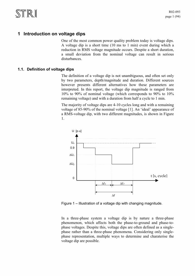
The majority of voltage dips are 4-10 cycles long and with a remaining voltage of 85-90% of the nominal voltage [1]. An ‘ideal’ appearance of a RMS-voltage dip, with two different magnitudes, is shown in Figure 1.

t [s, cycle]

U [p.u]

Un 0.9

∆U1

∆U2

0 ∆t2 ∆t1

∆t

Figure 1 – Illustration of a voltage dip with changing magnitude.

In a three-phase system a voltage dip is by nature a three-phase phenomenon, which affects both the phase-to-ground and phase-to-phase voltages. Despite this, voltage dips are often defined as a single-phase rather than a three-phase phenomena. Considering only single-phase representation, multiple ways to determine and charaterise the voltage dip are possible.

R02-093 page 2 (94)

1.1.1 The IEEE Std. 1159 definitions ” 3.1.51 sag: A decrease to between 0.1 and 0.9 p.u. in rms voltage or current at the power frequency for durations of 0.5 cycle to 1 min. Typical values are 0.1 to 0.9 p.u.”

NOTE To give a numerical value to a sag, the recommended usage is “a sag to 20%,” of which means that the line voltage is reduced down to 20% of the normal value, not reduced by 20%. Using the preposition “of” (as in “a sag of 20%,”or implied by “a 20% dip”) is deprecated.

” 3.1.73 voltage variation, short duration: A variation of the rms value of the voltage from nominal voltage for a time greater than 0.5 cycles of the power frequency but less than or equal to 1 minute. Usually further described using a modifier indicating the magnitude of a voltage variation (e.g. sag, swell, or interruption) and possibly a modifier indicating the duration of the variation (e.g., instantaneous, momentary, or temporary).” [S5]

1.1.2 The IEC 61000-2-8 definitions “2.1 voltage dip, voltage sag a sudden reduction of the voltage at a particular point on an electricity supply system below a specified dip threshold followed by its recovery after a brief interval Notes. 1 — Typically a dip is associated with the occurrence and termination of a short circuit or other extreme current increase on the system or installations connected to it. 2 — A voltage dip is a two dimensional electromagnetic disturbance, the level of which is determined by both voltage and time (duration).” “2.3 (voltage dip) reference voltage <measurement of voltage dips and short interruptions> a value specified as the base on which depth, thresholds and other values are expressed in per unit or percentage terms Note – The nominal or declared voltage of the supply system is frequently selected as the reference voltage.” “2.4 voltage dip start threshold <voltage dip measurement> an r.m.s. value of the voltage on an electricity supply system specified for the purpose of defining the start of a voltage dip Note – Typically values between 0,85 and 0,95 of the reference voltage have been used for this threshold.” “2.5 voltage dip end threshold <voltage dip measurement> an r.m.s. value of the specified for the purpose of defining the end of a voltage Note – Typically, the value used for the end threshold or has exceeded it by 0,01 of the reference voltage”. “2.9 duration (of voltage dip) the time between the instant at which the voltage at a particular point on an electricity supply system falls below

R02-093 page 3 (94)

the start threshold and the instant at which it rises to the end threshold. Note – In polyphase events, practice varies in regard to relating the start and end of the dip to the phases concerned. Future practice is likely to be that for polyphase events a dip begins when the voltage of at least one phase falls below the dip start threshold and ends when the voltage on all phases is equal to or above the dip end threshold.” “2.10 (voltage dip) sliding reference voltage <measurement of voltage dips and short interruptions> an r.m.s. value of the voltage at a particular point on an electricity supply system continuously calculated over a specified interval to represent the value of the voltage immediately preceding a voltage dip for use as the reference voltage Note – The specified interval is much longer than the duration of a voltage dip.” [S13]

1.2. Characterisation of a voltage dip The voltage during a voltage dip is often described with a constant RMS value, usually the lowest phase voltage. This is however only an approximation and often sufficient enough. In reality the RMS value varies during the voltage dip.

One approach to define a voltage level during a voltage dip, is to choose the phase with the lowest voltage and ignore the others. This method will only report one voltage dip per fault and does not distinguish between single-phase and multiple-phase voltage dips.

Another method is to consider the voltage in each phase. A voltage dip in each phase, will be counted as a separate event. With this method a three-phase-voltage dip will be counted as three voltage dips.

The third representation is to use the average voltage of all phases. This method only reports one voltage dip per fault, and usually none of the phases has the same voltage as the average.

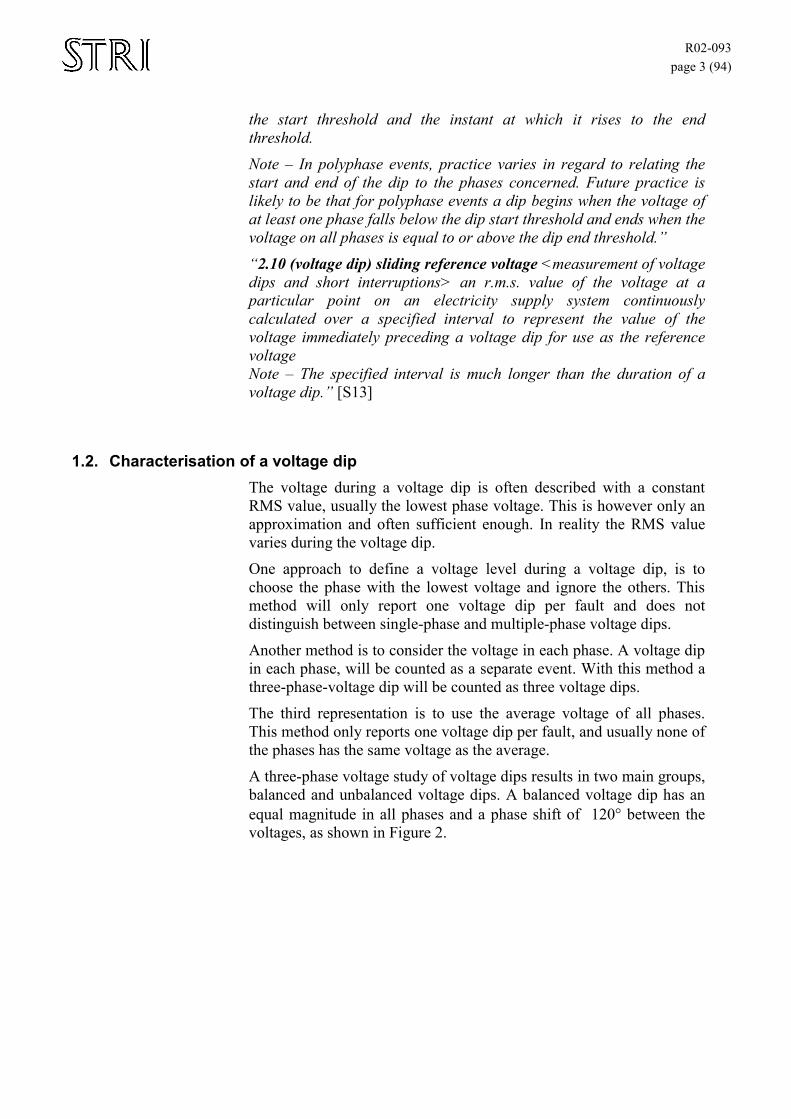
A three-phase voltage study of voltage dips results in two main groups, balanced and unbalanced voltage dips. A balanced voltage dip has an equal magnitude in all phases and a phase shift of 120° between the voltages, as shown in Figure 2.

R02-093 page 4 (94)

0 0.2 0.4 0.6 0.8 1 1.2 1.4 1.6 1.8 2 -1

-0.8

-0.6

-0.4

-0.2

0

0.2

0.4

0.6

0.8

1

A balanced three-phase voltage dip

time

volta

ge

Figure 2 – A balanced 3-phase voltage dip.

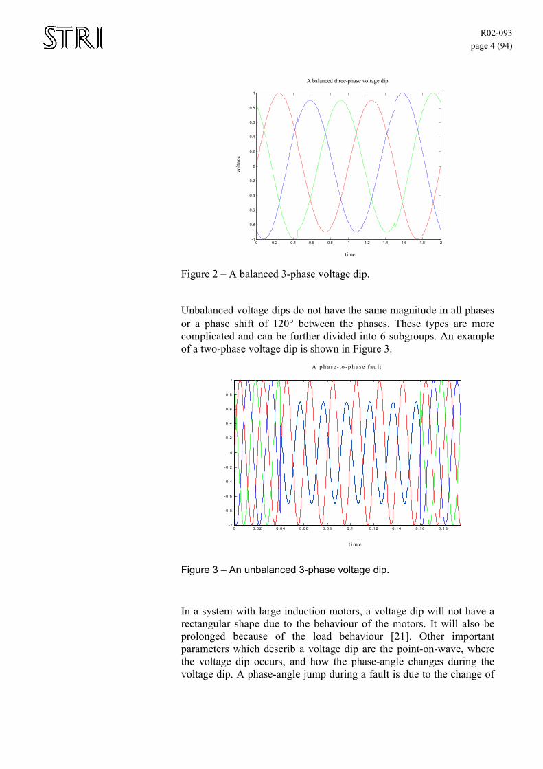
Unbalanced voltage dips do not have the same magnitude in all phases or a phase shift of 120° between the phases. These types are more complicated and can be further divided into 6 subgroups. An example of a two-phase voltage dip is shown in Figure 3.

0 0 .0 2 0 .0 4 0 .0 6 0 .0 8 0 .1 0 .1 2 0 .1 4 0 .1 6 0 .1 8 -1 -0 .8 -0 .6 -0 .4 -0 .2

0 0 .2 0 .4 0 .6 0 .8

1

tim e

A p h a se -to -p h ase fau lt

Figure 3 – An unbalanced 3-phase voltage dip.

In a system with large induction motors, a voltage dip will not have a rectangular shape due to the behaviour of the motors. It will also be prolonged because of the load behaviour [21]. Other important parameters which describ a voltage dip are the point-on-wave, where the voltage dip occurs, and how the phase-angle changes during the voltage dip. A phase-angle jump during a fault is due to the change of

R02-093 page 5 (94)

the X/R-ratio. The phase-angle-jump is a problem especially for power electronics using phase or zero-crossing switching.

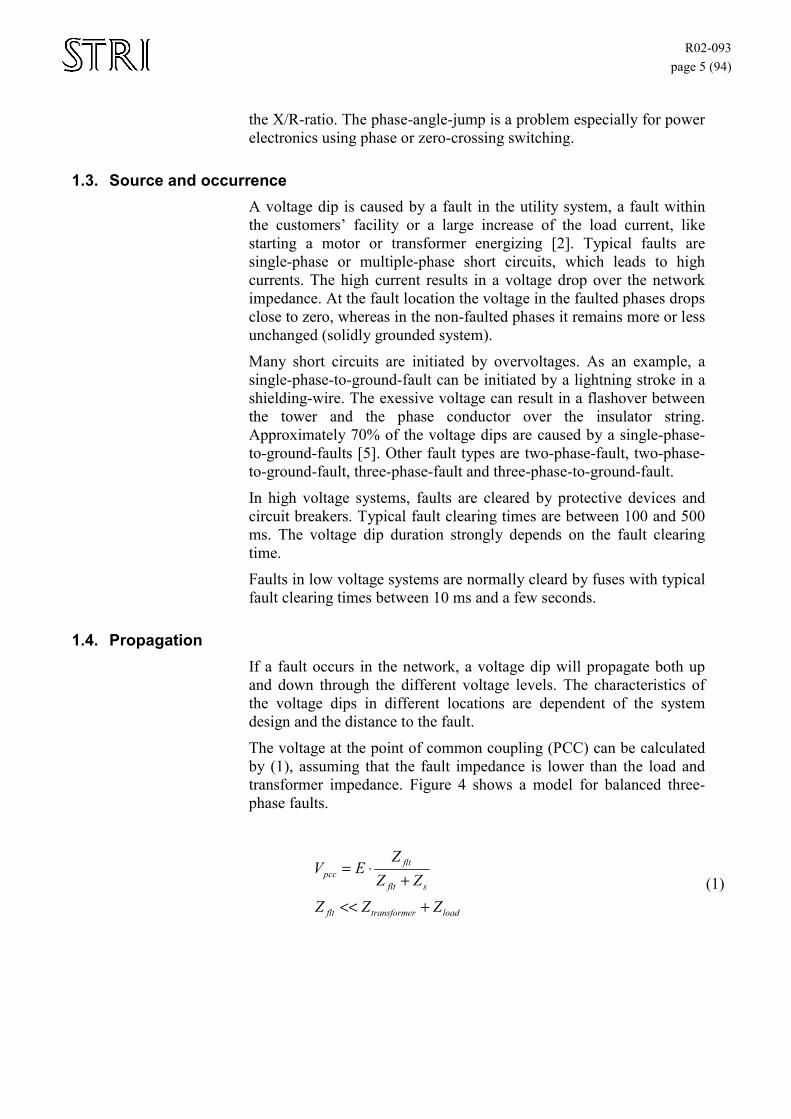
1.3. Source and occurrence A voltage dip is caused by a fault in the utility system, a fault within the customers’ facility or a large increase of the load current, like starting a motor or transformer energizing [2]. Typical faults are single-phase or multiple-phase short circuits, which leads to high currents. The high current results in a voltage drop over the network impedance. At the fault location the voltage in the faulted phases drops close to zero, whereas in the non-faulted phases it remains more or less unchanged (solidly grounded system).

Many short circuits are initiated by overvoltages. As an example, a single-phase-to-ground-fault can be initiated by a lightning stroke in a shielding-wire. The exessive voltage can result in a flashover between the tower and the phase conductor over the insulator string. Approximately 70% of the voltage dips are caused by a single-phase-to-ground-faults [5]. Other fault types are two-phase-fault, two-phase-to-ground-fault, three-phase-fault and three-phase-to-ground-fault.

In high voltage systems, faults are cleared by protective devices and circuit breakers. Typical fault clearing times are between 100 and 500 ms. The voltage dip duration strongly depends on the fault clearing time.

Faults in low voltage systems are normally cleard by fuses with typical fault clearing times between 10 ms and a few seconds.

1.4. Propagation If a fault occurs in the network, a voltage dip will propagate both up and down through the different voltage levels. The characteristics of the voltage dips in different locations are dependent of the system design and the distance to the fault.

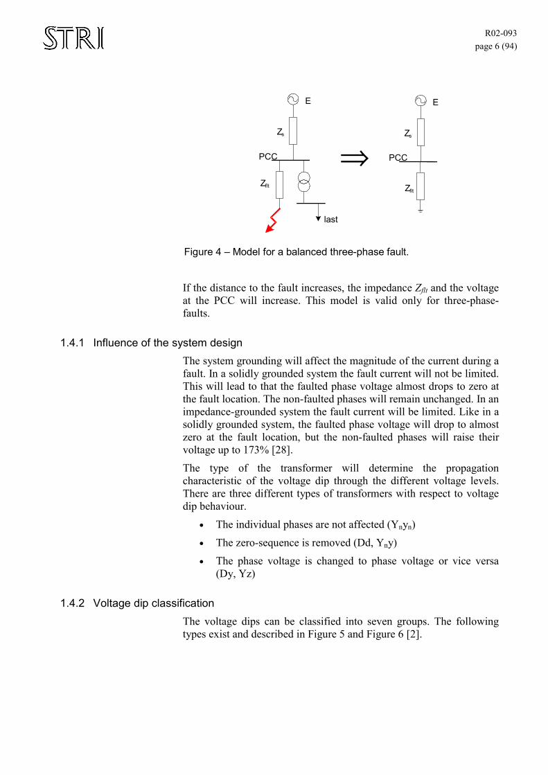
The voltage at the point of common coupling (PCC) can be calculated by (1), assuming that the fault impedance is lower than the load and transformer impedance. Figure 4 shows a model for balanced three-phase faults.

loadrtransformeflt

sflt

fltpcc

ZZZZZ

ZEV

+<<

+⋅=

(1)

R02-093 page 6 (94)

Z flt

Z s

E

Z s

last

E

PCC PCC ⇒

Z flt

Figure 4 – Model for a balanced three-phase fault.

If the distance to the fault increases, the impedance Zflt and the voltage at the PCC will increase. This model is valid only for three-phase-faults.

1.4.1 Influence of the system design The system grounding will affect the magnitude of the current during a fault. In a solidly grounded system the fault current will not be limited. This will lead to that the faulted phase voltage almost drops to zero at the fault location. The non-faulted phases will remain unchanged. In an impedance-grounded system the fault current will be limited. Like in a solidly grounded system, the faulted phase voltage will drop to almost zero at the fault location, but the non-faulted phases will raise their voltage up to 173% [28].

The type of the transformer will determine the propagation characteristic of the voltage dip through the different voltage levels. There are three different types of transformers with respect to voltage dip behaviour.

• The individual phases are not affected (Ynyn)

• The zero-sequence is removed (Dd, Yny)

• The phase voltage is changed to phase voltage or vice versa (Dy, Yz)

1.4.2 Voltage dip classification The voltage dips can be classified into seven groups. The following types exist and described in Figure 5 and Figure 6 [2].

R02-093 page 7 (94)

Type A Type B

Type C Type D

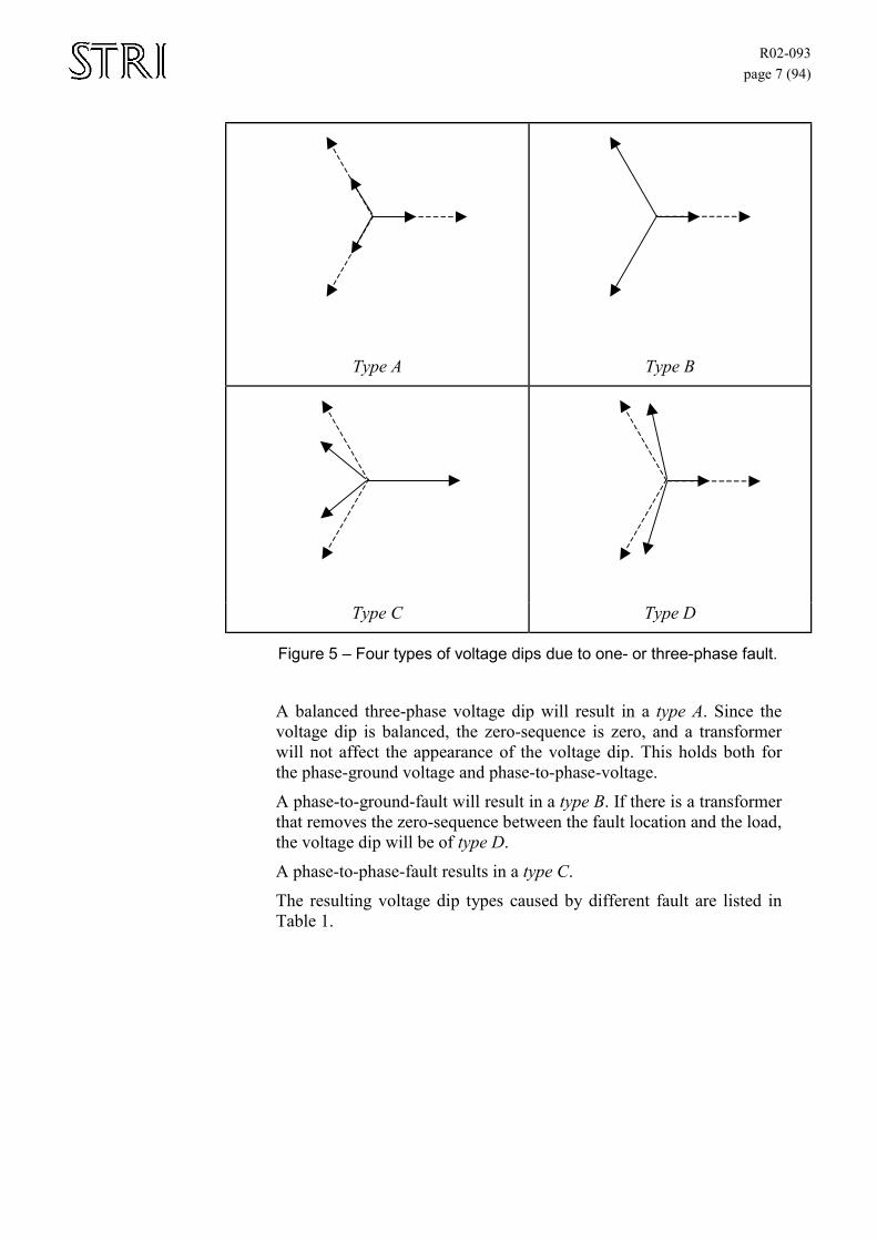
Figure 5 – Four types of voltage dips due to one- or three-phase fault.

A balanced three-phase voltage dip will result in a type A. Since the voltage dip is balanced, the zero-sequence is zero, and a transformer will not affect the appearance of the voltage dip. This holds both for the phase-ground voltage and phase-to-phase-voltage.

A phase-to-ground-fault will result in a type B. If there is a transformer that removes the zero-sequence between the fault location and the load, the voltage dip will be of type D.

A phase-to-phase-fault results in a type C.

The resulting voltage dip types caused by different fault are listed in Table 1.

R02-093 page 8 (94)

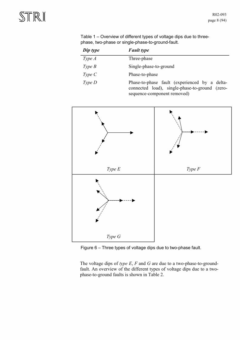
Table 1 – Overview of different types of voltage dips due to three-phase, two-phase or single-phase-to-ground-fault.

Dip type Fault type

Type A Three-phase

Type B Single-phase-to-ground

Type C Phase-to-phase

Type D Phase-to-phase fault (experienced by a delta-connected load), single-phase-to-ground (zero-sequence-component removed)

Type E Type F

Type G

Figure 6 – Three types of voltage dips due to two-phase fault.

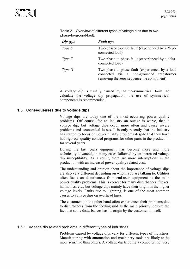
The voltage dips of type E, F and G are due to a two-phase-to-ground-fault. An overview of the different types of voltage dips due to a two-phase-to-ground faults is shown in Table 2.

R02-093 page 9 (94)

Table 2 – Overview of different types of voltage dips due to two-phase-to-ground-fault.

Dip type Fault type

Type E Two-phase-to-phase fault (experienced by a Wye-connected load)

Type F Two-phase-to-phase fault (experienced by a delta-connected load)

Type G Two-phase-to-phase fault (experienced by a load connected via a non-grounded transformer removing the zero-sequence the component)

A voltage dip is usually caused by an un-symmetrical fault. To calculate the voltage dip propagation, the use of symmetrical components is recommended.

1.5. Consequenses due to voltage dips Voltage dips are today one of the most occurring power quality problems. Off course, for an industry an outage is worse, than a voltage dip, but voltage dips occur more often and cause severe problems and economical losses. It is only recently that the industry has started to focus on power quality problems despite that they have had rigorous quality control programs for other parts in the production for several years.

During the last years equipment has become more and more technically advanced, in many cases followed by an increased voltage dip susceptibility. As a result, there are more interruptions in the production with an increased power quality related cost.

The understanding and opinion about the importance of voltage dips are also very different depending on whom you are talking to. Utilities often focus on disturbances from end-user equipment as the main power quality problems. This is correct for many disturbances, flicker, harmonics, etc., but voltage dips mainly have their origin in the higher voltage levels. Faults due to lightning, is one of the most common causes to voltage dips on overhead lines.

The customers on the other hand often experiences their problems due to disturbances from the feeding grid as the main priority, despite the fact that some disturbances has its origin by the customer himself.

1.5.1 Voltage dip related problems in different types of industries Problems caused by voltage dips vary for different types of industries. Manufacturing with automation and machinery tools are likely to be more sensitive than others. A voltage dip tripping a computer, not very

R02-093 page 10 (94)

often causes more than one hour of interruption and a restart takes only a couple of minutes [28]. However, there are some exceptions e.g. stock market, banks, etc., where an interruption can be very expensive.

A large plant or process can need as long time as a week to restart and there can be weeks before the quality requirement of the production has reached the normal levels. There is often some loss in production due to the voltage dip and in some cases the products in the process have to be discarded.

There are also large differences in costs depending on if the voltage dip leads to a controlled shutdown or if there are damages caused by it.

1.5.1.1 Offices A voltage dip is normally not a huge problem to single computers unless they are used as servers or mainframe computers. In such cases it is relatively easy to protect them, for a minor cost, by using UPS.

The problem is not very significant to ordinary single PC’s since the lost work not often exceeds 1-2 hour’s work and often there is a backup or automatic restore of the file [28]. However there are some PC-based offices where a disruption will cost greatly. Financial trading and telecommunication offices are typical examples. In financial trading a disruption can cost as much as € 6 Million per hour and for a telecommunication station € 1.8 Million per hour [31]. In both cases there is a high awareness to power quality and sophisticated backup systems are often used to make these applications withstand voltage dips.

1.5.1.2 Pulp and Paper industry A pulp and paper mill is a very complex plant and has therefore very often a varying immunity level. A disturbance in the process can lead to two different faults; a total shut-down or a partial disturbance. Unfortunately the buffer stocks between different sub-processes are often very low and the processes strongly depend on each other. This can lead to a situation where a small process is shutdown, but since the buffer can run out for other processes, they also have to stop.

Another common situation in pulp and paper mills is that 70 % of the electrical energy is used in different kind of motors [10]. This will affect the voltage dip, prolonging and smoothen it, and may cause additional stops. The restart after a complete stop of a pulp and paper mill takes approximately 10 hours up to 5 days and for a pure paper mill around 5-20 hours. Even if the production has started, very often the quality of the pulp and paper are degraded immediately after the restart [19].

1.5.1.3 Semiconductor industry The semiconductor sector is one of the most sensitive sectors of all industries [12]. It is also one of few which is working very actively

R02-093 page 11 (94)

with the problem. In the semiconductor industry there are several types of advanced machines with different immunity levels against voltage dips. The semiconductor organisation, SEMI, has specified operational conditions for equipment during voltage dips, which requires new equipment to be better than many of the old [SEMI F47]. Nevertheless voltage dips are still a problem. Many machines in a semiconductor factory contain high precision drives and control circuits, and are therefore very sensitive. Another vast number of equipment in the industry is the testing, packaging and welding machines, which are all controlled by some sort of computer. A disturbance large enough can cause these machines to malfunction. After a dropout a few of them can automatically restart but the rest have to be manually restarted. The restart procedure is in some cases very time-consuming if there are many machines and few personel e.g. during night.

1.5.1.4 Pharmaceutical The production in pharmaceutical industry is often conducted in batches and therefore a disturbance in one process can, in a worst-case scenario, lead to a discard of a whole batch. The discard decision of a batch can either be based on a true fault e.g. a pump, a boiler, a separator or other equipment has malfunctioned, or the sensors can have given a false signal due to the voltage dip. Typical equipment in plants are pumps, boilers, autoclaves, control devices, etc. All of the equipment can be very sensitive to disturbances since they are very complex and requires precise operation. There have been published very few studies from pharmaceutical industries in technical papers but the assumption that they will have the same experience as other industries with similar equipment is logical.

1.5.1.5 Steel mill A mill producing steel products has a lot of large adjustable speed drives and synchronous machines in the process. The machines, especially the synchronous motors, are large powered and can therefore stop fast during a voltage dip. The risk is higher if they are in a full load situation e.g. rolling phase. A long restarting time is the main problem for a steel mill. It can take several hours to start-up the process after an unplanned stop caused by a voltage dip. There is also a risk of permanent damage due to a stop, depending on where in the rolling process the interruption occurs. In an unfortunate stage, the hot steel slab is between two rolls and these may be deformed. Since it is impossible to cool the contact area an unplanned stop is very critical [18].

1.5.1.6 Other industries There are a lot of industries suffering from voltage dips. Some are more ‘advanced’ and specialized than others. Example of other industries which can have problems related to voltage dips are oil

R02-093 page 12 (94)

refineries, textile industries, industries with conveyor belts and industries with a high level of automation and control.

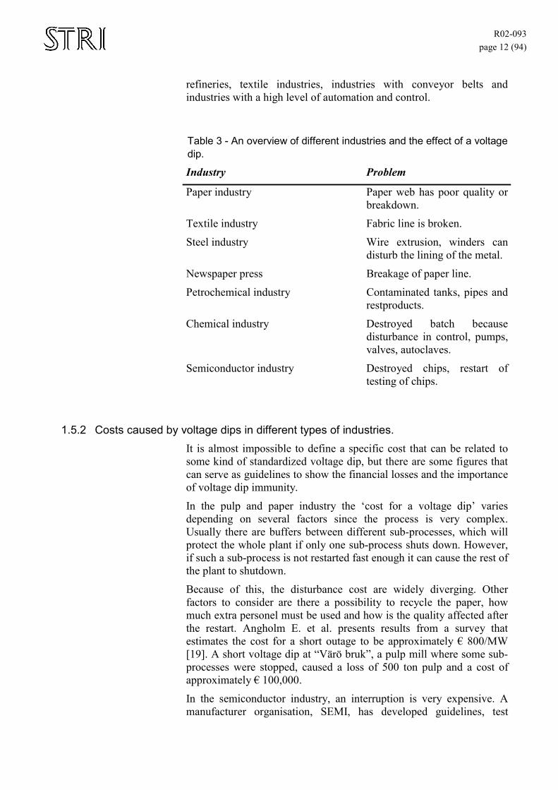
Table 3 - An overview of different industries and the effect of a voltage dip.

Industry Problem

Paper industry Paper web has poor quality or breakdown.

Textile industry Fabric line is broken.

Steel industry Wire extrusion, winders can disturb the lining of the metal.

Newspaper press Breakage of paper line.

Petrochemical industry Contaminated tanks, pipes and restproducts.

Chemical industry Destroyed batch because disturbance in control, pumps, valves, autoclaves.

Semiconductor industry Destroyed chips, restart of testing of chips.

1.5.2 Costs caused by voltage dips in different types of industries. It is almost impossible to define a specific cost that can be related to some kind of standardized voltage dip, but there are some figures that can serve as guidelines to show the financial losses and the importance of voltage dip immunity.

In the pulp and paper industry the ‘cost for a voltage dip’ varies depending on several factors since the process is very complex. Usually there are buffers between different sub-processes, which will protect the whole plant if only one sub-process shuts down. However, if such a sub-process is not restarted fast enough it can cause the rest of the plant to shutdown.

Because of this, the disturbance cost are widely diverging. Other factors to consider are there a possibility to recycle the paper, how much extra personel must be used and how is the quality affected after the restart. Angholm E. et al. presents results from a survey that estimates the cost for a short outage to be approximately € 800/MW [19]. A short voltage dip at “Värö bruk”, a pulp mill where some sub-processes were stopped, caused a loss of 500 ton pulp and a cost of approximately € 100,000.

In the semiconductor industry, an interruption is very expensive. A manufacturer organisation, SEMI, has developed guidelines, test

R02-093 page 13 (94)

procedure and limits for voltage dip susceptibility for different types of equipment used in their factories. The semiconductor industry in Taiwan has estimated their losses to € 1.7 million per voltage dip [26].

In the plastic extrusion industry, adjustable speed drives (ASD) are used to produce plastic bags, carpet fibres etc. The extrusion process is completely automated using ASD. A short voltage dip can strike out one or more ASD’s. An uncontrolled shutdown can damage the equipment, result in unusable products, need of cleaning the machines and degrated quality of products. All disturbances are very expensive, the losses are in order of € 10,000 per event and 20-25 events occurs annually [14].

Another cost-sensitive category of industries, with respect to voltage dips, are the steel industry, shown by an investigation made at Oxelösund, Sweden [18]. A hot rolling mill driven by two synchronous machines at 11.2 MW each have production losses in the mill which are estimated to € 100,000 per hour.

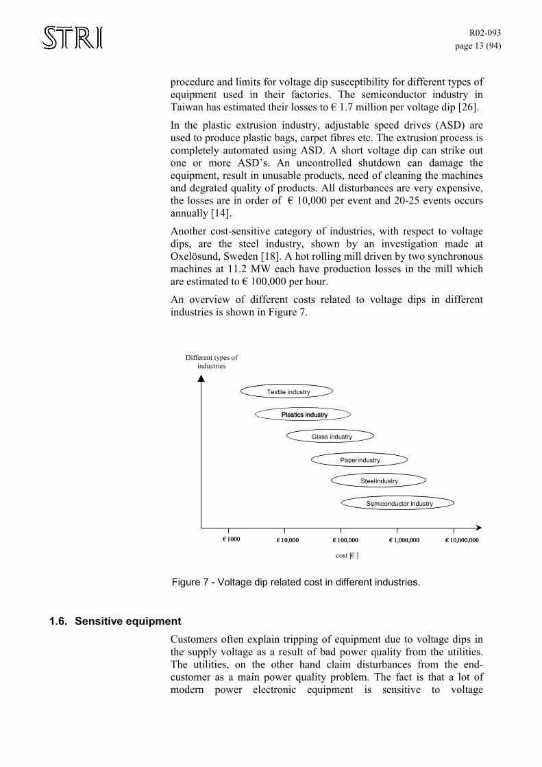
An overview of different costs related to voltage dips in different industries is shown in Figure 7.

€ 1000 € 10,000 € 100,000 € 1,000,000 € 10,000,000

Textile industry

Plastics industry

Glass industry

Semiconductor industry

Steel industry

Paperindustry

€ 1000 € 10,000 € 100,000 € 1,000,000 € 10,000,000

Textile industry

Plastics industry

Glass industry

Semiconductor industry

Steel industry

Paperindustry

Different types of industries

cost [€ ]

Figure 7 - Voltage dip related cost in different industries.

1.6. Sensitive equipment Customers often explain tripping of equipment due to voltage dips in the supply voltage as a result of bad power quality from the utilities. The utilities, on the other hand claim disturbances from the end-customer as a main power quality problem. The fact is that a lot of modern power electronic equipment is sensitive to voltage

R02-093 page 14 (94)

disturbances and it has been confirmed that this equipment causes disturbances for other customers as well as to themselves. Unfortunately, equipment susceptibility has become worse compared to its counterparts 10 or 20 years ago [12].

The increased use of converter-driven equipment, non-linear consumer electronics and computers, has led to a large growth of voltage disturbances in the systems.

Different components are often combined into systems and shall therefore be considered as a system, rather than a number of single components. This makes the analysis and determination of the system susceptibility difficult. A study of each component in a system is much easier, and can give a hint of the overall system behaviour and weak spots.

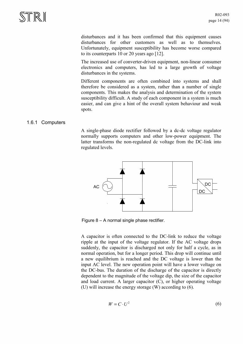
1.6.1 Computers A single-phase diode rectifier followed by a dc-dc voltage regulator normally supports computers and other low-power equipment. The latter transforms the non-regulated dc voltage from the DC-link into regulated levels.

DCDCAC

Figure 8 – A normal single phase rectifier.

A capacitor is often connected to the DC-link to reduce the voltage ripple at the input of the voltage regulator. If the AC voltage drops suddenly, the capacitor is discharged not only for half a cycle, as in normal operation, but for a longer period. This drop will continue until a new equilibrium is reached and the DC voltage is lower than the input AC level. The new operation point will have a lower voltage on the DC-bus. The duration of the discharge of the capacitor is directly dependent to the magnitude of the voltage dip, the size of the capacitor and load current. A larger capacitor (C), or higher operating voltage (U) will increase the energy storage (W) according to (6).

2UCW ⋅= (6)

R02-093 page 15 (94)

The voltage regulator is often able to maintain the output voltage level for some variations in the input voltage, but at too low levels the over current protection will trip. The purpose of a trip is to protect the components on the other side of the regulator. In some configurations the rectifier also has under-voltage protection on the AC-side, which may trip during a voltage dip. The purpose of the AC-side under-voltage protection is to limit the current to the circuit.

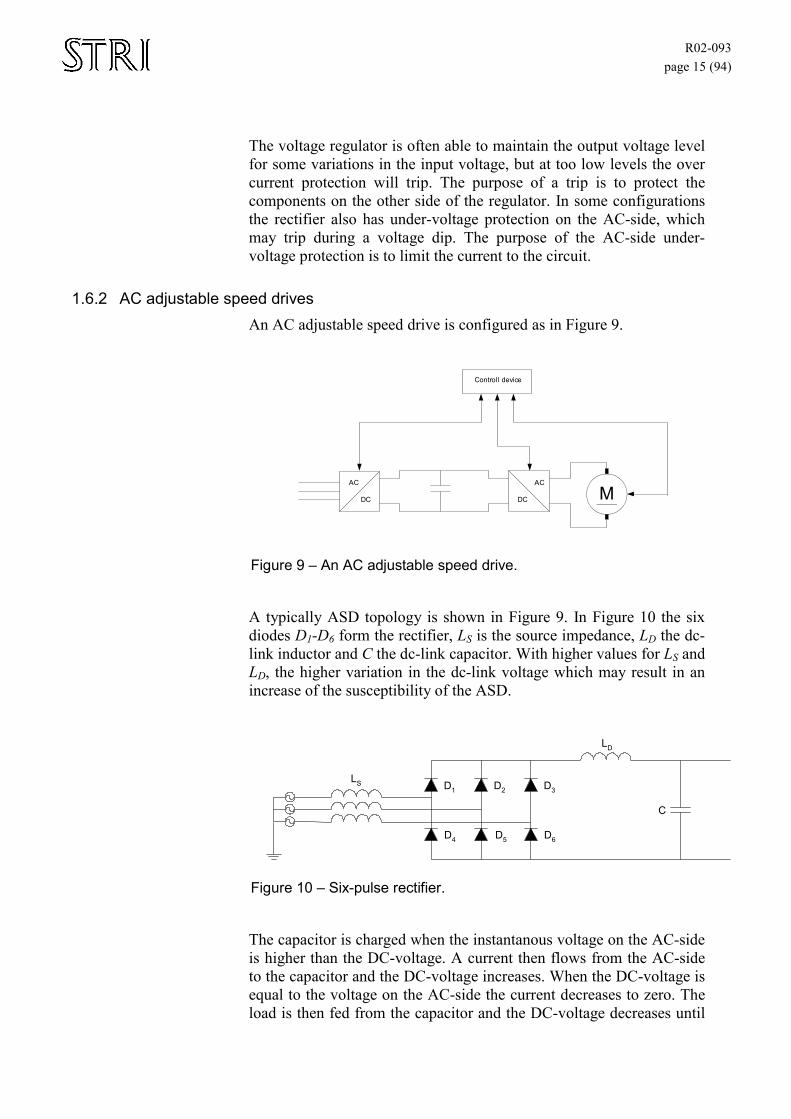
1.6.2 AC adjustable speed drives An AC adjustable speed drive is configured as in Figure 9.

MDC

AC

DC

AC

Controll device

Figure 9 – An AC adjustable speed drive.

A typically ASD topology is shown in Figure 9. In Figure 10 the six diodes D1-D6 form the rectifier, LS is the source impedance, LD the dc-link inductor and C the dc-link capacitor. With higher values for LS and LD, the higher variation in the dc-link voltage which may result in an increase of the susceptibility of the ASD.

D6

D1 D2 D3

D4 D5

LD

C

LS

Figure 10 – Six-pulse rectifier.

The capacitor is charged when the instantanous voltage on the AC-side is higher than the DC-voltage. A current then flows from the AC-side to the capacitor and the DC-voltage increases. When the DC-voltage is equal to the voltage on the AC-side the current decreases to zero. The load is then fed from the capacitor and the DC-voltage decreases until

R02-093 page 16 (94)

the AC-side voltage is greater than the remaining DC-voltage. In steady-state there are six current pulses on the DC-side per cycle.

During a voltage dip the voltage on the AC-side is reduced. Depending on type and duration of the voltage dip, the voltage on the DC-side may change. A voltage dip of type A (balanced three-phase) will result in a reduction of the voltage on the DC-side proportional to the AC-side. This type of voltage dip is normally the most severe. The under-voltage or over current-protection on the DC-side may trip the ASD.

If the voltage dip is of type C, the circuit will behave as a single-phase rectifier. A 10% voltage dip will result in a single-phase operation of the three-phase diode rectifier [20]. The voltage between the two non-faulted phases is un-affected and the DC-side voltage will not be reduced. The current pulses will however be changed. The same amount of energy must be transferred, but now in two pulses instead of six. The peak value of the current will be 200% larger, and may cause an over-current or a current unbalance. The over-current or unbalance protection may trip the ASD. A phase-angle-jump will affect the phase voltages. It will affect the DC-link voltage [28].

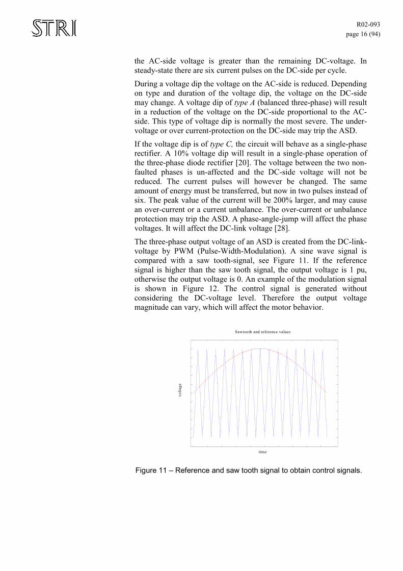
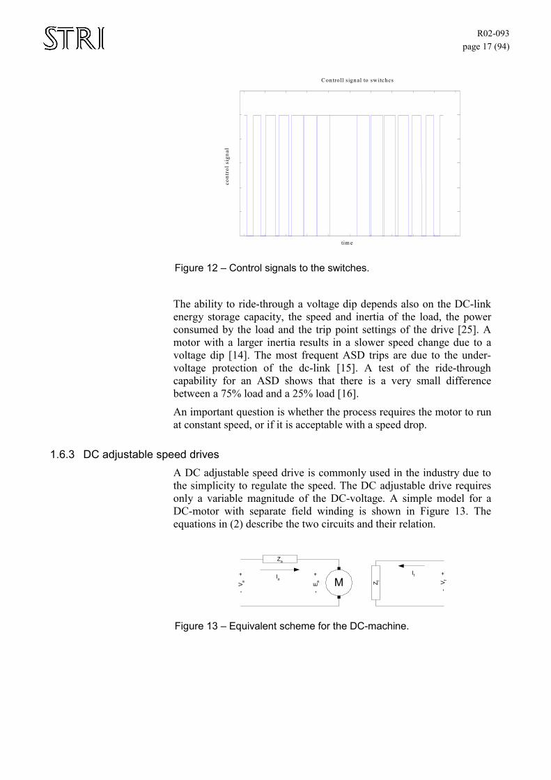
The three-phase output voltage of an ASD is created from the DC-link-voltage by PWM (Pulse-Width-Modulation). A sine wave signal is compared with a saw tooth-signal, see Figure 11. If the reference signal is higher than the saw tooth signal, the output voltage is 1 pu, otherwise the output voltage is 0. An example of the modulation signal is shown in Figure 12. The control signal is generated without considering the DC-voltage level. Therefore the output voltage magnitude can vary, which will affect the motor behavior.

time

Sawtooth and reference values

volta

ge

Figure 11 – Reference and saw tooth signal to obtain control signals.

R02-093 page 17 (94)

tim e

C ontro ll signal to sw itches

cont

rol s

igna

l

Figure 12 – Control signals to the switches.

The ability to ride-through a voltage dip depends also on the DC-link energy storage capacity, the speed and inertia of the load, the power consumed by the load and the trip point settings of the drive [25]. A motor with a larger inertia results in a slower speed change due to a voltage dip [14]. The most frequent ASD trips are due to the under-voltage protection of the dc-link [15]. A test of the ride-through capability for an ASD shows that there is a very small difference between a 75% load and a 25% load [16].

An important question is whether the process requires the motor to run at constant speed, or if it is acceptable with a speed drop.

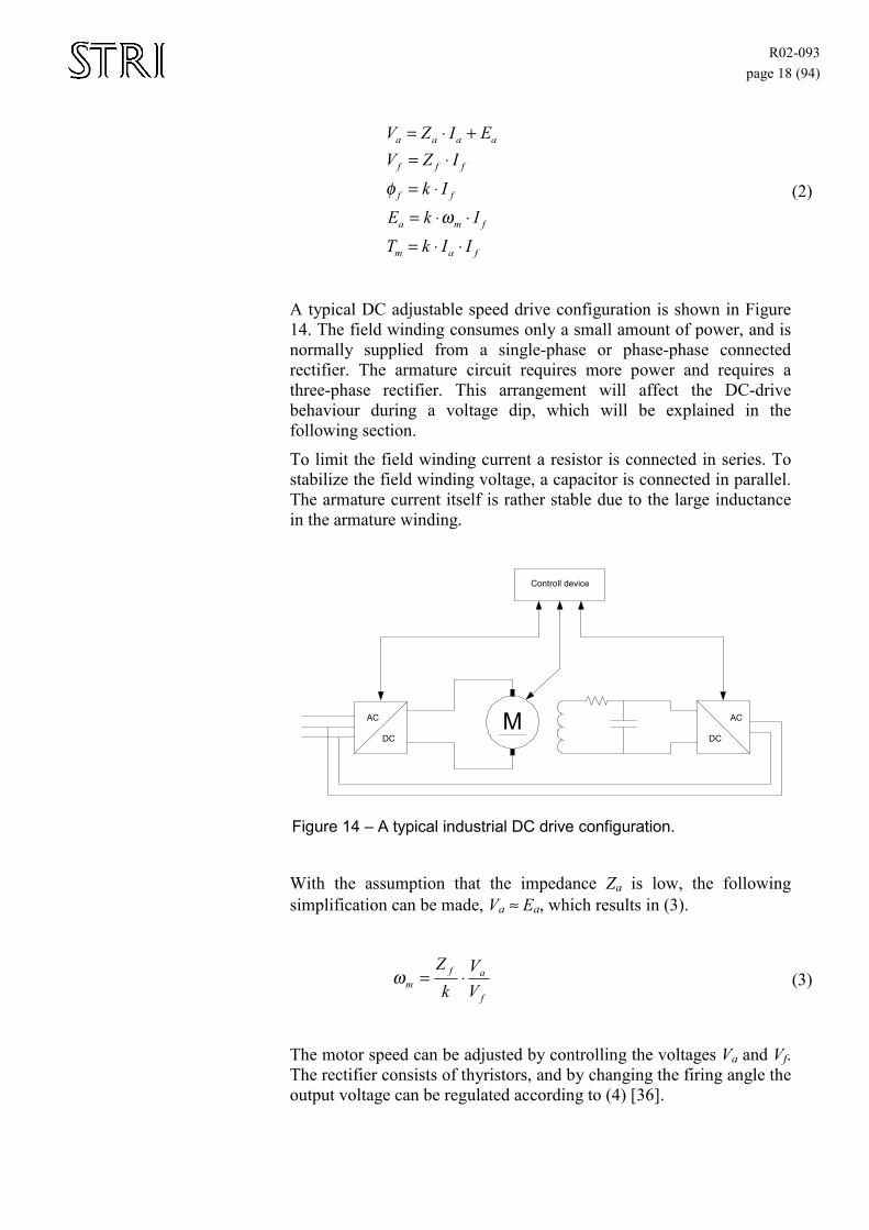
1.6.3 DC adjustable speed drives A DC adjustable speed drive is commonly used in the industry due to the simplicity to regulate the speed. The DC adjustable drive requires only a variable magnitude of the DC-voltage. A simple model for a DC-motor with separate field winding is shown in Figure 13. The equations in (2) describe the two circuits and their relation.

M

Za

Z f

- E

a +

- V

a +

- V

f +Ia

If

Figure 13 – Equivalent scheme for the DC-machine.

R02-093 page 18 (94)

fam

fma

ff

fff

aaaa

IIkTIkE

IkIZV

EIZV

⋅⋅=

⋅⋅=

⋅=

⋅=+⋅=

ωφ (2)

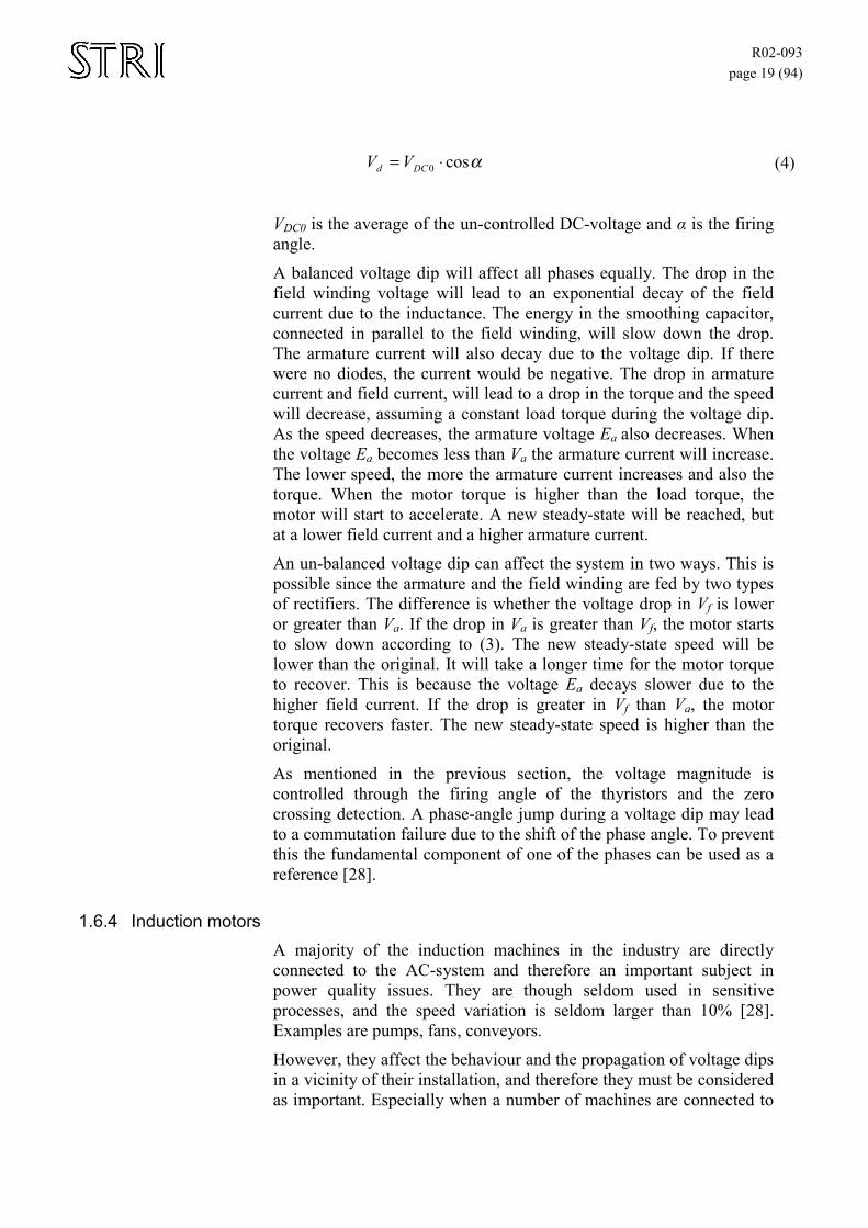
A typical DC adjustable speed drive configuration is shown in Figure 14. The field winding consumes only a small amount of power, and is normally supplied from a single-phase or phase-phase connected rectifier. The armature circuit requires more power and requires a three-phase rectifier. This arrangement will affect the DC-drive behaviour during a voltage dip, which will be explained in the following section.

To limit the field winding current a resistor is connected in series. To stabilize the field winding voltage, a capacitor is connected in parallel. The armature current itself is rather stable due to the large inductance in the armature winding.

MDC

AC

DC

AC

Controll device

Figure 14 – A typical industrial DC drive configuration.

With the assumption that the impedance Za is low, the following simplification can be made, Va ≈ Ea, which results in (3).

f

afm V

Vk

Z⋅=ω (3)

The motor speed can be adjusted by controlling the voltages Va and Vf. The rectifier consists of thyristors, and by changing the firing angle the output voltage can be regulated according to (4) [36].

R02-093 page 19 (94)

αcos0 ⋅= DCd VV (4)

VDC0 is the average of the un-controlled DC-voltage and α is the firing angle.

A balanced voltage dip will affect all phases equally. The drop in the field winding voltage will lead to an exponential decay of the field current due to the inductance. The energy in the smoothing capacitor, connected in parallel to the field winding, will slow down the drop. The armature current will also decay due to the voltage dip. If there were no diodes, the current would be negative. The drop in armature current and field current, will lead to a drop in the torque and the speed will decrease, assuming a constant load torque during the voltage dip. As the speed decreases, the armature voltage Ea also decreases. When the voltage Ea becomes less than Va the armature current will increase. The lower speed, the more the armature current increases and also the torque. When the motor torque is higher than the load torque, the motor will start to accelerate. A new steady-state will be reached, but at a lower field current and a higher armature current.

An un-balanced voltage dip can affect the system in two ways. This is possible since the armature and the field winding are fed by two types of rectifiers. The difference is whether the voltage drop in Vf is lower or greater than Va. If the drop in Va is greater than Vf, the motor starts to slow down according to (3). The new steady-state speed will be lower than the original. It will take a longer time for the motor torque to recover. This is because the voltage Ea decays slower due to the higher field current. If the drop is greater in Vf than Va, the motor torque recovers faster. The new steady-state speed is higher than the original.

As mentioned in the previous section, the voltage magnitude is controlled through the firing angle of the thyristors and the zero crossing detection. A phase-angle jump during a voltage dip may lead to a commutation failure due to the shift of the phase angle. To prevent this the fundamental component of one of the phases can be used as a reference [28].

1.6.4 Induction motors A majority of the induction machines in the industry are directly connected to the AC-system and therefore an important subject in power quality issues. They are though seldom used in sensitive processes, and the speed variation is seldom larger than 10% [28]. Examples are pumps, fans, conveyors.

However, they affect the behaviour and the propagation of voltage dips in a vicinity of their installation, and therefore they must be considered as important. Especially when a number of machines are connected to

R02-093 page 20 (94)

the same busbar the consequences of a voltage dip can be severe. The reason for this is that even a single induction machine can affect the voltage dip magnitude and duration. The result can therefore be that some of the other sensitive equipment, which are able to withstand the original voltage dip, will drop out during the post-voltage dip. This is due to the changed voltage dip characteristic by the induction motors.

Even under normal conditions, a direct start of an inductor motor will cause a voltage dip. During a normal motor start there is often a controlled procedure and therefore lower current peaks. One main problem with a voltage dip is that it may initiate torque oscillations in the beginning and in the end of the voltage reduction. This phenomenon can cause damage to the motor or interrupt the process. The recovery torque can also be much more severe if the motor flux is out of phase with the supply voltage [22].

Another problem associated with voltage dips and the induction machine is the behaviour of the machine when the voltage dip occurs. At the beginning of the voltage dip, the voltage drops and since the torque is proportional to the square of the voltage, the speed will also drop. The speed will drop further during the voltage dip, since the magnetic field in the rotor is driven out of the air gap and the associated transient causes an additional drop in speed. This is caused since the flux is in unbalance with the stator voltage and therefore the torque decreases. A positive effect is that when the flux starts to decay, the motor will contribute with energy and act as a generator. This behaviour usually mitigates the voltage dip but it also deforms the characteristics so that the voltage dip no longer is rectangular [30]. Unfortunately this leads to another problem when the voltage recovers.

The air gap field first has to be rebuilt and then the motor will start to reaccelerate. During the post-voltage dip stage the motor will draw a large inrush current, mainly to build up the air gap field but also due to reacceleration.

In most practical cases the load torque decreases and motor torque increases when the motor slows down. This mitigates the problem and makes it easier, for the motor to restart. Often the event is so fast that the torque can be considered constant and the actual speed drop is often less than expected. For some loads, with almost constant torque or large inertia, the motor will need a large current as described and for some loads the motor will not be able to restart at all.

The high current during the post-voltage dip stage can prolong the voltage dip long enough to trip the under-voltage protection. Especially in cases with a vast number of machines, or in a weak network, this problem is common. To avoid the problem the industry shall have a reaccelerating plan for a controlled start up after a sudden stop.

The response to voltage dips is different depending on the type of the voltage dip. Unbalance voltage dips of types B, C, D, E, F and G,

R02-093 page 21 (94)

usually results in a smoother behaviour of the torque and current. The unbalanced voltage dip of type B can in some cases cause higher peaks than symmetrical voltage dips [23]. However, type B is very rare, because of the transformers in the transmission and the distribution network.

A third problem related to unbalanced voltage dips is the winding and stator losses caused by the negative sequence voltage. In some cases this can result in an increased temperature [29].

Balanced voltage dips, with the same duration and depth in all phases are the worst for induction machines.

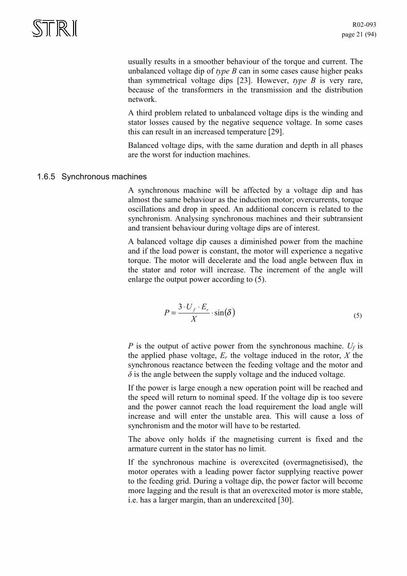
1.6.5 Synchronous machines A synchronous machine will be affected by a voltage dip and has almost the same behaviour as the induction motor; overcurrents, torque oscillations and drop in speed. An additional concern is related to the synchronism. Analysing synchronous machines and their subtransient and transient behaviour during voltage dips are of interest.

A balanced voltage dip causes a diminished power from the machine and if the load power is constant, the motor will experience a negative torque. The motor will decelerate and the load angle between flux in the stator and rotor will increase. The increment of the angle will enlarge the output power according to (5).

( )δsin3

⋅⋅⋅

=X

EUP rf (5)

P is the output of active power from the synchronous machine. Uf is the applied phase voltage, Er the voltage induced in the rotor, X the synchronous reactance between the feeding voltage and the motor and δ is the angle between the supply voltage and the induced voltage.

If the power is large enough a new operation point will be reached and the speed will return to nominal speed. If the voltage dip is too severe and the power cannot reach the load requirement the load angle will increase and will enter the unstable area. This will cause a loss of synchronism and the motor will have to be restarted.

The above only holds if the magnetising current is fixed and the armature current in the stator has no limit.

If the synchronous machine is overexcited (overmagnetisised), the motor operates with a leading power factor supplying reactive power to the feeding grid. During a voltage dip, the power factor will become more lagging and the result is that an overexcited motor is more stable, i.e. has a larger margin, than an underexcited [30].

R02-093 page 22 (94)

Another problem can occur in configurations where the magnetisation current is fed from a rectifier connected to the same source as the machine. This will result in a voltage dip in the current causing a rapid reduction in torque. As a result of this, the change in torque oscillations will be larger compared to a system with constant excitation system or permanent magnets. The current needed for excitation is often small and can therefore be supplied from a rectifier charged battery system.

In some systems the control algorithm is designed to attenuate the field current during a voltage dip, reducing the problem.

Another way of solving the problem is to use a pullout relay connected to the rotor. When the relay senses the current pulsations in the rotor it will, instead of tripping the motor from the power supply, only trip the field excitation. The machine will then behave like an asynchronous machine and slow down. Later on, when the voltage recovers, applying excitation at optimum slip and angle can easily restart the motor.

To solve the oscillation problem many synchronous machines are equipped with damping windings. These are special stator windings placed to damp the rotor oscillations.

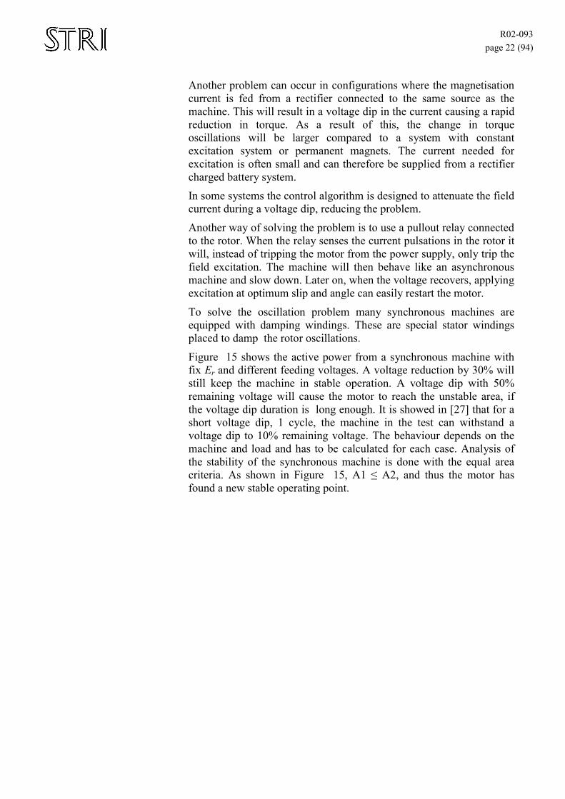
Figure 15 shows the active power from a synchronous machine with fix Er and different feeding voltages. A voltage reduction by 30% will still keep the machine in stable operation. A voltage dip with 50% remaining voltage will cause the motor to reach the unstable area, if the voltage dip duration is long enough. It is showed in [27] that for a short voltage dip, 1 cycle, the machine in the test can withstand a voltage dip to 10% remaining voltage. The behaviour depends on the machine and load and has to be calculated for each case. Analysis of the stability of the synchronous machine is done with the equal area criteria. As shown in Figure 15, A1 ≤ A2, and thus the motor has found a new stable operating point.

R02-093 page 23 (94)

0º 20º 40º 60º 80º 100º 120º 140º 160º 180º 0

0.1

0.2

0.3

0.4

0.5

0.6

0.7

0.8

0.9

1 p.u.

Load angle, δ

Motor power

Load power

100% voltage

70% voltage

50% voltage AAA111

AAA222 vo

ltage

Figure 15 – Active power in a synchronous motor as a function of the load angle for different voltages.

In many applications the synchronous machine is not directly connected to the grid. Instead it is fed via a frequency-converter. The inverter fed machine is used as e.g. compressors, fans, pumps, rolling mills. Usually rated between 1000 to 4000 kW and preferably operated at high speeds.

There is also another type of converter used in very large (several MW), slow moving systems e.g. mine, steel industry. This converter consists of three thyristor-based inverters.

The effects of voltage dips in these systems are similar to the ones above, but the voltage variations depend mainly on how the converters reacts. The behaviour of the rectifiers is described in section “AC adjustable speed drives”

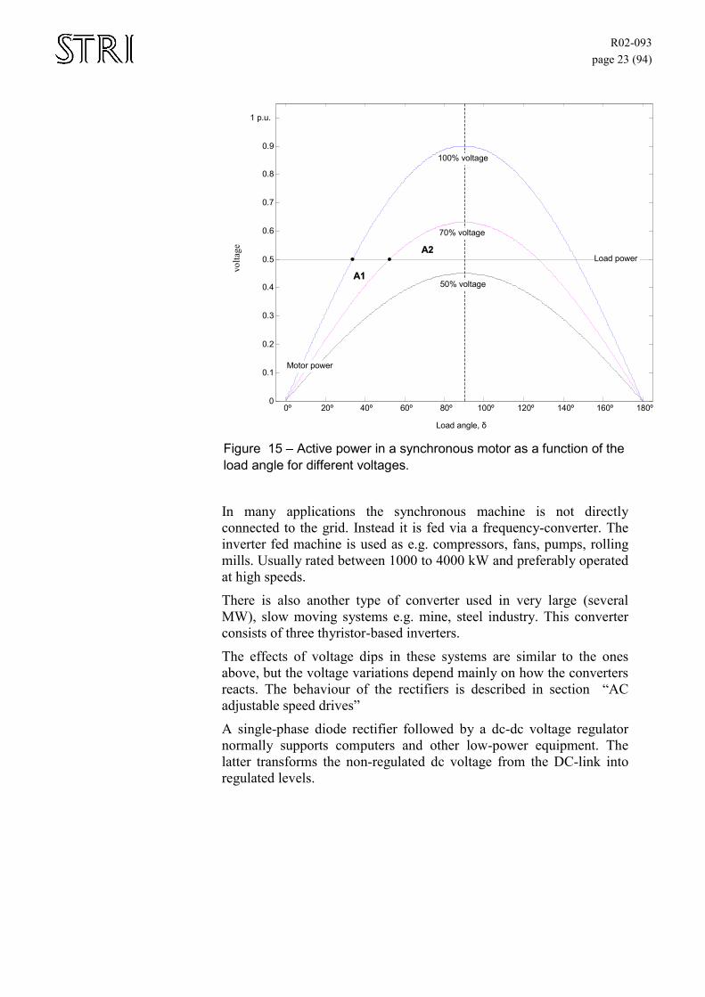
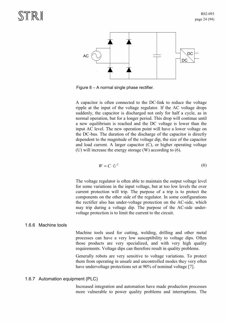
A single-phase diode rectifier followed by a dc-dc voltage regulator normally supports computers and other low-power equipment. The latter transforms the non-regulated dc voltage from the DC-link into regulated levels.

R02-093 page 24 (94)

DCDCAC

Figure 8 – A normal single phase rectifier.

A capacitor is often connected to the DC-link to reduce the voltage ripple at the input of the voltage regulator. If the AC voltage drops suddenly, the capacitor is discharged not only for half a cycle, as in normal operation, but for a longer period. This drop will continue until a new equilibrium is reached and the DC voltage is lower than the input AC level. The new operation point will have a lower voltage on the DC-bus. The duration of the discharge of the capacitor is directly dependent to the magnitude of the voltage dip, the size of the capacitor and load current. A larger capacitor (C), or higher operating voltage (U) will increase the energy storage (W) according to (6).

2UCW ⋅= (6)

The voltage regulator is often able to maintain the output voltage level for some variations in the input voltage, but at too low levels the over current protection will trip. The purpose of a trip is to protect the components on the other side of the regulator. In some configurations the rectifier also has under-voltage protection on the AC-side, which may trip during a voltage dip. The purpose of the AC-side under-voltage protection is to limit the current to the circuit.

1.6.6 Machine tools Machine tools used for cutting, welding, drilling and other metal processes can have a very low susceptibility to voltage dips. Often those products are very specialized, and with very high quality requirements. Voltage dips can therefore result in quality problems.

Generally robots are very sensitive to voltage variations. To protect them from operating in unsafe and uncontrolled modes they very often have undervoltage protections set at 90% of nominal voltage [7].

1.6.7 Automation equipment (PLC) Increased integration and automation have made production processes more vulnerable to power quality problems and interruptions. The

R02-093 page 25 (94)

increased automation has also led to fewer machine operators, which can restart the processes after an interruption. The extended automation has also resulted in larger plants, which has increased the cost of each disturbance. Another problem is that some new equipment has become more sensitive. In [7], a test of two different versions of the same PLC (Programmable Logic Controller) showed that the newer one had lower immunity compared to the old one. The newer one had an undervoltage limit at 50-60 % while the old one could withstand zero voltage for 15 cycles. It is not very likely that the parts of a PLC such as a processor, I/O-unit and communication unit, will have the same immunity against voltage dips. The configuration of the PLC can also affect the immunity. For example, the susceptibility level may depend on where in the program the voltage dip occurs, how the sensors behave during a voltage dip and how the control signals, based on the values from the sensors, are realized. A control device based on an average value, are normally less sensitive than one based on an instantaneous value [9]. It has also been shown that distributed remote I/O units can trip for a voltage dip with a remaining voltage level of 90 % [7].

1.6.8 AC Contactors Contactors are used as electromechanical AC switches in several different kinds of systems. They are used both for powering and process control. Despite a simple design they are often quite sensitive to voltage dips [17].

The contactors or relays may, independently of the load which is connected, disconnect because of a voltage dip in the feeding of the coil. The disconnection may lead to an uncontrolled situation and a shutdown of the system or the sub-process.

Usually a voltage dip is described by its duration and magnitude, as stated in part ”Characterisation of a voltage dip”, but for a better understanding of the behaviour of contactors, this description is insufficient. To understand the relay and contactor behaviour fully, it is necessary to also know the point-on-wave where the voltage dip occurs [13]. The spring force of the contactor is proportional to the instantenous value of the voltage.

1.6.9 Lighting (illumination) Voltage dips may cause lamps to extinguish. Light bulbs will just twinkle and that will not be considered as a serious disturbance. High-pressure lamps may extinguish and it takes several minutes for them to re-ignite.

A test of HSP (High Pressure Sodium) lamps performed by Dorr et al [24] show how three different ballasts respond to a voltage dip. The test result shows that all HSP ballast will allow the lamp to ride through at least half a cycle of voltage loss without light interruption.

R02-093 page 26 (94)

Further the test shows that the ballast was able to support the lamp indefinitely at a voltage level down to 62%. After a voltage dip exceeding the limits it took approximately one minute for the lamp to re-strike and another 3 minutes to reach normal operation.

The type of ballast affects the behaviour during a voltage dip. There are three main types of ballasts; magnetic-regulated, constant-wattage auto-regulated and non-regulated. The age of the lamp also affects the behaviour during a voltage dip. Newer lamps are not as sensitive as older ones [24].

1.7. Standards and technical reports associated with voltage dips

1.7.1 The use of standards Standards are intended to be used as reference documents describing single components, systems or the surrounding environment. Both manufactures and buyers shall use standards even if they are not compulsory today. Manufactures can develop products meeting the requirements of a standard and buyers can demand from the manufactures that the product shall comply with the standard.

1.7.2 Available standards Today several bodies provides standards in different areas. The most common standards regarding power quality, issued by IEEE, IEC, CEBEMA and SEMI, are further described in the following sections. Other standards worth mentioning are CISPR, UNIPED, CENELEC, NFPA.

1.7.2.1 IEEE IEEE standards are developed by the Technical Committees of the IEEE societies and the Standards Coordinating Committees of IEEE Standards Board. The standards represent a consensus of the group having participated in the development of the standard. Use of IEEE standards is voluntary and there are often other alternatives from other organisations.

IEEE 446-1995, “IEEE recommended practice for emergency and standby power systems for industrial and commercial applications range of sensibility loads” The standard brings up voltage dips in the context of sensitive equipment, motor starting etc. It shows principles and examples on how systems shall be designed to avoid voltage dips and other power quality problems when backup system operates.

R02-093 page 27 (94)

IEEE 493-1990, “Recommended practice for the design of reliable industrial and commercial power systems” The standard proposes different techniques to predict voltage dip characteristics, magnitude, duration and frequency. There are mainly three parts of interest for voltage dips according to [11]. The different parts can be summarized as follows.

• Calculating voltage dip magnitude by calculating voltage drop at critical load with knowledge of the network impedance, fault impedance and location of fault.

• By studying protection equipment and fault clearing time it is possible to estimate the duration of the voltage dip.

• Based on reliable data for the neighbourhood and knowledge of the system parameters an estimation of frequency of occurrence can be made.

IEEE 1100-1999, “IEEE recommended practice for powering and grounding electronic equipment” Presents different monitoring criteria for voltage dips and has a chapter explaining the basics of voltage dips. It also explains the background and application of the CBEMA (ITI) curves. It is in some parts very similar to Std. 1159 but not as specific in defining different types of disturbances.

IEEE 1159-1995, “IEEE recommended practice for monitoring electric power quality” The purpose of this standard is to provide praxis how to interpret and monitor electromagnetic phenomena properly. It provides unique definitions for each type of disturbance.

IEEE 1250-1995, “IEEE guide for service to equipment sensitive to momentary voltage disturbances” Describes the effect of voltage dips on computers and sensitive equipment using solid-state power conversion.

The primary purpose is to help identifying potential problems. It also aims to suggest methods to satisfy voltage dip sensitive devices to operate safely during disturbances. It tries to divide the voltage related problems that can be fixed by the utility, and those which has to be addressed by the user or equipment designer. The second goal is to help designers of equipment to better understand the environment in which their devices will operate.

The standard first explains different causes, then gives a list of examples on sensitive loads and finally solutions to the problems.

R02-093 page 28 (94)

IEEE 1346 –1998, “IEEE recommended practice for evaluating electric power system compatibility with electronic process equipment” This standard presents a methodology to perform technical and financial analysis of compatibility between process equipment and electric power systems during voltage dips. It does not set any performance limitations of the equipment or power system. It is intended to provide a standardization of methods, data and analysis of power systems and equipment so that compatibility can be discussed using the same references.

The standard is only intended to be used in the planning or design of a new system, not to existing systems. As a consequent, the document does not discuss troubleshooting or correction of existing power quality problems.

The standard consist of four parts:

“Annex A, financial evaluation – A normative annex that discusses how to determine the cost of a process disruption and how to evaluate payback. Annex B, Power system performance - An informative annex that explains how to evaluate the voltage sag environment of the power supply system. Annex C, Equipment performance - An informative annex that describes how to evaluate the voltage sag susceptibility of process equipment. Annex D, Constructing coordination charts – A normative annex that shows how to apply the graphical procedure to determine the annual compatibility rate. Annex E, Example”

IEEE p1433, “Power Quality Definitions” “The purpose of the working group is to develop a common set of definitions describing the various types of power quality disturbances and phenomena that occur”. IEEE p1564, “Voltage Sag Indices” This proposed standard definies voltage dip indices but are only a draft. The aim is to present a framework for obtaining voltage dip indices from measured voltage waveforms [35].

R02-093 page 29 (94)

1.7.2.2 IEC EMC Standards The IEC 61000-series is a set of technical reports and standards. The aim of the standard documents is to describe the phenomena, and to give guidelines to manufactures and users of electrical equipment on emission and immunity requiremmmments. It is divided into two parts; “Basic standards” and “Generic standards”. From the generic standards special product or product family standards are derived.

The basic standards are a set of documents, standards and technical reports, which cover all general aspects of the problem. They describe EM environment, measurement methods and testing techniques. 61000 consists of the following parts:

• Part 1: General • Part 2: Environment • Part 3: Limits • Part 4: Testing and measurement • Part 5: Installation and mitigation guidelines • Part 6: Generic standards

• Part 9: Miscellaneous The generic standards are important building blocks for the development of new product standards. They can be used as standards in case no product standard is available or if it is under development. There are two types of generic standards; one labeled “Residential, Commercial and Light industry”, the second “Industrial environments”. The first includes houses, shops, business premises, cinemas, sports centres, workshops and laboratories. The second includes locations with industrial, scientific and medical apparatus and installations involving high currents and associated magnetic fields, or in which there is frequent switching of heavy inductive or capacitive loads.

To define electromagnetic requirements and test procedures IEC uses two types of EMC standards. One type is for use of complex equipments and those who operate in special environments. The other is an EMC clause in general standards, which contain other standards. This type is used for simpler equipments and is sometimes prepared as an amendment to an existing standard.

EMC product standards can be applied to either a product or a group of products with common general characteristics, called a product family standard.

If there is a product or a product-family standard these will take precedence over of the generic standard.

TR/IEC 61000-2-1:1990, clause 8 “Voltage dips and short supply interruption”

R02-093 page 30 (94)

This technical report describes very shortly voltage dips. A method to describe the shape and duration of the voltage dip is defined. Further the source and effects of voltage dips is brought up.

IEC 61000-2-2:2002, “Environment – Compatibility levels for low-frequency conducted disturbances and signaling in public low-voltage supply systems” The standard describes as the name indicates, immunity levels, emission levels and compatibility levels.

IEC 61000-2-4:2002, “Environment – Compatibility levels in industrial plants for low-frequency conducted disturbances” The standard defines three different electromagnetic environment classes. Each depending of the type of equipment and the point of connection, where the compatibility levels are given. Values of voltage dips are given as guidance for the three different classes.

IEC/DTR 61000-2-8:2002, “Environment – Voltage dips and short interruption on public electric power supply systems with statistical measurement results” The technical report describes voltage dips very extensively. A detailed description of source and propagation of voltage dips is given. General effects and effects on particular devices is also brought up. Finally measurement of voltage dips is described.

IEC 61000-2-12:2002, “Environment – Compatibility levels for low-frequency conducted disturbances and signaling in public medium-voltage supply systems” Same as 61000-2-2:2002, but for medium-voltage level.

IEC 61000-4-11:1994, “Testing and measuring techniques – Voltage dips, short interruptions and voltage variations immunity tests ” The standard is intended to be used as a reference document for testing immunity levels for electrical equipment. The standard applies for equipment with a rated current less than 16A per phase. The standard does not apply to electrical equipment connected to 400Hz or DC. The standard describes thoroughly testing methods and testing equipments.

IEC 61000-4-30, “Testing and measuring techniques – Power quality measurement methods”

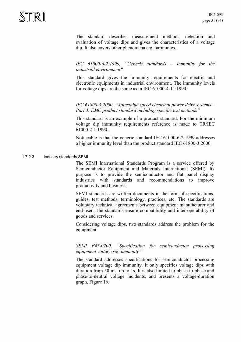
R02-093 page 31 (94)

The standard describes measurement methods, detection and evaluation of voltage dips and gives the characteristics of a voltage dip. It also covers other phenomena e.g. harmonics.

IEC 61000-6-2:1999, “Generic standards – Immunity for the industrial environment” This standard gives the immunity requirements for electric and electronic equipments in industrial environment. The immunity levels for voltage dips are the same as in IEC 61000-4-11:1994.

IEC 61800-3:2000, “Adjustable speed electrical power drive systems – Part 3: EMC product standard including specific test methods” This standard is an example of a product standard. For the minimum voltage dip immunity requirements reference is made to TR/IEC 61000-2-1:1990.

Noticeable is that the generic standard IEC 61000-6-2:1999 addresses a higher immunity level than the product standard IEC 61800-3:2000.

1.7.2.3 Industry standards SEMI The SEMI International Standards Program is a service offered by Semiconductor Equipment and Materials International (SEMI). Its purpose is to provide the semiconductor and flat panel display industries with standards and recommendations to improve productivity and business.

SEMI standards are written documents in the form of specifications, guides, test methods, terminology, practices, etc. The standards are voluntary technical agreements between equipment manufacturer and end-user. The standards ensure compatibility and inter-operability of goods and services.

Considering voltage dips, two standards address the problem for the equipment.

SEMI F47-0200, “Specification for semiconductor processing equipment voltage sag immunity” The standard addresses specifications for semiconductor processing equipment voltage dip immunity. It only specifies voltage dips with duration from 50 ms. up to 1s. It is also limited to phase-to-phase and phase-to-neutral voltage incidents, and presents a voltage-duration graph, Figure 16.

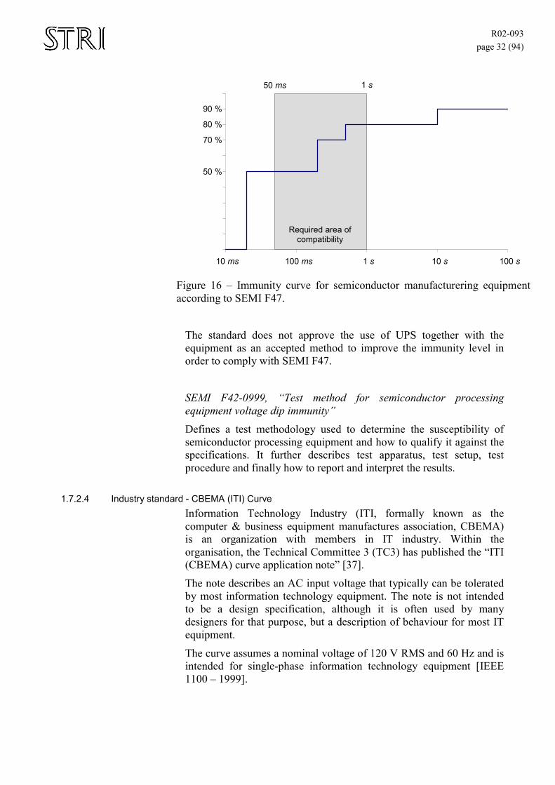
R02-093 page 32 (94)

Figure 16 – Immunity curve for semiconductor manufacturering equipment according to SEMI F47.

The standard does not approve the use of UPS together with the equipment as an accepted method to improve the immunity level in order to comply with SEMI F47.

SEMI F42-0999, “Test method for semiconductor processing equipment voltage dip immunity”

Defines a test methodology used to determine the susceptibility of semiconductor processing equipment and how to qualify it against the specifications. It further describes test apparatus, test setup, test procedure and finally how to report and interpret the results.

1.7.2.4 Industry standard - CBEMA (ITI) Curve Information Technology Industry (ITI, formally known as the computer & business equipment manufactures association, CBEMA) is an organization with members in IT industry. Within the organisation, the Technical Committee 3 (TC3) has published the “ITI (CBEMA) curve application note” [37]. The note describes an AC input voltage that typically can be tolerated by most information technology equipment. The note is not intended to be a design specification, although it is often used by many designers for that purpose, but a description of behaviour for most IT equipment.

The curve assumes a nominal voltage of 120 V RMS and 60 Hz and is intended for single-phase information technology equipment [IEEE 1100 – 1999].

50 %

70 % 80 % 90 %

10 ms 100 ms 1 s 10 s 100 s

Required area of compatibility

50 ms 1 s

R02-093 page 33 (94)

The voltage-time curve describes the border of an area. Above the border the equipment shall work properly and below shall it shutdown in a controlled way, Figure 17.

Figure 17 – Revised CBEMA curve, ITIC curve, 1996 [37].

1.7.3 Differences between the standards The IEEE standards are written to give guidance and focus more on the system than single components. The IEC 61000 standards are written to give a thorough background, and from that develop new component and equipment dedicated standards.

1.8. Conclusion

1.8.1 Description of voltage dips The descriptions of voltage dips have to be improved compared to the methods used today. Using only RMS-values and durations, is not enough to describe all properties of the voltage dip. It is not possible, based on such limited information, to conclude how three-phase systems and equipment will behave and decide whether a voltage dip is harmful or not.

A new, and more accurate approach to voltage dips is to consider them as a three-phase rather than a single-phase phenomenon. Such approach will give information about the magnitude and angle of all phases, giving a more realistic picture of the voltage dip.

70% 80% 90%

1 ms 10 ms 0,1 s 1 s 10 s 100 s

R02-093 page 34 (94)

For some applications and studies, the single-phase representation is accurate enough and there is no need for a more advanced description. A major advantage with the three-phase description is that different types of voltage dips can be studied (actually 7 different types described in “Voltage dip classification”) and knowledge of point-on-wave where the voltage dip occurred can be obtained. Many kinds of loads, with low immunity and high cost associated to a stop caused by a voltage dip, are three-phases connected.

One advantage with the voltage-duration chart is also that it is rather easy to compare voltage dip immunity of different equipment with each other using voltage-duration plots, ITI, SEMI etc. A new and more complex method has to be developed for the three-phase description of equipment voltage dip immunity. But it still has to be easy to use.

1.8.2 Equipment sensitivity Generally many kinds of new equipment have become more sensitive to voltage dips than before. One of the main reasons to the increased susceptibility is the use of power electronics in many applications. Despite that the immunity has decreased, a proper design, with a correct use of the power electronics, can improve the ride-through capacity of the equipment. New techniques, in control design, larger energy storage (but not batteries), faster measurements and data processing, offer lots of potential to improve the immunity.

The manufacturer shall be able to provide information about the voltage dip ride-through capatibility of his products to the customer.

1.8.3 Standards There are many standards dealing with power quality. Some of them are written to give guidance about how to achieve higher immunity against disturbances, and often describe entire systems. Others are developed with the purpose to be used as requirements, and focus on single components and the surrounding environment. A common problem is that voltage dips are considered as a single-phase, instead of a multiple-phase phenomenon.

In the future, standards need to be more product specific. They also need to better classify the voltage dip immunity level for the product. Today there are only a few equipment immunity requirements against voltage dips.

R02-093 page 35 (94)

R02-093 page 36 (94)

2 Characterisation of voltage dip activity at the site Working with voltage dip disturbances at a site requires knowledge of the frequency and characteristics of the voltage dips occurring at the location. The first step for characterisation is therefore to collect and analyse data to obtain information of the voltage dip characteristics at the site. The result will lead to a better understanding and possibilities to compare different mitigation solutions. It is also necessary to do this inventory to estimate the cost from voltage dips and the number of disturbances, making different mitigation actions valuable according to the cost. A proper characterisation can also be used to test the sub-processes with voltage dips similar to the ones that occur at the site.

2.1. Voltage dip sources Voltage dips are the result of condition changes in the utility grid or the local network [32]. Voltage dips due to changes in the feeding grid are denoted ‘remotely injected voltage dips’, and voltage dips due to changes in the local network are denoted ‘locally injected voltage dips’.

2.1.1 Remotely injected voltage dips Short circuits are the main cause for voltage dips originating from the feeding grid. A voltage dip in the transmission grid will affect more customers than a fault in the distribution grid. Also a fault at the higher voltage levels is often cleared faster than at the distribution level. The problem with voltage dips originating at higher voltage levels, is that the voltage dips will propagate far away from the origin, affecting a large number of customers.

Remotely injected voltage dips are often severe and can cause disturbances to connected systems.

2.1.2 Locally injected voltage dips Locally injected voltage dips can be caused by faults or load changes inside the plant network. Load changes will often result in less severe voltage dips than those caused by a fault. In some cases, local injected voltage dips only affect a few busbars.

2.2. Measurement The best way to determine the voltage dip characteristics at the site is to perform measurements. Measurements can be performed having two objectives in mind. The first is to see how the feeding grid responds to different faults, and the second is to see how specific equipment behaves during a voltage dip. For this reason the measuring equipment shall be equipped with extra analogue and digital inputs to be used for measuring speed, torque, temperature etc. To be able to observe the propagation of a voltage dip, it is necessary to have more than one monitor located at

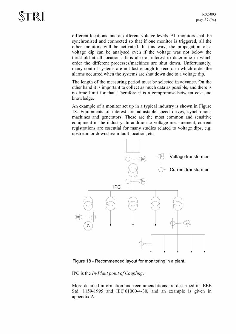
R02-093 page 37 (94)

different locations, and at different voltage levels. All monitors shall be synchronised and connected so that if one monitor is triggered, all the other monitors will be activated. In this way, the propagation of a voltage dip can be analysed even if the voltage was not below the threshold at all locations. It is also of interest to determine in which order the different processes/machines are shut down. Unfortunately, many control systems are not fast enough to record in which order the alarms occurred when the systems are shut down due to a voltage dip.

The length of the measuring period must be selected in advance. On the other hand it is important to collect as much data as possible, and there is no time limit for that. Therefore it is a compromise between cost and knowledge.

An example of a monitor set up in a typical industry is shown in Figure 18. Equipments of interest are adjustable speed drives, synchronous machines and generators. These are the most common and sensitive equipment in the industry. In addition to voltage measurement, current registrations are essential for many studies related to voltage dips, e.g. upstream or downstream fault location, etc.

G

Voltage transformer

Current transformer

IPC

Figure 18 - Recommended layout for monitoring in a plant.

IPC is the In-Plant point of Coupling.

More detailed information and recommendations are described in IEEE Std. 1159-1995 and IEC 61000-4-30, and an example is given in appendix A.

R02-093 page 38 (94)

2.3. Determining voltage dip activity Voltage dip activity information at the specific location is necessary in order to perform any analysis of related problems for the site and finding cost effective solutions. There are different ways to obtain the information. Either the information is provided by the utility, or a study is conducted by either the customer or the utility. Regardless of who performs the study, the principles are almost the same.

There are three different ways to obtain data. The first one is by measurements and then handle the data statistically. The second is a stochastic approach to estimate the voltage dip activity. A third way is to obtain guidelines based on typical values from other studies.

It is also necessary to separate locally injected voltage dips from remotely injected.

2.3.1 Data from measurements Data from actual measurements can be very accurate if they are conducted over a long time. The data are however only correct as long as the feeding network remains unchanged or all changes are known. The statistics from measurements can also differ from year to year. There is also the possibility that there will be abnormalities and other factors that will have radical impact on the data. E.g. a year with a lot of storms and hot weather is likely to have more disturbances than a calmer and cooler year. Measurements can therefore never provide a complete understanding of the voltage dip activity at a site. It can however describe the different characteristics and types of voltage dips.

Another parameter of importance is at which point the data are measured. An optimal case is when data are provided by the utility and measured at IPC (In-plant Point of Coupling). Another alternative it is to perform measurements at substations, on busbars inside the plant, on machines, other similar sites, etc. Ideally, voltages and currents are measured at different voltage levels and locations inside and outside the plant.

It is also very important to remember that the measured data can be used for voltage dip propagation studies on the network inside the plant. The same voltage dip may have different characteristics in different locations in the plant, due to different connections and loads.

It can be very uncertain to rely only on historical data. New configurations, climate changes, new equipment, can lead to changed characteristic and activity.

2.3.2 Data from stochastic predictions of voltage dips An alternative way to describe the voltage dip environment and activity is to perform a stochastic analysis. The evaluation is based on knowledge of the system configuration and failure rates of different equipment. Other factors like fault clearing time, service, maintenance,

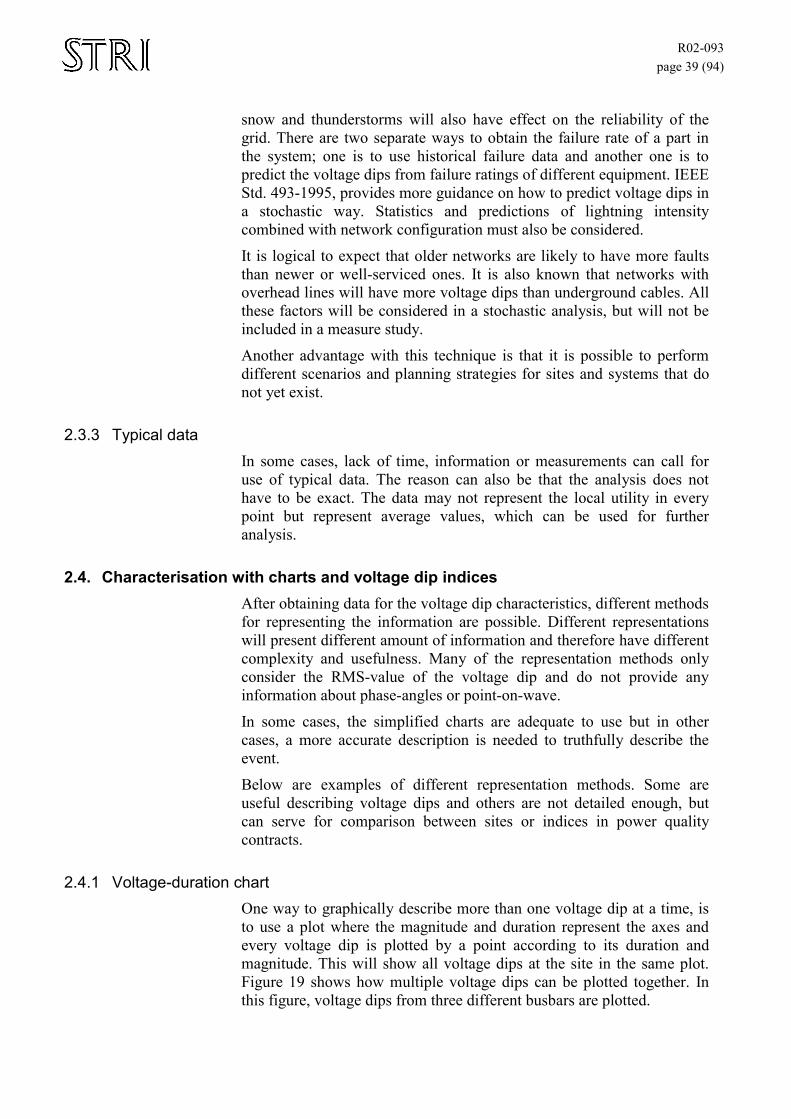
R02-093 page 39 (94)

snow and thunderstorms will also have effect on the reliability of the grid. There are two separate ways to obtain the failure rate of a part in the system; one is to use historical failure data and another one is to predict the voltage dips from failure ratings of different equipment. IEEE Std. 493-1995, provides more guidance on how to predict voltage dips in a stochastic way. Statistics and predictions of lightning intensity combined with network configuration must also be considered.

It is logical to expect that older networks are likely to have more faults than newer or well-serviced ones. It is also known that networks with overhead lines will have more voltage dips than underground cables. All these factors will be considered in a stochastic analysis, but will not be included in a measure study.

Another advantage with this technique is that it is possible to perform different scenarios and planning strategies for sites and systems that do not yet exist.

2.3.3 Typical data In some cases, lack of time, information or measurements can call for use of typical data. The reason can also be that the analysis does not have to be exact. The data may not represent the local utility in every point but represent average values, which can be used for further analysis.

2.4. Characterisation with charts and voltage dip indices After obtaining data for the voltage dip characteristics, different methods for representing the information are possible. Different representations will present different amount of information and therefore have different complexity and usefulness. Many of the representation methods only consider the RMS-value of the voltage dip and do not provide any information about phase-angles or point-on-wave.

In some cases, the simplified charts are adequate to use but in other cases, a more accurate description is needed to truthfully describe the event.

Below are examples of different representation methods. Some are useful describing voltage dips and others are not detailed enough, but can serve for comparison between sites or indices in power quality contracts.

2.4.1 Voltage-duration chart One way to graphically describe more than one voltage dip at a time, is to use a plot where the magnitude and duration represent the axes and every voltage dip is plotted by a point according to its duration and magnitude. This will show all voltage dips at the site in the same plot. Figure 19 shows how multiple voltage dips can be plotted together. In this figure, voltage dips from three different busbars are plotted.

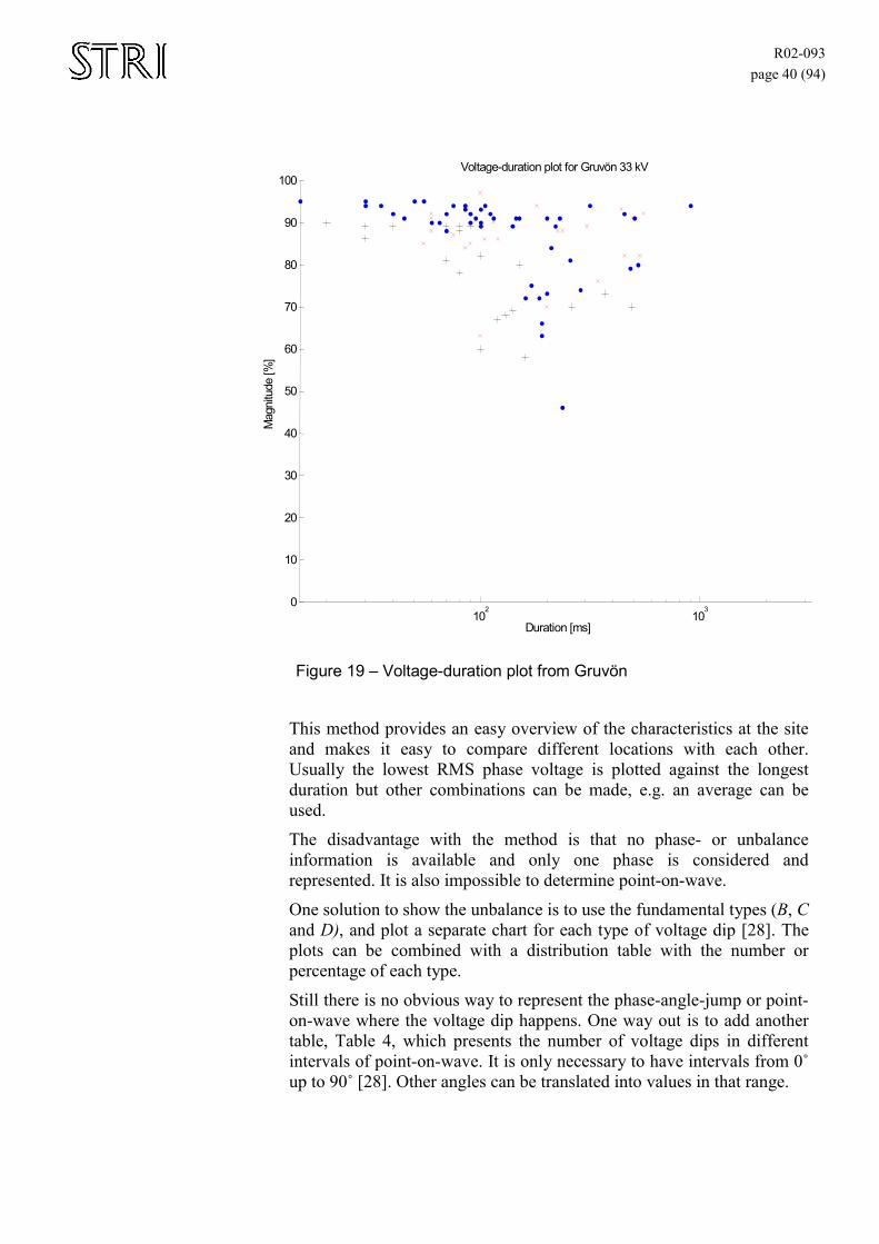
R02-093 page 40 (94)

10 2 10 3 0 10 20 30 40 50 60 70 80 90

100 Voltage-duration plot for Gruvön 33 kV

Duration [ms]

Mag

nitu

de [%

]

Figure 19 – Voltage-duration plot from Gruvön

This method provides an easy overview of the characteristics at the site and makes it easy to compare different locations with each other. Usually the lowest RMS phase voltage is plotted against the longest duration but other combinations can be made, e.g. an average can be used.

The disadvantage with the method is that no phase- or unbalance information is available and only one phase is considered and represented. It is also impossible to determine point-on-wave.

One solution to show the unbalance is to use the fundamental types (B, C and D), and plot a separate chart for each type of voltage dip [28]. The plots can be combined with a distribution table with the number or percentage of each type.

Still there is no obvious way to represent the phase-angle-jump or point-on-wave where the voltage dip happens. One way out is to add another table, Table 4, which presents the number of voltage dips in different intervals of point-on-wave. It is only necessary to have intervals from 0˚ up to 90˚ [28]. Other angles can be translated into values in that range.

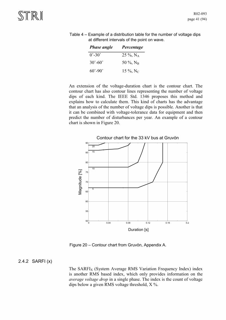
R02-093 page 41 (94)

Table 4 – Example of a distribution table for the number of voltage dips at different intervals of the point on wave.

Phase angle Percentage

0˚-30˚ 25 %, NA

30˚-60˚ 50 %, NB

60˚-90˚ 15 %, NC

An extension of the voltage-duration chart is the contour chart. The contour chart has also contour lines representing the number of voltage dips of each kind. The IEEE Std. 1346 proposes this method and explains how to calculate them. This kind of charts has the advantage that an analysis of the number of voltage dips is possible. Another is that it can be combined with voltage-tolerance data for equipment and then predict the number of disturbances per year. An example of a contour chart is shown in Figure 20.

Figure 20 – Contour chart from Gruvön, Appendix A.

2.4.2 SARFI (x) The SARFIX (System Average RMS Variation Frequency Index) index is another RMS based index, which only provides information on the average voltage drop in a single phase. The index is the count of voltage dips below a given RMS voltage threshold, X %.

0 0.04 0.08 0.12 0.16 0.2 50

55

60

65

70

75

80

85

90

5

10

15 20

Mag

nitu

de [%

]

Duration [s]

Contour chart for the 33 kV bus at Gruvön

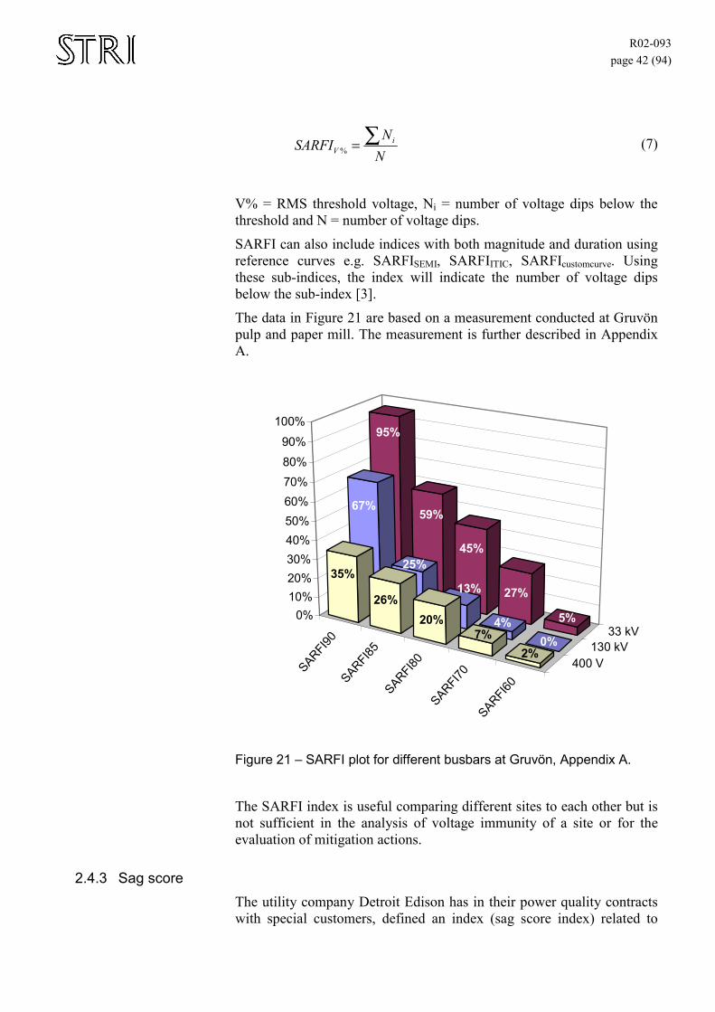
R02-093 page 42 (94)

NN

SARFI iV

∑=% (7)

V% = RMS threshold voltage, Ni = number of voltage dips below the threshold and N = number of voltage dips.

SARFI can also include indices with both magnitude and duration using reference curves e.g. SARFISEMI, SARFIITIC, SARFIcustomcurve. Using these sub-indices, the index will indicate the number of voltage dips below the sub-index [3].

The data in Figure 21 are based on a measurement conducted at Gruvön pulp and paper mill. The measurement is further described in Appendix A.

SARFI90

SARFI85

SARFI80

SARFI70

SARFI60

400 V130 kV

33 kV

95%

59%

45%

27%

5%

67%

25%

13%

4%0%

35%

26%20%

7%2%

0%10%20%30%40%50%60%70%80%90%

100%

Figure 21 – SARFI plot for different busbars at Gruvön, Appendix A.

The SARFI index is useful comparing different sites to each other but is not sufficient in the analysis of voltage immunity of a site or for the evaluation of mitigation actions.

2.4.3 Sag score The utility company Detroit Edison has in their power quality contracts with special customers, defined an index (sag score index) related to

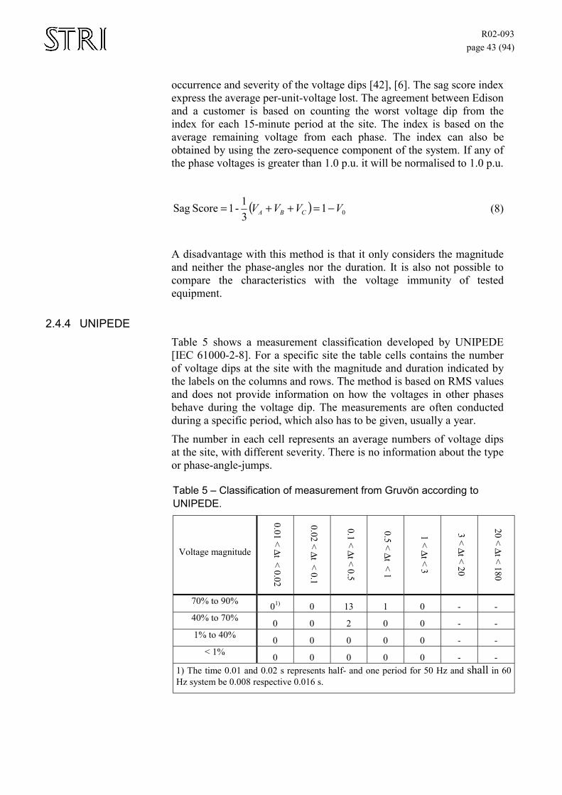
R02-093 page 43 (94)

occurrence and severity of the voltage dips [42], [6]. The sag score index express the average per-unit-voltage lost. The agreement between Edison and a customer is based on counting the worst voltage dip from the index for each 15-minute period at the site. The index is based on the average remaining voltage from each phase. The index can also be obtained by using the zero-sequence component of the system. If any of the phase voltages is greater than 1.0 p.u. it will be normalised to 1.0 p.u.

( ) 0131-1Score Sag VVVV CBA −=++= (8)

A disadvantage with this method is that it only considers the magnitude and neither the phase-angles nor the duration. It is also not possible to compare the characteristics with the voltage immunity of tested equipment.

2.4.4 UNIPEDE Table 5 shows a measurement classification developed by UNIPEDE [IEC 61000-2-8]. For a specific site the table cells contains the number of voltage dips at the site with the magnitude and duration indicated by the labels on the columns and rows. The method is based on RMS values and does not provide information on how the voltages in other phases behave during the voltage dip. The measurements are often conducted during a specific period, which also has to be given, usually a year.

The number in each cell represents an average numbers of voltage dips at the site, with different severity. There is no information about the type or phase-angle-jumps.

Table 5 – Classification of measurement from Gruvön according to UNIPEDE.

Voltage magnitude

0.01 < ∆t < 0.02

0.02 < ∆t < 0.1

0.1 < ∆t < 0.5

0.5 < ∆t < 1

1 < ∆t < 3

3 < ∆t < 20

20 < ∆t < 180

70% to 90% 01) 0 13 1 0 - - 40% to 70% 0 0 2 0 0 - - 1% to 40% 0 0 0 0 0 - -

< 1% 0 0 0 0 0 - - 1) The time 0.01 and 0.02 s represents half- and one period for 50 Hz and shall in 60 Hz system be 0.008 respective 0.016 s.

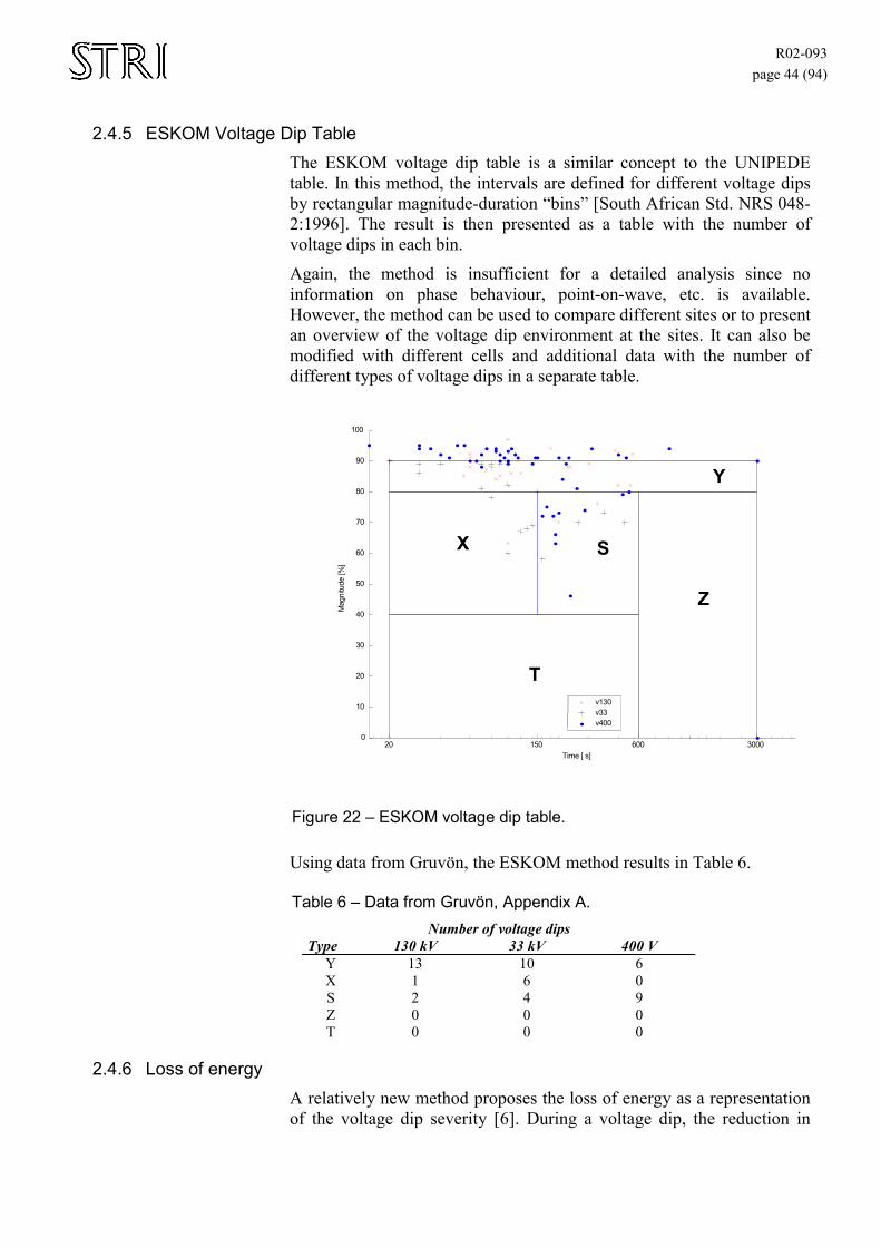
R02-093 page 44 (94)

2.4.5 ESKOM Voltage Dip Table The ESKOM voltage dip table is a similar concept to the UNIPEDE table. In this method, the intervals are defined for different voltage dips by rectangular magnitude-duration “bins” [South African Std. NRS 048-2:1996]. The result is then presented as a table with the number of voltage dips in each bin.

Again, the method is insufficient for a detailed analysis since no information on phase behaviour, point-on-wave, etc. is available. However, the method can be used to compare different sites or to present an overview of the voltage dip environment at the sites. It can also be modified with different cells and additional data with the number of different types of voltage dips in a separate table.

20 150 600 3000 0 10 20 30 40 50 60 70 80 90

100

Time [ s]

Mag

nitu

de [%

]

v130 v33 v400

T

X S

Z

Y

Figure 22 – ESKOM voltage dip table.

Using data from Gruvön, the ESKOM method results in Table 6.

Table 6 – Data from Gruvön, Appendix A. Number of voltage dips

Type 130 kV 33 kV 400 V Y 13 10 6 X 1 6 0 S 2 4 9 Z 0 0 0 T 0 0 0

2.4.6 Loss of energy A relatively new method proposes the loss of energy as a representation of the voltage dip severity [6]. During a voltage dip, the reduction in

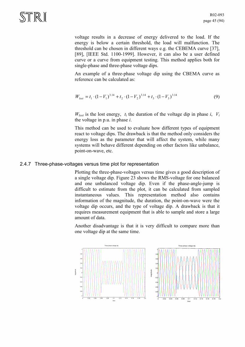
R02-093 page 45 (94)

voltage results in a decrease of energy delivered to the load. If the energy is below a certain threshold, the load will malfunction. The threshold can be chosen in different ways e.g. the CEBEMA curve [37], [89], [IEEE Std. 1100-1999]. However, it can also be a user defined curve or a curve from equipment testing. This method applies both for single-phase and three-phase voltage dips.

An example of a three-phase voltage dip using the CBEMA curve as reference can be calculated as:

14.3

3314.3

2214.3

11 )1()1()1( VtVtVtWlost −⋅+−⋅+−⋅= (9)

Wlost is the lost energy, ti the duration of the voltage dip in phase i, Vi the voltage in p.u. in phase i. This method can be used to evaluate how different types of equipment react to voltage dips. The drawback is that the method only considers the energy loss as the parameter that will affect the system, while many systems will behave different depending on other factors like unbalance, point-on-wave, etc.

2.4.7 Three-phase-voltages versus time plot for representation Plotting the three-phase-voltages versus time gives a good description of a single voltage dip. Figure 23 shows the RMS-voltage for one balanced and one unbalanced voltage dip. Even if the phase-angle-jump is difficult to estimate from the plot, it can be calculated from sampled instantaneous values. This representation method also contains information of the magnitude, the duration, the point-on-wave were the voltage dip occurs, and the type of voltage dip. A drawback is that it requires measurement equipment that is able to sample and store a large amount of data.

Another disadvantage is that it is very difficult to compare more than one voltage dip at the same time.

0 0.02 0.04 0.06 0.08 0.1 0.12 0.14 0.16 0.18 0.2 -1 -0.8 -0.6 -0.4 -0.2

0 0.2 0.4 0.6 0.8

1 Three phase voltage dip

mag

nitu

de

time 0 0.02 0.04 0.06 0.08 0.1 0.12 0.14 0.16 0.18 0.2 -1 -0.8 -0.6 -0.4 -0.2 0

0.2 0.4 0.6 0.8 1 Three phase voltage dip

mag

nitu

de

time

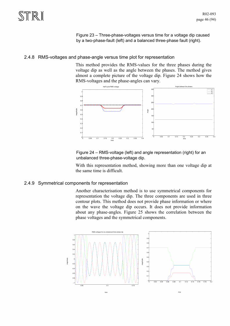
R02-093 page 46 (94)

Figure 23 – Three-phase-voltages versus time for a voltage dip caused by a two-phase-fault (left) and a balanced three-phase fault (right).

2.4.8 RMS-voltages and phase-angle versus time plot for representation This method provides the RMS-values for the three phases during the voltage dip as well as the angle between the phases. The method gives almost a complete picture of the voltage dip. Figure 24 shows how the RMS-voltages and the phase-angles can vary.

0 0.05 0.1 0.15 0.2 0.25 0.3 0.35 0.4 0 0.1 0.2 0.3 0.4 0.5 0.6 0.7 0.8 0.9

1 Half-cycle RMS voltage

mag

nitu

de

time

0 0.05 0.1 0.15 0.2 0.25 0.3 0.35 0.4 0 50

100 150 200 250 300 350 Angle between the phases

u1 u2 u3

Angl

e

time

Figure 24 – RMS-voltage (left) and angle representation (right) for an unbalanced three-phase-voltage dip.

With this representation method, showing more than one voltage dip at the same time is difficult.

2.4.9 Symmetrical components for representation Another characterisation method is to use symmetrical components for representation the voltage dip. The three components are used in three contour plots. This method does not provide phase information or where on the wave the voltage dip occurs. It does not provide information about any phase-angles. Figure 25 shows the correlation between the phase voltages and the symmetrical components.

0.05 0.1 0.15 -1 -0.8 -0.6 -0.4 -0.2

0 0.2 0.4 0.6 0.8

1

time

mag

nitu

de

RMS-voltages for an unbalanced three phase dip

0 0.02 0.04 0.06 0.08 0.1 0.12 0.14 0.16 0.18 0.2 0 0.1 0.2 0.3 0.4 0.5 0.6 0.7 0.8 0.9

1

time

mag

nitu

de

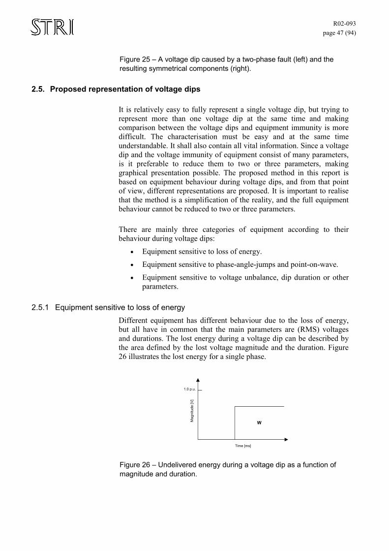
R02-093 page 47 (94)

Figure 25 – A voltage dip caused by a two-phase fault (left) and the resulting symmetrical components (right).

2.5. Proposed representation of voltage dips

It is relatively easy to fully represent a single voltage dip, but trying to represent more than one voltage dip at the same time and making comparison between the voltage dips and equipment immunity is more difficult. The characterisation must be easy and at the same time understandable. It shall also contain all vital information. Since a voltage dip and the voltage immunity of equipment consist of many parameters, is it preferable to reduce them to two or three parameters, making graphical presentation possible. The proposed method in this report is based on equipment behaviour during voltage dips, and from that point of view, different representations are proposed. It is important to realise that the method is a simplification of the reality, and the full equipment behaviour cannot be reduced to two or three parameters.

There are mainly three categories of equipment according to their behaviour during voltage dips:

• Equipment sensitive to loss of energy.

• Equipment sensitive to phase-angle-jumps and point-on-wave.

• Equipment sensitive to voltage unbalance, dip duration or other parameters.

2.5.1 Equipment sensitive to loss of energy Different equipment has different behaviour due to the loss of energy, but all have in common that the main parameters are (RMS) voltages and durations. The lost energy during a voltage dip can be described by the area defined by the lost voltage magnitude and the duration. Figure 26 illustrates the lost energy for a single phase.

Time [ms]

Mag

nitu

de [V

]

W

1.0 p.u.

Figure 26 – Undelivered energy during a voltage dip as a function of magnitude and duration.

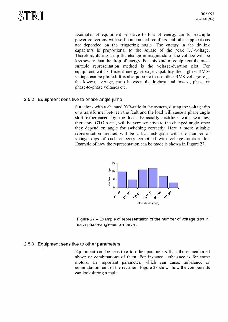
R02-093 page 48 (94)

Examples of equipment sensitive to loss of energy are for example power converters with self-comutatated rectifiers and other applications not depended on the triggering angle. The energy in the dc-link capacitors is proportional to the square of the peak DC-voltage. Therefore, during a dip the change in magnitude of the voltage will be less severe than the drop of energy. For this kind of equipment the most suitable representation method is the voltage-duration plot. For equipment with sufficient energy storage capability the highest RMS-voltage can be plotted. It is also possible to use other RMS voltages e.g. the lowest, average, ratio between the highest and lowest, phase or phase-to-phase voltages etc.

2.5.2 Equipment sensitive to phase-angle-jump Situations with a changed X/R-ratio in the system, during the voltage dip or a transformer between the fault and the load will cause a phase-angle shift experienced by the load. Especially rectifiers with switches, thyristors, GTO´s etc., will be very sensitive to the changed angle since they depend on angle for switching correctly. Here a more suitable representation method will be a bar histogram with the number of voltage dips of each category combined with voltage-duration-plot. Example of how the representation can be made is shown in Figure 27.

0

5

10

15

Intervals [degrees]

Num

ber o

f dip

s

Figure 27 – Example of representation of the number of voltage dips in each phase-angle-jump interval.

2.5.3 Equipment sensitive to other parameters Equipment can be sensitive to other parameters than those mentioned above or combinations of them. For instance, unbalance is for some motors, an important parameter, which can cause unbalance or commutation fault of the rectifier. Figure 28 shows how the components can look during a fault.

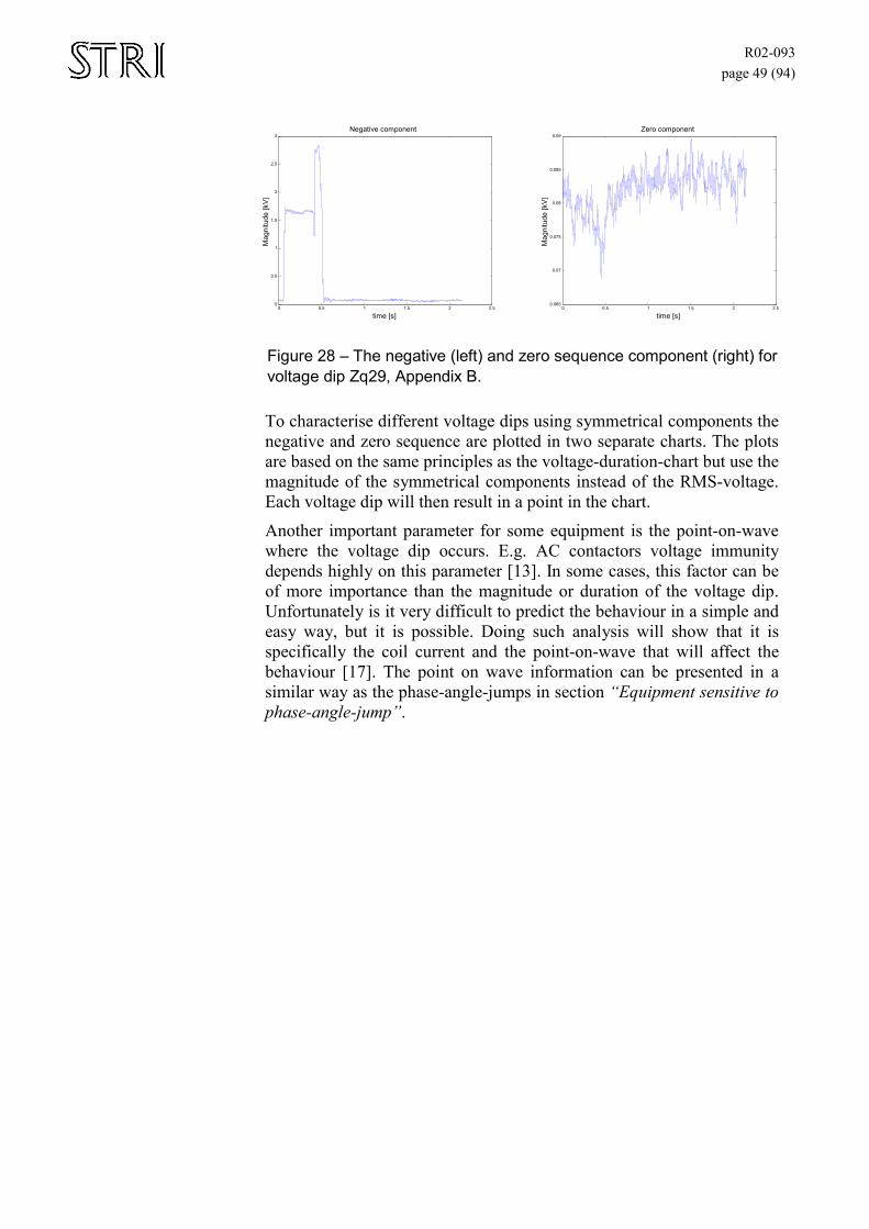
R02-093 page 49 (94)

0 0.5 1 1.5 2 2.5 0 0.5

1 1.5

2 2.5

3 Negative component

time [s]

Mag

nitu

de [k

V]

0 0.5 1 1.5 2 2.5 0.065

0.07

0.075

0.08

0.085

0.09 Zero component

time [s]

Mag

nitu

de [k

V]

Figure 28 – The negative (left) and zero sequence component (right) for voltage dip Zq29, Appendix B.

To characterise different voltage dips using symmetrical components the negative and zero sequence are plotted in two separate charts. The plots are based on the same principles as the voltage-duration-chart but use the magnitude of the symmetrical components instead of the RMS-voltage. Each voltage dip will then result in a point in the chart.

Another important parameter for some equipment is the point-on-wave where the voltage dip occurs. E.g. AC contactors voltage immunity depends highly on this parameter [13]. In some cases, this factor can be of more importance than the magnitude or duration of the voltage dip. Unfortunately is it very difficult to predict the behaviour in a simple and easy way, but it is possible. Doing such analysis will show that it is specifically the coil current and the point-on-wave that will affect the behaviour [17]. The point on wave information can be presented in a similar way as the phase-angle-jumps in section “Equipment sensitive to phase-angle-jump”.

R02-093 page 50 (94)

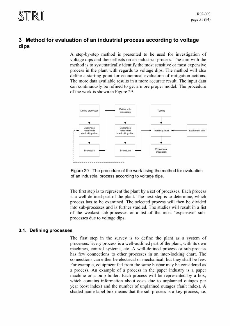
R02-093 page 51 (94)

3 Method for evaluation of an industrial process according to voltage dips

A step-by-step method is presented to be used for investigation of voltage dips and their effects on an industrial process. The aim with the method is to systematically identify the most sensitive or most expensive process in the plant with regards to voltage dips. The method will also define a starting point for economical evaluation of mitigation actions. The more data available results in a more accurate result. The input data can continuously be refined to get a more proper model. The procedure of the work is shown in Figure 29.

Define processes

Cost index Fault index

Interlocking chart

Evaluation

Define sub- processes

Cost index Fault index

Interlocking chart

Evaluation

Immunity level

Economical evaluation

Testing

Equipment data

Figure 29 - The procedure of the work using the method for evaluation of an industrial process according to voltage dips.

The first step is to represent the plant by a set of processes. Each process is a well-defined part of the plant. The next step is to determine, which process has to be examined. The selected process will then be divided into sub-processes and is further studied. The studies will result in a list of the weakest sub-processes or a list of the most ‘expensive’ sub-processes due to voltage dips.

3.1. Defining processes The first step in the survey is to define the plant as a system of processes. Every process is a well-outlined part of the plant, with its own machines, control systems, etc. A well-defined process or sub-process has few connections to other processes in an inter-locking chart. The connections can either be electrical or mechanical, but they shall be few. For example, equipment fed from the same busbar may be considered as a process. An example of a process in the paper industry is a paper machine or a pulp boiler. Each process will be represented by a box, which contains information about costs due to unplanned outages per year (cost index) and the number of unplanned outages (fault index). A shaded name label box means that the sub-process is a key-process, i.e.

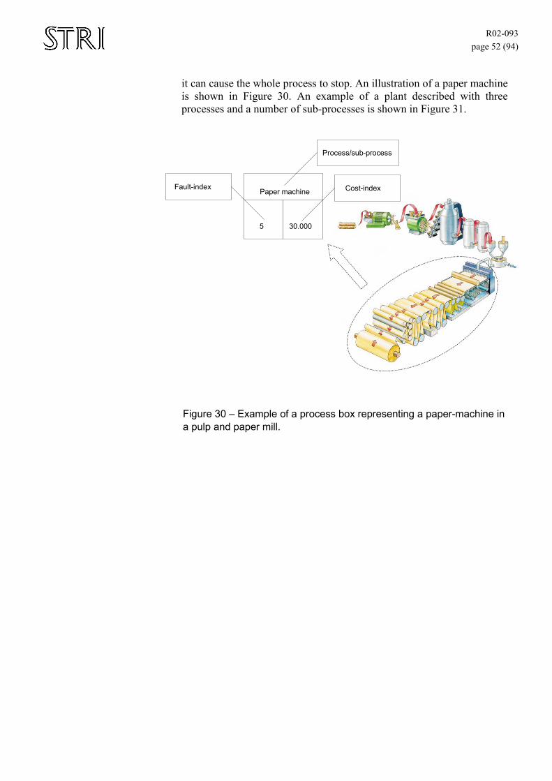
R02-093 page 52 (94)

it can cause the whole process to stop. An illustration of a paper machine is shown in Figure 30. An example of a plant described with three processes and a number of sub-processes is shown in Figure 31.

Process/sub-process

Cost-index Fault-index Paper machine

5 30.000

Figure 30 – Example of a process box representing a paper-machine in a pulp and paper mill.

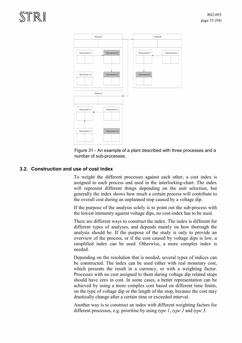
R02-093 page 53 (94)

Sub-process A.1

Sub-process A.3

Sub-process A.2

Sub-process A.4

Sub-process B.1

Sub-process B.3

Sub-process B.2

Sub-process C.1

Sub-process C.3

Sub-process C.2

Sub-process C.4

Process C

Process A Process B

Figure 31 - An example of a plant described with three processes and a number of sub-processes.

3.2. Construction and use of cost index To weight the different processes against each other, a cost index is assigned to each process and used in the interlocking-chart. The index will represent different things depending on the unit selection, but generally the index shows how much a certain process will contribute to the overall cost during an unplanned stop caused by a voltage dip.

If the purpose of the analysis solely is to point out the sub-process with the lowest immunity against voltage dips, no cost-index has to be used.

There are different ways to construct the index. The index is different for different types of analyses, and depends mainly on how thorough the analysis should be. If the purpose of the study is only to provide an overview of the process, or if the cost caused by voltage dips is low, a simplified index can be used. Otherwise, a more complex index is needed.

Depending on the resolution that is needed, several types of indices can be constructed. The index can be used either with real monetary cost, which presents the result in a currency, or with a weighting factor. Processes with no cost assigned to them during voltage dip related stops should have zero in cost. In some cases, a better representation can be achieved by using a more complex cost based on different time limits, on the type of voltage dip or the length of the stop, because the cost may drastically change after a certain time or exceeded interval.

Another way is to construct an index with different weighting factors for different processes, e.g. prioritise by using type 1, type 2 and type 3.

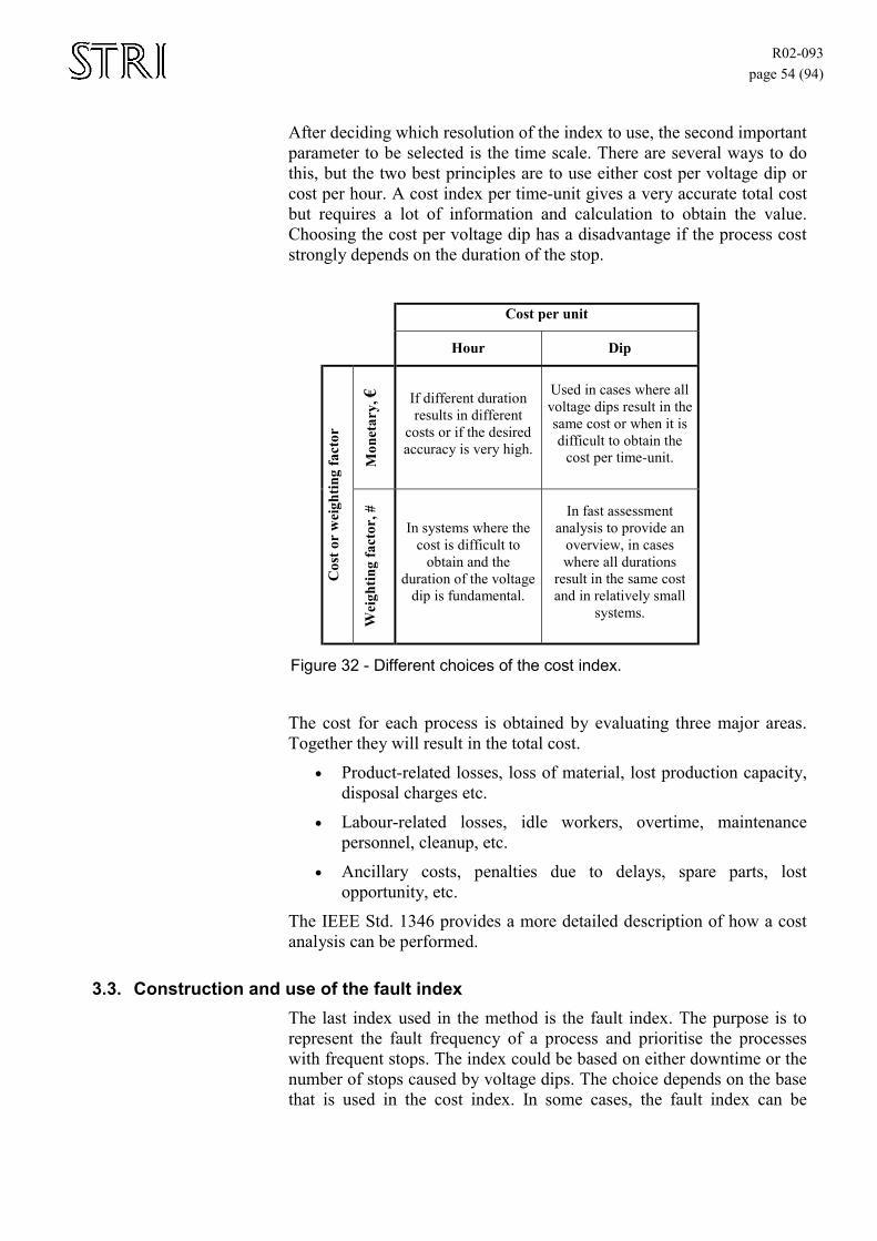
R02-093 page 54 (94)

After deciding which resolution of the index to use, the second important parameter to be selected is the time scale. There are several ways to do this, but the two best principles are to use either cost per voltage dip or cost per hour. A cost index per time-unit gives a very accurate total cost but requires a lot of information and calculation to obtain the value. Choosing the cost per voltage dip has a disadvantage if the process cost strongly depends on the duration of the stop.

Cost per unit

Hour Dip M

onet

ary,

€

If different duration results in different

costs or if the desired accuracy is very high.

Used in cases where all voltage dips result in the same cost or when it is difficult to obtain the

cost per time-unit.

Cos

t or

wei

ghtin

g fa

ctor

Wei

ghtin

g fa

ctor

, #

In systems where the cost is difficult to

obtain and the duration of the voltage

dip is fundamental.

In fast assessment analysis to provide an

overview, in cases where all durations

result in the same cost and in relatively small

systems.

Figure 32 - Different choices of the cost index.

The cost for each process is obtained by evaluating three major areas. Together they will result in the total cost.

• Product-related losses, loss of material, lost production capacity, disposal charges etc.

• Labour-related losses, idle workers, overtime, maintenance personnel, cleanup, etc.

• Ancillary costs, penalties due to delays, spare parts, lost opportunity, etc.

The IEEE Std. 1346 provides a more detailed description of how a cost analysis can be performed.

3.3. Construction and use of the fault index The last index used in the method is the fault index. The purpose is to represent the fault frequency of a process and prioritise the processes with frequent stops. The index could be based on either downtime or the number of stops caused by voltage dips. The choice depends on the base that is used in the cost index. In some cases, the fault index can be

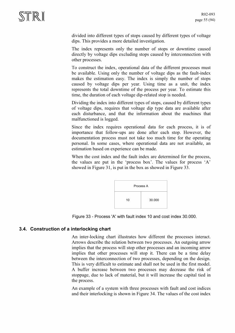
R02-093 page 55 (94)

divided into different types of stops caused by different types of voltage dips. This provides a more detailed investigation.

The index represents only the number of stops or downtime caused directly by voltage dips excluding stops caused by interconnection with other processes.

To construct the index, operational data of the different processes must be available. Using only the number of voltage dips as the fault-index makes the estimation easy. The index is simply the number of stops caused by voltage dips per year. Using time as a unit, the index represents the total downtime of the process per year. To estimate this time, the duration of each voltage dip-related stop is needed.

Dividing the index into different types of stops, caused by different types of voltage dips, requires that voltage dip type data are available after each disturbance, and that the information about the machines that malfunctioned is logged.

Since the index requires operational data for each process, it is of importance that follow-ups are done after each stop. However, the documentation process must not take too much time for the operating personal. In some cases, where operational data are not available, an estimation based on experience can be made.

When the cost index and the fault index are determined for the process, the values are put in the ‘process box’. The values for process ‘A’ showed in Figure 31, is put in the box as showed in Figure 33.

Process A

30.000 10

Figure 33 - Process 'A' with fault index 10 and cost index 30.000.

3.4. Construction of a interlocking chart An inter-locking chart illustrates how different the processes interact. Arrows describe the relation between two processes. An outgoing arrow implies that the process will stop other processes and an incoming arrow implies that other processes will stop it. There can be a time delay between the interconnection of two processes, depending on the design. This is very difficult to estimate and shall not be used in the first model. A buffer increase between two processes may decrease the risk of stoppage, due to lack of material, but it will increase the capital tied in the process.

An example of a system with three processes with fault and cost indices and their interlocking is shown in Figure 34. The values of the cost index

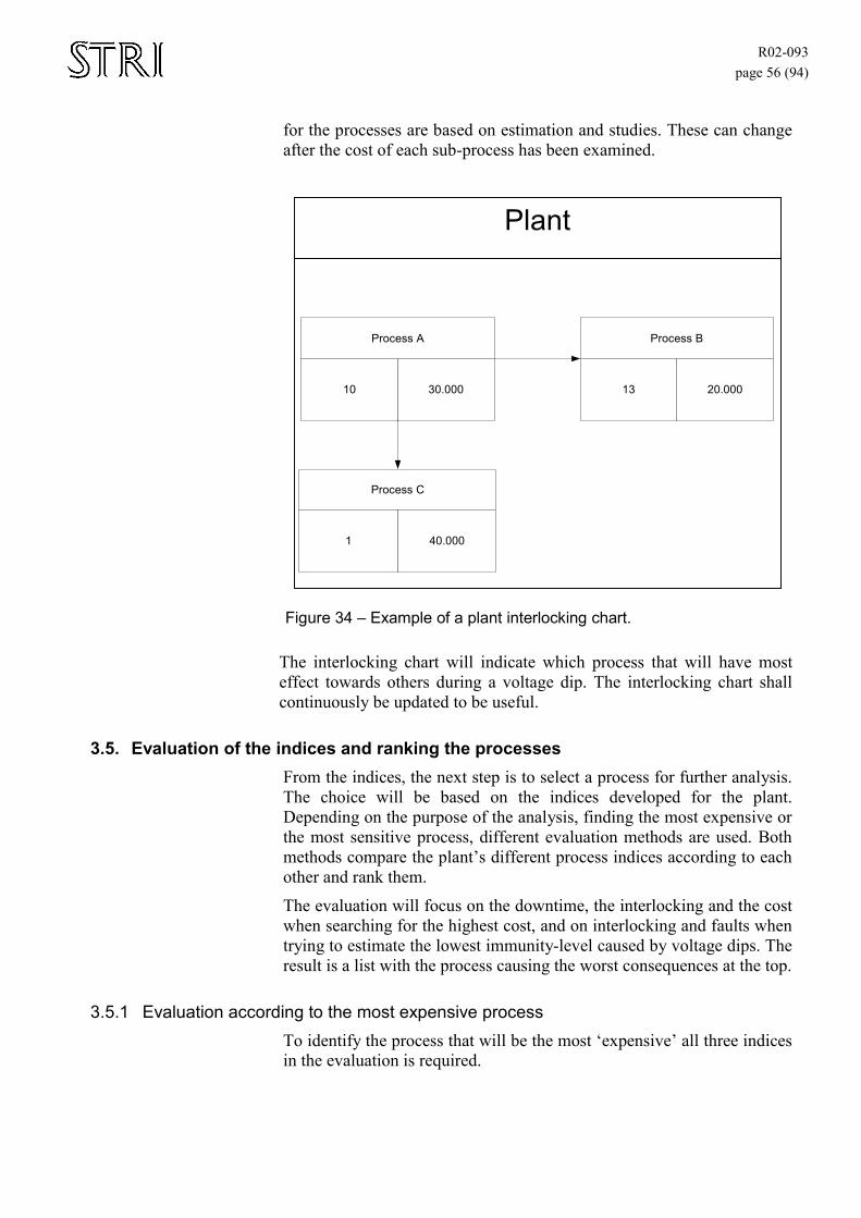
R02-093 page 56 (94)

for the processes are based on estimation and studies. These can change after the cost of each sub-process has been examined.

Process C

40.000 1

Process A

30.000 10

Process B

20.000 13

Plant

Figure 34 – Example of a plant interlocking chart.

The interlocking chart will indicate which process that will have most effect towards others during a voltage dip. The interlocking chart shall continuously be updated to be useful.

3.5. Evaluation of the indices and ranking the processes From the indices, the next step is to select a process for further analysis. The choice will be based on the indices developed for the plant. Depending on the purpose of the analysis, finding the most expensive or the most sensitive process, different evaluation methods are used. Both methods compare the plant’s different process indices according to each other and rank them.

The evaluation will focus on the downtime, the interlocking and the cost when searching for the highest cost, and on interlocking and faults when trying to estimate the lowest immunity-level caused by voltage dips. The result is a list with the process causing the worst consequences at the top.

3.5.1 Evaluation according to the most expensive process To identify the process that will be the most ‘expensive’ all three indices in the evaluation is required.

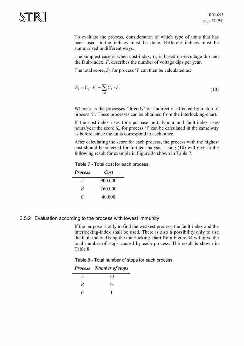
R02-093 page 57 (94)

To evaluate the process, consideration of which type of units that has been used in the indices must be done. Different indices must be summarised in different ways.

The simplest case is when cost-index, C, is based on €/voltage dip and the fault-index, F, describes the number of voltage dips per year.

The total score, Si, for process ‘i’ can then be calculated as:

∑ ⋅+⋅=}{k

ikiii FCFCS (10)

Where k is the processes ‘directly’ or ‘indirectly’ affected by a stop of process ‘i’. These processes can be obtained from the interlocking-chart.

If the cost-index uses time as base unit, €/hour and fault-index uses hours/year the score Si, for process ‘i’ can be calculated in the same way as before, since the units correspond to each other.

After calculating the score for each process, the process with the highest cost should be selected for further analysis. Using (10) will give in the following result for example in Figure 34 shown in Table 7.

Table 7 - Total cost for each process.

Process Cost

A 900.000

B 260.000

C 40.000

3.5.2 Evaluation according to the process with lowest immunity If the purpose is only to find the weakest process, the fault-index and the interlocking-index shall be used. There is also a possibility only to use the fault index. Using the interlocking-chart from Figure 34 will give the total number of stops caused by each process. The result is shown in Table 8.

Table 8 - Total number of stops for each process.

Process Number of stops

A 10

B 13

C 1

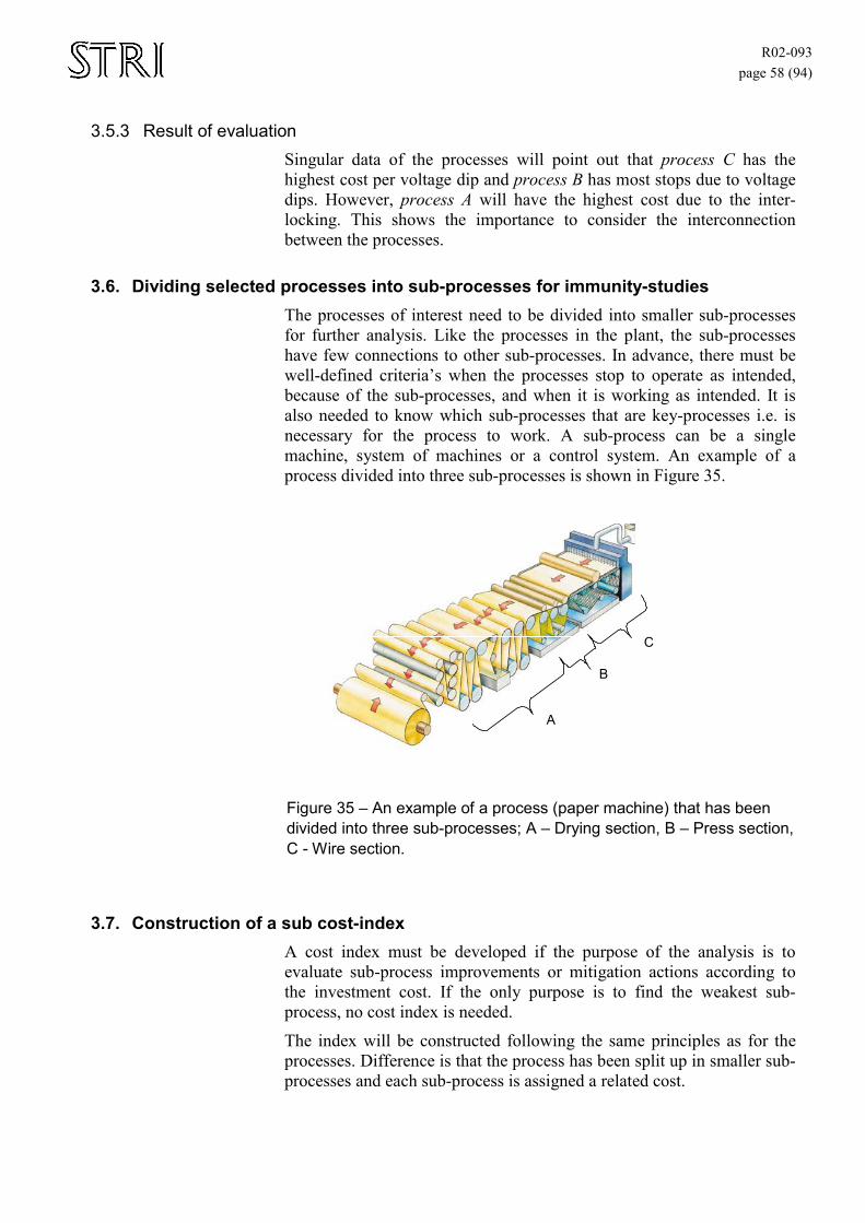
R02-093 page 58 (94)

3.5.3 Result of evaluation Singular data of the processes will point out that process C has the highest cost per voltage dip and process B has most stops due to voltage dips. However, process A will have the highest cost due to the inter-locking. This shows the importance to consider the interconnection between the processes.

3.6. Dividing selected processes into sub-processes for immunity-studies The processes of interest need to be divided into smaller sub-processes for further analysis. Like the processes in the plant, the sub-processes have few connections to other sub-processes. In advance, there must be well-defined criteria’s when the processes stop to operate as intended, because of the sub-processes, and when it is working as intended. It is also needed to know which sub-processes that are key-processes i.e. is necessary for the process to work. A sub-process can be a single machine, system of machines or a control system. An example of a process divided into three sub-processes is shown in Figure 35.

C

A

B

Figure 35 – An example of a process (paper machine) that has been divided into three sub-processes; A – Drying section, B – Press section, C - Wire section.

3.7. Construction of a sub cost-index A cost index must be developed if the purpose of the analysis is to evaluate sub-process improvements or mitigation actions according to the investment cost. If the only purpose is to find the weakest sub-process, no cost index is needed.

The index will be constructed following the same principles as for the processes. Difference is that the process has been split up in smaller sub-processes and each sub-process is assigned a related cost.

R02-093 page 59 (94)

3.8. Construction of a sub fault-index Again, a fault-index must be constructed, using the same principles as before. In this case, the index represents the number of stops of the different sub-processes. If no data are available, an estimation based on experience of the sub-process outages can be made.

3.9. Construction of a sub-process interlocking chart The chart will show how the sub-processes are connected to each other. As for the processes, each sub-process is represented by a box and with arrows between them.

Since the sub-cost and sub-fault indices are known, the real values of the fault and cost indices of the process can be calculated using (11) and (12). An example is shown in Figure 36. The values for process A may differ from estimated values in the earlier stages of the analysis.

4.2.1. AAAA FFFF ++= (11)

( )A

AAAAAAAAAAAA F

CFCFCCFCCCFC 4.43.3.4.2.2.4.2.1.1. )()( ⋅+⋅+++++= (12)

Sub-process A.1

1.500 3

Sub-process A.3

4.500 6

Sub-process A.2

25.000 2

Sub-process A.4

9.000 5

Process A

30.000 10

Figure 36 - A process consisting of four sub-processes.

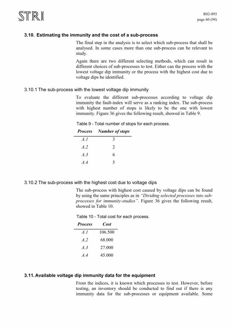
R02-093 page 60 (94)

3.10. Estimating the immunity and the cost of a sub-process The final step in the analysis is to select which sub-process that shall be analysed. In some cases more than one sub-process can be relevant to study.

Again there are two different selecting methods, which can result in different choices of sub-processes to test. Either can the process with the lowest voltage dip immunity or the process with the highest cost due to voltage dips be identified.

3.10.1 The sub-process with the lowest voltage dip immunity To evaluate the different sub-processes according to voltage dip immunity the fault-index will serve as a ranking index. The sub-process with highest number of stops is likely to be the one with lowest immunity. Figure 36 gives the following result, showed in Table 9.

Table 9 - Total number of stops for each process.

Process Number of stops

A.1 3

A.2 2

A.3 6

A.4 5

3.10.2 The sub-process with the highest cost due to voltage dips The sub-process with highest cost caused by voltage dips can be found by using the same principles as in “Dividing selected processes into sub-processes for immunity-studies”. Figure 36 gives the following result, showed in Table 10.

Table 10 - Total cost for each process.

Process Cost

A.1 106.500

A.2 68.000

A.3 27.000

A.4 45.000

3.11. Available voltage dip immunity data for the equipment From the indices, it is known which processes to test. However, before testing, an inventory should be conducted to find out if there is any immunity data for the sub-processes or equipment available. Some

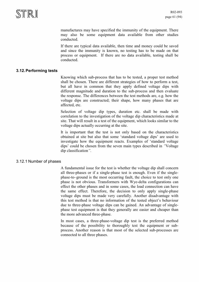
R02-093 page 61 (94)

manufactures may have specified the immunity of the equipment. There may also be some equipment data available from other studies conducted.

If there are typical data available, then time and money could be saved and since the immunity is known, no testing has to be made on that process or equipment. If there are no data available, testing shall be conducted.

3.12. Performing tests Knowing which sub-process that has to be tested, a proper test method shall be chosen. There are different strategies of how to perform a test, but all have in common that they apply defined voltage dips with different magnitude and duration to the sub-process and then evaluate the response. The differences between the test methods are, e.g. how the voltage dips are constructed; their shape, how many phases that are affected, etc.

Selection of voltage dip types, duration etc. shall be made with correlation to the investigation of the voltage dip characteristics made at site. That will result in a test of the equipment, which looks similar to the voltage dips actually occurring at the site.

It is important that the test is not only based on the characteristics obtained at site but also that some ‘standard voltage dips’ are used to investigate how the equipment reacts. Examples of ‘standard voltage dips’ could be chosen from the seven main types described in ”Voltage dip classification”.

3.12.1 Number of phases A fundamental issue for the test is whether the voltage dip shall concern all three-phases or if a single-phase test is enough. Even if the single-phase-to–ground is the most occurring fault, the choice to test only one phase is not obvious. Transformers with Wye-delta configurations can effect the other phases and in some cases, the load connection can have the same effect. Therefore, the decision to only apply single-phase voltage dips must be made very carefully. Another disadvantage with this test method is that no information of the tested object’s behaviour due to three-phase voltage dips can be gained. An advantage of single-phase test equipment is that they generally are easier and cheaper than the more advanced three-phase.

In most cases, a three-phase-voltage dip test is the preferred method because of the possibility to thoroughly test the equipment or sub-process. Another reason is that most of the selected sub-processes are connected to all three phases.

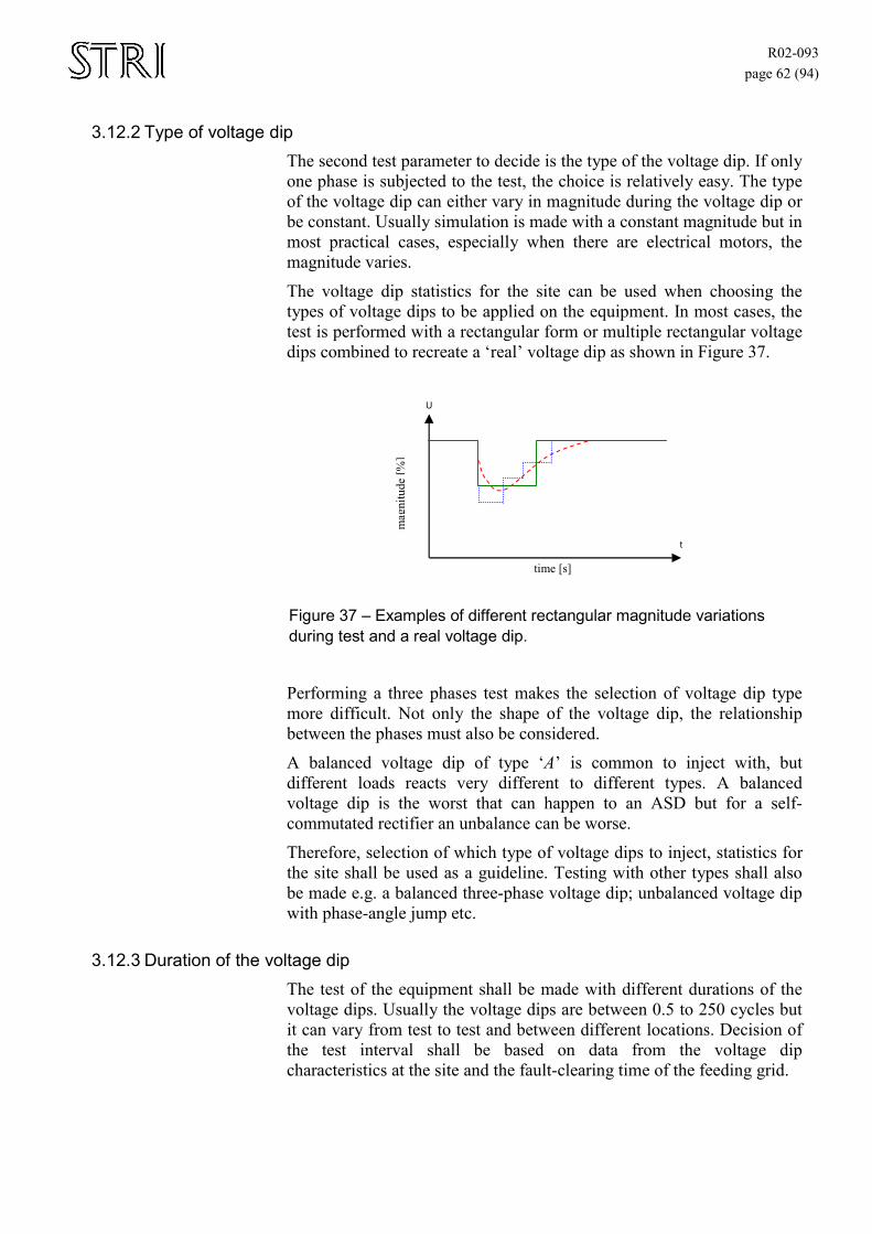
R02-093 page 62 (94)

3.12.2 Type of voltage dip The second test parameter to decide is the type of the voltage dip. If only one phase is subjected to the test, the choice is relatively easy. The type of the voltage dip can either vary in magnitude during the voltage dip or be constant. Usually simulation is made with a constant magnitude but in most practical cases, especially when there are electrical motors, the magnitude varies.

The voltage dip statistics for the site can be used when choosing the types of voltage dips to be applied on the equipment. In most cases, the test is performed with a rectangular form or multiple rectangular voltage dips combined to recreate a ‘real’ voltage dip as shown in Figure 37.

U

t

time [s]

mag

nitu

de [%

]

Figure 37 – Examples of different rectangular magnitude variations during test and a real voltage dip.

Performing a three phases test makes the selection of voltage dip type more difficult. Not only the shape of the voltage dip, the relationship between the phases must also be considered.

A balanced voltage dip of type ‘A’ is common to inject with, but different loads reacts very different to different types. A balanced voltage dip is the worst that can happen to an ASD but for a self-commutated rectifier an unbalance can be worse.

Therefore, selection of which type of voltage dips to inject, statistics for the site shall be used as a guideline. Testing with other types shall also be made e.g. a balanced three-phase voltage dip; unbalanced voltage dip with phase-angle jump etc.

3.12.3 Duration of the voltage dip The test of the equipment shall be made with different durations of the voltage dips. Usually the voltage dips are between 0.5 to 250 cycles but it can vary from test to test and between different locations. Decision of the test interval shall be based on data from the voltage dip characteristics at the site and the fault-clearing time of the feeding grid.

R02-093 page 63 (94)

3.12.4 Criteria for normal operation The last parameter is the operation criteria, which determine if the sub-process is working correct or not. The operation criteria can be very simple, e.g. constant speed, torque maintained, or more complex, e.g. the whole sub-process shall work without any disturbance. The clearer and measurable the criterion is, the easier it is to detect a malfunction.

It is also important to try to test the sub-process in an environment as similar to the site as possible.

3.12.5 Test standards There are standards developed to describe how to perform a test for voltage dip immunity. IEC-61000-4-11 is intended to be used for electrical AC equipment with a rated current less than 16A per phase and a frequency less than 400Hz. The standard gives a test procedure with appropriate test levels and duration, but does not state any requirements of the equipment. It also sets requirements to the voltage dip generator and the monitors. A basic test configuration is shown in Figure 38.

Dip generator

Equipment Under Test

Data Acquisition

System

Controll System

Source

Figure 38 - Configuration for voltage dip immunity measurement.

The IEC 61800-3 is a product specific test standard for adjustable speed drives. The standard states that electrical equipment being exposed for a voltage dip only has to shut down in a safe manner. Therefore, the standard recommends simple calculations instead of expensive physical tests.

SEMI F42-0999:1999 is an example of an industry standard for voltage immunity test. It describes test equipment, test method and how to present the test results.

3.12.6 Test equipment A voltage dip generator is needed to perform a voltage immunity test on equipment. The voltage dip generator can be either single phase or multi phase. Software controls the magnitude, the duration and at which time or angle the voltage dip should occur. All phases are controlled individually.

The voltage dip can be generated with different topologies. One way is to use two variable transformers. The equipment is connected to either one of them by a switch. The first transformer is feeding the equipment

R02-093 page 64 (94)

with the pre-fault voltage and the second one with the fault voltage. Switching between them is controlled by the computer and executed with a switch.

Two other topologies are a power amplifier that controls the feeding voltage and a synchronous generator that generates voltage dips by controlling the field excitation current.

During the test, all phase voltages and currents are measured. There should be extra channels for additional measurement. After each test, the ride-through performance of the equipment is stored with the measures data. The data can then be plotted to observe the immunity level of the equipment.

When voltage dip generators are to be compared to each other some characteristics are more important than others. The ability to generate unbalanced three-phase voltage dips are important, likewise the settings of when the voltage dip shall occur and the resolution of the duration. A compromise is generators only able to test phase-to-phase and phase-to-ground voltage dips. The possibility to connect extra measuring channels, the sampling rate and the resolution of the measurements, the ability to continuously change the magnitude of the voltage during the voltage dip and the ability to conduct phase-angle jumps are examples of things to take under consideration.

3.12.7 Test protocol It is important to document the results during the test in such way that the test can be repeated. For each type of voltage dip the performance of the equipment should be specified. There are four types of performance criteria recommended to use in IEC 61000-4-11:

A – normal performance within the specification limits.

B – temporary degradation or loss of function or performance, which is self-recoverable.

C – temporary degradation or loss of function or performance, which requires operator intervention or system reset.

D – degradation or loss of function, which is not recoverable due to damage of equipment (components) or software or loss of data.

For some cases these criteria are too rough and a more detailed observation has to be made. For an ASD the speed, torque and DC-link voltage can be of interest.

3.12.8 Proposed test Before using the recommended characterisation method together with the proposed analysis, test is performed to characterise the equipment. Probably there is no knowledge of which category the tested equipment belongs to, and therefore the equipment should be tested according to all three types.

R02-093 page 65 (94)

3.12.8.1 Sensitive to loss of energy The equipment is tested with voltage dips of different magnitude and duration.

3.12.8.2 Sensitive to phase-angle-jump Many types of voltage dips cause phase-angle-jumps. Tests should be conducted on systems that are suspected to malfunction due to phase-angle-jumps.

3.12.8.3 Sensitive to other parameters Some equipment is highly dependent on the point where the voltage dips occur. In cases where dependence is suspected, test should be made to determine the immunity caused by point-on-wave during a voltage dip.

3.13. Evaluating test results Finally, when the test is finished, immunity information for the tested sub-process are available and conclusions can be made. By combining the voltage dip characteristics and immunity information, an estimation of the number of expected interruptions can be made. A cost can in some cases be obtained, depending on the chosen indices. The cost can either represent a sub-process, a process, a group of processes or a plant.

3.13.1 Single-phase test representation and evaluation With a singe-phase representation the evaluation is rather simple if equipment only is voltage-duration dependent. Considering only those parameters, the immunity level of the equipment can be plotted together with the contour chart, which describes the number of voltage dips in a voltage-duration plot. From the figure the number of voltage dips below the immunity level can be found. The IEEE Std. 1346 gives more information on how to evaluate the disturbances if the immunity level is not rectangular.

Using equipment sensitive to other factor requires evaluation beyond the method mentioned above. For apparatus sensitive to phase-angle-jump the distribution table from the proposed characterisation method in section “Equipment sensitive to phase-angle-jump” can be used together with the measured angle-jump levels. This will result in a number describing the number of voltage dips caused by phase-angle jumps.

A similar approach can be made for apparatus depending on the point on wave for initiation of the voltage dip.

Common for the two last analyses is that they both require detailed studies of the equipment to fully understand their behaviour during a voltage dip.

In most cases magnitude-duration gives a good idea of the behaviour, but one must not forget the other parameters.

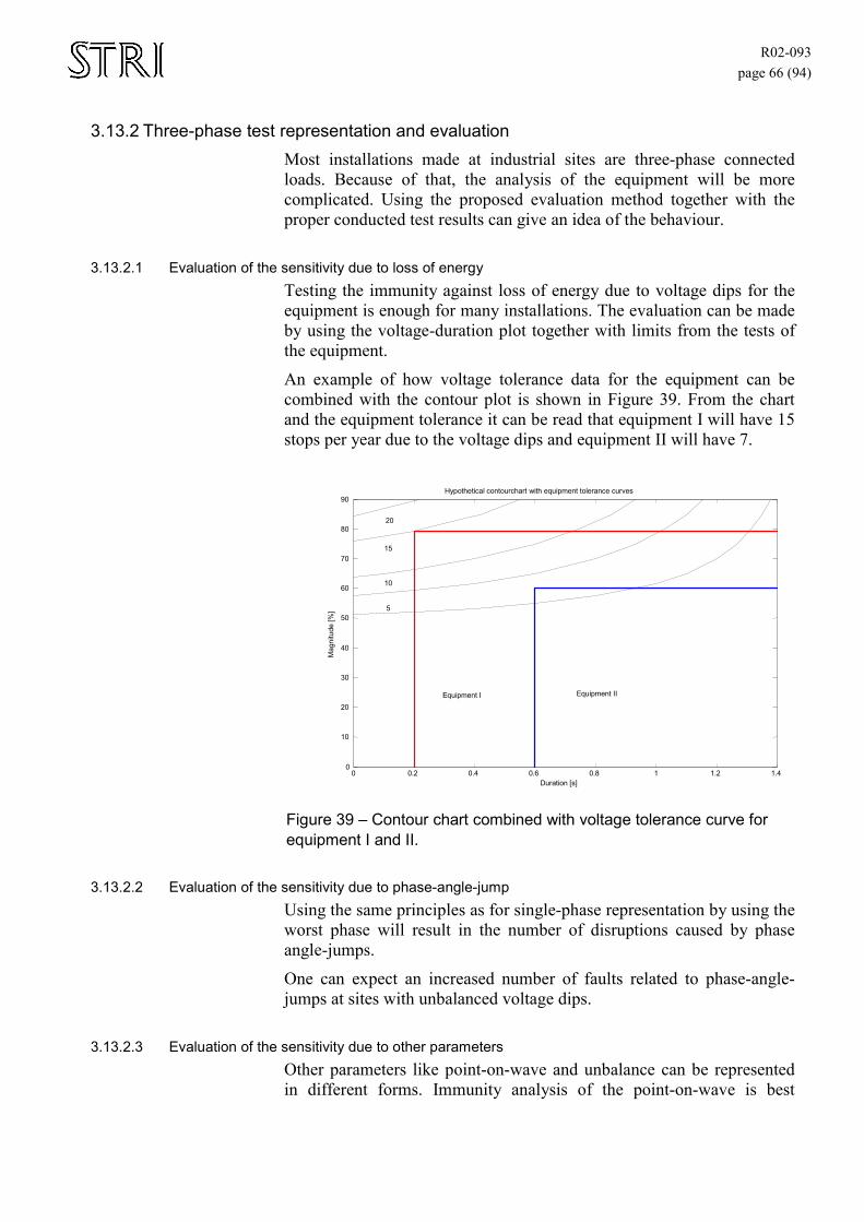
R02-093 page 66 (94)

3.13.2 Three-phase test representation and evaluation Most installations made at industrial sites are three-phase connected loads. Because of that, the analysis of the equipment will be more complicated. Using the proposed evaluation method together with the proper conducted test results can give an idea of the behaviour.

3.13.2.1 Evaluation of the sensitivity due to loss of energy Testing the immunity against loss of energy due to voltage dips for the equipment is enough for many installations. The evaluation can be made by using the voltage-duration plot together with limits from the tests of the equipment.

An example of how voltage tolerance data for the equipment can be combined with the contour plot is shown in Figure 39. From the chart and the equipment tolerance it can be read that equipment I will have 15 stops per year due to the voltage dips and equipment II will have 7.

0 0.2 0.4 0.6 0.8 1 1.2 1.4 0

10

20

30

40

50

60

70

80

90

5 10

15 20

Hypothetical contourchart with equipment tolerance curves

Duration [s]

Mag

nitu

de [%

]

Equipment I Equipment II

Figure 39 – Contour chart combined with voltage tolerance curve for equipment I and II.

3.13.2.2 Evaluation of the sensitivity due to phase-angle-jump Using the same principles as for single-phase representation by using the worst phase will result in the number of disruptions caused by phase angle-jumps.

One can expect an increased number of faults related to phase-angle-jumps at sites with unbalanced voltage dips.

3.13.2.3 Evaluation of the sensitivity due to other parameters Other parameters like point-on-wave and unbalance can be represented in different forms. Immunity analysis of the point-on-wave is best

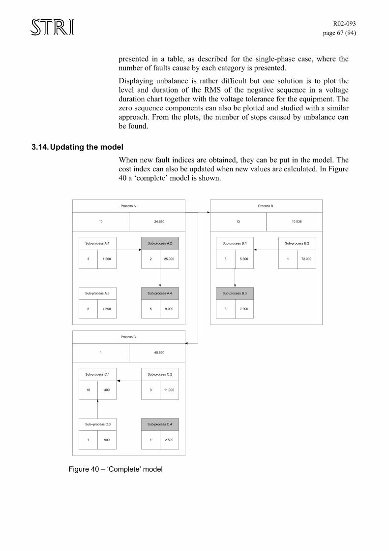
R02-093 page 67 (94)

presented in a table, as described for the single-phase case, where the number of faults cause by each category is presented.

Displaying unbalance is rather difficult but one solution is to plot the level and duration of the RMS of the negative sequence in a voltage duration chart together with the voltage tolerance for the equipment. The zero sequence components can also be plotted and studied with a similar approach. From the plots, the number of stops caused by unbalance can be found.

3.14. Updating the model When new fault indices are obtained, they can be put in the model. The cost index can also be updated when new values are calculated. In Figure 40 a ‘complete’ model is shown.

Sub-process A.1

1.500 3

Sub-process A.3

4.500 6

Sub-process A.2

25.000 2

Sub-process A.4

9.000 5

Sub-process B.1

5.300 8

Sub-process B.3

7.000 3

Sub-process B.2

72.000 1

Sub-process C.1

400 18

Sub--process C.3

900 1

Sub-process C.2

11.000 3

Sub-process C.4

2.500 1

Process C

45.520 1

Process A

24.650 10

Process B

10.938 13

Figure 40 – ‘Complete’ model

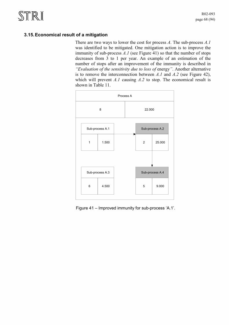
R02-093 page 68 (94)

3.15. Economical result of a mitigation There are two ways to lower the cost for process A. The sub-process A.1 was identified to be mitigated. One mitigation action is to improve the immunity of sub-process A.1 (see Figure 41) so that the number of stops decreases from 3 to 1 per year. An example of an estimation of the number of stops after an improvement of the immunity is described in “Evaluation of the sensitivity due to loss of energy”. Another alternative is to remove the interconnection between A.1 and A.2 (see Figure 42), which will prevent A.1 causing A.2 to stop. The economical result is shown in Table 11.

Sub-process A.1

1.500 1

Sub-process A.3

4.500 6

Sub-process A.2

25.000 2

Sub-process A.4

9.000 5

Process A

22.000 8

Figure 41 – Improved immunity for sub-process ‘A.1’.

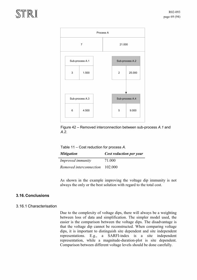
R02-093 page 69 (94)

Sub-process A.1

1.500 3

Sub-process A.3

4.500 6

Sub-process A.2

25.000 2

Sub-process A.4

9.000 5

Process A

21.000 7

Figure 42 – Removed interconnection between sub-process A.1 and A.2.

Table 11 – Cost reduction for process A.

Mitigation Cost reduction per year

Improved immunity 71.000

Removed interconnection 102.000

As shown in the example improving the voltage dip immunity is not always the only or the best solution with regard to the total cost.

3.16. Conclusions

3.16.1 Characterisation Due to the complexity of voltage dips, there will always be a weighting between loss of data and simplification. The simpler model used, the easier is the comparison between the voltage dips. The disadvantage is that the voltage dip cannot be reconstructed. When comparing voltage dips, it is important to distinguish site dependent and site independent representations. E.g., a SARFI-index is a site independent representation, while a magnitude-duration-plot is site dependent. Comparison between different voltage levels should be done carefully.

R02-093 page 70 (94)

3.16.2 Immunity determination of processes It is important to choose the right resolution for the study. A too detailed approach will cause too much work with too little result. However, a too rough approach will not be able to point out the right processes. The best approach is to start somewhere in the middle and then refine the model if necessary. Especially the cost index and the interlocking chart can be very time consuming.

To be able to obtain correct operational data it is important that everyone involved in fault clearing or operating the machinery is familiar with the fault reporting routines. It is also important that when there is a complete shutdown or large stop a proper investigation of sources and consequences is conducted.

The interlocking chart must be a dynamic model, which should be updated when new connections are discovered or changes are made to the system. It is reasonable to start with a rough model of the interlocking chart and then continuously improving it through time. It is important to try to divide the processes in such way that there are as few connections between the different processes as possible.

3.16.3 Testing It is important to perform tests for both the types of voltage dips that occur today, as well as for the ones that are likely to come. Knowledge of the equipment under test is very important to choose the right test methods and later on the proper evaluation.

Only using test standards available today is no guarantee that the test is thorough enough. It is more likely to be the opposite.

Before performing the test, an operating condition must be defined. The operating condition will tell if the equipment or process is working correctly during the voltage dip. Such conditions can be a constant torque, 10% speed variation, safe shutdown, etc.

3.16.4 Evaluation The evaluation of the test results will show which sub-process that causes most outages or the largest cost to the plant due to voltage dips. Depending of the values of the fault and cost index, the result will be either an index pointing out the sub-process, which is needed to take action on, or how much a sub-process contributes to lost revenue. This makes evaluation of different mitigation actions possible.

3.16.5 Mitigation It is not always the best solution to reduce the cost due to voltage dips by improving the immunity. The example shows that removing the interconnection between sub-process ‘A.1’ and ‘A.2’ reduced the cost with 102.000. Sometimes it is not possible to remove the interconnection

R02-093 page 71 (94)

between processes, but it is worth to consider before installing a lot of equipment to improve the voltage dip immunity.

R02-093 page 72 (94)

R02-093 page 73 (94)

4 Mitigation of voltage dips If the economical losses due to voltage dips are significant, mitigation actions can be profitable for the customer and even in some cases for the utility. Since there is no standard solution which will work for every site, each mitigation action must be carefully planned and evaluated.

There are different ways and responsibilities when trying to mitigate voltage dips. The utility can improve the reliability of the feeding grid, the end-user can improve the voltage supply inside the plant and the manufacture can improve the immunity level of the equipment. The right solution to chose is not obvious.

The best way to mitigate voltage dips is to coordinate the utility network and the equipment before a new plant is built.

4.1. Different perspectives and responsibilities There are different perspectives of voltage dip related problems between utilities, manufacturers of equipment and customers.

4.1.1 The utility The utility does not see the direct result or cost of voltage dips, but they have often knowledge about the cause and origin. They also have the possibility to perform mitigation actions at the origin of the voltage dip. In some cases, when the voltage dip occurs outside the local utility network it is almost impossible to find the cause of the voltage dip. However improving the grid reliability does not have to result in the same improved reliability for the plant. E.g. a utility can improve the grid reducing the outages but the number of dips remains the same. In that case the reliability of the utility will increase but for the plant the result is the same. The opposite is also possible if the utility decreases the number of dips but the downtime of the grid is not be affected.

4.1.2 The manufacturer The manufacturer has the possibilities and knowledge to build equipment with better ride-through capacity, without using batteries or UPS. The reasons why the manufacturers do not are many. One can be that customers are not willing to pay for increased immunity. Another factor can be that a better ride-through capability can be achieved with a decreased performance; torque, speed, etc., which the customer does not accept. It is also possible that the manufacturers do not really know what the customers need.

4.1.3 The customer The customer has very often a good knowledge of the consequences of a voltage dip, but seldom knows the origin of the disturbance. This makes mitigation actions harder for the customer. Further on mitigation actions

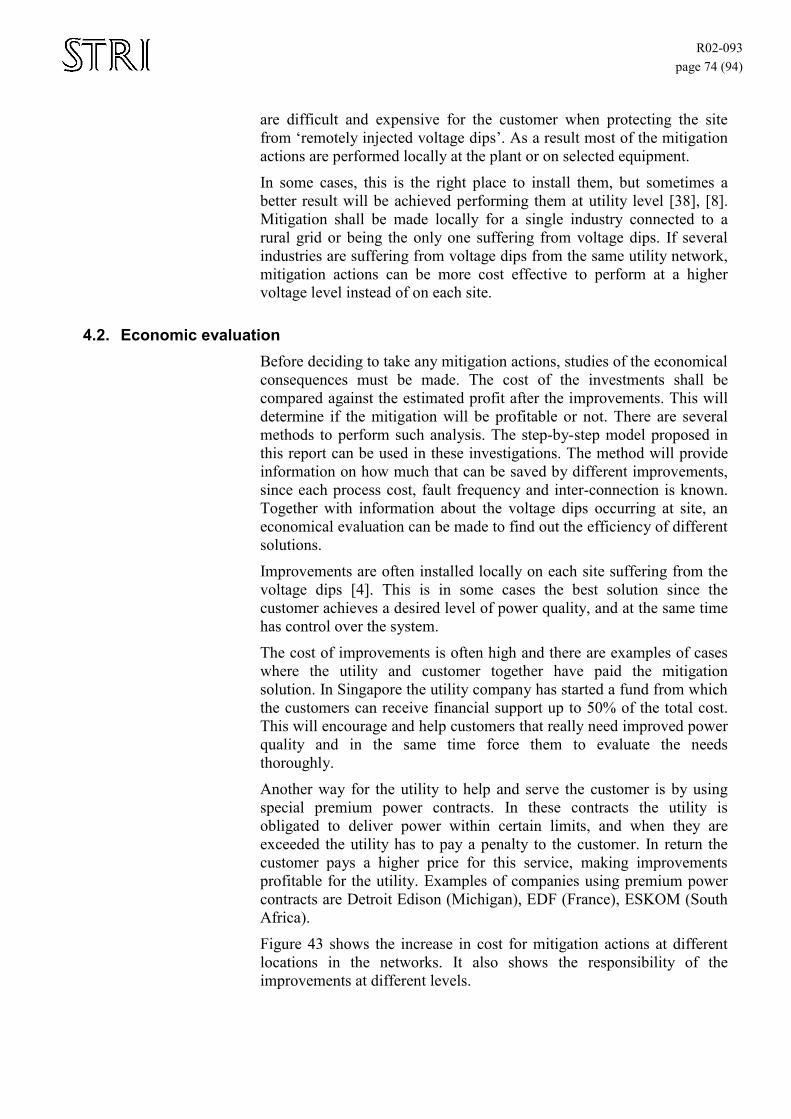
R02-093 page 74 (94)

are difficult and expensive for the customer when protecting the site from ‘remotely injected voltage dips’. As a result most of the mitigation actions are performed locally at the plant or on selected equipment.

In some cases, this is the right place to install them, but sometimes a better result will be achieved performing them at utility level [38], [8]. Mitigation shall be made locally for a single industry connected to a rural grid or being the only one suffering from voltage dips. If several industries are suffering from voltage dips from the same utility network, mitigation actions can be more cost effective to perform at a higher voltage level instead of on each site.

4.2. Economic evaluation Before deciding to take any mitigation actions, studies of the economical consequences must be made. The cost of the investments shall be compared against the estimated profit after the improvements. This will determine if the mitigation will be profitable or not. There are several methods to perform such analysis. The step-by-step model proposed in this report can be used in these investigations. The method will provide information on how much that can be saved by different improvements, since each process cost, fault frequency and inter-connection is known. Together with information about the voltage dips occurring at site, an economical evaluation can be made to find out the efficiency of different solutions.

Improvements are often installed locally on each site suffering from the voltage dips [4]. This is in some cases the best solution since the customer achieves a desired level of power quality, and at the same time has control over the system.

The cost of improvements is often high and there are examples of cases where the utility and customer together have paid the mitigation solution. In Singapore the utility company has started a fund from which the customers can receive financial support up to 50% of the total cost. This will encourage and help customers that really need improved power quality and in the same time force them to evaluate the needs thoroughly.

Another way for the utility to help and serve the customer is by using special premium power contracts. In these contracts the utility is obligated to deliver power within certain limits, and when they are exceeded the utility has to pay a penalty to the customer. In return the customer pays a higher price for this service, making improvements profitable for the utility. Examples of companies using premium power contracts are Detroit Edison (Michigan), EDF (France), ESKOM (South Africa).

Figure 43 shows the increase in cost for mitigation actions at different locations in the networks. It also shows the responsibility of the improvements at different levels.

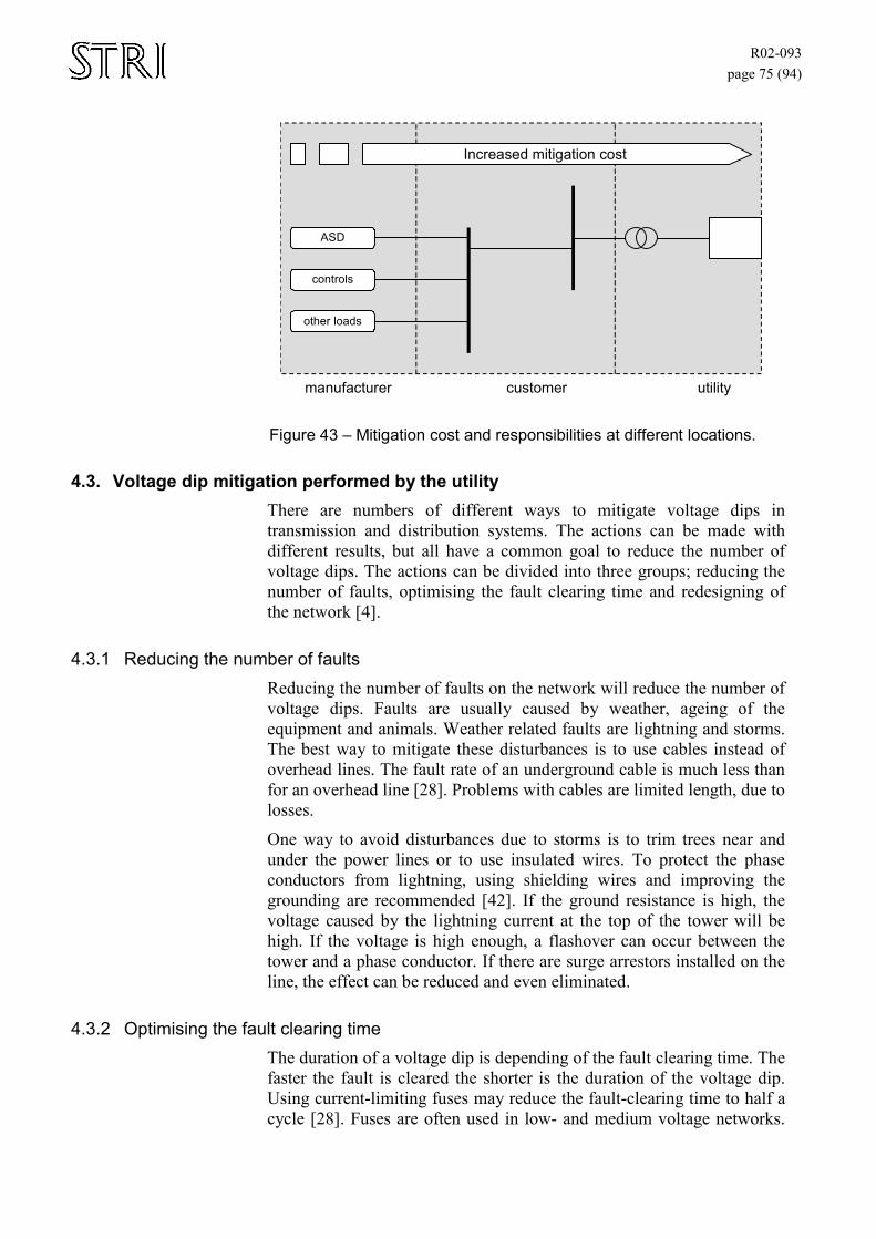
R02-093 page 75 (94)

manufacturer customer utility

ASD

controls

other loads

Increased mitigation cost

Figure 43 – Mitigation cost and responsibilities at different locations.

4.3. Voltage dip mitigation performed by the utility There are numbers of different ways to mitigate voltage dips in transmission and distribution systems. The actions can be made with different results, but all have a common goal to reduce the number of voltage dips. The actions can be divided into three groups; reducing the number of faults, optimising the fault clearing time and redesigning of the network [4].

4.3.1 Reducing the number of faults Reducing the number of faults on the network will reduce the number of voltage dips. Faults are usually caused by weather, ageing of the equipment and animals. Weather related faults are lightning and storms. The best way to mitigate these disturbances is to use cables instead of overhead lines. The fault rate of an underground cable is much less than for an overhead line [28]. Problems with cables are limited length, due to losses.

One way to avoid disturbances due to storms is to trim trees near and under the power lines or to use insulated wires. To protect the phase conductors from lightning, using shielding wires and improving the grounding are recommended [42]. If the ground resistance is high, the voltage caused by the lightning current at the top of the tower will be high. If the voltage is high enough, a flashover can occur between the tower and a phase conductor. If there are surge arrestors installed on the line, the effect can be reduced and even eliminated.

4.3.2 Optimising the fault clearing time The duration of a voltage dip is depending of the fault clearing time. The faster the fault is cleared the shorter is the duration of the voltage dip. Using current-limiting fuses may reduce the fault-clearing time to half a cycle [28]. Fuses are often used in low- and medium voltage networks.

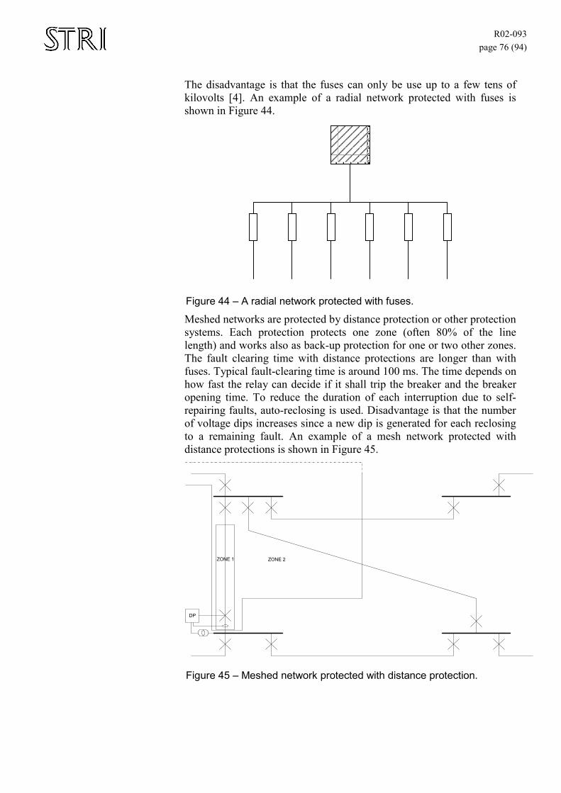
R02-093 page 76 (94)

The disadvantage is that the fuses can only be use up to a few tens of kilovolts [4]. An example of a radial network protected with fuses is shown in Figure 44.

Figure 44 – A radial network protected with fuses.

Meshed networks are protected by distance protection or other protection systems. Each protection protects one zone (often 80% of the line length) and works also as back-up protection for one or two other zones. The fault clearing time with distance protections are longer than with fuses. Typical fault-clearing time is around 100 ms. The time depends on how fast the relay can decide if it shall trip the breaker and the breaker opening time. To reduce the duration of each interruption due to self-repairing faults, auto-reclosing is used. Disadvantage is that the number of voltage dips increases since a new dip is generated for each reclosing to a remaining fault. An example of a mesh network protected with distance protections is shown in Figure 45.

DP

ZONE 1 ZONE 2

Figure 45 – Meshed network protected with distance protection.

R02-093 page 77 (94)

4.3.3 System design Radial networks are common in low- and medium voltage systems, with the advantage that simple protection schemes with fuses can be used. A disadvantage is the decreased availability due to longer interruptions. To improve the operation of the network the number of feeders fed from the same substation can be reduced. To further improve the supply to sensitive loads, parallel feeders from two different substations or busbars can be used. The disadvantage is that the impedance during a fault becomes less, and the severity of the voltage dip increases. Using current-limiting fuses or reactors in all the non-prioritised feeders will limit the propagation of the voltage dip during a fault [4].

4.4. Improvements of the equipment immunity performed by the manufacturer Different strategies can be used when improving the immunity of various equipments.

4.4.1 Single-phase rectifier loads Computers, PLC and other small single-phase equipment with rectifiers, usually have a capacitor as energy storage. Considerations are normally not made to voltage dips when choosing values of the capacitance, since it is not an issue raised by the customers and it will increase the cost. Instead the designer focuses on minimizing it. They normally use the lowest expected voltage and the maximum expected load as limits. To make the equipment ride-through one cycle, the capacitance must at least be doubled. To withstand 1s. it must be 100 times larger [38]. The cost of increasing the capacitor 100 times is probably much lower than redesigning the network.

4.4.2 Three-phase loads Improving the voltage dip immunity of different three-phase equipment with converters or rectifiers mainly consists of three actions; improving the energy storage capacity, the control design or the operation criterias.

Adding more capacitance to the DC-link improves the storage capacity. Such improvement shows good result against single-phase and two-phase voltage dips. Against three-phase voltage dips the solution is not very effective [28].

Another way to improve the ride-through capability is by designing the DC/DC or AC/DC rectifier to operate with a varying input voltage. It is generally harder to improve a DC adjustable speed drive system because of the fast drop of armature-current.

A third possibility to improve the ride-trough of adjustable drives is to let the torque vary during the voltage dip. Tuning the under-voltage and over-current protection to the limits of what the machine can withstand, is another option to improve the immunity. It requires knowledge of the

R02-093 page 78 (94)

process and shall therefore be done on site. Very often it is only the manufacturer who tunes the systems on site.

4.4.3 Directly fed induction machines Induction machines connected directly to the network will work as generators during the voltage dip. When the voltage recovers, they will draw a large inrush-current, which can aggravate the situation, especially when many motors start at the same time [38].

Adding controllers to the machines, which lets them contribute to the mitigation and then soft start them with different time delays, can avoid some problems.

4.4.4 Other equipment Other equipment like relays, contactors and sensors can also be improved by using coil-locks to ride-through the voltage dip [8]. Sensors can be designed to hold their value during a voltage dip. Improved checking of realistic data in control algorithm can be implemented to prevent the use of faulted values caused by the voltage dip.

4.5. Local mitigation actions performed by the customer Most of the mitigation solutions today are done locally at site or on selected equipment [28]. One reasons is that this is the only part in the chain of power delivery where the customer can have a complete overview. The fact that costs for mitigation actions in higher voltage levels are often higher is also on important reason [38]. Performing mitigation at site makes it possible for the customer to only protect the disturbed equipment.

4.5.1 On site generation and prioritised busbars One way to establish a higher immunity for a site is to have power generation within the plant. There will not only be an advantage of improved immunity during the voltage dips. Some industries, with steam production within the plant, can even find it profitable to use it for electric generation. Generally, the locally generated power is not enough to supply the whole site in a complete island operation, and therefore other solutions must be made.

Instead of supporting all loads, they are divided into prioritised and non-prioritised loads. The different types are then connected to different busbars at the site as shown in Figure 46. The busbars are often connected via a closed circuit breaker. When a disturbance is expected the prioritised busbar is disconnected from the main grid and only supplied by the local generation.

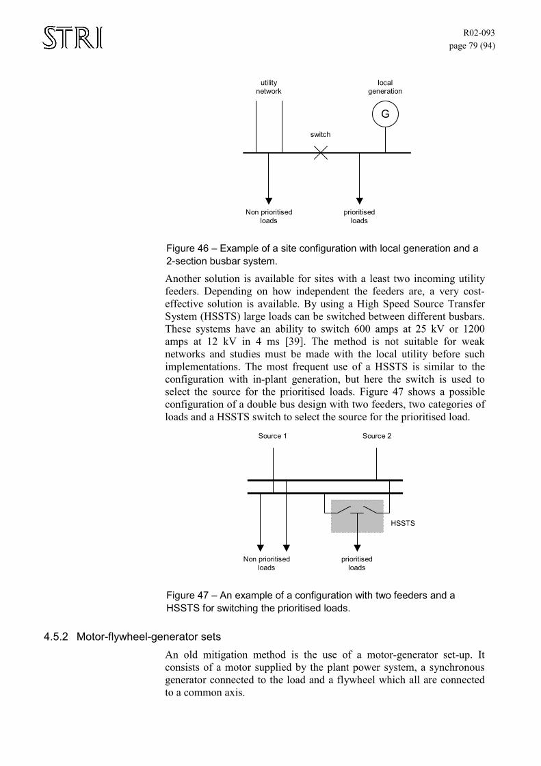
R02-093 page 79 (94)

G

utility network

Non prioritised loads

local generation

prioritised loads

switch

Figure 46 – Example of a site configuration with local generation and a 2-section busbar system.

Another solution is available for sites with a least two incoming utility feeders. Depending on how independent the feeders are, a very cost-effective solution is available. By using a High Speed Source Transfer System (HSSTS) large loads can be switched between different busbars. These systems have an ability to switch 600 amps at 25 kV or 1200 amps at 12 kV in 4 ms [39]. The method is not suitable for weak networks and studies must be made with the local utility before such implementations. The most frequent use of a HSSTS is similar to the configuration with in-plant generation, but here the switch is used to select the source for the prioritised loads. Figure 47 shows a possible configuration of a double bus design with two feeders, two categories of loads and a HSSTS switch to select the source for the prioritised load.

Source 1

Non prioritised loads

HSSTS

prioritised loads

Source 2

Figure 47 – An example of a configuration with two feeders and a HSSTS for switching the prioritised loads.

4.5.2 Motor-flywheel-generator sets An old mitigation method is the use of a motor-generator set-up. It consists of a motor supplied by the plant power system, a synchronous generator connected to the load and a flywheel which all are connected to a common axis.

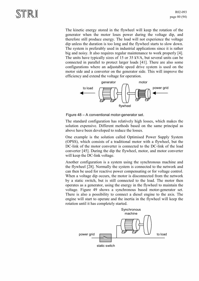
R02-093 page 80 (94)

The kinetic energy stored in the flywheel will keep the rotation of the generator when the motor loses power during the voltage dip, and therefore still produce energy. The load will not experience the voltage dip unless the duration is too long and the flywheel starts to slow down. The system is preferably used in industrial applications since it is rather big and noisy. It also requires regular maintenance to work properly [4]. The units have typically sizes of 15 or 35 kVA, but several units can be connected in parallel to protect larger loads [41]. There are also some configurations where an adjustable speed drive system is used on the motor side and a converter on the generator side. This will improve the efficiency and extend the voltage for operation.

generator

flywheel

motor

to load power grid

Figure 48 – A conventional motor-generator set.

The standard configuration has relatively high losses, which makes the solution expensive. Different methods based on the same principal as above have been developed to reduce the losses.

One example is the solution called Optimised Power Supply System (OPSS), which consists of a traditional motor with a flywheel, but the DC-link of the motor converter is connected to the DC-link of the load converter [45]. During the dip the flywheel, motor, and motor converter will keep the DC-link voltage.

Another configuration is a system using the synchronous machine and the flywheel [28]. Normally the system is connected to the network and can then be used for reactive power compensating or for voltage control. When a voltage dip occurs, the motor is disconnected from the network by a static switch, but is still connected to the load. The motor then operates as a generator, using the energy in the flywheel to maintain the voltage. Figure 49 shows a synchronous based motor-generator set. There is also a possibility to connect a diesel engine to the axis. The engine will start to operate and the inertia in the flywheel will keep the rotation until it has completely started.

Synchronous machine

to load power grid

static switch

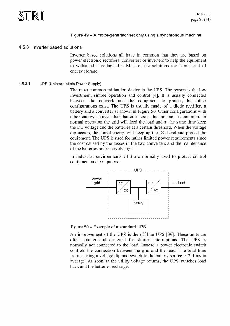
R02-093 page 81 (94)

Figure 49 – A motor-generator set only using a synchronous machine.

4.5.3 Inverter based solutions Inverter based solutions all have in common that they are based on power electronic rectifiers, converters or inverters to help the equipment to withstand a voltage dip. Most of the solutions use some kind of energy storage.

4.5.3.1 UPS (Uninterruptible Power Supply) The most common mitigation device is the UPS. The reason is the low investment, simple operation and control [4]. It is usually connected between the network and the equipment to protect, but other configurations exist. The UPS is usually made of a diode rectifier, a battery and a converter as shown in Figure 50. Other configurations with other energy sources than batteries exist, but are not as common. In normal operation the grid will feed the load and at the same time keep the DC voltage and the batteries at a certain threshold. When the voltage dip occurs, the stored energy will keep up the DC level and protect the equipment. The UPS is used for rather limited power requirements since the cost caused by the losses in the two converters and the maintenance of the batteries are relatively high.

In industrial environments UPS are normally used to protect control equipment and computers.

DC

AC

battery

AC

DC

UPS

to load power grid

Figure 50 – Example of a standard UPS

An improvement of the UPS is the off-line UPS [39]. These units are often smaller and designed for shorter interruptions. The UPS is normally not connected to the load. Instead a power electronic switch controls the connection between the grid and the load. The total time from sensing a voltage dip and switch to the battery source is 2-4 ms in average. As soon as the utility voltage returns, the UPS switches load back and the batteries recharge.

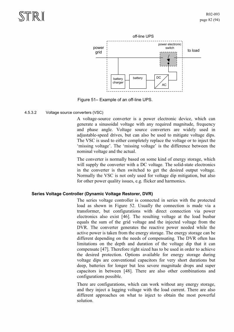
R02-093 page 82 (94)

battery charger

battery

off-line UPS

to load power grid

AC

DC

power electronic switch

Figure 51– Example of an off-line UPS.

4.5.3.2 Voltage source converters (VSC) A voltage-source converter is a power electronic device, which can generate a sinusoidal voltage with any required magnitude, frequency and phase angle. Voltage source converters are widely used in adjustable-speed drives, but can also be used to mitigate voltage dips. The VSC is used to either completely replace the voltage or to inject the ‘missing voltage’. The ‘missing voltage’ is the difference between the nominal voltage and the actual.

The converter is normally based on some kind of energy storage, which will supply the converter with a DC voltage. The solid-state electronics in the converter is then switched to get the desired output voltage. Normally the VSC is not only used for voltage dip mitigation, but also for other power quality issues, e.g. flicker and harmonics.

Series Voltage Controller (Dynamic Voltage Restorer, DVR) The series voltage controller is connected in series with the protected load as shown in Figure 52. Usually the connection is made via a transformer, but configurations with direct connection via power electronics also exist [46]. The resulting voltage at the load busbar equals the sum of the grid voltage and the injected voltage from the DVR. The converter generates the reactive power needed while the active power is taken from the energy storage. The energy storage can be different depending on the needs of compensating. The DVR often has limitations on the depth and duration of the voltage dip that it can compensate [47]. Therefore right sized has to be used in order to achieve the desired protection. Options available for energy storage during voltage dips are conventional capacitors for very short durations but deep, batteries for longer but less severe magnitude drops and super capacitors in between [48]. There are also other combinations and configurations possible.

There are configurations, which can work without any energy storage, and they inject a lagging voltage with the load current. There are also different approaches on what to inject to obtain the most powerful solution.

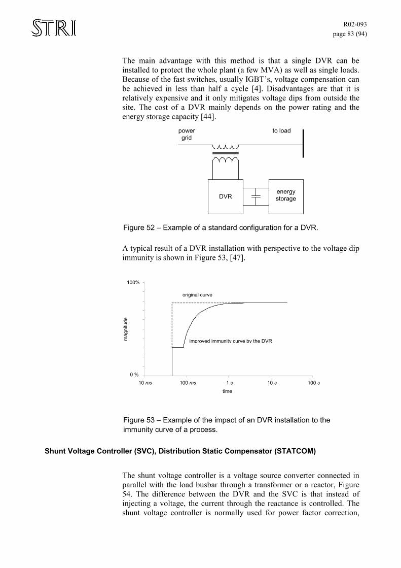
R02-093 page 83 (94)

The main advantage with this method is that a single DVR can be installed to protect the whole plant (a few MVA) as well as single loads. Because of the fast switches, usually IGBT’s, voltage compensation can be achieved in less than half a cycle [4]. Disadvantages are that it is relatively expensive and it only mitigates voltage dips from outside the site. The cost of a DVR mainly depends on the power rating and the energy storage capacity [44].

DVR

energy storage

power grid

to load

Figure 52 – Example of a standard configuration for a DVR.

A typical result of a DVR installation with perspective to the voltage dip immunity is shown in Figure 53, [47].

0 %

100%

10 ms 100 ms 1 s 10 s 100 s time

mag

nitu

de

improved immunity curve by the DVR

original curve

Figure 53 – Example of the impact of an DVR installation to the immunity curve of a process.

Shunt Voltage Controller (SVC), Distribution Static Compensator (STATCOM)

The shunt voltage controller is a voltage source converter connected in parallel with the load busbar through a transformer or a reactor, Figure 54. The difference between the DVR and the SVC is that instead of injecting a voltage, the current through the reactance is controlled. The shunt voltage controller is normally used for power factor correction,

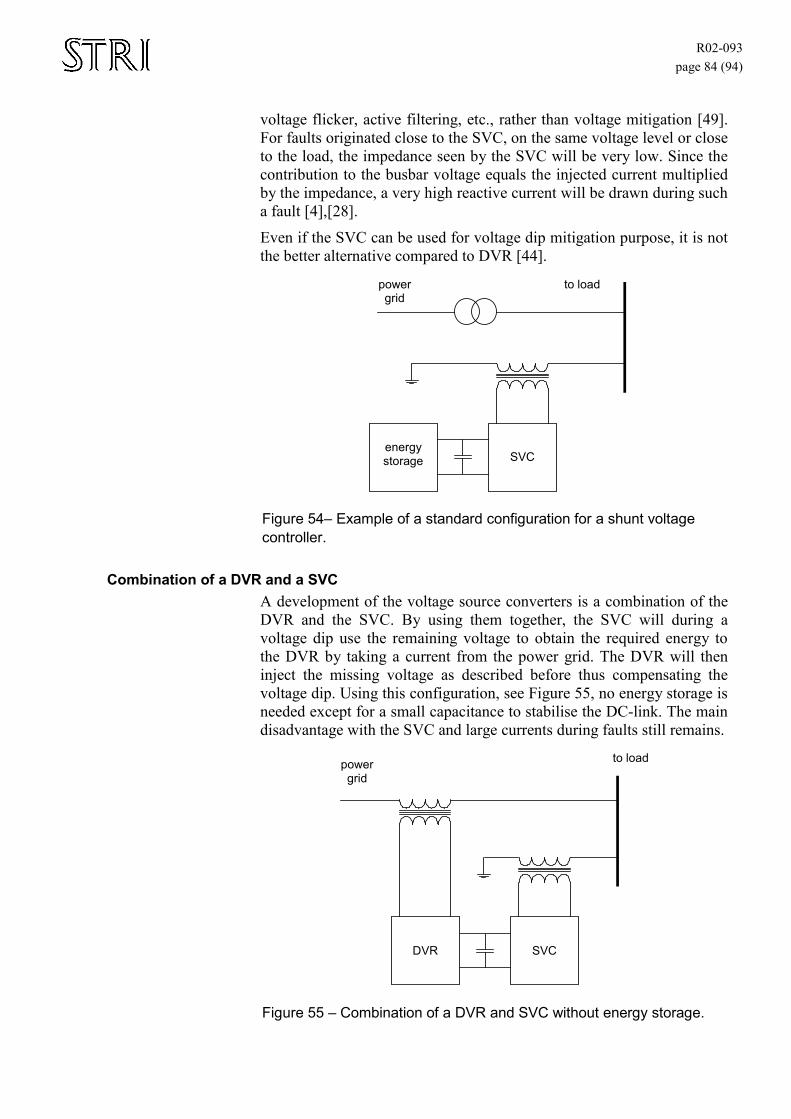
R02-093 page 84 (94)

voltage flicker, active filtering, etc., rather than voltage mitigation [49]. For faults originated close to the SVC, on the same voltage level or close to the load, the impedance seen by the SVC will be very low. Since the contribution to the busbar voltage equals the injected current multiplied by the impedance, a very high reactive current will be drawn during such a fault [4],[28].

Even if the SVC can be used for voltage dip mitigation purpose, it is not the better alternative compared to DVR [44].

SVC

energy storage

power grid

to load

Figure 54– Example of a standard configuration for a shunt voltage controller.

Combination of a DVR and a SVC A development of the voltage source converters is a combination of the DVR and the SVC. By using them together, the SVC will during a voltage dip use the remaining voltage to obtain the required energy to the DVR by taking a current from the power grid. The DVR will then inject the missing voltage as described before thus compensating the voltage dip. Using this configuration, see Figure 55, no energy storage is needed except for a small capacitance to stabilise the DC-link. The main disadvantage with the SVC and large currents during faults still remains.

SVC

DVR

power grid

to load

Figure 55 – Combination of a DVR and SVC without energy storage.

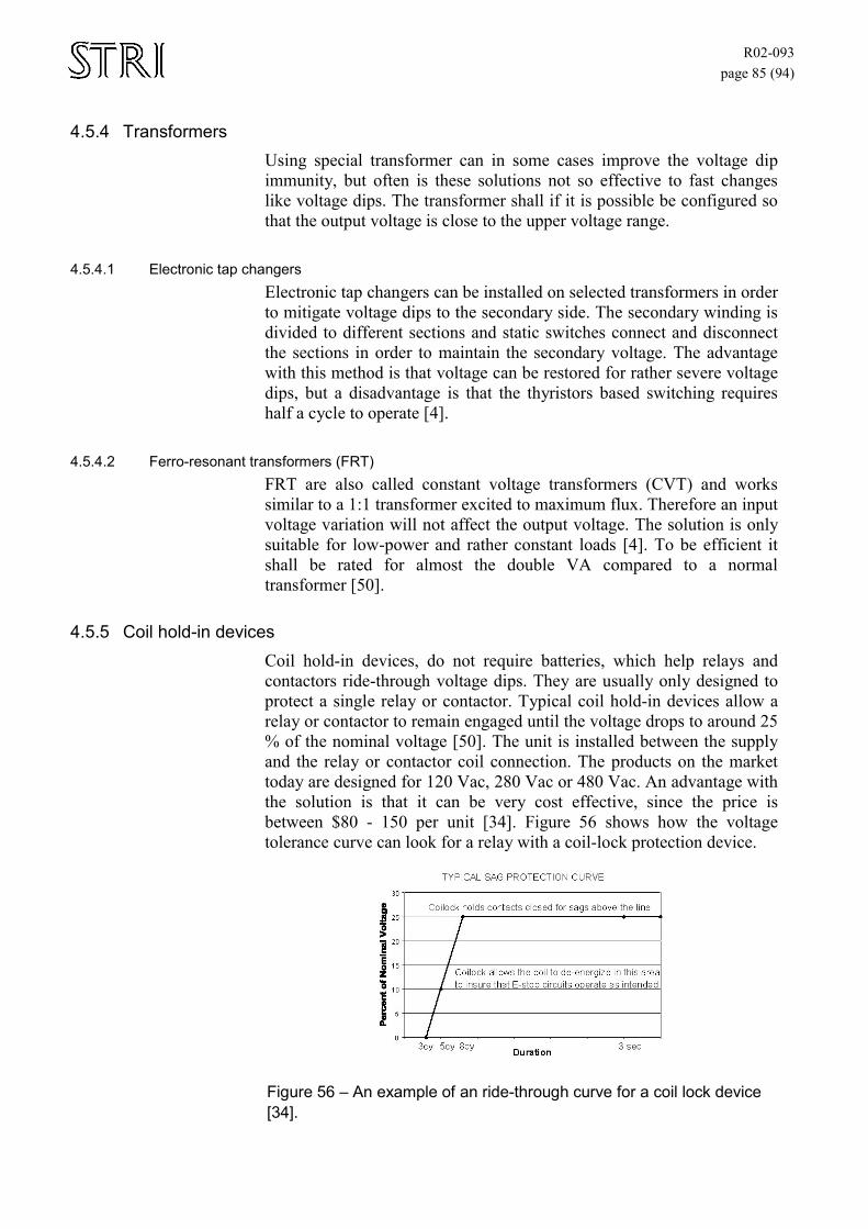
R02-093 page 85 (94)

4.5.4 Transformers Using special transformer can in some cases improve the voltage dip immunity, but often is these solutions not so effective to fast changes like voltage dips. The transformer shall if it is possible be configured so that the output voltage is close to the upper voltage range.

4.5.4.1 Electronic tap changers Electronic tap changers can be installed on selected transformers in order to mitigate voltage dips to the secondary side. The secondary winding is divided to different sections and static switches connect and disconnect the sections in order to maintain the secondary voltage. The advantage with this method is that voltage can be restored for rather severe voltage dips, but a disadvantage is that the thyristors based switching requires half a cycle to operate [4].

4.5.4.2 Ferro-resonant transformers (FRT) FRT are also called constant voltage transformers (CVT) and works similar to a 1:1 transformer excited to maximum flux. Therefore an input voltage variation will not affect the output voltage. The solution is only suitable for low-power and rather constant loads [4]. To be efficient it shall be rated for almost the double VA compared to a normal transformer [50].

4.5.5 Coil hold-in devices Coil hold-in devices, do not require batteries, which help relays and contactors ride-through voltage dips. They are usually only designed to protect a single relay or contactor. Typical coil hold-in devices allow a relay or contactor to remain engaged until the voltage drops to around 25 % of the nominal voltage [50]. The unit is installed between the supply and the relay or contactor coil connection. The products on the market today are designed for 120 Vac, 280 Vac or 480 Vac. An advantage with the solution is that it can be very cost effective, since the price is between $80 - 150 per unit [34]. Figure 56 shows how the voltage tolerance curve can look for a relay with a coil-lock protection device.

Figure 56 – An example of an ride-through curve for a coil lock device [34].

R02-093 page 86 (94)

4.6. Energy storage The energy required during a disturbance through voltage source converters; rectifiers, inverters, UPS, can be stored electrically, kinetically, chemically, or magnetically. These can be implemented by capacitors, flywheels, batteries or superconducting magnetic coils (SMES). The development of new storage medium results in increased capability of those devices [41].

4.6.1 Capacitors Capacitors can be used as energy storage to produce active power. The amount of energy stored on the capacitor is proportional to the square of the voltage. To supply a constant dc-voltage there must be a dc-dc-converter to regulate the voltage, since the capacitor voltage decreases when the capacitor is discharged. Capacitors can normally be used up to a few seconds ride-through [28], depending on the load.

4.6.2 Batteries Batteries have a higher energy density than capacitors and supply power for a longer time than capacitors, but at a slower rate. Batteries have a few disadvantages compared to capacitors; they may contain substances, which are not environmentally friendly, a limited lifetime, and they require maintenance to operate as intended [28].

4.6.3 Superconducting magnetic coils To deliver a high peak-power, e.g. an interruption in a large industrial system, superconducting magnetic coils are recommended in [40]. The energy is stored in the magnetic field, generated by a DC current. The conductor is generally a niobium-titanium alloy, is kept at liquid helium temperature in order to be superconducting [40]. The energy can be stored in a persistent mode until required. The advantages with a SMES are that it requires less space than an energy storage medium and that the price can compete with UPS in the kVA range [41].

4.7. Conclusions

4.7.1 Everything depends on the economics Dealing with voltage dips is, in addition to a technical problem, also an economical issue. If the cost for solutions is less then the disturbance cost then there exist an incentive to implement them. In other cases the mitigation actions will not improve the economical result and are more difficult to motivate. An important question is who shall pay for the mitigation and the improved power quality? One way, the Singapore Power is using a practice, where the utility and customer split the cost. Even better is when the customer and the utility work together towards the manufacturers and specify a certain immunity level for him to reach.

R02-093 page 87 (94)

They may for instant require that the equipment has to comply with the SEMI F47 standard.

4.7.2 Customer oriented approach Whenever dealing with voltage dips as a problem, a customer perspective must be used, since he is the one suffering from them. Utilities and manufacturers must always try to understand the customer needs. Singapore power Ltd. has been working with a model, to some extent similar with the model presented in this report. In their model, they have a very high customer focus [26].

4.7.3 Where shall the dips problem be solved? Careful analysis shall be made before every mitigation action is taken. The location of the solution, at the utility, in a complete plant or at a single component, shall be considered. In some cases, e.g. an industrial campus with high tech industries, a mitigation action done by the utility can be more cost effective then many separate actions at each site. If the utility can offer such power quality solutions, then he can sign special power contracts with the customers to get some of the investments back. In other cases, e.g. for a single customer, a locally placed solution can be a better alternative.

4.7.4 Choice of solutions It is not always obvious that the best solution is to improve the equipment immunity. Other improvements, for example increasing a buffer between two machines, or using separately power supplies to them must also be considered. As shown in the example in “Chapter 3, Economical result of a mitigation” earlier, a changed interconnection between processes can result in a large amount of money being saved.

However, in many cases, voltage dip mitigation will be the chosen method and then the correct solution shall be implemented. The choice shall be based on carefully conducted studies and analysis. If it is possible, UPS or other energy storage methods using batteries shall be avoided in heavy industries and in large numbers. This is because they require regular maintenance and are therefore sometimes unreliable. It is also very important not to install larger capacity than needed to ride-through the dips.

R02-093 page 88 (94)

R02-093 page 89 (94)

References [1] J. V. Milanović, “Characteristics of voltage sags in radial

networks with dynamic loads and embedded generators,” in Power tech proceedings, 2001 IEEE Porto, 2001, p. 6 pp. vol.1, ISBN 0780371399.

[2] G. Yaleinkaya, M.H.J. Bollen, P.A. Crossley, ” Characterization of voltage sags in industrial distribution systems,” IEEE transactions on industry applications, vol. 34, no. 4, July/August, pp. 682-688, 1998, ISSN 00939994.

[3] M.H.J. Bollen, ”Comparing voltage dip survey results,” Power Engineering Society Winter Meeting, 2002. IEEE Volume: 2, pp.1131-1134, 2002

[4] Sannino, M.G. Miller, M.J.H. Bollen, “ Overview of voltage sag mitigation,“ Power Engineering Society Winter Meeting, 2002. IEEE, Volume: 4, pp. 2872-2878, 2002

[5] P.K. Lim, D.S. Dorr, “Understanding and resolving voltage sag related problems for sensitive industrial customers,” in 2000 IEEE power engineering society winter meeting, pp. 2886-2890, 2000, ISBN 0780359356.

[6] R.S. Thallm, G.T. Heydt, “Power acceptability and voltage sag indices in the three phase sense,” Power Engineering Society Summer Meeting, 2000. IEEE, Volume: 2, pp. 905-910, 2000

[7] J. Lamoree, D. Mueller, P. Vinett, W. Jones, M. Samotyj, ” Voltage sag analysis case studies,” IEEE transactions on industry applications, vol. 30, no. 4, July/August, pp.1083-1089, 1994, ISSN 00939994.

[8] S.T. Chang, K.Y. Chua, C.C. Slew, T.L. Tan, ” Power quality initiative in Singapore,” Electric Distribution, 2001. Part 1: Contributions. CIRED. 16th International Conference and Exhibition on (IEEE Conf. Publ No. 482), Volume: 2, 2001

[9] E. Lakervi, “Voltage sag mitigation through distribution system design,“ in IEEE power engineering society winter meeting 2000, 2000, pp. 2879 -2880 vol.4, ISBN 0780359356.

[10] B.M. Nacke, R.L. Schlake, “The importance of power quality management in the pulp and paper industry”, IEEE transactions on industry applications, vol. 38, no. 3, May/June, 758-762, 2002, ISSN 00939994.

[11] Alves M.F., Ribeiro T.N. “Voltage sag: an overview of IEC and IEEE standards and application criteria”, Transmission

R02-093 page 90 (94)

and Distribution Conference, 1999 IEEE , Volume: 2 , 1999 pp. 585 -589 vol.2

[12] Shih-An Yin, Chan-Nan Lu, E. Liu, Yu-Chang Huang, Chinug-Yi “Huang, A survey on high tech industry power quality requirements,” in 2001 IEEE/PES transmission and distribution conference and exposition, 2001, pp. 548-553, ISBN 0780372859.

[13] Collins E.R., Zapardiel F., “An experimental assessment of AC contactor behavior during voltage sags”, Industrial Electronics, 1997. ISIE '97., Proceedings of the IEEE International Symposium on , Volume: 2, 1997 pp. 439 -444 vol.2

[14] Langley R., Mansoor A., Collins E.R., Jr., Morgan R.L. ,“Voltage sag ride-through testing of adjustable speed drives using a controllable dynamic dynamometer “, Harmonics and Quality of Power Proceedings, 1998. Proceedings. 8th International Conference On, Volume: 1, 1998, pp. 566 -571 vol.1

[15] Bollen M.H.J., Zhang L.D., “Analysis of voltage tolerance of AC adjustable-speed drives for three-phase balanced and unbalanced sags”, IEEE Transactions on Industry Applications, Volume: 36 Issue: 3, May-June 2000, pp. 904 –910

[16] Keus A.K., Abrahams R., Van Coller J.M., Koch R.G., ”Analysis of voltage dip (sag) testing results of a 15 kW PWM adjustable speed drive (ASD) “, Electric Machines and Drives, 1999. International Conference IEMD '99 , 1999, pp. 213 -215

[17] E.R.Jr. Collins, M.A. Bridgwood, “The impact of power system disturbances on AC-coil contactors”, in IEEE 1997 annual textile, fiber, and film industry technical conference, 1997, pp. 2-6, ISBN 0780340906.

[18] F. Carlsson, B. Widell, C. Sadarangani, ” Ride-through investigations for a hot rolling mill process,” in PowerCon 2000 International Conference on Power System Technology, 2000, pp. 1605 -1608 vol.3, ISBN 0780363388.

[19] E. Agneholm, J.E. Daalder, ”Load recovery in the pulp and paper industry following a disturbance,” IEEE Transactions on Power Systems, vol. 15 ,Issue 2, 2000, pp. 831–837, ISSN 08858950.

[20] J.L. Duran-Gomez, P.N. Enjeti, Byeong Ok Woo, ” Effect of voltage sags on adjustable-speed drives: a critical evaluation and an approach to improve performance,” IEEE Transactions on Industry Applications, vol. 35, no. 6 Nov./Dec., pp.1440-1449, ISSN 00939994.

R02-093 page 91 (94)

[21] M.H.J. Bollen, ”The influence of motor reacceleration on voltage sags,” IEEE Transactions on Industry Applications, vol. 31, no. 4 Jul/Aug, pp. 667 –674, ISSN 00939994.

[22] J.C. Gomez, M.M. Morcos, C. Reineri, G. Campetelli, “Induction motor behavior under short interruptions and voltage sags,” IEEE Power Engineering Review, February, pp. 11-15, 2001, ISSN 02721724

[23] L. Guasch, F. Corcoles, J. Pedra, ” Effects of unsymmetrical voltage sag types E, F and G on induction motors,” in Ninth International Conference on Harmonics and Quality of Power, 2002, pp 796 –803 vol. 3, ISBN 0780364996

[24] D.S. Dorr, A. Mansoor, A.G. Morinec, J.C. Worley, “Effects of power line voltage variations on different types of 400-W high-pressure sodium ballasts,” IEEE Transactions on Industry Applications, vol. 33, no. 2, March/April, pp 472 –476, 1997, ISSN 00939994

[25] E.R. Collins, Jr., A. Mansoor, “Effects of voltage sags on AC motor drives,” in IEEE 1997 Annual Textile, Fiber, and Film Industry Technical Conference, 1997, 7 p, ISBN 0780340906

[26] Ronghua G.R., Suan H.C, “A customer - oriented approach in managing power quality in Singapore”, International Power Quality Conference IPQC 2002, Oct 2002, pp. 188-192 vol 2.

[27] Pumar, J. Amantegui, J.R. Torrealday, C. Ugarte, ”A comparison between d.c. and a.c. drives as regards their behaviour in the presence of voltage dips: new techniques for reducing the susceptibility of a.c. drives,” Electricity Distribution. Part 1: Contributions. CIRED. 14th International Conference and Exhibition on (IEE Conf. Publ. No. 438), 1997, pp 2.9.1-2.9.5, ISBN 0852966741

[28] M.H.J, Bollen, “Understanding power quality problems,” P.M. Anderson, 2000, New York, IEEE Press, ISBN 0-7803-4713-7

[29] Boldea, Syed A. Nasar, “The Induction Machine Handbook,” 1st edition , n.p., CRC Press, December 15, 2001, ISBN: 0849300045;

[30] Das, J.C., ”Effects of momentary voltage dips on the operation of induction and synchronous motors”, Industry Applications, IEEE Transactions on , Volume: 26 Issue: 4 , July-Aug. 1990, pp. 711 -718

[31] Michaels K.M., ”Sensible approaches to diagnosing power quality problems”, IEEE Transactions on Industry

R02-093 page 92 (94)

Applications, Volume: 33 Issue: 4 , July-Aug. 1997, pp. 1124 –1130

[32] M.F. McGranaghan, D.R. Mueller, M.J. Samotyj, ”Voltage sags in industrial systems,” IEEE Trans. Ind. Applic. 29 (2), pp. 397-403, 1993

[33] H.G. Sarmiento, E. Estrada,” A voltage sag study in an industry with adjustable speed drives,” in Industrial and Commercial Power Systems Technical Conference, 1994, pp 85-89, ISBN 0780318773

[34] Power Quality Solutions, ” COIL-LOCK™ HOLD-IN DEVICE” [Online document], [2002 Nov. 5], Available at http://www.pqsi.com/Coilock%20Brochure%2012-2001.pdf

[35] Bollen H.H.J, “Ongoing standard work on statistical presentation of voltage dips.” Draft of article, July 2002.

[36] N. Mohan, T.M. Undeland, W.P Robbins, Power electronics – Converters, applications and design, second edition, John Wiley and sons, New York, 1995

[37] ”ITI (CBEMA) curve application note,” [Online document], [2002 Jun. 25], Available at http://www.itic.org

[38] Chapman, ” Power quality application guide – Voltage voltage dips,” [Online document], (Nov. 2001), [2002 Oct. 15], Available at http://www.cda.org.uk/megab2/elecapps/pub501/ 51_lo_R2.pdf

[39] B.P Roberts, “Power quality solution alternatives for low and medium voltage continuous processloads,” Rural Electric Power Conference, 2002 IEEE , 2002, pp. C4 -1-7

[40] P. Esterban, A. Bautista, J.L. Gutiérrez-Iglesias, J.M. Rodriguez, E. Urretavizcaya, “SMES system applications to improve quality service,” CIRED, 1997, Conference publication no. 438, pp. 2.12.1-2.12.4

[41] Braz, P. Hofmann, R. Mauro, C.J. Mellhorn, ”An evaluation of energy storage techniques for improving ride-through capability for sensitive customers on underground networks,” 1996, pp. 55-64

[42] Dettloff A., Sabin D., “Power quality performance component of the special manufacturing contracts between power provider and customer”, Proceedings. Ninth International Conference on Harmonics and Quality of Power, 2000, Volume: 2, pp. 416 -424 vol.2

[43] Johns, M., Morgan, L, “Voltage sag mitigation through ridethrough coordination”, Technical Conference Textile, Fiber and Film Industry, 1994, IEEE 1994, Annual , pp. 1 –5

R02-093 page 93 (94)

[44] Haque M.H, Vilathgamuwa D.M et al., “Voltage sag correction by DSTATCOM and DVR”, International Power Quality Conference IPQC 2002, Oct 2002, pp. 261-272 vol 1.

[45] Widodo K, Peng O.P., “Optimized Power Supply System (OPSS)”, International Power Quality Conference IPQC 2002, Oct 2002, pp. 767-775 vol 2.

[46] Vilathgamuwa D.M, Wijekoon H.M., “Analysis and control of transformerless Dynamic Voltage Restorer for compensating long duration voltage sags”, International Power Quality Conference IPQC 2002, Oct 2002, pp. 755-766 vol 2.

[47] Er C.S, Chang C.S., Chan E.K., Au B.S., Kerk S.G., “Voltage dip assessment via power quality monitoring”, International Power Quality Conference IPQC 2002, Oct 2002, pp. 491-498 vol 2

[48] Hongqun L, et. al, “Dynamic voltage compensator with ultra-capacitor”, International Power Quality Conference IPQC 2002, Oct 2002, pp. 679-687 vol 2.

[49] Tey L.H., So P.L. et al., “Self-charging D-STATCOM for voltage flicker mitigation”, International Power Quality Conference IPQC 2002, Oct 2002, pp. 414-424 vol 2.

[50] Stephens M.P.E., “The current state of SEMI F47 tool compliance issues: Singapore and abroad”, International Power Quality Conference IPQC 2002, Oct 2002, pp. 318-335 vol 2.

[51] Koh C, “Power Quality – Perspective from industrial automation”, International Power Quality Conference IPQC 2002, Oct 2002, pp. 801-807 vol 2.

R02-093 page 94 (94)

Referred Standards [S1] IEEE Std. 141-1993

[S2] IEEE Std. 446-1995

[S3] IEEE Std. 493-1990

[S4] IEEE Std. 1100-1999

[S5] IEEE Std. 1159-1995

[S6] IEEE Std. 1250-1995

[S7] IEEE Std. 1346-1998

[S8] IEEE Std. p1433

[S9] IEEE Std. p1564

[S10] IEC/TR 61000-2-1:1990

[S11] IEC 61000-2-2:2002

[S12] IEC 61000-2-4:2002

[S13] IEC/DTR 61000-2-8:2002

[S14] IEC 61000-2-12:2002

[S15] IEC 61000-4-11:1994

[S16] IEC 61000-4-30

[S17] IEC 61000-6-2:1999

[S18] IEC 61800-3:2000

[S19] SEMI F47-0200

[S20] SEMI F42-0999

[S21] ITI (CBEMA) curve application note

[S22] South African Std. NRS 048-2:1996

R02-093 page i (xi)

Appendix A Measurements are perfomed at the pulp and paper mill Gruvön. The plant is owned by Billerud and is located in Grums close to Karlstad. The measurement is a part of a project called “ELVIS”, which is conducted by STRI and with representatives from the pulp and paper industry, the utilities, Elforsk and the Swedish energy agency. The purpose of the project is to create an understanding for the power quality problems in the industry and to reduce the related costs primarily in the pulp and paper industries. The purpose of the measurements is to collect data on voltage dips affecting the plant.

Measurement During six months measurements were performed at four locations. The utility company Fortum placed one monitor at the 130 kV feeding station, Orrby, and another at 400 V busbar in the plant. Billerud has one monitor measuring the 33 kV feeding busbar and a 10 kV busbar with two generators connected. An overview of the setup is shown in Figure 57.

The two monitors from Fortum are of type MultiMEDCAL. They are equipped with eight channels, four voltages and four currents channels. When the RMS-value of a phase voltage is below a threshold, the minimum magnitude of the voltage during the voltage dip, and its duration, is saved together with the time of the event. The three phases are measured individually.

The monitor at the 400 V has had a threshold level at 90% of 400 V and the monitor at the 130 kV bus has had threshold level at 95 % of 79 kV during the period from 2002-06-08 until 2002-07-11 and for the period 2002-07-12 until 2002-09-05 the level was set to 90 %.

The monitor from Billerud is a Rochester TR132-S. The monitor is equipped with 32 channels for voltage and current measurements. When the RMS-value of one of the three feeding phases is below the threshold, instantaneous values for 117.5 cycles are saved for each channel. This gives the opportunity to post process the data.

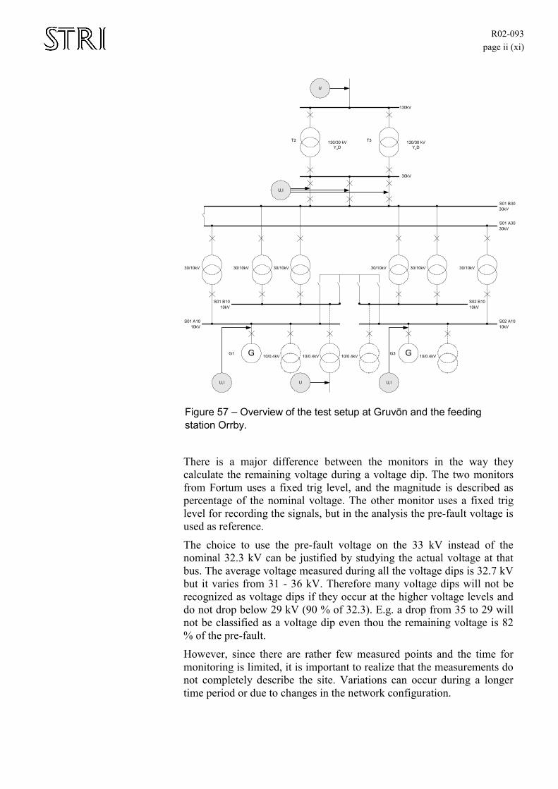
R02-093 page ii (xi)

G

130/30 kVYnD

130/30 kVYnD

T2 T3

30kV

G

S01 B30

S01 A30

S02 A10S01 A10

S01 B10 S02 B10

G3G1

U

U,I

U,I U,IU

30/10kV30/10kV 30/10kV 30/10kV 30/10kV 30/10kV

10/0.4kV10/0.4kV10/0.4kV 10/0.4kV

130kV

10kV

10kV

30kV

30kV

10kV

10kV

Figure 57 – Overview of the test setup at Gruvön and the feeding station Orrby.

There is a major difference between the monitors in the way they calculate the remaining voltage during a voltage dip. The two monitors from Fortum uses a fixed trig level, and the magnitude is described as percentage of the nominal voltage. The other monitor uses a fixed trig level for recording the signals, but in the analysis the pre-fault voltage is used as reference.

The choice to use the pre-fault voltage on the 33 kV instead of the nominal 32.3 kV can be justified by studying the actual voltage at that bus. The average voltage measured during all the voltage dips is 32.7 kV but it varies from 31 - 36 kV. Therefore many voltage dips will not be recognized as voltage dips if they occur at the higher voltage levels and do not drop below 29 kV (90 % of 32.3). E.g. a drop from 35 to 29 will not be classified as a voltage dip even thou the remaining voltage is 82 % of the pre-fault.

However, since there are rather few measured points and the time for monitoring is limited, it is important to realize that the measurements do not completely describe the site. Variations can occur during a longer time period or due to changes in the network configuration.

R02-093 page iii (xi)

Analysis of data The measured data was provided in data files and analysed. To get an overview of the voltage dip data, and to see how voltage dips propagated through the different voltage levels, a table with magnitude and duration for each phase at each voltage level was made. Many voltage dips have not been recorded simultaneously on all three monitors (the 130 kV monitor was out of order for two shorter periods).

Different analysis e.g. SARFI index, contour plots, ESKOM voltage dip index can be made with the data.

A more thorough study has been made on the data from the 30 kV busbar, since sampled signals were available. Every voltage dip has been analysed separately and the RMS-voltages, phase-angles between the phases and the symmetrical components have been calculated.

Representation of analysed data There are two major purposes with the representation and the analysis. The first one focus on to fully characterise and describe the voltage dips. The second purpose is to find methods present an overview of all voltage dips at the site.

4.7.5 SARFI index The purposes with the SARFI index is to compare the voltage dips at different voltage levels to each other and to compare voltage dip data with other sites.

A SARFI index has been calculated for each voltage level by using the nonzero measured points of each voltage level. The lowest phase voltage and the longest duration for each measured point were used for the index. The SARFI index is calculated for 90%, 85%, 80%, 70% and 60% remaining voltage. The result is shown in Figure 58.

The monitors at the different voltage levels have recorded a different number of voltage dips, and therefore a comparison between the voltage levels shall consider this. The number of recordings used in the voltage dip index for the 130 kV, 33 kV and the 400 V were 24, 22 and 46 respectively.

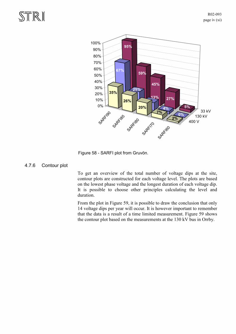
R02-093 page iv (xi)

SARFI90

SARFI85

SARFI80

SARFI70

SARFI60

400 V130 kV

33 kV

95%

59%

45%

27%

5%

67%

25%

13%

4%0%

35%

26%20%

7%2%

0%10%20%30%40%50%60%70%80%90%

100%

Figure 58 - SARFI plot from Gruvön.

4.7.6 Contour plot To get an overview of the total number of voltage dips at the site, contour plots are constructed for each voltage level. The plots are based on the lowest phase voltage and the longest duration of each voltage dip. It is possible to choose other principles calculating the level and duration.

From the plot in Figure 59, it is possible to draw the conclusion that only 14 voltage dips per year will occur. It is however important to remember that the data is a result of a time limited measurement. Figure 59 shows the contour plot based on the measurements at the 130 kV bus in Orrby.

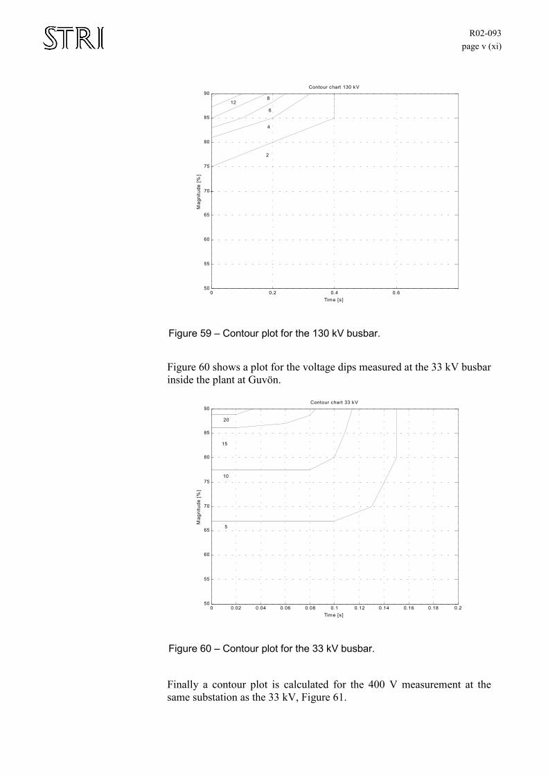
R02-093 page v (xi)

0 0.2 0.4 0.650

55

60

65

70

75

80

85

90

2

4

6

812

Contour chart 130 kV

Time [s]

Mag

nitu

de [

%]

Figure 59 – Contour plot for the 130 kV busbar.

Figure 60 shows a plot for the voltage dips measured at the 33 kV busbar inside the plant at Guvön.

0 0.02 0.04 0.06 0.08 0.1 0.12 0.14 0.16 0.18 0.250

55

60

65

70

75

80

85

90

5

10

15

20

Contour chart 33 kV

Time [s]

Mag

nitu

de [

%]

Figure 60 – Contour plot for the 33 kV busbar.

Finally a contour plot is calculated for the 400 V measurement at the same substation as the 33 kV, Figure 61.

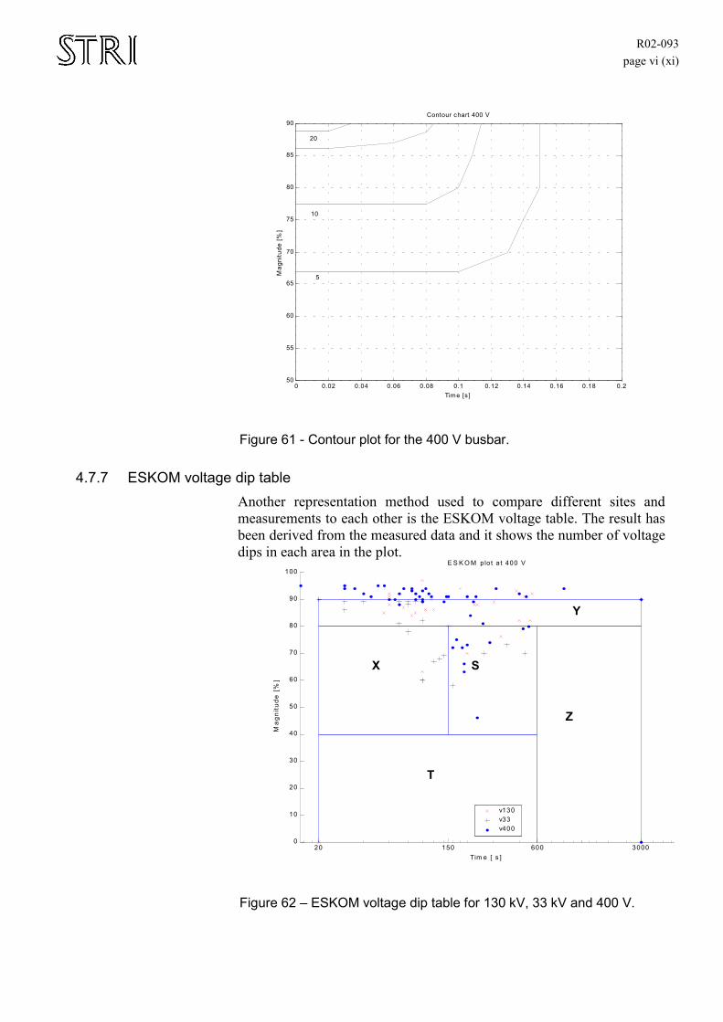
R02-093 page vi (xi)

0 0.02 0.04 0.06 0.08 0.1 0.12 0.14 0.16 0.18 0.250

55

60

65

70

75

80

85

90

5

10

20

Contour chart 400 V

Time [s]

Mag

nitu

de [

%]

Figure 61 - Contour plot for the 400 V busbar.

4.7.7 ESKOM voltage dip table Another representation method used to compare different sites and measurements to each other is the ESKOM voltage table. The result has been derived from the measured data and it shows the number of voltage dips in each area in the plot.

20 150 600 30000

10

20

30

40

50

60

70

80

90

100E S K O M plot a t 400 V

Tim e [ s ]

Ma

gnitu

de [

%]

v130v33v400

Figure 62 – ESKOM voltage dip table for 130 kV, 33 kV and 400 V.

T

X S

Z

Y

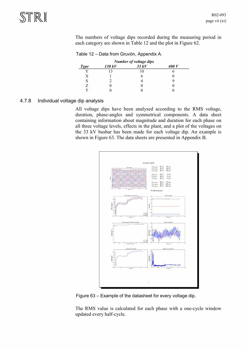
R02-093 page vii (xi)

The numbers of voltage dips recorded during the measuring period in each category are shown in Table 12 and the plot in Figure 62.

Table 12 – Data from Gruvön, Appendix A. Number of voltage dips

Type 130 kV 33 kV 400 V Y 13 10 6 X 1 6 0 S 2 4 9 Z 0 0 0 T 0 0 0

4.7.8 Individual voltage dip analysis All voltage dips have been analysed according to the RMS voltage, duration, phase-angles and symmetrical components. A data sheet containing information about magnitude and duration for each phase on all three voltage levels, effects in the plant, and a plot of the voltages on the 33 kV busbar has been made for each voltage dip. An example is shown in Figure 63. The data sheets are presented in Appendix B.

Figure 63 – Example of the datasheet for every voltage dip.

The RMS value is calculated for each phase with a one-cycle window updated every half-cycle.

R02-093 page viii (xi)

The phase angle between the three phases is calculated for every cycle.

The symmetrical components are calculated for every sample by first performing a FFT on the first cycle of the signal and then using the result to transform the three phases into the synchronous dq coordinate system. The signals are then transformed to positive-, negative- and zero-sequence voltages.

4.7.9 Dip propagation Studying the measured data and knowing the configuration of the system makes it possible to predict the propagation between the different voltage levels. A voltage dip can change type depending on the transformer it propagates through.

Yn yn 130/33 kV

Ynyn 33/10 kV

Dyn 10/0.4 kV

Figure 64 – Connection between the different voltage levels at Gruvön.

Table 13 – How different voltage dip types will propagate through the voltage levels, [28].

130 kV Ynyn 30 kV Ynyn 10 kV Dyn 400 V

A A A A B B B C

C C C D

E E E F

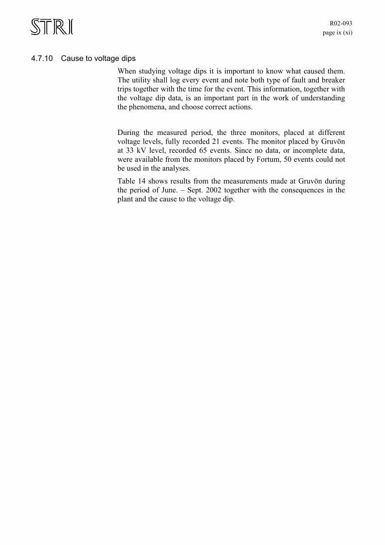
R02-093 page ix (xi)

4.7.10 Cause to voltage dips When studying voltage dips it is important to know what caused them. The utility shall log every event and note both type of fault and breaker trips together with the time for the event. This information, together with the voltage dip data, is an important part in the work of understanding the phenomena, and choose correct actions.

During the measured period, the three monitors, placed at different voltage levels, fully recorded 21 events. The monitor placed by Gruvön at 33 kV level, recorded 65 events. Since no data, or incomplete data, were available from the monitors placed by Fortum, 50 events could not be used in the analyses.

Table 14 shows results from the measurements made at Gruvön during the period of June. – Sept. 2002 together with the consequences in the plant and the cause to the voltage dip.

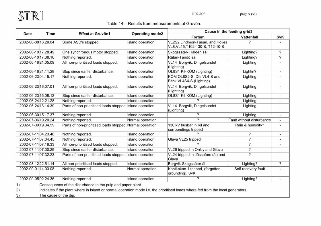
R02-093 page x (xi)

Table 14 – Results from measurements at Gruvön.

Cause in the feeding grid3 Date Time Effect at Gruvön1 Operating mode2 Fortum Vattenfall SvK

2002-06-08 16.29.04 Some ASD's stopped. Island operation VL2S2 Lindmon-Tåsan, and Höljes VL8,VL15,T102-130-S, T12-10-S

? -

2002-06-10 17.28.49 One synchronous motor stopped. Island operation Skogssäter- Halden såi Lighting? ? 2002-06-10 17.38.10 Nothing reported. Island operation Rätan-Tandö såi Lighting? ? 2002-06-18 21.05.09 All non-prioritised loads stopped. Island operation VL14 Borgvik, Dingelsundet

(Lighting) Lighting -

2002-06-18 21.11.28 Stop since earlier disturbance. Island operation OL8S1 Kil-KÖM (Lighting) Lightin? - 2002-06-23 04.15.17 Nothing reported. Island operation KÖM OL8S2-S, Dfs VL4-S and

Bäck VL4S4-S (Lighting) Lighting -

2002-06-23 16.07.01 All non-prioritised loads stopped. Island operation VL14 Borgvik, Dingelsundet (Lighting)

Lighting -

2002-06-23 16.08.12 Stop since earlier disturbance. Island operation OL8S1 Kil-KÖM (Lighting) Lighting - 2002-06-24 12.21.28 Nothing reported. Island operation ? Lighting - 2002-06-24 13.14.39 Parts of non-prioritised loads stopped. Island operation VL14 Borgvik, Dingelsundet

(Lighting) Lighting -

2002-06-30 15.17.37 Nothing reported. Island operation ? Lighting - 2002-07-06 19.20.24 Nothing reported. Normal operation ? Fault without disturbance - 2002-07-09 19.34.59 Parts of non-prioritised loads stopped. Normal operation 130 kV busbar in Kil and

surroundings tripped Rain & humidity? -

2002-07-11 04.23.48 Nothing reported. Island operation ? ? - 2002-07-11 07.04.45 Nothing reported. Island operation Glava VL25 tripped ? - 2002-07-11 07.18.33 All non-prioritised loads stopped. Island operation ? ? - 2002-07-11 07.30.29 Stop since earlier disturbance. Island operation VL26 tripped in Orrby and Glava ? - 2002-07-11 07.32.23 Parts of non-prioritised loads stopped. Island operation VL24 tripped in Jössefors (åi) and

Glava ? -

2002-08-12 22.51.14 All non-prioritised loads stopped. Island operation Borgvik-Skogssäter åi Lighting? ? 2002-09-01 14.03.08 Nothing reported. Normal operation Konti-skan 1 tripped, (forgotten

grounding), SvK Self recovery fault -

2002-09-05 02.24.36 Nothing reported. Island operation ? Lighting? - 1) Consequence of the disturbance to the pulp and paper plant. 2) Indicates if the plant where in Island or normal operation mode i.e. the prioritised loads where fed from the local generators. 3) The cause of the dip.

R02-093 page xi (xi)

Conclusions from the measurements and results It is important to use the same reference voltage, pre-fault or nominal, to compare the measured data from different voltage levels. It is preferable to use instruments that save sampled instantaneous values of the voltage dip, making different analyses possible. The time setting of the instruments must be coordinated, so that each event gets the same time stamp on all voltage levels. The trig level on each instrument shall result in a trig at all instruments for every voltage dip. One alternative is to have the instruments trig each other via an external signal. If one instrument is trigged, the other will also capture data.

Because of the malfunction of the monitor at the 130 kV busbar, data may be missing and therefore a comparison between the different voltage levels shall carefully be done. The utility companies Vattenfall and Fortum have provided the information of the dip causes.

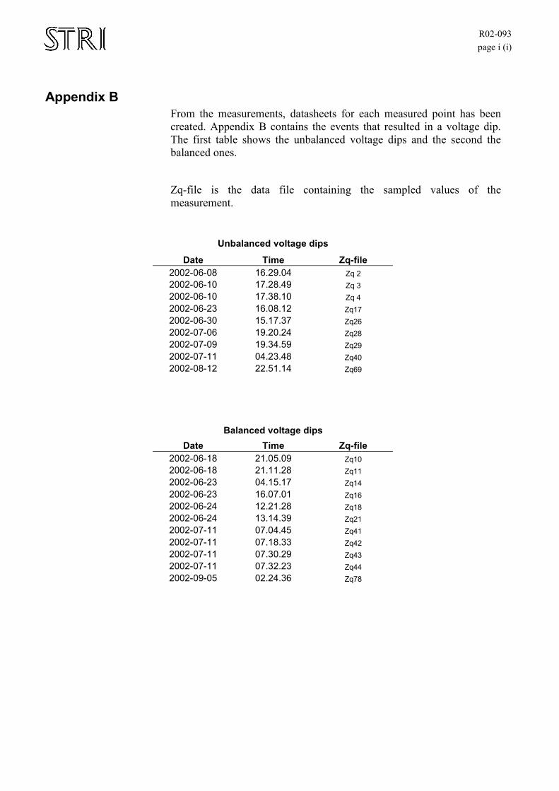
R02-093 page i (i)

Appendix B From the measurements, datasheets for each measured point has been created. Appendix B contains the events that resulted in a voltage dip. The first table shows the unbalanced voltage dips and the second the balanced ones.

Zq-file is the data file containing the sampled values of the measurement.

Unbalanced voltage dips Date Time Zq-file

2002-06-08 16.29.04 Zq 2 2002-06-10 17.28.49 Zq 3 2002-06-10 17.38.10 Zq 4 2002-06-23 16.08.12 Zq17 2002-06-30 15.17.37 Zq26 2002-07-06 19.20.24 Zq28 2002-07-09 19.34.59 Zq29 2002-07-11 04.23.48 Zq40 2002-08-12 22.51.14 Zq69

Balanced voltage dips

Date Time Zq-file 2002-06-18 21.05.09 Zq10 2002-06-18 21.11.28 Zq11 2002-06-23 04.15.17 Zq14 2002-06-23 16.07.01 Zq16 2002-06-24 12.21.28 Zq18 2002-06-24 13.14.39 Zq21 2002-07-11 07.04.45 Zq41 2002-07-11 07.18.33 Zq42 2002-07-11 07.30.29 Zq43 2002-07-11 07.32.23 Zq44 2002-09-05 02.24.36 Zq78

R02-093 page i (iii)

List of figures

Figure 1 – Illustration of a voltage dip with changing magnitude........................................................................................1 Figure 2 – A balanced 3-phase voltage dip. .........................................................................................................................4 Figure 3 – An unbalanced 3-phase voltage dip. ...................................................................................................................4 Figure 4 – Model for a balanced three-phase fault...............................................................................................................6 Figure 5 – Four types of voltage dips due to one- or three-phase fault. ...............................................................................7 Figure 6 – Three types of voltage dips due to two-phase fault.............................................................................................8 Figure 7 - Voltage dip related cost in different industries..................................................................................................13 Figure 8 – A normal single phase rectifier. ........................................................................................................................14 Figure 9 – An AC adjustable speed drive. .........................................................................................................................15 Figure 10 – Six-pulse rectifier............................................................................................................................................15 Figure 11 – Reference and saw tooth signal to obtain control signals. ..............................................................................16 Figure 12 – Control signals to the switches. ......................................................................................................................17 Figure 13 – Equivalent scheme for the DC-machine. ........................................................................................................17 Figure 14 – A typical industrial DC drive configuration. ..................................................................................................18 Figure 15 – Active power in a synchronous motor as a function of the load angle for different voltages. .......................23 Figure 16 – Immunity curve for semiconductor manufacturering equipment according to SEMI F47. ............................32 Figure 17 – Revised CBEMA curve, ITIC curve, 1996 [37]. ............................................................................................33 Figure 18 - Recommended layout for monitoring in a plant. .............................................................................................37 Figure 19 – Voltage-duration plot from Gruvön ................................................................................................................40 Figure 20 – Contour chart from Gruvön, Appendix A.......................................................................................................41 Figure 21 – SARFI plot for different busbars at Gruvön, Appendix A. .............................................................................42 Figure 22 – ESKOM voltage dip table...............................................................................................................................44 Figure 23 – Three-phase-voltages versus time for a voltage dip caused by a two-phase-fault (left) and a balanced three-

phase fault (right). ......................................................................................................................................................46 Figure 24 – RMS-voltage (left) and angle representation (right) for an unbalanced three-phase-voltage dip. ..................46 Figure 25 – A voltage dip caused by a two-phase fault (left) and the resulting symmetrical components (right). ............47 Figure 26 – Undelivered energy during a voltage dip as a function of magnitude and duration........................................47 Figure 27 – Example of representation of the number of voltage dips in each phase-angle-jump interval........................48 Figure 28 – The negative (left) and zero sequence component (right) for voltage dip Zq29, Appendix B........................49 Figure 29 - The procedure of the work using the method for evaluation of an industrial process according to voltage dips.

...................................................................................................................................................................................51 Figure 30 – Example of a process box representing a paper-machine in a pulp and paper mill. .......................................52 Figure 31 - An example of a plant described with three processes and a number of sub-processes. .................................53 Figure 32 - Different choices of the cost index. .................................................................................................................54 Figure 33 - Process 'A' with fault index 10 and cost index 30.000. ...................................................................................55 Figure 34 – Example of a plant interlocking chart. ............................................................................................................56 Figure 35 – An example of a process (paper machine) that has been divided into three sub-processes; A – Drying

section, B – Press section, C - Wire section. ..............................................................................................................58 Figure 36 - A process consisting of four sub-processes. ....................................................................................................59 Figure 37 – Examples of different rectangular magnitude variations during test and a real voltage dip. ..........................62 Figure 38 - Configuration for voltage dip immunity measurement....................................................................................63 Figure 39 – Contour chart combined with voltage tolerance curve for equipment I and II. ..............................................66 Figure 40 – ‘Complete’ model ...........................................................................................................................................67 Figure 41 – Improved immunity for sub-process ‘A.1’. ....................................................................................................68 Figure 42 – Removed interconnection between sub-process A.1 and A.2..........................................................................69 Figure 43 – Mitigation cost and responsibilities at different locations. .............................................................................75 Figure 44 – A radial network protected with fuses. ...........................................................................................................76 Figure 45 – Meshed network protected with distance protection.......................................................................................76 Figure 46 – Example of a site configuration with local generation and a 2-section busbar system. ..................................79 Figure 47 – An example of a configuration with two feeders and a HSSTS for switching the prioritised loads. ..............79 Figure 48 – A conventional motor-generator set................................................................................................................80 Figure 49 – A motor-generator set only using a synchronous machine. ............................................................................81 Figure 50 – Example of a standard UPS ............................................................................................................................81 Figure 51– Example of an off-line UPS.............................................................................................................................82 Figure 52 – Example of a standard configuration for a DVR. ...........................................................................................83

R02-093 page ii (iii)

Figure 53 – Example of the impact of an DVR installation to the immunity curve of a process. ..................................... 83 Figure 54– Example of a standard configuration for a shunt voltage controller. .............................................................. 84 Figure 55 – Combination of a DVR and SVC without energy storage.............................................................................. 84 Figure 56 – An example of an ride-through curve for a coil lock device [34]. ................................................................. 85 Figure 57 – Overview of the test setup at Gruvön and the feeding station Orrby. .............................................................. ii Figure 58 - SARFI plot from Gruvön. ................................................................................................................................ iv Figure 59 – Contour plot for the 130 kV busbar. .................................................................................................................v Figure 60 – Contour plot for the 33 kV busbar. ...................................................................................................................v Figure 61 - Contour plot for the 400 V busbar. .................................................................................................................. vi Figure 62 – ESKOM voltage dip table for 130 kV, 33 kV and 400 V. .............................................................................. vi Figure 63 – Example of the datasheet for every voltage dip. ............................................................................................ vii Figure 64 – Connection between the different voltage levels at Gruvön.......................................................................... viii

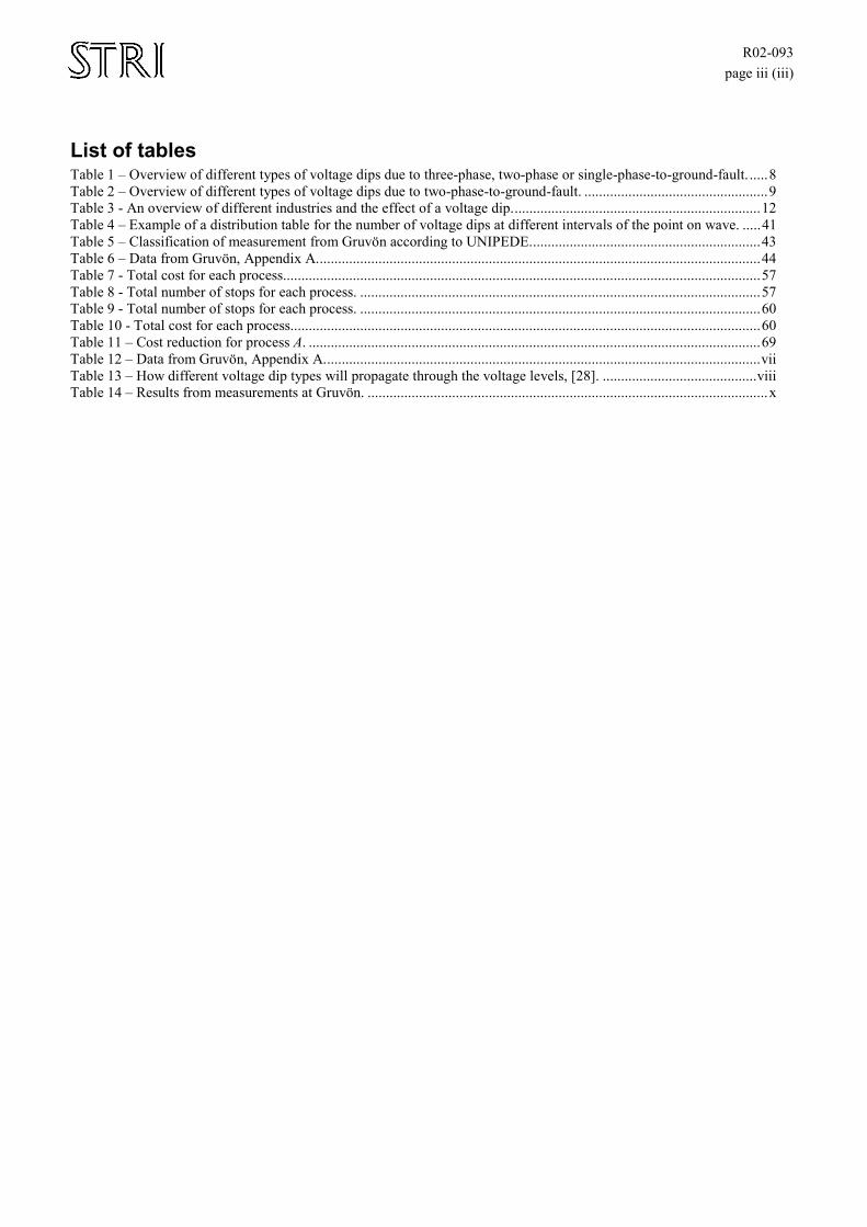
R02-093 page iii (iii)

List of tables Table 1 – Overview of different types of voltage dips due to three-phase, two-phase or single-phase-to-ground-fault. .....8 Table 2 – Overview of different types of voltage dips due to two-phase-to-ground-fault. ..................................................9 Table 3 - An overview of different industries and the effect of a voltage dip....................................................................12 Table 4 – Example of a distribution table for the number of voltage dips at different intervals of the point on wave. .....41 Table 5 – Classification of measurement from Gruvön according to UNIPEDE...............................................................43 Table 6 – Data from Gruvön, Appendix A.........................................................................................................................44 Table 7 - Total cost for each process..................................................................................................................................57 Table 8 - Total number of stops for each process. .............................................................................................................57 Table 9 - Total number of stops for each process. .............................................................................................................60 Table 10 - Total cost for each process................................................................................................................................60 Table 11 – Cost reduction for process A. ...........................................................................................................................69 Table 12 – Data from Gruvön, Appendix A.......................................................................................................................vii Table 13 – How different voltage dip types will propagate through the voltage levels, [28]. ..........................................viii Table 14 – Results from measurements at Gruvön. .............................................................................................................x