Universita degli Studi di Napoli Federico II

Facolta di Ingegneria

Corso di Studi in Ingegneria Informatica

TESI DI LAUREAin Ingegneria Informatica

Analysis of Prediction Techniques ofKey Parameters in IP Networks

Relatore

prof. Antonio Pescape

Candidato

Salvatore Giuliano

matr. 534/2961

Anno Accademico 2010-2011

dedica

Contents

1 Introduction 1

2 Introduzione 1

3 Analyzed Techniques : a Brief Review 33.1 Background on Time-Series . . . . . . . . . . . . . . . . . 3

3.1.1 Time-Series . . . . . . . . . . . . . . . . . . . . . . . 33.1.2 Time-Series Analysis . . . . . . . . . . . . . . . . . 43.1.3 Time-Series: A Glossary . . . . . . . . . . . . . . . 6

3.2 Model Based Prediction Methods . . . . . . . . . . . . . 83.2.1 Overview . . . . . . . . . . . . . . . . . . . . . . . . . 83.2.2 Autoregressive (AR) and Moving Average (MA)

Schemes . . . . . . . . . . . . . . . . . . . . . . . . . 83.2.3 Time-Series Decomposition Methods . . . . . . . 93.2.4 ARIMA models . . . . . . . . . . . . . . . . . . . . 103.2.5 FARIMA models . . . . . . . . . . . . . . . . . . . . 113.2.6 ARCH Models . . . . . . . . . . . . . . . . . . . . . 123.2.7 Exponential Smoothing Methods . . . . . . . . . . 123.2.8 Holt-Winters Forecasting Model . . . . . . . . . . 13

3.3 Learning Based Method : Artificial Neural Networks . 143.3.1 Computational Models of Neurons . . . . . . . . . 153.3.2 Artificial Neural Networks : A Taxonomy . . . . 163.3.3 The Learning Mechanism . . . . . . . . . . . . . . 173.3.4 Artificial Neural Network : Training . . . . . . . 183.3.5 (Focused)Time-Delay Neural Networks . . . . . . 193.3.6 Recurrent Neural Networks . . . . . . . . . . . . . 203.3.7 NARX Neural Networks . . . . . . . . . . . . . . . 21

4 Network Traffic Prediction : A Big Picture 254.1 Main Key Network Parameters Prediction . . . . . . . . 25

4.1.1 Throughput and Network Traffic Prediction . . . 25

i

CONTENTS ii

4.1.2 Predicting End-to-End Delay . . . . . . . . . . . . 274.1.3 Packet Loss Prediction . . . . . . . . . . . . . . . . 304.1.4 Available Bandwidth Forecast . . . . . . . . . . . 31

4.2 Network Technologies Across The Prediction Field . . 324.2.1 Related Works : a Taxonomy . . . . . . . . . . . . 33

4.3 Error and Performance Metrics . . . . . . . . . . . . . . . 35

5 Platforms and Toolkits 385.1 The MATrix LABoratory : MatLab . . . . . . . . . . . . 38

5.1.1 The MATLAB System . . . . . . . . . . . . . . . . 395.1.2 ToolBox . . . . . . . . . . . . . . . . . . . . . . . . . 405.1.3 System Identification Toolbox . . . . . . . . . . . . 415.1.4 Neural Network Toolbox . . . . . . . . . . . . . . 435.1.5 Predicting ”future” with NNToolbox . . . . . . . 44

5.2 The R-project . . . . . . . . . . . . . . . . . . . . . . . . . . 505.2.1 Time-Series representation and functions . . . . 525.2.2 Forecasting with R:A practical example . . . . . 54

6 Comparison of different techniques 566.1 Testbed . . . . . . . . . . . . . . . . . . . . . . . . . . . . . . 56

6.1.1 Data Sets . . . . . . . . . . . . . . . . . . . . . . . . 566.1.2 Techniques and Errors . . . . . . . . . . . . . . . . 606.1.3 Data set decomposition . . . . . . . . . . . . . . . . 61

6.2 Results and Errors Evaluation . . . . . . . . . . . . . . . 626.2.1 GPRS-to-wired traces . . . . . . . . . . . . . . . . . 626.2.2 MagNets Network . . . . . . . . . . . . . . . . . . . 686.2.3 SANET Network . . . . . . . . . . . . . . . . . . . . 78

6.3 Results and Evaluation tables . . . . . . . . . . . . . . . . 84

7 Conclusion and Future Works 102

List of Tables

3.1 ARIMA models key points . . . . . . . . . . . . . . . . . . . . . . . . . . . . . . . . . . . . 113.2 Holt-Winters models in key points . . . . . . . . . . . . . . . . . . . . . . . . . . . . . . . 153.3 Pros and Cons of Artificial Neural Networks . . . . . . . . . . . . . . . . . . . . . . . . . . 233.4 Classification of Techniques reviewed according to techniques previously explained. . . . . 24

4.1 Throughput Forecast Approaches . . . . . . . . . . . . . . . . . . . . . . . . . . . . . . . . 284.2 Traffic Forecast Approaches . . . . . . . . . . . . . . . . . . . . . . . . . . . . . . . . . . . 294.3 End-to-End Delay Forecast Approach . . . . . . . . . . . . . . . . . . . . . . . . . . . . . 304.4 Packet Loss Forecast Approaches . . . . . . . . . . . . . . . . . . . . . . . . . . . . . . . . 314.5 Network typologies . . . . . . . . . . . . . . . . . . . . . . . . . . . . . . . . . . . . . . . . 334.6 Hybrid models for Network Traffic Prediction . . . . . . . . . . . . . . . . . . . . . . . . . 354.7 Error Metrics in Prediction Fields . . . . . . . . . . . . . . . . . . . . . . . . . . . . . . . 37

5.1 Most used tools . . . . . . . . . . . . . . . . . . . . . . . . . . . . . . . . . . . . . . . . . . 385.2 Training Algorithms in Neural Network Toolbox software . . . . . . . . . . . . . . . . . . 475.3 Training stopping Criteria . . . . . . . . . . . . . . . . . . . . . . . . . . . . . . . . . . . . 48

6.1 SANET Data Traces: sampling and forecasts . . . . . . . . . . . . . . . . . . . . . . . . . 596.2 GPRS-to-wired trace MAEN Discussion . . . . . . . . . . . . . . . . . . . . . . . . . . . . 686.3 MagNet Short Term best MAEN overview . . . . . . . . . . . . . . . . . . . . . . . . . . . 786.4 SANET Link Load MAEN Discussion . . . . . . . . . . . . . . . . . . . . . . . . . . . . . 846.5 GPRS-to-wired-winlin TCP and UDP Error Results . . . . . . . . . . . . . . . . . . . . . 856.6 Results from gprs-to-wired-winlin TCP and UDP Error Evaluation . . . . . . . . . . . . . 866.7 MagNet Short Term Trace UDP Bitrate Error Results . . . . . . . . . . . . . . . . . . . . 876.8 Magnet Short Term UDP Delay Error Results . . . . . . . . . . . . . . . . . . . . . . . . . 886.9 Magnet Short Term UDP Jitter Error Results . . . . . . . . . . . . . . . . . . . . . . . . . 896.10 Magnet Short Term UDP PacketLoss Error Results . . . . . . . . . . . . . . . . . . . . . . 906.11 MagNet Short Term TCP Bitrate Error Results . . . . . . . . . . . . . . . . . . . . . . . . 916.12 MagNet Short Term TCP Delay Error Results . . . . . . . . . . . . . . . . . . . . . . . . 926.13 MagNet Short Term TCP Jitter Error Results . . . . . . . . . . . . . . . . . . . . . . . . . 936.14 MagNet Short Term Error Evaluation - Bitrate and Delay . . . . . . . . . . . . . . . . . . 946.15 MagNet Short Term Error Evaluation - Jitter and Packet Loss . . . . . . . . . . . . . . . 956.16 SANET Day Trace Error Result . . . . . . . . . . . . . . . . . . . . . . . . . . . . . . . . 966.17 SANET Week Trace Error Result . . . . . . . . . . . . . . . . . . . . . . . . . . . . . . . . 976.18 SANET Month Trace Error Result . . . . . . . . . . . . . . . . . . . . . . . . . . . . . . . 986.19 SANET Year Trace Error Result . . . . . . . . . . . . . . . . . . . . . . . . . . . . . . . . 996.20 SANET Error Evaluation Day and Week Trace . . . . . . . . . . . . . . . . . . . . . . . . 1006.21 SANET Error Evaluation Month and Year Trace . . . . . . . . . . . . . . . . . . . . . . . 101

iii

List of Figures

3.1 Example of artificial neuron with three inputs . . . . . . . . . . . . . . . . . . . . . . . . . 153.2 Multilayer perceptron architecture . . . . . . . . . . . . . . . . . . . . . . . . . . . . . . . 153.3 Different types of activation functions: (a) threshold, (b) piecewise linear, (c) Gaussian ,

and (d) sigmoid. . . . . . . . . . . . . . . . . . . . . . . . . . . . . . . . . . . . . . . . . . 163.4 Taxonomy of feedforward and feedback network architectures . . . . . . . . . . . . . . . . 173.5 Learning paradigms and algorithms . . . . . . . . . . . . . . . . . . . . . . . . . . . . . . . 183.6 A time-delay neural network. . . . . . . . . . . . . . . . . . . . . . . . . . . . . . . . . . . 203.7 NARX : Series-Parallel (SP) Mode . . . . . . . . . . . . . . . . . . . . . . . . . . . . . . . 223.8 NARX : Parallel (P) Mode . . . . . . . . . . . . . . . . . . . . . . . . . . . . . . . . . . . 22

5.1 Desktop Tools and Development Environment . . . . . . . . . . . . . . . . . . . . . . . . . 395.2 Ident GUI . . . . . . . . . . . . . . . . . . . . . . . . . . . . . . . . . . . . . . . . . . . . . 415.3 Simulation of AR System . . . . . . . . . . . . . . . . . . . . . . . . . . . . . . . . . . . . 435.4 GUI of Neural Network Toolbox . . . . . . . . . . . . . . . . . . . . . . . . . . . . . . . . 445.5 Matlab commands to create and visualize an FTDNN . . . . . . . . . . . . . . . . . . . . 455.6 Matlab commands to create and visualize a NARX . . . . . . . . . . . . . . . . . . . . . . 465.7 Training window . . . . . . . . . . . . . . . . . . . . . . . . . . . . . . . . . . . . . . . . . 495.8 Best Training Performance . . . . . . . . . . . . . . . . . . . . . . . . . . . . . . . . . . . 505.9 Time-series Response of a timedelaynet Training . . . . . . . . . . . . . . . . . . . . . . . 505.10 Best Validation Performance . . . . . . . . . . . . . . . . . . . . . . . . . . . . . . . . . . 515.11 Time-series Response of a narxnet Training . . . . . . . . . . . . . . . . . . . . . . . . . . 515.12 forecast() function . . . . . . . . . . . . . . . . . . . . . . . . . . . . . . . . . . . . . . . . 545.13 forecast() function with auto.arima() . . . . . . . . . . . . . . . . . . . . . . . . . . . . . 55

6.1 Gprs-to-wired-winlin-tcp dataset . . . . . . . . . . . . . . . . . . . . . . . . . . . . . . . . 586.2 Decomposition of a Time-Series using stl() function in R . . . . . . . . . . . . . . . . . . . 626.3 Prediction plots of Delay with ANN . . . . . . . . . . . . . . . . . . . . . . . . . . . . . . 646.4 Prediction plots of Delay with Holt-Winters and ARIMA . . . . . . . . . . . . . . . . . . 656.5 Prediction plots of Jitter with ANN . . . . . . . . . . . . . . . . . . . . . . . . . . . . . . 666.6 Prediction plots of Jitter with Holt-Winters and ARIMA . . . . . . . . . . . . . . . . . . . 676.7 Prediction plots of Bitrate with FTDNN and NARX . . . . . . . . . . . . . . . . . . . . . 696.8 Prediction plots of Bitrate with Holt-Winters and ARIMA . . . . . . . . . . . . . . . . . . 706.9 Prediction plots of Delay with FTDNN and NARX . . . . . . . . . . . . . . . . . . . . . . 716.10 Prediction plots of Delay with Holt-Winters and ARIMA . . . . . . . . . . . . . . . . . . 726.11 Prediction plots of Jitter with FTDNN and NARX . . . . . . . . . . . . . . . . . . . . . . 746.12 Prediction plots of Jitter with Holt-Winters and ARIMA . . . . . . . . . . . . . . . . . . . 756.13 Prediction plots of Packet Loss with FTDNN and NARX . . . . . . . . . . . . . . . . . . 766.14 Prediction plots of Packet Loss with Holt-Winters and ARIMA . . . . . . . . . . . . . . . 776.15 Link Load Prediction over a Gigabit Ethernet of COMP component of TRACE dataset

with TECH technique and H Horizon . . . . . . . . . . . . . . . . . . . . . . . . . . . . . 796.16 Link Load Prediction over a Gigabit Ethernet of COMP component of TRACE dataset

with TECH technique and H Horizon . . . . . . . . . . . . . . . . . . . . . . . . . . . . . 806.17 Link Load Prediction over a Gigabit Ethernet of COMP component of TRACE dataset

with TECH technique and H Horizon . . . . . . . . . . . . . . . . . . . . . . . . . . . . . 826.18 Link Load Prediction over a Gigabit Ethernet of COMP component of TRACE dataset

with TECH technique and H Horizon . . . . . . . . . . . . . . . . . . . . . . . . . . . . . 83

iv

Chapter 1

Introduction

”Why Prediction?”

This work would be a useful contribution to the students and researchersthat are interested in making a prediction and forecasting of IP networkparameters such as the Bitrate, Delay, Jitter, Packet loss and the Link Load.

Network performance prediction is an active area of research . In the lat-est studies, attention has been paid to the topic of complex networks, whichcharacterizes many natural and artificial systems such as airline transportsystems, power grid infrastructures, Internet and the World Wide Web.

For an Internet Service Provider the analysis of the network traffic throughthe links of its own network is needed for the critic operations regarding thenetwork’s resources.

For example, for an Internet Service Provider the analysis of the networktraffic through the links of its own network infrastructure is preparatoryto a set of critical operations relating to the management of the network’sresources.

To accurately and efficiently manage the resources of its infrastructure,the ISP must know the characteristics of traffic flows through it, in particular: bitrate, delay and Link Load. The knowledge of this last parameter enablesa basic capacity planning and resource provisioning activities.

A thorough knowledge of these parameters, thus, allow an optimization ofnetwork traffic flows, according to the quality requirements and the specificcharacteristics of the applications used by network users spread.

Various techniques of prediction are applied for this purpose. These tech-niques, starting from the time series of the interested network parameter,allow the network to obtain a projection of the behavior that the parameterwill take in future instants of time. An accurate prediction of various networkparameters reflect as accurately as possible the actual traffic patterns.

1

Prediction plays a fundamental role in the network’s performance im-provement. Several works which have been developed in the literature areinterested in resolving the problem of improving the efficiency and effective-ness of the network traffic. In fact there are many fields in which a predictionis made to monitor and improve systems and techniques.

A clear and reliable definition of prediction in this sense has not yet beenformulated. In general, a prediction or forecast is a statement about the waythings will happen in the future, often but not always based on experienceor knowledge. A prediction may be a statement with an expected outcome,while a forecast may cover a range of possible outcomes.

In order to provide a clear and reliable deal, a wide description of the mostwidely used techniques is proposed , platforms and tools in the predictionfield. All this stuff is supported by a massive comparison and analysis of themost used techniques over the various network technologies. A classificationof about an hundred of papers gives a big picture of the ”state of the art”and gives a point of view on future works and issues.

Next to this part, a chapter was completely dedicated to a description ofthe most used platforms and toolkits.

After this wide description of the state of the art, a description of theTestbed used for the implementation of the most effective techniques, inreference to some practical scenarios which foresee the analysis of Time seriesobtained by the WiFi MagNets network in Berlin, from configurations ofheterogeneous networks, and from the Slovak academic network SANET. Inparticular, for the first two cases, the data were extrapolated using the D-ITGsoftware developed by the Department of Computer and Systems Engineeringof the University of Naples ”Federico II”, while the SANET network datawere obtained using the software MRGT, Multi Router Traffic Grapher Tool.

At the end of this work there is a discussion about results and futurefollow-up.

2

Chapter 2

Introduzione

”Perche fare prediction?”

Questo lavoro vuole essere un utile contributo per studenti e ricercatoriche sono interessati nel fare prediction (predizione) e forecasting di parametricaratteristici di rete IP, tra cui il Bitrate, il Delay, il Jitter, il Packet lossed il Link Load. L’analisi e la prediction di tali parametri fornisce utiliinformazioni su quali sono i flussi critici e che quindi dovranno essere gestiticon particolare attenzione.

La previsione delle prestazioni di rete rappresenta un’attiva area di ricerca.In recenti studi molta attenzione e stata dedicata alla gestione ed ottimiz-zazione di reti complesse, che caratterizzano molti sistemi naturali e arti-ficiali, come sistemi di trasporto aereo, le infrastrutture di rete elettrica,Internet ed il World Wide Web.

Per un Internet Service Provider, ad esempio, l’analisi del traffico chetransita sui collegamenti (link) della propria rete e propedeutica ad un in-sieme di operazioni critiche relative alla gestione delle risorse della rete.

L’ISP per gestire in modo piu preciso ed efficiente le risorse della suainfrastruttura deve conoscere le caratteristiche dei flussi di traffico che la at-traversano, in particolare: il Bitrate, il Delay ed il Link Load. La conoscenzadi quest’ultimo parametro, abilita una basilare attivita di capacity planning(pianificazione della capacita) e resource provisioning (approvvigionamentodelle risorse).

Una conoscenza approfondita di questi parametri, quindi, permettera unaottimizzazione della gestione dei flussi di rete, tenendo anche conto dei req-uisiti di qualita e delle caratteristiche specifiche delle applicazioni utilizzatedagli utenti della rete stesa.

E a questo scopo che vengono applicate le varie tecniche di predictionche, partendo da serie storiche del parametro di rete interessato, consentono

1

di ottenere una proiezione del comportamento che il parametro assumera infuturi istanti di tempo. Un’accurata predizione dei vari parametri di reteriflette nel modo piu preciso possibile il reale andamento del traffico.

La previsione gioca quindi un ruolo fondamentale nel miglioramento delleprestazioni di una rete. Analizzando i parametri caratteristici di rete , qualiDelay , Packet Loss, Bitrate e Jitter e possibile capire aspetti importanti delflusso di dati che attraversa la rete e quindi agire per garantire una efficienzasempre maggiore.

Diversi documenti in letteratura sono volti a risolvere il problema dimigliorare l’efficienza e l’efficacia delle reti monitorandone e predicendoneil comportamento, tuttavia una definizione chiara e affidabile del termineprediction inteso in questo senso non e stata ancora formulata. In generale,fare ”prediction” o ”forecasting” consiste nel dare una dichiarazione sul modoin cui le cose accadranno in futuro (piu o meno prossimo), spesso ma nonsempre, sulla base di esperienza o conoscenza. La prediction puo essere in-tesa come una dichiarazione di qualcosa di aspettato, mentre il forecastingpuo coprire una vasta gamma di possibili risultati.

Al fine di fornire un documento chiaro e affidabile, e proposta un’ampiadescrizione delle tecniche piu diffuse. Le tecniche analizzate sono suddivisibiliin due gruppi distinti. Sono descritte tecniche basate su modelli e tecnichebasate su apprendimento. Una classificazione di circa un centinaio di docu-menti, completa il quadro generale dello ”stato dell’arte”. A seguire, un capi-tolo e stato interamente dedicato alla descrizione di alcune delle piattaformee dei toolkit piu utilizzati.

Dopo aver dato un’ampia descrizione dello stato dell’arte e descritto iltestbed utilizzato per l’implementazione delle tecniche piu affermate, in rifer-imento ad alcuni scenari pratici che vedono l’analisi di serie storiche ottenutedalla rete WiFi MagNets di Berlino, da configurazioni di rete eterogenee edalla rete accademica slovacca SANET. In particolare, per i primi due casi,i dati sono stati estrapolati utilizzando il software D-ITG sviluppato dal Di-partimento di Informatica e Sistemistica dell’Universita degli Studi di Napoli”Federico II”, mentre i dati relativi alla rete SANET, sono stati ottenuti uti-lizzando il software MRGT, Multi Router Traffic Grapher Tool.

A conclusione del presente lavoro vi e una discussione sui risultati rag-giunti e sui possibili follow-up relativi a questo lavoro.

2

Chapter 3

Analyzed Techniques : a BriefReview

Here it is a brief review of the most used techniques in prediction fields.After a background on Time-series, in this work, are presented two differentapproaches to perform traffic prediction. In first place are decrypted someof the most used techniques based on mathematical models (model-basedtechniques) and then is presented an approach based on learning (learning-based techniques).

3.1 Background on Time-Series

In this section a short but effective background on Time-Series (TS) is given.We refer to a survey on time series developed by Makridakis [127] and to thefundamental text on Time-Series realized by Jenkins [129]. After a formaldefinition of Time-Series and Time-Series Analysis, there is a glossary on TS[132] adapted to forecast problems, in order to have a quick reference of theterminology which is used.

3.1.1 Time-Series

A time series, z(t), is a set of observations ordered sequentially in time.Khintchine showed that it can be viewed as a sequence of the random vari-ables z1, z2, ..., zn, sampled at equidistant time intervals t1, t2, ..., tn. Eachtime point can be represented as:

zt = z′

t + ut (3.1)

where z′t is generated by the real process represented through the time se-

ries, and ut is a white noise term. Usually ut is expressed with a normal

3

distribution where:E[ut] = 0 (3.2)

and

E[utut+i] =

{σ2u if i = 0

0 if i 6= 0(3.3)

A key point is discovering some specifical characteristics of the time seriesin order to manipulate the data for several applications (in our case we referto forecasting).

3.1.2 Time-Series Analysis

Time-Series Analysis involves the analysis of data in order to discover theircharacteristics (stationarity, amplitude, frequency, phase). There are twomethods: Autocorrelation Analysis (AA) and Spectral Analysis (SA). TheAA uses autocorrelation function to analyze data in terms of their time char-acteristics (e.g. stationarity, seasonality). The SA uses the spectral functionto discover the frequency characteristics of the process (amplitude, frequency,phase). Moreover, AA enables us to determine if the series is stationary ornot, while SA allows us to estimate the gain function of a filter.

Stationarity

A time series is stationary if it has constant mean and variance. The mainadvantage of dealing with stationary series is that their statistical propertiesare independent from time and their stochastic characterization is easier.Since in practical problems a large number of actual time series are notstationary, there were developed several methods which allow us to transforma non-stationary series into one which is indeed stationary. A non-stationarytime series includes a trend element which can be represented by a functionof time:

Tt = a+ b1t+ b2t2 + b3t

3 + ... (3.4)

If we can estimate (3.37) and then subtract it (or divide it into) the timeseries zt, the result will be a de-trended series. In such a way we can applythe theory of stochastic process. Estimating Tt in (3.37) a problem mayoccur, due to the fact that we have to decide on the degree of polynomialto be fitted. Moreover, we have to decide how many terms (observations)we want to use in fitting the polynomial. To do this, we use an approachcalled ”method of moving average” by statisticians and ”low-pass filtering”by engineers.

4

Autocorrelation Analysis

Given the stationary time series (3.1):

zt = z′

t + ut

if we assume that ut is normally distributed, then zt can be described bymean, autocovariance and autocorrelation:

E[zt] =

n∑t=1

zt

n= z (3.5)

E[(zt − z)2] =

n∑t=1

(zt − z)2

n− 1= σ2 (3.6)

E[(zt − z)(zt+k − z)] =

n−k∑t=1

(zt − z)(zt+k − z)

n= γk (3.7)

E[(zt − z)(zt+k − z)]

E[(zt − z)2]=

n−k∑t=1

(zt − z)(zt+k − z)

n∑t=1

(zt − z)2

=γkσ2

= ρk (3.8)

If we accept the convention to substitute zt − z → zt, (3.7) and (3.8)become:

γk =

k∑t=1

ztzt+k

n(3.9)

ρk =

n−k∑t=1

ztzt+k

n∑t=1

z2t

(3.10)

Autocorrelations are measures of relationship between successive valuesof a variable ordered in time. They vary from −1 to +1 and, because of sta-tionarity, are even ρ−k = ρk. Autocorrelations are used for several purposes.For example they are used to determine the Existence of Stationarity. Theautocorrelation coefficients of a stationary time series go to zero quickly. Ifthis is not the case, the first difference should be taken and the autocorrela-tions of the de-trended series found. If they go to zero quickly, it means thatthe differenced series is stationary. And so on.

5

Spectral Analysis

If we consider the Fourier transform cosine of the autocorrelation functionwe obtain the Spectral Density Function S(f):

S(f) = 2

(1 + 2

n−1∑k=1

ρk cos 2πfk

)(3.11)

where the frequency f will always vary from 0 to 0.5, unless otherwisespecified.In a linear system in which Si(f) is the input spectra, So(f) the outputspectra and G(f) is the gain function between input and output, we havethat:

So(f) = Si(f) |G(f)|2 (3.12)

3.1.3 Time-Series: A Glossary

Time Series. A time series is a sequence of observations which are orderedin time (or space). The series value z is plotted on the vertical axis and timet on the horizontal axis. Time is called the independent variable. There aretwo kinds of time series data:

• Continuous, where we have an observation at every instant of time,e.g. electrocardiograms. We denote this using observation z at time t,z(t).

• Discrete, where we have an observation at (usually regularly) spacedintervals. We denote this as zt.

Trend. Trend is a long term movement in a time series. It is the underlyingdirection (an upward or downward tendency) and rate of change in a timeseries, when allowance has been made for the other components. A simpleway of detecting trend in seasonal data is to take averages over a certainperiod. If these averages change with time we can say that there is evidenceof a trend in the series. There are also more formal tests to enable detectionof trend in time series.

Seasonal Component. In daily, weekly or monthly data, the seasonal com-ponent, often referred to as seasonality, is the component of regular fluctu-ations in a time series which is dependent on a time period. For example,the costs of various types of fruits and vegetables, average daily rainfall and,in computer networks, network traffic intensity during different time of dayand night, all show marked seasonal variation.

6

Cyclical Component. In weekly or monthly data, the cyclical componentdescribes any regular fluctuations. It is a non-seasonal component whichvaries in a recognizable cycle.

Irregular Component. The irregular component is that left over when theother components of the series (trend, seasonal and cyclical) have been ac-counted for.

Smoothing. Smoothing techniques are used to reduce irregularities (randomfluctuations) in time series data. They provide a clearer view of the trueunderlying behavior of the series. In some time series, seasonal variation isso strong it obscures any trends or cycles which are very important for theunderstanding of the process being observed. Smoothing can remove season-ality and makes long term fluctuations in the series stand out more clearly.The most common type of smoothing technique is moving average smoothing.Since the type of seasonality will vary from series to series, so must the typeof smoothing.

Exponential Smoothing. Exponential smoothing is a smoothing techniqueused to reduce irregularities (random fluctuations) in time series data, thusproviding a clearer view of the true underlying behavior of the series. Italso provides an effective means of predicting future values of the time series(forecasting).

Moving Average Smoothing. A moving average is a form of averagewhich has been adjusted to allow for seasonal or cyclical components of a timeseries. Moving average smoothing is a smoothing technique used to make thelong term trends of a time series clearer. When a variable, like the numberof unemployed, or the cost of strawberries, is graphed against time, thereare likely to be considerable seasonal or cyclical components in the variation.These may make it difficult to see the underlying trend. These componentscan be eliminated by taking a suitable moving average. By reducing randomfluctuations, moving average smoothing makes long term trends clearer.

Differencing. Differencing is a popular and effective method of removingtrend from a time series. This provides a clearer view of the true underlyingbehavior of the series.

Autocorrelation. Autocorrelation is the correlation (relationship) betweensamples of a time series, such as the value of end-to-end delay or throughputand the same values at a fixed time interval later.

7

3.2 Model Based Prediction Methods

3.2.1 Overview

ARIMA model, also known as the Box-Jenkins methodology, is a gener-alized linear time-series analysis model and has been used to understandnetwork traffic. ARIMA/GARCH combines the linear ARIMA model withconditional variance GARCH (Generalized Auto Regressive Conditional Het-eroscedasticity). The differencing operator d in ARIMA can optionally befractional, giving rise to FARIMA models. The main drawback of theseapproaches is that they cannot predict far into the future because, by def-inition, they can only predict the patterns/trends they observe. Generally,time-series methods are used only in short term traffic prediction. For thissection we refer to [127], [129] for ARMA, ARIMA, FARIMA and Kalmanmodels, to [131] for Holt-Winters description and to [128] for ARCH modelsdescription.

3.2.2 Autoregressive (AR) and Moving Average (MA)Schemes

ARMA Schemes assume that a given value of time series is a weighted linearsum of past values and residual deviations. The following scheme (when v isequal to zero) is an autoregressive scheme.

zt+v =

p∑i=1

φtzt−i + εt+v (3.13)

= φ1zt−1 + φ2zt−2 + ...+ φpzt−p + εt+v

where φi represents the autoregressive parameters (or weights) and εt is theresidual deviation. Let us define a lag operator B as:

zt−1 = Bzt (3.14)

and let φ(B) be a polynomial in the operator B defined as follows:

φ(B) = (1− φ1B − ...− φpBp) (3.15)

Then the autoregressive process AR(p) can be represented as:

φ(B)zt = εt (3.16)

Since (3.16) implies:

zt =1

φ(B)εt = φ−1(B)εt (3.17)

8

the autoregressive process can be thought of as the output zt from a linearfilter with transfer function φ−1(B), when the input is εt. The following is amoving-average process

zt = εt −q∑

j=1

θjεt−j (3.18)

= εt − θ1εt−1 − θ2εt−2 − ...− θqεt−q

where εt and εt−j are the residual error at period t and t − j respectivelyand j is the moving-average parameter. We can also write the (3.18) in theequivalent form:

zt = (1− θ1B − θ2B2 − ...− θqBq)εt (3.19)

orzt = θ(B)εt (3.20)

Hence, the moving average process can be thought of as the output zt, froma linear filter with transfer function θ(B), when the input is εt.

The following is a mixed autoregressive/moving-average character

zt =

p∑i=1

φtzt−i + εt −q∑

i=1

θjεt−j (3.21)

= φ1zt−1 + φ2zt−2 + ...+ φpzt−p + εt − θ1εt−1 − θ2εt−2 − ...− θqεt−q

that is

(1− φ1B − φ2B2 − ...− φpB

p)zt = (1− θ1B − θ2B2 − ...− θqBq)εt (3.22)

orφ(B)zt = θ(B)εt (3.23)

where φi, θj and εt are defined as before and φ(B) and θ(B) are polynomials ofdegree p and q, in B. We subsequently refer to this process as an ARMA(p, q)process.

3.2.3 Time-Series Decomposition Methods

Time-Series Decomposition Methods work by either ”breaking up” the seriesinto trend, seasonal and remainder components, or by passing varying fre-quency filters through the data to separate low, medium or high frequencies.

9

3.2.4 ARIMA models

The Autoregressive Integrated Moving Average model of order (p, d, q), de-noted as ARIMA(p, d, q), is an extension to the ARMA(p, q) and it has theform:

zt =

p+d∑i=1

ϕizt−i +

q∑k=1

θkεt−k + εt (3.24)

where {ϕi}p+di=1 and {θk}qk=1 are respectively the autoregressive and moving

average parameters. Here, p stands for the autoregressive order, d for theorder of differencing, and q for the moving average order. The innovation(disturbance) variable εt is assumed to be an independent and identicallydistributed normal random variable with mean 0 and variance σ2. Thus,E[ε2

t |Ft−1] = σ2 where Ft−1 includes all the past information up to an in-cluding time t− 1, i.e., the innovation variance is time independent. As theprecedent assumptions, form (3.24) can be expressed as:

ϕ(B)∇dzt = θ(B)εt (3.25)

where ϕ(B) is a polynomial in B and ∇ is a difference operator, defined as:

(zt − zt−1) = ∇zt (3.26)

The ARIMA(p, d, q) is used to model homogeneous nonstationary time series.In order to build an ARIMA model, it is possible to use the Box-Jenkins

methodology, as follows:

1. Through transformations and/or differences variance is stabilized andthe series trend and stationarity are eliminated, then a stationary seriesis obtained.

2. For the obtained stationary series a model is identified and estimatedexplaining the structure of the time series correlation.

3. Model obtained in item 2 is applied inverse transformations allowingestablishing variability, trend, and stationarity for the original series.

4. Estimated model is validated through its residual correlation, whenthey show correlation it is necessary to estimate the parameters again,that is, to return to item 2. The previous iterative procedure is repeateduntil there is not any significant correlation between the residuals.

From an engineer’s point of view, differencing in ARIMA models act as high-pass filters on the trended data. The nonstationary behavior can be even

10

in terms of variance. The latter can become stationary by transforming thedata into a logarithmic scale or a fraction of a power (e.g. square root).

The latter can become stationary by transforming the data into a loga-rithmic scale or a fraction of a power (e.g., square root). In table 3.1 areexposed some key features of ARIMA models.

ARIMA models key points

Have three parts: the autoregression part (AR) that performslinear combination of previous observed values up to a definedmaximum lag (denoted p), the moving average part (MA) thattakes in count random error terms plus some linear combinationof previous random error terms up to a defined maximum lag (de-noted q), and the integration part (I) that takes in count the orderof differencing (denoted d) needed to reach the stationarity of thetime series. This means taking the differences between successiveobservations and then analysing these differences instead of theactual observations.Unlike ARMA models, can handle non-stationary time series;Can work only in the short and mean range of QoS forecastingperiods;Fitting ARIMA models to time series samples have a computa-tional complexity which is bounded by O(m3T ), where T is thelength of the time series sample, and m = max(p, q + 1);Cannot capture the bursty and non linear nature of the Inter-net traffic, due to the fact that ARIMA models have a constantvariance;Extreme outliers may bias the estimates of the seasonal and trendcomponents of ARIMA model;Estimation and validation is rather impractical for on-line fore-casting systems.

Table 3.1: ARIMA models key points

3.2.5 FARIMA models

The Fractional Autoregressive Integrated Moving Average process FARIMA(p, d, q)with 0 < d < 1/2 is a stationary process with long-range dependence. It isan extension to ARIMA(p, d, q) and defined as:

ϕ(B)∇dzt = θ(B)εt (3.27)

where the operator ∇d can be expressed using the binomial expansion:

∇d = (1−B)d =∞∑k=0

(d

k

)(−1)kBk (3.28)

FARIMA model are often used in prediction of long range dependent traffic.

11

3.2.6 ARCH Models

The ARIMA model with conditionally heteroskedastic disturbances can begiven by extending model (3.25) to allow the conditional variance of εt tochange over time. In addition to p + d + q parameters from the ARIMAmodel, conditionally heteroskedastic extension of order m introduces addi-tional m + 1 parameters. An ARIMA(p, d, q) − ARCH(m) (ARCH standsfor AutoRegressive Conditional Heteroskedasticity) model can be expressedas follows:

zt =

p+d∑i=1

ϕizt−i +

q∑k=1

θkεt−k + εt (3.29)

whereεt = ηt

√ht (3.30)

ht = α0 +m∑k=1

αkε2t−k (3.31)

where ηt is assumed to be an independent and identically distributed normalrandom variable with zero mean and unit variance. The additional m + 1parameters are {αi}mi=0. Note that disturbances εt are assumed to be uncorre-lated but not independent (higher moments may be correlated) unlike model(3.24), i.e., E[εtεt−1] = 0 and E[ε2

t ε2t−1] 6= 0. Under the given assumptions, it

follows then that the conditional distribution of εt, given the past informa-tion up to and including time t−1. This is normal with mean 0 and varianceht (time dependent).

3.2.7 Exponential Smoothing Methods

Exponential Smoothing Methods are special cases of autoregressive AR schemeswhen v < −1. Its weights φi in (3.13) decrease according to some exponentialfashion, thus the name ”exponential” is used. Exponential smoothing can beapplied to time series data, either to produce smoothed data for presenta-tion, or to make forecasts. When the sequence of observations begins at timet = 0, the simplest form of exponential smoothing is given by the formulas:

s1 = z0; (3.32)

st = αzt−1 + (1− α)st−1; (3.33)

where t > 1 and α is the smoothing factor, and 0 < α < 1. By directsubstitution of the defining equation for simple exponential smoothing back

12

into itself we find that:

st = αzt−1 + (1− α)st−1 (3.34)

= αzt−1 + α(1− α)zt−2 + (1− α)2st−2 (3.35)

= α[zt−1 + (1− α)zt−2 + (1− α)2zt−3 + (1− α)3zt−4 + ...] + (1− α)t−1z0

(3.36)

namely the weights assigned to previous observations are in general propor-tional to the terms of the geometric progression {1, (1 − α), (1 − α)2, (1 −α)3, ...}. A geometric progression is the discrete version of an exponentialfunction, so this is where the name for this smoothing method originated.The simple form (3.32) (3.33) of exponential smoothing is also known asan exponentially weighted moving average (EWMA). Technically it can alsobe classified as an Autoregressive integrated moving average ARIMA(0, 1, 1)model with no constant term.

3.2.8 Holt-Winters Forecasting Model

Holt-Winters methods are often used with seasonal time series. There aretwo kind of techniques: Additive Holt-Winters for additive seasonal charac-ters and Multiplicative Holt-Winters for multiplicative seasonal characters.Seasonality is additive if the seasonal effect increases with the level of thetime series. Seasonality is multiplicative if the seasonal effect is independentfrom the level of the time series. Holt-Winters model generalizes the expo-nential smoothing model. Let’s consider a phenomenon that has a lineartrend. It can be represented by a trend plus an irregular component:

zt = α + βt+ At t = 1, 2, ..., n (3.37)

Coefficients α and β can be found with the least squares method. We canuse the model in order to forecast the phenomenon a period forward:

zt+1|t = α + β(t+ 1) = α + βt+ β (3.38)

Generally:zt+l|t = α + β(t+ l) = α + βt+ lβ (3.39)

The trend at time t is Tt = α + βt while Ct = β is the level, that is theaverage level on which the series settles. Then

zt+l|t = Tt + lCt (3.40)

Parameters Tt and Ct can be written in a recursive form:

Tt = Tt−1 + Ct−1 (3.41)

13

Ct = Ct−1 (3.42)

with initial conditions T0 = α and C0 = β. Previous formulas can be gener-alized by Holt-Winters formulas:

zt+l|t = Tt + lCt (3.43)

where:Ct = αzt + (1− α)(Ct−1 + Tt−1) (3.44)

Tt = α(Ct − Ct−1) + (1− β)Tt−1. (3.45)

We can obtain α and β by minimizing the sum of the squares of forecasterrors:

S(α, β) =n∑

t=2

(zt − zt|t−1)2 t = 1, 2, ..., n (3.46)

Let consider a time series with a seasonal component St with period s.

zt+l|t = Ct + lTt + St+l−s l = 1, 2, ..., s (3.47)

Previous formulas are referred to additive seasonality (amplitude of seasonaleffects is constant in time series). When the effects of seasonality increasewith time, we’re in presence of the multiplicative seasonality. Formulas are:

Ct = αztSt−s

+ (1− α)(Ct−1 + Tt−1) (3.48)

Tt = β(Ct − Ct−1) + (1− γ)St−s (3.49)

and the prediction of l periods forward at time n is:

zt+l|t = (Ct + lTt)St+l−s l = 1, 2, ..., s (3.50)

In table 3.2 are shown some key points of Holt-Winters forecasting meth-ods.

3.3 Learning Based Method : Artificial Neu-

ral Networks

The ultimate goal of Artificial Neural Networks (ANNs) is to realize thelearning mechanisms of the human brain, making sure that the network in-teracts with the external environment without human intervention, as wellas that of creation. ANNs can be eyed as generalizations of mathematicalmodels of biological nervous systems. They are usually used to model com-plex i/o relationships or to find patterns in data. In [86] Hecht-Nielse providea formal definition of ANN .

14

Holt-Winters models key points

Often used with seasonal time series;The forecast is obtained as a weighted average of past observedvalues where the weights decline exponentially so that the valuesof recent observations contribute to the forecast more than thevalues of earlier observations;Two kinds of techniques: Additive Holt-Winters for additive sea-sonal characters and Multiplicative Holt-Winters for multiplica-tive seasonal characters;Simple exponential smoothing doesn’t have good performancewhen there is a trend in the data, Holt-Winters methods does;Holt-Winters techniques are sensitive to unusual events or outliers;

Table 3.2: Holt-Winters models in key points

DEFINITION: A neural network is a parallel, distributed informationprocessing structure consisting of processing elements (which can pos-sess a local memory and can carry out localized information processingoperations )interconnected together with unidirectional signal channelscalled connections. Each processing element has a single output con-nection which branches(”fans out”) into as many collateral connec-tions as desired (each carrying the same signal - the processing el-ement output signal). The processing element output signal can beof any mathematical type desired. All of the processing that goes onwithin each processing element must be completely local: i.e., it mustdepend only upon the current values of the input signals arriving at theprocessing element via impinging connections and upon values storedin the processing element’s local memory.

Figure 3.1: Example of artificial neuronwith three inputs Figure 3.2: Multilayer perceptron archi-

tecture

3.3.1 Computational Models of Neurons

Simple neuron (Figure 3.1) introduced by McCulloch and Pitts in 1940s [87],consists of input layer, activation function, and output layer. Input layer

15

receive input signal from external environment (or other neuron). Activationfunction is the neuron internal states that calculates and sum the inputsignals. The signals are then transmitted to output layer. The input layer,activation function and output layer in artificial neuron are similar to thefunction of dendrites, soma and axon in biological neuron.

The computational model of neurons is given from the following equation:

S = f

(n∑

j=1

wjxj

),

where xj is the actual input and wj the input weight. The function fis the transfer (or activation) function . The default transfer functions isthe sigmoid , but they may also take the form of other non-linear functions,piecewise linear functions or step functions( Figure 3.3 ). Generally, transferfunctions are monotonically increasing.

Figure 3.3: Different types of activation functions: (a) threshold, (b) piecewise linear, (c) Gaussian , and(d) sigmoid.

3.3.2 Artificial Neural Networks : A Taxonomy

Based on the connection pattern (architecture), ANNs can be grouped intotwo categories ([88] Jain and Mao, 1996) (Fig. 3.4):

• Feedforward networks, in which graphs have no loops

• Recurrent (or feedback) networks, in which loops occur because of feed-back connections.

In the most common family of feedforward networks, called multilayerperceptron(MLP), neurons are organized into layers that have unidirectionalconnections between them (Fig. 3.2).

16

Figure 3.4: Taxonomy of feedforward and feedback network architectures

3.3.3 The Learning Mechanism

The ability to learn is a fundamental trait of intelligence. Although a precisedefinition of learning is difficult to formulate, a learning process in the ANNcontext can be viewed as the problem of updating network architecture andconnection weights so that a network can efficiently perform a specific task.The network usually must learn the connection weights from available train-ing patterns. Performance is improved over time by iteratively updating theweights in the network.

A learning algorithm refers to a procedure in which learning rules areused for adjusting the weights.

There are two main learning paradigms: supervised and unsupervised.In supervised learning, or learning with a teacher, the network is providedwith a correct answer (output) for every input pattern. Weights are deter-mined to allow the network to produce answers as close as possible to theknown correct answers. Reinforcement learning is a variant of supervisedlearning in which the network is provided with only a critic on the correctnessof network outputs, not the correct answers themselves. In contrast, unsu-pervised learning, or learning without a teacher, does not require a correctanswer associated with each input pattern in the training data set. It ex-plores the underlying structure in the data, or correlations between patternsin the data and organizes patterns into categories from these correlations.

Each learning algorithm is designed for training a specific architecture.Therefore, when we discuss a learning algorithm, a particular network archi-tecture association is implied. Each algorithm can perform only a few tasks

17

well ([88]Jain and Mao, 1996) (Fig. 3.5).

Figure 3.5: Learning paradigms and algorithms

3.3.4 Artificial Neural Network : Training

Training the network is time consuming. It usually learns after severalepochs, depending on how large the network is. We could also stop thetraining after the network meets certain stopping criteria as minimum gra-dient magnitude, maximum training time , minimum performance value etc.

The best training procedure is to compile a wide range of examples whichexhibit all the different characteristics of the problem. To obtain a robustand reliable network it is needed to add some noise to the training data toget the network familiarized with noise and natural variability in real data.

18

How many neurons?

Selection of the number of hidden neurons is a crucial decision. The numberof hidden neurons affects how well the network is able to separate the data. Alarge number of hidden neurons will ensure correct learning, and the networkis able to correctly predict the data it has been trained on,but its performanceon new data, its ability to generalize, is compromised. With too few hiddenneurons, the network may be unable to learn the relationships amongst thedata and the error will fail to fall below an acceptable level. It is evident thatwe must find the right compromise during the selection of hidden neuronsnumber

About Initial Weights and Learning Rate

There are no recommended rules for the initial weights selection except tryingseveral different starting weight values to see if the network results are im-proved. The learning rate is a value that controls the size of the adjustmentsmade during the training process. If the learning rate is too high, then thealgorithm learns quickly but we have oscillations during the training process,if it is lower then the predictions jump around less, but the algorithm takesa lot longer to learn.

3.3.5 (Focused)Time-Delay Neural Networks

Time-Delay Neural Networks (TDNN) consist in a feedforward network witha tapped delay line at the input. It is similar to a multilayer perceptron inthat all connections feed forward (Figure 3.6). In the TDNN, the inputs toany node can consist of the outputs of earlier nodes during some numbers ofprevious time steps. This is generally implemented using tap-delay lines.

A natural restriction of the general TDNN topology is the class of TDNNarchitectures which have delays only on the input units known as FocusedTime-Delay Neural Network (FTDNN)[133].

Still in [133], the authors make a characterization and contrast the ca-pabilities of the general class of time-delay neural networks(TDNN’s) withinput delayed neural networks(FTDNN’s), the subclass of TDNN’s with de-lays limited to the inputs, that they call IDNN’s.

FTDNN can be viewed as the most straightforward dynamic networks.In Figure 3.6 is shown a time-delay neural network architecture that is

equivalent to a single hidden layer feedforward neural network. This networkmaps a finite time sequence (3.51) in a single output y that is given from theequation 3.52.

19

Figure 3.6: A time-delay neural network.

{x(t), x(t−∆), x(t− 2∆), .., x(t−m∆)} (3.51)

y =J∑

j=1

αjf

(m+1∑i=1

wjix(t− (i− 1)∆)

)(3.52)

where f is the activation of hidden units and ∆ is the Delay associatedto the input layer.

3.3.6 Recurrent Neural Networks

Recurrent Neural Networks(RNNs) are the state of the art in nonlineartime series prediction, system identification, and temporal pattern classifi-cation. Contrary to feedforward networks, recurrent neural networks can besensitive, and be adapted to past inputs. Recurrent neural networks are com-plex parametric dynamic systems that can exhibit a wide range of differentbehavior.

Simple recurrent networks (SRNs) comprise a class of recurrent neuralmodels that are essentially feedforward in the signal-flow structure, but also

20

contain a small number of local and/or global feedback loops in their archi-tectures. A state layer is updated not only with the external input of thenetwork but also with activation from the previous forward propagation. Thefeedback is modified by a set of weights as to enable automatic adaptationthrough learning.

Some popular recurrent network architectures are the Elman recurrentnetwork [89] in which the hidden unit activation values are fed back to anextra set of input units and the Jordan recurrent network in which outputvalues are fed back into hidden units.

3.3.7 NARX Neural Networks

The last mentioned recurrent architectures are usually trained by means oftemporal gradient-based variants of the backpropagation algorithm. How-ever, learning to perform tasks in which the temporal dependencies present inthe input/output signals span long time intervals can be quite difficult usinggradient-based learning algorithms. In [90], the authors report that learningsuch long-term temporal dependencies with gradient-descent techniques ismore effective in a class of SRN model called Nonlinear Autoregressivewith eXogenous input (NARX) [91] than in simple MLP-based recurrentmodels.

Despite the aforementioned advantages of the NARX network, its feasi-bility as a nonlinear tool for univariate time series modeling and predictionhas not been fully explored yet.Potential fields of application of our approach are communication networktraffic characterization [92][93] and chaotic time series prediction [94], sinceit has been shown that these kinds of data present long-range dependencedue to their self-similar nature.

This kind of network can be used as a tool for nonlinear system identifi-cation with excellent results. In [125] is proposed a way to solve efficientlythe issue of nonlinear time series prediction with the NARX network. Theypropose a simple strategy to allow the computational resources of the NARXnetwork to be fully explored in nonlinear time series prediction tasks.

The Nonlinear Autoregressive model with Exogenous inputs (NARX) [95]is an important class of discrete-time nonlinear systems that can be mathe-matically represented as :

21

y(n+1) = f [y(n), ..., y(n−dy +1); u(n), u(n−1), ..., u(n−du+1)]; (3.53)

where u(n) ∈ R and y(n) ∈ R denote, respectively, the input and outputof the model at discrete time step n , while du ≥ 1 and dy ≥ 1, du ≥ dy, arethe input-memory and output-memory orders.

that may be written as :

y(n+ 1) = f [y(n);u(n)]; (3.54)

where the vectors y(n) and u(n) denote the output and input regressors,respectively.

The nonlinear mapping f(·) is generally unknown and can be approxi-mated, for example, by a standard multilayer Perceptron (MLP) network.The resulting architecture is then called a NARX network [96][97].

NARX training

As we can see in [125], there are two configurations for the NARX networks:

• Series-Parallel (SP) Mode - In this case, the output’s regressor isformed only by actual values of the system’s output:

y(n+ 1) = f [ysp(n);u(n)], (3.55)

y(n+ 1) = f [y(n), ..., y(n− dy + 1);u(n), u(n− 1), ..., u(n− du + 1)];(3.56)

Figure 3.7: NARX : Series-Parallel (SP)Mode

Figure 3.8: NARX : Parallel (P) Mode

22

• Parallel (P) Mode - In this case, estimated outputs are fed back andincluded in the output’s regressor:

y(n+ 1) = f [yp(n);u(n)], (3.57)

y(n+ 1) = f [y(n), ..., y(n− dy + 1);u(n), u(n− 1), ..., u(n− du + 1)];(3.58)

In order to perform a good training the Series-Parallel configuration (openloop) is the right choice, while the Parallel configuration (closed loop) isuseful for testing and multi-step-ahead prediction. In table 3.3 there is ashort summary of ANN characteristics, while in table 3.4 there is a taxonomyreferred to all techniques reviewed in this work.

PRO CONS

Able to easily handle a greatamount of information

Can require considerable param-eter tweaking and retraining tofit well

Good behavior with noisy signals Training is time consumingAble to generalize the expertknowledge

Can suffer from ”interference” inthat new data can cause ANN toforget some of what it learned onold data

Can be trained directly on datawith thousands of inputs

Training is computationally ex-pansive

Fast prediction speed Hard to see how input variablesaffect the responses (BLACKBOX)

Table 3.3: Pros and Cons of Artificial Neural Networks

23

Tab

le3.4

:C

lass

ifica

tion

of

Tec

hn

iqu

esre

vie

wed

acc

ord

ing

tote

chn

iqu

esp

revio

usl

yex

pla

ined

.

Tec

hniq

ues

Ref

eren

ces

AR

(MA

)[6

7,49,

55,

72,

20,

71,

8,56,

1]A

RIM

A[3

1,36,

8,66,

54,

60,

12,

41,

21,

17,

53,

72,

62]

Hol

t-W

inte

rs[3

6,30,

70,

5,49

]N

eura

lN

etw

orks

[11,

52,

47,

43,

18,

6,33

,36

,70

,5,

46,

28,

8,66

,60

,58

,64

,10

][7

4,35

,34

,76

,15

,48

,65

,9]

Hybri

dM

odel

s[8,

27,

9,40

]

24

Chapter 4

Network Traffic Prediction : ABig Picture

4.1 Main Key Network Parameters Predic-

tion

4.1.1 Throughput and Network Traffic Prediction

Throughput can be defined as the average rate of a successful packet deliv-ery over a communication channel in a network. Spectral Efficiency refers tothe information rate that can be transmitted over a given bandwidth and is

measured inbit/s

Herz. Since in the first communication systems the spectral ef-

ficiency was equal to one, still today the terms bandwidth and throughput areoften used interchangeably. Obviously, when we’re talking about throughputprediction on an Internet network, we have to specify which transport proto-col we refer to, TCP or UDP. Throughput prediction has several applications:by improving this task, for example, network providers can optimize networkresources, offering the possibility to ensure a better quality of service. Also,traffic forecasting can help to detect anomalies as security attacks or virusesby comparing the real traffic with the forecasts, as explained in [23].From the several approaches to throughput prediction we can cite formula-based approaches and history-based approaches [49]. The first predicts through-put using mathematical expressions that involve, in the case of TCP trans-port protocol, sender’s behavior to path and end-host properties (RTT,packet loss rate, receive window size). All these data are plugged into aformula to generate the predicted values. The latter is generally more ac-curate and typically use some kind of standard time series forecasting based

25

on throughput measurements and derived from prior file transfers. One ofbiggest problems with network throughput prediction is that the probabilitydistribution of traffic is unclear and the scale and bandwidth of networks areconstantly changing. Moreover, network throughput is much more difficultto predict than end-to-end delay, since throughput has a strongly nonlinearbehavior (see [1]).The conception of throughput prediction is different from the concept oftraffic prediction. Essentially because, in the case of throughput, the rate atwhich packets are transmitted on the network is known. From time seriesmodeling point of view, Holt-Winters (See section 3.2.8) methods were devel-oped for series with trended and seasonal factors, model such as ARMA (seeSection 3.2.2), ARIMA (see Section 3.2.4)and Fractional-ARIMA (see Sec-tion 3.2.5) are not able to take in count the non-linear behavior of Internettraffic, though ARIMA can capture the nonstationary behavior of traffic .Moreover, network traffic is self similar in nature (self-similarity is the prop-erty of a series of data points to retain a pattern or appearance regardlessof the level of granularity used), showing high burstiness in a wide range oftime scales and obey in the heavy-tail distribution. In the case of TCP flows(TCP is the dominant transport protocol of the network such Internet), con-gestion window, presence of acknowledgements, multiplexing of packets atbottleneck rate contribute to the propagation of the self-similarity nature ofthe traffic. From this point of view all these models have a constant variance,and thus cannot capture the real bursty nature of the Internet traffic. Thisaspect can be solved using ARCH models (see Section 3.2.6) and its variantsor with Gegenbauer ARMA (GARMA) models, as written in [44]. Anothersolution can be using Artificial Neural Network (ANN) Approaches (see Sec-tion 3.3) that are capable of predicting self-similar traffic. Information likethroughput are used also for bandwidth provisioning, like in [19].Also SVR method demostrated some useful aspects in throughput predic-tion: it can accept multiple inputs (i.e., multivariate features) and will useall of these to generate the throughput prediction. Moreover SVR does notcommit to any particular parametric form, unlike formula-based approaches.Instead, SVR models are flexible based on their use of so-called nonlinearkernels. This expressive power is the reason why SVR has potential to bemore accurate than prior methods. Finally, SVR is computationally efficient,which makes it attractive for inclusion in a tool that can be deployed andused in a wide area.

Specifically, in [31] Anand et al. developed a non-linear time series model,expanding the concept of ARCH with GARCH model (Generalized AutoRe-gressive Conditional Heteroskedasticity), with innovation process general-ized to the class of heavy-tailed distributions. Results showed that GARCH

26

prediction performance are significantly better if compared with ARIMA,ARCH, ARIMA-ARCH models. In [21] ARIMA models are compared withANFIS models in WiMax network.

Another method examined in literature is SVR. In [67] Rossi et al.explorethe use of Support Vector Regression models for the purpose of link loadforecast, comparing the performance with Moving Average (MA) and Auto-Regressive (AR) models. Results showed that, despite a not powerful gainfor prediction at short time scales, SVR methods are still robust to parametervariations, are scalable and they lead to a significantly extend of the forecasthorizon. Another paper [13] compare CDF predictor performance with SVRpredictor one demonstrating that its prediction accuracy is higher. And in [3],Mirza et al. made SVR prediction and investigated the relationship betweenTCP throughput and measurements of path properties including availablebandwidth, queuing delays and packet loss.

From the point of view of neural networks, [33] focused the neural net-work based on multi-layer perceptron (MLP) and trained by Levenberg- Mar-quardt (LM) and the Resilient back propagation (Rp) algorithms, while in[64], [10] Li et al. focused on a network traffic forecasting strategy based onBP neural network (BP-NTF). In [36] Cortez et al proposed a comparativestudy between Holt-Winters, the ARIMA methodology and a Neural NetworkEnsemble (NNE) approach. In particular, the latter produces the lowest er-ror, in both realtime and short-term traffic analysis. Similar comparison wasmade by Feng et al. in [66], analyzing ARIMA, FARIMA (see also [72]), ANNand Wavelet predictors and comparing their performance with MSE, NMSE.Results showed significant advantages for the ANN technique. Even fromANN related studies, Junsong et al. in [60] compared the Elman Neural Net-work prediction performance with the one obtained with ARIMA, FARIMA,ANN and Wavelet predictors, obtaining significantly lower prediction errors(MSE and NMSE).

Other studies [46], [45], [69], proposed tools to forecast network traffic.In particular, Eswardass et al. in [46] proposed an improvement on Net-work Weather Service based on Artificial Neural Network, ensuring betterperformances in terms of accuracy.

In [59] Goya et al. proposed a method to derive analytic models thatpredict the throughput of TCP flows between two nodes using network char-acteristics such as loss and delay and modifying the Amherst model.

4.1.2 Predicting End-to-End Delay

The delay of a network it’s a measure of the time needed for a bit of datato travel across the network from one node to another. There are two kinds

27

Table 4.1: Throughput Forecast Approaches

Techniques and variants Section ReferencesAR(MA) Section 3.2.2 [20]

Neural Networks Section 3.3 [46],[3]

of delays: Hop-by-Hop delay and End-to-End delay. End-to-end delay is thesum of delays experienced at each hop, from the source to the destination.There are requirements on end-to-end delay for many Internet real-time ap-plications, such video-conferencing, VoIP, streaming applications and dis-tributed games. Moreover, delay-based approach is used to predict networkcongestion, to design network protocols and flow control algorithms and tomake analytical studies of network configurations. The end-to-end delay maybe considered as the sum of two principal components: a constant componentwhich includes the propagation delay and transmission delay and a variablecomponent which includes the processing and queuing delay. The last com-ponent is the major source of uncertainty. Parameters that are often used inthis field to understand the Internet dynamics are Round Trip Time (RTT),that needs measurements only at one end, and One-way Transmission Time(OTT), that requires the involvement of the receiver to obtain the measure.In [98] and [79] is shown that the mean OTT can’t be approximated withhalf RTT.For time series data that are stationary, it is possible to use ARMA model (seeSection 3.2.2) but most time series data of Internet end-to-end delay are non-stationary so other models like ARIMA models (see Section 3.2.4) are needed.For example [24] proposed a method based on Maximum Entropy Principle(MEP) instead of ARMA model, obtaining better performance, since some-times delays develop with quick variation. In another work Miloucheva etal. [12] combined ARIMA prediction and outlier detection for short-termand medium-term forecasting, using end-to-end delay QoS measured data.Results showed also that outliers could corrupt the forecasting values for thedelay. On the practical point of view, end-to-end delay of a TCP flow is anoisy, nonstationary and nonlinear process, but if the traffic intensity is low,we can observe a stationary behavior. This is very useful for long-horizonend-to-end delay forecasting. In fact, results from [40] showed that on long-horizon end-to-end delay forecasts, an hybrid approach based on discretewavelet transform, neural network and the k-nearest neighbors techniquesperforms better than [34] for longer forecasts an performs worse for shorterforecasts (around 64 steps ahead). Recently literature started to analyze thequestion of end-to-end delay forecasting jointly with other parameters like

28

Tab

le4.2

:T

raffi

cF

ore

cast

Ap

pro

ach

es

Tec

hniq

ues

and

vari

ants

Sec

tion

Ref

eren

ces

AR

(MA

)Sec

tion

3.2.

2[4

4],

[49]

,[67

]H

olt-

Win

ters

Sec

tion

3.2.

8[4

9],

[36]

,[70

]A

RIM

ASec

tion

3.2.

4[2

1],[36

],[4

1],[60

],[6

6],[72

]N

eura

lN

etw

orks

Sec

tion

3.3

[9],[1

0],[11

],[2

3],[30

],[3

3],

[36]

,[48

],[6

0],[65

],[6

6],[76

],[6

4]A

RC

HSec

tion

3.2.

6[1

9],[31

]

29

Table 4.3: End-to-End Delay Forecast Approach

Techniques Section ReferencesAR(MA) Section 3.2.2 [56],[54],[1],[20]ARIMA Section 3.2.4 [12]

Neural Networks Section 3.3 [40],[34],[43]

throughput, in order to use the possible statistical dependence with end-to-end delay. In fact, Mendoza et al. in [1] made a comparison betweenAR, SVM (individual version and joint version including information aboutthroughput) and Kalman techniques that showed SVMs models are the bestpredictor for individual or joint versions. Worse performances are with ARpredictor. Problems of delay boundary prediction were studied in [37], and[24].

AR,MA or ARMA [56],[54],[1],[20], ARIMA [12], SVM [1], Neural Net-works [40],[34],[43] and their variants, are used to forecast end-to-end delaytime series. Other studies [25],[32] involve Hidden Markov Model (HMM) inorder to model delay behavior. Multiple Model (MM) proposed in [55] uses aset of models that is assumed to describe the system dynamics through a bankof filters that runs in parallel at the same time and provides a non-stationaryand non linear solution for delay prediction. Experimental results shows thistechnique works better than Least Mean Square (LMS) and Recursive LeastSquare (RLS), two most widely used linear adaptive filters. Studies on theInternet delay dynamics [34] showed the success of dynamic neural networksas semi-parametric approximators for modeling complex systems involved inthis type of phenomena, but it remains an open problem applying neuralnetwork method to forecast delay online [43].

4.1.3 Packet Loss Prediction

Packet Loss prediction has gained much interest in last years for many rea-sons. Monitoring and forecasting packet loss behavior is very quick way totrack congestion conditions of a network. In fact, if congestion occurs on alink carrying TCP as well as UDP traffic, TCP will react by reducing thetraffic rate, while UDP will not. The rate adjustment is based on packet-lossrate and the round-trip time (RTT). Rather than using previously measuredvalues of packet loss and RTT (a causal effect of RTT on packet loss rate isalso demonstrated), a better approach is to use predictions of these quanti-ties. Such a predictive approach will be quicker to track congestion conditionsthan the typically used reactive approach. Moreover, increasing applications

30

Table 4.4: Packet Loss Forecast Approaches

Techniques and variants Section ReferencesNeural Networks Section 3.3 [51],[102],[103]Other methods [104],[101],[99],[100], [57]

in transmitting audio and video services over IP networks require mecha-nisms to prevent situation that can determine the degradation of video andaudio real time quality, as packet loss situations do. Studies on packet lossprediction are also useful in the wireless sensor networks, in indoor and out-door environment, since they offer the capability of determining the numberof motes, sampling rate and the operational environment to obtain a reliabledata transfer for a given sensing application. Packet loss is strongly influ-enced by Throughput (see [53]) and Long-range Dependent (LRD) NetworkTraffic. In fact, several studies showed the greater the LRD, the lower theQuality of Service. Nevertheless, in literature there are not so many workson Packet Loss Prediction. Su et al. [99] derived the packet loss probabil-ity, conditioned on past loss rates, assuming the Gilbert model, which is asimple two-state Markov model. Salvo Rossi et al. [100] modeled end-to-endpacket loss rate for UDP traffic using a hidden Markov model. Roychouduriand Al-Shaer [101] developed an empirically determined formula that pre-dicts end-to-end packet loss rate as a function of available bandwidth, delayvariation, and trend. In [102] and [103] Yoo et al. considered a time-seriesprediction approach for predicting end-to-end packet loss rate and RTT witha neural network prediction model, while in [104] they predicted packet lossrate using a prediction approach called Sparse Basis Prediction Method, de-veloped by Atiya et al. in [105]. In [51] Mehrvar et al. characterized thetraffic in ATM networks with a parameter called traffic indicator and usedit in combination with neural networks, in order to approximate the actualcell loss rate of various traffic mixtures.

4.1.4 Available Bandwidth Forecast

In Computer Network filed, Available Bandwidth is defined informally as theminimum unused capacity on an end-to-end path, which is a conceptuallyappealing property with respect to throughput prediction and it is expressedin multiples of bits/second (kilobits/s, megabits/s etc.). It depends on thecapacity of the path between client and server, limited by the slowest or(bottleneck) link speed, and on the presence of background or competingtraffic, for example congestion. As written in [3], Available Bandwidth can

31

be used, jointly with queuing delay and packet loss, to enhance the TCPthroughput prediction of a path. In TCP round-trip delay samples (RTT)and a lowpass filter to predict the smoothed round-trip delay (SRTT) areused to predict both the delay boundary and available bandwidth. In liter-ature there are lots of papers dealing with Available Bandwidth Estimationrather than forecasting, since for prediction purposes most of the attentionhas focused on throughput. In fact, even tools like Network Wheather Ser-vice [69] implements an active measurement methodology that estimates thehop-by-hop available bandwidth between a source and the destination nodeon a single link, while another tool like Network Bandwidth Predictor (NBP)[46], [28] is able to forecast the available bandwidth, the maximum rate thatthe path can provide to a flow, without reducing the rate of rest of the trafficin the path. More specifically NBP uses neural networks, with their remark-able ability to learn from examples and derive meaning from complicated orimprecise data, to extract patterns and detect trends of available bandwidth.

4.2 Network Technologies Across The Pre-

diction Field

In this section is provided a ”big picture” of the various types of Networksand techniques applied to predict the behavior of network itself .

In most cases the more used network to extrapolate data and then makeprediction on it, is the wide area network , in particular Internet.

Among the various type of networks, Internet collects a significant inter-est in many domains. Predicting internet traffic , or in general WAN traffic,is the first step to improve the design, management and optimization of net-works. With an accurate prediction of the network parameters (seen in theprevious section) like packet delay,throughput, packet loss and so on, it ispossible to design reliable networks ensuring the increase of traffic speed andalways better QoS.On the other hand, many researchers have conducted their studies on differ-ent types of networks such as Ad Hoc networks, Wireless Local Area Networks(WLAN), WiMAX and many other with good results. As seen in Chapter3 we have a lot of techniques that can be applied to perform analysis anddata prediction. These techniques could be implemented with all the net-work topologies but the results will be different among the various types ofnetwork. Table 4.5 shows the most used network typology/technique con-figurations and the most interesting papers who use these configurations topredict network traffic .

32

Table 4.5: Network typologies

Network References

WAN[1, 3, 4, 13, 14, 17, 18, 19, 23, 26, 28, 29, 30]

[33, 34, 35, 36, 37, 39, 40, 41, 43, 44, 46, 48, 52][54, 55, 56, 58, 62, 63, 65, 71, 73, 74]

LAN [25, 50, 54, 55, 56, 73]

WLAN [2, 25, 47, 66]

WiMAX [21, 76]

Ad-Hoc Networks [11, 20, 25, 68]

Backbone Networks [31, 41, 53, 67, 70]

4.2.1 Related Works : a Taxonomy

In this section we focus our attention on the most widely used network ty-pology , or rather Wide Area Networks.

Predicting WAN Network Traffic Using Artificial Neural Networks

Since the early nineties ANNs are used to perform forecasting with encour-aging results. The basic concept is to train the network with past data topredict future value; as seen in Section 3.3 there were a lot of type of NNsthat can be used for our aim (eg. FeedForward , FTDN , Narx ...). Observingprevious studies we can say that the most often used NNs type is MultilayerPerceptron Network (MLP) that is a feedforward artificial neural network.

In [36] is shown an Artificial Neural Network based multi-stem aheadforecast method built bye iteratively using 1-ahead prediction as inputs (onlypast values are used as inputs) and adopting RPROP algorithm [15] in thetraining stage. They made several experiments based on real-world datafrom two Internet Service Providers and ,after all, they provide a compar-ison with other univariate forecasting (also termed Time Series Forecasting,TFS) methods like Holt-Winters 3.2.8 and ARIMA 3.2.4. The results ofthis comparison show that in general the proposed ANN approach is morepowerful and reliable than the other TSF methods.

In [33] the interest is focussed on training algorithms . The aim is to reduceprediction errors using an Artificial Neural Network Prediction model. Thecomparison between some training algorithms demonstrates the efficiency ofLevenberg-Marquardt (LM) and the Resilient back propagation (Rp) algo-

33

rithms using statistical criteria. Results say that an ANN trained with LMand Rp can successfully be used for the management and prediction of in-ternet traffic over IP networks.

Predicting WAN Network Traffic In Wavelet Domain

The wavelet transform can reduce the complex temporal correlation in thenetwork traffic to short-range dependence in the wavelet domain. The focusof the article [14] is how to exploit the correlation structure to make accurateforecast of the Internet traffic, where the property of self-similarity or long-range dependence [50] plays an important role. First, it is shown that throughwavelet transform, the long-range dependence of the temporal network trafficis destructed to short-range dependence among the wavelets. Such short-range dependence can be approximated with linear correlation structure.Also the approximation coefficients can be fairly well forecasted with a linearfilter. Then, the method of combining wavelet and recursive least-squaresmethod (RLS) [106] is used to forecast the Internet traffic and is applied tothe empirical traffic data from Bellcore LAN, Oct. 1989. The result showsthat this new method achieves extraordinary accuracy.

Predicting WAN Network Traffic Using Support Vector Machine

Support vector machines (SVM) have been widely used for pattern recog-nition, classification, and regression analysis. In [67], Rossi and Bermolenhave led a study on efficiency of this technique in prediction field but theirresults were not very satisfactory in comparison to those obtained with thebest-known techniques that use Moving-Average (MA) and Auto-Regressive(AR) models.

The perform an exploration on the use of Support Vector Regressionfor the purpose of link load forecast: using a hands-on approach,and conse-quently they tune the SVR performance and compare it with those achievableby using Moving Average (MA) and Auto-Regressive (AR) models. Despitea good accordance with the actual data, the SVR gain achievable over simpleprediction methods such as MA or AR is not sufficient to justify its deploy-ment for link load prediction at short time scales. Yet some positive aspectscan be found :

• SVR models are rather robust to parameter variation;

• their computational complexity is far from being prohibitive;

34

Table 4.6: Hybrid models for Network Traffic Prediction

ANNs ARIMA SARIMA* SVMs Wavelet GAs**

Pescape, Botta et al. [40] X XPai and Lin [107] X XChen and Wang [108] X XArmano et al. [109] X XKim and Shin [110] X X

*SARIMA : Seasonal ARIMA ; ** GAs : Generic Algorithms

• the cascading of SVR models may significantly extend the achievableforecast horizon, entailing only a very limited accuracy degradation.

Predicting WAN Network Traffic Using Hybrid Methods

In the literature, different combination techniques have been proposed inorder to overcome the deficiencies of single models. The basic idea of themodel combination in forecasting is to use each models unique feature inorder to capture different patterns in the data. The difference between thesecombination techniques can be described using terminology developed bythe classification and neural network literature [111]. Hybrid models can behomogeneous, such as using differently configured neural networks (all multi-layer perceptrons), or heterogeneous, such as with both linear and nonlinearmodels [112]. In recent years, several hybrid models have been proposed, us-ing autoregressive integrated moving average (ARIMA) and artificial neuralnetworks (ANNs) and applied to time series forecasting with good perfor-mance. In [8] Feng et al propose an hybrid model considers the routine timeprediction technique like AR, ANN or any others as atomic building block. Alinear hybrid technique is used to combine their forecast result into the finalresult. Table 4.6 shows a few articles that use an hybrid model to perform aforecast.

The above mentioned references are referred to a time series predictionand forecasting but these models may be applied with very good result also tointernet traffic prediction and forecasting since we can characterize internettraffic as a time series.

4.3 Error and Performance Metrics

Error and performance metrics are used to calculate the difference betweenthe predicted and target value, and respectively to measure the performance

35

of the whole prediction system.From the wide literature analyzed we can say that various types of error

are used in a wide range of statistical and probabilistic studies.Two of the most popular error metrics are the Sum Square Error (SSE)

and Mean Square Error (MSE) that are defined as:

SSE =N∑j=1

(yj − yj)2 ,

MSE =1

N

N∑j=1

(yj − yj)2 ,

where N is the size of dataset , yj is the actual value and yj is the pre-dicted value (assumption yet valid for all following error metrics).

The Root Mean Square Error (RMSE) is derived from the MSE and isgiven in the following formula:

RMSE =

√√√√ 1

N

N∑j=1

(yj − yj)2 .

The (RMSE) is a frequently used measure of the differences between val-ues predicted by a model or an estimator and the values actually observed.Its denote the square root of the variance, known as the standard deviation.

Other two commonly used quantity , to measure how close forecastsor predictions are to the eventual outcomes, are the Mean Absolute Er-ror (MAE) and Mean Absolute Percentage Error (MAPE), both defined asfollows:

MAE =1

N

N∑j=1

|yj − yj| ,

MAPE =100

N

N∑j=1

∣∣∣∣yj − yjyj

∣∣∣∣ .The MAPE is measure of accuracy in a fitted time series value in statis-

tics, specifically trending, and it usually expresses accuracy as a percentage.

36

Table 4.7: Error Metrics in Prediction Fields

Parameters ReferencesSSE [41]MSE [11, 43, 66, 60, 19, 45, 72]

RMSE [67, 18, 70, 8, 23, 56, 49, 55, 5]NMSE [8, 66, 60, 52, 53, 49]MMSE [19, 55]MAE [60, 44]

MAPE [36, 8, 23, 1]RPE [13, 3, 49, 73]

Normalized Mean Square Error (NMSE) is given by the following expres-sion :

NMSE =

∑Nj=1(yj − yj)2∑Nj=1(yj − yj)2

,

where yj is the mean of yj.Finally, Relative Prediction Error (RPE) and Mean Relative Prediction

Error (MRPE) are defined as follow :

RPE =y − y

min(y, y),

MRPE =1

N

N∑j=1

yj − yjmin(yj, yj)

.

In Table 4.7 are represented all the errors seen before and the papers thatuse these errors for an estimation of prediction error and performance.

In testing phase of this work were used only RMSE, MAE and MAPEmetrics.

RMSE and MAE are scale-dependent error measures , in other wordsmeans that these two metrics are useful when comparing different methodsapplied to the same set of data , in contrast with the MAPE that have theadvantage of being scale-independent, and so are frequently used to compareforecast performance across different data sets. However , the MAPE has thedisadvantage of being infinite or undefined if yj = 0 for any t in the periodof interest.

37

Chapter 5

Platforms and Toolkits

Without doubts, the most popular tool used in papers reviewed in this workis Matlab. It has both Neural Network Toolbox, in order to make forecastswith ANN, and System Identification Toolbox for studies with model-basedapproach. Neither MATLAB, nor any of the toolboxes, contain a functionthat does ARIMA or HoltWinters modeling, other tools are used in this field.R is the most popular and complete tool from this point of view. Othertool are used for prediction purpose, such as ITSM (Interactive Time SeriesModelling [116]), Weka (machine learning software written in Java [117]),various proprietary solutions developed in Java, Fortran or C [74, 53] orstand alone products like Network Weather Service [45, 69]. Not all papersfocus on real data. Some of them ([42, 59, 38]) make simulations usingsoftware like ns-2 [118] or OPNET [23, 16]. In table 5.1 there is a taxonomyaccording to most of the tools which are used.

5.1 The MATrix LABoratory : MatLab

MATLAB (MATrix LABoratory) [126] is a high-level technical computinglanguage and interactive environment for algorithm development, data vi-sualization, data analysis, and numeric computation. It is a very powerful

Table 5.1: Most used tools

Tool ReferencesMatlab [43, 40, 33, 8, 6, 64, 21, 68, 76, 2, 52, 48, 65, 54]Weka [46, 28, 58, 35]

R/Splus [70],[4],[13],[41]ITSM [31, 41]ns2 [42, 59, 38]

38

solution to solve technical computing problems faster than with traditionalprogramming languages, such as C, C++, and Fortran

5.1.1 The MATLAB System

Matlab is available for MS Windows personal computers and Macintosh ,andUNIX and Linux systems. Matlab is compatible in all these platforms, whichmeans that users of Matlab can share ideas, programs and processing tech-niques. Matlab is not only a programming language but also a softwareenvironment that allows you to efficiently use this language . The interactiveenvironment of Matlab allows you to manage variables, import and exportdata, perform calculations, create charts, develop and manage files use withMatlab.

Figure 5.1: Desktop Tools and Development Environment

The MATLAB system consists of these main parts:

Desktop Tools and Development Environment

This part consist in a set of tools and facilities that help you use MATLABfunctions and files. Many of these tools are graphical user interfaces (GUI).It includes: the MATLAB desktop and Command Window, an editor anddebugger, a code analyzer, and browsers for viewing help, the workspace,and folders.

39

Mathematical Function Library

This library is a collection of computational algorithms ranging from ele-mentary functions, like sum, sine, cosine, and complex arithmetic, to moresophisticated functions like matrix inverse, matrix eigenvalues, fast Fouriertransforms an many other.

The Language

The MATLAB language is a high-level matrix/array language with con-trol flow statements, functions, data structures, input/output, and object-oriented programming features. It allows both ”programming in the small”to rapidly create quick programs you do not intend to reuse. You can also do”programming in the large” to create complex application programs intendedfor reuse.

Graphics

MATLAB has extensive facilities for displaying vectors and matrices as graphs,as well as annotating and printing these graphs. It includes high-level func-tions for two-dimensional and three-dimensional data visualization, imageprocessing, animation, and presentation graphics. It also includes low-levelfunctions that allow you to fully customize the appearance of graphics as wellas to build complete graphical user interfaces on your MATLAB applications.

External Interfaces

The external interfaces library allows you to write C/C++ and Fortran pro-grams that interact with MATLAB. It includes facilities for calling routinesfrom MATLAB (dynamic linking), for calling MATLAB as a computationalengine, and for reading and writing MAT-files.

5.1.2 ToolBox

Matlab includes several additional software modules, called ”toolbox”, whichperform specialized tasks. Although you can buy there separately toolbox,we must have the use of Matlab main program. Currently, there are a lot oftoolbox that can help in many application fields like fuzzy logic , financialanalysis, design of control systems and signal processing and image. A fulllist is available on the website of Math Works.

40

5.1.3 System Identification Toolbox

System Identification Toolbox contains a set of instruments in order to iden-tify linear model from a data set of a time domain or frequency domain. Itallows identification of first, second and third order continuous time models.System Identification Toolbox implements a GUI for data Analysis and Pre-processing, model estimation based on data-set, model analysis and resultexporting in Matlab workspace. Opening System Identification Toolbox isdone typing ident in Matlab command window. This command allows to runthe graphical interface shown in Figure 5.2. Data V iews area contains alldata set that are to be imported in the toolbox. It is possible preprocessingall data dragging them in the Working Data area. Estimation is done select-ing Estimate voice in the 4th menu, while it is possible to make validation inthe V alidation Data area. Results are visible in Model V iews area. SystemIdentification Toolbox allows also command line instructions to operate withtime-series. You can also estimate parametric autoregressive (AR), autore-gressive and moving average (ARMA), and state-space time-series models.Neither MATLAB, nor any of the toolboxes, contain a function that doesARIMA modeling. From this point of view it is better to use other tools likethe R environment.

Figure 5.2: Ident GUI

41

System Identification Toolbox: A practical example

Let’s suppose to import a time series in the array data.Let’s create the data1 array that is half of data array.

data1=data ( 1 : ( ( l ength ( data )−1)/2)) ;

Then that’s transform array format in iddata format

y=iddata ( data , [ ] , 0 . 0 5 ) ;y1=iddata ( data1 , [ ] , 0 . 0 5 ) ;

Next, let’s estimate an AR model based on the first half of the data, andlet’s evaluate the four step-ahead predictions on the second half.

m=ar ( y1 , 4 ) ;

Next, let’s evaluate a forecasting procedure based on estimated model m withthe commands:

k=6;yhat=p r e d i c t (m, y , k ) ;

k: The prediction horizon. Old outputs up to time t-k are used to predictthe output at time t. The command k = Inf gives a pure simulation of thesystem.(Default k=1) With command:

p l o t (y , yhat )

we have the plot showed in figure 5.3.

42

Figure 5.3: Simulation of AR System

5.1.4 Neural Network Toolbox

Neural Network Toolbox (NNet) [114] provides tools for designing, imple-menting, visualizing, and simulating neural networks. NNet includes command-line functions and graphical tools (nntool Figure 5.4) for creating, training,and simulating neural networks. Graphical tools make it easy to developneural networks for tasks such as data fitting (including time-series data),pattern recognition, and clustering. After creating your networks in thesetools, you can automatically generate the MATLAB code to capture yourwork and automate tasks.

Key Features:

• Neural network design, training, and simulation

• Pattern recognition, clustering, and data-fitting tools

• Supervised networks including feedforward, radial basis, LVQ, time de-lay, nonlinear autoregressive (NARX), and layer-recurrent

• Unsupervised networks including self-organizing maps and competitivelayers

• Preprocessing and postprocessing for improving the efficiency of networktraining and assessing network performance

43

• Modular network representation for managing and visualizing networksof arbitrary size

• Routines for improving generalization to prevent overfitting

• Simulink blocks for building and evaluating neural networks, and ad-vanced blocks for control systems applications

Here it is the Matlab command to open the toolbox GUI :

>> nntoo l>>

Figure 5.4: GUI of Neural Network Toolbox

5.1.5 Predicting ”future” with NNToolbox

In order to make a prediction of future values of data is necessary to designa neural network. There is a simple workflow to be followed in the designprocess using the NNet toolbox.

• Collect data

44

• Create the network

• Configure the network

• Initialize the weights and biases

• Train the network

• Validate the network

• Use the network

In prediction field the most used and powerful neural networks are theFocused Time-Delay Neural Network (FTDNN) and the Non-linear Autore-gressive Network with eXogenous inputs (NARX).

Figure 5.5: Matlab commands to create and visualize an FTDNN

In Figure 5.5 are shown the commands to create and then visualize aFocused Time-Delay Neural Network . The same is shown for a NARX Net-work in Figure 5.6 , in this case the two configuration S-P and P of NARXare shown (see section 3.3.7).

A particular interest must be dedicated to two very significant and im-portant parameters to perform a good prediction. The first is the transferfunction (see Section 3.3.1) associated with a single node. The neurons canuse different transfer functions to generate their output. There are threemost used transfer functions for multilayer networks :

45

Figure 5.6: Matlab commands to create and visualize a NARX

1. Log-Sigmoid ( logsig )

2. Tan-Sigmoid ( tabsug )

3. Linear ( purelin )

The second , but not less important , parameter of interest is the TrainingAlgorithm chosen to train the network during the learning phase. The processof training a neural network involves tuning the values of the weights andbiases of the network to optimize network performances.

46

Considering the Gradient descent algorithm , the training phase consistof updating the network weights and biases in the direction in which theperformance function decreases more rapidly the negative of the gradient.One iteration of this algorithm can be written as:

xj+1 = xj − αkgk,

where xj is a vector of current weights and biases , gk is the current gradi-ent , and αk is the learning rate. This equation is iterated until the networkconverges.

A list of the training algorithms that are available in the Neural NetworkToolbox software , and which use gradient-based or Jacobian-based methods[115] , is shown in Table 5.2 .

Table 5.2: Training Algorithms in Neural Network Toolbox software

NNTool parameter Algorithm

trainlm Levenberg-Marquardttrainbr Bayesian Regularizationtrainbfg BFGS Quasi-Newtontrainrp Resilient Backpropagationtrainscg Scaled Conjugate Gradienttraincgb Conjugate Gradient with Powell/Beale Restartstraincgf Fletcher-Powell Conjugate Gradienttraincgp Polak-Ribiere Conjugate Gradienttrainoss One Step Secanttraingdx Variable Learning Rate Gradient Descenttraingdm Gradient Descent with Momentumtraingd Gradient Descent

The fastest training function is trainlm. In [115] there is also a clearand detailed survey of basic neural network architectures and learning rules.Several methods of training networks are emphasizes. It is also importantto choose an appropriate training function due to avoid long training timesor large memory need. So a training function can be more suitable thananother depending on the type of problem that we want to deal with. Gen-erally, trainlm is the fastest training function and it is the default functionin most of neural networks. For simulation and testing phase we have usedthe ”trainbfg” function.

To train a Neural Network in Matlab there is the command :

[NET,TR] = t r a i n (NET,X,T, Xi , Ai )

47

This Matlab function takes a network object NET, input data X andtarget data T and returns the same network object NET and a training recordTR at the end of training. Xi and Ai are the initial input and layer delaysstates respectively. The function train calls the network training functionNET.trainFcn with the parameters NET.trainParam to perform training.So , before train function it is possible to set.

Parameter Stopping Criteria

min grad Minimum Gradient Magnitudemax fail Maximum Number of Validation Increasestime Maximum Training Timegoal Minimum Performance Valueepochs Maximum Number of Training Epochs (Iterations)

Table 5.3: Training stopping Criteria

We must raise interest on the performance metrics, the magnitude of thegradient of performance and the number of validation checks. The magnitudeof the gradient and the number of validation checks are used to terminatethe training. The gradient will become very small as the training reachesa minimum of the performance. If the magnitude of the gradient is lessthan 1e-5, the training will stop. This limit can be adjusted by settingthe parameter net.trainParam.min grad. The number of validation checksrepresent the number of successive iterations that the validation performancefails to decrease. If this number reaches 6 (the default value), the trainingwill stop. In this run, you can see that the training did stop because of thenumber of validation checks. You can change this criterion by setting theparameter net.trainParam.max fail.

There are other criteria that can be used to stop network training. Theyare listed in the table 5.3. The training window will appear during training,as shown in the figure 5.7.

When the training procedure as finished we can plot some interestingresults to analyze the training, like Time-series Response (Figure 5.9 and5.11) , Best Training Performance (Figure 5.8) for FTDN Network and BestValidation Performance (Figure 5.10) for NARX Networks.

The figure 5.10 doesn’t indicate any major problems with the training.The validation and test curves are very similar. If the test curve had increasedsignificantly before the validation curve increased, then it is possible thatsome overfitting might have occurred.

After the network is trained and validated, the network object can beused to calculate the network response to any input :

NET = net ( data ) ;

48

Figure 5.7: Training window

Note that data must be a column cell vector.In the Neural Networks Toolbox of Matlab there are three Performance

functions.The first is MAE , it measures network performance as the meanof absolute errors. The other two are MSE (default) and SSE that canprovide a network performance according to the mean of squared errors andsum of squared errors respectively. See Section 4.3 for references.

49

Figure 5.8: Best Training Performance

Figure 5.9: Time-series Response of a timedelaynet Training

5.2 The R-project

R is a very popular environment for statistical analysis. It was introducedin 1996 by Ross Ihaka and Robert Gentleman (University of Auckland, New

50

Figure 5.10: Best Validation Performance

Figure 5.11: Time-series Response of a narxnet Training

Zealand) and now, R is developed by the R Development Core Team, ofwhich Chambers is a member. R is named partly after the first names of thefirst two R authors (Robert Gentleman and Ross Ihaka), and partly as a playon the name of the S programming language, appeared in 1976. Since its

51

birth, R has gained many users and contributors, which continuously developnew add-ons called packages. R is an opensource project and is part of theGNU project. The source code for the R software environment, which iswritten primarily in C, Fortran, and R, is freely available under the GNUGeneral Public License, and pre-compiled binary versions are provided forvarious operating systems (GNU/Linux, Windows, etc). R uses a commandline interface; however, several graphical user interfaces are available for usewith R. It is distributed by the Comprehensive R Archive Network (CRAN)and it is available from the url: http://cran.r-project.org. Actually the stablerelease is 2.14.1 dated December 22, 2011.The R Environment includes:

The R Environment includes:

• an effective data handling and storage facility,

• a suite of operators for calculations on arrays, in particular matrices,

• a large, coherent, integrated collection of intermediate tools for dataanalysis,

• graphical facilities for data analysis and display either on-screen or onhardcopy,

• a well-developed, simple and effective programming language whichincludes conditionals, loops, user-defined recursive functions and inputand output facilities.

In the 4th Annual Rexer Analytics Data Miner Survey (2010), in the TOOLHighlights is written:

”After a steady rise across the past few years, the open source datamining software R overtook other tools to become the tool used by moredata miners (43%) than any other.”

Also R has many functions for time series analysis with ARMA, ARIMA,SVM, HoltWinters models and it is our principal choice for time-series anal-ysis in formula-based field.

5.2.1 Time-Series representation and functions

For our purposes we used forecast package and e1071 package. First imple-ments all functions to use with ARMA, ARIMA, HoltWinters models. Inparticular with the function auto.arima() it is possible to find automatically

52

the indexes p, d, q of an ARIMA(p, d, q) model. HoltWinters() is able to fore-cast time series with Holt-Winters algorithm. The e1071 package includethe implementation od SVM in R. The svm() function in e1071 provides aninterface to libsvm along with visualization and parameter tuning methods.

Function ts()

In R environment the function ts() is used to create time-series objects.These are vector or matrices with class of ”ts” (and additional attributes)which represent data which has been sampled at equispaced points in time.Time series must have at least one observation, and although they need notbe numeric there is very limited support for non-numeric series. ts() objectsare used in most functions of forecasting package.

Function auto.arima()

The auto.arima() function is part of the forecast package. This functionreturns best ARIMA model according to either AIC, AICc or BIC value. Thefunction conducts a search over possible model within the order constraintsprovided.

Function HoltWinters()

The HoltWinters() function computes Holt-Winters Filtering of a given timeseries. Unknown parameters are determined by minimizing the squared pre-diction error.

Function ets()

ETS can be considered an abbreviation of ExponenTial Smoothing. Theets() function found in the forecast package can be used to specify the modelor to automatically select a model.

Function forecast()

forecast() is a generic function for forecasting from time series or time seriesmodels. The function invokes particular methods which depend on the classof the first argument. It takes a time series or time series model as its mainargument. If first argument is class ts, returns forecasts from automatic ETSalgorithm if non-seasonal or seasonal period is less than 13.

53

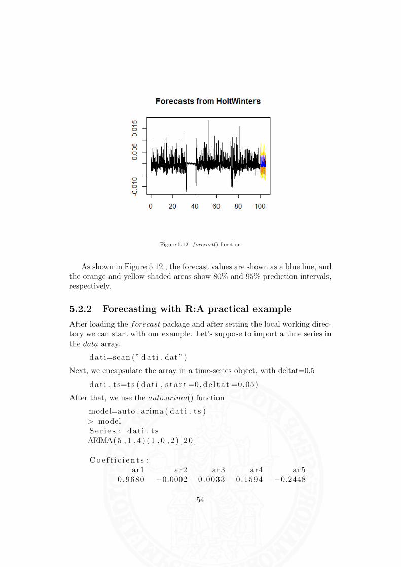
Figure 5.12: forecast() function

As shown in Figure 5.12 , the forecast values are shown as a blue line, andthe orange and yellow shaded areas show 80% and 95% prediction intervals,respectively.

5.2.2 Forecasting with R:A practical example

After loading the forecast package and after setting the local working direc-tory we can start with our example. Let’s suppose to import a time series inthe data array.

da t i=scan (” da t i . dat ”)

Next, we encapsulate the array in a time-series object, with deltat=0.5

da t i . t s=t s ( dat i , s t a r t =0, d e l t a t =0.05)

After that, we use the auto.arima() function

model=auto . arima ( da t i . t s )> modelS e r i e s : da t i . t sARIMA( 5 , 1 , 4 ) ( 1 , 0 , 2 ) [ 2 0 ]

C o e f f i c i e n t s :ar1 ar2 ar3 ar4 ar5

0 .9680 −0.0002 0 .0033 0 .1594 −0.2448

54

s . e . 0 .0232 0 .0349 0 .0352 0 .0320 0 .0217ma1 ma2 ma3 ma4

−0.0355 −0.0327 −0.0342 0 .8322s . e . 0 .0155 0 .0196 0 .0158 0 .0105

sar1 sma1 sma2−0.4231 −0.1819 −0.3245

s . e . 0 .1692 0 .1665 0 .1034

sigma ˆ2 est imated as 1325 : l og l i k e l i h o o d =−12041.83AIC=24109.66 AICc=24109.81 BIC=24184.84

then we make a forecast with prediction horizon h=100 and then we plot theresults in Figure 5.13:

da t i . f o r e c a s t=f o r e c a s t ( model , h=100)p l o t ( da t i . f o r e c a s t )

Figure 5.13: forecast() function with auto.arima()

55

Chapter 6

Comparison of differenttechniques

6.1 Testbed

6.1.1 Data Sets

Data sets are obtained from Heterogenous Networks Data Traces and Mag-Nets data traces Sections of GRID Unina Website [119] and from SANETNetworks data traces Section of SANET website [122]

Heterogenous Networks Data Traces Section contains data traces fromreal networks obtained using D-ITG [120]. Each archive is in tar.gz for-mat and contains files with samples of measured QoS parameters related toseveral end-to-end paths. The considered QoS parameters are packet loss,delay, and jitter. Samples are obtained by adopting an active measurementapproach, sending probe packets by using D-ITG with a packet rate of 100pps. File names have the following format:

xxx-to-yyy-ttll[-ddee]-ppp.tar.gz

where:

• xxx= Access network at sender side (with the term wired we mean 100Mbps Ethernet connection; ADSL is an 640 Kbps connection; with theterm wireless we mean 802.11b connection (ap = access point, ah = adhoc mode))

• yyy= Access network at receiver side (with the term wired we mean100 Mbps Ethernet connection; ADSL is an 640 Kbps connection; with

56

the term wireless we mean 802.11b connection (ap = access point, ah= ad hoc mode))

• tt: Operating System at Sender Side (with the term Win we meanWin32 OS; with the term lin we mean Linux OS)

• ll: Operating System at Receiver Side (with the term Win we meanWin32 OS; with the term lin we mean Linux OS)

• dd: Device at Sender Side (with the term lap we mean laptop; withthe term ws we mean workstation). It is an optional field.

• ee: Device at Receiver Side (with the term lap we mean laptop; withthe term ws we mean workstation). It is an optional field.

• ppp: Used Protocol (TCP, UDP, or SCTP)

Each archive contains several files with the indication of the:

• used packet size (64, 512, 1024 bytes)

• measured QoS parameter (packet loss, delay, or jitter).

Each sample is calculated using non-overlapping windows of 10ms length.In this test following packages are used with 64 bytes packet size :

• gprs-to-wired-winlin-tcp.log.tar.gz

• gprs-to-wired-winlin-udp.log.tar.gz

As example, Figure 6.1 shows the representation of gprs-to-wired-winlin-tcp dataset.

MagNets Data Traces Section contains data traces from the MAG-NETS network backbone [121] obtained using D-ITG [120]. The traces havebeen collected during a joint research activity between University of NapoliFederico II and the Network Group of the Deutsche Telekom Laboratories inBerlin. Each archive contains files with samples of QoS parameters measuredover four end-to-end paths. The considered QoS parameters are throughput,packet loss, delay (RTT), and jitter. Samples are obtained, by adopting anactive measurement approach, sending probe packets using two packet rates(128 pps and 11000 pps) and packet size of 1024 Bytes. For each path andfor each QoS parameter, 20 tests have been performed. File names have thefollowing format:

57

Figure 6.1: Gprs-to-wired-winlin-tcp dataset

xxx-to-yyy-ppp.tar.gz

where

• xxx = Sender node

• yyy = Receiver node

• ppp = Packet rate (128 pps or 11000 pps)

Each archive contains several files with the indication of the:

• measured QoS parameter (throughput, packet loss, delay, or jitter);

• used protocol (TCP or UDP);

• iteration number (1 to 20).

Each sample is calculated using non-overlapping windows of 50ms length.In this study Short-Term HHI-TC-11000 TCP and UDP iteration 1 Trace isused.

SANET is an independent civil association, members of which agreedwith conditions to provide each other with Internet services. It is a non-profit organization whose members contribute to operation of the network.SANET is not the organization managed by the Ministry of Education of theSlovak Republic. Data traces are obtained using MRTG [123], a free software

58

for monitoring and measuring the traffic load on network links. MRTG iswritten in Perl and can run on Windows, Linux, Unix, Mac OS and NetWare.It allows the user to see traffic load on a network over time in graphical form.Data traces for this test are taken from Port1 log of website [122] and werelast updated on Wednesday, 22 February 2012 at 11:17, at which time thenetwork ’L2-SIX-KE’ had been up for 396 days, 5:39:46. More infirmationson data trace are written as follows:

• System: UVT TU Kosice

• Interface: GigabitEthernet

• Ip: 192.108.145.10

• Max Speed: 1 Gbit/s

A single data trace is composed by several sub traces:

• Daily traces: sampled every 5 minutes;

• Weekly traces: sampled every 30 hours;

• Monthly traces: sampled every 2 hours;

• Yearly traces: sampled every 1 day;

A better overview with forecasts is showed in Table 6.1

Table 6.1: SANET Data Traces: sampling and forecasts

Period Sampling PredictionHorizon 50 Horizon 100

Day 5m 250m 500mWeek 30m 25h 50hMonth 2h 100h 200hYear 1d 50d 100d

With SANET traces was not possible to make predictions using Holt-Winters models, since the algorithm was crashed.

59

6.1.2 Techniques and Errors

From the point of view of used techniques, the choices for this study areARIMA models, Holt-Winters models, FTDNN and NARX networks. ARIMAand Holt-Winters models performance evaluation are implemented throughR software. ARIMA models are found using function auto.arima() thatautomatically returns best ARIMA model according to either AIC, AICcor BIC value. Holt-Winters models are found using HoltWinters() func-tion whose beta and gamma parameters are determined by minimizing thesquared prediction error. Forecasts are generated with forecast() function.During representation, predicted values are plotted as a blue line, the 80%prediction interval as an orange shaded area, and the 95% prediction intervalas a yellow shaded area. R software is also used to implement componentdecomposition (Section 6.1.3) through the function stl() (see Section 5.2.1).Implementation of Neural Networks issues are made through MatLab andNeural Network Toolbox.

Settings for FTDNN Neural Networks are:

Network s e t t i n g s :t imede laynet with a tapped delay l i n e ( de lay from 1 to H)and 5 neurons in the hidden l a y e r .

Tra in ing s e t t i n g s :ftdnn0 . tra inFcn = ’ t ra inb fg ’ ; % ( t r a i n i n g func t i on )ftdnn0 . d i v i d e f c n =’ ’ ;ftdnn0 . trainParam . epochs = 1000 ; % maximum number o f i t e r a t i o n sftdnn0 . trainParam . time = 300 ; % maximum t r a i n i n g time in secftdnn0 . trainParam . min\ grad = 1e−10; % minimum Gradient Magnitude

Settings for NARX Neural Networks are:

Network s e t t i n g s :narxnet with 5 neurons in each hidden l a y e r .

Tra in ing s e t t i n g s :net . t ra inFcn = ’ t ra inb fg ’ ; % t r a i n i n g func t i onnet . d i v i d e f c n =’ ’ ;net . trainParam . epochs = 1000 ; % maximum number o f i t e r a t i o n snet . trainParam . time = 300 ; % maximum t r a i n i n g time in secnet . trainParam . min\ grad = 1e−10; % minimum Gradient Magnitude

Performance evaluation is made calculating different kinds of error. Thechoice of parameters for this study is for RMSE, MAE, MAPE. RMSE is

60

generally preferred to the MSE as it is on the same scale as the data. His-torically, the RMSE and MSE have been popular, largely because of theirtheoretical relevance in statistical modelling. But they are more sensitivethan MAE to outliers, which has led some authors to recommend againsttheir use in forecast accuracy evaluation. MAPE has the disadvantage ofbeing infinite or undefined if the forecast value is zero. MAE is preferred be-cause it is simpler to explain but it remains a problem making a comparisonbetween time series forecasts that are on different scales. For this reason it’sconvenient to normalize the value of MAE, having the MAEN. In formulas:

MAEN =MAE

max(|{yj}|)=mean(|yj − yj|)max(|{yj}|)

where {yj} is the dataset, yj is the actual value and yj is the predictedvalue. Main advantages of using MAEN are:

• better performance evaluation, compared to the scale of the actualdataset;

• better individuation of techniques that haven’t got good performances,with MAEN values greater than one;

• better comparison between performance of different parameters anddifferent dataset components;

6.1.3 Data set decomposition

In case of MagNets Short-Term HHI-TC-11000 TCP and UDP iteration 1Trace and SANET traces, a decomposition algorithm is used in order toextract main components of a time series zt:

• Tt, the trend component. It reflects the long term progression of theseries;

• St, the seasonal component. It reflects the repetitive and predictablemovement around the trend component;

• et, the remainder component.

This decomposition is made using stl() function in R, described in Section5.2.1, and Matlab. An example of stl() result is shown in Figure 6.2. Incase of MagNets traces the evaluation of seasonal component was excluded,since data values were related to few minutes of sampling. In case of SANETtraces all components were evaluated, since data are referred to differentdays, weeks and months.

61

Figure 6.2: Decomposition of a Time-Series using stl() function in R

6.2 Results and Errors Evaluation

6.2.1 GPRS-to-wired traces

In Table 6.5 are shown the performance metrics related to the short-termtraces obtained from Heterogenous Networks Data Traces.

Let’s do a detailed analysis on the following data packages:

• gprs-to-wired-winlin-tcp.log.tar.gz

• gprs-to-wired-winlin-udp.log.tar.gz

These two Traces are obtained from a gprs access network, with Win32OS at sender side, to a wired access network using Linux OS at receiver side.Both TCP and UDP protocol are traced.

Predictions were made for the Delay, Jitter and Packet Loss parameters.After that, it was extrapolated the MAE performance and then we calculatedthe normalized MAE (MAEN).

62

The resultant MAEN values are shown in Table 6.6 (MAEN TCP forTCP data and MAEN UDP for UDP data). Analyzing this Table and fo-cusing on Delay parameter and FTDNN technique, the worst value occuron prediction horizon H400 UDP. For H=100 we have the best value (SeeFigure 6.3(a) ) and, in general, the best results are associated to the lowerforecast horizon. With NARX technique the worst value is for H400 UDP,while best value is for H400 TCP.(See Figure 6.3(b)). To a greater value offorecast horizon doesn’t corresponds a greater value of MAEN. Performancesaren’t better than FTDNN case. ARIMA technique produce the the worstvalue for H100 UDP and the best result is associated to the higher forecasthorizon. The greater is the forecast horizon, the greater is MAEN value. InHolt-Winters methods, Better MAEN values are registered for H100 UDPcase (See Figure 6.4(a)) and the worst value is for H100 TCP. However per-formances are somewhat comparable with ARIMA ones.

Examining the Jitter values (from the same 6.6) table, can be observedthat with the FTDDNN the best result is associated to the lower forecast hori-zon (See Figure 6.5(a)). TCP data prediction seems to be better performedthan UDP data prediction. The worst case is for H400 UDP. With NARX,the worst value is for H400 UDP. Best value, instead, occur for H100 TCP.Order of magnitude of MAEN is the same that in the case of FTD neu-ral networks. Observing the obtained ARIMA values , the worst value isfor H100 UDP. Increasing the forecast horizon the obtained MAEN valuesare better. The best value is for H400 TCP. Jitter prediction with Holt-Winters produces the worst value is for H400 TCP. While the best value isfor H100 TCP (See Figure 6.6(a)). Error values are comparable with ARIMAones (See Figure 6.6(b)).

An overall view is seen in table 6.2, we can note some interesting charac-teristics of the prediction performance. In first place, comparing both NeuralNetworks we can see that FTDNN has better performance. Focusing on De-lay parameter is possible to note that there are no substantial differencesusing different prediction horizon (H = 100 or 400), but the best MAEN, in general, are obtained with H=400. Paying attention on Jitter MAENvalues is natural to note that they are lower than which are obtained withDelay ( 10−2 ). The most performing techniques are FTDNN (with H=100)and ARIMA (with H=400) for this parameter. For both Delay and Jitterparameters , in general , in case of TCP transport protocol there is a bet-ter prediction performance than in UDP case. For the Packet Loss, instead,there are no MAEN values because this QoS parameter is always zero inthese two analyzed data packages.

63

(a) PARAM=Delay, PROT=TCP, TECH=FTDNN, H=100

(b) PARAM=Delay, PROT=TCP, TECH=NARX, H=400

Figure 6.3: Prediction plots of Delay with ANN

64

(a) PARAM=Delay, PROT=UDP, TECH=Holt-Winters, H=100

(b) PARAM=Delay, PROT=TCP, TECH=ARIMA, H=400

Figure 6.4: Prediction plots of Delay with Holt-Winters and ARIMA65

(a) PARAM=Jitter, PROT=TCP, TECH=FTDNN, H=100

(b) PARAM=Jitter, PROT=TCP, TECH=NARX, H=100

Figure 6.5: Prediction plots of Jitter with ANN

66

(a) PARAM=Jitter, PROT=TCP, TECH=Holt-Winters, H=100

(b) PARAM=Jitter, PROT=TCP, TECH=ARIMA, H=400

Figure 6.6: Prediction plots of Jitter with Holt-Winters and ARIMA67

Table 6.2: GPRS-to-wired trace MAEN Discussion

GPRS-to-wired trace MAEN DiscussionFTDNN NARX ARIMA H-W

TCP UDP TCP UDP TCP UDP TCP UDPDelay H100 X X

H400 X XJitter H100 X X X

H400 X

6.2.2 MagNets Network

Regarding the MagNets data traces, following packages are used :

• HHI-TC-11000 TCP and UDP.

As said in the section 6.1.3, the prediction was made for original timeseries and for each component ( Trend and Remainder, Seasonal componentwas excluded because prediction of seasonal time series is very accurate sincethe periodicity). Since the periodical nature of seasonal component, andsince the duration of time series we’re analyzing is few minutes, we ignoredconsiderations about seasonal components and focused on trend and remain-der components. The performance results are shown from Table 6.7 to Table6.13.

Focusing on Table 6.14 and Bitrate parameter, for FTDNN it’s possible tosee that all best values are for H=100. Prediction of Trend (See Figure 6.7(a))has a MAEN lower than the original time series and also remainder, exceptthan in case H=400. In fact, in this case MAEN is greater than 1 (worstvalue of test), that means prediction of FTDNN is not accurate. OriginalTime series and Remainder component of Time Series have the same order ofMAEN. Moreover, TCP results are generally better than UDP results. ForNARX techniques (See Figure 6.7(b)), in general, all H=400 prediction casesare well performed. The worst value comes with UDP Reminder and H=100.Best values are registered for Trend TCP/UDP prediction cases. RegardingARIMA techniques, best performance are in original time series for UDP case(See Figure 6.8(b)) and trend time series for TCP case. Only in original timeseries and UDP case, increasing the forecast horizon we can see a MAEN 4times lower. Most cases of best performances are in H100 configurations. Fi-nally for Holt-Winters algorithm, in most cases H100 configurations producesbetter results. In H400 trend prediction, both tcp and udp produces resultsgreater than 1, that means the procedure has not good performances. In thesame Table 6.14, relating to Delay parameter, for FTDNN it’s possible to see

68

(a) PARAM=Bitrate, COMPONENT=Trend, PROT=TCP,TECH=FTDNN, H=100

(b) PARAM=Bitrate, COMPONENT=Trend, PROT=UDP, TECH=NARX,H=400

Figure 6.7: Prediction plots of Bitrate with FTDNN and NARX

69

(a) PARAM=Bitrate, COMPONENT=All, PROT=UDP,TECH=HoltWinters, H=400

(b) PARAM=Bitrate, COMPONENT=ALL, PROT=UDP,TECH=ARIMA, H=400

Figure 6.8: Prediction plots of Bitrate with Holt-Winters and ARIMA

70

(a) PARAM=Delay, COMPONENT=Trend, PROT=UDP, TECH=FTDNN,H=100

(b) PARAM=Delay, COMPONENT=Trend, PROT=TCP, TECH=NARX,H=100

Figure 6.9: Prediction plots of Delay with FTDNN and NARX

71

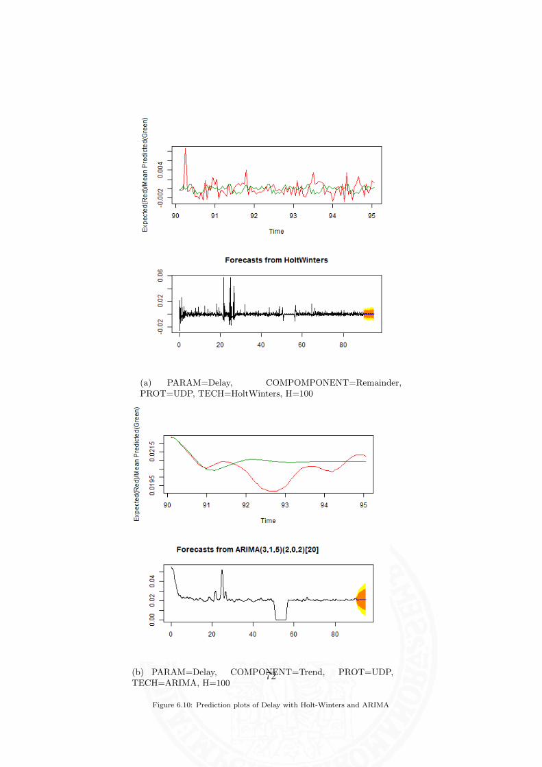
(a) PARAM=Delay, COMPOMPONENT=Remainder,PROT=UDP, TECH=HoltWinters, H=100

(b) PARAM=Delay, COMPONENT=Trend, PROT=UDP,TECH=ARIMA, H=100

Figure 6.10: Prediction plots of Delay with Holt-Winters and ARIMA

72

that best performances are in trend prediction (See Figure 6.9(a)), in par-ticular in UDP case. In some cases H400 case has better performance thanH100 case, while the worst performance are in TCP Remainder prediction.For TCP data, almost best values occur with horizon 100. In contrast withUDP cases, in which all best MAEN are registered with an horizon of 400(See Figure 6.9(b)). For ARIMA techniques (See Figure 6.10(b)), all the bestperformance are in H100 case, except in trend TCP case, in which differencewith H100 is not big. In case of TCP remainder and original Time Series,MAEN is greater than one. Error in case H400 is greater than H100. InHolt-Winters algorithm, all best performance are in H100 case. Best result(See Figure 6.10(a)) is in UDP case, for remainder component.

Focusing on Table 6.15 and Jitter parameter, for FTDNN it’s possibleto see that all best values occur for H=100. Trend prediction performanceseems to be the best among the other components and the whole time-series.Note that for H=400 all TCP components provide Normalized MAE valuesgreater than ”1”, as occur also for UDP Season component. So FTDNNis not accurate for H400 for this parameter. With NARX techniques, bestvalue is for forecast horizon 100, Trend component and TCP protocol (SeeFigure 6.11(b)). In ARIMA section, some values are greater than ”1”. Overall the best MAEN values are registered for H=400 in TCP time series andwith UDP Reminder component (See Figure 6.12(b)), while for Holt-Wintersmodel the best values occur for H=400. In general we have good values withH=100. In the same Table 6.15, relating to Packet Loss Parameter with UDPtransport protocol (in case of TCP, Packet Loss is zero), for FTDNN it’s pos-sible to see that MAEN values are better for H=100 (See Figure 6.13(a)).With NARX techniques, the best value is for the Trend component and withH=100 (See Figure 6.13(b)). For all other component performances are ina lower level. Regarding ARIMA models, the best value occurs for Trendcomponent and H=100 (See Figure 6.14(b)). All the other values are 1 or 2orders greater than the best value, while for Holt-Winters models there aregood values with H=100 (See Figure 6.14(a)). For an overall point of view,from the Table 6.14 and Table 6.15 can be argued that, generally, in caseof UDP transport protocol there are better prediction performances, exceptthe case of NARX neural networks in which best performances are reachedwith TCP transport protocol. Prediction on Trend component and remain-der component has better performances than original time series, except thecase of Bitrate parameter. Forecast horizon H=100 is the best case for al-most all the tests. Learning based techniques have better performances inprediction of the trend component. Since trend component is more smoothedthan remainder and original time series, we could expect these results. The

73

(a) PARAM=Jitter, COMPONENT=Trend, PROT=UDP, TECH=FTDNN,H=100

(b) PARAM=Jitter, COMPONENT=Trend, PROT=TCP, TECH=NARX,H=100

Figure 6.11: Prediction plots of Jitter with FTDNN and NARX

74

(a) PARAM=Jitter, COMPONENT=Remainder, PROT=UDP,TECH=HoltWinters, H=400

(b) PARAM=Jitter, COMPONENT=Remainder, PROT=UDP,TECH=ARIMA, H=400

Figure 6.12: Prediction plots of Jitter with Holt-Winters and ARIMA

75

(a) PARAM=Packet Loss, COMPONENT=Trend, PROT=UDP,TECH=FTDNN, H=100

(b) PARAM=Packet Loss, COMPONENT=Trend, PROT=UDP,TECH=NARX, H=100

Figure 6.13: Prediction plots of Packet Loss with FTDNN and NARX

76

(a) PARAM=Packet Loss, COMPONENT=Remainder,PROT=UDP, TECH=HoltWinters, H=400

(b) PARAM=Packet Loss, COMPONENT=ALL, PROT=UDP,TECH=ARIMA, H=400

Figure 6.14: Prediction plots of Packet Loss with Holt-Winters and ARIMA

77

Packet Loss parameter is always zero for the TCP protocol, so there aren’trelated performance values. Table 6.3 gives an overview of the techniquesthat produce the best MAEN values for each parameter.

Table 6.3: MagNet Short Term best MAEN overview

MagNet Short Term MAEN DiscussionFTDNN NARX ARIMA H-W

TCP UDP TCP UDP TCP UDP TCP UDPBitrate All X X X

Trend XRemainder

Delay AllTrend X X XRemainder X

Jitter AllTrend X X XRemainder X

PacketLoss All O O O OTrend O X O X O X ORemainder O O O O X

6.2.3 SANET Network

Regarding SANET Network, overall performance with different kinds of er-rors are showed in Tables 6.16, 6.17, 6.18, 6.19.

As showed in evaluation table 6.20, in Day trace and FTDNN neuralnetworks it’s possible to see that the best result is for trend trace and lowestforecast horizon (See figure 6.15(a)). We can expect this result becausethe trend evolves with small variations and his pattern is generally simplerto predict. Also in NARX case the best results are in prediction of trendtrace (See figure 6.15(b)). In case of ARIMA models, performance on trendare lower than ones calculated with neural networks technologies, but thebetter performance are with remainder with lowest forecast horizon (Seefigure 6.15(c))

Regarding Week trace in table 6.20 and FTDNN neural networks, bestresults are with trend and lower forecast horizon (See figure 6.16(a)). Gen-erally increasing of forecast horizon makes a growing of MAEN. FTDNN arethe best. Also in NARX case, best results are for trend trace and for lowerforecast horizon (See figure 6.16(b)). In case of ARIMA models, predictionon trend trace (that has the best value, as seen in figure 6.16(c)) has theworst results than NARX and FTDNN.

78

(a) TRACE=Day, H=50, COMP=Trend,TECH=FTDNN

(b) TRACE=Day, H=100, COMP=Trend,TECH=NARX

(c) TRACE=Day, H=50, COMP=Remainder,TECH=ARIMA

Figure 6.15: Link Load Prediction over a Gigabit Ethernet of COMP component of TRACE dataset withTECH technique and H Horizon

79

(a) TRACE=Week, H=50, COMP=Trend,TECH=FTDNN

(b) TRACE=Week, H=50, COMP=Trend,TECH=NARX

(c) TRACE=Week, H=50, COMP=Trend,TECH=ARIMA

Figure 6.16: Link Load Prediction over a Gigabit Ethernet of COMP component of TRACE dataset withTECH technique and H Horizon

80

Regarding Month trace in table 6.21, in FTDNN the best values (see figure6.17(a)) are substantially obtained for H50. The worst value is for Remaindercomponent with H100. Trend component prediction is the best performed.Also in NARX case Trend component prediction shown the best value butthis time for H100 (See figure 6.17(b)). The worst value occur for Remaindercomponent with H100. In ARIMA models all the best MAEN values areregistered for H50. The relative best value is for Remainder prediction, asseen in figure 6.17(c).

Regarding Year trace in table 6.21, for FTDNN the best values are gener-ally obtained for H50 (See figure 6.18(a)). The worst value is for Remaindercomponent with H100. Trend component prediction is the best performed.Results comparable with the FTDNN ones’ obtained for monthly data. InNARX neural networks, the best value is for Trend with H50 (see figure6.18(b)). However, in general prediction is well performed in case of H100.In ARIMA case, the best value is for the original time series with H50 (seefigure 6.18(c)). Comparing these results with FTDNN and NARX we notethat Neural Networks perform better than ARIMA.

As overall evaluation, as seen in figure 6.4, it is possible to say thatFTDNN and NARX neural networks have better performance in trend com-ponent prediction. We can expect this result because the trend evolves withsmall variations and his pattern is generally simpler to predict. In FTDNNcase study, better performance are with lower forecast horizon, except thecase of seasonal component, in which the best results are reached with higherforecast horizon. It’s a good trick to see not only the values of MAEN, butalso the way in which the techniques produces a pattern, that follows the realplot of data traces. From this point of view, with Neural Networks resultsobtained are very accurate, while ARIMA results are not performing well.

81

(a) TRACE=Month, H=50, COMP=Trend,TECH=FTDNN

(b) TRACE=Month, H=100, COMP=Trend,TECH=NARX

(c) TRACE=Month, H=50, COMP=Remainder,TECH=ARIMA

Figure 6.17: Link Load Prediction over a Gigabit Ethernet of COMP component of TRACE dataset withTECH technique and H Horizon

82

(a) TRACE=Year, H=50, COMP=Trend,TECH=FTDNN

(b) TRACE=Year, H=50, COMP=Trend,TECH=NARX

(c) TRACE=Year, H=50, COMP=ALL,TECH=ARIMA

Figure 6.18: Link Load Prediction over a Gigabit Ethernet of COMP component of TRACE dataset withTECH technique and H Horizon

83

Table 6.4: SANET Link Load MAEN Discussion

SANET MAEN DiscussionFTDNN NARX ARIMA

Day AllSeasonTrend X XRemainder X

Week AllSeasonTrend X X XRemainder

Month AllSeasonTrend X XRemainder X

Year All XSeasonTrend X XRemainder

6.3 Results and Evaluation tables

In this section, for a better consultation, a list of tables related to the per-formance metrics is showed.

84

Table 6.5: GPRS-to-wired-winlin TCP and UDP Error Results

TCP

Parameter Technique Forecast RMSE MAE MAPE MAENHorizon

Delay FTDNN 400 9.64E+02 3.94E+02 6.89E+01 8.19E-02100 7.58E+02 3.15E+02 6.08E+01 6.56E-02

NARX 400 1.00E+03 4.21E+02 9.55E+01 8.75E-02100 9.94E+02 5.07E+02 9.43E+01 1.05E-01

ARIMA 400 9.97E+02 4.12E+02 Inf 8.55E-02100 1.05E+03 4.37E+02 Inf 9.09E-02

Holt-Winters 400 1.01E+03 4.07E+02 Inf 8.46E-02100 1.10E+03 4.45E+02 Inf 9.25E-02

Jitter FTDNN 400 2.96E-02 7.40E-03 9.90E+01 2.27E-04100 6.00E-03 4.50E-03 8.71E+01 1.38E-04

NARX 400 2.96E-02 7.43E-03 9.86E+01 2.28E-04100 6.77E-03 5.47E-03 8.44E+01 1.68E-04

ARIMA 400 4.60E-02 5.68E-03 Inf 1.74E-04100 8.67E-02 1.31E-02 Inf 4.01E-04

Holt-Winters 400 4.66E-02 8.74E-03 Inf 8.74E-03100 8.75E-02 1.65E-02 Inf 5.05E-04

PacketLoss PacketLoss is zero in data trace

UDP

Parameter Technique Forecast RMSE MAE MAPE MAENHorizon

Delay FTDNN 400 1.00E+03 5.03E+02 9.21E+01 1.04E-01100 9.43E+02 4.08E+02 9.50E+01 8.48E-02

NARX 400 1.15E+03 6.48E+02 9.48E+01 1.35E-01100 1.07E+03 4.89E+02 9.53E+01 1.02E-01

ARIMA 400 1.02E+03 4.44E+02 Inf 9.23E-02100 1.05E+03 4.64E+02 Inf 9.64E-02

Holt-Winters 400 1.07E+03 4.21E+02 Inf 8.74E-02100 1.01E+03 3.95E+02 Inf 8.20E-02

Jitter FTDNN 400 2.41E-01 1.59E-01 1.06E+02 4.82E-03100 4.14E-02 2.41E-02 9.04E+01 7.32E-04

NARX 400 1.72E+00 1.68E+00 2.14E+02 5.10E-02100 4.18E-02 1.82E-02 9.58E+01 5.52E-04

ARIMA 400 1.43E-01 3.01E-02 Inf 9.15E-04100 2.75E-01 5.04E-02 Inf 1.53E-03

Holt-Winters 400 1.45E-01 2.82E-02 Inf 8.55E-04100 2.75E-01 4.79E-02 Inf 1.45E-03

PacketLoss PacketLoss is zero in data trace

85

Tab

le6.6

:R

esu

lts

from

gp

rs-t

o-w

ired

-win

lin

TC

Pan

dU

DP

Err

or

Evalu

ati

on

Fore

cast

Hori

zon

HM

AE

NT

CP

MA

EN

UD

PD

ela

yF

TD

NN

H100

6.56

E-0

28.

48E

-02

H400

8.19

E-0

21.

04E

-01

Best

Valu

eH

100

H10

0

NA

RX

H100

1.05

E-0

11.

02E

-01

H400

8.75

E-0

21.

35E

-01

Best

Valu

eH

400

H10

0

AR

IMA

H100

9.09

E-0

29.

64E

-02

H400

8.55

E-0

29.

23E

-02

Best

Valu

eH

400

H40

0

H-W

H100

9.25

E-0

28.

20E

-02

H400

8.46

E-0

28.

74E

-02

Best

Valu

eH

400

H10

0

Jit

ter

FT

DN

NH

100

1.38

E-0

47.

32E

-04

H400

2.27

E-0

44.

82E

-03

Best

Valu

eH

100

H10

0

NA

RX

H100

1.68

E-0

45.

52E

-04

H400

2.28

E-0

45.

10E

-02

Best

Valu

eH

100

H10

0

AR

IMA

H100

4.01

E-0

41.

53E

-03

H400

1.74

E-0

49.

15E

-04

Best

Valu

eH

400

H40

0

H-W

H100

5.05

E-0

41.

45E

-03

H400

8.74

E-0

38.

55E

-04

Best

Valu

eH

100

H40

0P

ack

etL

oss

Pac

ketL

oss

isze

roin

the

anal

yze

dti

me

seri

es.

MA

EN

anal

ysi

ssk

ipp

ed.

86

Table 6.7: MagNet Short Term Trace UDP Bitrate Error Results

Magnet Short Term UDP Bitrate Error Results

Technique Forecast Component RMSE MAE MAPE MAENHorizon

FTDNN 100 ALL 4.21E+03 3.26E+03 1.52E+00 1.337E-01Seasonal 1.32E-03 1.14E-03 4.00E-06 1.719E-06

Trend 5.02E+02 3.88E+02 3.82E+00 1.961E-02Remainder 3.53E+03 2.68E+03 7.92E+01 1.808E-01

400 ALL 1.23E+04 9.98E+03 4.28E+01 4.089E-01Seasonal 6.07E-04 5.20E-04 6.00E-06 7.814E-07

Trend 3.64E+04 3.35E+04 2.53E+02 1.696E+00Remainder 4.83E+03 3.80E+03 8.14E+01 2.569E-01

NARX 100 ALL 4.20E+03 3.22E+03 9.22E+00 1.318E-01Seasonal 3.79E+02 2.98E+02 7.81E+01 4.476E-01

Trend 5.76E+02 4.66E+02 3.39E+00 2.355E-02Remainder 8.15E+03 6.99E+03 8.95E+01 4.718E-01

400 ALL 3.62E+03 2.85E+03 3.15E+00 1.167E-01Seasonal 3.35E+02 2.77E+02 8.71E+01 4.159E-01

Trend 1.59E+02 1.18E+02 9.55E-03 5.956E-03Remainder 3.57E+03 2.80E+03 9.08E+01 1.893E-01

ARIMA 100 ALL 3.91E+03 2.97E+03 6.92E+01 1.216E-01Seasonal error error error

Trend 8.17E+02 6.22E+02 9.14E+00 3.143E-02Remainder 3.52E+03 2.63E+03 1.12E+02 1.774E-01

400 ALL 7.84E+03 1.39E+01 6.03E+01 5.693E-04Seasonal error error error

Trend 6.50E+03 5.35E+03 3.76E+01 2.703E-01Remainder 3.69E+03 2.94E+03 1.03E+02 1.982E-01

HoltWinters 100 ALL 4.80E+03 3.46E+03 5.82E+01 1.417E-01Seasonal 2.58E-14 1.31E-14 7.79E-15 1.967E-17

Trend 1.31E+04 1.15E+04 1.59E+02 5.813E-01Remainder 3.65E+03 2.63E+03 1.94E+02 1.775E-01

400 ALL 7.16E+02 7.16E+02 1.02E+01 2.933E-02Seasonal 3.28E-14 2.13E-14 1.39E-14 3.203E-17

Trend 4.93E+04 4.34E+04 3.36E+02 2.196E+00Remainder 3.81E+03 3.00E+03 1.78E+02 2.029E-01

87

Table 6.8: Magnet Short Term UDP Delay Error Results

Magnet Short Term UDP Delay Error Results

Technique Forecast Component RMSE MAE MAPE MAENHorizon

FTDNN 100 ALL 5.10E-03 4.20E-03 1.88E+01 3.844E-02Seasonal 3.30E-04 2.58E-04 2.21E+01 3.862E-01

Trend 1.18E-04 9.60E-05 9.72E-02 1.745E-03Remainder 1.57E-03 1.19E-03 9.04E+01 2.064E-02

400 ALL 7.10E-03 5.00E-03 1.18E+00 4.58E-02Seasonal 2.83E-04 2.32E-04 1.60E+00 3.47E-01

Trend 4.64E-03 3.64E-03 1.64E+01 6.61E-02Remainder 3.27E-03 2.78E-03 1.07E+02 4.81E-02

NARX 100 ALL 7.06E-02 6.65E-02 3.11E+02 6.084E-01Seasonal 3.25E-04 2.68E-04 9.82E+01 4.012E-01

Trend 3.48E-02 2.54E-02 2.74E+01 4.614E-01Remainder 1.65E-03 1.29E-03 1.00E+02 2.243E-02

400 ALL 2.70E-03 2.08E-03 3.11E+00 1.906E-02Seasonal 4.16E-04 3.21E-04 4.78E+01 4.805E-01

Trend 1.01E-02 1.01E-02 4.89E+01 1.833E-01Remainder 1.91E-03 1.41E-03 1.03E+02 2.439E-02

ARIMA 100 ALL 2.33E-03 1.94E-03 9.77E+00 1.779E-02Seasonal

Trend 7.86E-04 5.59E-04 2.81E+00 1.016E-02Remainder 1.58E-03 1.16E-03 1.01E+02 2.016E-02

400 ALL 5.09E-03 2.82E-03 1.11E+01 2.585E-02Seasonal error error error

Trend 2.98E-03 1.77E-03 7.02E+00 3.225E-02Remainder 4.21E-03 2.37E-03 1.00E+02 4.102E-02

HoltWinters 100 ALL 3.31E-03 2.86E-03 1.45E+01 2.616E-02Seasonal 1.19E-19 1.06E-19 7.01E-14 1.583E-16

Trend 5.28E-03 4.19E-03 2.04E+01 7.623E-02Remainder 1.76E-03 1.37E-03 1.48E+02 2.377E-02

400 ALL 5.17E-03 3.66E-03 1.60E+01 3.354E-02Seasonal 4.24E-19 3.71E-19 2.42E-13 5.553E-16

Trend 2.73E-02 2.29E-02 9.83E+01 4.162E-01Remainder 4.25E-03 2.41E-03 1.59E+02 4.184E-02

88

Table 6.9: Magnet Short Term UDP Jitter Error Results

Magnet Short Term UDP Jitter Error Results

Technique Forecast Component RMSE MAE MAPE MAENHorizon

FTDNN 100 ALL 1.50E-03 1.10E-03 6.13E+01 4.115E-02Seasonal 2.62E-04 2.13E-04 1.36E+01 6.677E-01

Trend 3.28E-04 2.65E-04 9.35E+00 3.011E-02Remainder 9.85E-04 7.19E-04 1.01E+02 3.910E-02

400 ALL 4.90E-03 3.90E-03 4.67E+01 1.46E-01Seasonal 3.74E-04 3.52E-04 4.11E+01 1.10E+00

Trend 3.58E-03 3.08E-03 1.16E+02 3.50E-01Remainder 2.89E-03 2.21E-03 9.59E+01 1.20E-01

NARX 100 ALL 2.11E-02 2.04E-02 8.36E+02 7.647E-01Seasonal 1.50E-04 1.25E-04 1.03E+02 3.918E-01

Trend 3.49E-04 3.11E-04 1.84E+01 3.533E-02Remainder 9.80E-04 7.18E-04 1.01E+02 3.904E-02

400 ALL 1.96E-03 1.08E-03 4.58E+01 4.037E-02Seasonal 1.55E-04 1.22E-04 1.00E+02 3.824E-01

Trend 5.02E-03 4.89E-03 2.52E+02 5.559E-01Remainder 1.51E-03 6.38E-04 1.03E+02 3.469E-02

ARIMA 100 ALL 1.31E-03 9.94E-04 7.89E+01 3.720E-02Seasonal error error error

Trend 9.48E-04 7.79E-04 4.87E+01 8.852E-02Remainder 1.12E-03 8.13E-04 1.08E+02 4.419E-02

400 ALL 1.74E-03 1.42E-03 3.09E+02 5.324E-02Seasonal error error error

Trend 1.87E-03 1.71E-03 2.99E+02 1.945E-01Remainder 1.16E-03 5.52E-04 1.02E+02 3.003E-02

HoltWinters 100 ALL 1.40E-03 1.08E-03 8.45E+01 4.035E-02Seasonal 1.75E-20 1.34E-20 9.24E-14 4.196E-17

Trend 5.62E-03 4.79E-03 2.90E+02 5.438E-01Remainder 1.18E-03 8.50E-04 1.13E+02 4.621E-02

400 ALL 2.02E-03 1.71E-03 3.84E+02 6.408E-02Seasonal 5.26E-20 4.55E-20 3.22E-13 1.428E-16

Trend 2.07E-02 1.81E-02 3.02E+03 2.059E+00Remainder 1.20E-03 6.03E-04 1.78E+02 3.280E-02

89

Table 6.10: Magnet Short Term UDP PacketLoss Error Results

Magnet Short Term UDP Packet Loss Error Results

Technique Forecast Component RMSE MAE MAPE MAENHorizon

FTDNN 100 ALL 1.46E+02 1.11E+02 1.55E+01 5.539E-02Seasonal 2.70E-05 1.70E-05 2.30E-05 6.468E-07

Trend 4.11E+00 3.52E+00 1.55E-02 6.301E-03Remainder 1.39E+02 1.03E+02 7.99E+01 7.111E-02

400 ALL 2.58E+02 1.78E+02 5.27E-01 8.916E-02Seasonal 3.10E+00 2.04E+00 1.25E+01 7.780E-02

Trend 2.30E+01 1.90E+01 8.85E-01 3.408E-02Remainder 2.41E+02 1.73E+02 1.04E+02 1.196E-01

NARX 100 ALL 1.37E+02 1.03E+02 1.36E+01 5.155E-02Seasonal 1.56E+03 1.32E+03 1.31E+03 5.027E+01

Trend 2.06E+00 1.61E+00 1.97E-01 2.893E-03Remainder 1.96E+02 1.51E+02 1.08E+02 1.048E-01

400 ALL 1.62E+02 9.71E+01 1.06E+01 4.855E-02Seasonal 3.95E+01 3.19E+01 5.51E+01 1.215E+00

Trend 1.52E+02 8.81E+01 9.12E+01 1.578E-01Remainder 1.06E+02 1.03E+02 2.19E+01 7.145E-02

ARIMA 100 ALL 2.17E+02 1.60E+02 6.26E+01 7.993E-02Seasonal error error error

Trend 5.91E+00 4.60E+00 9.01E-01 8.245E-03Remainder 2.15E+02 1.59E+02 1.60E+02 1.103E-01

400 ALL 1.57E+02 1.11E+02 5.71E+01 5.546E-02Seasonal

Trend 3.99E+01 3.29E+01 7.19E+00 5.899E-02Remainder 1.50E+02 9.45E+01 1.15E+02 6.548E-02

HoltWinters 100 ALL 2.28E+02 1.73E+02 7.09E+01 8.679E-02Seasonal 4.38E-15 3.94E-15 6.57E-14 1.499E-16

Trend 1.22E+02 1.05E+02 2.07E+01 1.879E-01Remainder 2.20E+02 1.63E+02 1.56E+02 1.129E-01

400 ALL 3.06E+02 2.66E+02 1.14E+02 1.331E-01Seasonal 1.53E-14 1.34E-14 2.33E-13 5.100E-16

Trend 4.85E+02 4.23E+02 9.12E+01 7.581E-01Remainder 1.67E+02 1.22E+02 4.06E+02 8.455E-02

90

Table 6.11: MagNet Short Term TCP Bitrate Error Results

Magnet Short Term TCP Bitrate Error Results

Technique Forecast Component RMSE MAE MAPE MAENHorizon

FTDNN 100 ALL 1.970E+03 1.572E+03 1.572E+03 6.81E-02Seasonal 2.780E-04 2.160E-04 1.900E-05 8.11E-07

Trend 2.234E+02 1.971E+02 3.388E-01 9.97E-03Remainder 1.719E+03 1.370E+03 6.210E+01 1.17E-01

400 ALL 2.625E+03 2.037E+03 5.376E+00 8.82E-02Seasonal 1.257E-03 9.130E-04 1.390E-04 3.43E-06

Trend 9.537E+02 8.756E+02 5.053E+00 4.43E-02Remainder 1.870E+03 1.455E+03 5.543E+01 1.24E-01

NARX 100 ALL 4.006E+03 3.336E+03 1.366E+01 1.44E-01Seasonal 3.314E+02 1.901E+02 4.593E+01 7.14E-01

Trend 5.658E+02 4.613E+02 2.696E-01 2.33E-02Remainder 2.501E+03 1.953E+03 8.370E+01 1.67E-01

400 ALL 2.471E+03 1.975E+03 6.065E+00 8.55E-02Seasonal 7.465E+01 6.186E+01 2.166E+01 2.32E-01

Trend 4.374E+02 3.171E+02 1.052E+00 1.60E-02Remainder 2.556E+03 2.149E+03 1.072E+02 1.83E-01

ARIMA 100 ALL 2.907E+03 2.460E+03 1.469E+01 1.06E-01Seasonal error error error

Trend 1.104E+03 9.679E+02 5.603E+00 4.89E-02Remainder 2.338E+03 1.869E+03 9.997E+01 1.60E-01

400 ALL 2.844E+03 2.433E+03 1.472E+01 1.05E-01Seasonal error error error

Trend 1.965E+03 1.625E+03 9.872E+00 8.21E-02Remainder 2.263E+03 1.856E+03 9.999E+01 1.59E-01

HoltWinters 100 ALL 3.174E+03 2.686E+03 1.640E+01 1.16E-01Seasonal 4.798E-14 4.237E-14 1.221E-13 1.59E-16

Trend 1.098E+04 9.268E+03 5.514E+01 4.69E-01Remainder 2.396E+03 1.926E+03 1.131E+02 1.64E-01

400 ALL 5.061E+03 4.142E+03 2.709E+01 1.79E-01Seasonal 1.685E-13 1.475E-13 4.370E-13 5.54E-16

Trend 4.212E+04 3.651E+04 2.162E+02 1.85E+00Remainder 2.370E+03 1.961E+03 1.492E+02 1.67E-01

91

Table 6.12: MagNet Short Term TCP Delay Error Results

Magnet Short Term TCP Delay Error Results

Technique Forecast Component RMSE MAE MAPE MAENHorizon

FTDNN 100 ALL 1.360E-02 1.100E-02 1.994E+00 2.99E-02Seasonal 0.000E+00 0.000E+00 3.170E-04 0.00E+00

Trend 7.990E-04 6.250E-04 2.350E-01 2.58E-03Remainder 5.404E-03 4.254E-03 1.523E+01 3.43E-02

400 ALL error error errorSeasonal 1.034E-03 8.530E-04 8.565E+00 5.60E-01

Trend 1.646E-02 1.358E-02 1.091E+00 5.60E-02Remainder 1.869E-02 1.488E-02 9.356E+01 1.20E-01

NARX 100 ALL 9.788E-03 7.565E-03 2.055E-01 2.06E-02Seasonal 1.174E-03 9.980E-04 1.066E+02 6.56E-01

Trend 5.570E-04 4.100E-04 8.500E-02 1.69E-03Remainder 7.892E-03 6.171E-03 3.354E+01 4.97E-02

400 ALL 1.154E-02 9.298E-03 1.259E-01 2.53E-02Seasonal 9.150E-04 7.650E-04 7.974E+01 5.02E-01

Trend 4.052E-02 3.317E-02 2.376E+00 1.37E-01Remainder 1.361E-02 1.021E-02 9.568E+01 8.22E-02

ARIMA 100 ALL 1.812E-02 1.388E-02 6.653E+00 3.77E-02Seasonal error error error

Trend 1.023E-02 8.113E-03 4.122E+00 3.34E-02Remainder 1.316E-02 1.078E-02 1.016E+02 8.68E-02

400 ALL 2.025E-02 2.248E+00 7.441E+00 6.11E+00Seasonal error error error

Trend 9.777E-03 7.650E-03 3.804E+00 3.15E-02Remainder 1.380E-02 1.004E+02 1.004E+02 8.08E+02

HoltWinters 100 ALL 2.216E-02 1.820E-02 9.168E+00 4.95E-02Seasonal 5.30E-20 3.54E-20 6.21E-14 2.33E-17

Trend 9.550E-03 1.842E+00 3.813E+00 7.59E+00Remainder 1.851E-02 1.099E+02 2.456E+02 8.85E+02

400 ALL 5.871E-02 4.921E-02 2.486E+01 1.34E-01Seasonal 1.771E-19 1.510E-19 1.816E-13 9.92E-17

Trend 1.432E-02 1.143E-02 5.457E+00 4.71E-02Remainder 3.440E-02 2.935E-02 5.948E+02 2.36E-01

92

Table 6.13: MagNet Short Term TCP Jitter Error Results

Magnet Short Term TCP Jitter Error Results

Technique Forecast Component RMSE MAE MAPE MAENHorizon

FTDNN 100 ALL 3.461E-04 2.729E-04 9.207E+00 4.29E-02Seasonal 1.000E-06 1.000E-06 2.527E-01 2.19E-02

Trend 1.300E-05 1.100E-05 5.120E-01 3.12E-03Remainder 1.270E-04 9.900E-05 8.157E+01 2.44E-02

400 ALL errorSeasonal 1.200E-05 1.000E-05 2.041E+01 2.19E-01

Trend 3.620E-04 3.330E-04 3.477E+01 9.46E-02Remainder 4.030E-04 2.970E-04 9.807E+01 7.31E-02

NARX 100 ALL 2.07E-04 1.780E-04 1.012E+01 2.80E-02Seasonal 2.20E-05 1.900E-05 1.007E+02 4.16E-01

Trend 8.70E-05 7.100E-05 5.527E+00 2.02E-02Remainder 1.30E-04 1.000E-04 9.164E+01 2.46E-02

400 ALL 1.94E-04 1.670E-04 8.675E+00 2.62E-02Seasonal 2.30E-05 1.900E-05 9.743E+01 4.16E-01

Trend 1.23E-03 1.195E-03 1.278E+02 3.39E-01Remainder 1.59E-04 1.250E-04 1.075E+02 3.08E-02

ARIMA 100 ALL 1.812E-02 1.388E-02 6.653E+00 2.18E+00Seasonal 0.00E+00

Trend 7.160E-05 6.432E-05 6.931E+00 1.83E-02Remainder 1.479E-04 1.105E-04 3.302E+02 2.72E-02

400 ALL 1.816E-04 1.575E-04 1.759E+01 2.47E-02Seasonal error error error

Trend 1.757E-04 1.485E-04 1.540E+01 4.22E-02Remainder 1.438E-04 1.115E-04 1.578E+02 2.74E-02

HoltWinters 100 ALL 2.216E-02 1.820E-02 9.168E+00 2.86E+00Seasonal 7.980E-22 2.753E-22 3.810E-15 6.03E-18

Trend 3.338E-04 2.825E-04 2.968E+01 8.02E-02Remainder 1.813E-04 1.417E-04 5.793E+02 3.49E-02

400 ALL 2.419E-04 2.091E-04 2.422E+01 3.28E-02Seasonal 1.026E-21 5.209E-22 5.660E-15 1.14E-17

Trend 1.268E-03 1.098E-03 1.163E+02 3.12E-01Remainder 1.776E-04 1.444E-04 7.270E+02 3.56E-02

93

Tab

le6.1

4:

MagN

etS

hort

Ter

mE

rror

Evalu

ati

on

-B

itra

tean

dD

elay

MagNetShort

Term

ErrorEvaluation

–Bitra

te(B

)and

Delay(D

)

Horizon

MAEN

TCP

MAEN

UDP

HALL

Seas.

Tre

nd

Rem.

ALL

Seas.

Tre

nd

Rem.

FTDNN

BH100

6.81

E-2

8.11

E-7

9.97

E-3

1.17

E-1

1.34

E-1

1.72

E-6

1.96

E-2

1.81

E-1

H400

8.82

E-2

3.43

E-6

4.43

E-2

1.24

E-1

4.09

E-1

7.81

E-7

1.70

E+

02.

57E

-1Best

H100

H10

0H

100

H10

0H

100

H40

0H

100

H10

0

NARX

BH100

1.44

E-1

7.14

E-1

2.33

E-2

1.67

E-1

1.32

E-1

4.48

E-1

2.35

E-2

4.72

E-1

H400

8.55

E-2

2.32

E-1

1.60

E-2

1.83

E-1

1.17

E-1

4.16

E-1

5.96

E-3

1.89

E-1

Best

H400

H40

0H

400

H10

0H

100

H10

0H

400

H40

0

ARIM

AB

H100

1.06

E-1

4.89

E-2

1.60

E-1

1.22

E-1

3.14

E-2

1.77

E-1

H400

1.05

E-1

8.21

E-2

1.59

E-1

5.69

E-4

2.70

E-1

1.98

E-1

Best

H400

H10

0H

400

H40

0H

100

H10

0

H-W

BH100

1.14

E-1

1.5

9E-1

64.

69E

-11.

64E

-11.

42E

-11.

97E

-17

5.81

E-1

1.77

E-1

H400

1.76

E-1

5.5

4E-1

61.

85E

+0

1.67

E-1

2.93

E-2

3.20

E-1

72.

20E

+0

2.03

E-1

Best

H100

H10

0H

100

H10

0H

400

H10

0H

100

H10

0

FTDNN

DH100

2.99

E-2

2.58

E-3

3.43

E-2

3.84

E-2

3.86

E-1

1.74

E-3

2.06

E-2

H400

5.60

E-1

5.60

E-2

1.20

E-1

4.58

E-2

3.47

E-1

6.61

E-2

4.81

E-2

Best

H10

0H

100

H10

0H

400

H10

0H

100

NARX

DH100

2.06

E-2

6.56

E-1

1.69

E-3

4.97

E-2

6.08

E-1

4.01

E-1

4.61

E-1

2.24

E-2

H400

2.53

E-2

5.02

E-1

1.37

E-1

8.22

E-2

1.91

E-2

4.81

E-1

1.83

E-1

2.44

E-2

Best

H100

H40

0H

100

H10

0H

400

H40

0H

400

H40

0

ARIM

AD

H100

3.77

E-2

3.34

E-2

8.68

E-2

1.78

E-2

1.02

E-2

2.02

E-2

H400

6.11

E+

03.

15E

-28.

08E

+2

2.59

E-2

3.23

E-2

4.10

E-2

Best

H100

H40

0H

100

H10

0H

100

H10

0

H-W

DH100

4.95

E-2

2.3

3E-1

77.

59E

+0

8.85

E+

22.

62E

-21.

58E

-16

7.62

E-2

2.38

E-2

H400

1.34

E-1

9.9

2E-1

74.

71E

-22.

36E

-13.

35E

-25.

55E

-16

4.16

E-1

4.18

E-2

Best

H100

H10

0H

400

H40

0H

100

H10

0H

100

94

Tab

le6.1

5:

MagN

etS

hort

Ter

mE

rror

Evalu

ati

on

-Jit

ter

an

dP

ack

etL

oss

MagNetShort

Term

ErrorEvaluation

–Jitter(J

)and

Pack

etL

oss

(P)

Horizon

MAEN

TCP

MAEN

UDP

HALL

Seas.

Tre

nd

Rem.

ALL

Seas.

Tre

nd

Rem.

FTDNN

JH100

4.2

9E-2

2.1

9E-2

3.12

E-3

2.44

E-2

4.12

E-2

6.68

E-1

3.01

E-2

3.91

E-2

H400

2.1

9E-1

9.46

E-2

7.31

E-2

1.46

E-1

1.10

E+

03.

50E

-11.

20E

-1Best

H100

H10

0H

100

H10

0H

100

H10

0H

100

NARX

JH100

2.8

0E-2

4.1

6E-1

2.02

E-2

2.46

E-2

7.65

E-1

3.92

E-1

3.53

E-2

3.90

E-2

H400

2.6

2E-2

4.1

6E-1

3.39

E-1

3.08

E-2

4.04

E-2

3.82

E-1

5.56

E-1

3.47

E-2

Best

H400

H400

H10

0H

100

H40

0H

400

H10

0H

400

ARIM

AJ

H100

2.1

8E+

00.

00E

+0

1.83

E-2

2.72

E-2

3.72

E-2

8.85

E-2

4.42

E-2

H400

2.4

7E-2

4.22

E-2

2.74

E-2

5.32

E-2

1.94

E-1

3.00

E-2

Best

H400

H10

0H

100

H10

0H

100

H40

0

H-W

JH100

2.8

6E+

06.0

3E-1

88.

02E

-23.

49E

-24.

03E

-24.

20E

-17

5.44

E-1

4.62

E-2

H400

3.2

8E-2

1.1

4E-1

73.

12E

-13.

56E

-26.

41E

-21.

43E

-16

2.06

E+

03.

28E

-2Best

H400

H100

H10

0H

100

H10

0H

100

H10

0H

400

FTDNN

PH100

Pack

etLoss

iszero

5.54

E-2

6.47

E-7

6.30

E-3

7.11

E-2

H400

8.92

E-2

7.78

E-2

3.41

E-2

1.20

E-1

Best

H10

0H

100

H10

0H

100

NARX

PH100

5.15

E-2

5.03

E+

12.

89E

-31.

05E

-1H400

4.86

E-2

1.22

E+

01.

58E

-17.

14E

-2Best

H40

0H

400

H10

0H

400

ARIM

AP

H100

7.99

E-2

8.25

E-3

1.10

E-1

H400

5.55

E-2

5.90

E-2

6.55

E-2

Best

H40

0H

100

H40

0H-W

PH100

8.68

E-2

1.50

E-1

61.

88E

-11.

13E

-1H400

1.33

E-1

5.10

E-1

67.

58E

-18.

45E

-2Best

H10

0H

100

H10

0H

400

95

Table 6.16: SANET Day Trace Error Result

SANET Day Trace Error Results

Technique Forecast Component RMSE MAE MAPE MAENHorizon

FTDNN 50 ALL 1.51E+06 1.03E+06 6.26E+00 2.46E-01Seasonal 4.26E+05 3.25E+05 2.47E+01 2.44E-01

Trend 4.55E+05 3.30E+05 1.55E+00 6.48E-02Remainder 4.01E+05 3.10E+05 5.89E+01 4.80E-01

100 ALL 1.92E+06 1.54E+06 2.52E+01 3.67E-01Seasonal 2.39E+05 1.85E+05 7.07E+00 1.38E-01

Trend 1.13E+06 9.53E+05 1.40E+01 1.87E-01Remainder 2.82E+05 2.21E+05 5.30E+01 3.43E-01

NARX 50 ALL 1.54E+06 1.20E+06 2.18E+01 2.85E-01Seasonal 7.65E+05 6.07E+05 7.10E+01 4.55E-01

Trend 2.48E+06 2.08E+06 4.48E+01 4.07E-01Remainder 2.85E+05 2.22E+05 4.91E+01 3.43E-01

100 ALL 1.87E+06 1.31E+06 1.55E+01 3.11E-01Seasonal 6.39E+05 4.48E+05 4.08E+01 3.36E-01

Trend 1.16E+06 8.86E+05 2.16E+01 1.74E-01Remainder 2.86E+05 2.20E+05 6.58E+01 3.40E-01

ARIMA 50 ALL 2.52E+06 2.15E+06 6.77E+02 5.11E-01Seasonal 7.56E+05 6.50E+05 9.16E+01 4.87E-01

Trend 3.41E+06 2.86E+06 5.82E+02 5.62E-01Remainder 1.35E+05 9.51E+04 1.27E+02 1.47E-01

100 ALL 3.00E+06 2.78E+06 9.57E+02 6.61E-01Seasonal 7.29E+05 6.16E+05 9.50E+01 4.62E-01

Trend 3.46E+06 3.16E+06 1.14E+03 6.20E-01Remainder 1.69E+05 1.13E+05 1.13E+02 1.76E-01

96

Table 6.17: SANET Week Trace Error Result

SANET Week Trace Error Results

Technique Forecast Component RMSE MAE MAPE MAENHorizon

FTDNN 50 ALL 1.13E+06 9.09E+05 5.61E+00 1.85E-01Seasonal 3.76E+05 2.88E+05 4.28E+00 1.29E-01

Trend 3.33E+05 2.57E+05 5.68E-01 4.81E-02Remainder 2.77E+05 2.34E+05 6.21E+01 2.34E-01

100 ALL 2.40E+06 1.59E+06 5.05E-01 3.24E-01Seasonal 3.15E+05 2.46E+05 4.17E+00 1.10E-01

Trend 8.83E+05 6.97E+05 9.49E-01 1.31E-01Remainder 4.48E+05 2.69E+05 1.61E+01 2.69E-01

NARX 50 ALL 9.53E+05 7.57E+05 1.71E-01 1.54E-01Seasonal 5.25E+05 4.18E+05 9.27E+00 1.88E-01

Trend 3.30E+05 2.70E+05 1.76E+00 5.05E-02Remainder 2.70E+05 2.23E+05 7.21E+01 2.23E-01

100 ALL 9.25E+05 7.48E+05 7.32E+00 1.53E-01Seasonal 8.50E+05 6.46E+05 5.04E+01 2.91E-01

Trend 1.39E+06 1.12E+06 3.13E+00 2.09E-01Remainder 4.51E+05 3.55E+05 9.52E+01 3.55E-01

ARIMA 50 ALL 1.51E+06 1.21E+06 2.17E+02 2.46E-01Seasonal 9.93E+05 8.35E+05 1.42E+02 3.75E-01

Trend 1.04E+06 8.82E+05 6.15E+01 1.65E-01Remainder 2.89E+05 2.21E+05 9.99E+01 2.21E-01

100 ALL 1.43E+06 1.13E+06 2.00E+02 2.31E-01Seasonal 1.31E+06 1.11E+06 1.20E+02 4.97E-01

Trend 1.64E+06 1.34E+06 3.16E+02 2.52E-01Remainder 2.37E+05 1.76E+05 1.00E+02 1.76E-01

97

Table 6.18: SANET Month Trace Error Result

SANET Month Trace Error Results

Technique Forecast Component RMSE MAE MAPE MAENHorizon

FTDNN 50 ALL 6.49E+05 5.44E+05 6.52E+00 9.17E-02Seasonal 3.44E+05 2.78E+05 4.09E+01 1.80E-01

Trend 1.92E+05 1.60E+05 2.69E+00 3.22E-02Remainder 3.13E+05 2.36E+05 5.31E+01 3.33E-01

100 ALL 8.73E+05 7.08E+05 8.58E-01 1.19E-01Seasonal 2.58E+05 2.11E+05 1.51E+01 1.36E-01

Trend 3.14E+05 2.46E+05 1.52E-02 4.94E-02Remainder 4.55E+05 3.73E+05 6.02E+01 5.26E-01

NARX 50 ALL 7.73E+05 5.93E+05 9.52E+00 1.00E-01Seasonal 4.54E+05 3.46E+05 8.60E+01 2.24E-01

Trend 4.53E+05 3.81E+05 2.27E+00 7.65E-02Remainder 8.47E+05 7.15E+04 7.35E+01 1.01E-01

100 ALL 9.70E+05 7.34E+05 7.72E+00 1.24E-01Seasonal 6.26E+05 5.07E+05 1.23E+02 3.28E-01

Trend 4.58E+05 3.58E+05 2.35E+00 7.20E-02Remainder 3.03E+05 2.40E+05 9.83E+01 3.39E-01

ARIMA 50 ALL 9.04E+05 7.53E+05 4.33E+01 1.27E-01Seasonal 4.62E+05 3.87E+05 1.08E+02 2.50E-01

Trend 1.06E+06 9.15E+05 4.11E+01 1.84E-01Remainder 3.30E+05 8.60E+04 1.11E+02 1.22E-01

100 ALL 9.98E+05 7.96E+05 4.80E+01 1.34E-01Seasonal 5.58E+05 4.39E+05 1.04E+02 2.84E-01

Trend 1.14E+06 9.75E+05 5.75E+01 1.96E-01Remainder 3.23E+05 2.61E+05 1.05E+02 3.69E-01

98

Table 6.19: SANET Year Trace Error Result

SANET Year Trace Error Results

Technique Forecast Component RMSE MAE MAPE MAENHorizon

FTDNN 50 ALL 4.49E+05 3.61E+05 4.07E+00 1.15E-01Seasonal 1.66E+05 1.36E+05 1.56E+01 2.42E-01

Trend 1.16E+05 9.65E+04 1.77E-01 3.83E-02Remainder 1.09E+05 8.71E+04 3.81E+01 2.70E-01

100 ALL 5.67E+05 4.49E+05 7.56E+00 1.43E-01Seasonal 1.36E+05 1.12E+05 1.13E+01 1.98E-01

Trend 1.53E+05 1.28E+05 8.28E-01 5.08E-02Remainder 1.34E+05 1.04E+05 4.44E+01 3.24E-01

NARX 50 ALL 9.53E+05 7.57E+05 1.71E-01 2.40E-01Seasonal 5.25E+05 4.18E+05 9.27E+00 7.42E-01

Trend 3.30E+05 2.70E+05 1.76E+00 1.07E-01Remainder 2.70E+05 2.23E+05 7.21E+01 6.92E-01

100 ALL 9.25E+05 7.48E+05 7.32E+00 2.38E-01Seasonal 8.50E+05 6.46E+04 5.04E+01 1.15E-01

Trend 1.39E+06 1.12E+06 3.13E+00 4.43E-01Remainder 4.51E+05 3.55E+04 9.52E+01 1.10E-01

ARIMA 50 ALL 8.44E+05 7.35E+05 4.41E+01 2.33E-01Seasonal 2.70E+05 2.20E+05 1.43E+02 3.90E-01

Trend 8.96E+05 8.15E+05 4.92E+01 3.24E-01Remainder 1.31E+05 1.05E+05 1.01E+02 3.26E-01

100 ALL 8.58E+05 7.51E+05 4.47E+01 2.39E-01Seasonal 3.02E+05 2.52E+05 1.21E+02 4.47E-01

Trend 8.12E+05 7.39E+05 4.17E+01 2.94E-01Remainder 1.40E+05 1.14E+05 1.00E+02 3.54E-01

99

Table 6.20: SANET Error Evaluation Day and Week Trace

SANET Forecast MAENError Evaluation Horizon H

ALL Season Trend Remainder

Day FTDNN H50 2.46E-01 2.44E-01 6.48E-02 4.80E-01H100 3.67E-01 1.38E-01 1.87E-01 3.43E-01

Best Value H50 H100 H50 H100NARX H50 2.85E-01 4.55E-01 4.07E-01 3.43E-01

H100 3.11E-01 3.36E-01 1.74E-01 3.40E-01Best Value H50 H100 H100 H100

ARIMA H50 5.11E-01 4.87E-01 5.62E-01 1.47E-01H100 6.61E-01 4.62E-01 6.20E-01 1.76E-01

Best Value H50 H100 H50 H50

Week FTDNN H50 1.85E-01 1.29E-01 4.81E-02 2.34E-01H100 3.24E-01 1.10E-01 1.31E-01 2.69E-01

Best Value H50 H100 H50 H50NARX H50 1.54E-01 1.88E-01 5.05E-02 2.23E-01

H100 1.53E-01 2.91E-01 2.09E-01 3.55E-01Best Value H100 H50 H50 H50

ARIMA H50 2.46E-01 3.75E-01 1.65E-01 2.21E-01H100 2.31E-01 4.97E-01 2.52E-01 1.76E-01

Best Value H100 H50 H50 H100

100

Table 6.21: SANET Error Evaluation Month and Year Trace

SANET Forecast MAENError Evaluation Horizon H

ALL Season Trend Remainder

Month FTDNN H50 9.17E-02 1.80E-01 3.22E-02 3.33E-01H100 1.19E-01 1.36E-01 4.94E-02 5.26E-01

Best Value H50 H100 H50 H50NARX H50 1.00E-01 2.24E-01 7.65E-02 1.01E-01

H100 1.24E-01 3.28E-01 7.20E-02 3.39E-01Best Value H50 H50 H100 H50

ARIMA H50 1.27E-01 2.50E-01 1.84E-01 1.22E-01H100 1.34E-01 2.84E-01 1.96E-01 3.69E-01

Best Value H50 H50 H50 H50

Year FTDNN H50 1.15E-01 2.42E-01 3.83E-02 2.70E-01H100 1.43E-01 1.98E-01 5.08E-02 3.24E-01

Best Value H50 H100 H50 H50NARX H50 2.40E-01 7.42E-01 1.07E-01 6.92E-01

H100 2.38E-01 1.15E-01 4.43E-01 1.10E-01Best Value H100 H100 H50 H100

ARIMA H50 2.33E-01 3.90E-01 3.24E-01 3.26E-01H100 2.39E-01 4.47E-01 2.94E-01 3.54E-01

Best Value H50 H50 H100 H50

101

Chapter 7

Conclusion and Future Works

An analysis of the state of the art reveals that the neural network repre-sents the best technology in terms of reliability and prediction accuracy.In fact, in recent years there have been many studies on the various tech-niques that exploit a prediction based learning approach that outperforms,although not overwhelmingly, the various model-based approaches. In addic-tion, learning-based methods are also preferred due the fact that they can betrained directly on data with thousands of inputs and without the need of amathematical model, which is instead necessary in the case of model-basedtechniques such as ARIMA and its variants. In fact, finding a good modelis a very difficult and critical task, since prediction is highly affected by thegoodness of the mathematical model. In this study ARIMA models param-eters are obtained using auto optimization made by R and computed usingmaximum likelihood estimation.

The results obtained by the various tests were analyzed and were cal-culated performance metrics based on square error (RMSE), absolute error(MAE and MAEN) and percentage error (MAPE). In this work, the MAENwas defined as the mean absolute error normalized to the maximum valueof the analyzed time series. Regarding the evaluation of the errors and thusperformance, the MAEN has been chosen, since, being normalized, allowscomparison between different parameters, which may present various datascales, and among various techniques.

Tests performed demonstrate that, in general, the prediction carried outwith a lower forecast horizon (ie, H = 100 for Magnets and heterogeneousnetwork configurations, H = 50 in case of SANET) has better performancecompared to that performed with higher forecast horizon. The best resultsfor end-to-end Delay parameter are obtained predicting UDP protocol dataflows of MagNets network, while for gprs-to-wired dataset best performanceoccur with TCP protocol data flows.

102

Generally, best results occur with time series that present at least a min-imum of seasonality in their patterns. Looking at the plots, we note that thetime series which contain little excursions between successive values, are bet-ter predicted. The increase of the irregularity of time series associated to akey network parameter, causes a degradation of prediction performance andso the plots do not follow well the actual pattern of the time series. For thesereasons the original time series of each parameter is decomposed in seasonal,trend and remainder components, in order to have a better prediction.

Evaluating the computational side we have that, as we already said before,for the model based techniques the task of greater difficulty is to find agood model which models well the time series, while in the case of artificialneural networks, the most critical part is the training of the network thatis time consuming, but this disadvantage is offset by improved predictionperformances.

For the jitter parameter, we have that the results are specular to thoseobtained by the delay. In fact, with gprs-to-wired network configurations wehave better performances in the case of TCP protocol data flows.

Regarding SANET link load prediction, results show good prediction per-formance with lower forecast horizon. In particular, best values in term ofMAEN occur in making prediction of the trend component with FTDNN andNARX techniques. In general, also for SANET, we have best performancewith techniques based on learning.

In conclusion, the techniques of prediction based on a mathematical modelthat reflects the actual pattern of the statistical parameters of the network, donot represent a preferable choice compared to techniques based on learning.This is given by the fact that the network traffic has particular characteristicswhich are badly suited to the modeling by means of standard stochasticmodels. Their chaotic behavior is characterized by sudden periods of highintensity, makes a rigorous and quantitative mathematical treatment difficult.

A list of possible future works that may integrate this work, can be con-stituted by:

• parameter tweaking and retraining to fit well

• data preprocessing aimed to remove outliers;

• try to use the online techniques to perform prediction;

• work on an hybrid prediction method;

• design a custom neural network that integrate the feature of both FTDNN andNARX networks;

• develop a technical specification (new or borrowed from other scientific fields).

103

Bibliography

[1] J. P. Narino-mendoza, B. Donnet, and P. Dupont, “A Comparative Study of Path PerformanceMetrics Predictors,” Methodology, no. 1, pp. 1-4.

[2] U. Rathnayake, M. Ott, and A. Seneviratne, “A DBN approach for network availability prediction,”Proceedings of the 12th ACM international conference on Modeling, analysis and simulation ofwireless and mobile systems - MSWiM ’09, p. 181, 2009.

[3] M. Mirza, J. Sommers, P. Barford, and X. Zhu, “A Machine Learning Approach to TCP ThroughputPrediction,” vol. 18, no. 4, pp. 1026-1039, 2010.

[4] L. J. Chen, C. F. Chou, and B. C. Wang, “A machine learning-based approach for estimatingavailable bandwidth,” in TENCON 2007-2007 IEEE Region 10 Conference, 2007, pp. 1–4.

[5] P. Cortez, M. Rocha, J. Machado, J. Neves, T. Neural, and N. Nn, “A neural network based timeseries forecasting system,” In Practice.

[6] M. Khashei, S. Rezahejazi, and M. Bijari, “A new hybrid artificial neural networks and fuzzyregression model for time series forecasting,” Fuzzy Sets and Systems, vol. 159, no. 7, pp. 769-786,Apr. 2008.

[7] M. Elsabroulj, M. Borrchard, and T. Aboulnasr, “A NEW HYBRID LONG-TERM AND SHORT-TERM PREDICTION ALGORITHM FOR PACKET LOSS ERASURE OVER IP-NETWORKS,”Technology, pp. 361-364.

[8] E. Feng , Min, “A new hybrid model for time-series prediction,” 2009 8th IEEE InternationalConference on Cognitive Informatics, pp. 281-286, Jun. 2009.

[9] L. Xiang, X.-hu Ge, C. Liu, L. Shu, and C.-xiang Wang, “A New Hybrid Network Traffic PredictionMethod 2,” Communications Society, 2010.

[10] Z. Li, Q. Lei, X. Kouying, and Z. Xinyan, “A Novel BP Neural Network Model for Traffic Predictionof Next Generation Network,” 2009 Fifth International Conference on Natural Computation, pp.32-38, 2009.

[11] M. T. Afshar and M. T. Manzuri, “A Novel Technique to Control the Traffic of Wireless Ad-hoc Network by Fuzzy Systems and Prediction with Neural Network,” 2011 Third InternationalConference on Computational Intelligence, Modelling Simulation, pp. 18-21, Sep. 2011.

[12] I. Miloucheva, J. Haringer, S. Iii, and A. Anzaloni, “A practical approach to forecast Quality ofService parameters considering outliers,” Time, 2003.

[13] C. Lee and H. Abe, “A Proposal for Improving Network Throughput Predictability over the Inter-net,” Computing, pp. 2-3, 2009.

[14] X. Wang and X. Shan, “A wavelet-based method to predict Internet traffic,” Analysis, pp. 690-694,2002.

104

[15] Riedmiller, “Advanced Supervised Learning in Multilayer Per- ceptrons - from Backpropagation toAdaptive Learning Techniques,” International Journal of Computer Standards and Interfaces, vol.16, 1994.

[16] T. Liangrui and W. Wenjin, “An improved algorithm based on network load prediction for 802 .11 DCF,” Electronic Engineering, pp. 1466-1469, 2011.

[17] K. M. Rezaul and V. Grout, “An Overview of Long-range Dependent Network Traffic Engineeringand Analysis : Characteristics , Simulation , Modelling and Control,” Traffic Engineering, p. 10,2007.

[18] S. Chabaa, A. Zeroual, and J. Antari, “ANFIS method for forecasting internet traffic time series,”2009 Mediterrannean Microwave Symposium (MMS), pp. 1-4, Nov. 2009.

[19] B. Krithikaivasan, Y. Zeng, K. Deka, and D. Medhi, “ARCH-Based Traffic Forecasting and DynamicBandwidth Provisioning for Periodically Measured Nonstationary Traffic,” IEEE/ACM Transac-tions on Networking, vol. 15, no. 3, pp. 683-696, Jun. 2007.

[20] S. Tabhaw, “Autoregressive, Moving Average and Mixed Autoregressive- Moving Average Processesfor Forecasting QoS in Ad Hoc Networks for real-Time Service Support,” Network, 2004.

[21] F. Puente, C. a. H. S., and O. J. S. P., “Comparative analysis of time series techniques ARIMA andANFIS to forecast Wimax traffic,” Proceedings of the 7th International Conference on Advancesin Mobile Computing and Multimedia - MoMM ’09, p. 277, 2009.

[22] M. Shepperd and G. Kadoda, “Comparing Software Prediction Techniques Using Simulation,” vol.27, no. 11, pp. 1014-1022, 2001.

[23] J. Jiang and S. Papavassiliou, “Detecting Network Attacks in the Internet via Statistical NetworkTraffic Normality Prediction,” Journal of Network and Systems Management, vol. 12, no. 1, pp.51-72, Mar. 2004.

[24] M. Meng, X. Ye, and J. Gu, “End-to-End Delay Boundary Prediction Using Maximum EntropyPrinciple (MEP) for Internet-Based Teleoperation,” Engineering, no. May, pp. 2701-2706, 2002.

[25] G. Iannello and A. Pescap, “End-to-End Packet-Channel Bayesian Model applied to HeterogeneousWireless Networks,” Communications Society, pp. 484-489, 2005.

[26] N. Hu, S. Member, P. Steenkiste, and S. Member, “Evaluation and Characterization of Available,”vol. 21, no. 6, pp. 879-894, 2003.

[27] J. W. Mickens, B. D. Noble, and A. Arbor, “Exploiting Availability Prediction in DistributedSystems,” Symposium A Quarterly Journal In Modern Foreign Literatures, pp. 73-86, 2006.

[28] A. Eswaradass, X.-he Sun, and M. Wu, “A Neural Network Based Predictive Mechanism for Avail-able Bandwidth”.

[29] W. D. Blair and R. Jana, “Forecast Service for Internet Protocol Networks . Approved for PublicRelease,” Components.

[30] P. Cortez, M. Rio, P. Sousa, and M. Rocha, “Forecasting Internet Traffic by Neural Networks UnderUnivariate and Multivariate Strategies,” Network.

[31] N. C. Anand and C. Scoglio, “GARCH - Non-Linear Time Series Model for Traffic Modeling andPrediction,” Traffic, pp. 694-697, 2008.

[32] T. Yensen, S. Member, J. P. Lariviere, I. Lambadaris, and R. A. Goubran, “HMM Delay PredictionTechnique for VoIP,” vol. 5, no. 3, pp. 444-457, 2003.

[33] S. Chabaa, “Identification and Prediction of Internet Traffic Using Artificial Neural Networks,”Journal of Intelligent Learning Systems and Applications, vol. 2, no. 3, pp. 147-155, 2010.

105

[34] a. G. Parlos, “Identification of the Internet end-to-end delay dynamics using multi-step neuro-predictors,” Proceedings of the 2002 International Joint Conference on Neural Networks. IJCNN’02(Cat. No.02CH37290), pp. 2460-2465, 2002.

[35] A. W. Moore and D. Zuev, “Internet Traffic Classification Using Bayesian Analysis TechniquesCategories and Subject Descriptors,” Traffic.

[36] P. Cortez, M. Rio, M. Rocha, and P. Sousa, “Internet Traffic Forecasting using Neural Networks,”The 2006 IEEE International Joint Conference on Neural Network Proceedings, pp. 2635-2642,2006.

[37] Q. Li, D. L. Mills, and S. Member, “Jitter-Based Delay-Boundary Prediction of Wide-Area Net-works,” October, vol. 9, no. 5, pp. 578-590, 2001.

[38] C. Ling, J. Wang, C. Wang, and X. Peng, “Load Balancing Algorithm Based on Time SeriesPrediction of Packet Loss Rate,” Topology, pp. 145-149, 2009.

[39] T. Zhang, E. van den Berg, J. Chennikara, P. Agrawal, and T. Kodama, “Local predictive resourcereservation for handoff in multimedia wireless IP networks,” IEEE Journal on Selected Areas inCommunications, vol. 19, no. 10, pp. 1931-1941, 2001.

[40] V. Bui, W. Zhu, and A. Pescap, “Long Horizon End-to-End Delay Forecasts : A Multi-Step-AheadHybrid Approach,” pp. 825-832.

[41] D. C. Papagiannaki K., Taft N. , Zhang Z., “Long-Term Forecasting of Internet Backbone Traffic.”2005.

[42] J. Chou, B. Lin, S. Sen, and O. Spatscheck, “Minimizing collateral damage by proactive surgeprotection,” Proceedings of the 2007 workshop on Large scale attack defense - LSAD ’07, p. 97,2007.

[43] S. Belhaj and M. Tagina, “Modeling and Prediction of the Internet End-to-end Delay using Recur-rent Neural Networks,” Journal of Networks, vol. 4, no. 6, pp. 528-535, Aug. 2009.

[44] N. Sadek and A. Khotanzad, “Multi-scale high-speed network traffic prediction using k-factorGegenbauer ARMA model,” 2004 IEEE International Conference on Communications (IEEE Cat.No.04CH37577), vol. 0, no. c, pp. 2148-2152 Vol.4, 2004.

[45] M. Swany and R. Wolski, “Multivariate Resource Performance Forecasting in the Network WeatherService †,” Cluster Computing, 2002.

[46] a. Eswaradass, “Network bandwidth predictor (NBP): a system for online network performance fore-casting,” Sixth IEEE International Symposium on Cluster Computing and the Grid (CCGRID’06),p. 4 pp.-268, 2006.

[47] Y. D. Barve, “Neural Network Approach to the Prediction of Percentage Data Packet Loss forWireless Sensor Networks,” Training, pp. 103-106, 2009.

[48] G. Rutka, “Neural Network Models for Internet Traffic Prediction,” Electrical Engineering, vol. 4,no. 4, pp. 55-58, 2006.

[49] G. Tech, “On the Predictability of Large Transfer TCP Throughput *,” Work.

[50] W. E. Leland, M. S. Taqqu, W. Willinger, and D. V. Wilson, “On the self-similar nature of Ethernettraffic (extended version),” IEEE/ACM Transactions on Networking, vol. 2, no. 1, pp. 1-15, 1994.

[51] H. Mehrvar and M. Soleymani, “Packet loss rate prediction using a universal indicator of traffic,”in Communications, 2001. ICC 2001. IEEE International Conference on, 2001, vol. 3, pp. 647–653.

[52] S. Rossi, A. F. Atiya, S. G. Yoo, K. T. Chong, and H. Kim, “Packet Loss Rate Prediction Usingthe Sparse Basis Prediction Model,” Chaos, vol. 18, no. 3, pp. 950-954, 2007.

106

[53] W. Tavernier, D. Papadimitriou, D. Colle, M. Pickavet, and P. Demeester, “Packet loss reductionduring rerouting using network traffic analysis,” Telecommunication Systems, Aug. 2011.

[54] M. Yang and X. R. Li, “Predicting End-to-End Delay of the Internet Using Time Series AnalysisAnalysis of the Internet End-to-End Delay Prediction,” Electrical Engineering, pp. 1-15, 2003.

[55] M. Yang, J. Ru, X. R. Li, H. Chen, and A. Bashi, “Predicting Internet End-to-End Delay: AMultiple-Model Approach,” Proceedings IEEE INFOCOM 2006. 25TH IEEE International Con-ference on Computer Communications, vol. 0, no. c, pp. 1-5, Apr. 2006.

[56] X. R. Li, “Predicting internet end-to-end delay: an overview,” Thirty-Sixth Southeastern Sympo-sium on System Theory, 2004. pp. 210-214.

[57] J. R. Votano, M. Parham, L. H. Hall, L. B. Kier, and L. M. Hall, “Predicting packet loss statisticswith hidden Markov models,” Chemistry biodiversity, vol. 1, no. 11, pp. 1829–1841, 2004.

[58] R. Khosla, S. Fahmy, Y. C. Hu, and J. Neville, “Predicting Prefix Availability in the Internet.”

[59] M. Goyal, R. A. Guerin, and R. Guerin, “Predicting TCP Throughput From Non-invasive NetworkSampling Predicting TCP Throughput From Non-invasive Network Sampling,” Communications,vol. 1, no. Infocom, pp. 180-189, 2002.

[60] W. Junsong, W. Jiukun, Z. Maohua, and W. Junjie, “Prediction of internet traffic based on Elmanneural network,” 2009 Chinese Control and Decision Conference, no. 2, pp. 1248-1252, Jun. 2009.

[61] M. Lee, I. Zitouni, Q. Zhou, B. Labs, and L. Technologies, “PREDICTION-BASED PACKETLOSS CONCEALMENT FOR VOICE OVER IP : A STATISTICAL N-GRAM APPROACH,”Communications Society, pp. 2308-2312, 2004.

[62] P. N. Nobile, R. R. F. Lopes, C. E. Moron, and L. C. Trevelin, “QoS Proxy Architecture for RealTime RPC with Traffic Prediction,” 11th IEEE International Symposium on Distributed Simulationand Real-Time Applications (DS-RT’07), pp. 261-267, Oct. 2007.

[63] L. Roychoudhuri and E. S. Al-Shaer, “Real-time packet loss prediction based on end-to-end delayvariation,” IEEE Transactions on Network and Service Management, vol. 2, no. 1, pp. 29-38, Nov.2005.

[64] Y. Li and M. Zhang, “Research on Network Traffic Forecasting Strategy Based on BP NeuralNetwork,” 2009 International Conference on Computational Intelligence and Software Engineering,pp. 1-4, Dec. 2009.

[65] G. Rutka and G. Lauks, “Study on Internet Traffic Prediction Models,” Electrical Engineering, vol.6, no. 6, 2007.

[66] H. Feng and Y. Shu, “Study on network traffic prediction techniques,” Proceedings. 2005 Interna-tional Conference on Wireless Communications, Networking and Mobile Computing, 2005., vol. 2,no. 3, pp. 995-998.

[67] P. Bermolen and D. Rossi, “Support vector regression for link load prediction,” Computer Networks,vol. 53, no. 2, pp. 191-201, Feb. 2009.

[68] M. Qin and R. Zimmermann, “Supporting Guaranteed Continuous Media Streaming in MobileAd-hoc Networks with Link Availability Prediction,” Simulation, pp. 153-156, 2006.

[69] R. Wolski, N. T. Spring, and J. Hayes, “The network weather service : a distributed resourceperformance forecasting service for metacomputing,” Future Generation Computer Systems, vol.15, pp. 757-768, 1999.

[70] P. Cortez, M. Rio, P. Sousa, and M. Rocha, “Topology Aware Internet Traffic Forecasting usingNeural Networks,” Methods, 2006.

107

[71] Y. H. Chan, T. Randhawa, and S. Hardy, “Traffic prediction based access control using differentvideo traffic models in 3G CDMA high speed data networks,” Proceeding of the 2006 internationalconference on Communications and mobile computing - IWCMC ’06, p. 227, 2006.

[72] O. W. W. Yang, “Traffic Prediction Using FARIMA Models,” Time, pp. 3-7, 1999.

[73] X. Wang, Y. Ren, and X. Shan, “WDRLS : A Wavelet-Based On-Line Predictor for NetworkTraffic,” Update, pp. 4034-4038, 2003.

[74] J. S. Malak, M. Mohsenzadeh, and M. A. Seyyedi, “Web Service QoS Prediction Based on MultiAgents,” 2009 International Conference on Computer Technology and Development, pp. 265-269,Nov. 2009.

[75] J. Mao, “Why artificial neural networks?,” Communications, 1996.

[76] I. Railean, C. Stolojescu, S. Moga, and P. Lenca, “WIMAX Traffic Forecasting based on NeuralNetworks in Wavelet Domain,” Journal of Information Technology, 2010.

[77] V.Frost and B. Melamed, ”Traffic modelling for telecommunications networks”, IEEE Comun.Mag., vol 32, pp70-80, mar 1994.

[78] E. Cinlar. Introduction to Stochastic Processes (Englewood Cliffs, NU:Prentice-Hall, 1975)

[79] V. Paxson, S.Floyd, ”Wide Area Traffic: The Failure of Poisson Modeling” IEEE/ACM Transac-tions, Vol.3, June 1995

[80] J. Bolot, “Characterizing end-to-end packet delay and loss in the internet,” Journal of High SpeedNetworks, vol. 2, no. 3, pp. 289-298, September 1993

[81] Maya Yajnik, Sue B. Moon, James F. Kurose, and Donald F. Towsley ”Measurement and modelingof the temporal dependence in packet loss”, in INFOCOM (1), 1999, pp. 345-352

[82] Vern Paxson, ”End-to-end internet packet dynamics” IEEE/ACM Transactions on Networking,vol. 7, no. 3, pp. 277-292, 1999.

[83] V. Vapnik. The Nature of Statistical Learning Theory. Springer, N.Y., 1995. ISBN 0-387-94559-8.

[84] V. Vapnik, S. Golowich, and A. Smola. Support vector method for function approximation, regres-sion estimation, and signal processing. In M. Mozer, M. Jordan, and T. Petsche, editors, Advancesin Neural Information Processing Systems 9, pages 281– 287, Cambridge, MA, 1997. MIT Press.

[85] K.R. Muller, A.J. Smola, G.Ratsch, B.Scholkopf, J.Kholmorgen, V.Vapnik. Predicting Time Serieswith Support Vector Machines.

[86] R. Hecht-Nielsen, “Theory of the backpropagation neural network”, in Neural Networks, 1989.IJCNN., International Joint Conference on, Jun. 1989, pp. 593-605.

[87] W.S. McCulloch and W. Pitts, “A Logical Calculus of Ideas Immanent in Nervous Activity,” Bull.Mathematical Biophysics,Vol. 5,1943, pp. 115-133.

[88] Jain, A.K., Mao, J., 1996. Mohiddin KM. Artificial neural networks: a tutorial. Computer IEEEMarch, p. 31–44.

[89] Jeffrey L. Elman, ”Finding Structure in Time”. Cognitive Science, Vol. 14, No. 2. (1990), pp.179-211.

[90] T. Lin, B. G. Horne, C. L. Giles, How embedded memory in recurrent neural network architectureshelps learning long-term temporal dependencies, Neural Networks 11 (5) (1998) 861-868.

[91] T. Lin, B. G. Horne, P. Tino, C. L. Giles, Learning long-term dependencies in NARX recurrentneural networks, IEEE Transactions on Neural Networks 7 (6)(1996) 1424-1438.

108

[92] A. Erramilli, M. R. D. Veitch, W. Willinger, Self-similar traffic and network dynamics, Procedingsof the IEEE 9 (5) (2002) 800-819.

[93] M. Grossglauser, J. C. Bolot, On the relevance of long-range dependence in network traffic,IEEE/ACM Transactions on Networking 7 (4) (1998) 329-640.

[94] H. Kantz, T. Schreiber, Nonlinear Time Series Analysis, 2nd ed., Cambridge University Press, 2006.

[95] M. Norgaard, O. Ravn, N. K. Poulsen, L. K. Hansen, Neural Networks for Modelling and Controlof Dynamic Systems, Springer, 2000.

[96] S. Chen, S. A. Billings, P. M. Grant, Nonlinear system identification using neural networks, Inter-national Journal of Control 11 (6) (1990) 1191-1214.

[97] K. S. Narendra, K. Parthasarathy, Identification and control of dynamical systems using neuralnetworks, IEEE Transactions on Neural Networks 1 (1) (1990) 4-27.

[98] K. Claffy, G. Polyzos, and H-W. Braun. Measurement Considerations for Assessing UnidirectionalLatencies. Internetworking: Research and Experience, 4(3):121-132, Sep. 1993.

[99] Y.-C. Su, C.-S. Yang, and C.-W. Lee, “The analysis of packet loss pre- diction for Gilbert-modelwith loss rate uplink,” in Inf. Process. Lett., 2004, vol. 90, pp. 155–159.

[100] P. S. Rossi, G. Romano, F. Palmieri, and G. Ianello, “Joint end-to-end loss-delay hidden Markovmodel for periodic UDP traffic over the Internet,” IEEE Trans. Signal Process., vol. 54, no. 2, pp.530–541, Feb. 2006.

[101] L. Roychoudhuri and E. Al-Shaer, “Real-time packet loss prediction based on end-to-end delayvariation,” IEEE Trans. Network Service Manager. , vol. 2, no. 1, Nov. 2005.

[102] S. G. Yoo, K. T. Chong, and S. Y. Yi, “Neural network modeling of transmission rate control factorfor multimedia transmission using the Internet,” in Lecture Notes in Computer Science, ser. 3399.Berlin, Germany: Springer-Verlag, 2005, pp. 851–862.

[103] S. G. Yoo, K. T. Chong, and H. S. Kim, “Development of predictive TFRC with neural network,”in Lecture Notes in Computer Science, ser. 3606. Berlin, Germany: Springer-Verlag, 2005, pp.193–205.

[104] Amir F. Atiya, Sung Goo Yoo, Kil To Chong, and Hyongsuk Kim, Packet Loss Rate PredictionUsing the Sparse Basis Prediction Model.

[105] A. F. Atiya, M. Aly, and A. G. Parlos, “Sparse basis selection: New results and application toadaptive prediction of video source traffic,” IEEE Trans. Neural Netw., vol. 16, no. 5, pp. 1136–1146,Sep. 2005.

[106] David C. Swanson - 2000 - , Signal processing for intelligent sensor systems - Page 237

[107] P.F. Pai, C.S. Lin, A hybrid ARIMA and support vector machines model in stock price forecasting,Omega 33 (2005) 497–505.

[108] K.Y. Chen, C.H. Wang, A hybrid SARIMA and support vector machines in forecasting the pro-duction values of the machinery industry in Taiwan, Expert Systems with Applications 32 (2007)254–264.

[109] G. Armano, M. Marchesi, A. Murru, A hybrid genetic-neural architecture for stock indexes fore-casting, Information Sciences 170 (2005) 3–33.

[110] H. Kim, K. Shin, A hybrid approach based on neural networks and genetic algorithms for detectingtemporal patterns in stock markets, Applied Soft Computing 7 (2007) 569–576.

[111] A. Sharkey, Types of multinet system Proceedings of the Third International Workshop on MultipleClassifier Systems Lecture Notes in Computer Science, 2364, Springer, London, 2002, 108–117.

109

[112] T. Taskaya, M.C. Casey, A comparative study of autoregressive neural network hybrids, NeuralNetworks 18 (2005) 781–789.

[113] A. C. Harvey. Etne Series Models. The MIT Press, Cambridge, Massachusetts, second edition, 1992

[114] Mathworks. (2011). Neural Networks Toolbox: User’s Guide (r2011b). Retrieved September 2011 .

[115] Hagan, M.T., H.B. Demuth, and M.H. Beale, Neural Network Design, Boston, MA: PWS Publish-ing, 1996.

[116] P. Brockwell and R. Davis, Introduction to Time Series and Forecasting: Springer.Appendix D -An ITSM Tutorial, 1996.

[117] The weka official website:http://www.cs.waikato.ac.nz/ml/weka/index.html

[118] ns-2 official web site:http://www.isi.edu/nsnam/ns/

[119] Heterogenous Networks Data Traces:http://www.grid.unina.it/Traffic/Traces/dtraces.phpMagNets data traces:http://www.grid.unina.it/Traffic/Traces/Magnets.php

[120] http://www.grid.unina.it/software/ITG/

[121] Roger P. Karrer, Petros Zerfos, Nischal M. Piratla, “Magnets - A Next Generation Access Network”- Deutsche Telekom Laboratories

[122] http://mrtg.uvt.tuke.sk/192.108.145.1/

[123] The Multi Router Traffic Grapher, http://oss.oetiker.ch/mrtg/

[124] M. Bouzenada, M.C. Batouche and Z. Telli, Neural Network for Object Tracking - Research Article.

[125] Jose M. Menezes, Guilherme A. Barreto, Long-term time series prediction with the NARX network:An empirical evaluation .Neurocomputing In Advances in Neural Information Processing (ICONIP2006).

[126] http://www.mathworks.it/help/techdoc/

[127] S. Makridakis “A Survey of Time Series”, International Statistical Review Vol. 44, No.1 (Apr. 1976)

[128] B. Krithikaivasan, Y. Zeng, K. Deka, and D. Medhi, “ARCH-based Traffic Forecasting and DynamicBandwidth Provisioning for Periodically Measured Nonstationary Traffic”, IEEE/ACM Transac-tions on Networking, vol. 15, no. 3, pp. 683–697, June 2007.

[129] G. Box, G. Jenkins, Time Series Analysis: Forecasting and Control, 2nd ed. Englewood Cliffs, NJ:Prentice-Hall, 1976.

[130] A.Adas: “Traffic Models in BroadBand Networks” IEEE Communications Magazine, pp. 82-89,July 1997.

[131] Chris Chatfield, Mohammad Yar, “Holt-Winters forecasting: some pratical issues”, (School ofMathematical Sciences, University of Bath, United Kingdom)

[132] V.J. Easton, J.H. McColl, ”Statistics Glossary”

[133] Daniel S. Clouse, C. Lee Giles,Bill G. Horne and Garrison W. Cottrell, ”Time-Delay Neural Net-works: Representation and Induction of Finite-State Machines”. IEEE TRANSACTIONS ONNEURAL NETWORKS, VOL. 8, NO. 5, SEPTEMBER 1997

110