Embed Size (px)
Citation preview
Tesi di Laurea
Break-up of inertial aggregatesin turbulent channel flow
Frammentazione di aggregati inerzialiin flusso turbolento
Relatore: Dott. Ing. Cristian Marchioli
Correlatore: Prof. Alfredo Soldati
Candidato: Marco Svettini
UNIVERSITÀ DEGLI STUDI DI UDINEFacoltà di Scienze Matematiche Fisiche e Naturali
CdLS in FISICA COMPUTAZIONALE
Anno Accademico 2011/2012
Premise
What is turbulence?
Turbulent flux characteristics:
• Unstable and unstationary (Reynolds)
• Tridimensional
• Diffusive
• Dissipative (h Kolmogorov l.s.)
• Rotational: w=rot(u)≠0
• Coherent
Jet flow
η= ඨν3ε4 τ= ට
νε
Δx,Δy,Δz < 𝜂 Δt < 𝜏= η2ν
DNS solver req.:
Length scale:
CFL condition:
Random nature of turbulent flow:u = U+u’(Reynolds decomp.)
𝐶𝑖 = 𝑢𝑖 ∙∆𝑡 ∆𝑥𝑖Τ < 0.1
Premise
Aggregate Break-up in Turbulence
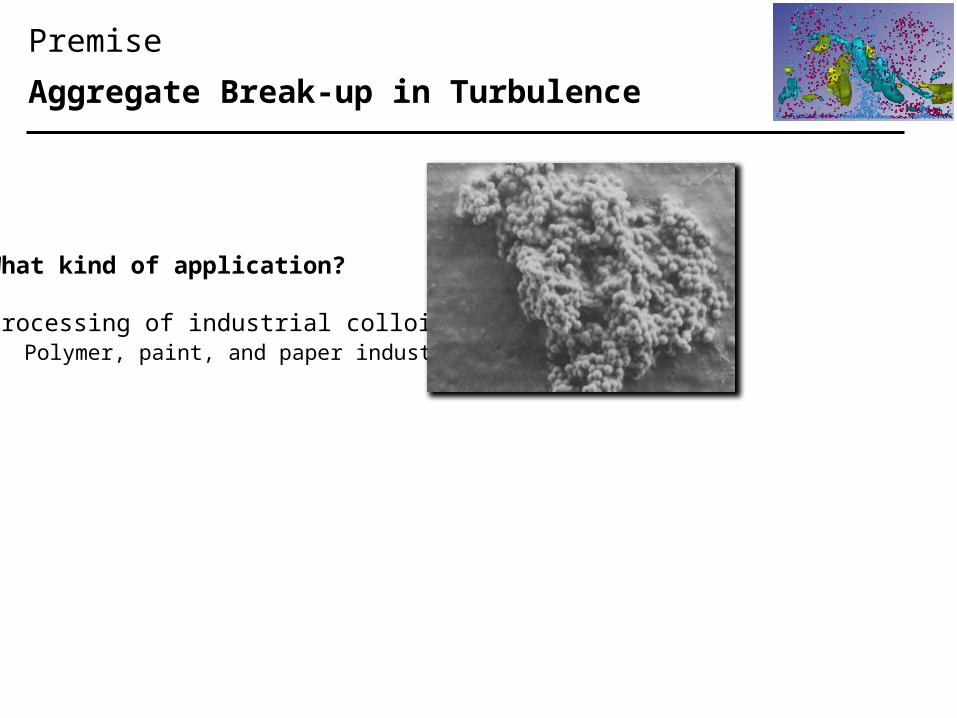
What kind of application?
Processing of industrial colloids• Polymer, paint, and paper industry
Premise
Aggregate Break-up in Turbulence
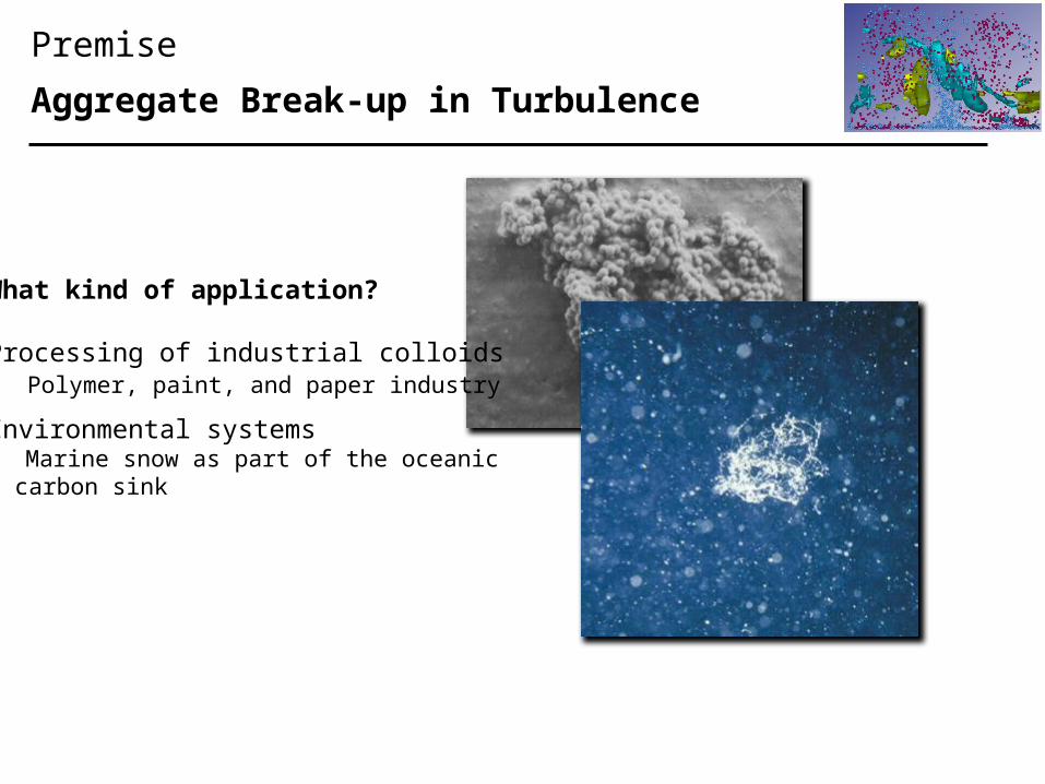
What kind of application?
Processing of industrial colloids• Polymer, paint, and paper industry
Environmental systems• Marine snow as part of the oceanic carbon sink
Premise
Aggregate Break-up in Turbulence
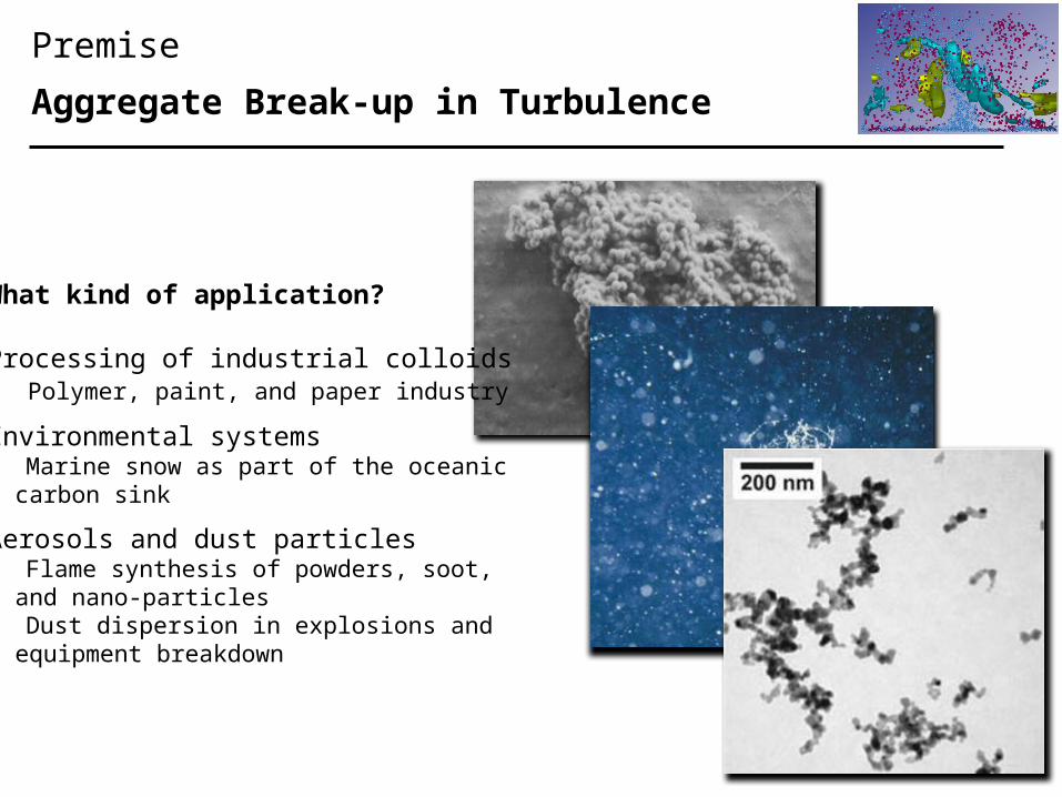
What kind of application?
Processing of industrial colloids• Polymer, paint, and paper industry
Environmental systems• Marine snow as part of the oceanic carbon sink
Aerosols and dust particles• Flame synthesis of powders, soot, and nano-particles• Dust dispersion in explosions and equipment breakdown
Premise
Aggregate Break-up in Turbulence
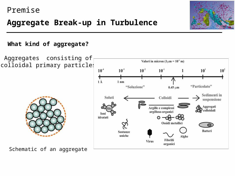
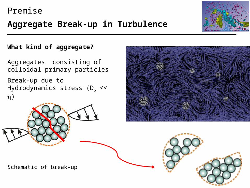
What kind of aggregate?
Aggregates consisting ofcolloidal primary particles
Schematic of an aggregate
What kind of aggregate?
Aggregates consisting ofcolloidal primary particles
Break-up due toHydrodynamics stress (Dp << h)
Schematic of break-up
Premise
Aggregate Break-up in Turbulence
Problem Definition
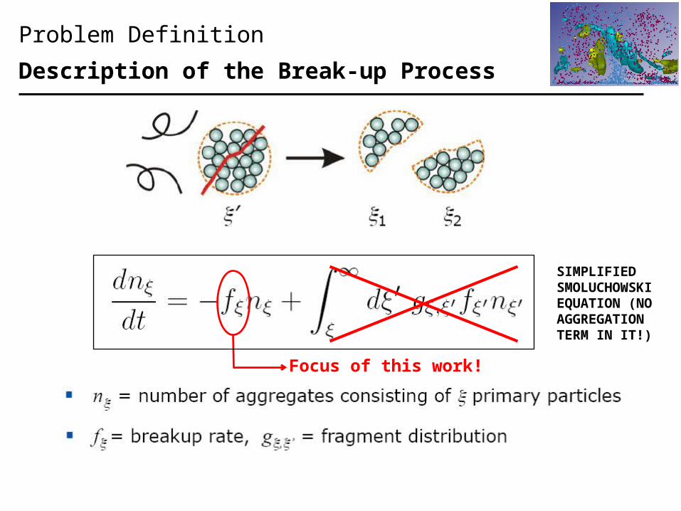
Description of the Break-up Process
Focus of this work!
SIMPLIFIEDSMOLUCHOWSKIEQUATION (NOAGGREGATIONTERM IN IT!)
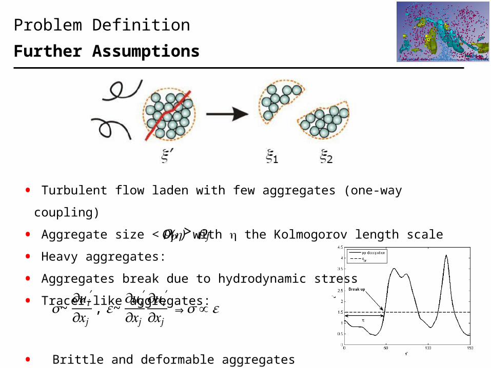
• Turbulent flow laden with few aggregates (one-way coupling)
• Aggregate size < O(h) with h the Kolmogorov length scale
• Heavy aggregates:
• Aggregates break due to hydrodynamic stress
• Tracer-like aggregates:
• Brittle and deformable aggregates
Problem Definition
Further Assumptions
𝜎~𝜕𝑢𝑖′𝜕𝑥𝑗 , 𝜀~𝜕𝑢𝑖′𝜕𝑥𝑗𝜕𝑢𝑖′𝜕𝑥𝑗 ⇒ 𝜎∝ 𝜀
𝜌𝑝 > 𝜌𝑓
Problem Definition
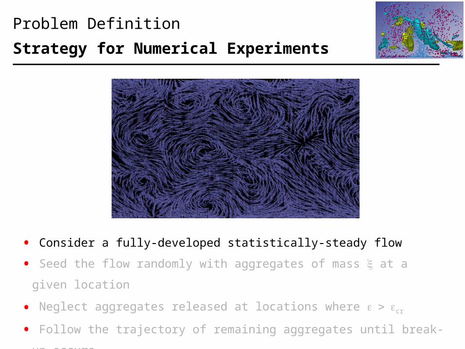
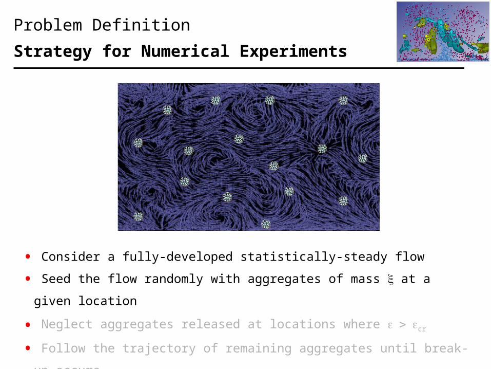
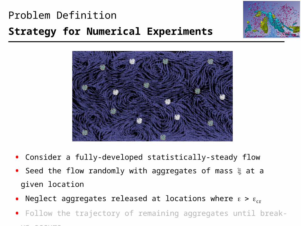
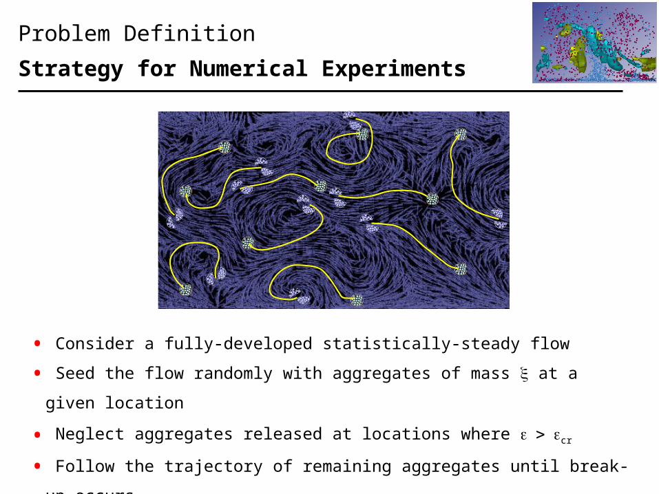
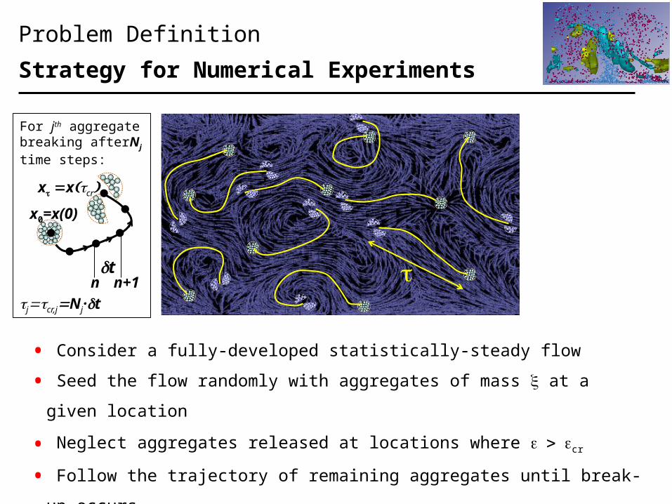
Strategy for Numerical Experiments
• Consider a fully-developed statistically-steady flow
• Seed the flow randomly with aggregates of mass x at a given location
• Neglect aggregates released at locations where > e ecr
• Follow the trajectory of remaining aggregates until break-up occurs
• Compute the exit time, = t tecr (time from release to break-up)
Problem Definition
Strategy for Numerical Experiments
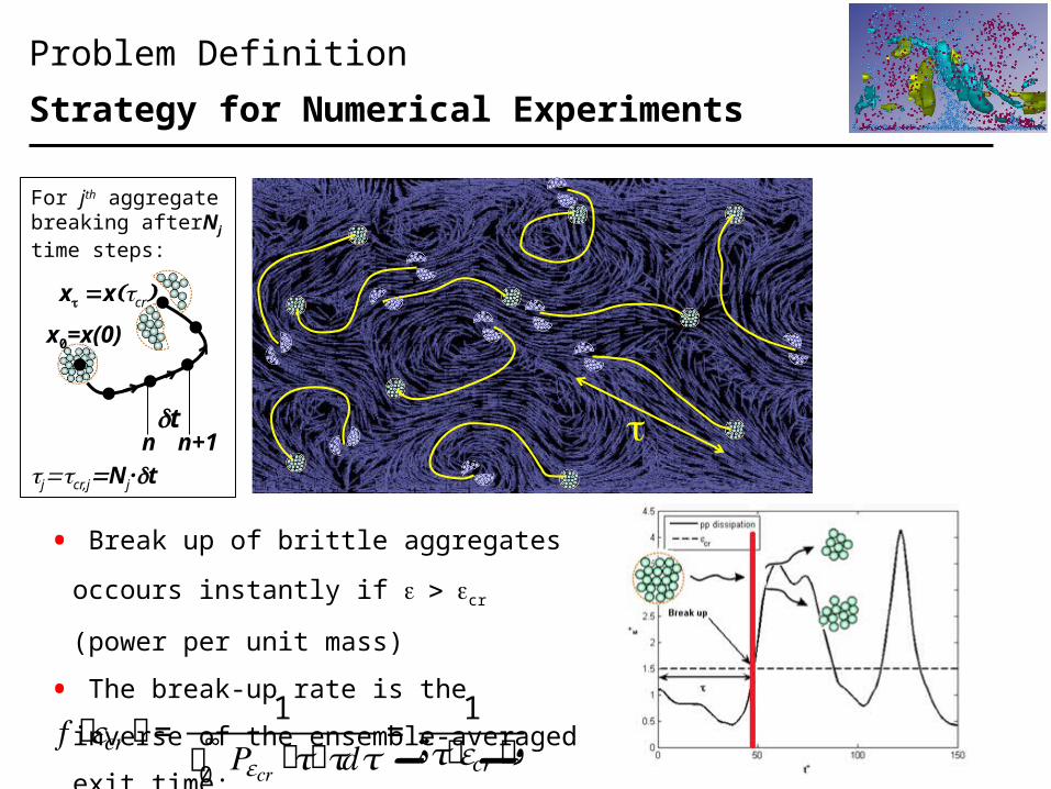
t
For jth aggregatebreaking afterNj
time steps:
x0=x(0)
x t =x(tcr)
dtn n+1
tj=tcr,j=Nj·dt
• Consider a fully-developed statistically-steady flow
• Seed the flow randomly with aggregates of mass x at a given location
• Neglect aggregates released at locations where > e ecr
• Follow the trajectory of remaining aggregates until break-up occurs
• Compute the exit time, = t tecr (time from release to break-up)
Problem Definition
Strategy for Numerical Experiments
• Break up of brittle aggregates occours
instantly if > e ecr (power per unit
mass)
• The break-up rate is the inverse of the
ensemble-averaged exit time:𝑓ሺ𝜀𝑐𝑟ሻ= 1 𝑃𝜀𝑐𝑟ሺ𝜏ሻ∞0 𝜏𝑑𝜏= 1𝜏ሺ𝜀𝑐𝑟ሻۃ ۄ
t
For jth aggregatebreaking afterNj
time steps:
x0=x(0)
x t =x(tcr)
dtn n+1
tj=tcr,j=Nj·dt
Problem Definition
Strategy for Numerical Experiments
• The break-up rate is the inverse of the ensemble-averaged exit time:
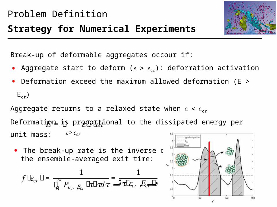
Break-up of deformable aggregates occour if:
• Aggregate start to deform ( > e ecr): deformation activation
• Deformation exceed the maximum allowed deformation (E > Ecr)
Aggregate returns to a relaxed state when < e ecr
Deformation is proportional to the dissipated energy per unit mass:𝐸=න 𝜀ሺ𝑡ሻ𝑑𝑡𝜀>𝜀𝑐𝑟
𝑓ሺ𝜀𝑐𝑟ሻ= 1 𝑃𝜀𝑐𝑟,𝐸𝑐𝑟ሺ𝜏ሻ∞0 𝜏𝑑𝜏= 1𝜏ሺ𝜀𝑐𝑟,𝐸𝑐𝑟ሻۃ ۄ
Flow Instances and Numerical Methodology
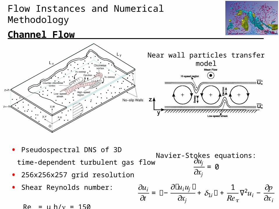
Channel Flow
• Pseudospectral DNS of 3D
time-dependent turbulent gas flow
• 256x256x257 grid resolution
• Shear Reynolds number:
Ret = uth/n = 150
Near wall particles transfer model
Navier-Stokes equations:𝜕𝑢𝑗𝜕𝑥𝑗 = 0 𝜕𝑢𝑖𝜕𝑡 = ቆ−𝜕൫𝑢𝑖𝑢𝑗൯𝜕𝑥𝑗 + 𝛿1𝑖ቇ+ 1𝑅𝑒𝜏∇2𝑢𝑖 − 𝜕𝑝𝜕𝑥𝑖
Particle Tracer and Numerical Methodology
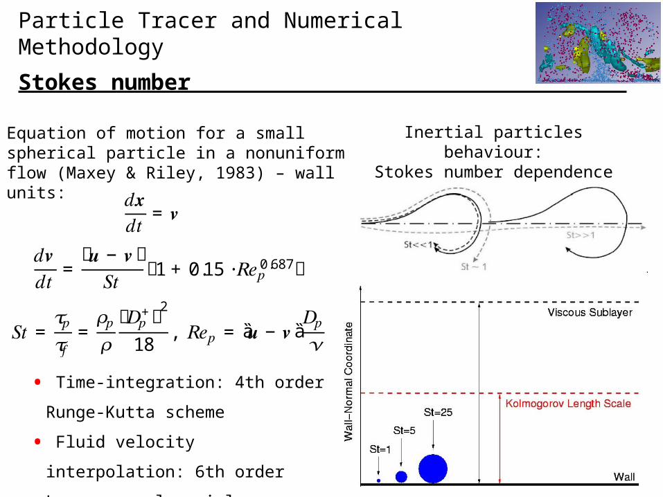
Stokes number
Equation of motion for a small spherical particle in a nonuniformflow (Maxey & Riley, 1983) – wall units:𝑑𝒙𝑑𝑡 = 𝒗
𝑑𝒗𝑑𝑡 = ሺ𝒖− 𝒗ሻ𝑆𝑡 ൫1+ 0.15∙𝑅𝑒𝑝0.687൯ 𝑆𝑡 = 𝜏𝑝𝜏𝑓 = 𝜌𝑝𝜌 ൫𝐷𝑝+൯218 , 𝑅𝑒𝑝 = ȁA𝒖− 𝒗ȁA𝐷𝑝𝜈
• Time-integration: 4th order
Runge-Kutta scheme
• Fluid velocity interpolation: 6th
order Lagrange polynomials
Inertial particles behaviour:Stokes number dependence
Channel Flow
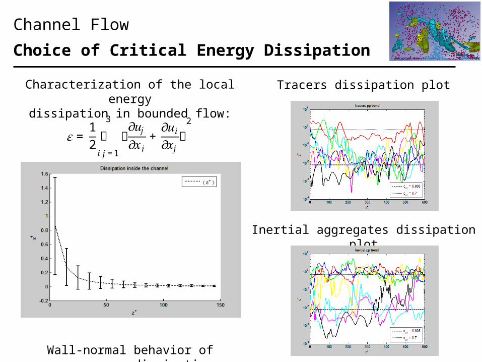
Choice of Critical Energy Dissipation
Characterization of the local energydissipation in bounded flow:
Wall-normal behavior ofmean energy dissipation
𝜀= 12 ቆ𝜕𝑢𝑗𝜕𝑥𝑖 + 𝜕𝑢𝑖𝜕𝑥𝑗ቇ
23𝑖,𝑗=1
Tracers dissipation plot
Inertial aggregates dissipation plot
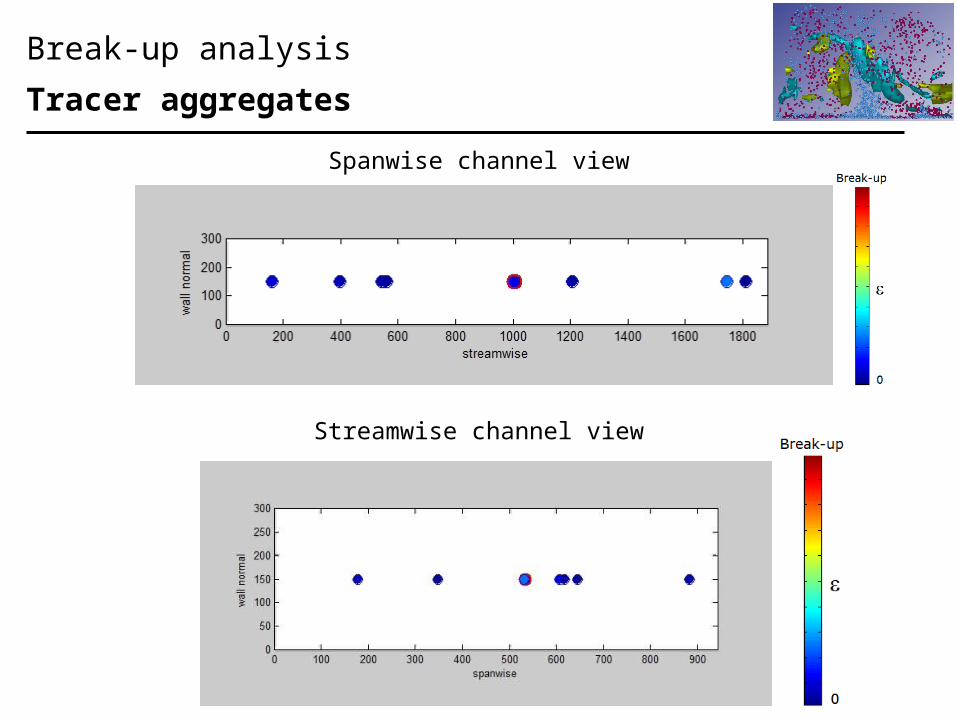
Break-up analysis
Tracer aggregates
Spanwise channel view
Streamwise channel view
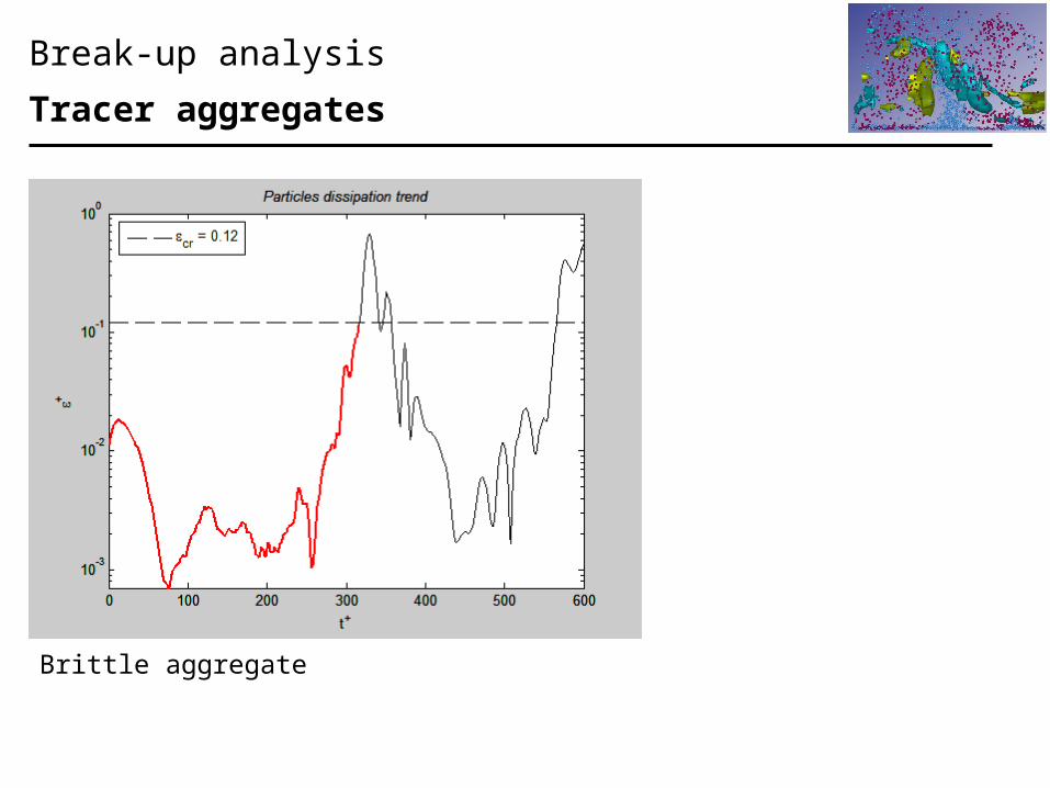
Break-up analysis
Tracer aggregates
Brittle aggregate
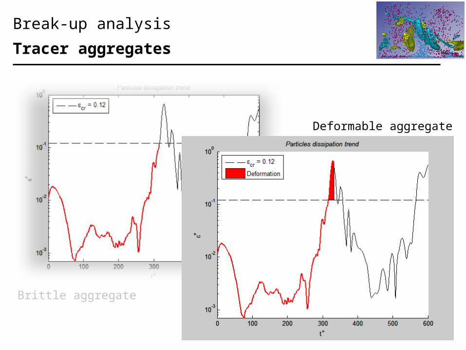
Break-up analysis
Tracer aggregates
Brittle aggregate
Deformable aggregate
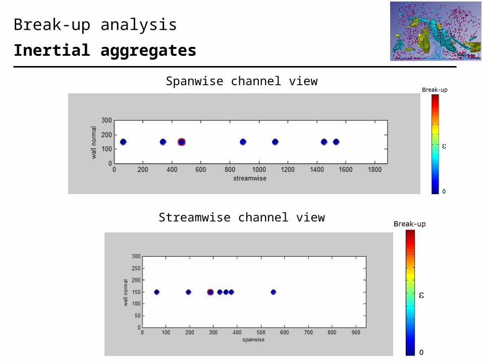
Break-up analysis
Inertial aggregates
Spanwise channel view
Streamwise channel view
Break-up analysis
Inertial aggregates
Brittle aggregate
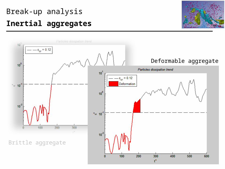
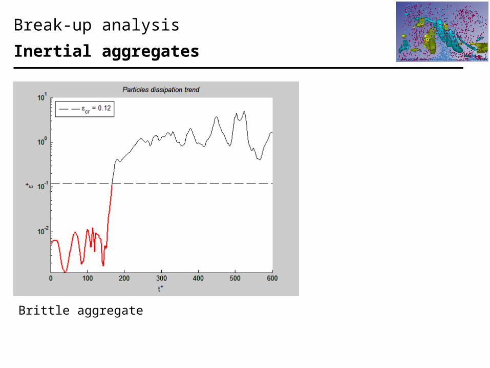
Break-up analysis
Inertial aggregates
Brittle aggregate
Deformable aggregate
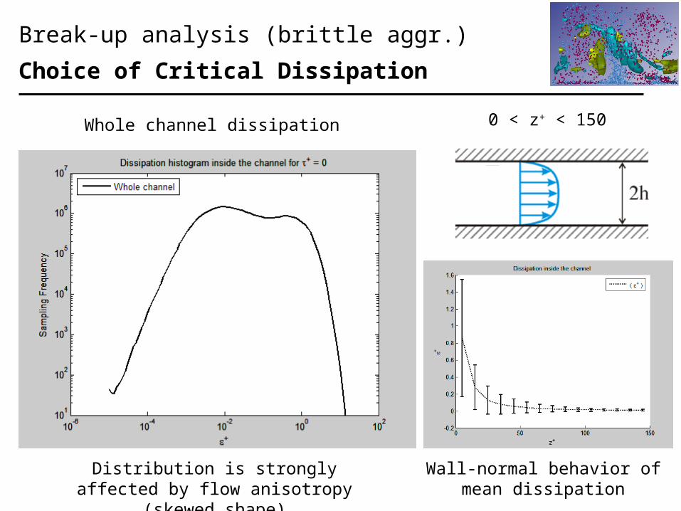
Break-up analysis (brittle aggr.)
Choice of Critical Dissipation
Distribution is strongly affected by flow anisotropy (skewed shape)
Whole channel dissipation
Wall-normal behavior ofmean dissipation
0 < z+ < 150
Break-up analysis (brittle aggr.)
Choice of Critical Dissipation
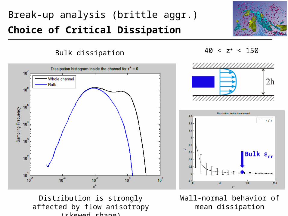
Bulk dissipation
Wall-normal behavior ofmean dissipation
Bulk ecr
Distribution is strongly affected by flow anisotropy (skewed shape)
40 < z+ < 150
Break-up analysis (brittle aggr.)
Choice of Critical Dissipation
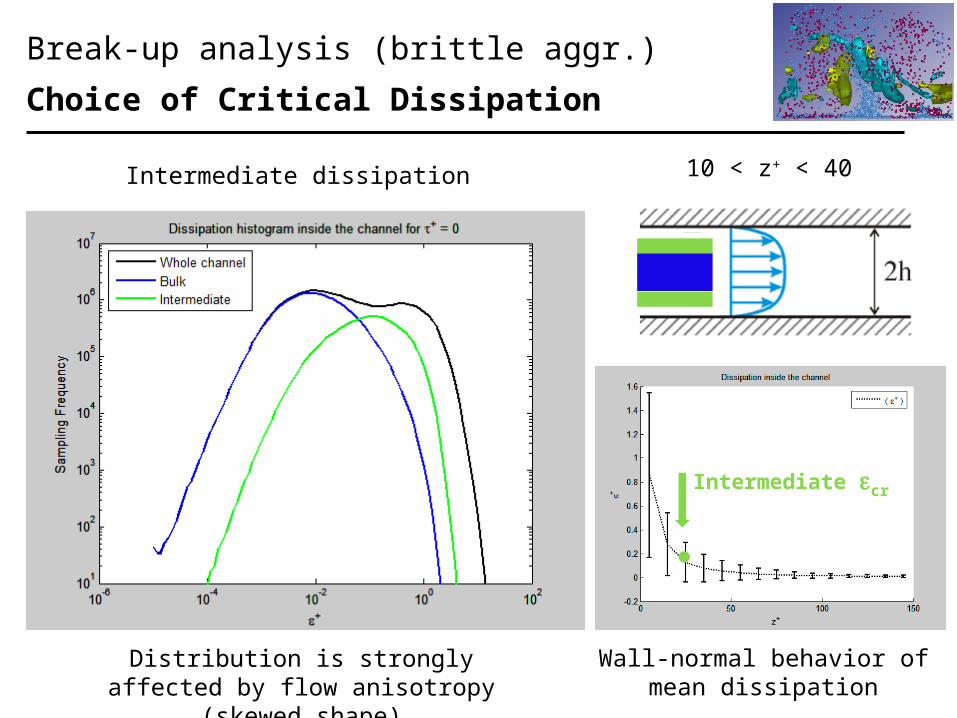
Intermediate dissipation
Wall-normal behavior ofmean dissipation
Intermediate ecr
Distribution is strongly affected by flow anisotropy (skewed shape)
10 < z+ < 40
Break-up analysis (brittle aggr.)
Choice of Critical Dissipation
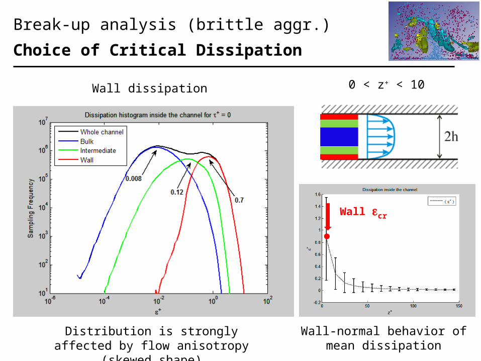
Wall dissipation
Wall-normal behavior ofmean dissipation
Wall ecr
Distribution is strongly affected by flow anisotropy (skewed shape)
0 < z+ < 10
Break-up analysis (brittle aggr.)
Choice of Critical Dissipation
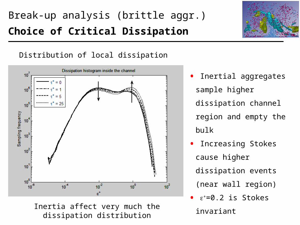
Distribution of local dissipation
Inertia affect very much the dissipation distribution
• Inertial aggregates
sample higher dissipation
channel region and empty
the bulk
• Increasing Stokes cause
higher dissipation events
(near wall region)
• e+=0.2 is Stokes invariant
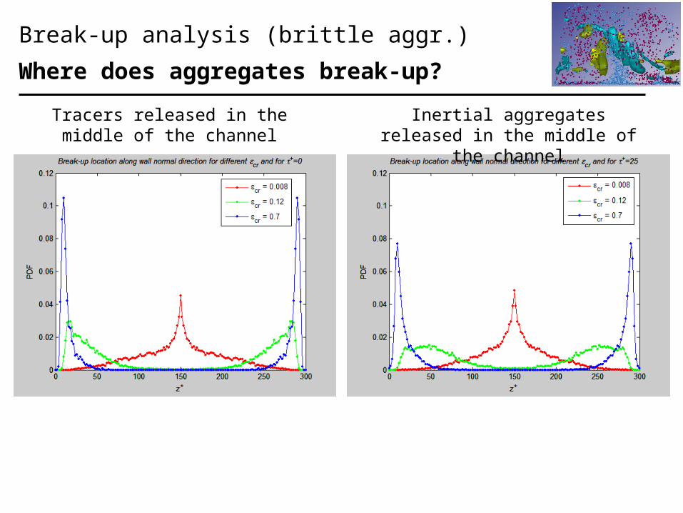
Break-up analysis (brittle aggr.)
Where does aggregates break-up?
Tracers released in themiddle of the channel
Inertial aggregates released in the middle of the channel
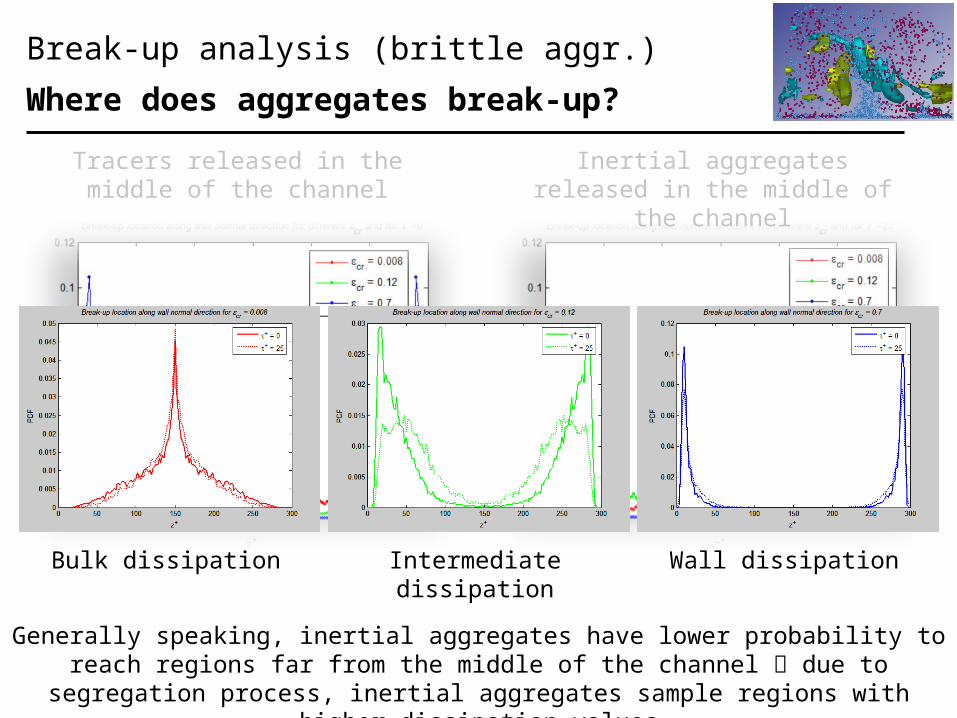
Break-up analysis (brittle aggr.)
Where does aggregates break-up?
Tracers released in themiddle of the channel
Inertial aggregates released in the middle of the channel
Bulk dissipation Intermediate dissipation
Wall dissipation
Generally speaking, inertial aggregates have lower probability to reach regions far from the middle of the channel due to segregation process,
inertial aggregates sample regions with higher dissipation values
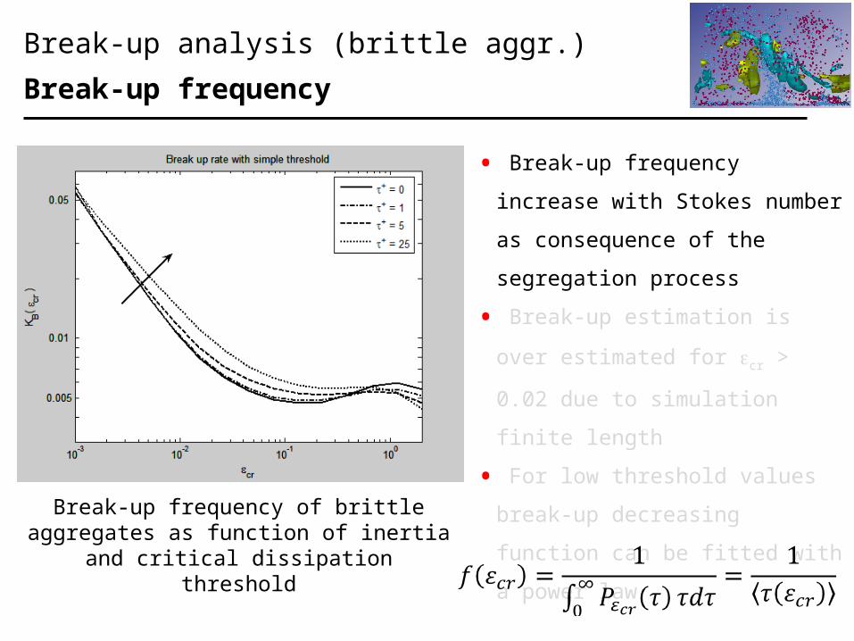
Break-up analysis (brittle aggr.)
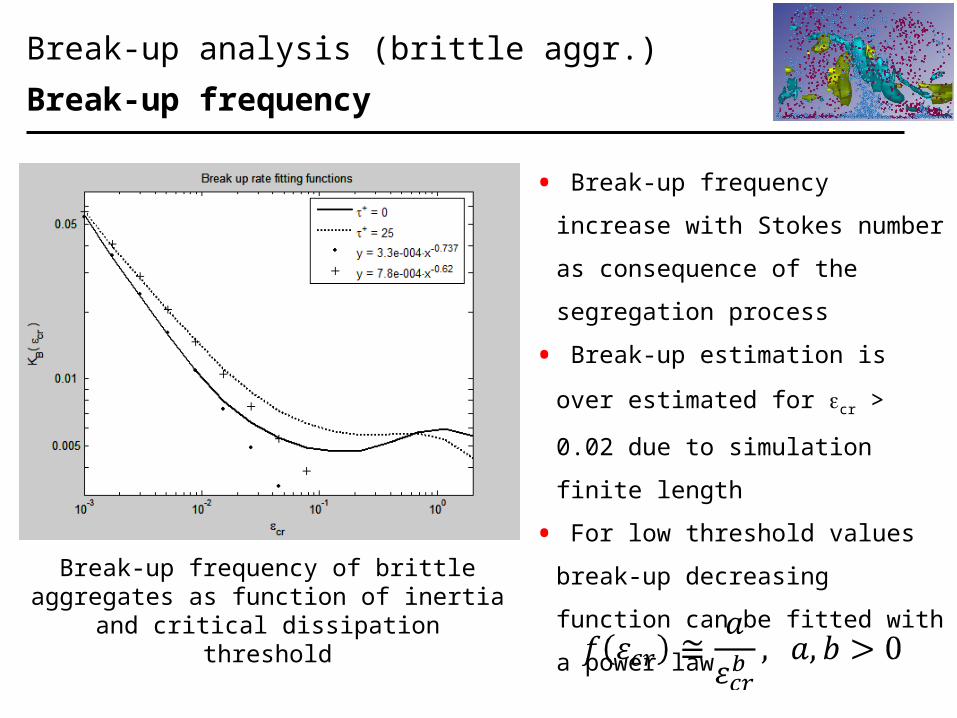
Break-up frequency
Break-up frequency of brittle aggregates as function of inertia and
critical dissipation threshold
• Break-up frequency increase
with Stokes number as
consequence of the segregation
process
• Break-up estimation is over
estimated for ecr > 0.02 due to
simulation finite length
• For low threshold values break-
up decreasing function can be
fitted with a power law
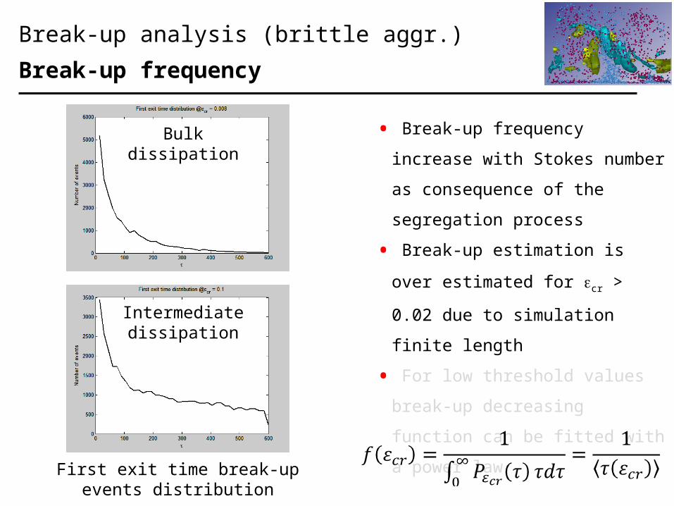
Break-up analysis (brittle aggr.)
Break-up frequency
• Break-up frequency increase
with Stokes number as
consequence of the segregation
process
• Break-up estimation is over
estimated for ecr > 0.02 due to
simulation finite length
• For low threshold values break-
up decreasing function can be
fitted with a power law
First exit time break-up
events distribution
Bulk dissipation
Intermediate dissipation
Break-up analysis (brittle aggr.)
Break-up frequency
Break-up frequency of brittle aggregates as function of inertia and
critical dissipation threshold
• Break-up frequency increase
with Stokes number as
consequence of the segregation
process
• Break-up estimation is over
estimated for ecr > 0.02 due to
simulation finite length
• For low threshold values break-
up decreasing function can be
fitted with a power law
Break-up analysis (deformable aggr.)
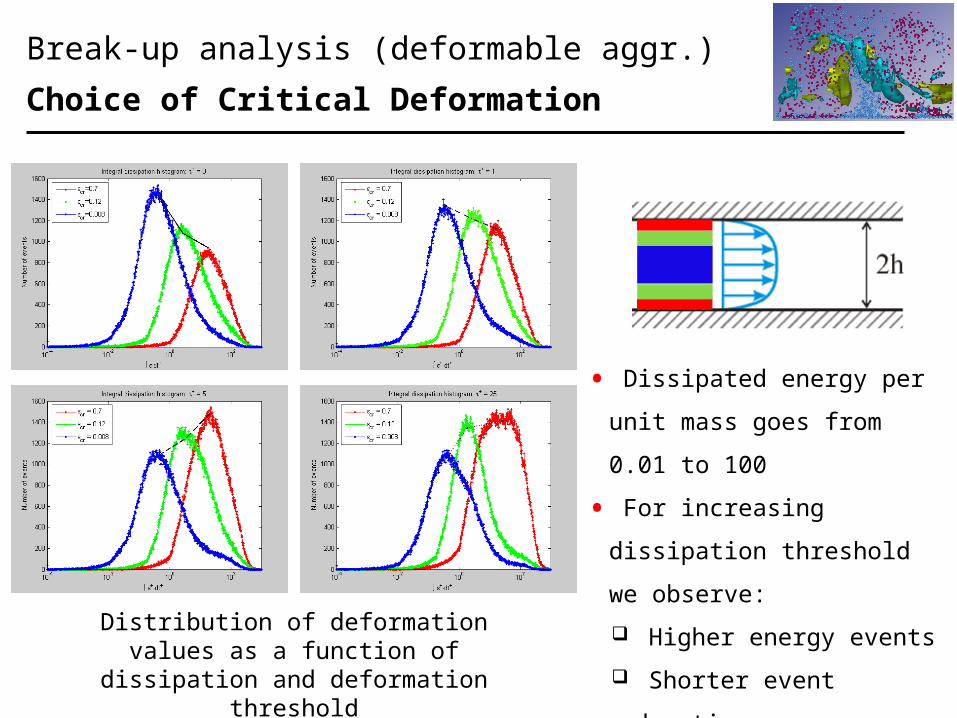
Choice of Critical Deformation
Distribution of deformation values as a function of dissipation and
deformation threshold
• Dissipated energy per unit
mass goes from 0.01 to 100
• For increasing dissipation
threshold we observe:
Higher energy events
Shorter event duration
• Events number depend on
the Stokes number
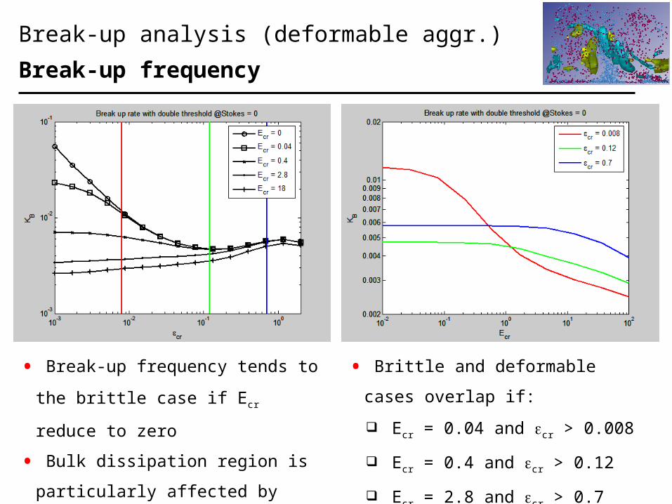
Break-up analysis (deformable aggr.)
Break-up frequency
• Break-up frequency tends to the
brittle case if Ecr reduce to zero
• Bulk dissipation region is
particularly affected by
deformation (red curve on the
right plot)
• Brittle and deformable cases
overlap if:
Ecr = 0.04 and ecr > 0.008
Ecr = 0.4 and ecr > 0.12
Ecr = 2.8 and ecr > 0.7
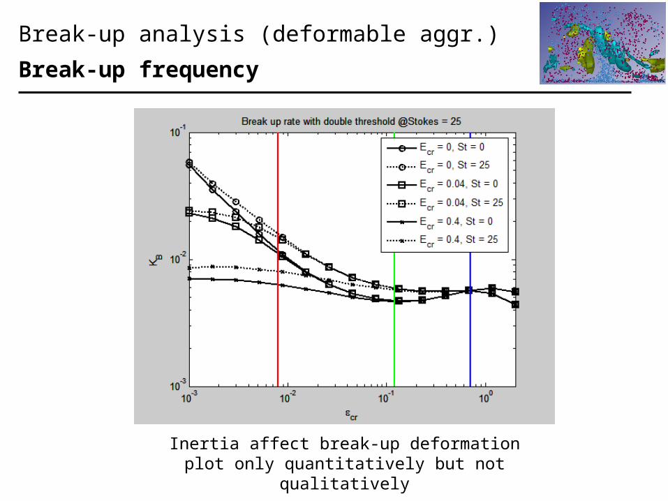
Break-up analysis (deformable aggr.)
Break-up frequency
Inertia affect break-up deformation plot only quantitatively but not qualitatively