PERFORMANCE OF SECTORS EXPORT AND THIER EFFECTS ON

ECONOMIC GROWTH IN ETHIOPIA:

(DISAGGREGATE APPROACH)

Tesfa-Amlak Gizaw(M.sc.)1 and Abebe Habte(Phd)2

1. Economics Department, Dilla University, Dilla Ethiopia (Email: tesfanatan@yahoo.com)

2 Economics Department, Arba Minch University, Arba Minch Ethiopia (Email: aendale@gmail.com)

Abstract

In numerous economic theories; the originators and developers of growth model had

been signified the growth economies altered by different variables. Among these

variables, as to some economist, since export orientation boosts total productivity

through its sympathetic effect on the efficiency of resource allocation, capacity

utilization, economies of scale and technological advancement it determine output growth

in both developing and developed countries. But some other state that the effects of export

varies country to country and items to items depending on the level of development.

Having these and others arguments in mind, the performance as well as the short run and

long run effects of disaggregate export on Ethiopian economic growth mainly designed in

advance. To this end, the 41 years data has been collected from different sources and analyzed

using both descriptive and econometric techniques. The findings of descriptive analysis

reveals that despite of the poor performance which has been recorded in between post

1974/75 and early pre reform period; the performance of agriculture and service exports

have been improved in amid 1992/93 and 2014/15, in particular it is portrayed the

unprecedented service export has been leading the export sector throughout post reform

period. However, that of the industry export in spite of little improvement; its

performance has been poor throughout the study period. Likewise the result of VECM

model reveals; in the long run all sectors’ export absolutely and significantly affect

economic growth but in the short run though their effects are positive their individual

contribution is insignificant the economy. In conclusion albeit it is not encourage-able to say

the short run contribution of each disaggregate export to economic growth is significant, since

their donation is significant in the long run; indispensible measure should be taken to develop

export in general and each disaggregate export in particular.

Key words: disaggregate export, economic growth and VECM model

i

1. INTRODUCTION

Countries’ economic growth influenced by enormous variables, among these variables, as to

many economist because export orientation scale-up total productivity through its

sympathetic effect on the efficiency of resource allocation, capacity utilization, economies of

scale and technological advancement, export affect the growth of economies both in

developing and developed countries.

Albeit export trade highly believed to play critical role in promoting economic growth of

countries, since a number of developing counties import industrial product while they rely on

very few agriculture product exports and also since the income sensitivity of demand for

these products are reasonably lower than imported industrial products, majorities of

developing countries; due to excess import payment over earnings from export, experience

deficit on their current account balance. As a result, according to Todar (2006) the export

potential of a good number of developing countries has been relatively puny compared with

export performance of the developed countries.

This is true when one analyzes about the performance of export and its relation with output

growth in Ethiopia. For the past decades the country merchandise export depended highly on

these three major agricultural products: coffee, oilseed and chat which are basically income

inelastic and have unstable price in the international market. In other word the country has

been exporting large volume of less value merchandise items however, even in recent year,

earned approximately not more than two billion dollars which is below 3.6 billion US dollar

cocoa export revenue in Ivory Coast. Likewise in spite of huge service export potential in

Ethiopia surprisingly the overall service export revenue of the country is not exceeding three

billion US dollar which is also much below more than 9 billion US dollar tourism export

revenue in Egypt. But conversely the country used to import less volume of high value

industrial products and with many development programs; has a plan for importing

intermediate capital goods and hence the trade balance of the country getting deteriorated

time to time.

Loosely speaking Ethiopia’s trade balance has always remained unfavorable and its

unpleasantness has been also increasing significantly, according to Wondaferahu (2013)

1

although Ethiopia’s total exports have been mounting at an average rate of 15.23 percent

during the year 1970/71 to 2010/11 the sector is evidenced by lower export to GDP ratio and

declining share of export in import financing. For instance the exports of goods in Ethiopia

are merely about 7 percent of GDP, compared to an average of near 30 percent of GDP in

sub- Sahara Africa. With regard to share of world export Ethiopia’s share in total world

export despite experiencing linear average increasing trend of about 7% annually from 2000

to 2011 still it is very low, equal to 0.014 % in 2011 Alemayehu (2015).

To address the problems of export sector and strengthen the role of export on output growth,

though a few number of studies exists regarding the effect of export on economic growth in

Ethiopia almost all of them focused merely on the aggregate export and even those who tried

to show at disaggregate level stressed on the impact of a single sector export on output

growth. But this kind of arguments heavily uncovered for major shortcomings of aggregation

and single line arguments. Thus bearing these shortcomings and fill the gap in mind; this is

work undertaken over the effect of disaggregate export on economic growth in Ethiopia.

2. LITERATURE REVIEW

In the late seventeenth century Mercantilism had came up with ``commercial revolution``

which was one of typical explanation of mercantilism thought. And this philosophy of

mercantilism strongly suggests that if a country wants gain from the international trade, it

should promote the export performance and limited import. This would have a positive gain

for the country to scale up production and productivity Thus, according to Mercantilism’s

trade theory thought if country enjoyed a positive trade balance or increase wealth or export

over import. This positive trade balance amass a number of precious metals, gold and silver,

which mean more army, strong navy , expansion of colonies, more raw materials for the

production of export ,low unemployment and better GDP growth. . (Ajami, 2006)

Conversely classical economist argued that increasing specialization and the division of

labor, coupled with international exchange, would contribute to raise welfare and growth of a

nation. It can be deduced that Smith saw international trade as a welfare-enhancing

mechanism: the division of labor required people exchanging goods and services. Higher

levels of trade would imply more specialization – division of labor- and by these means,

2

economic growth would be enhanced. And also David Ricardo’s two countries-two goods-

one factor of production example proposes gains from trade and specialization for the

countries involved, even when one of the countries is more efficient in the production of both

goods. That is pattern of trade, being determined by comparative advantage, increases

welfare in both nations by means of improvements in production and consumption

efficiency. (Van den and Lewer, 2007).

Similarly the standard Heckscher-Ohlin model proposes that trade enhances welfare for the

nations engaged in trade, considering that countries realize higher levels of aggregated utility

as compared to autarky. Aggregate welfare gains from free trade are classified into two

distinct effects; namely, production efficiency gains and consumption efficiency gains And

based on, general equilibrium model with one single factor of production (labor) and

economies of scale internal to the firm, imperfect competition assuming n different goods

and consumers’ taste for variety- the so-called New Trade Theory shows trade as beneficial,

since it increases market size (Krugman and Obstfeld, 2006).

(Balassa, 1978) it argued that in a usual production function framework, capital and labors

are the main determinants of economic growth. However, this neglects the fact that 'export

orientation raises total productivity through its favorable effect on the efficiency of resource

allocation, capacity utilization, economies of scale and technological change and hence the

need to include export within this production-type framework. The study found that the 'rate

of growth of exports importantly affected the rate of economic growth.

Begum and Shamsuddin (1998), investigate the impact of exports on economic growth for

the period 1961-92 using a two sector growth model. The key finding of their study is that

export growth has significantly increased economic growth of the country through its

positive impact on total factor productivity.

Sanjuan-Lopez and Dawson (2010) estimated the contribution of agricultural exports to

economic growth in developing countries. They estimated the relationship between Gross

Domestic Product and agrarian and non agrarian exports. The results of the study indicated

that there existed long run relationship and the agriculture export elasticity of GDP was 0.07.

The non agriculture export elasticity of GDP was 0.13.Based on the empirical results, the

3

study suggested that the poor countries should adopt balanced export promotion policies but

the rich countries might attain high economic growth from non agricultural exports.

Ugwuegbe S. And Uruakpa (2013) examined the impact of disaggregate export on economic

growth in Nigeria, by employing annual time series data from 1986-2011. The result reviles

that both oil and non oil export positively and significantly affect economic growth in

Nigeria.

Gilber, Linyong and Divine (2013) explore the contribution of agricultural exports to

economic growth in Cameroon for the period 1975-2009. Coffee export and banana export

has a positive and significant relationship with economic growth. On the other hand, cocoa

export was found to have a negative and insignificant effect on economic growth.

Ijirshar (2015) investigate the impact of agriculture exports on economic growth in Nigeria

using error correction model and consisting annual data for the period 1970-2012. The key

finding of their study is that agriculture export growth has positively contributed to economic

growth of the country through its positive impact on total factor productivity

4

3. RESEARCH METHODOLOGY

3.1. Type and Source of Data

This study considered 41 years time series secondary data. The main source of these data are

National Bank of Ethiopia (NBE), Ethiopia Revenue and Custom Authority (ERCA), Central

Statistics of Authority (CSA), Ministry Finance and Economic development (MoFED) and

World Bank (WB) countries development indicators Data base.

3.2. Methods of Data Analysis

The analytical framework of this work consist both descriptive and empirical ingredient. In

the descriptive analysis part the trends of real GDP and the performances of disaggregate

exports analyzed through employing some descriptive statistical analysis methods, in

particular measures of location employed. In the econometrics section, multivariate

regressions analysis of co-integration VAR model has been employed. This is because the

co-integrated VAR model has gained reputation in recent empirical research for a number of

reasons for instance (i) the effortlessness and relevance in analyzing time-series data, and (ii)

the ability to guarantee stationarity and to make available the extra channels through which

both the short run and long run effect could be detected when two variables are co-integrated.

3.3. Model specification

To examine the effect of export on economic growth some theoretical models considered in

this study. First the neoclassical growth model with two factor production functions, capital

and labor as determinants of output imitated as follows.

Y = Af (K, L) ------------------------------------------------------------------------------------------ (1)

Where Y is aggregate real output, K and L represent capital and labor, respectively and A is

exogenously determined level of technology.

The second theoretical base which considered in this work is the neo-classical growth model

which modified and suggested by (Balassa, 1978) as follow.

Y = A f (L, K, X) -------------------------------------------------------------------------------------- (2)

5

Where Y is aggregate real output, K and L represent capital, labor and export respectively.

Finally, the model that used in this study is the adopted Ugwuegbe and Uruakpa (2013)

imperfect substitution model which is expressed as follows:

RGDPt = f (RAEXPt, RIEXPt, RSEXPt,RIMPt, IRt, dummy)---------------------------------(3)

And equation 7 log-linear-zeds as follow:

LRGDPt= β0+ β1LRAEXPt+ β2LRIEXPt+ β3LRSEXPt+ β4LRIMPt + β5LCPIt + β6dummy + et-----------(4)

Where, LRGDP = Real GDP at time t in log form is the dependent variable.

LRAEXP = Real Agricultural Export at time t in log form is independent variable

LRIEXP = Real industry Export at time t in log form is independent variable

LRSEXP = Real Service Export at time t in log form is independent variable

LRIMP = Real import of goods and service at time t in log form is independent variable

LIR = inflation rate at time t is independent variable

Dummy = proxy variable for political stability

β0 is intercept parameter

β1, β2, β3, β4, β5, β6 are slope parameters

et is error term

3.4. Estimation Technique

The major econometric techniques which employed in this research are; stationarity test, co-

integration test and diagnosis tests

3.4.1. Stationary test

Stationarity in time-series data refers to a stochastic time series that has three characteristics,

as described. First, a variable over time has a constant mean. Second, the variance of a

6

variable over time is constant. Third, the covariance between any two time periods is

correlated. If one or more of these criteria is violated, then the data generating process of the

time-series data is a non-stationary series (Gujarati, 1995).

A series may be difference or trend stationary. A difference stationary series becomes

stationary after successive differencing while a trend stationary series becomes stationary

after deducting an estimated constant and a trend from it. There are many tests for examining

the existence of unit root problem. As the error term is unlikely to be white noise, Dickey and

Fuller have extended their testing procedure suggesting an augmented version of the test that

incorporates additional lagged term of dependent variable in order to solve the

autocorrelation problem.

If the series is non stationary at level form, then, the test is carried out successively on the

differenced series until it becomes stationary. The order of integration is then established.

The test has variants as below:

-With drift and trend

-With drift and no trend and

Δ y t=δ0+δ 1 y t−1+∑i=1

p

θi Δ y t−i+εt

-------------- (5)

Δ y t=δ1 y t−1+∑i=1

pθi Δ y t−1+εt

------------- (6)

Where, δ0 and t are the constant and the time trend, respectively. The ADF test assumes that

the errors are statistically independent and have a constant variance. Thus, an error term

should be uncorrelated with the others, and has a constant variance. The test is first carried

out with a constant and trend on the variable in level form. Secondly, it is carried out with a

constant only and finally without constant or trend, on the differenced variable depending on

which was significant in the level form. Then

- If the ADF test statistic is greater than the critical value, then the series is stationary.

7

- If the ADF statistic is less than the critical value, the series is non-stationary.

3.4.2. Optimal Lag Specification

There are two approaches for the determination of optimal lag length: Cross-equation

restrictions and Information criteria. Cross-equation restrictions deal either about general to

specific procedure or vice versa to determine the optimal lag length. This means estimating

the VAR model for a maximum number of lags, then reducing down by re-estimating the

model for one lag less until it reaches zero lag.

Alternatively information criterion focus choosing the lag length that minimizes the value of

the information criteria such as (LR), the Final Prediction Error (FPE), the Akaiki

Information Criterion (AIC), the Schwarz Information Criterion (SIC), and the Hannan

Quinn Information Criterion (HQ) are appropriate for the examination of finite lag order

VAR model. Usually, the model with the smallest, AIC or SIC values are preferred.

3.4.3. Co-integration Test

Co integration is the statistical implication of the existence of long run relationship between

the variables which are individually non-stationary at their level form but stationary after

difference (Gujarati, 1995)). The theory of co-integration can therefore be used to study

series that are non stationary but a linear combination of which is stationary. Two main

procedures can be used to test for co-integration: The Engle and Granger (1987) test and the

Johansen (1988) co-integration test. Johansen procedure of co integration gives two statistics.

These are the value of LR test based on the maximum Eigen – value and on the trace value of

the stochastic matrix. The Johansen test uses the likelihood ratio to test for co-integration.

The decision rule compares the likelihood ratio to the critical value for a hypothesized

number of co-integrating relationships. If the likelihood ratio is greater than the critical value,

the hypothesis of co-integration is accepted. Alternatively the Engle and Granger test is a two

step test which first requires that the variables be integrated of the same order. The first step

consists of estimating the equation in level form, while the second step consists of testing the

stationarity of the residuals, of the estimated equation. The existence of co integration is

confirmed if the residuals are stationary at level form.

When we have more than one endogenous variable, no longer need to talk of ECM but

8

VECM. The Vector error correction model follows the observation by (Engel and Granger,

1987) that a group of co-integrated variables can be expressed as a Vector error correction

model in which all the variables are stationary at I(1). This model can be estimated using the

ordinary least squares procedure without risk of spurious correlation. Also, the coefficient of

the lagged residual of the long-run co-integrating equation referred to as the error correction

term can be used as evidence of the existence of a short-run relationship between the

variables. A negative error correction coefficient provides ample evidence of the existence of

a long-run relationship. The size of the error correction coefficient determines the speed of

adjustment towards equilibrium.

In this study, the VECM estimated as follows;

∆LRGDPt= β0 + β1∆LRAEXPt+ β2∆LRIEXPt+ β3∆LRSEXPt+ Β4∆LRIMPt+ αεt-1------------------------- (13)

Where, ∆L represents the change in natural logarithm of the variable, for example

∆LRGDPt is the change in natural logarithm of real gross domestic product β0 is the

constant term, β1, β2, β3 and β4 parameters of the independent variables and εt stochastic error

term εt-1, lag of the residual term representing short run disequilibrium adjustments of the

estimates of the long run equilibrium error, α is the coefficient of the error correction term.

And the alternative hypothesis of the existence of a long-run relationship between the

dependent and the independent variables, defined;

H0: β1= β2 = β3 = 0

As against H1: β1= β2 = β3 ≠ 0

The decision rule is that if the p-value is less than the chosen α with 5% level of

significance, we accept H1, meaning the coefficients of the dependent variables are

statistically significant and different from zero. But if the p-value is greater than the chosen,

we reject H1, meaning the coefficients of the dependent variables are statistically insignificant

and equal to zero

9

0

100

200,

300

400

500

1975 1980 1985 1990 1995 2000 2005 2010 2015

RAEXP RIEXP RSEXP

4. RESULT AND DISCUSSION

4.1. Descriptive Result and Discussion

Disaggregate export performance analysis

As you can see from figure 2 below, agriculture export throughout the study period

significantly surpassed industrial export and dominated the merchandise export. In 1974/75

in absolute term the real value of agriculture export was 57.76 mill ETB and this number

reached to 289.9 mill ETB in 2014/15 with an average growth rate of 10.8 percent between

1974/75 and 2014/15. More specifically from 1974/75 to 1983/84 real value of agricultural

export grew by 2.26 percent and then went-down by 16.97 percent on average from 1984/85

to 1991/1992 and soon after the reform program recovery on the real earning agriculture

export witnessed and hence from 1992/93 to 2015 real revenue from agriculture export grew

by 23.82 percent on average.

Figure 1: Trends of disaggregate export during 1974/75 to 2014/15 (in millions birr)

Source: Own calculation based on various year NBE, ERCA and World Bank data

10

Regarding industry and service export figure 2 also clearly show except some years, the

improvement in the real value of the two exports observed during the study period. Despite

fluctuation exist between maximum real value of 65.32 million ETB and 418.4 million ETB

in 2010/11 and minimum real value of 1.05 million and 16.45 million ETB in 1978 FY in the

two exports, from 1974/75 to 20/4/15 real earning of industrial and service Export grew by

16.14 and 12.59 percent respectively on average (See figure 2).

-80

-40

0

40

80

120

160

200

240

280

1975 1980 1985 1990 1995 2000 2005 2010 2015

% Change RAEXP% Change RIEXP% Change RSEXP

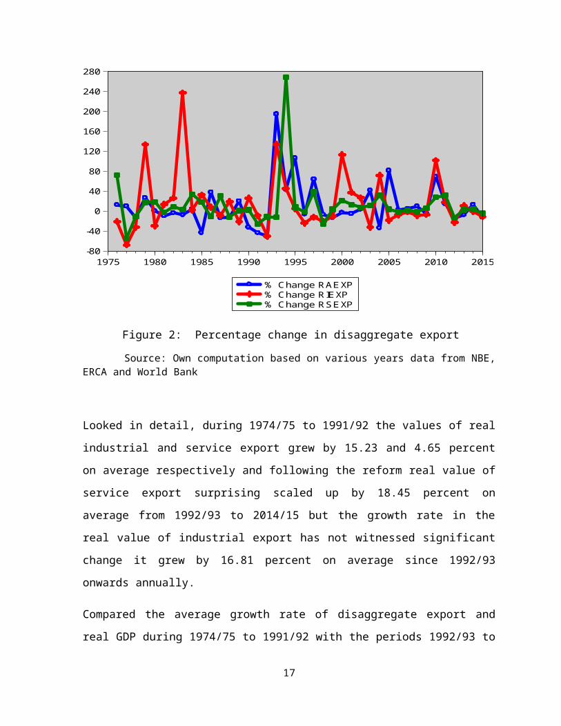
Figure 2: Percentage change in disaggregate export

Source: Own computation based on various years data from NBE, ERCA and World Bank

Looked in detail, during 1974/75 to 1991/92 the values of real industrial and service export

grew by 15.23 and 4.65 percent on average respectively and following the reform real value

of service export surprising scaled up by 18.45 percent on average from 1992/93 to 2014/15

but the growth rate in the real value of industrial export has not witnessed significant change

it grew by 16.81 percent on average since 1992/93 onwards annually.

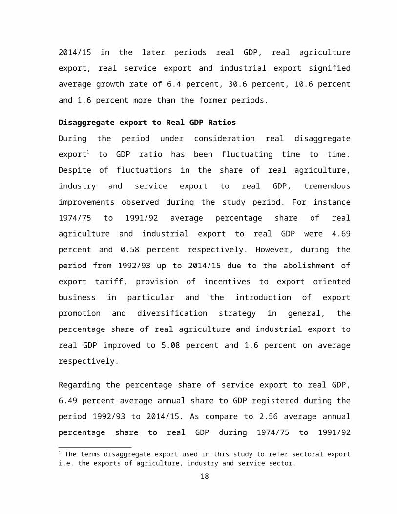
Compared the average growth rate of disaggregate export and real GDP during 1974/75 to

1991/92 with the periods 1992/93 to 2014/15 in the later periods real GDP, real agriculture

11

export, real service export and industrial export signified average growth rate of 6.4 percent,

30.6 percent, 10.6 percent and 1.6 percent more than the former periods.

Disaggregate export to Real GDP Ratios

During the period under consideration real disaggregate export1 to GDP ratio has been

fluctuating time to time. Despite of fluctuations in the share of real agriculture, industry and

service export to real GDP, tremendous improvements observed during the study period. For

instance 1974/75 to 1991/92 average percentage share of real agriculture and industrial

export to real GDP were 4.69 percent and 0.58 percent respectively. However, during the

period from 1992/93 up to 2014/15 due to the abolishment of export tariff, provision of

incentives to export oriented business in particular and the introduction of export promotion

and diversification strategy in general, the percentage share of real agriculture and industrial

export to real GDP improved to 5.08 percent and 1.6 percent on average respectively.

Regarding the percentage share of service export to real GDP, 6.49 percent average annual

share to GDP registered during the period 1992/93 to 2014/15. As compare to 2.56 average

annual percentage share to real GDP during 1974/75 to 1991/92 significant improvement also

observed in the percentage share of real service export to real GDP. In general from 1974/75

to 2014/15 on average real agriculture, industry and service export accounts for 5 percent,

0.85 percent and 4.76 percent of GDP respectively.

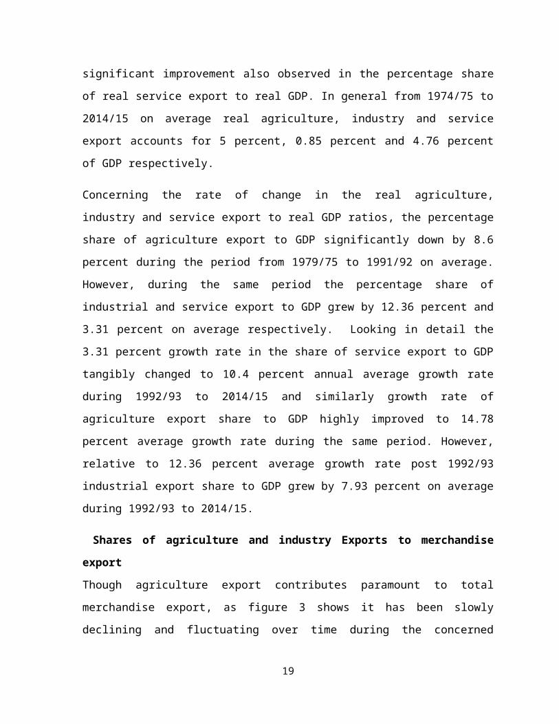
Concerning the rate of change in the real agriculture, industry and service export to real GDP

ratios, the percentage share of agriculture export to GDP significantly down by 8.6 percent

during the period from 1979/75 to 1991/92 on average. However, during the same period the

percentage share of industrial and service export to GDP grew by 12.36 percent and 3.31

percent on average respectively. Looking in detail the 3.31 percent growth rate in the share

of service export to GDP tangibly changed to 10.4 percent annual average growth rate during

1992/93 to 2014/15 and similarly growth rate of agriculture export share to GDP highly

improved to 14.78 percent average growth rate during the same period. However, relative to

12.36 percent average growth rate post 1992/93 industrial export share to GDP grew by 7.93

percent on average during 1992/93 to 2014/15.

1 The terms disaggregate export used in this study to refer sectoral export i.e. the exports of agriculture, industry and service sector.

12

0

20

40

60

80

100

1975 1980 1985 1990 1995 2000 2005 2010 2015

RAXTRMDEXP RIXTRMDEXP

Shares of agriculture and industry Exports to merchandise export

Though agriculture export contributes paramount to total merchandise export, as figure 3

shows it has been slowly declining and fluctuating over time during the concerned period.

From 1974/75 up to 1983/84 on average the share of agriculture export to merchandize

export was 94.6 percent, it went down to 73.5 percent during 1984/85-1991/92. After while

its share reversed and scaled-up to 81.1 percent on average during 1991/92-2014/15.

Whereas the share of industry export to merchandise export had been small and largely

depends up on the share of agriculture export, but except in some years its share has been

improving 1984/85 on ward. For instance from 1974/75 to 1984/85 the share of industrial

export to total merchandise export was 5.4 percent on average however during 1984/85 to

2014/15 tremendously improved to 20.3 percent on average, showing 275.93 per cent growth

rate.

Figure 3: Percentage share of agriculture and industry export to merchandise export

Figure 4 on the other hand shows from 1974/75 to 2014/15 the share of agriculture export to

total merchandise export with ups and downs dominated and controlled merchandise export

13

with 83.3 percent average share and industrial export distantly go after with 16.7 percent

average share slowly behind the share of agriculture export.

RAXTRMDEXP RIXTRMDEXP

Means

83.3 %

16.7 %

Figure 4: average shares of agriculture and industry export to merchandise export from 1974/75-2014/15

Source: Own calculation based on various year data from NBE and ERCA

Shares of agriculture, Industry and service export to total goods and service export

As indicated in figure 5 the share of agriculture export to aggregate goods and service export

fluctuate between 78 percent and 21 percent. From 1974/75 to 1991/92 the average

contribution of agriculture export to aggregate export was 57.12 percent but during the same

period its average share went down by 5.1 percent annually. Nonetheless, in spite of 6.1

percent average growth from19992/93 to 2014/15 agriculture contributes 40 percent to

aggregate export on average.

14

0

10

20

30

40

50

60

70

80

1975 1980 1985 1990 1995 2000 2005 2010 2015

RAXTRGSX RIXTGSX RSXTRGSX

Figure 5: % shares of agriculture, industry and service export to aggregate export

Source: Own calculation based on various years data from NBE, ERCA and World Bank

As to the share of service and industry export to the aggregate export, their share fluctuate

between minimum values of 19 percent and 7 percent and maximum values of 65 percent and

21 percent respectively during the study period. More specifically, their share were 27

percent and 7 percent respectively in 1974/75, it reached to 65 percent in 1991/92 and 21

percent in 1992/93 respectively and at the end of 2014/15 moved back to 52 percent and 7

percent respectively.

15

-80

-40

0

40

80

120

160

200

240

1975 1980 1985 1990 1995 2000 2005 2010 2015

% Change RAXTRGSX% Change RIXTGSX% Change RSXTRGSX

Figure 6: growth rate of agriculture, service and industry export share to aggregate export

Source: Own calculation of data from NBE, ERCA and World Bank data

Figure 8 shows, from 1974/75-1991/92, the contribution of service export to aggregate export

and its share growth rate averaged at 34.7 percent and 7.6 percent respectively. However,

from the period 1991/92 to 2014/15 even though the growth rate of service export share on

average grew by 0.57 percent, its contribution to aggregate export improved to 51.05 percent

and with this share it dominated the aggregate export by turning the dominance of agriculture

export share down below it for the past 33 years from 2014/15. Similarly from 1974/75 to

1991/92 the share of industry export to aggregate export and its growth rate averaged at 8.2

percent and 17.7 percent consecutively. And then with little improvement during 1992/93 up

16

to 2014/15 the share of industry export to aggregate export on average scaled-up to 8.8

percent but its share growth rate average at 1.5 percent.

RAXTRGSX RIXTGSX RSXTRGSX

Means

47.6 %

43.8 %

8.6 %

Figure 7: Average share of agriculture, industry and service export to aggregate export

from1974/75-2014/15.

Source: Own calculation of data from NBE, ERCA and World Bank data

And figure 7 portrays a bulk of export, on average 47.6 percents and 43.8 percent out of the

aggregate export contributed by agriculture and service export while industry export share

the remaining insignificant 8.6 percent during the study periods.

17

4.2. Econometrics Results and Discussion Results of Stationarity Test.

Like most macroeconomic series the results of the unit root test of all variables except LCPI

are not stationary at their levels and become stationary at their first difference.

Table 4.1: Augmented Dickey-Fuller (ADF) stationarity test results

ADF test statistics

Variable

s

Intercept

Critical

Intercept Critical

prob.

Remark

s

No trend value And

trend

value

LRGDP -2.020151 -3.621023 -6.635440 -4.219126

0.0000

I(1)

LRAEXP -6.540730 -3.610453 -6.549601 -4.211868

0.0000

I(1)

LRIEXP -6.240128 -3.610453 -6.151209 -4.211868

0.0000

I(1)

LRSEXP -7.381334 -3.610453 -7.390909 -4.211868

0.0000

I(1)

LRIMP -8.285444 -3.610453 -8.451934 -4.211868

0.0000

I(1)

Notes: A variable is stationary when ADF test statistics are greater than the CV at a

given level.

Source: E-views version 7 outputs

As we can see from Tables 4.1 the stationarity test for all variables, at their first differences,

strongly reject the unit root which mean they are an integrated of order of one, meaning they

are stationary.

Co-integration Test Result

18

The employed Johansen test result that is both tests; the maximum eigen value and trace

statistics indicates the existence of one co-integrating relationship (see table 4.3 and 4.4)

Table 4.3: Johansen co-integration tests (Trace)

List of variables included: LRGDP, LRAEXP, LRIEXP, LRSEXP, LRIMP

Null

hypothesis

Alternative

hypothesis

Eigen value Trace

statistic

Critical

Value(5%)

Prob.**

r=0* r≥0  0.832604  88.08627  69.81889  0.0009r≤1 r≥1  0.383785  29.10237  47.85613  0.7635r≤2 r≥2  0.200912  13.12510  29.79707  0.8858r≤3 r≥3  0.128374  5.723726  15.49471  0.7279r≤4 r≥4  0.035409  1.189702  3.841466  0.2754

Source: E-views 7 output.

Trace test indicates 1 co-integration equation(s) at the 0.05 level, * denotes rejection of the

hypothesis at the 0.05 level, **MacKinnon-Haug-Michelis (1999) p-values and r denotes the

rank of long run matrix

Table 4.4: Johansen co-integration tests (Max-Eigen)

Null

hypothesis

Alternative

hypothesis

Eigen

value

Max-

Eigen

statistic

Critical

value

(5%)

Prob.**

r=0* r=1  0.832604  58.98389  33.87687  0.0000r=1 r=2  0.383785  15.97728  27.58434  0.6678r=2 r=3  0.200912  7.401369  21.13162  0.9364r=3 r=4  0.128374  4.534025  14.26460  0.7991r=4 r=5  0.035409  1.189702  3.841466  0.2754

19

Source: E-views 7 output. Max-Eigen test indicates 1 co-integration equation(s) at the 0.05

level, * denotes rejection of the hypothesis at the 0.05 level, **MacKinnon-Haug-Michelis

(1999) p-values and r denotes the rank of long run matrix

Both of the above tables show the null hypothesis claims no co-integration is rejected at the

conventional level of significance. This is because both the trace test statistic and Max-Eigen

statistic greater than the critical values at zero co-integrating vector in their respective tests,

which means the null hypothesis of no co-integration(r=0) among the variables is rejected at

the 5% level of significance. And hence these results demonstrate that the considered

variables are co-integrated so that it ensure the presence of long run equilibrium relationship

among them and additionally it may reveals the existence of causation between endogenous

and exogenous variables at least in one direction.

Vector Error Correction Model (VECM)

Once the modeled variables co-integrated, in the next step vector error correction model

(VECM) which combined both the long run properties and short run dynamics has been

estimated. And the results of long run and short run models presented as follows.

Long Run Model Results

The result of long run model reveals that all the variables have the anticipated signs and are

of reasonable magnitude. In other word all explanatory variables except import ride the same

horse with dependent variable; loosely speaking agriculture export, industry export and

service export positively affect economic growth while import is negatively related with

output growth

The estimated long run model with t-statistics in the parenthesis stated as:

LRGDP = 6.916942 + 3.398395LRAEXP + 1.064308LRIEXP + 1.743059LRSEXP-7.136312LRIMP

(7.60580) (2.66963) (2.55869) (-11.5886)

In the long run holding other variables remains constant, the finding reveals that

agriculture export has a positive and significant relationship with economic growth

in Ethiopia. That is, a one percent increase in agriculture export stimulates economic

growth by 3.4 percent in Ethiopia. This because agriculture export is principal factor

20

in guaranteeing equilibrium in the balance of payments and, as a consequence,

guaranteeing macroeconomic stability and economic growth of developing

countries. And hence this result is consistent with the findings of (Usman and Mc

millan, 1998; Gilbert, 2009; Sanjuan lope and Dawson, 2010).

Similarly service export positively and significantly related with output growth in

Ethiopia. That is a 1% increase in service export leads to a 1.7 percent rise in

economic growth in Ethiopia in the long run. This is because exporting service

motivates the economies of developing countries through generating foreign

currencies, creating jobs and financing their trade deficit. Thus this finding is line

with Ziramba (2011), Rashid Mohamed, Yee Liew and Said S. (2012) among other.

Even though the effect of industry export is small, it affects economic growth

positively and significantly. That is a 1% increase in industry export, in the long run,

leads to a 1.1 percent increase in economic growth in Ethiopia. Such findings can be

interpreted as stemming from the effects of increased productivity associated with

the industrial sector compared to those depending on primary goods. Thus this

finding is accordance with the findings of Greenaway, D. Morgan and Wright (1999)

and Herter (2004 and 2006).

Results of Short Run model

From the short run model result we can observe that error correction term (ECM-1)) is

negative as expected but insignificant and the coefficients of all independent variables except

import and dummy variables are insignificant at 5%. Besides table 4.5 reveals the value of

error correction term ECM (-1) is -0.88% signifying a very low speed of adjustment that is

the speed at which a deviation from long equilibrium is removed slowly where 0.88% of

disequilibrium adjusted in each year. Which means the full disequilibrium will be adjusted

approximately after 100 years.

From the result below the short run effects of agriculture and industry export on economic

growth in Ethiopia are positive but insignificant. That is a 1% increase in agriculture and

industry export leads to a 0.032 percent and 0.013 percent increase in economic growth. Thus

these results suggest that in the short-run the two exports are insignificant in affecting

21

economic growth in Ethiopia. Similarly, the short run effect of service export on the

economic growth is positive but insignificant. That is a 1% increase in service export leads to

a 0.014 percent increase in economic growth. These kinds of export effect on output growth

are quite realistic when the growth paths of the two time series are determined by other,

unrelated variables (for example, investment) in the economic system (Pack, 1988)

Table 4.5: Estimates of short run Parameters

Dependent variable: DLRGDP

Variables CoefficientCoefficient Std. ErrStd. Err t. statistict. statistic Prob.

DLRAEXP(-1) 0.031778 0.026133 1.216019 0.2353

DLRIEXP(-1) 0.013544 0.020270 0.668166

0.5102

DLRSEXP(-1) 0.014081 0.028225 0.498881 0.6222

DLRIMP(-1) -0.104304 0.047418 -2.199681

0.0373*

C 0.045206 0.022836 1.979530 0.0589

DUMMY 0.076961 0.018193 4.230188 0.0003*

ECM(-1) -0.008811 0.007030 -1.253402 0.2217

R-squared 0.632330     Mean dependent var

S.D. dependent var

 Akaike info criterion

    Schwarz criterion

0.051372

Adjusted squared 0.529382 0.058471

S.E. of regression 0.040112 -3.387066

Sum squared

resid

0.040224 -3.024277

22

    Hannan-Quinn criter.

    Durbin-Watson stat

Log likelihood 63.88659 -3.264999

F-statistic 6.142251 2.019944

Prob(F-statistic) 0.000302

Source: calculation by author using Eviews 7

Note: * indicates significance at 5% level

5. CONCLUSION AND IMPLICATIONConclusionsTo accomplish the objectives of this work both descriptive and econometric methods of

analysis has been used. The findings of descriptive analysis revealed during the study periods

agriculture, industry and service exports have been shared 5 percent, 0.85 percent and 4.76

percent to GDP respectively. In the second performance indicator the trends in growth rates

of values of agriculture, industry and export showed a positive but fluctuation trend with

annual average growth rates of 10.8 percent, 16.14 percent and 12.59 percent respectively.

These rates of growth in the values of disaggregate exports of the country are by far better

during post 1992/93 than average growth rates recorded pre reform periods. A closer look at

the third and fourth indicators agriculture and industry export have been contributed 83.3

percent and16.7 percent to merchandise export and agriculture, industry and service exports

have been shared 47.6 percent, 8.6 percent and 43.8 percent on average to aggregate export

respectively during the study period. And the findings of empirical analysis reveals that in

the long run agriculture, industry and service exports positively and significantly affect

economic growth however, in the short run despite the effect of each disaggregate export on

output growth is positive but their respective contribution is insignificant. In sum despite the

performances of agriculture, industry and service exports have been improving time to time

the short run effects of each disaggregate export on the economic growth is very weak in

Ethiopia. More specifically the performance of industry export, even as viewed from the

angle of service and agriculture export contribution, its contribution to GDP is very tiny. In

general since the world demand for primary agriculture products is not very dynamic,

Ethiopia will not be competitive through merely exporting limited primary products. And

23

hence to realized outstanding performance in the export sector; sustainably standardizing,

diversifying as well as boosting production and productivity of sectors’ output and

implementing sector wise balanced economic development policies and strategies are more

than anything else.

REFERENCE

Ajami R. (2006), ``International business theory and practice`` New York, M:E Sharps USA.

Alemayehu S. (2015), “Ethiopia's External Trade Performance in the Recent Past” Paper submitted at

the 13th International Conference on the Ethiopian Economy.

Balassa, B.(1978), “Exports and Economic Growth: Further Evidence”; Journal of Development

Economics 5: 181-189.

Balassa, B.(1985), “Exports, Policy Choices and Economic Growth in Developing Countries after

the 1973 Oil Shock”; Journal of Development Economics 18: 23-35.

Begum, Shamshad and Abdul F. M. Shamsuddin (1998) “Exports and Economic Growth in

Bangladesh.” The Journal of Development Studies. Vol. 35, No. 1, October 1998. pp. 89-114.

Bhagwati, J., 1988. “Export-promoting trade strategies: Issues and evidence”. The World Bank

Research Observer, 3(1): 25–57.

Dickey, D. and Fuller W. (1981), “Likelihood ratio statistics for autoregressive time series with a

unit root”.Econometrica, No.49, pp.1057 - 1072.

Engel,R.F. and C.W.J. Granger. (1987), “Co-integration and Error Correction: Representation,

Estimation and Testing”; Econometrica 55(2):251-276.

“On Exports and Economic Growth”; Journal of Development Economics 12:59-73.

24

Fernando, U.F.N. (1988), “The Relationship between Exports and Economic Growth in Sri Lanka:

an Empirical Investigation”, Central Bank Staff Studies, Vol.18, No. 1 & 2. pp. 97-126.

Gilber, Linyong and Divine (2013) “The Impact of Agriculture Export on Economic Growth In

Cameroon”. International Journal of Business and Management Review. Vol. 1, No.1, pp

Gujarati, D. (1995), “Basic Econometrics”, 3rd Edition, New York: McGraw-Hill

2166-4951.

Herzer, D (2004): “Export-Led Growth in Chile: Assessing the Role of Export Composition in

Productivity Growth”, Ibero America Institute for Economic Research (IAI) Discussion Papers No

103

Herzer, D. and Nowak-Lehmann D., (2006), “What Does Export Diversification Do for Growth?

An Econometric Analysis”, Applied Economics 38: 1825-1838.

Development organization, Discussion Paper. E-mail: ipr-Publications@unido.org

Johansen, S. (1988), “Statistical analysis of cointegration vectors”. Journal of Economic

Dynamics andControl, No.12, 231 - 254.

Johansen, S. and Juselius, K. (1990). “Maximum likelihood estimation and inference on

Cointegration withapplication to the demand for money”. Oxford Bulletin of Economic

and Statistics, No.52, pp. 169 - 210.

Krugman Paul R., and Obstfeld Maurice, (2006). “Applied time-series econometrics”.

Cambridge: Cambridge University Press.

Mohamed, Yee Liew and Mzee (2012) “Export Trade and Economic Growth in Tanzania”.

Journal of Economics and Sustainable Development. Vol.3, No.12.

NBE (2010), “National Bank of Ethiopia Annual Report, Addis Ababe”.Pack, H., 1988.

“Industrialization and trade”. Amsterdam: Elsevier.

25

Sanjuan-Lopez, A.I. and Dawson, P.J. (2010), “Agricultural exports and economic growth in

developingcountries: A panel co-integration approach”. Journal of Agricultural Economics,

61(3), 565 - 583.

Todaro, M.P. and Smith, S.C., 2006. “Economic development”. London: Pearson-Addison

Weasley.

Ugwuegbe and Uruakpa(2013) , “The Impact of Export Trade on Economic Growth In Nigeria”.

International Journal of Economics, Business and Finance. Vol. 1 PP: 327-341

Vander Berg and Lewer (2007), "International Trade and Economic Growth". Nework: Periss

Press.

Wondaferaw(2013), “Determinant of Export Performance in Ethiopia”. National Monthly

Refereed Journal of Economics and Management. Vol No.2, Issue No.5 ISSN 2277-1166.

World Bank (2012). “www.ethiopiainvestor.com-ethiopia-economic”.

Ziramba, E. (2011), “Export-Led Growth in South Africa: Evidence from the Components of

Exports”, Journal for Studies in Economics and Econometrics, 35 (1): 1-13

26