Embed Size (px)
Citation preview

CHAPTER 1
BACKGROUND
1.0 Introduction
Over the last 100 years the energy consumption in the world has risen exponentially.
Some studies predict that by the middle of this century there will be a rise in the world's
energy consumption by a factor of 4. To supply this huge amount of energy
economically, safely and without polluting the environment will be extremely difficult.
Due to the limitations on conventional sources of energy, few of the current technologies
for power production will outlast the 21st century. Even today, renewable energy offers
the possibility of covering our energy requirement without relying on fossil fuels. An
energy industry could be structured completely on the basis of renewable energies (solar,
wind, geo-thermal, etc.).
The sun represents by far the largest available energy source. From the sun an energy
quantity of 3.9*10^24 J = 1.08*10^18 kWh arrives on the earth's surface every year.
This corresponds to about 10,000 times the world primary energy requirement and is far
more than all available energy reserves. If we only succeed in use a fraction of this
1
owner arriving on earth, the entire current energy requirement of mankind could be
covered.
A promising technique for generating electricity from solar energy is called photovoltaic
(PV) effect (discovered in the 19'th century by Becquerel). Using solar cells made of
doped silicon; electricity is produced directly from sunlight. The current conversion
efficiency is around 12% for commercial PV modules. This electricity is in the form of
DC (direct current). To change it to AC (alternating current) a device called an inverter
is used.
Solar or photovoltaic (PV) cells are a clean renewable source of energy that has been
used in stand-alone applications for many years. However, with the growing concern
over greenhouse gas emissions and other environmental issues, renewable energy
sources such as PV are being increasingly connected to the electricity network. Europe
and Japan are at the forefront of development in grid-connected PV, although use of
such systems in Australia has grown rapidly in recent years.
Grid-connected PV systems can vary greatly in size, but all consist of solar modules,
inverters (which convert the DC output of the solar modules into AC electricity), and
other components such as wiring and module mounting structures. Some of the first
grid-connected systems consisted of several hundred kilowatts of PV modules layed out
in a large centralised array, which fed power into the local high voltage electricity
network in much the same way as a large thermal generator.
2
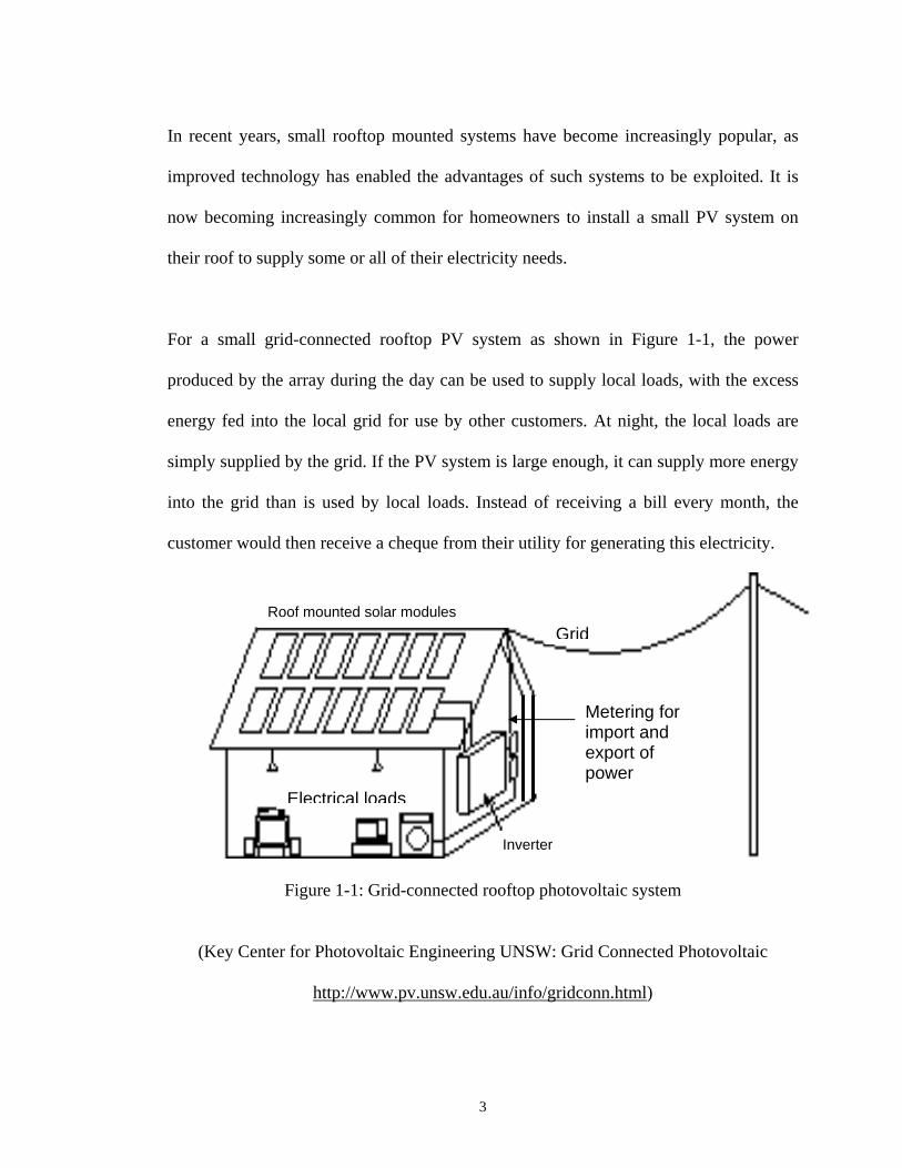
In recent years, small rooftop mounted systems have become increasingly popular, as
improved technology has enabled the advantages of such systems to be exploited. It is
now becoming increasingly common for homeowners to install a small PV system on
their roof to supply some or all of their electricity needs.
For a small grid-connected rooftop PV system as shown in Figure 1-1, the power
produced by the array during the day can be used to supply local loads, with the excess
energy fed into the local grid for use by other customers. At night, the local loads are
simply supplied by the grid. If the PV system is large enough, it can supply more energy
into the grid than is used by local loads. Instead of receiving a bill every month, the
customer would then receive a cheque from their utility for generating this electricity.
Roof mounted solar modules Grid
Metering for import and export of power
Electrical loads
Inverter
Figure 1-1: Grid-connected rooftop photovoltaic system
(Key Center for Photovoltaic Engineering UNSW: Grid Connected Photovoltaic
http://www.pv.unsw.edu.au/info/gridconn.html)
3

Distributed grid-connected PV systems offer many benefits to both the owner of the
system and the utility network. For many owners, the main attractions of such a system
are self-sufficiency and the environmental benefits of using renewable energy. The
simplicity of the system also means the owner does not need energy storage in the form
of batteries-essentially the grid is acting as a storage device. Being a modular system, it
can also expand easily as requirements or available capital grow.
The modularity of PV systems offers further benefits. The production costs for some PV
system components are related to volume of production, meaning that a large number of
small identical components can be cheaper to make than one big component. This means
that a small PV system can be as cheap or in some cases cheaper than a large system.
Furthermore, the many small systems can be distributed throughout an electricity
network rather than centralized in one location. This allows the electricity utility to take
advantage of locations where the value of electricity is greater, such as at the end of a
long and inefficient transmission line.
A grid connected PV system offers other potential cost advantages when placed at the
end of a transmission line, since it reduces transmission and distribution losses and helps
stabilize line voltage. PV systems can also be used to improve the quality of supply by
reducing 'noise' or providing reactive power conditioning on a transmission line. When
all these advantages are considered, well-positioned grid-connected PV systems are
already economically viable, even though further cost reductions are required to make
PV systems economic over the entire electricity network.
4

Many utilities are developing buy-back policies that ensure private generators are paid
fairly for the electricity they sell, with some opting for rate-based incentive schemes,
while other bodies prefer net metering or avoided cost payments. The NSW electricity
distributor Integral Energy has initiated one of the more promising energy buy-back
schemes in Australia. It uses the net metering process, but if the PV system produces
more electricity than required by the site, Integral Energy will buy back the excess at a
rate marginally lower than the standard electricity retail rate.
The main technical advance that has made grid connection of small PV systems feasible
is the availability of low-cost high-quality inverters. These inverters convert the DC
electricity generated by the PV system into AC grid electricity. Recent developments
have been towards even smaller low-cost units that can be individually incorporated into
PV modules. Built-in electronics would then allow such "AC modules" to be
interconnected and grid-connected with a minimum of costly external circuitry or
protection equipment.
A variety of grid-connected PV systems have been installed throughout the world. In
1990, Germany began its "1000 Rooftops Program" which saw 1-4 kW PV systems
installed on each of 2 250 residences. In 1997, Japan is installing 3 kW systems on 9 400
rooftops, while the USA has gone one better by announcing plans to but PV system on
1 000 000 rooftops. In these and other projects involving commercial buildings, PV cells
are being incorporated into roofing materials, cladding and windows. System cost can be
further reduced in this way by offsetting them against the cost of building materials.
5

1.1 Project Overview
In this project, a circuit diagram for grid-connected photovoltaic is design. For a house,
it is sufficient to use a 2 kW inverter. The inverter is simulated as a pulse- width
modulated voltage source operating with bipolar switching. The pulse-width-
modulation technique, which compares the fundamental frequency with the carrier
frequency is used to overcome switching losses.
In order to simulate the circuits and to validate the design process PSCAD simulation
software is used. Power System Computer Aided Design (PSCAD) is graphical based
design software that allows the design and simulation of power systems and power
electronics components. It allows the viewing of output graphs of any features in the
system including internal component parameters.
1.2 Computer Simulation
Traditionally, analogue simulators have been used in the simulation of large power
networks. Analogue simulators use passive components such as inductors, capacitors
and resistors arranged to represent the electrical characteristics of power system
components. These approximate models of power system components are then
interconnected to form a complete model of the system. This type of computer
6

simulation operates in real-time mode since the source models operate at real-time
frequency.
In this project, the computer simulation package is based on electromagnetic transient
software. The modelling capabilities of modern electromagnetic transient software such
as EMTDC are capable of representing power systems in much greater detail than
analogue simulators. EMTDC relies on mathematical models to represent power system
components.
1.3 Project Aims
The primary concern of this project is to analyse the grid-connected photovoltaic. The
aims of this project is identified as follows:
Improvements with respect to Solar Energy conversion into Electrical Energy
Computer simulation of the Photovoltaic–Grid system for performance analysis.
Study of Dynamic behavior of Photovoltaic-Grid energy systems under disturbance
Study of Grid-Connected Photovoltaic/Diesel Energy Systems.
7

CHAPTER 2
LITERATURE CRITICAL REVIEW
2.0 Introduction
The heart of the solar photovoltaic (PV) energy system is the photovoltaic device. The
photovoltaic device is a high-technology approach to converting electrical energy. The
electricity generated by a PV device is direct current (DC) and it can be used in DC form
or can be converted to alternating current (AC). PV-generated electricity can also be
stored in a storage device for later use.
Conceptually, in its simplest form a PV device is a solar-powered battery whose only
consumable is the light that fuels it. There are no moving parts; operation is
environmentally benign and if the device is correctly encapsulated against the
environment, there us nothing to wear out. Photovoltaic devices have many additional
benefits that make them useable and environmentally acceptable.
Photovoltaic systems are modular and so their electrical power output can be engineered
for virtually any application form from low-powered consumer uses to energy-
significant requirements such as generating power at electric utility central power
8

stations. Moreover, incremental power additional are easily accommodated in
photovoltaic systems unlike in more conventional approaches which use fossil or nuclear
fuel and require multi-megawatt plants to be economically feasible.
There are two types of PV technologies commercially available. These are crystalline
silicon and thin film. In crystalline-silicon technologies, individual PV cells are cut from
large single crystals. In thin-film PV technologies, the PV material is deposited on glass
or thin metal that mechanically supports the cell or module. Thin metal mechanically
supports the cell or module. Thin film-based modules are produced in sheets that are
sized for specified electrical outputs.
To understand the many facts of photovoltaic energy, we need to understand the
fundamentals of how the PV devices work. Although photovoltaic cells come in a
variety of forms, the most common structure is a semiconductor material into which a
large –area diode or p-n junction has been formed. The fabrication processes tend to be
traditional semiconductor approaches such as diffusion, ion implantation and so on.
Electrical current is taken from the device through a grid contact structure on the front of
the cell that allows the sunlight to enter the solar cell, a contact on the back that
completes the circuit and an anti-reflection coating that minimizes the amount of
sunlight reflecting from the device. The fabrication of the p-n junction is the key to the
successful operation of the photovoltaic devices.
9

2.1 Photovoltaic
Photovoltaic describes a technology, in which radiant energy from the sun is converted
to direct current (dc) electricity as shown in Figure 2-1. Although the scientific basis of
the photovoltaic effect has been known for nearly 150 years, the modern photovoltaic
cell was not developed until 1954. Only four years later the first cells were providing
power for U.S. spacecraft. Some of these early systems are still operating in space today
and attest to the reliability and durability of the technology.
Figure 2-1: Convert energy to dc electricity
Most solar cells are made of silicon semiconductor material treated with special
additives. When the sunlight strikes the cells, a flow of electrons is generated
10

proportional to the intensity of the sunlight and the area of the cell. A solar cell 10
centimeter a side will produce about 3.5 amperes in full sunlight. Each solar cell
produces approximately one-half volt. Higher voltages are obtained by connecting the
solar cells in series. The typical photovoltaic module used for terrestrial applications
contains 36 silicon solar cells, connected in series to provide enough voltage to charge a
12-volt battery. The series-connected solar cells are encapsulated and sealed, most with
a tempered glass cover and a soft plastic backing sheet. The laminated module protects
the electrical circuits from the environment and gives the long life that photovoltaic
modules are noted for. Modules may be connected in series to obtain required system
voltages or in parallel to obtain higher currents.
2.2 Cells, Modules and Panels
The photovoltaic hierarchy is shown in Figure 2-2. The Photovoltaic electricity is
produced by an array of individual PV modules electrically connected in series and
parallel to deliver the desired voltage and current. Each PV module, in turn, is
constructed of individual solar cells also connected in series and parallel. A typical
crystalline silicon solar cell is 100 cm2 and produces about 1.75 peak watts (Wp) at 0.5
volt and 3.5 amps under full sun at standard test conditions (STC: 1,000 W/m2 and 25ºC
cell temperature).
11

Dozens of solar cells are connected together to produce a PV module. The number of
cells determines a module's size and power. Cells and modules connected electrically in
series build voltage while cells and modules wired in parallel build current.
Figure 2-2: Photovoltaic hierarchy
(Tomas Markvart and Klaus Bogus: Solar electricity: 2nd Edition)
There are two basic types of PV modules commercially available today: those made
from crystalline silicon and those made from amorphous silicon. Crystalline silicon
modules are presently the dominant commercial product and deliver approximately 100-
120 W / m2 at STC. Amorphous silicon (a-Si) thin-film modules, which are beginning to
enter the market, require less material to produce than the thick crystalline products and
so can be made less expensively. Today's commercial a-Si modules deliver 40-50 W /
m2 under full sun at STC. Other thin-film PV materials such as copper- indium-
diselinide (CIS) and cadmium telluride (CdTe) are currently under development and
hold the promise of lower costs in the future.
12

When designing a PV system, one or more of the following parameters determines the
array size: available aperture area, available resources (both solar and financial), and the
load requirements. The array's operating voltage will determine, or be determined by the
dc input voltage requirement of the inverter. Figure 2-3 illustrates the grid-connected
photovoltaic array.
RETE
CARICO
Figure 2-3: Grid-connected photovoltaic array
2.3 Technical Explanation Of Photovoltaic Cells
13

A single PV cell is a thin semiconductor wafer, generally made of highly purified
silicon. The wafer has been doped on one side with atoms that produce a surplus of
electrons and the other side with atoms producing a deficit of electrons. This establishes
a voltage difference between the two sides of the wafer. In silicon this is just under half
a volt. Metallic contacts are made to both sides of the wafer. When the wafer is
bombarded by the photons in sunlight, electrons are knocked off the silicon atoms and
are drawn to one side of the wafer by the voltage difference. If an external circuit is
attached to the contacts, the electrons have a way to get back to where they came from
and a current flows through the circuit. The PV cell acts like an electron pump. The
amount of current is determined by the number of electrons that the solar photons knock
off the silicon atoms, so by the size of the cell, the amount of light on the cell and the
efficiency of the cell.
A PV module consists of many cells wired in parallel to increase current and in series to
produce a higher voltage. Modules consisting of 36 cells in series have become the
industry standard for large power production. The module is encapsulated with tempered
glass (or some other transparent material) on the front surface, and with a protective and
waterproof material on the back surface. The edges are sealed for weatherproofing, and
there is often an aluminum frame holding everything together in a mountable unit. A
junction box, or wire leads, providing electrical connections is usually found on the
module's back. Although truly weatherproof encapsulation was a problem with the early
modules assembled 15 years ago, we have not seen any encapsulation problems with
glass-faced modules in many years.
14

PV costs are now down to a level that makes them the clear choice for most remote, and
many not so remote, power applications. They are routinely used for roadside
emergency phones and many temporary construction signs, where the cost and trouble of
bringing in utility power outweighs the higher initial expense of PV, and where mobile
generator sets present more fueling and maintenance trouble. More than 100,000 homes
in the United States, largely in rural sites, now depend on PVs as a primary power
source, and this figure is growing rapidly as people begin to understand how clean and
reliable this power source is, and how deeply our current energy practices are borrowing
from our children. Because they don't rely on miles of exposed wires, residential PV
systems are more reliable than utilities, particularly when the weather gets nasty. PV
modules have no moving parts, degrade very, very slowly, and boast a lifespan that isn't
fully known yet, but will be measured in decades. Standard factory warranties are
usually 10 years, with some manufacturers offering up to 25-year warranties. Compare
this to any other consumer goods, or power generation technology.
2.4 How Does Solar Cell Works?
15

Figure 2-4, illustrate the overview of how solar cell works. The photovoltaic effect is the
release of electron from semi-conductors when falls on their surface. A typical solar cell
consists of two layers of treated silicon; P-type and N-type silicon. P-type silicon has
unbound positive charges. N-type silicon has free negative charges. When the sunlight
hits the solar cell, they P-type and N-type silicon move apart. This movement creates a
direct current and generates voltage
Figure 2-4: How solar cell works
(U.S. Department of Energy Photovoltaic Program: Turning Sunlight Into Electricity
http://www.eren.doe.gov/pv/conveff.html (1st December 2001))
16

2.5 DESCRIPTION OF PHOTOVOLTAIC ARRAY MODEL
The model of the photovoltaic array is based on the well-known single-diode
representation of a silicon photovoltaic cell as shown in Figure 2-5.
Figure 2-5: Equivalent circuit of a photovoltaic cell
(Renewable Energy 304: Lecture Notes)
Component-specific parameters:
(Note: Model parameters for the BP 280 PV module are shown in brackets)
Ior Inverse diode saturation current at reference temperature
[ Ior = 3.047e-7 A ]
ISCR Short-circuit current under STC [ ISCR = 4.92 A]
It Short-circuit current temperature coefficient [ It = 1.7 e-7 A/°K ]
A Diode ideality factor [ A = 1.403 ]
Tr Cell reference temperature [ Tr = 300 °K ]
17

NOCT Normal operation cell temperature [ NOCT = 43 °C ]
EG Bandgap for semiconductor material [EG (Si) = 1.11 eV ]
RSH Cell shunt resistance [ RSH = 50 Ω ]
RS Cell series resistance [RS=50 mΩ]
NS Number of cells in series [NS = 36]
NP Number of cells in parallel [NP = 1]
The governing equations, describing the I-V characteristics of a crystalline silicon
photovoltaic cell are represented in the following. The light-generated current is given
as:
ILG = ISR x GN +It (Tc –Tr) (1)
where the normalized irradiance GN is calculated from
The diode current of the photovoltaic cell is calculated as:
where the inverse saturation current of the pn junction is expressed as:
2/1000 mWGGN = (2)
( )
⎥⎤
⎢⎡
−=+
1PVCSPVC
c
IRV
AkTq
eII (3) ⎥⎦
⎢⎣
oD
⎟⎠
⎜⎝
⎟⎟⎠
⎜⎜⎝
= cr TTAk
r
coro e
TII (4)
⎟⎞
⎜⎛
−⎞⎛ GqET
113
18

The current due to the shunt resistance of the photovoltaic cell can be expressed as:
SH
SPVCPVCRSH R
RIVI
+= (5)
Therefore, the photovoltaic cell current is given as:
IPVC = ISRGN +It (Tc –Tr) - ID –IRSH (6)
(7) ( )
SH
SPVCPVCDrctNPVC R
RIVITTIGII
SCR
+−−−+=
Inspection of equation (7) shows that the photovoltaic cell current is a function of itself,
forming an algebraic loop, which can be solved conveniently using SIMULINK.
Alternatively, it is possible to neglect the influence of the series resistance (RS=0Ω) to
derive a simplified equation for the photovoltaic cell current. The cell temperature is
calculated as :
( )CNOCTGTT oac 20
800−+= (8)
A photovoltaic module can be modeled as a series/parallel connection of cells as
expressed by the following equations for the photovoltaic module voltage and current,
respectively
19

PVCSPVM xVNV = (9)
PVCPPVM xINI = (10)
Similarly, a photovoltaic array is represented by the number of modules connected in
series Ms and the number of modules in parallel MP, where the photovoltaic array
voltage and current are given as:
PVCSSPVMSPVA xVxNMxVMV == (11)
(12) PVCPPPVMPPVA xIxNMxIMI ==
Therefore, the photovoltaic cell voltage is calculated from the photovoltaic array
voltage, which is an input to the photovoltaic array model:
SS
PVAPVC NM
VV = (13)
When calculating the photovoltaic array current, the cell current is multiplied by the
number of strings of cells in parallel for each module as well as the number of module
strings in parallel, as expressed by equation (12).
This model of the photovoltaic array does not account for variations of the performance
of individual cells, shading effects or wiring losses.
20

2.6 What Is Power Point Tracking and Is It Worth the Expense?
The output of a PV module is characterized by a performance curve of voltage versus
current, (I-V curve) as shown in Figure 7. The maximum power point of a PV module is
the point along the I-V curve that corresponds to the maximum output power possible
for the module. This value can be determined by finding the maximum area under the
current versus voltage curve. The maximum power point for standard test conditions of
1000W/m2 and 25C with air mass of 1.5 is shown in Figure 2-6 to have about 17.4 volts
and 2.5Amps.
Typical I-V Curve @ 25°C for Silicon Module
Maximum Power Point, Vmp & Imp
Isc, Short circuit current
Imp
Vdischarge
Volts
Open circuit voltage,VocVmp
Figure 2-6: Typical I-V Curve
21

For crystalline modules, the current remains fairly constant as the voltage moves up and
down throughout the typical battery voltage ranges. In PV systems that charge a battery,
the battery to which it is connected determines the module output voltage. Should the
battery be at a low state-of-charge, the output voltage of the PV module will be reduced
in voltage, and hence the module output wattage is reduced. (See V discharge on Figure
2-6) With a battery discharged to 11.0V, a corresponding module current of 2.6A can be
realized, which is only 66% of the available module power.
Maximum power point tracking enables a PV module, or array, to operate at its
maximum power point while charging a battery at a lower voltage, in this instance the
module can produce 43.5W instead of 28.6W. There are several factors that will
influence the amount of power gain one can expect; these factors are cell temperature,
conversion losses, amount of available sunlight, cell structure, battery voltage, and
blocking diodes. Some power is lost in the conversion from the voltage at the maximum
power point to battery voltage. The efficiency of most maximum power point tracking
units is usually around 93%.
Some maximum power point trackers, like the Fire Wind and Rain unit, will have an
automatic bypass that will allow the charge controller to use the battery voltage as the
module output voltage if the conversion takes more power than is being gained by using
maximum power point tracking.
22

For crystalline modules, voltage will drop about 2.4mV per degree C per cell. A 36-cell
module on a typical summer day in Kingston, NY will have a cell temperature of 45C
during peak sun hours. This yields a voltage drop of 1.73V, and shifts the I-V shown in
Figure 7 thus lowering the maximum power point closer to the battery voltage. As
sunlight diminishes from the standard test condition of 1000W/m2, the voltage
corresponding to the maximum power point drops slightly, but the main component in
the decrease of available power is the decrease in available current.
In the case of amorphous silicon modules, the I-V curve will change current more
dramatically as the voltage changes throughout the battery voltage and maximum power
point ranges. This will translate into less gain seen by using the maximum power point
tracker.
Battery voltage will also play a major role in the amount of increased watt-hours one can
expect from a module or array using a maximum power point tracker. If the battery bank
is mostly near a full state-of-charge, then the voltage of the battery bank will be closer to
the maximum power point voltage and very little gain will be seen using the maximum
power point tracker. The use of blocking diodes will also mandate that the module be 0.3
to 0.7 volts higher than the battery voltage, thus lessening the difference between battery
voltage and voltage at the maximum power point.
When does using a maximum power point tracker make sense? The typical wattage gain
using a maximum power point tracker is 10 to 13%. Therefore, for systems under 300W,
23

it is usually more cost effective to buy another module than to buy a maximum power
point tracker. However, for systems above 300W the additional cost of the maximum
power point tracker can more than pay for itself with increased watt-hour output from
the array. Also, the percentage gain is greater in the winter, when the air temperature is
colder (thus colder cell temperature and higher max power point voltage), and this is
when the added array output is most needed. Recently there have been several
manufacturers that are marketing several relatively inexpensive units that will find a
home in many PV designs to come.
2.7 Photovoltaic (PV) System
Solar cells are made of certain semiconductor materials, which produce a voltage when
exposed to light. Small wires are placed on the semiconductor to provide a path for the
flow of direct current (DC) electricity. As more light falls on a cell, more electricity is
generated; therefore, a PV system must not be shaded (i.e. by shadows, snow, or wet
leaves) because such shading can substantially reduce performance.
A typical solar cell made of crystalline silicon is 4 inches in diameter and 0.010 of an
inch thick. In direct sunlight, it generates 2 amperes of direct current at 0.5 volts. By
connecting solar cells in series (to increase the voltage), and in parallel (to increase the
24

current), the output of a PV system can match the requirements of the load to be
powered. If more power is required, modules can be appropriately connected in series or
parallel to form what is called a PV array (see Figure 2-7).
Figure 2-7: Residential photovoltaic system
Having the solar cells track the sun as it moves across the sky can increase the total
energy output of a PV system. Concentrating mirrors and lenses can also be used to
increase output. These more complex systems are promising, but the additional cost
must be evaluated on a case-by-case basis.
Most current PV installations are for power requirements in locations remote to existing
power lines. In some instances, such as radio communications equipment on top of
mountains, photovoltaics may be the only reasonable means of supplying power.
25

However, distance from a power line is not always the controlling factor. For example,
even if a power line is located in close proximity to a small load (such as an emergency
call box), it is often more economical to use PV power instead of running a special line
to the box.
2.8 Use of Photovoltaic (PV)
Electric power generation options are now starting to be compared on a basis that
includes "externalities." Externalities are the "hidden" costs associated with a power
source that are not accounted for in the price of the power produced. These hidden costs
include damage to the environment caused by the sourcing, processing, transporting,
using, and disposal aspects of a power source. The operational costs and externalities
associated with the conventional fuel mix (coal, oil, nuclear, natural gas) used for
generating electricity are not substantially less than the "full" costs associated with
photovoltaic systems and, in many cases, exceed the costs of PV's. The use of PV's is
much less polluting than other fuel choices. Refer to Figure 2-8 for the comparison of
Commercial Status and Implementation Status.
The primary strategy for use of PV's as the electrical power source for a residence is
reducing the need for electricity. Refrigerators, air conditioners, electric water heaters,
electric ranges, electric dryers, and clothes washers are all large users of electricity.
26

Highly energy conserving alternatives and gas appliances are available to greatly reduce
electrical loads.
Figure 2-8: Comparison of Commercial Status and Implementation Status
27

2.9 Advantages Of Photovoltaic (PV) System
Photovoltaic offers advantages over diesel generators, batteries and conventional utility
power.
High reliability:
Photovoltaic cells were originally developed for use in space where repair is
extremely expensive and difficult if not impossible. Photovoltaic systems still
power nearly every satellite circling the earth because they operate reliably for long
periods of time with virtually no maintenance.
Low operating costs:
Photovoltaic cells use the energy from the sunlight to produce electricity-the fuel is
free. With no moving parts, the cells require little maintenance. These low
maintenance, cost effective photovoltaic systems are ideal for supplying power to
communication stations on mountain tops, navigational buoys at sea or homes far
from utility power lines.
No pollution:
Because they burn no fuel and have no moving parts, photovoltaic systems are clean
and silent. This is especially important where the main alternatives for obtaining
power and light are from diesel generators.
28

Modular:
A photovoltaic system can be constructed to any size. Furthermore, the owner of a
photovoltaic system can enlarge it if his or her energy needs increase. For instance,
homeowners can add modules every few years as their energy needs and financial
resources grow.
Low construction costs:
Photovoltaic systems are usually placed close to where the electricity is used. This
means that a much shorter wire is required than if power is brought in from a utility
grid. Fewer wires mean lower costs, shorter construction time and a reduction in
paperwork as permits do not need to be applied for, particularly in urban areas. In
addition, using photovoltaic eliminates the need for a step-down transformer from
the utility line. The photovoltaic system makes the traditional requirements of
building large, expensive power plants and distribution systems unnecessary.
29

CHAPTER 3
GRID-CONNECTED PHOTOVOLTAIC (PV) SYSTEMS
3.0 Introduction
Grid-connected systems are sometimes referred to as cogeneration systems. They
normally do not include batteries. Here, the inverter must be capable of accepting the
full range of solar array voltage and power excursions, and must be capable of operating
at the array peak-power point instantaneously. In this case, the utility network acts as an
infinite energy sink and accepts all available power from the PV system. The simplest
grid-connected system has a PV array and an inverter as in the case of low-voltage
residential grid connection as shown in Figure 3-1. For high-voltage grid-connected
systems (greater than 220 or 380 Vac), transformers and appropriate power switching and
protection devices are included.
Figure 3-1: Grid-Connected PV Configuration, without battery
(Ahmed Zahedi: Solar Photovoltaic Energy Systems: Design and Use)
30

Grid-connected systems, power factor correction and harmonic filtering devices are
essential. However, the grid-interface criteria vary with the utility companies and have
yet to be standardized internationally. Most of the inverters now being used for grid-
connected applications incorporate peak-power tracking capability. Those inverter
controls the PV array output to maintain operation at its maximum power point, which
changes rapidly with variations in solar intensity and module temperature.
3.1 Grid-Connected Photovoltaic (PV) Systems
The load in such plants is the utility network, and the usual assumption here is that the
grid is capable of accepting any amount of power from the PV plant. In other words, the
utility grid serves as an infinite energy sink. The utility company dictates the
requirements for the grid-connected system, and each utility may impose a unique set of
requirements. The main grid interface criteria, which should be checked with the utility,
are the following:
Voltage regulation
Frequency regulation (usually 2% of nominal)
Harmonic distortion in the operating load range:
31

⇒ Total of all current harmonics (usually 5% maximum)
⇒ Any single current harmonic (usually 3% maximum)
⇒ Total of all voltage harmonics (usually 5% maximum)
Power factor and reactive power consumption:
⇒ Utilities often stipulate a power factor requirement for co generators, from
0.9 lagging to 0.9 leading at full load.
⇒ Reactive power consumption is closely related to the power factor (PP).
Typical residential and industrial loads operate with a lagging PF as low as
0.85. Because of this, the utility requires some power factor correction by
co-generating sources to minimize reactive power being supplied by the
grid. The inverters used in the PV system consume reactive power and thus,
the utility could lose revenue due to real-power line losses.
Protection and operation criteria such as:
⇒ Inverter disconnect criteria in the event of a grid failure (loss of voltage),
inverter failure, or a ground fault on the dc side
⇒ Inverter reconnects criteria
⇒ Adequate safeguard against "islanding" (inability of self-commutated
inverters to detect grid shut-down so that they continue to operate and feed
power into the grid)
32

3.2 Performance Calculator For Grid-Connected PV Systems
Fixed or tracking array
The PV array may either be fixed, sun-tracking with one axis of rotation, or sun-
tracking with two axes of rotation. The default value is a fixed PV array.
Figure 3-2: PV Array Orientation
(Stuart R. Wenham, Martin A. Green and Muriel E. Watt: Applied Photovoltaic)
PV array tilt angle (0° to 90°)
For a fixed PV array, the tilt angle is the angle from horizontal of the inclination of
the PV array (0° = horizontal, 90° = vertical). For a sun-tracking PV array with one
axis of rotation, the tilt angle is the angle from horizontal of the inclination of the
tracker axis. The tilt angle is not applicable for sun-tracking PV arrays with two
axes of rotation. The default value is a tilt angle equal to the station's latitude. This
33

normally maximizes annual energy production. Increasing the tilt angle favors
energy production in the winter, while decreasing the tilt angle favors energy
production in the summer. For roof-mounted PV arrays, Table 3-1 below gives tilt
angles for various roof pitches (ratio of vertical rise to horizontal run).
Roof Pitch Tilt Angle (°)
4/12 18.4
5/12 22.6
6/12 26.6
7/12 30.3
8/12 33.7
9/12 36.9
10/12 39.8
11/12 42.5
12/12 45.0
Table 3-1: Tilt angles for various roof pitches
34

PV array azimuth angle (0° to 360°)
For a fixed PV array, the azimuth angle is the angle clockwise from north of the
direction that the PV array faces. For a sun-tracking PV array with one axis of
rotation, the azimuth angle is the angle clockwise from north of the direction of the
axis of rotation. The azimuth angle is not applicable for sun-tracking PV arrays with
two axes of rotation. The default value is an azimuth angle of 180° (south-facing).
This normally maximizes energy production. Increasing the azimuth angle favors
afternoon energy production, while decreasing the azimuth angle favors morning
energy production. Table 3-2 below provides azimuth angles for various compass
headings.
Compass Heading Azimuth Angle (°)
N 0 or 360
NE 45
E 90
SE 135
S 180
SW 225
W 270
NW 315
Table 3-2: Azimuth angles for various compass headings
35

3.3 Grid-Connected Inverter Photovoltaics
Various inverter topologies used Conditioners may produce different degree of quality
of AC power output. While PV/Diesel system can operate in stand-alone mode, it can
also be connected through a line inductor to the Grid as an UPS system. Integrated
Solar/Mains/Diesel system has several desired features such as UPS function, peak
shaving function, Power Conditioning of weak grid supply, Active filtering, Voltage
regulation at critical loads etc.
Figure 3-3: Grid-connected inverter photovoltaic
(Western Power 2000)
36

3.4 Grid-Connected Inverter Photovoltaics (Characteristics)
Figure 3-4: Grid-connected inverter (Characteristics)
(Western Power Specification)
Table 3-3 below summaries the grid-connected inverter characteristics, which explain
Figure 3-4. These characteristics are essential in designing inverters under Western
Power Specifications.
Response Times Very fast-milliseconds
Harmonic Output Very low, computer more noisy
Synchronisation Automatic-Within couple of cycles
Frequency Control Locked to grid
Power Factor Close to unity, can help regulate mains
Fault Currents Low-PV, similar to normal appliances
DC Injection Avoid-Transformer and detection
Islanding Use passive and active protection methods
Table 3-3: Grid-connected inverter characteristics
37

3.5 Grid-Connected Inverter (Standard and Regulation)
ESAA (Draft) Western Power (Draft)
Evolving
Standard Contents: Operating Limits-Voltage 200-270V Quality- Harmonics-Aust Standards
Power Factor-Close to Utility Voltage Flicker-WP Quality req
Protection-Passive-Under/Over Voltage Under/Over Frequency
Other
Active- Frequency Bias Impedance Measurement Reactive Power Modulation Load Switching Safety- Type Tested Approved Inverters Installed Requirements Testing Labeling Office of Energy-Reporting
Grid Connected Standard
Figure 3-5: Grid-connected inverter (Standards and regulations)
(Western Power)
38

CHAPTER 4
SOFTWARE ANALYSIS
4.0 PSCAD/EMTDC The EMTDC program is developed to evaluate concepts, ideas and models portions of
planned or existing power systems. The tasks required to set-up, run, and analyse the
results of a simulation is further simplified with the development of PSCAD, a graphical
user interface for EMTDC furthermore EMTDC does all the calculations required. The
interface between PSCAD and EMTDC is shown in Figure 4-1.
File Manager
Draft TX Line/Cable Run Time Multi-Plot
Information
EMTDCProgram
OutputFiles
Data
Figure 4-1: Interface of PSCAD and EMTDC
39

Multiple simulator architectures such as EMTDC can be supported by PSCAD. The
"Draft" and "RunTime " modules are quite similar, diversity between these two modules
depends solely on the simulator architecture. The two modules are capable of switching
between these architectures after start-up and by specifying default simulator
architecture in the "File Manager", adds convenience to this software. This value will be
passed to the "Draft" and "Runtime" modules on program startup. The "Draft",
"RunTime" and "MultiPlot" functions are discussed in more detail following section.
4.1 Draft
A power system circuit layout module called “Draft” in PCSAD enables the user to draw
graphical representations of power systems. These graphical representations are
analysed which results in the creation of simulation data files for PSCAD's "Runtime"
executive modules.
Procedure of opening the "Draft" from "File Manager" module are firstly, open the
desired project/case directory then select the "Draft" button from the File Manager's
Process Area. The "Draft" module contains several different areas in which the three
most important areas are:
40

Top Menu Area - contains controls for the global functions of the module
Drawing Canvas - the power system to be simulated is drawn in this region
Component Palette - contains components used to draw the power system
"Help" button found on the top menu enable the user to learnt more about the “DRAFT"
module.
A "Draft" circuit drawing or system can have many pages known as " subsystems ". The
name and comment of each individual subsystem can be entered on the "subsystem
properties form", which is accessible using the "PROERPTIES" item on the
"SUBSYSTEM" menu.
Printing of the circuit that has been drawn can be done easily, simply select the
"POSTSCRIPT" option of the "PRINT" menu. The same procedure applies if the user
choses to save the circuit drawn simply select the “File” menu and then save.
To compile the circuit, select the "COMPILE" option, which will produce all files
necessary to run the simulation. An error free system will produce a text saying that
"Compile complete, with 0 error(s) 0 warning(s)" which will appear in the message box
along the bottom edge of the "Draft" window. Nevertheless, if there are errors, error
warnings explaining the source of the errors will appear. Check through the errors and
rectify them before compiling it again. Once its all clear, the next step would be to
"Run" them, which bring us to the "Runtime" simulations.
41

4.2 Runtime
A module for managing, controlling and interfacing with multiple power system
simulations cases, each of which may be running on any of the computer system's
support architectures in the EMTDC system is called “RUNTIME”.
Starting the "Runtime" from the "File Manager" module, consist of the same procedure
when the user wants to start the “DRAFT” module. Open the desired project/case
directory, and select the "Runtime" button from the File Manager's Process Area. When
"Runtime" is selected, a single EMTDC Operator's Console window is automatically
created and displayed. Listed below is the information required in order to simulate a
power system circuit from the EMTDC Operator's Console.
The EMTDC library dimension version to use
The Fortran dynamics and output subroutine filenames, as well as any other
subroutine files to be included.
The information file and the starting data or snapshot file.
As these items are a requirement, the "Draft" module will creates a "Runtime" batch file
with default information when a system is recompiled
To load the "Batch" file, just select "Load" option from "Batch" menu. Then select the
file that is meant for loading and then click "Proceed".
42

To simulate the system, select "Plot" option in the "Create" menu. This will open the
plot component's "Properties Form", where the required data to be simulated is selected
and the appearance of the plot may be controlled. Click " Proceed" after everything is
done. To run the simulation clicks the play button. Along side the play button, there are
other control buttons that controls the status of the simulation like the start, pause, single
step and stop. To print out the graphs simulated, just go to "MultiPlot".
4.3 MultiPlot
“MULTIPLOT” is available in the system for printing the required waveforms. It has a
flexible interface, which enables the user to create multi page arrangements, each page
containing any number of graphs and text labels, and each graph containing any number
of data channels.
To start "MulitPlot" from the "File Manager" module, the desired project/case directory
is opened and "MultiPlot" is selected form the File Manager's Process Area. The are two
main screens subdivision in "MultiPlot" are:
Top menu area of the "Multiplot" window contains menus and buttons which
provides access to various operations
Work area where the graphs are to be displayed and manipulated.
43

CHAPTER 5
MODELLING OF GRID-CONNECTED PHOTOVOLTAIC
5.0 Introduction
A true inverter takes power from a fixed dc source and applies it to an ac load such as a
utility grid, an ac motor, a loudspeaker or a conventional product normally powered
from an ac line. It is useful to distinguish two types of ac loads, active and passive.
The utility grid is the most familiar active ac load. The utility waveform is controlled
very precisely at a central location. A converter connected to the grid cannot alter the
timing of the sinusoid. Hence, phase delay control is used as the adjustment tool.
Real ac loads often include magnetic transformers, which only function with ac signals.
If dc voltage is imposed on a transformer, it can cause the flux to increase until the
device no longer functions. This is the key consideration in inverters: Any dc component
is unwanted and in fact can cause considerable trouble. A practical inverter circuits
should not produce any dc output component.
44

Figure 5-1 shows a 2 x 2 switch matrix to transfer energy from the dc voltage
source into an ac current source. This circuit is referred to as a full-bridge
inverter. The switches must carry bi-directional current. The voltage source is
unidirectional so only one blocking direction is required. Inverter applications
usually use some type of transistor with reverse-parallel diode to give it bi-
directional current capability. Today, the power MOSFET is used up to 1-10kW,
while IGBTs are used at power levels up to 100kW. For even higher levels,
GTOs with reverse-parallel diodes can be substituted. Therefore, MOSFET is
used to design 2kW DC to AC inverter.
Vin
iac(t)
Figure 5-1: Switch matrix for dc voltage to ac current conversion
The inverter is simulated as a pulse-width modulation (PWM) modulated inverter with
bipolar voltage switching and is voltage sourced. For this inverter type a modulating
sinewave control signal at the desired output frequency is compared to a triangular
waveform, the frequency of which established the inverter switching frequency. This
carrier frequency is generally kept constant.
45

5.1 Schematic of PV System for household electrification
The schematic of PV-system for household electrification is illustrated in 5-2. The solar-
cell modules rest on an array support structure. The array support structure is generally
made out of aluminium or steel struts, resting on a concrete foundation. At the present
most systems have fixed arrays. In case of a tracking system it must keep the modules in
an optimal orientation towards the sun. There are several options.
Seasonally-adjusted tilt. A few times a year the arrays can be adjusted to the
elevation of the sun.
Single-axis or two-axis tracking. A drive mechanism keeps the modules in the
direction of the sun during the whole day. The array structure can rotate in one or
two directions.
The power conditioning can be composed of the following elements:
Controllers
Maximum power point tracking
DC-AC converters
Interface between the PV-system and the grid
Electronic protection of the system.
46

Sun Photovoltaic Array
Controller/Regulator
Lighting
Battery
Refrigerator Radio Fan
Figure 5-2: Schematic of PV-System for household electrification
(Solar Energie Technik:
http://www.wot.utwente.nl/ssadc/chapter5.htm)
47

5.2 Grid-Connected Photovoltaic Circuit Diagram
The grid-connected photovoltaic circuit was designed as shown in Figure 5-3. The
circuit was complied using PSCAD software. The simulated system consists of
photovoltaic modules, charge controller, MPPT, battery, inverter, grid and load.
Figure 5-3: Grid-connected photovoltaic circuit diagram
5.2.1 Photovoltaic Generations
In my design, BP 2150S PV module is chosen. The BP 2150S PV module is part of BP
Solar’s new series of 72-cell modules designed specifically for large PV systems. Its 72-
cell series string charges 24V batteries (or multiples of 24V) efficiently in virtually any
48
climate. With 150 W of nominal maximum power, it is primarily used in utility grid-
supplemental systems, telecommunication systems, pumping and irrigation, cathodic
protection, remote villages and homes and land-based navigation aids. Refer to
Appendix A for the module specifications.
5.2.2 Maximum Power Point Tracking (MPPT)
The maximum power point tracking ensures that at any given moment, with any given
amount of sunlight and any given cell temperature the maximum power is extracted
from the modules.
In general electricity is supplied as AC (alternating current). Therefore a lot of
equipment has been developed for AC-application. The PV modules, however, supply
DC (direct current)-power. The consequence is that a choice has to be made between the
use of DC-apparatus, not available for all appliances, and the installation of an inverter
to convert DC into AC. To connect a PV-system with the grid, a special interface is
needed including a DC-AC inverter. To obtain the highest possible system efficiency it
is important to lose only small amounts of energy in the power conditioning. When the
system is not working on full power the efficiency of the power conditioning does fall;
49

sometimes only about 70% efficiency is left. The cost of the power conditioning
depends on the need for AC or DC-voltages.
MPPT can be design as a step-down (buck converter), step-up (boost converter) and
buck-boost converter. However in this design, a step-down MPPT is needed to charge
the batteries. The MPPT is connected directly between the PV and battery to convert
42.8V to 24V as shown in Figure 5-4.
Figure 5-4: Step-down MPPT
where, Tt
ttt
II
VV on
offon
on
R
PV
PV
R =+
==
50

The simplified block model of a MPPT supplying a resistive load is shown in Figure 5-5
with the following parameters.
Figure 5-5: Simplified block model
RPVR
PI
RIPRIV
IVPP
mpptmppout
mpptmppout
outmpptmppoutout
outoutmpptmppout
××=
×=
×=×⇒×=
×=×=
µ
µ
µ
µ2
The typical conversion efficiency of MPPTs;
97.092.0 << mpptµ
51

5.2.3 Battery Storage
The most widely used battery in Renewable Energy System is the gel type, maintenance
free, lead acid battery. The MASTERVOLT battery is chosen in this design. The battery
bank is connected directly to the PV. The PV power output will supply power to the
loads and at the same time charging the battery. When the PV modules do not produce
enough power to the load, power will be imported from the grid. However at times of
grid failure, the battery will supply power to the load.
The initial source voltage at 24Vdc represents a series connected bank of 2, 12V units.
The battery bank incorporates a series resistance of 0.001Ω. The battery bank ensures
that a fully regulated input is available to the inverter and can provide energy storage
and power conditioning. The battery equivalent circuit is shown in Figure 5-5 with the
following parameters.
Figure 5-5: Battery equivalent circuit
(Adisa A. Jimoh and Olorunfemi Ojo, Obasohan Omozusi, “A Battery-PWM Inverter Single-Phase Induction Generator for Regulated Load Voltage and
Frequency Operation”, Vol 1, No. 2, August 1999)
52
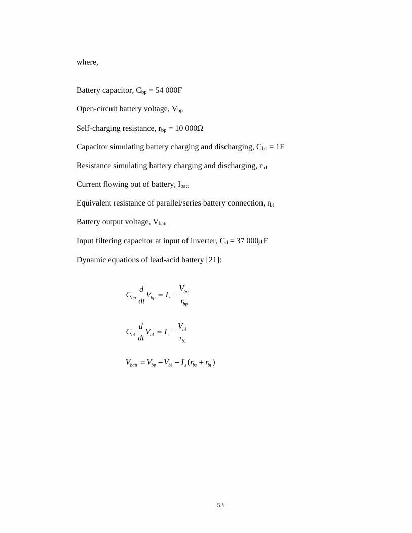
where,
Battery capacitor, Cbp = 54 000F
Open-circuit battery voltage, Vbp
Self-charging resistance, rbp = 10 000Ω
Capacitor simulating battery charging and discharging, Cb1 = 1F
Resistance simulating battery charging and discharging, rb1
Current flowing out of battery, Ibatt
Equivalent resistance of parallel/series battery connection, rbt
Battery output voltage, Vbatt
Input filtering capacitor at input of inverter, Cd = 37 000µF
Dynamic equations of lead-acid battery [21]:
)(1
1
111
btbssbbpbatt
b
bsbb
bp
bpsbpbp
rrIVVV
rVIV
dtdC
rV
IVdtdC
+−−=
−=
−=
53

5.2.4 INVERTER
There are three basic schemes of inverter, which can convert the solar module’s DC
energy into AC. The first type is step-up and chop inverter, second type is high voltage
in, only chop inverter and lastly is chop and transfer inverter. This AC may then be fed
into the grid of 240V. However, the third inverter type is chosen, as the waveform
delivered by this inverter is the only waveform allowed to be grid-connected, when the
inverter is capable of synchronization to the grid. This inverter will convert the low
voltage DC into a low voltage AC first and then converts the low-voltage AC into the
wanted AC voltage.
The advantages to this inverter are the low-voltage which is a safe operation, the
insulation from the grid after the inverter, the ease with which it makes sinewave, which
feeds into the transformer, and the most important aspect is its reliability due to the low
number of semiconductors in the power path. The inverter in my design has an
efficiency of 95%.
54

5.3 Circuit Descriptions and Specifications
The modeled grid-connected photovoltaic circuit diagram is illustrated in Figure 5-6.
The components are described and the values are specified in detailed.
Figure 5-6: Grid-connected photovoltaic circuit diagram
Components:
Resistors:
R1
Resistor R1 is required for the simulation package to obtain the PV current. The
resistance value is selected at an arbitrarily low value (R1 = 0.001Ω)
55

R2
Resistor R2 is required for the simulation package to obtain the MPPT current. The
resistance value is selected at an arbitrarily low value (R1 = 0.001Ω)
R3
Resistor R3 is required for the simulation package to obtain the battery current. The
resistance value is selected at an arbitrarily low value (R1 = 0.001Ω)
R4
Resistor R4 is required for the simulation package to obtain the secondary current. The
resistance value is selected at an arbitrarily low value (R1 = 0.001Ω)
R5
Resistor R5 represents the lighting load (R5 = 115.2 Ω)
R6
Resistor R6 is connected in series with a diode D1, which represent the computer load
(R7 = 230.4 Ω).
R7
Resistor R7 represents the motor load (R9 = 40 Ω)
R8
Resistor R8 is required for the simulation package to obtain the grid current.
The resistance value is selected at an arbitrarily low value (R8 = 0.000001 Ω)
56

Capacitors:
C1
Capacitor C1 is connected across the photovoltaic (PV) to filter off the ripple at the
output voltage. The capacitance value is selected at an arbitrarily low value (C1 =
1000µF).
C2
Capacitor C2 is connected across the battery to filter off the ripple voltage at the inverter
input. The capacitance value is selected at an arbitrarily low value (C2 = 1000µF).
C3
Capacitor C2 is connected across the secondary coil of the transformer and in addition to
inductor L1 assists in filtering high frequency components of the AC voltage waveform.
The capacitance value is selected at an arbitrarily value (C3= 100µF).
Inductors:
L1
Inductor L1 is connected in series with the primary coil of the transformer and in
addition to capacitor C2 assists in filtering high frequency components of the AC
voltage waveform. The inductance value is selected to be 542.58µH.
57

L2
Inductor L2 is connected in series with a resistor R9, which represent the motor load.
The inductance value is selected to be 0.248H
Diode:
Diode D1 is connected in series with resistor R7 represents the computer load.
Transformers:
For high-voltage grid-connected systems (i.e. greater than 220 or 380 Vac), transformer
is needed. In this circuit diagram a step-up transformer is used.
Maximum Power Point Tracking (MPPT):
A buck-converter is used to step-down the PV output voltage to the 24V nominal for
charging the battery.
Battery
Gel-type, MASTERVOLT battery is chosen. 10 of those 200Ah, 12V batteries will be
needed to provide 5 days of battery back-up at the discharge rate of 2000W per day in a
24V system.
58

Switching Transistors:
The switches are arranged to form a standard full-wave rectifier bridge. They consist of
bipolar transistors with freewheeling diodes. Switches D1 and D2 are turned on
simultaneously, whilst switches D3 and D4 are turned off simultaneously, generating the
positive half-cycle of the AC output voltage. The timing of the conduction is controlled
proportionally to the magnitude of the sinewave. Subsequently, switches D1 and D2 are
turned off simultaneously, whilst switches D3 and D4 are turned on simultaneously,
generating the negative half-cycle of the AC output voltage. The timing of the
conduction is again controlled proportionally to the magnitude of the sinewave.
Load:
The lighting, computer and motor loads are transformer coupled to the output of the
inverter.
Grid:
Grid is connected in series with L3 at the secondary coil of the transformer. High
voltage grid-connected system is between 220 or 380 Vac. Hence, the selected voltage is
Vgrid = 240 Vac.
59

5.4 Calculations
5.4.1 PV Sizing
Refer to Appendix A for the modules specifications.
Maximum power (Pmax) ⇒ 150W
Open-circuit voltage (Voc) ⇒ 48.2V
Short-circuit current (Isc) ⇒ 4.75A
Number of modules connected in series = 1
Number of modules connected in parallel = 16
Total number of modules = 16
Maximum PV output power, PPV = 16 x 150W
= 2400W
The architecture of PV module mounted on the rooftop is drawn as shown in Figure 5-7.
The array consists of 16 PV modules, which produce a rated power of 2.4 kW (DC). The
modules are arranged in panels of 16 modules each wired in parallel. Each pair of
adjacent panels are wired in series to produce a sub-array of one module with 150 W
output at 24 V nominal.
60

Figure 5-7: PV modules mounted on rooftop
Module efficiency is defined as the ratio between output power of the module and
incident irradiation on the entire module area for a module temperature of 25°C.
Area for a module = 0.79 x 1.59
= 1.2561 m2
1.2561 m2 = 150W
1 m2 = 119.4W
Module efficiency,
%94.11/1000/4.119
2
2
=
=mWmWη
Each module can produce 150W of DC electrical power from an area of 1.2561 square
meters, meaning that they are about 11.94% efficient. The array will cover 20 m2 on the
rooftop.
61

5.4.2 Battery Sizing
The size of battery bank will be determined by the daily watt-hour requirements and
desired days of the storage capacity required.
Load demand per day = 2000 Wh
Number of days for battery back-up = 5
Total load demand for 5 days = 2000 x 5
= 10 000 Wh
50% depth of battery discharge = 10 000 x 2
= 20 000 Wh
Battery storage required = 20 000 / 24 (for a 24V system)
= 833 Ah
From the specifications using MASTERVOLT, gel battery semi-traction 200Ah/12V
212
24
5200833
=
=
V
AhAh
Total number of batteries = 2 x 5
= 10
62

This will come up to 5 sets of 2 as it takes one set of 2, 12V batteries to supply a 24V
system. Therefore, 10 of those 200Ah, 12V batteries will be needed to provide 5 days of
battery back-up at the discharge rate of 2000W per day in a 24V system.
5.2.3 Grid-Connected Photovoltaic Design
The amplitude modulation ratio, ma = 0.95
The pulse-width modulation voltage;
V
VmaV dc
pwm
122.162
2495.02
=
×=
×=
The voltage Vac1;
V
VV pwmac
316.15
95.01
=
×=
Inverter efficiency factor = 95%,
W
PP outinverter
623.128634.135495.0
=×=
×=η
63

The current Iac1;
A
VP
Ipwm
inverterac
805.79122.16
623.1286
1
=
=
=
Ripple current;
Ai
A
Iof ac
058.111922.332
1922.3
805.7904.0%4 1
=××=Λ
=
×=
Inductance at switching frequency of 2kHz;
H
ifVdcL
sw
µ586.542102058.112
242
3
=×××
=
Λ=
Turn-ratio;
7.15316.15
2402
1
1
2
=
=
==ac
ac
ac
ac
II
VV
n
64

CHAPTER 6
SYSTEM SIMULATION USING PSCAD/EMTDC
6.0 Introduction
The software package used in this project is PSCAD/EMTDC. PSCAD is a collection of
programs, providing a very flexible interface to electromagnetic transients’ simulation
software. This package permits the use of complex pre-defined models and as such
allows for the inclusion of a sophisticated photovoltaic model. It also permits the
inclusion of control blocks. The package however is seemingly designed for use with
high power systems and as such is less sited to photovoltaic system design.
6.1 Problems Encounter During Simulation
PSCAD software package maybe confusing to be used in the beginning but as time goes
by it becomes very user friendly. There were some small issues in the package that can
65

become very annoying. If it starts playing up, it is best to ask the lab technicians for
some advice or help.
During the simulation process, two types of sign that are “Errors” and “Warnings” might
appear. “Errors” are the main problem in the circuit. If errors occur within the circuit, a
message will appear explaining what and where the errors are. Those errors need to be
fixed before the entire circuit can be compiled. ‘Warning’ is not a problem; the system
just points out that there are glitches in the circuit but it can still simulated.
6.2 Simulation Control Block
A pulse-width modulated voltage source inverter operating with bipolar switching as
shown in Figure 6-1 was adapted. This control logic circuit is to control the four
MOSFET switches in the inverter circuit. The output of the switch-bridge will be a
pulse-width-modulated waveform with a 50Hz fundamental component, giving 240Vrms.
66

Figure 6-1: Full-Bridge VSI Bipolar Inverter
An oscillator generates a triangular carrier waveform at the switching frequency. The
triangular function has period T and let represent it as Vtri. A modulating function Vref is
generated separately, then Vref and Vtri are both applied to a comparator. The comparator
provides a high output if Vref > Vtri and a low output when Vref < Vtri. The output
denoted as Vsw can be interpreted directly as a switching function. Since the triangular
waveform has a voltage linearly dependent on time, the comparator has an output pulse
width linearly dependent on the level of Vref.
67

The buck converter is used as the Maximum Power Point Tracking (MPPT). This
converter type, along with some closely related circuits is called a “buck regulator,”
“step-down” converter or “forward’ converter. The gate control circuit in Figure 6-2 acts
as the control loop for the converter, which will be fed into the gate drive.
Figure 6-2: Gate Control Circuit
Switching power supply control circuits all exhibit subharmonic oscillation problems if
the slopes of the waveforms applied to the two inputs of the PWM comparator are
inappropriate related. With peak current mode control, slope compensation prevents this
instability.
68

The average current mode method can be used to sense and control the current in any
circuit branch. Thus it can control input current accurately with the buck topologies.
Average current mode control also prevents the instability. The oscillator ramp
effectively provides a great amount of slope compensation.
Grid acts as the energy storage and is used to supply local loads at night. However it is
not sufficient to rely on the grid for energy in terms of grid failure. Therefore, a
feedback control loop as shown in Figure 6-3 is needed. This control loop will function,
once there is a fault on the grid. With this feedback control, the loads will then be able to
get the supply from the batteries.
Figure 6-3: Feedback Loop Control Circuit
69

6.3 Simulation Results
Modeling of the “Grid-Connected Photovoltaic” circuit design involves great knowledge
and understanding of photovoltaic, grid and other components. To actually compile and
analyse the circuit design, an inverter was first to be design and simulated. The
modulation method used is known as the sinusoidal pulse-width modulation (PWM),
due to the fact that a sinusoidal control voltage of frequency fref is compared with a
triangular voltage waveform, Vtri of frequency ftri. The frequency of the control voltage,
fref is the desired fundamental frequency of the inverter output voltage. The switching
frequency of the transistors is established by the frequency of the triangular voltage
waveform. The control voltage frequency is used to modulate the switch duty ratio and
is therefore often called modulating frequency. The inverter circuit and waveforms are
attached in Appendix C.
PV and battery sizing are the next important aspect of the design. To make much impact
on the household electricity, a photovoltaic system of about 2.4kW is required. To
produce 2000Wh per day and up to five days of battery back-up, 10 of 200Ah, 12V
batteries will be needed.
70

The PV arrays are connected directly to a resistive load and the simulated waveform is
shown in Appendix D. Maximum power point tracking (MPPT) is then placed in
between of the PV and resistive load. This MPPT will step the voltage down from
42.8Vdc to 24Vdc (system voltage) to charge the battery. The circuit and waveforms of
the MPPT are attached in Appendix D. From the simulated waveforms, Pmpp =
1.38624W and Pout = 1.35434W. Hence, the conversion efficiency of the MPPT is 0.97.
This MPPT design can be accepted as it falls between the efficiency of 0.92 to 0.97.
The output voltage of 24Vdc from the MPPT will then be fed into the battery. In order to
supply the AC load, the low DC voltage must be converted into the low AC voltage first.
The circuit and waveforms of the inverter output is shown in Appendix E. From the
simulations, Vac1 = 21.6609 Vpk (15.316Vrms) and Iac1 = 112.91Apk (79.805Arms) Now,
the low-voltage AC will require a transformer to step-up the voltage to 240Vac(rms). The
ratio of the transformer is 1:15.
The model of the “Grid-Connected Photovoltaic” involves three different types of loads
such as lightings, computers and motor, connected in parallel. The number of loads is
not limited, as the grid will supply the excess energy. The circuit was simulated and the
waveforms were printed out as shown in Appendix F. However, at times of grid failure
(refer to Appendix G), a feedback control loop is needed. The loads will still be able to
operate by obtaining the energy from the battery.
71

6.4 Discrepancies of Simulated Results
The entire project was worked on from the beginning, trying to configure circuits,
getting the control gate logic circuit to operate the MOSFET switches. Once the
switches were in operation then it was possible to analyse different approaches to the
simulation of the “Grid-Connected Photovoltaic”. Each circuit had to be constructed
separately and each part of the circuit had to be tested to make sure that it operated
correctly before any further attempt was made.
The process took time trying to analyse an unfamiliar circuit and also using a new
software package, which at the start took a while to get used to its operating conditions.
Once the package became familiar it was quite easy to use, but of course now and again
a few difficult areas arose, which need to be initiated. The circuits were constantly being
simulated, where there were always problems in the circuits to be sorted out. Once a
problem was solved, another would emerge it was never-ending.
The results obtained for all the circuit diagrams were achieved with hard work and a lot
of understanding of how “Grid-Connected Photovoltaic” operates.
72

CHAPTER 7
FUTURE WORKS
7.0 Introduction
Up until now, modeling of the grid-connected photovoltaic had been done on single-
phase system. Therefore it would be a challenge to further investigate a three-phase
system using a larger supply and more inverters in the circuit. It is possible to supply a
three-phase load by means of three separate single-phase inverters, which may require
either a three-phase transformer or 12 switches. Using more inverters would reduce the
amount of harmonics produced in the circuit and lower the factor of ripple content.
7.1 Further Investigations
From Figure G-3, it can be seen clearly that the lighting, computer and motor waveforms
do not have a perfect waveforms. Those waveforms have sag voltages and currents
between 0.4 to 0.6sec. Although the sag values are acceptable in the design, it is much
better if perfect load waveforms can be obtained. Therefore, in order to improve these
waveforms, the feedback loop control needs to be improvised.
73

The grid is a tremendous resource. A grid-connected PV system will be more efficient,
arguably greener, and certainly cheaper by designing the model without batteries. This is
because batteries contain and emit toxic chemicals and wear out over time. Therefore
designing the system with other source of storage instead of batteries as back up can
make further investigation. The systems can also be designed to produce at their
"maximum power curve” rather than the lower voltage needed to recharge batteries.
74

CHAPTER 8
CONCLUSION
Utility-interactive PV power systems mounted on residences and commercial buildings
are likely to become a small, but important source of electric generation in the next
century. As most of the electric power supply in developed countries is via centralised
electric grid, it is certain that widespread use of photovoltaic will be as distributed power
generation interconnected with these grids. This is a new concept in utility power
production, a change from large-scale central examination of many existing standards
and practices to enable the technology to develop and emerge into the marketplace. As
prices drop, on-grid applications will become increasingly feasible. For the currently
developed world, the future is grid-connected renewables.
Grid-connected PV system is becoming more realistic all the time. Modern electronic
controls make it easy to tie power produced on homes and other buildings into the grid.
They even make sure juice does not feed back to the grid during blackouts, so linemen
are not electrocuted. The policy innovation of net metering, now in effect in around half
the states, credits on-site power producers when they ship their excess back into the grid.
This represents a powerful incentive for home and business PV installations.
75

The simulation results have shown that the efficiency of the grid-connected PV system
can withstand as many loads. At times of grid failures, the battery will supply the loads.
Experience has shown that conventional systems are often not flexible enough to
response to changing load demand and varying operating conditions.
Commercial grid power quality has played an important role to ensure that the smooth
operation of sensitive and critical equipment has been achieved. It is also important to
realize that many critical non-linear loads are sensitive to incoming line-transients and
input harmonic voltage distortion.
During this project, the overall simulation results of the grid-connected PV system were
carried out to the best ability possible, with the use of the computer software package
PSCAD/EMTDC. The results were previously discussed in Chapter 5, where an
explanation was given for the control blocks used in the simulation of the grid-connected
PV circuits.
Overall, the project gave understanding and knowledge of how uninterruptible power
supplies operate when grid failure occurs within the system. Future students initiating
the control and simulation of the grid-connected PV can approach further analysis.
76

CHAPTER 9
REFERENCES
[1]http://www.pv.unsw.edu.au/info/gridconn.html
[2]http://www.greenbuilder.com/sourcebook/Photovoltaic.html#SUBSYTEM
[3]http://www.ee.umr.edu/areas/power/Energy_Course/energy/Renewable/pv/
Sandia_Apps/FR_pv.html
[4]http://www.ee.umr.edu/areas/power/Energy_Course/energy/Renewable/pv/
Sandia_Apps/FR_why.html
[5]http://www.ee.umr.edu/areas/power/Energy_Course/energy/Renewables/DOEC
harac/pv_overview.pdf
[6] B.H.Chowdhury and S.Rahman, “Is Central Station Photovoltaic Power
Dispatchable”, IEEE Transactions on Energy Conversion, Vol. 3, No. 4, December
1998, p 747.
77

[7] W.T.Jewell and T.D.Unruh,”Limits on Clouds-Induced Fluctuation in Photovoltaic
Generation”, IEEE Transactions on Energy Conversion, Vol. 5, No.1, March 1990,
p 8.
[8] E.C.Kern, Jr., E.M.Gulachenski and G.A.Kern, ”Cloud Effects on Distributed
Photovoltaic Generation: Slow Transients at the Gardner, Massachusetts
Photovoltaic Experiment”, IEEE Transactions on Energy Conversion, Vol. 4, No.
2, June 1989, p 184.
[9] W.T.Jewell, R.Ramakumar and S.R.Hill, ”A Study of Dispersed Photovoltaic
Power generation on the PSO System”, IEEE Transactions on Energy Conversion,
Vol. 3, No. 3, September 1988, p 473.
[10] H.Matsuda, ”Interconnecting Dispersed Photovoltaic Power Generating Systems
with Existing Utility Grid: A Study at Rokko Inland Test Facility, Japan”,
International Journal of Solar Energy, Vol. 13, 1992, pp 1-10.
[11] W.Jewell and R.Ramakumar, “The Effect of Moving Clouds on Electric Utilities
with Dispresed Photovoltaic Generation“, IEEE Transactions on Energy
Conversion, Vol. EC-2, No. 4, December 1987, p 570.
[12] “Solar Energy Mapping by Using Cloud Images Received from GMS“, IEEE
Photovoltaic Specialists Conference, Vol. 1, 1994, p 805.
78

[13] M.A.Alywater, J.J.Ball, “Effects of Cloulds on Isolation Models, “Solar Energy,
Vol.27, 1981, pp 37-44.
[14] A.J.Biga and Rui Rosa, “Estimating Solar Radiation from Sunshine and Cloudiness
Observations“, Solar Energy, Vol.25, 1980, pp 265-272.
[15] M.A.Rosen and F.C.Hooper, “The Development of a Model for the Geometric
Description of Clouds and Cloudy Skies“, Solar Energy, Vol. 41, 1988, pp 361-
369.
[16] Russel Brinsfield, Melih Yaramanoglu and Fredick Wheaton, “Ground Level Solar
Radiation Prediction Model Including Cloud Cover Effects“, Solar Energy, Vol.
33, No. 6, 1984, pp 493-499.
[17] Carlo Castagnoli, et al, “Correlation between Normal Direct Radiation and Global
radiation Depending on Cloudiness”, Solar Energy, Vol. 28, No. 4, 1982, pp 289-
292.
[18] http://www.rredc.nrel.gov/solar/codesa_lgs/PWATTS/change.html#size
[19] http://www.nrel.gov/ncpv/documents/seb/sebexplain.html
[20] http://www.ncsc.edu/fact/08pvesun.html
79

[21] C.F. Lu, C.C. Liu and C.J. Wu, “Dynamic modeling of battery storage system and
application to power system stability”, IEEE Proceedings- Generation,
Transmission and Distribution, Vol. 142, no. 4, July 1995, pp 429-435.
[22] http://www.pv.unsw.edu.au/info/gridconn.html
[23] http://www.ece.curtin.edu.au/cresta/_private/GCPVS_index.htm
[24] http://www.pv.unsw.edu.au/info/gridconn.html
[25] http://www.ee.umr.edu/areas/power/Energy_Course/energy/Renewables/
pv/Cell_manuf/howworksbody.html
[26] http://www.nmrc.ie/projects/rems/pv/pvtech.html#3
[27] http://www.crescent.edu.sg/ipw/select/2000/24g2solarenergy/photovoltaic_
cell.html
[28] S.Krauthamer, et al., “Photovoltaic Power Conditioning Subsystem: State of the Art
and Development Opportunities,” DOE/ET-20356-9, Jan. 1984.
[29] T.Key, “Power Conditioning Technology for Grid-Connected Applications,” In
Fourth Photovoltaic Systems definitions and Applications Projects Integration
Meeting, Albuquerque, NM, April 1983.
80

[30] J.W.Walton, “Advanced Converter Technology,” DOE Final Report No. FCR-
6846, 05/23/79-12/31/84.
[31] G.H.Atmaram, et al., “Test Results of Islanding Experiments on Grid-Interactive
Residential Power Conditioners,” Proc. Of 18th IEEE Photovoltaic Specialists
Conference, Las Vegas, NV, Oct. 22-25, 1985.
[32] O.Wasynczuk, et al., “Dynamic Simulation of Dispersed, Grid-Connected
Photovoltaic Power Systems: System Studies,” SAND 83-7019 Report, March
1985.
[33] B.K.Bose, P.M.Szczesny and R.L.Steigerwald, “Microcomputer Control of a
Residential Photovoltaic Power Conditioning System’, IEEE Transactions on
Industry Applications, Vol.1A-21, No. 5, September/October 1985, pp 1182-1191.
[34] K.C.Kalaitzakis and G.J.Vachtsevanos, “On the Control and Stability of Grid
Connected Photovoltaic Sources”, IEEE Transactions on Energy Conversion, Vol.
2, No. 4, December 1987, pp 556-562.
[35] U.Boegli and R.Ulmi, “Realization of a New Inverter Circuit for Direct
Photovoltaic Energy Feedback into the Public Grid”, IEEE Transactions on
Industry Applications, Vol. 1A-22, No. 2, March/April 1986, pp 255-258.
81

[36] S.M.Chalmers, P.M.Anderson and P.L.Vogt,”The Effect of Photovoltaic Power
Generation on Utility Operation”, IEEE Transactions on Power Apparatus and
Systems, Vol. PAS-104, No. 3, March 1985, pp 524-530.
[37] M.Ohnishi and A.Takeoka, “Advanced Photovoltaic Technologies and Residential
Applications”, Renewable Energy, Vol. 6, No. 3, pp 275-282, 1995.
[38] J.J.Bzura, “The New England Electric Photovoltaic Ststems Research and
Demonstration Project”, IEEE Transactions on Energy Conversion, June 1990, pp
248-289.
[39] “Photovolatic Generation Effects on Distribution Feeders”, EPRI Report EL-6754
in 3 volumes, March 1990, Electric Power Research Institute, Palo Alto,
California.
[40] D.S.Shugar, “Photovoltaic in the Distribution System: an Evaluation of System and
Distributed Benefits”, 21st IEEE Photovoltaic Specialist Conference Proceedingd,
May 1990.
[41] T.E.Hoff, “Calculating Photovoltaics’ Value: A Utility Perspective”, IEEE
Transactions on Energy Conversion, September 1998, pp 491-495.
[42] Westersn Power, “Recommended Practice for Utility Interface of Photovoltaic (PV)
Systems”, IEEE Transaction, p 929, 2000.
82

[43] M.Ashari, W.W.L.Keerthipala and C.V.Nayar, “A Single Phase Parallely
Connected Uninterruptible Power Supply/Demand Side Management System”,
IEEE Transactions, PE-U275-EC(08-99), 1999.
[44] Buresh Photovoltaic Energy Systems Design and Installation, McGraw-Hill, Inc.,
1983.
[45] Hughes, “Optimal Control of sun Tracking Solar Collectors”, Proceeding of the
first workshop on the Control of Solar Energy Systems for Heating and Cooling,
1978, pp 69-74.
[46] Salameh and F.Dahger, “The Effect of electrical array reconfiguration on the
performance of a PV powered volumetric water pump”, IEEE Transaction on E.C.,
Vol. 5, No. 4, pp 653-658, Dec 1990.
[47] Atlas and A.M.Sharaf, “A Solar Powered Permanent Magnet DC Motor Drive”,
Proceedings of the 17th Annual Conference of the Solar Energy Society of Canada,
June 21-26, 1991, Toronto Ontario, Canada, pp 65-70.
[48] Atlas, “Control Strategies for Maximum Power Point Tracking and Energy
Utilization of a Stand-Alone Photovoltaic Energy System”, Ph.D. Thesis, 1993,
The University of New Brunswick, Fiedoiclon, NB, Canada.
83

[50] I.H.Atlas and A.M.Sharaf, “A Fuzzy Logic Power Tracking Controller for a
Photovoltaic Energy Conversion Scheme”, Electrical Power Systems Research,
Vol. 25, No. 3, pp 227-238.
[51] J.Appelbaum and M.S.Sarma, “The Operating of Permanent Magnet DC Motors
Powered by a Common Source of Solar Cells”, IEEE Transactions on Energy
conversion Vol. EC-4, No. 4, December 1989, pp 635-642.
[52] J.Appelbaum, “The Operating of Loads Powered by Separate Sources or by a
Common Source of Solar Cells”, IEEE Transactions on Energy conversion Vol.
EC-4, No. 3, September 1989, pp 351-357.
[53] B.K.Bose et al, “Microcomputer Control of a Residential Photovoltaic Power
Conditioning System”, IEEE Transactions on Industry Applications, Vol. 1A-21,
No. 5, September/October 1985, pp 1182-1191.
[54] Harashima et al., “Microprocessor-Controlled SIT Inverter for Solar Energy
System”, IEEE Transactions on Industrial Electronics, Vol. IE-24, No. 1, February
1987, pp 50-55.
[55] M.Ashari, C.V.Nayar and W.W.L.Keerthipala, “Economic Analysis of a PV-
Battery-Mains Hybrid Uninterruptible Power Supply in Perth, Western Australia”,
World Renewable Energy Congress V, pp 9-11, February 1999, Perth, Western
Australia.
84

[56] http://www.greenhouse.gov.au/markets/2percent_ren/expert/6_solar.pdf
85

Appendix
A
PV Module Specifications
86

87

88

89

90

Appendix
B
MasterVolt Battery Specifications
91

92

93

94

95

Appendix
C
Pulse-Width Modulation (PWM)
96

Figure C-1: Pulse-Width Modulation (PWM) Circuit
97

Figure C-2: Sinusoidal Pulse-Width Modulation (PWM) Waveforms
P.U
. P.
U.
98

Figure C-3: Switching Function Waveforms
P.U
. P.
U.
99

Appendix
D
Maximum Power Point Tracking (MPPT)
100

Figure D-1: Maximum Power Point Tracking (MPPT) Circuit
101

Figure D-2: PV Waveforms
102

Figure D-3: MPPT Input Waveforms
103

Figure D-4: MPPT Output Waveforms
104

Figure D-5: Gate Drive Circuit
105

Appendix
E
Conversion of DC-AC Power
106

Figure E-1 Conversion of DC-AC Power Circuit
107

Figure E-2 AC Voltage, Current and Power and Battery Power Waveforms
108

Appendix
F
Modelling of Grid-Connected Photovoltaics
109

Figure F-1: Grid-Connected Photovoltaic Circuit
110

Figure F-2: Grid Voltage and Current Without Fault
111

Figure F-3: Lighting Load Voltage, Current and Power Waveforms Without Fault
112

Figure F-4: Computer Load Voltage, Current and Power Waveforms Without Fault
113

Figure F-5: Motor Load Voltage, Current and Power Waveforms Without Fault
114

Figure F-6: Grid Voltage and Current Waveforms With Fault
115

Figure F-7: Lighting Load Voltage, Current and Power Waveforms With Fault
116

Figure F-8: Computer Load Voltage, Current and Power Waveforms With Fault
117

Figure F-9: Motor Load Voltage, Current and Power Waveforms With Fault
118

Appendix
G
Modelling of Grid-Connected Photovoltaics With Feedback Loop
119

Figure G-1: Grid-Connected Photovoltaics Circuit With Feedback Loop
120

Figure G-2: Feedback Loop Control Circuit
121
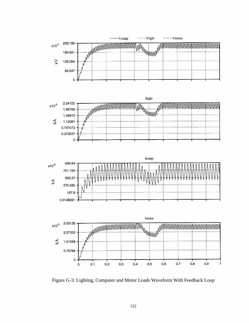
Figure G-3: Lighting, Computer and Motor Loads Waveform With Feedback Loop
122

123

124